Improving Recession Probability Forecasts in the U.S. Economy

Munechika Katayama∗

Louisiana State University

mkatayama@lsu.edu

This Draft: January 18, 2009

First Draft: July 2008

Abstract

There are two margins to improve forecasting models of the U.S. recession probability: in-

cluding additional variables and using different functional form. Using out-of-sample and cross

validation methods, I systematically compare the performance of various forecasting models that

differ in terms of variables included and functional forms used. I find substantial gains from

including additional variables, such as the S&P 500 and non-farm employment growth, together

with the term spread. In addition, there is a room to further improve forecasting accuracy by

utilizing a non-Normal cumulative distribution function. I also explore this possibility by using

the generalized Edgeworth expansion. Resulting predictions outperform ones from a typical

probit model in all three measures of forecasting accuracy considered.

∗I am indebted to James Hamilton for his encouragement and helpful comments. I have also benefited fromdiscussion with Hiroaki Kaido. This paper is based on Chapter 3 of my doctoral dissertation at UCSD.

1

1 Introduction

There are many attempts to forecast recessions in the U.S. economy. Information contained in

forward-looking variables can be used for making predictions about the future state of the econ-

omy. Stock and Watson (1989) report that the slope of the Treasury yield curve provides useful

information in constructing their leading indicator. Estrella and Mishkin (1998) examine the use-

fulness of financial variables in making predictions about future recession probabilities at various

forecasting horizons. They find that the slope of yield curve is the best single predictor of future

recession probabilities.1 Other studies also utilize the predictive content of the term spread in order

to forecast recession probabilities.2 Although developments in the literature achieve some success

in making predicting recession, there is a room to improve forecasting accuracy.

To obtain further improvements, there are two margins that we can exploit. One is the question

of selecting a set of predictor variables. The other is a choice of functional form. Typical studies on

forecasting recession probabilities utilize a simple binary response model, such as a probit or logit

model. In this paper, I will explore the importance of the two margins in improving forecasting

accuracy.

Within the class of probit/logit models, there is favorable evidence for benefits from including

additional information, other than the term spread. For example, Estrella and Mishkin (1998)

find some evidence on usefulness of including an additional variable, such as a New York Stock

Exchange index or GDP growth. Wright (2006) reports that including the level of the federal funds

rate together with the term spread results in better forecasting performance than the term spread

alone.3 King, Levin, and Perli (2007) recently find superior predictive power of the 5-year corporate

credit spread on AA-rated firms compared with the 10-year-3-month Treasury term spread over

the Great Moderation period (since the mid 1980’s). Furthermore, they also report that once

the corporate spread is augmented by the term spread, the forecasting performance dramatically

improves by reducing “false positive” predictions of recession.

There are also some attempts to extend a simple probit model in the recent literature. For ex-1Their finding is consistent with a simple rule of thumb that the Treasury yield curve inversions or negative

term spreads are likely followed by recessions in subsequent periods and the term spread has been cited as a leadingeconomic indicator.

2Other studies include Dotsey (1998), Birchenhall, Jessen, Osborn, and Simpson (1999), Estrella, Rodrigues, andSchich (2003), Stock and Watson (2003) and Clements and Galvao (2006).

3He also finds some evidence favorable for controlling for a term premium proxy.

2

ample, Chauvet and Potter (2005) extend a probit model in a way that it allows for business-cycle

dependent coefficients (i.e., multiple breaks) and/or autocorrelated errors. Kauppi and Saikkonen

(2008) develop dynamic probit models that include lagged explanatory variables and lagged reces-

sionary dummies. Dueker (2005) presents a framework (a Qual VAR) that enables us to treat a

qualitative variable as endogenous in a typical VAR framework, so that we can obtain dynamic

forecasts of the qualitative variable.

Going beyond the typical univariate probit model with the term spread, such as allowing ad-

ditional features in a forecasting model and/or including additional predictor variables most likely

would improve in-sample forecasting performance. However, at the same time, we also have to worry

about a potential over-fitting problem. Hansen (2008) examines the pitfalls of relying on in-sample

fit. He shows that too good in-sample fit (over-fitting) tends to be associated poor out-of-sample

fit and that model selection based on in-sample fit is not reliable. In addition, he demonstrates

that tendencies of yielding spurious results are much higher if we use in-sample evaluation and are

more pronounced when we compare performance of a large number of alternative models. In this

paper, therefore, I will use out-of-sample and cross validation methods to examine the importance

of the two margins that can contribute to improve forecasting performance.

First, I systematically compare the forecasting performance of 6-month-ahead recession prob-

ability predictions in the U.S. economy. I look at all possible combinations of 33 variables up to

trivariate models with 6 different functional forms. Results highlight the importance of variable

selection. Finding the best combination of predictor variables greatly improve forecasting perfor-

mance. Especially, among variables considered, the combination of the term spread, changes in the

S&P 500 stock price index, and growth rate of non-farm employment is found to achieve the best

forecasting accuracy. Furthermore, additional gains can be obtained by using non-Normal cumula-

tive distribution functions. However, there is some mixed evidence on what features of functional

form are necessary, in order to improve forecasting performance. Then, I proceed to allow for more

flexibility in the functional form by utilizing the generalized Edgeworth expansion of Jarrow and

Rudd (1982).

The rest of the paper is organized as follows. Section 2 presents basic binary response models

and associated results. Section 3 introduces the generalized Edgeworth expansion and applies it to

making predictions of the U.S. recession probability. Finally, Section 4 concludes.

3

2 Basic Models and Results

2.1 Recession Probability Forecasting Model

Let yt represent an NBER recession binary variable, which equals 1 when the economy is in recession

in month t and equals 0 in expansion. Typical models of forecasting h-period-ahead recession

probabilities using the information available at time t assume that

Prob(yt+h = 1|xt) = F (β′xt), (1)

where F (·) is a monotonically increasing function, whose range is the unit interval, β is a vector

of coefficients associated with a vector of predictors x′t = [1, x1,t, · · · , xk,t], and k is the number of

variables included.

It is commonly assumed that yt+h is a conditionally independent Bernoulli random variable, so

that the likelihood function is given by:

L =T∏t=1

[F (β′xt)

]yt+h [1− F (β′xt)]1−yt+h . (2)

In an empirical analysis, I will set h = 6 and focus on 6-month-ahead predictions.

In this formulation, predicting recession probability involves two issues that are possibly related

to each other. The first one is to choose a set of predictor variables, so that we can obtain useful

signals from data. A workhorse predictor in the literature is the Treasury term spread between

10-year and 3-month bonds, which is due to the finding in Estrella and Mishkin (1998).

Given a choice of F (·), finding a better combination of predictor variables obviously helps

improve forecasting accuracy if those variables contain different information and jointly provide

useful signals. Since there are no a priori variable selection procedures available, our approach

is to try all possible combinations of variables, in order to find a better combination of variables

that are useful in forecasting recession probabilities. Although knowing the best single predictor

is helpful, it is unlikely that we can obtain some insights about a better combination of variables

by just looking at forecasting performance of single predictors because those variables that show

relatively good forecasting performance tend to contain similar information.

4

The second issue is how to translate signals into a probability measure between 0 and 1, which

is related to a shape of F (·). In order to guarantee that F (·) is monotonically increasing and

takes values between 0 and 1, we typically use a known cumulative distribution function (CDF).

A popular choice is to use either the Standard Normal CDF (a probit model) or the Logistic CDF

(a logit model), or some variants of those (e.g., Chauvet and Potter, 2005; Kauppi and Saikkonen,

2008). However, the shape of F (·) is not necessarily restricted to typical ones. In principle, the

CDF of any continuous probability random variable will suffice.

Differences in the shape of CDFs can be characterized in terms of “skewness” and “excess

kurtosis”. It should be noted that it is not appropriate to use terms skewness and excess kurtosis

here because we are not talking about characteristics of underlying statistical distributions, but

just utilizing functional forms. However, for expositional simplicity, I will use those terms in

describing the shape of a CDF. The consequence of allowing skewness and excess kurtosis is as

follows. Higher excess kurtosis makes a CDF steeper around the median of β′x. On the other hand,

allowing non-zero skewness makes a CDF asymmetric around F (β′x) = 0.5. With zero skewness,

F (x) = 1− F (−x) for any x ∈ R. However, non-zero skewness implies F (x) 6= 1− F (−x).4

In order to understand what features of a CDF are helpful in improving forecasting accuracy,

I will consider 6 different CDFs. Table 1 summarizes characteristics of the CDFs considered.

In addition to the Standard Normal CDF and the Logistic CDF, I consider Student-t, Laplace,

Gumbel, and Type III Generalized Extreme Value (GEV3). All location parameters and scale

parameters, if applicable, are set to 0 and 1, respectively. These CDFs are chosen and configured

to incorporate non-zero skewness and/or higher excess kurtosis that the Standard Normal CDF

does not have. The first four CDFs have zero skewness and differ in terms of degree of excess

kurtosis. The Logistic CDF has excess kurtosis of 1.2. The degrees of freedom parameter for

Student-t is set to be 6.5, such that its excess kurtosis equals 2.4. The excess kurtosis of Laplace

is 3. The last two CDFs also have positive skewness. For the Gumbel CDF, skewness is equal to

1.1395 and excess kurtosis is 2.4. The shape parameter of the Type III GEV, s, is set such that its

excess kurtosis equals 3 (i.e., s = −0.1732). The associated skewness becomes 0.3492. Thus, for a

given set of predictor variables, I will be able to infer the importance of allowing for excess kurtosis4In general, changing location and scale parameters does not affect forecasting results and they are fixed to avoid

an identification problem. Changing the location parameter just changes the estimate of the constant term andchanging the variance just results in different scaling of coefficients β.

5

Table 1: List of the Cumulative Distribution Functions ConsideredType of CDF F (x) Skewness Excess Kurtosis

Standard Normal1√2π

∫ x

∞exp

(−u2

2

)du 0 0

Logisticexp(x)

1 + exp(x)0 1.2

Student-t with ν = 6.5∫ x

−∞

Γ(ν+12 )

√νπΓ(ν2 )

(1 +

u2

ν

)−(ν+1)2

du 0 2.4

Laplace12

[1 + sgn(x) {1− exp (−|x|)}] 0 3

Gumbel 1− exp {− exp(−x)} 1.1395 2.4

Type III GEV with s = −0.1732 exp{− (1 + sx)−1/s

}0.3492 3

Note: All location parameters are set to be 0 and all scale parameters are set to be 1. ν representsdegrees of freedom parameter for the Student-t distribution. Γ(·) is a gamma function. Excess kurtosis

of Student-t is given by 6/(ν − 4) for ν > 4. Skewness of the Gumbel distribution is 12√

6ζ(3)

π3 , whereζ(·) is a zeta function. s denotes a shape parameter of the generalized extreme value distribution. For

the Type III GEV, skewness is given by −Γ(1−3s)+3Γ(1−s)Γ(1−2s)−2(Γ(1−s))3

(Γ(1−2s)−(Γ(1−s))2)3/2 and excess kurtosis is give by

Γ(1−4s)−4Γ(1−s)Γ(1−3s)+6Γ(1−2s)(Γ(1−s))2−3(Γ(1−s))4

(Γ(1−2s)−(Γ(1−s))2)2 .

in F (·) by looking at results based on the first four CDFs. Furthermore, comparing the Gumbel

with the Student-t or the Type III GEV with the Laplace enables us to obtain some insight on

whether allowing positive skewness is helpful in improving forecasting performance.5

2.2 Data

Table 2 lists all 33 monthly variables considered in this paper. The sample period starts from April

1960, which corresponds to the beginning of the 1960-61 recession. It is chosen to maximize data

availability and include as many recession episodes as possible. Since it is often the case that a

decision of the NBER Business Cycle Dating Committee has a time lag,6 the sample period is ended

at the end of December, 2005. The data set contains the term spreads, the credit spreads, various5It is also possible to introduce negative skewness by using the Type III GEV. However, preliminary estimation

indicated that forecasting performance based on the Type III GEV with negative skewness is inferior to others ingeneral. So, I do not report their results.

6A substantial time lag of the announcement might be one disadvantage of using the NBER recessions to charac-terize the state of the economy. This motivates Chauvet and Hamilton (2006) to study algorithms that enable us toconstruct a real-time business cycle turning point.

6

interest rates, employment data, stock price indices, monetary aggregates, and other macroeco-

nomic variables. Most of those are investigated in the earlier studies or used in constructing a

composite leading indicator. It also includes variables, to which the NBER Business Cycle Dating

Committee pays particular attention in deciding business cycle peaks and troughs. Since Kane

(2008) documents the usefulness of employment data in predicting occurrence of recessions, the

data set includes employment-related variables as well.

Recently, King, Levin, and Perli (2007) report that, in the period of the Great Moderation,

the credit spread on AA-rated firms has particularly good forecasting performance. However, the

corporate bond yields used in their study (maturity of 5-year and 10-year) do not cover the entire

sample. Since there are not many recessionary periods, especially after the 1980’s, using shorter

sample periods may have considerable effects on evaluating forecasting performance. Thus, I have

decided not to include the credit spreads that King, Levin, and Perli (2007) have used. Instead, as

a crude proxy, the data set include spreads between Moody’s AAA-, AA-, or A- rated corporate

bond yield (20 years or longer) and the 10-year Treasury bond yield.7

When we focus on financial variables as predictors, we do not need to consider a gap between

when an observation is made and when it is available for forecasting. However, as shown in Table

2, some series are not reported immediately and we need to take account of the information lag,

in order to accurately assess forecasting models. In this paper, any variable zt represents the

latest data on z available at month t, instead of an observation at month t. For example, industrial

production (IP) has 1 month of the information lag. So, IP2000:01 refers to the industrial production

data on December 1999.

Because the total number of models increases exponentially as the number of variables included

(k) increases, I will restrict my attention to k ≤ 3. This will result in examining a total of∑3k=1

33!k!(33−k!) × 6 = 36102 forecasting models.

7Since the 20-year Treasury bond yield data has discontinuity between January 1987 and September 1993, I usethe 10-year T-bond rate, instead. Thus, precisely speaking, this “credit spread” is a combination of the “true” creditspread and the term spread.

7

Table 2: List of VariablesPredictor Description Info.

LagInterest Rates 0

FF Federal Funds rate 03M 3-month Treasury Bill rate 05Y 5-year Treasury Bond rate 010Y 10-year Treasury Bond rate 0AAA Moody’s corporate bond yield, AAA 20 years or longer 0AA Moody’s corporate bond yield, AA 20 years or longer 0A Moody’s corporate bond yield, A 20 years or longer 0

Term SpreadsTS10YFF 10Y-FF Treasury term spread 0TS10Y3M 10Y-3M Treasury term spread 0TS10Y5Y 10Y-5Y Treasury term spread 0

Credit SpreadsCSAAA AAA - 10Y spread 0CSAA AA - 10Y spread 0CSA A - 10Y spread 0

Employment DataEMP Non-agricultural employment (log-differenced) 0CEMP Civilian employment (log-differenced) 0UICLAIM Initial unemployment insurance claims (log-differenced) 1UNEMP Unemployment rate 0UNEMPD Changes in unemployment rate 0HOURS Average weekly hours in manufacturing (log-differenced) 0

Stock Price IndicesDJ30 Dow Jones 30 average (% changes over 3 months) 0SP500 S&P 500 stock price index (% changes over 3 months) 0

Monetary AggregatesM0 Monetary base (log-differenced) 1M1 M1 (log-differenced) 1M2 M2 (log-differenced) 2

Other Macroeconomic VariablesCLI11 Composite leading indicators (11 series, 1987=100, log-differenced) 1CPI CPI, all urban, all items (log-differenced) 1EXP Consumer expectation (1966.1 = 100) 0EXPD Changes in consumer expectation 0HOUSE New private housing units authorized by building permits (log-differenced) 1VENDOR Vendor performance (slower deliveries diffusion index, %) 0INCOME Personal income less transfer payments (log-differenced) 2IP Industrial production (log-differenced) 1SALES Manufacturing & trade sales (log-differenced) 1

Note: Information lag is measured at the end of month. Strictly speaking, those employment data with zeroinformation lag and vendor performance are not available at the end of the month. However, they will beavailable at the very beginning of the next month and there are virtually no considerable lags. Thus, theyare categorized in the zero information lag variable.

8

2.3 Evaluating Forecasting Performance

In order to evaluate various forecasting models, I will primarily focus on out-of-sample results.

Hansen (2008) shows that in-sample and out-of-sample fits are negatively correlated, which implies

that good in-sample performance is not a useful indicator of out-of-sample accuracy and that relying

on in-sample fit is highly misleading. This over-fitting problem is particularly important, since the

likelihood of obtaining spurious results is more pronounced when we search a large number of

alternative models. For this reason, I will focus on recursive out-of-sample forecasting evaluation

and I will use cross validation as a robustness check.

For recursive (pseudo) out-of-sample forecasting exercises, the out-of-sample prediction starts

from January 1989 and ends at the end of the full sample. The out-of-sample period covers the last

two recessions in the U.S. economy. By adding observations one by one, I estimate a forecasting

model again to produce a forecast for the next month. In reality, when we forecast future recession

probability, we are not certain about the true state of the economy in recent months. It is because

the decision of the NBER Business Cycle Dating Committee typically involves substantial time lag.

To be realistic, I assume that forecasters do not know the true state of the economy for a year and

assume that yt = · · · = yt−11 = yt−12, that is, the economy is in the same state as a year ago.

Following Clements and Galvao (2006), I will use three different measures for evaluating ac-

curacy of out-of-sample recession probability predictions. The first measure is the probability-

analogue of mean squared error, the quadratic probability score (QPS), which is commonly used

in evaluating probability forecasts. The QPS is defined as

QPS =2T

T∑t=1

(pt − yt)2, (3)

where pt is the recession probability forecast month t. The QPS takes values between 0 and 2 and

smaller value indicates more accurate forecasts.

The second measure is the log probability score (LPS), which is defined as

LPS = − 1T

T∑t=1

{yt log(pt) + (1− yt) log(1− pt)

}. (4)

The LPS ranges from 0 to +∞ and a smaller value corresponds to more accurate predictions and

9

penalizes larger mistakes more heavily than the QPS.

The last measure is the Kuipers Score (KS), which is given by

KS =

∑Tt=1 yt1(pt>0.5)∑T

t=1 yt−∑T

t=1(1− yt)1(pt>0.5)∑Tt=1(1− yt)

, (5)

= hit rate− false rate,

where 1(·) is an indicator function that equals 1 if its argument is true and 0 otherwise. The KS

calculates the difference between the hit rate and the rate of false signals by using 50% probability

of recession as a cutoff. The KS takes values between −1 and 1. A score of 1 corresponds to

making perfect predictions. The KS evaluates the recession predictions from a slightly different

aspect, compared with other two measures. Even when recession predictions never show “strong”

indications (say, higher than 50% probability), it is possible to have seemingly good results based

on the QPS and LPS. The KS discounts such “weak” predictions. In this sense, the KS captures

the strength and accuracy of predictions by using the 50% probability cutoff.

There is a potential problem of just relying on the recursive out-of-sample exercises described

above, especially in the context of recession probability forecasting. Since there are not many reces-

sions in the out-of-sample period, it is possible to select a forecasting model that has particularly

good performance for the last two recessions, but not for other recessions or a next recession.

In order to robustify the results, I will also carry out a cross-validation type exercise, called

leaving 2-years out. The detailed procedures of the leaving 2-years out exercises are as follows. Let

S = {(yt,xt−h) : t = 1, · · · , T} denote a full sample and Lτ = {(yt,xt−h) : t = τ − 12, · · · , τ + 12}

represent a set of excluding observations. For each τ = 13, · · · , T − 12,

(i) Take Eτ = S \ Lτ as a training sample.

(ii) Estimate parameter values βτ based on Eτ .

(iii) Make a prediction for yτ by using βτ and xτ−h and store it.

(iv) Repeat steps (i) – (iii).

Then calculate QPS, LPS, and KS based on {yτ}T−12τ=13 .

10

2.4 Results

2.4.1 Univariate Probit Models

First, we will start off by looking at forecasting performance within a class of univariate probit

models of predicting 6-month-ahead recession probabilities (h = 6) as a benchmark. Table 3

summarizes the out-of-sample forecasting performance of univariate probit models.

The rankings of out-of-sample forecasting accuracy based on the QPS and the LPS have similar

patterns, with a few exceptions. The term spread between 10-year and 3-month Treasury bonds

(TS10Y3M), which is commonly used, and the term spread between 10-year bond and the Federal

Funds rate (TS10YFF) are the best predictors based on the QPS and LPS, respectively. However,

the term spread between 10-year and 5-year bonds (TS10Y5Y) has poorer out-of-sample perfor-

mance in the both measures. In contrast to the term spread, the credit spreads (CSA, CSAA, and

CSAAA) have poor forecasting performance. Among other variables, the levels of interest rates (FF

and 3M) and the composite leading indicators (CLI11) might be useful predictors as well. However,

employment related variables, those variables that the NBER Business Cycle Dating Committee is

paying attention to, and monetary aggregates have considerably poorer results.

It is interesting to point out that, in terms of quadratic loss, the conventional term spread

(TS10Y3M) outperforms the one based on the Federal Funds rate. However, if we penalize larger

mistakes more heavily, then the out-of-sample forecasting performance improves by using TS10YFF.

That is, TS10Y3M minimizes the quadratic loss, but it results some larger mistakes. The same

thing is true for the levels of FF and 3M.

The out-of-sample forecasting performance evaluated by using the KS gives us a completely

different picture. Most predictor variables have non-positive values for the KS. In other words,

they usually do not give us strong predictions about the occurrence of future recessions or correct

predictions are largely offset by false predictions. In the worst case, we will get more false signals,

which indicate more than 50% probability of a recession during an expansion, than correct ones.

The only variable that has a positive value for the KS is the growth rate of M2. However, other

measures of forecasting performance suggest that the performance of M2 is one of the poorest,

among predictor variables considered. The opposite can also happen. Although CLI11 has relatively

11

Table 3: Variable Rankings with Univariate Probit ModelsQPS Ranking LPS Ranking KS Ranking

TS10Y3M 0.1399 TS10YFF 0.2396 M2 0.0179TS10YFF 0.1444 TS10Y3M 0.2401 TS10YFF 0.00003M 0.1488 FF 0.2607 TS10Y3M 0.0000FF 0.1503 3M 0.2637 FF 0.0000CLI11 0.1541 CLI11 0.2733 3M 0.0000CPI 0.1579 SP500 0.2877 CPI 0.00005Y 0.1610 CPI 0.2964 5Y 0.0000SP500 0.1627 5Y 0.2993 10Y 0.000010Y 0.1650 10Y 0.3081 A 0.0000A 0.1663 A 0.3094 AAA 0.0000AAA 0.1665 AAA 0.3098 AA 0.0000AA 0.1669 AA 0.3108 UICLAIM 0.0000UICLAIM 0.1695 UICLAIM 0.3131 EXPD 0.0000CSAAA 0.1712 DJ30 0.3146 IP 0.0000TS10Y5Y 0.1725 EXPD 0.3216 UNEMPD 0.0000EXPD 0.1733 IP 0.3227 SALES 0.0000IP 0.1736 UNEMPD 0.3237 UNEMP 0.0000CSAA 0.1740 TS10Y5Y 0.3241 EMP 0.0000UNEMPD 0.1742 SALES 0.3277 HOURS 0.0000UNEMP 0.1759 UNEMP 0.3284 M0 0.0000HOURS 0.1765 EMP 0.3284 CEMP 0.0000M0 0.1767 HOURS 0.3292 HOUSE 0.0000DJ30 0.1768 M0 0.3302 VENDOR 0.0000CEMP 0.1769 CEMP 0.3303 M1 0.0000SALES 0.1775 HOUSE 0.3325 CSA 0.0000EMP 0.1778 VENDOR 0.3349 CSAA 0.0000HOUSE 0.1782 EXP 0.3362 CSAAA 0.0000VENDOR 0.1791 INCOME 0.3480 CLI11 -0.0054CSA 0.1808 M1 0.3494 EXP -0.0054EXP 0.1854 CSA 0.3511 INCOME -0.0108INCOME 0.1923 CSAA 0.3694 DJ30 -0.0161M1 0.1927 M2 0.4214 TS10Y5Y -0.0215M2 0.2498 CSAAA 0.4261 SP500 -0.0323

12

1965 1970 1975 1980 1985 1990 1995 2000 2005

0.2

0.4

0.6

0.8

1TS10Y3MTS10YFF

(a) In-Sample Fit

1990 1991 1992 1993 1994 1995 1996 1997 1998 1999 2000 2001 2002 2003 2004 20050

0.2

0.4

0.6

0.8

1TS10Y3MTS10YFF

(b) Out-of-Sample Prediction

Figure 1: Predictions with Univariate Probit ModelsNote: The shaded areas represent the NBER recessions. Horizontal axes measures recession probabilities.

good performance based on other measures, it has a negative value for the KS.

Figure 1 presents in-sample (i.e., the entire sample) and out-of-sample 6-month-ahead predic-

tions from univariate probit models with TS10YFF and TS10Y3M. The shaded areas indicate the

recession periods. The top panel shows in-sample fit. As can be seen, the term spreads well capture

recessions and expansions in early periods, especially those in the 1970’s and 1980’s. However, it

seems that they do not provide strong predictions for the last two recessions.8 Particularly, for the

1990-91 recession, the predictions made by the term spreads miss the timing of the recession and8In conjunction with the Great Moderation, some researchers find instability of the predictive power of the term

spread (for example, Chauvet and Potter, 2005). However, Estrella, Rodrigues, and Schich (2003) do not find evidenceof a structural break in the binary response model.

13

Table 4: Top 20 Univariate Models

QPS Ranking LPS Ranking KS RankingCDF x1 QPS CDF x1 LPS CDF x1 KS

Laplace TS10Y3M 0.1360 Gumbel TS10YFF 0.2362 Laplace TS10Y3M 0.1111Student-t TS10Y3M 0.1388 GEV3 TS10YFF 0.2370 Laplace CLI11 0.0448Logistic TS10Y3M 0.1388 Laplace TS10Y3M 0.2392 Laplace SP500 0.0233Normal TS10Y3M 0.1399 Normal TS10YFF 0.2396 GEV3 SP500 0.0233GEV3 TS10Y3M 0.1410 Normal TS10Y3M 0.2401 Gumbel SP500 0.0233Gumbel TS10Y3M 0.1421 GEV3 TS10Y3M 0.2401 Normal M2 0.0179Normal TS10YFF 0.1444 Logistic TS10Y3M 0.2406 Gumbel TS10YFF 0.0000GEV3 TS10YFF 0.1446 Gumbel TS10Y3M 0.2408 GEV3 TS10YFF 0.0000Logistic TS10YFF 0.1453 Student-t TS10Y3M 0.2410 Normal TS10YFF 0.0000Student-t TS10YFF 0.1455 Logistic TS10YFF 0.2430 Normal TS10Y3M 0.0000Gumbel TS10YFF 0.1459 Student-t TS10YFF 0.2436 GEV3 TS10Y3M 0.0000Laplace TS10YFF 0.1459 Laplace TS10YFF 0.2463 Logistic TS10Y3M 0.0000Gumbel 3M 0.1482 Gumbel FF 0.2564 Gumbel TS10Y3M 0.0000GEV3 3M 0.1484 GEV3 FF 0.2582 Student-t TS10Y3M 0.0000Normal 3M 0.1488 Normal FF 0.2607 Logistic TS10YFF 0.0000Gumbel FF 0.1491 Gumbel 3M 0.2615 Student-t TS10YFF 0.0000Logistic 3M 0.1494 GEV3 3M 0.2623 Laplace TS10YFF 0.0000Student-t 3M 0.1495 Normal 3M 0.2637 Gumbel FF 0.0000GEV3 FF 0.1496 Logistic FF 0.2640 GEV3 FF 0.0000Normal FF 0.1503 Student-t FF 0.2644 Normal FF 0.0000

they do not have strong signals. This difficulty is also noted in other studies.9

The same is true for the out-of-sample forecasts, which are shown at the bottom panel of Figure

1. Although both the QPS and LPS select TS10YFF and TS10Y3M as the first two univariate

probit models, actual predictions are relatively poor and never exceed 50%. Furthermore, as in

the in-sample case, out-of-sample predictions also miss the timing of the 1990-91 recession. This

illustrates importance of paying attention to the KS, according to which both models score zero.

2.4.2 Univariate Models

Now we will look at the performance of univariate models based on alternative CDFs, which allow

positive skewness and/or excess kurtosis. Table 4 summarizes the ranking of univariate models

based on out-of-sample fit.

In terms of the QPS, as in the probit model, models with TS10Y3M provide better out-of-

sample forecasting accuracy than those with TS10YFF. For TS10Y3M, there is a clear indication9See Stock and Watson (2003) for a more detailed discussion.

14

of a better prediction for CDFs with excess kurtosis and the Laplace CDF achieves the best QPS.

On the other hand, allowing for skewness deteriorates forecasting accuracy, such as GEV3 and

Gumbel. However, such a pattern does not hold for TS10YFF and, in fact, the Normal CDF

outperforms other CDFs among univariate models with TS10YFF.

If we penalize larger mistakes more heavily than the QPS, the variable ranking based on the

LPS suggests some roles played by allowing skewness and excess kurtosis. For TS10YFF, allowing

positive skewness and excess kurtosis contributes to reducing large mistakes, compared with the

Normal. However, just incorporating excess kurtosis, but not skewness, appears to perform worse

than the Normal CDF and also than univariate models with TS10Y3M. Although, within the

probit models, TS10Y3M is inferior to TS10YFF, using the Laplace CDF improves the LPS and

achieves a better result than TS10YFF with the Normal. It is possible to obtain better forecasting

performance by employing non-Normal CDFs. However, it is not clear what additional features of

the functional form are helpful and it seems to be variable specific.

The rankings based on the QPS and LPS suggest that information contained in 3M helps reduce

quadratic loss, whereas information contained in FF tends to reduce larger mistakes.

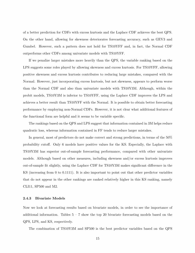
In general, most of predictors do not make correct and strong predictions, in terms of the 50%

probability cutoff. Only 6 models have positive values for the KS. Especially, the Laplace with

TS10Y3M has superior out-of-sample forecasting performance, compared with other univariate

models. Although based on other measures, including skewness and/or excess kurtosis improves

out-of-sample fit slightly, using the Laplace CDF for TS10Y3M makes significant difference in the

KS (increasing from 0 to 0.1111). It is also important to point out that other predictor variables

that do not appear in the other rankings are ranked relatively higher in this KS ranking, namely

CLI11, SP500 and M2.

2.4.3 Bivariate Models

Now we look at forecasting results based on bivariate models, in order to see the importance of

additional information. Tables 5 – 7 show the top 20 bivariate forecasting models based on the

QPS, LPS, and KS, respectively.

The combination of TS10Y3M and SP500 is the best predictor variables based on the QPS

15

Table 5: Top 20 Bivariate Models by the QPSCDF x1 x2 QPS

Laplace TS10Y3M SP500 0.1144Student-t TS10Y3M SP500 0.1144Logistic TS10Y3M SP500 0.1144Normal TS10Y3M SP500 0.1151GEV3 TS10Y3M SP500 0.1160Gumbel TS10Y3M SP500 0.1173GEV3 TS10YFF SP500 0.1226Student-t TS10YFF SP500 0.1228Logistic TS10YFF SP500 0.1228Gumbel TS10YFF SP500 0.1230Normal TS10YFF SP500 0.1230Laplace TS10YFF SP500 0.1236Laplace TS10Y3M EMP 0.1254Logistic TS10Y3M EMP 0.1268Student-t TS10Y3M EMP 0.1268Normal TS10Y3M EMP 0.1277GEV3 TS10Y3M EMP 0.1283Gumbel 3M SP500 0.1290Gumbel TS10Y3M EMP 0.1295Gumbel FF SP500 0.1298

Table 6: Top 20 Bivariate Models by the LPSCDF x1 x2 LPS

GEV3 TS10Y3M SP500 0.1984Normal TS10Y3M SP500 0.1985Gumbel TS10Y3M SP500 0.1993Logistic TS10Y3M SP500 0.1994Student-t TS10Y3M SP500 0.1997Laplace TS10Y3M SP500 0.2020Gumbel TS10YFF SP500 0.2027GEV3 TS10YFF SP500 0.2037Normal TS10YFF SP500 0.2064Logistic TS10YFF SP500 0.2084Student-t TS10YFF SP500 0.2087Laplace TS10YFF SP500 0.2112Gumbel FF SP500 0.2113Gumbel 3M SP500 0.2129GEV3 FF SP500 0.2146GEV3 3M SP500 0.2149GEV3 TS10Y3M EMP 0.2152Gumbel TS10Y3M EMP 0.2154Normal TS10Y3M EMP 0.2166Logistic TS10Y3M EMP 0.2172

and LPS. All three measures of out-of-sample accuracy suggest that it is important to include a

measure of term spread (either TS10Y3M or TS10YFF). Interestingly, there are some variables that

have relatively poor performance in univariate models and produce good out-of-sample forecasting

accuracy, together with the term spread measure. According to the rankings based on the univariate

models, SP500 and EMP are not a useful single predictor. Especially, EMP has relatively poor

out-of-sample forecasting performance. However, they become an important companion variable

to the term spread. In fact, those variables with the term spread are better than a combination of

two term spreads (TS10Y3M and TS10YFF), which are in the best two variables among univariate

models. This suggests that those variables contain some useful information that the term spread

does not have and also indicates that the univariate ranking is not a helpful guide for choosing

multiple predictors.

The importance of SP500 together with TS10Y3M is consistent with the finding of Estrella and

Mishkin (1998). In our bivariate models, even without being combined with the term spread, some

bivariate models that contain SP500 perform relatively well. However, it should be mentioned that

King, Levin, and Perli (2007) do not find superiority of SP500 in conjunction with the term spread.

Rather, they report that a combination of variables, which have better performance in univariate

16

Table 7: Top 20 Bivariate Models by the KSCDF x1 x2 KS

Laplace TS10Y3M EMP 0.2724GEV3 TS10Y3M SP500 0.2115Normal TS10Y3M SP500 0.2115Gumbel TS10Y3M SP500 0.2115Logistic TS10Y3M SP500 0.2115Student-t TS10Y3M SP500 0.2115Laplace TS10Y3M SP500 0.2115Laplace UICLAIM SP500 0.1900Laplace TS10Y3M EXPD 0.1667Laplace TS10Y3M VENDOR 0.1667Laplace TS10Y3M CSA 0.1613Laplace TS10Y3M M1 0.1559Gumbel UICLAIM SP500 0.1344GEV3 UICLAIM SP500 0.1344Normal UICLAIM SP500 0.1344Student-t UICLAIM SP500 0.1344Logistic UICLAIM SP500 0.1344Laplace TS10Y3M M2 0.1344Gumbel EMP SP500 0.1290Laplace IP SP500 0.1290

models, also perform better in bivariate models.10

Unlike the univariate models, combining SP500 with TS10Y3M always achieves the better per-

formance both in terms of the QPS and LPS than those models with TS10YFF. For the combination

of TS10Y3M and SP500, allowing only excess kurtosis helps improve the QPS, while including both

skewness and excess kurtosis contributes to improving the LPS and KS. Allowing both skewness

and excess kurtosis, in general, improves the LPS by reducing large false predictions. However,

there is some mixed evidence for the QPS in terms of the role of skewness and excess kurtosis. At

least, for the models with TS10Y3M, it seems better to allow only excess kurtosis, but not positive

skewness.

Although forecasting performance generally improves by adding one more predictor, probably

the biggest gain appears in the KS. In univariate models, only 6 models out of 198 have positive

scores. In bivariate models, 348 models out of 3168 have at least positive values for the KS.

Furthermore, the best model (TS10Y3M and EMP with the Laplace) scores more than twice as10This could be because of a couple of reasons. First, it could be attributed to the difference in periods used for

the out-of-sample forecasting exercises and forecasting horizon. Second, it might be because of the fact that my dataset does not include the credit spread measures that they use and perform quite well in their univariate models.Finally, it could be due to the difference in evaluating out-of-sample forecasting performance. They look at averageout-of-sample predictions over two test periods, the 2001 recession and the post-2001 expansion.

17

Table 8: Top 20 Models by the QPS

CDF x1 x2 x3 QPSLaplace TS10Y3M SP500 EMP 0.1051Logistic TS10Y3M SP500 EMP 0.1074Student-t TS10Y3M SP500 EMP 0.1074Student-t TS10Y3M SP500 A 0.1079Laplace TS10Y3M SP500 A 0.1080Logistic TS10Y3M SP500 A 0.1081Student-t TS10Y3M SP500 AAA 0.1084Logistic TS10Y3M SP500 AAA 0.1086Student-t TS10Y3M SP500 AA 0.1087Logistic TS10Y3M SP500 AA 0.1088Laplace TS10Y3M SP500 AAA 0.1088Normal TS10Y3M SP500 EMP 0.1089Laplace TS10Y3M SP500 AA 0.1090GEV3 TS10Y3M SP500 A 0.1092Normal TS10Y3M SP500 A 0.1093Laplace TS10Y3M SP500 IP 0.1093GEV3 TS10Y3M SP500 AAA 0.1098Normal TS10Y3M SP500 AAA 0.1098GEV3 TS10Y3M SP500 AA 0.1100GEV3 TS10Y3M SP500 EMP 0.1100

Table 9: Top 20 Models by the LPS

CDF x1 x2 x3 LPSGEV3 TS10Y3M SP500 A 0.1832Gumbel TS10Y3M SP500 A 0.1834GEV3 TS10Y3M SP500 AAA 0.1843GEV3 TS10Y3M SP500 AA 0.1845Gumbel TS10Y3M SP500 AAA 0.1847Gumbel TS10Y3M SP500 AA 0.1848Gumbel 5Y SP500 3M 0.1848Student-t TS10Y3M SP500 A 0.1852Logistic TS10Y3M SP500 A 0.1852Normal TS10Y3M SP500 A 0.1853GEV3 TS10Y3M SP500 EMP 0.1857GEV3 5Y SP500 3M 0.1857Gumbel TS10Y3M SP500 10Y 0.1858Gumbel TS10Y3M SP500 3M 0.1858Gumbel 10Y SP500 3M 0.1858Gumbel TS10Y3M SP500 EMP 0.1859Student-t TS10Y3M SP500 AAA 0.1861Logistic TS10Y3M SP500 AAA 0.1861Normal TS10Y3M SP500 AAA 0.1861GEV3 TS10Y3M SP500 10Y 0.1862

high as the best univariate model.

2.4.4 Trivariate Models and Overall Rankings

Now we turn our attention to the overall forecasting performance, including all of univariate,

bivariate, and trivariate models with 6 different CDFs. Tables 8 – 10 list the top 20 forecasting

models out of 36102 forecasting models, based on different criteria.

The Laplace with TS10Y3M, SP500, and EMP is the best forecasting model based on the QPS

and KS. Regardless of the functional form used, this variable combination records relatively good

out-of-sample performance. This is consistent with the bivariate results that SP500 and EMP

perform relatively better in conjunction with the term spread measure.

However, the combination of TS10Y3M, SP500, and EMP tend to make larger prediction errors,

compared to the combination that includes corporate bond yields on A-rated firms (A), instead

of EMP. The combination of TS10Y3M, SP500, and A is the best in terms of the LPS. It is also

the second best in the QPS ranking. However, this variable combination does not result in good

18

Table 10: Top 20 Models by the KSCDF x1 x2 x3 KS

Laplace TS10Y3M SP500 EMP 0.3835Normal TS10Y3M SP500 EMP 0.3333Logistic TS10Y3M SP500 EMP 0.3280Student-t TS10Y3M SP500 EMP 0.3280Logistic TS10Y3M SP500 IP 0.3280Student-t TS10Y3M SP500 IP 0.3280Laplace TS10Y3M SP500 IP 0.3280GEV3 TS10Y3M SP500 EMP 0.3172Laplace UNEMP SP500 A 0.3172Laplace UNEMP SP500 AA 0.3172Gumbel TS10Y3M SP500 EMP 0.3118GEV3 TS10Y3M M2 CSA 0.2957Gumbel TS10Y3M M2 CSA 0.2957Laplace TS10Y3M EMP 0.2724GEV3 TS10Y3M SP500 UNEMPD 0.2724Normal TS10Y3M SP500 UNEMPD 0.2724Logistic TS10Y3M SP500 UNEMPD 0.2724Gumbel TS10Y3M SP500 UNEMPD 0.2724Student-t TS10Y3M SP500 UNEMPD 0.2724Laplace TS10Y3M SP500 UNEMPD 0.2724

performance in terms of the KS.

It is worthwhile to point out the importance of TS10Y3M and SP500, regardless of the fore-

casting accuracy measures. Thus, improving out-of-sample forecasting accuracy could be a task of

choosing a good companion variable to this combination. In this sense, other corporate bond yields

(AA and AAA) are also good companion variables. Although in the bivariate models, the term

spread measure TS10YFF was one of the best predictors together with SP500, augmenting the

combination of TS10Y3M and SP500 with other variables outperforms the TS10YFF counterparts.

Except for the combination of TS10Y3M, SP500, and EMP, the variable combinations that are

ranked relatively high in the KS ranking do not have good out-of-sample forecasting performance

in terms of the QPS or LPS. In other words, making strong predictions during recessions involves

risks of making positive false signals during expansions, which worsens the QPS and LPS. In out-

of-sample forecasting exercises, there is some favorable evidence for allowing excess kurtosis to

improve the QPS and KS, whereas adding positive skewness could improve forecasting accuracy in

terms of the LPS.

19

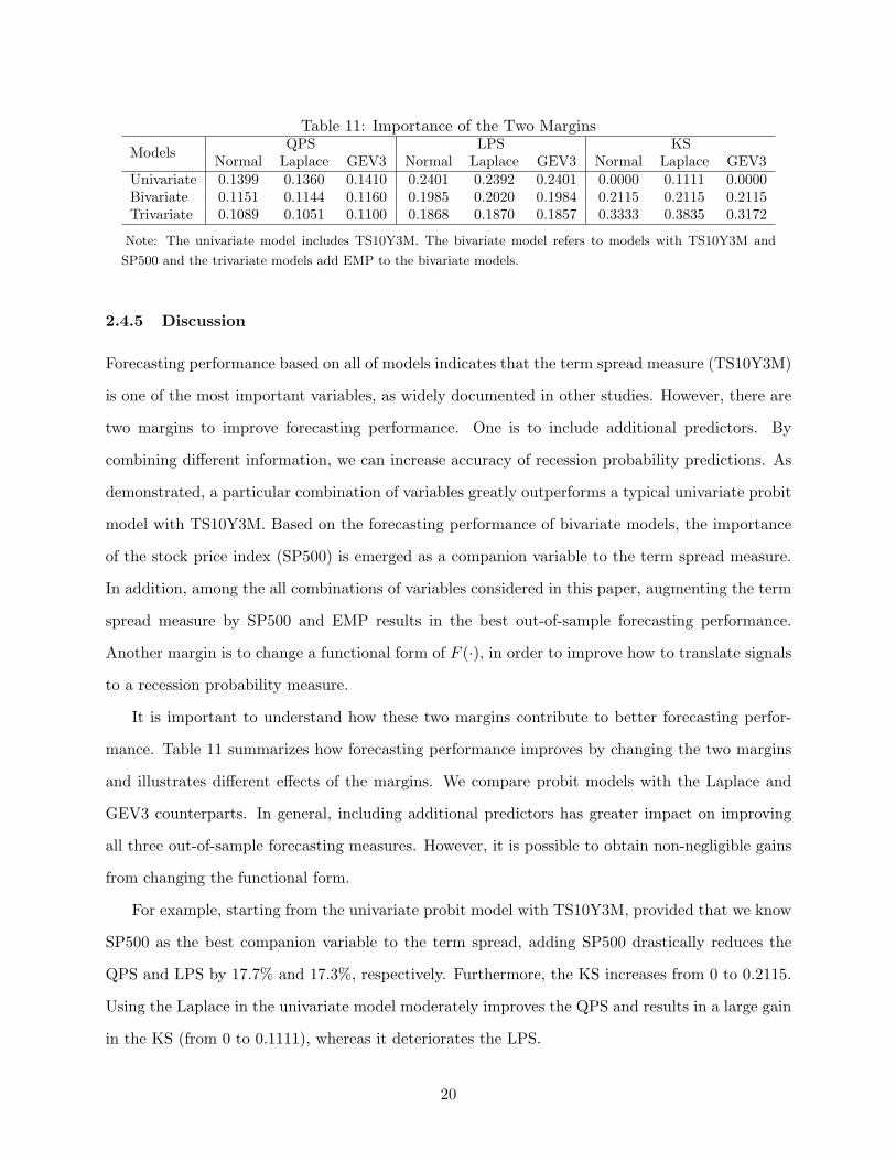
Table 11: Importance of the Two Margins

Models QPS LPS KSNormal Laplace GEV3 Normal Laplace GEV3 Normal Laplace GEV3

Univariate 0.1399 0.1360 0.1410 0.2401 0.2392 0.2401 0.0000 0.1111 0.0000Bivariate 0.1151 0.1144 0.1160 0.1985 0.2020 0.1984 0.2115 0.2115 0.2115Trivariate 0.1089 0.1051 0.1100 0.1868 0.1870 0.1857 0.3333 0.3835 0.3172

Note: The univariate model includes TS10Y3M. The bivariate model refers to models with TS10Y3M and

SP500 and the trivariate models add EMP to the bivariate models.

2.4.5 Discussion

Forecasting performance based on all of models indicates that the term spread measure (TS10Y3M)

is one of the most important variables, as widely documented in other studies. However, there are

two margins to improve forecasting performance. One is to include additional predictors. By

combining different information, we can increase accuracy of recession probability predictions. As

demonstrated, a particular combination of variables greatly outperforms a typical univariate probit

model with TS10Y3M. Based on the forecasting performance of bivariate models, the importance

of the stock price index (SP500) is emerged as a companion variable to the term spread measure.

In addition, among the all combinations of variables considered in this paper, augmenting the term

spread measure by SP500 and EMP results in the best out-of-sample forecasting performance.

Another margin is to change a functional form of F (·), in order to improve how to translate signals

to a recession probability measure.

It is important to understand how these two margins contribute to better forecasting perfor-

mance. Table 11 summarizes how forecasting performance improves by changing the two margins

and illustrates different effects of the margins. We compare probit models with the Laplace and

GEV3 counterparts. In general, including additional predictors has greater impact on improving

all three out-of-sample forecasting measures. However, it is possible to obtain non-negligible gains

from changing the functional form.

For example, starting from the univariate probit model with TS10Y3M, provided that we know

SP500 as the best companion variable to the term spread, adding SP500 drastically reduces the

QPS and LPS by 17.7% and 17.3%, respectively. Furthermore, the KS increases from 0 to 0.2115.

Using the Laplace in the univariate model moderately improves the QPS and results in a large gain

in the KS (from 0 to 0.1111), whereas it deteriorates the LPS.

20

Univariate vs. Trivariate

1990 1991 1992 1993 1994 1995 1996 1997 1998 1999 2000 2001 2002 2003 2004 20050

0.2

0.4

0.6

0.8

1Univariate ProbitTrivariate Probit

Difference between Laplace and Probit

1990 1991 1992 1993 1994 1995 1996 1997 1998 1999 2000 2001 2002 2003 2004 2005−0.1

0

0.1

Difference between GEV3 and Probit

1990 1991 1992 1993 1994 1995 1996 1997 1998 1999 2000 2001 2002 2003 2004 2005−0.02

0

0.02

0.04

Figure 2: Comparison of Out-of-Sample Predictions

Note: Shaded areas indicate the NBER recession episodes. The top panel compares predictions from the univariate

probit model with TS10Y3M with those from the trivariate models with TS10Y3M, SP500, and EMP. The middle and

bottom panels show differences in predictions by changing the functional form. The middle panel plots the difference

between the trivariate Laplace and the trivariate probit and the bottom panel depicts the difference between the

trivariate GEV3 and the trivariate probit.

Although marginal gains become smaller, adding the third variable (EMP) further improves the

out-of-sample forecasting performance of the probit model. Using the Laplace improves the QPS

and KS of the trivariate model. While only allowing for the excess kurtosis (Laplace) cannot improve

the LPS, allowing both skewness and excess kurtosis (GEV3) can improve the LPS, compared with

the probit model, however. In sum, the QPS and KS can be improved by using the Laplace, whereas

using the GEV3 can improve the LPS.

The top panel of Figure 2 compares out-of-sample predictions from the univariate probit model

with the term spread with the trivariate probit model (TS10Y3M, SP500, and EMP). As can

be seen, including additional variables reduces forecasting errors during expansions. Especially,

21

predictions from the univariate model suggest moderate possibilities of recessions during the last

half of the 1990’s, when the economy was in fact in the longest expansion. Those positive predictions

are dampened by including additional variables. At the same time, it contributes to making stronger

predictions during recessions, especially for the last recession. However, in exchange for such

improvements, the trivariate model also contains a couple of relatively strong false positive signals

during expansions, which are not present in the univariate model.

The middle panel of Figure 2 plots differences in predictions between the trivariate Laplace

model and the trivariate probit model. This suggests some benefits from changing functional form.

Using the Laplace, instead of the Normal, will amplify positive signals during the 2001 recession

and also will dampen strong false positive signals that happen right after the 1990-91 recession and

before and after the 2001 recession. In general, using the Laplace will contribute to amplifying

strong signals and to dampening weak signals, so that on average there will be less forecasting

errors. However, such a feature works in an unfavorable way during the 1990-91 recession, since

the underlying predictions are somewhat weak and miss the correct timing.

The bottom panel of Figure 2 plots differences in predictions between the trivariate GEV3

model and the trivariate probit model. Overall, differences between the GEV3 model and the

probit model are somewhat small. Unlike the Laplace model, using the GEV3 improves predictions

for the 1990-91 recession. However, early periods of the 2001 recession have weaker predictions

than the probit model. Although using the GEV3 will reduce false positive predictions during

expansions, strong false positive signals are, in fact, amplified.

Although there are some trade-offs in using different functional forms, as indicated in Table 11,

additional features in a forecasting model can improve out-of-sample forecasts.

2.4.6 Robustness Check

As a robustness check, I also evaluate forecasting performance of all models using the leaving 2-years

out exercises. Differences in the results that the leaving 2-years out typically selects TS10YFF as

a measure of a term spread, instead of TS10Y3M. Figure 3 compares forecasting performance of

models including TS10Y3M and TS10YFF in the both exercises.

In general, those models that include TS10Y3M work relatively better in the out-of-sample

22

0.1 0.11 0.12 0.13 0.14 0.15 0.16 0.17 0.18 0.190.1

0.12

0.14

0.16

0.18

0.2

0.22

0.24

QPS (Recursive)

QP

S (

Leav

ing

2−ye

ar O

ut)

Including TS10Y3MIncluding TS10YFF

(a) QPS

0.2 0.25 0.3 0.35 0.4 0.45 0.5 0.550.2

0.25

0.3

0.35

0.4

0.45

0.5

0.55

0.6

0.65

LPS (Recursive)

LPS

(Le

avin

g 2−

year

Out

)

Including TS10Y3MIncluding TS10YFF

(b) LPS

−0.0500.050.10.150.20.250.30.350.4

0

0.1

0.2

0.3

0.4

0.5

0.6

0.7

KS (Recursive)

KS

(Le

avin

g 2−

year

Out

)

Including TS10Y3MIncluding TS10YFF

(c) KS

Figure 3: Recursive Out-of-Sample vs. Leaving 2-years Out

Note: Horizontal axes take forecasting accuracy measures based on the recursive out-of-sample forecasting. Vertical

axes represent those based on the leaving 2-years out exercises. Other models are not plotted here since their

performance is inferior to those include the term spread measures.

forecasting exercises, whereas those with TS10YFF have better performance in the leaving 2-years

out exercises. A primary reason is that models with TS10YFF make smaller prediction errors in

the earlier periods, which are included in the leaving 2-years out exercises and are not covered in

the recursive out-of-sample forecasting exercises. As shown in the top panel of Figure 1, after the

1980’s, both term spreads show similar predictions. However, in earlier periods, predictions based

on TS10Y3M are associated with larger forecasting errors. Although it is clear that including a

measure of a term spread is important, relative performance could depend on which term spread

is used.

23

0.1 0.11 0.12 0.13 0.14

TS10Y3MEMP

SP500A

Other Term SpreadsEmployment

Interest RatesMoneyOthers

QPS by Variable Group

0.1 0.11 0.12 0.13 0.14

NormalLogistic

Student−tLaplaceGumbel

GEV3

QPS by Functional Form

0.18 0.19 0.2 0.21 0.22

TS10Y3MEMP

SP500A

Other Term SpreadsEmployment

Interest RatesMoneyOthers

LPS by Variable Group

0.18 0.19 0.2 0.21 0.22

NormalLogistic

Student−tLaplaceGumbel

GEV3

LPS by Functional Form

00.10.20.30.4

TS10Y3MEMP

SP500A

Other Term SpreadsEmployment

Interest RatesMoneyOthers

KS by Variable Group

00.10.20.30.4

NormalLogistic

Student−tLaplaceGumbel

GEV3

KS by Functional Form

(a) Recursive Out-of-Sample

0.12 0.14 0.16

TS10YFFEMP

SP500A

Other Term SpreadsEmployment

Interest RatesMoneyOthers

QPS by Variable Group

0.12 0.14 0.16

NormalLogistic

Student−tLaplaceGumbel

GEV3

QPS by Functional Form

0.22 0.24 0.26 0.28

TS10YFFEMP

SP500A

Other Term SpreadsEmployment

Interest RatesMoneyOthers

LPS by Variable Group

0.22 0.24 0.26 0.28

NormalLogistic

Student−tLaplaceGumbel

GEV3

LPS by Functional Form

0.40.450.50.550.6

TS10YFFEMP

SP500A

Other Term SpreadsEmployment

Interest RatesMoneyOthers

KS by Variable Group

0.40.450.50.550.6

NormalLogistic

Student−tLaplaceGumbel

GEV3

KS by Functional Form

(b) Leaving 2-years Out

Figure 4: Visual Comparison of Forecasting Accuracy: Recursive vs. Leaving 2-years Out

Note: The left panels show forecasting accuracy based on the recursive out-of-sample predictions. The right panels

display the based on the leaving 2-years out exercises. Within each exercise, the top three panels and bottom three

panels summarize results by variable groups and by functional forms, respectively. Circles represent trivariate models.

Squares indicate bivariate models and triangles are univariate models. Horizontal axes for the KS is in the reverse

order, such that better models appear on the left.

24

Regardless of the choice of the term spread measure, the importance of SP500 and EMP is

quite robust in both exercises. Figure 4 graphically compares forecasting accuracy based on the

recursive out-of-sample predictions with the one based on the leaving 2-years out. The left panels

of Figure 4 summarize forecasting performance based on the recursive out-of-sample predictions

and the right panels plot the one based on the leaving 2-years out. Within each exercise, the

top three panels categorize three measures of forecasting accuracy by variable groups and the

bottom three panels are based on functional forms. Each panel of Figure 4 covers roughly the top

10% forecasting models. For the top three panels, markers associated with a particular value of

the out-of-sample accuracy measure (horizontal axis) indicate that the corresponding forecasting

model contains variables listed on the vertical axis. For the bottom three panels, the vertical axis

indicates which functional form is used.

With the leaving 2-years out exercises, the variable combination of TS10YFF, SP500, and EMP

achieves the best results in all three measures of forecasting accuracy. Although the out-of-sample

forecasting results suggest that it is helpful to use the corporate bond yield on A-rated firms (A) to

improve the LPS, the results based on the leaving 2-years out do not support the importance of A.

Despite its good performance in the out-of-sample predictions that covers the last two recessions,

the leaving 2-years out results suggest the predictability of A together with the term spread and

SP500 might be somewhat fragile.

In both exercises, there are not many trivariate models that outperform the best bivariate

model. However, there are non-trivial gains from including the third predictor variable. In terms

of the functional form, it appears that the Laplace CDF contributes to improving the QPS and the

KS in both out-of-sample and leaving 2-years out exercises, regardless of the number of variables

included. On the other hand, there is favorable evidence for introducing both skewness and excess,

in order to improve the LPS.

3 Allowing More Flexible Skewness and Excess Kurtosis

3.1 Generalized Edgeworth Expansion

Results in the previous section suggest some benefits of allowing for positive skewness or excess

kurtosis, in order to improve recession probability forecasts. However, there is some mixed evidence

25

on what features in the functional form are important, compared with a typical probit model. It

is possibly because of the fact that I just examine a relatively restrictive set of combinations of

skewness and excess kurtosis. In this section, I will examine the effect of allowing for more flexibility

in the functional form.

In particular, I will allow for more flexibility in skewness and excess kurtosis. In order to do so,

I will utilize the generalized Edgeworth series expansion, which is introduced by Jarrow and Rudd

(1982).11 The generalized Edgeworth expansion (GEE) will approximate the “true” distribution

F (s) by using a series expansion involving higher moments of the approximating distribution A(s).

I assume that both F (s) and A(s) are continuous, that is,

dF (s)ds

= f(s) anddA(s)ds

= a(s) (6)

exist. Furthermore, I assume that the moments of F (s), αj(F ), exist for j ≤ n. Given αn(F )

exists, the first n − 1 cumulants κj(F ) from j = 1, · · · , n − 1 also exist. Jarrow and Rudd (1982)

show that

f(s) ≈ a(s) +N∑j=1

Ej(−1)j

j!dja(s)dsj

, (7)

where Ej is a function of the cumulants of F (s) and A(s) up to the jth cumulant, which will be

given below. By taking integral of (7), the “true” F (x) can be approximated by:

F (x) ≈∫ x

∞a(s)ds+

∫ x

∞

N∑j=1

Ej(−1)j

j!dja(s)dsj

ds. (8)

Since I am interested in having more flexibility in skewness and excess kurtosis, it is sufficient to

set N = 4. The third and fourth cumulants are related to skewness and excess kurtosis, respectively,

as

κ3 = γ1(κ2)3/2 and κ4 = γ2(κ2)2, (9)

where γ1 and γ2 denote skewness and excess kurtosis, respectively, and κ2 denotes the 2nd cumulant11They use the generalized Edgeworth expansion to study the problem of option valuation, where the underlying

security distribution is unknown.

26

which corresponds to the variance. Then, Ej for j = 1, · · · , 4 are given by:

E1 = κ1(F )− κ1(A), (10)

E2 = κ2(F )− κ2(A) + E21 , (11)

E3 = κ3(F )− κ3(A) + 3E1 (κ2(F )− κ2(A)) + E31 , (12)

E4 = κ4(F )− κ4(A) + 4 (κ3(F )− κ3(A))E1

+ 3 (κ2(F )− κ2(A))2 + 6E21 (κ2(F )− κ2(A)) + E4

1 . (13)

Given a choice of the approximating distribution A(x) (i.e., κj(A) for j = 1, · · · , 4), Ej is a function

of the cumulants of F (x) from κ1(F ) to κj(F ). For my purpose of using this approximation in

the binary response model, location and scale parameters are needed to be fixed for normalization.

Otherwise, the coefficient vector β cannot be uniquely estimated. Without loss of generality, I

assume that F (x) have zero mean and unit variance and also assume that A(x) has zero mean, so

that κ1(F ) = κ1(A) and E1 = 0. Then the approximation equation becomes:

F (x) ≡ A(x) +E2

2!

∫ x

∞

d2a(s)ds2

ds− E3

3!

∫ x

∞

d3a(s)ds3

ds+E4

4!

∫ x

∞

d4a(s)ds4

ds. (14)

Although it is easily shown that limx→∞

F (x) = 1 and limx→−∞

F (x) = 0, there is no guarantee

that F (x) is monotonically increasing. In order for (14) being monotonically increasing, I need to

impose a condition

a(x) +4∑j=2

Ej(−1)j

j!dja(s)dsj

≥ 0 for all x ∈ R. (15)

This condition (15) determines admissible combinations of skewness and excess kurtosis of

F (x). This admissible set depends on a choice of A(x). In order to cover all CDFs considered in

the previous section, I will use the Logistic distribution whose mean equals zero and variance is 1.2

as the approximating distribution A(x). Figure 5 illustrates the admissible set of (γ1, γ2) with the

Logistic distribution, together with skewness and excess kurtosis of other CDFs.12 Since I cannot

estimate the variance of A(x) due to an identification problem, I will restrict my search of skewness12Basically, the bottom corner of the admissible set depicted in Figure 5 moves up and the angle of the bottom

corner becomes smaller as the variance increases. For example, with unit variance the area is slightly below theskewness and excess kurtosis of the Gumbel and with larger variance the admissible set passes by the Gumbel’scombination.

27

−1.5 −1 −0.5 0 0.5 1 1.5−1

0

1

2

3

4

5

Skewness

Exc

ess

Kur

tosi

s

Normal

Logistic

Laplace

Student−t (ν = 6.5) Gumbel

GEV3

Figure 5: Admissible Set of Skewness and Excess Kurtosis with the Logistic (µ = 0, σ2 = 1.2)

Note: The white area bounded by lines approximates the admissible combinations of skewness and excess kurtosis

that satisfy (15) when the Logistic with mean =0 and σ2 = 1.2 is used as the approximating distribution. This is

drawn by discretizing x.

and excess kurtosis to combinations within this admissible set in Figure 5.

3.2 The GEE Results

I will use (14) for F (·) in (1). Since E3 and E4 are functions of γ1 and γ2, respectively, there are 2

additional parameters to be estimated. The exact expression of (14) is presented in the Appendix.

This is a parsimonious way to cover a relatively large space of skewness and excess kurtosis.13

By using the GEE, I will estimate two trivariate models that are found to be the best forecasting13Instead of using the GEE, we could use more complicated CDFs that can cover a much wider set of skewness and

excess kurtosis, such as the one based on the skewed generalized t distribution of Theodossiou (1998). See Hansen,McDonald, and Theodossiou (2007) for other flexible distributions. However, there are basically two problems. First,those functions have more parameters and moments are complicated functions of those parameters, so that it isrelatively difficult to control the identification issue in the binary response model. Second, it is often the case thatthere are no closed form CDFs available, which could increase computational burden.

28

−4 −3 −2 −1 0 1 2 3 40

0.2

0.4

0.6

0.8

1

x

F(x

)

GEE with TS10Y3M + SP500 + EMPGEE with TS10Y3M + SP500 + ANormal

Figure 6: Comparison of Functional Forms

Table 12: Out-of-Sample Forecasting Performance with the Generalized Edgeworth ExpansionVariables CDF QPS LPS KS

TS10Y3M + SP500 + EMP GEE 0.1067 [0.1401] 0.1852 [0.2358] 0.4229 [0.5898]Normal 0.1089 [0.1486] 0.1868 [0.2560] 0.3333 [0.4925]Laplace 0.1051 [0.1420] 0.1870 [0.2488] 0.3835 [0.5629]GEV3 0.1100 [0.1486] 0.1857 [0.2510] 0.3172 [0.5000]

TS10Y3M + SP500 + A GEE 0.1059 [0.1412] 0.1818 [0.2357] 0.1667 [0.5075]Normal 0.1093 [0.1516] 0.1853 [0.2772] 0.1667 [0.4599]Laplace 0.1080 [0.1498] 0.1872 [0.2656] 0.1667 [0.4815]GEV3 0.1092 [0.1487] 0.1832 [0.2603] 0.1667 [0.4555]

Note: Results from the Normal, Laplace, and GEV3 counterparts from the previous section are

reproduced for comparison. Values reported in brackets are the corresponding values obtained from

the leaving 2-years out exercises.

models in the out-of-sample forecasting exercises. These two trivariate models include TS10Y3M

and SP500. As the third variable, one includes EMP, which resulted in the best QPS and KS, and

the other includes A, which resulted in the best LPS.

Figure 6 graphically compares functional forms estimated by the GEE with the Normal CDF.

In-sample estimates of γ1 and γ2 based on the variable combination of TS10Y3M, SP500, and EMP

are 1.2486 and 3.5795, respectively. Those estimates using TS10Y3M, SP500, and A, are 1.5588

and 3.0864, respectively. The GEE estimates from the both trivariate models suggest to include

both positive skewness and excess kurtosis. The GEE makes smaller predictions around x = −1.

While the GEE predictions will be more aggressive than the probit ones at somewhere between

x = −0.5 and 0.5, its prediction becomes modest around x > 1, given the same information.

29

Table 12 reports performance of predictions made by using the GEE. Regarding the out-of-

sample forecasting performance, the GEE models always outperform the probit counterparts.14

Furthermore, the GEE models almost always have better out-of-sample forecasting performance

than other models, except for the QPS with the model that includes EMP. In the previous section,

there are no single non-Normal models that outperform the Normal counterpart for the variable

combination of TS10Y3M, SP500, and EMP. For example, with TS10Y3M, SP500, and EMP, the

Laplace model is better than the probit model in the QPS and KS, but not in the LPS. The GEV3

model is better in the LPS, but not in other two. However, the GEE model in fact beats the probit

model in all three measures of out-of-sample forecasting performance.

In addition to the recursive out-of-sample forecasting exercises, I also perform the leaving 2-

years out exercises as a robustness check. Table 12 also reports results from the leaving 2-years

out exercises. As in the recursive out-of-sample exercises, results based on the leaving 2-years out

exercises also confirm the superiority of the GEE model over other models.

Figure 7 compares predictions made by the GEE models with those from the probit models.

Predictions from the GEE models amplify the positive signals for the 2001 recession. Furthermore,

false positive signals that arise from the trivariate model in 1999 and 2003 are effectively dampened

by the GEE. However, for the 1990-91 recession, as in other models, the GEE models do not indicate

occurrence of the recession correctly. This suggests that allowing flexibility in the functional form

will effectively improve recession probability forecasts. Although there is a possibility to make

false predictions worse, there are net gains in forecasting accuracy from using the GEE. Using more

flexible functional form can be combined with other extensions to probit models, in order to achieve

further improvements in forecasting accuracy.

3.3 Current Predictions by the GEE

Results based on the known CDFs suggest to use the forecasting model that includes TS10Y3M,

SP500, and EMP, together with the Laplace CDF, which is robust both in out-of-sample and leaving

2-years out forecasting exercises. As we have seen in this section, we can obtain further gains in

forecasting accuracy, by using the GEE. It may be of interest to use the GEE model to infer the14Although the value of the KS for the model with A, improvements in both the QPS and LPS conditional on the

same value of the KS imply that the GEE model is superior than the probit counterpart.

30

1990 1991 1992 1993 1994 1995 1996 1997 1998 1999 2000 2001 2002 2003 2004 20050

0.2

0.4

0.6

0.8

1ProbitGEE

1990 1991 1992 1993 1994 1995 1996 1997 1998 1999 2000 2001 2002 2003 2004 2005−0.05

00.05

0.10.15

(a) Trivariate Model with TS10Y3M, SP500, and EMP

1990 1991 1992 1993 1994 1995 1996 1997 1998 1999 2000 2001 2002 2003 2004 20050

0.2

0.4

0.6

0.8

1ProbitGEE

1990 1991 1992 1993 1994 1995 1996 1997 1998 1999 2000 2001 2002 2003 2004 2005

−0.1

0

0.1

(b) Trivariate Model with TS10Y3M, SP500, and A

Figure 7: Out-of-Sample Predictions by the GEE

recent state of the U.S. economy.

Figure 8 shows current predictions of the U.S. recession probabilities that are beyond the sample

period used in this paper.15 Predictions made by the GEE suggest moderate slowdown in the U.S.

economy starting from the late 2006. However, they do not indicate strong signals of recession.

Although we are still uncertain about the state of the economy in this time period, it is likely

that there was no recession during 2006 and 2007 if we apply a conventional rule of thumb that

more than two consecutive quarters of negative GDP growth are regarded as a recession. Thus,

the predictions from the GEE models are perhaps consistent with the state of the economy in the

last two years.15Parameter estimates based on the data up to 2008:03 are reported in the Appendix.

31

2000 2001 2002 2003 2004 2005 2006 2007 20080

0.2

0.4

0.6

0.8

1TS10Y3M + SP500 + EMPTS10Y3M + SP500 + A

Figure 8: Current Predictions by the GEE

Note: Solid lines represent in-sample probabilities and dashed lines indicate recursively calculated current predictions.

4 Conclusion

Systematically comparing forecasting models of recession probability in the U.S. economy, I have

found substantial gains in out-of-sample forecasting accuracy from including additional variables

in a typical univariate probit model with the term spread. Furthermore, there is a room to further

improve forecasting performance by utilizing non-Normal CDFs, which allow for positive skewness

and/or excess kurtosis. Among 36102 forecasting models considered, the combination of the term

spread between 10-year and 3-month Treasury bonds, S&P 500, and non-farm employment growth

with the Laplace CDF records the best out-of-sample result, in terms of the QPS and KS. On the

other hand, the combination of the term spread, S&P 500, and the corporate bond yield on A-rated

firms achieves the best out-of-sample LPS. Especially, its superior forecasting performance of S&P

500 and employment growth, together with a term spread measure is robust in the out-of-sample

and leaving 2-years out exercises. Although it is always better to use non-Normal CDF, there is

some mixed evidence on a better functional form. These models do not always beat the probit

counterparts in all three measures of out-of-sample accuracy.

In order to allow for more flexibility in the functional form, I have applied the generalized

Edgeworth expansion and I have found that predictions from the GEE are always superior to the

probit counterparts. In principle, we can amplify correct predictions and dampen false signals by

allowing for more flexible functional form.

32

References

Birchenhall, C. R., H. Jessen, D. R. Osborn, and P. Simpson (1999): “Predicting U.S.Business-Cycle Regimes,” Journal of Business Economic Statistics, 17(3), 313–323.

Chauvet, M., and J. D. Hamilton (2006): “Dating Business Cycle Turning Points,” in Non-linear Time Series Analysis of Business Cycles, ed. by C. Milas, P. Rothman, and D. van Dijk,vol. 276 of Contributions to Economic Analysis, chap. 1, pp. 1–54. Elsevier.

Chauvet, M., and S. Potter (2005): “Forecasting Recessions Using the Yield Curve,” Journalof Forecasting, 24(2), 77–103.

Clements, M. P., and A. B. Galvao (2006): “Combining Predictors & Combining Informationin Modelling: Forecasting US Recession Probabilities and Output Growth,” in Nonlinear TimeSeries Analysis of Business Cycles, ed. by C. Milas, P. Rothman, and D. van Dijk, vol. 276 ofContributions to Economic Analysis, chap. 2, pp. 55 – 74. Elsevier.

Dotsey, M. (1998): “The Predictive Content of the Interest Rate Term Spread for Future Eco-nomic Growth,” Federal Reserve Bank of Richmond Economic Quarterly, 84(3), 31–51.

Dueker, M. (2005): “Dynamic Forecasts of Qualitative Variables: A Qual VAR Model of U.S.Recessions,” Journal of Business & Economic Statistics, 23(1), 96–104.

Estrella, A., and F. S. Mishkin (1998): “Predicting U.S. Recessions: Financial Variables asLeading Indicators,” Review of Economics and Statistics, 80(1), 45–61.

Estrella, A., A. P. Rodrigues, and S. Schich (2003): “How Stable is the Predictive Powerof the Yield Curve? Evidence from Germany and the United States,” Review of Economics andStatistics, 85(3), 629–644.

Hansen, C. B., J. B. McDonald, and P. Theodossiou (2007): “Some Flexible ParametricModels for Partially Adaptive Estimators of Econometric Models,” Economics Discussion Papers2007-13, Kiel Institute for the World Economy.

Hansen, P. R. (2008): “In-Sample and Out-of-Sample Fit: Their Joint Distribution and itsImplications for Model Selection,” Working paper, Stanford University.

Jarrow, R., and A. Rudd (1982): “Approximate Option Valuation for Arbitrary StochasticProcesses,” Journal of Financial Economics, 10(3), 347–369.

Kane, T. (2008): “Employment Numbers as Recession Indicators,” Discussion paper, Joint Eco-nomic Committee, U.S. Congress.

Kauppi, H., and P. Saikkonen (2008): “Predicting U.S. Recessions with Dynamic Binary Re-sponse Models,” Review of Economics and Statistics, 90(4), 777–791.

King, T. B., A. T. Levin, and R. Perli (2007): “Financial Market Perceptions of Reces-sion Risk,” Finance and economics discussion series, Board of Governors of the Federal ReserveSystem.

Stock, J. H., and M. W. Watson (1989): “New Indexes of Coincident and Leading EconomicIndicators,” NBER Macroeconomics Annual, 4, 351–394.

33

(2003): “Forecasting Output and Inflation: The Role of Asset Prices,” Journal of EconomicLiterature, 41(3), 788–829.

Theodossiou, P. (1998): “Financial Data and the Skewed Generalized t Distribution,” Manage-ment Science, 44(12), 1650–1661.

Wright, J. H. (2006): “The Yield Curve and Predicting Recessions,” Finance and EconomicsDiscussion Series.

34

Appendix

A Detailed Expression for (14)

Let ς denote a scale parameter of the Logistic distribution, such that its variance equals π2

3 ς2, and

also let z = x/ς. Then, the GEE model (14) can be expressed as:

F (x) =exp(z)

1 + exp(z)+

0.1 exp(z) {−1 + exp(z)}ς2 {1 + exp(z)}3

+γ1

6exp(z) {−1 + 4 exp(z)− exp(2z)}

ς3 {1 + exp(z)}4

−(γ2

24− 0.067

) exp(z) {−1 + 11 (exp(z)− exp(2z)) + exp(3z)}ς4 {1 + exp(z)}5

(16)

B Parameter Estimates based on the Recent Data

Parameter estimates based on the data from 1961:04 to 2008:03 are presented in Table 13. Thefirst two columns are those from the GEE models. For reference, the last two columns also reportestimates based on the Laplace and GEV3, respectively.

Table 13: Parameter Estimates based on the Recent DataGEE Laplace GEV3

Constant −0.1821 −1.2764 −0.1443 −2.2979TS10Y3M −0.5257 −0.4704 −1.2593 −0.7643SP500 −0.0426 −0.0445 −0.0997 −0.0774EMP −1.3923 −3.2104A 0.1061 0.2467γ1 1.5470 1.5670 n.a. n.a.γ2 3.1069 3.0722 n.a. n.a.

Note: Estimates are based on the data from 1961:04 to 2008:03. γ1 and

γ2 denote skewness and excess kurtosis in the GEE model, respectively.

35