Improving Ray Tracing Precision by Object Space ... · Improving Ray Tracing Precision by Object...
7
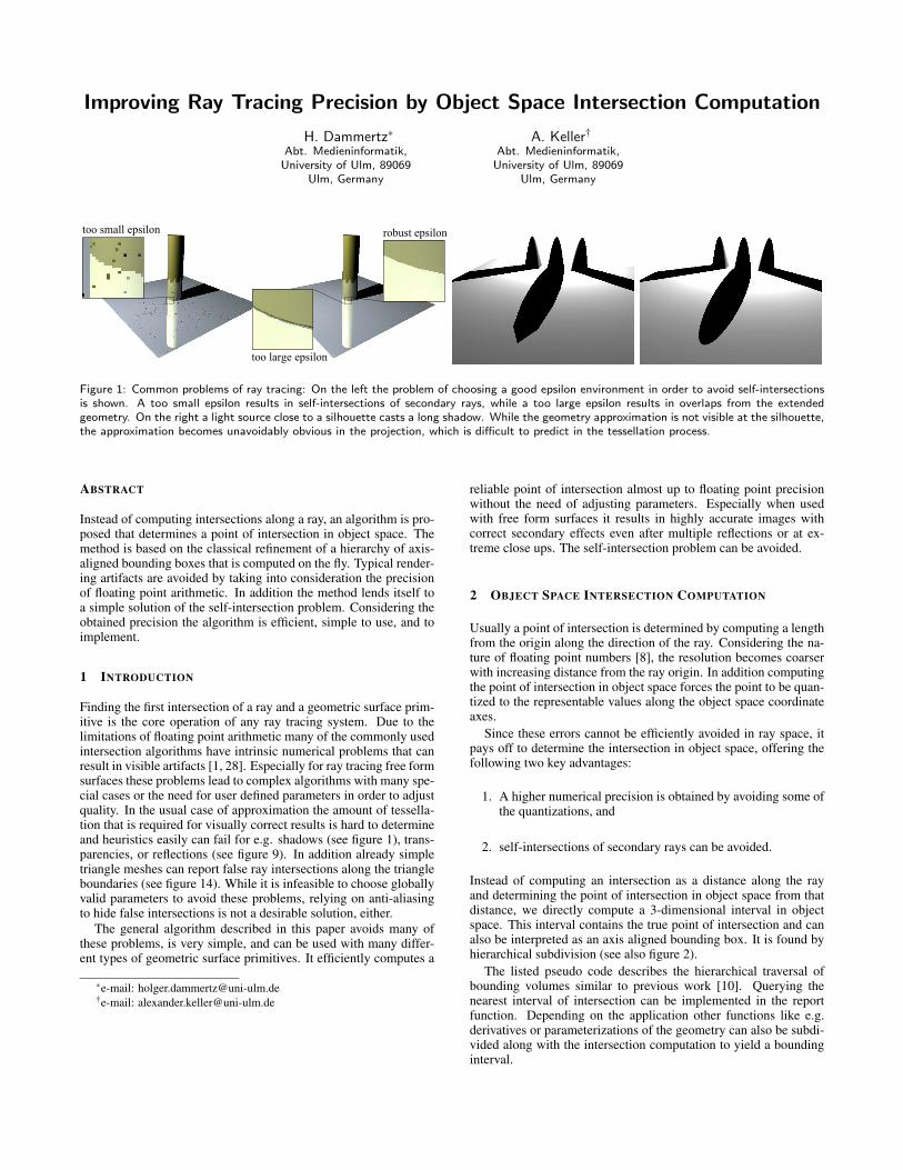
Improving Ray Tracing Precision by Object Space Intersection Computation H. Dammertz * Abt. Medieninformatik, University of Ulm, 89069 Ulm, Germany A. Keller † Abt. Medieninformatik, University of Ulm, 89069 Ulm, Germany Figure 1: Common problems of ray tracing: On the left the problem of choosing a good epsilon environment in order to avoid self-intersections is shown. A too small epsilon results in self-intersections of secondary rays, while a too large epsilon results in overlaps from the extended geometry. On the right a light source close to a silhouette casts a long shadow. While the geometry approximation is not visible at the silhouette, the approximation becomes unavoidably obvious in the projection, which is difficult to predict in the tessellation process. ABSTRACT Instead of computing intersections along a ray, an algorithm is pro- posed that determines a point of intersection in object space. The method is based on the classical refinement of a hierarchy of axis- aligned bounding boxes that is computed on the fly. Typical render- ing artifacts are avoided by taking into consideration the precision of floating point arithmetic. In addition the method lends itself to a simple solution of the self-intersection problem. Considering the obtained precision the algorithm is efficient, simple to use, and to implement. 1 I NTRODUCTION Finding the first intersection of a ray and a geometric surface prim- itive is the core operation of any ray tracing system. Due to the limitations of floating point arithmetic many of the commonly used intersection algorithms have intrinsic numerical problems that can result in visible artifacts [1, 28]. Especially for ray tracing free form surfaces these problems lead to complex algorithms with many spe- cial cases or the need for user defined parameters in order to adjust quality. In the usual case of approximation the amount of tessella- tion that is required for visually correct results is hard to determine and heuristics easily can fail for e.g. shadows (see figure 1), trans- parencies, or reflections (see figure 9). In addition already simple triangle meshes can report false ray intersections along the triangle boundaries (see figure 14). While it is infeasible to choose globally valid parameters to avoid these problems, relying on anti-aliasing to hide false intersections is not a desirable solution, either. The general algorithm described in this paper avoids many of these problems, is very simple, and can be used with many differ- ent types of geometric surface primitives. It efficiently computes a * e-mail: [email protected] † e-mail: [email protected] reliable point of intersection almost up to floating point precision without the need of adjusting parameters. Especially when used with free form surfaces it results in highly accurate images with correct secondary effects even after multiple reflections or at ex- treme close ups. The self-intersection problem can be avoided. 2 OBJECT SPACE I NTERSECTION COMPUTATION Usually a point of intersection is determined by computing a length from the origin along the direction of the ray. Considering the na- ture of floating point numbers [8], the resolution becomes coarser with increasing distance from the ray origin. In addition computing the point of intersection in object space forces the point to be quan- tized to the representable values along the object space coordinate axes. Since these errors cannot be efficiently avoided in ray space, it pays off to determine the intersection in object space, offering the following two key advantages: 1. A higher numerical precision is obtained by avoiding some of the quantizations, and 2. self-intersections of secondary rays can be avoided. Instead of computing an intersection as a distance along the ray and determining the point of intersection in object space from that distance, we directly compute a 3-dimensional interval in object space. This interval contains the true point of intersection and can also be interpreted as an axis aligned bounding box. It is found by hierarchical subdivision (see also figure 2). The listed pseudo code describes the hierarchical traversal of bounding volumes similar to previous work [10]. Querying the nearest interval of intersection can be implemented in the report function. Depending on the application other functions like e.g. derivatives or parameterizations of the geometry can also be subdi- vided along with the intersection computation to yield a bounding interval.
Transcript of Improving Ray Tracing Precision by Object Space ... · Improving Ray Tracing Precision by Object...
Improving Ray Tracing Precision by Object Space Intersection Computation
H. Dammertz∗
Abt. Medieninformatik,University of Ulm, 89069
Ulm, Germany
A. Keller†
Abt. Medieninformatik,University of Ulm, 89069
Ulm, Germany
Figure 1: Common problems of ray tracing: On the left the problem of choosing a good epsilon environment in order to avoid self-intersectionsis shown. A too small epsilon results in self-intersections of secondary rays, while a too large epsilon results in overlaps from the extendedgeometry. On the right a light source close to a silhouette casts a long shadow. While the geometry approximation is not visible at the silhouette,the approximation becomes unavoidably obvious in the projection, which is difficult to predict in the tessellation process.
ABSTRACT
Instead of computing intersections along a ray, an algorithm is pro-posed that determines a point of intersection in object space. Themethod is based on the classical refinement of a hierarchy of axis-aligned bounding boxes that is computed on the fly. Typical render-ing artifacts are avoided by taking into consideration the precisionof floating point arithmetic. In addition the method lends itself toa simple solution of the self-intersection problem. Considering theobtained precision the algorithm is efficient, simple to use, and toimplement.
1 INTRODUCTION
Finding the first intersection of a ray and a geometric surface prim-itive is the core operation of any ray tracing system. Due to thelimitations of floating point arithmetic many of the commonly usedintersection algorithms have intrinsic numerical problems that canresult in visible artifacts [1, 28]. Especially for ray tracing free formsurfaces these problems lead to complex algorithms with many spe-cial cases or the need for user defined parameters in order to adjustquality. In the usual case of approximation the amount of tessella-tion that is required for visually correct results is hard to determineand heuristics easily can fail for e.g. shadows (see figure 1), trans-parencies, or reflections (see figure 9). In addition already simpletriangle meshes can report false ray intersections along the triangleboundaries (see figure 14). While it is infeasible to choose globallyvalid parameters to avoid these problems, relying on anti-aliasingto hide false intersections is not a desirable solution, either.
The general algorithm described in this paper avoids many ofthese problems, is very simple, and can be used with many differ-ent types of geometric surface primitives. It efficiently computes a
∗e-mail: [email protected]†e-mail: [email protected]
reliable point of intersection almost up to floating point precisionwithout the need of adjusting parameters. Especially when usedwith free form surfaces it results in highly accurate images withcorrect secondary effects even after multiple reflections or at ex-treme close ups. The self-intersection problem can be avoided.
2 OBJECT SPACE INTERSECTION COMPUTATION
Usually a point of intersection is determined by computing a lengthfrom the origin along the direction of the ray. Considering the na-ture of floating point numbers [8], the resolution becomes coarserwith increasing distance from the ray origin. In addition computingthe point of intersection in object space forces the point to be quan-tized to the representable values along the object space coordinateaxes.
Since these errors cannot be efficiently avoided in ray space, itpays off to determine the intersection in object space, offering thefollowing two key advantages:
1. A higher numerical precision is obtained by avoiding some ofthe quantizations, and
2. self-intersections of secondary rays can be avoided.
Instead of computing an intersection as a distance along the rayand determining the point of intersection in object space from thatdistance, we directly compute a 3-dimensional interval in objectspace. This interval contains the true point of intersection and canalso be interpreted as an axis aligned bounding box. It is found byhierarchical subdivision (see also figure 2).
The listed pseudo code describes the hierarchical traversal ofbounding volumes similar to previous work [10]. Querying thenearest interval of intersection can be implemented in the reportfunction. Depending on the application other functions like e.g.derivatives or parameterizations of the geometry can also be subdi-vided along with the intersection computation to yield a boundinginterval.

I n t e r s e c t ( Ray , O b j e c t ){
bbox = a x i s a l i g n e d bounding box of O b j e c ti f ( Ray m i s s e s bbox )
re turne l s e i f ( t e r m i n a t e )
r e p o r t ( bbox as i n t e r s e c t i o n i n t e r v a l )re turn
e l s e{
sd = s u b d i v i d e O b j e c tf o r ( a l l o b j e c t s o i n sd )
I n t e r s e c t ( Ray , o )}
}
Listing 1: Bounding volume hierarchy traversal.
2.1 Numerically Robust Algorithm
Bounding intervals can be computed by interval or affine arithmetic[10, 13, 4], which is the common means to address floating pointprecision problems. However, each arithmetic operation then hasto be performed in interval or affine arithmetic resulting in a highcomputational effort. Using the key observation that for two float-ing point numbers a 6= b it can happen that (a+b)/2 = a, the over-head of replacing arithmetic operations by operations on intervalscan be avoided: Intervals are subdivided until the subdivision nolonger changes in the floating point representation. For the ray in-tersection with an object this involves:
Numerically robust subdivision: Cracks usually result from dif-ferent levels of subdivision or numerical problems. If theneighboring bounding boxes resulting from subdivision over-lap or at least touch in floating point representation, no cracks,even between different levels of subdivision, can occur. In theapplications section we show how to guarantee this.
Numerically robust termination: Subdivision is terminated if thesize of the resulting bounding boxes no longer is changing infloating point arithmetic. The resulting bounding box then isreported as intersection interval.It is important to select a measure that is robust with respect tothe floating point arithmetic. Computing the Euclidian lengthof the diagonal of a bounding box involves squares. As thebounding boxes tend to become very small by subdivision,cancelation errors [8] would cause too early termination. Wetherefore use the L1-norm of the bounding box diagonal, i.e.the sum of the absolute values. In contrast to the Euclideanlength it only requires subtractions and additions to computeand thus remains more precise.
Fulfilling the above conditions in an implementation of the bound-ing volume hierarchy traversal (see the pseudo code) results ina crack and hole free intersection computation. The decision ofwhether or not a bounding box is intersected by a ray is decidedusing the algorithm of Williams et al. [27]. Seemingly contradic-tory to our goal, although not used for the intersection interval, thismethod uses distances along the ray. Note that we do not have anyother choice as long as the rays are given by origin and direction.However, the computations remain consistent, because for floatingpoint arithmetic the above conditions assure that if a box is inter-sected at a higher level of the hierarchy there exists at least oneof them, which is intersected in the lower levels. This includes thesituation where the floating point resolution along the ray is not suf-ficient to precisely capture the intersection interval in object space.Such a situation arises for a ray far from the origin targeting at anobject close to the origin.
2.2 Secondary Rays
Realistic image synthesis requires shooting secondary rays in or-der to compute the illumination. The problem of self-intersectionsbecomes apparent (see figure 1), when shooting off rays from sur-faces: Due to numerical inaccuracies the same surface may be hitagain, resulting in false points of intersection. A common solutionto this problem is adding a small distance along the ray or normaldirection. The choice of this epsilon is largely scene dependent andoften left to the user of the ray tracing system. Using object identi-fications also does not help for non-planar or touching objects.
With the intersection interval computed by our algorithm we canavoid the self-intersection problem. The starting point of the sec-ondary ray is selected as the corner point of the intersection intervalfarthest in the direction of the normal (see the illustration in 3). Fortransparency rays we just use the normal with inverted signs. As avalid ray interval excludes the origin of the ray, it is impossible tohit the interval of origin again.
Figure 3: Avoiding the self-intersection problem by selecting the cor-ner of the intersection interval that is farthest in the direction of thesurface normal.
This method works perfectly in convex geometries. Neverthe-less, an epsilon environment is required, to avoid early intersec-tions of close to tangential rays in concave geometry. But this canbe done globally without user interaction. The intersection intervalis enlarged by considering its binary representation of the floatingpoint number as integer [11]. In our implementation we subtract /add the value of 7 (3 bits). This way the epsilon value is implicitlyadapting to the exponent of the floating point number. It has beenfound by comparing single and double precisions computation.
3 APPLICATIONS
We demonstrate the general algorithm for three applications,namely polynomial free form surfaces, trimming, and improved tri-angle intersection testing. The speed of the algorithms is interac-tive, however, as we focus on precision, might be inferior to moreapproximative schemes.
3.1 Polynomial Free Form Surfaces
The approaches to ray tracing free form surfaces can be roughlyclassified into three different strategies: First the surface can be ap-proximated by simpler surfaces. Often planar polygons or bilinearpatches are used for the approximation. However, this eventuallyresults in the problems illustrated in figures 1, 9, and 14.
Secondly, there are subdivision based algorithms that use a sim-ple prune and search method. Early methods are described by Whit-ted [26] and Rubin [22]. Woodward [29] transforms the problem totwo dimensions. Nishita et al. [19] developed the well known tech-nique of Bezier clipping, which has been improved in [3]. Anothersubdivision based method called Chebyshev boxing is described in[6]. Recent work on subdivision based methods can be found in[18, 2].

Figure 2: Illustration of the hierarchical refinement of the bounding boxes as used in the algorithm. Instead of ray parameters bounding boxesthat contains the actual points of intersection are determined directly.
The third category comprises numerical solutions, where a formof Newton iteration is used in most cases to find the point of inter-section. All methods based on simple Newton iteration [7, 16] havethe problem of finding a good starting point and the user has to se-lect parameters to obtain a correct image (see figure 4). Kajiya [14]uses algebraic geometry to create a numerical procedure for find-ing the intersection between a ray and a bivariate cubic parametricpatch. A more accurate approach is described by Toth [23] and im-proved in [15]. It uses multivariate Newton iteration to solve theconvergence problem of Newton iteration but this method is ratherslow.
All the above methods suffer from disadvantages like coarse ap-proximations, numerical problems, extensive computation, param-eters that are difficult to determine for an overall scene, or restric-tions on subdivision depth and surface degree.
Our method falls into the second category. We now specify thealgorithm from the previous section for polynomial free form sur-faces of arbitrary degree.
Figure 4: False surface intersection reported by Newton iteration,when the starting point is not sufficiently close to the fix point.
3.1.1 Polynomial Tensor Product Surfaces
Using the Bezier representation is one of the simplest ways to de-scribe a polynomial surface. Even though it is not well suited formodeling purposes any polynomial surface can be converted intothe Bezier basis (NUBS surfaces for example by knot insertion [20]- it is not NURBS, since it is not rational). For the remainder of thisdiscussion we assume familiarity with Bezier surface patches [5].
A Bezier surface patch
p(u,v) :=m
∑i=0
n
∑j=0
Bmi (u)Bn
j(v)pi j u,v ∈ [0 . . .1]. (1)
is defined by a two dimensional grid of control points pi j andthe Bernstein basis functions Bk
i (t) of degree k. The axis alignedbounding box of a Bezier patch is computed by taking the mini-mum and maximum of all (n+1)(m+1) control points pi j in eachcomponent.
The subdivision of a Bezier surface patch is done via the deCasteljau algorithm using the recursion property of the Bernsteinbasis. With respect to floating point computations the best parame-ter value for subdivision is 0.5. This guarantees that the boundaries
of the intersection intervals always touch and no cracks can appearas required in section 2.1. In addition the division by 2 is just adecrement of the exponent and is always exact unless a floatingpoint underflow occurs [8].
The selection of the subdivision is guided by a simple heuristic.It estimates the longest direction by computing the length of thetwo vectors (pn,0 − p0,0) and (p0,m − p0,0) and subdivides alongthe longer direction. The norm used to determine the length onlyaffects the efficiency of the scheme. Therefore, we use the max-imum norm, which can be evaluated fastest. The heuristic workseven for very distorted self-intersecting patches of high degree asshown in figure 6, because the resulting patches become very regu-lar after only a few subdivisions.
3.1.2 Accuracy
To analyze the accuracy obtained by our subdivision algorithm, werounded the results of an implementation using double precisionarithmetic to the nearest single precision number. These were com-pared to the actual single precision version and the results of a uni-form triangulation of the patch. The triangle intersection algorithmused is the one described in [17]. Its intersection point was com-pared to the midpoint of the intersection interval of our method.Figure 8 shows the two patches that were used. The results canbe found in tables 1 and 2. It becomes obvious that tessellation ap-proaches like e.g. [2] result in larger approximation errors. Even forhigh tessellations our subdivision intersection algorithm performsbetter by two orders of magnitude.
The errors obtained by interpolating normals of triangle cornersand direct computation are very similar. This can be clearly seen inthe reflections in figure 9.
Figure 6: Two ray traced Bezier patches (left: degree 10 in u anddegree 7 in v direction, right: random control points and degree 42in both u and v direction) demonstrating robustness of the algorithmfor high degrees. Finding stable starting points for Newton iterationbecomes almost impossible in this setting.

Figure 5: A NURBS scene converted into 261692 Bezier patches and ray traced with our algorithm.
3.1.3 Speed of Convergence
The subdivision of a Bezier patch can be implemented efficientlyusing the vector instructions of modern computer architecture (see[2] for example). A simple and straightforward implementation waschosen for the analysis. The subdivision and bounding box compu-tation was implemented using SSE instructions but only 3 of the 4slots were used. The reason for the good performance of our algo-rithm is that it completely runs in the level 1 cache of the processor.As such it is compute-bound.
Figure 7: A Bezier patch with the color encoded number of subdivi-sions needed to determine the intersection interval. Green is about50 subdivisions, yellow up to 200 and red more than 200 subdivisions.
The first interesting thing about the algorithm is the number ofsubdivisions needed until an intersection interval is found. As canbe seen in figure 7, the effort needed to determine the intersectioninterval grows the more the ray direction tangential to the surface.Note that the same effect would be observed for tessellations. Thereason for this is an increased number of bounding boxes that haveto be intersected when the ray passes almost parallel to the surface.Furthermore the number of iterations needed to find an intersectioninterval depends on the size of the patch and its position in 3d space.Due floating point arithmetic larger patches and patches that areclose to the origin take longer to ray trace [8]. For the analysisall patches were contained in [1,2]3. We provide this interval forreference.
The control polygon of a Bezier surface converges quadraticallyto the surface when the de Casteljau subdivision is used [21]. Con-
sequently we have the same rate of convergence for the boundingbox of the control polygon, too.
Figure 8: The two patches used for the accuracy analysis. The imageshows the difference between the patch tesselated to 512 trianglesand the single precision subdivision algorithm.
# Tris Max. Error Min. Error Mean Error512 3.0642e−1 4.4703e−8 4.9815e−3
4608 8.5224e−2 8.4750e−8 5.5706e−4131072 2.7960e−3 0.0000e+0 1.9592e−5
our Alg. 8.5681e−5 0.0000e+0 2.3038e−7
Table 1: Point of intersection error for a simple patch (figure 8 onthe left) compared to the double precision results.
3.1.4 Performance
The algorithm for ray tracing Bezier patches was integrated intoa simple ray tracing system that also allows ray tracing of trian-gle models and has support for hierarchical materials and differentlight sources. The triangle ray tracer uses kD-trees for each objectas acceleration structure. A top level axis aligned bounding volumehierarchy (BVH) is used to support instances and multiple objects.The Bezier ray tracer uses the BVH for top level and for individ-ual objects. The test scenes are completely composed of NURBSpatches and were ray traced at a resolution of 512x512 pixels with

# Tris Max. Error Min. Error Mean Error512 1.8080e+0 5.9604e−8 9.5757e−3
4608 4.0562e−1 0.0000e+0 1.1005e−3131072 1.1100e−2 0.0000e+0 3.8533e−5
our Alg. 9.3240e−5 0.0000e+0 2.2959e−7
Table 2: Point of intersection error for a more distorted patch. Thepatch can be seen in figure 8 on the right.
Figure 9: The scene on the left was triangulated into 10752 triangles.The discontinuities of the first derivative are clearly visible in thereflections of the bars. The image on the right was ray traced withthe subdivision algorithm. The resolution of both images is 512x512.
one primary ray per pixel. The ray tracing was done on a Pen-tium 4 at 2.8 GHz with 2GB of RAM and the ray tracers used onlya single thread. The conversion of the NURBS patches into inte-gral Bezier patches needed no approximation in this case becauseof the modeling program Alias Maya 5.0, which generates rationalsurfaces only in rare cases. The adaptive conversion algorithm inte-grated into Alias Maya 5.0 was used to create the tessellation. Twotest scenes were used for comparison. The dog scene has a simpleLambertian material and only primary rays were traced. The carscene features highly reflective materials. The recursion depth wasset to 3 for reflections and 6 for refractions. The scene contains29 different materials and 9 point light sources. The results areshown in figure 10. The memory consumption is the scene geom-etry plus the acceleration data structure size. The parse time is thetime for reading and interpreting the scene description supported byour rendering system. The render time is the time for accelerationdata structure construction and ray tracing a single image. Giventhe superior precision of our algorithm, it is very competitive.
3.1.5 Optimizations
There are various possibilities to increase the performance of thebasic algorithm. Since the intersection computation dominates therendering time, optimization of the intersection calculation is mostimportant. Obvious improvements are iterative implementation ofsubdivision using a simple stack instead of a recursive implemen-tation and organizing the data in processor friendly structures andalignments. A huge improvement in subdivision performance canbe gained by subdividing the data of a patch in place, overwritingthe original patch on the stack. This reduces memory access andallows for better register usage. Another improvement is travers-ing the subdivided bounding box that is closer to the ray first. Thisincreases the likelihood of an early termination during the subdivi-sion.
A common principle to accelerate the tracing of primary rays isto use coherent packets of rays as described for example by Waldin [25]. However, since bounding boxes are subdivided almost upto the resolution of floating point number, ray coherency is lost andbundle tracing as well as shaft culling [9] does not help much (see
table 3).Using coherent rays for the higher levels of the hierarchy is help-
ful. This corresponds to truncating accuracy. Instead of using thetermination criterion as described in section 2.1, we allow early ter-mination. For example the subdivision can be stopped when thesize of the bounding box projected to the screen is smaller than halfa pixel. When no secondary rays are traced the resulting imagesare equivalent to the images computed with the floating point ter-mination criterion. For secondary rays, ray differentials [12] couldbe used, but this has not been examined yet. Table 3 shows someperformance data for a single patch.
#Rays in Bundle Float Acc. Early Term.1x1 0.567 fps 1.266 fps2x2 0.657 fps 1.996 fps4x2 0.676 fps 2.236 fps2x4 0.680 fps 2.280 fps4x4 0.640 fps 2.395 fps8x8 0.297 fps 0.530 fps
Table 3: Performance when using ray bundles of different size. Theperformance data was collected at a resolution of 512x512 with thepatch shown in figure 7
3.2 Trimming Curves
Trimming can be used to overcome the topological restriction oftensor product surfaces. For this, a hierarchy of polynomial curvesuniquely defines inside and outside points in the parameter domainof the patch. These polynomial curves can be converted into Bezierrepresentation and inside and outside points can be identified by raytracing, using Jordan’s curve theorem . This is done by shooting aray into an arbitrary direction and counting all intersections with thecurves. Odd and even numbers of intersections distinguish insidefrom outside.
Figure 11: The four different cases for a single curve segment thatcan occur during the trimming test.
Since the test is arbitrary, we select the positive u-axis, whichsimplifies the implementation. Besides the reduction of the previ-ous techniques to two dimensions, we only want to know whetherthe number of all intersections is even or odd. Transferring theprinciples of the previous section allows for an efficient trimmingalgorithm that achieves almost floating point precision.
We briefly sketch the algorithm that works for arbitrary degreealong the lines of [19]. Figure 11 shows the four different cases thealgorithm has to consider:
Cases 1 and 2: If all control points of the curve segment, i.e. the

Scene # of Primitives Parse Time Memory Render TimeDog Triangles 422122 11.5 16.89MB 1.318sDog Bezier 24878 0.7s 6.47MB 3.283sCar Triangles 1505118 252.4s 303MB 2573.4sCar Bezier 261692 12.2s 29MB 812.6s
Figure 10: Performance of the Bezier subdivision algorithm compared to a triangle ray tracer. Given the superior precision of our algorithm, itis very competitive.
bounding box, lie left of the v-axis or above/below the u-axis,the ray does not intersect.
Case 3: The curve is on the right side of the v-axis but neitherabove nor below the u-axis. If the two endpoints of the curveare on the same side (above or below the u-axis), the ray in-tersects the curve an even number of times. Otherwise thenumber is odd. This is due to the continuity of polynomialcurves.
Case 4: Now we have to recursively subdivide using the L1 termi-nation criterion. Upon termination we assume an intersection.
Figure 12: A trimmed Bezier patch. On the right the color encodedeffort for trimming is shown. On average trimming is about 50% ofthe total intersection cost.
Figure 13: Quadrisection of a triangle using stable subdivision byedge midpoints.
3.3 Triangles
The principles developed so far can be used to avoid self-intersection problems (see section 2.2) and holes in triangularscenes. It is important to note that changing to double precisionor different triangle tests does not avoid holes. Even the Pluckertest, which avoids holes along edges, can fail around the vertices ofthe geometry.
Subdividing each triangle edge in the middle (see figure 13 and[24]) already fulfills the numerical requirements of section 2.1. Infact a triangle can be considered as a triangular planar Bezier patchand thus the results of section 3.1 apply.
Figure 14 shows the happy Buddha mesh. The image was raytraced at a resolution of 512x512 pixels using the triangle test of
Figure 14: The happy buddha mesh with 1087716 triangles. Whenray traced with standard triangle intersection algorithms false inter-sections can be reported. This problem does not occur with oursubdivision algorithm.
Moller and Trumbore [17]. While 3.64 frames per second are ob-tained, some false intersections are reported along triangle edges.Using the stable algorithm avoids these errors and results in 0.73frames per second.
If the intersection interval is not required to avoid self-intersections and only a hole free rendering is desirable, we canspeed up computations by using our algorithm whenever a cheapertriangle test ([17] in our case) reports no intersection. Then the per-formance increases from 0.73 fps to 2.24 fps for the Buddha mesh.
4 CONCLUSION AND FUTURE WORK
We have presented an algorithm that generally increases the pre-cision of ray tracing without ad-hoc parameter adjustments. Theresults are especially interesting for precise simulation and produc-tion rendering.
Future work comprises finding a similar stable termination cri-terion that could be used for rational surfaces. First experimentshave shown that ignoring the last few bits of the L1-norm in the ter-mination criterion produces good results. Until now there are onlyempirical results for the number of bits to ignore and they vary de-pending on the surface degree. Our algorithm can be used for manydifferent kinds of subdivision surfaces. First implementations withLoop and Catmull-Clark surfaces have produced good results. Sim-ilar to the problems of rational surfaces, we still explore problems

with the subdivision accuracy at irregular vertices. Another prob-lem is the performance when subdividing subdivision surfaces onthe fly because of the many special cases that have to be consideredsuch as boundary and irregular vertices.
ACKNOWLEDGEMENTS
We would like to thank Ingo Wald for the fruitful scientific discus-sion.
REFERENCES
[1] J. Amanatides and D. Mitchell. Some regularization problems in raytracing. In Proc. Graphics Interface ’90, pages 221–228, 1990.
[2] C. Benthin, I. Wald, and P. Slusallek. Interactive ray tracing of free-form surfaces. In Proceedings of Afrigraph 2004, pages 99–106,November 2004.
[3] S. Campagna and P. Slusallek. Improving Bezier Clipping and Cheby-shev Boxing for Ray Tracing Parametric Surfaces, 1996.
[4] L. de Figueiredo and J. Stolfi. Affine arithmetic: Concepts and appli-cations, Numerical Algorithms 37 1-4. 2003.
[5] J. Foley, A. van Dam, S. Feiner, and J. Hughes. Computer Graphics:Principles and Practice, 2nd ed. Addison Wesley, 1996.
[6] A. Fournier and J. Buchanan. Chebyshev polynomials for boxing andintersections of parametric curves and surfaces. Computer GraphicsForum, 13(3):127–142, 1994.
[7] M. Geimer and O. Abert. Interactive ray tracing of trimmed bicu-bic Bezier surfaces without triangulation. In WSCG 2005 ConferenceProceedings, Plzen, Czech Republic, 2005.
[8] D. Goldberg. What every computer scientist should know aboutfloating-point arithmetic. ACM Computing Surveys, 23(1):5–48, 1991.
[9] V. Havran. Heuristic Ray Shooting Algorithms. PhD thesis, CzechTechnical University, Praha, Czech Republic, April 2001.
[10] W. Heidrich and H. Seidel. Ray-tracing procedural displacementshaders. In Graphics Interface, pages 8–16, 1998.
[11] M. Herf. Robust epsilons in floating point, http://www.stereopsis.com/robusteps.html, 2000.
[12] H. Igehy. Tracing ray differentials. In Alyn Rockwood, editor, Sig-graph 1999, Computer Graphics Proceedings, pages 179–186, 1999.
[13] A. Junior, L. de Figueiredo, and M. Gattas. Interval methods forraycasting implicit surfaces with affine arithmetic, XII SIBGRAPHI,pages 1-7. 1999.
[14] J. Kajiya. Ray tracing parametric patches. ACM SIGGRAPH Com-puter Graphics, 16(3):245–254, July 1982.
[15] D. Lischinski and J. Gohczarowski. Improved techniques for ray trac-ing parametric surfaces. The Visual Computer, 6(3):134–152, 1990.
[16] W. Martin, E. Cohen, R. Fish, and P. Shirley. Practical ray tracingof trimmed NURBS surfaces. Journal of Graphics Tools, 5(1):27–52,2000.
[17] T. Moller and B. Trumbore. Fast, minimum storage ray-triangle inter-section. Journal of Graphics Tools, 2, 1997.
[18] K. Muller, T. Techmann, and D. Fellner. Adaptive ray tracing of sub-division surfaces. Computer Graphics Forum, 22(3):553–562, 2003.
[19] T. Nishita, T. Sederberg, and M. Kakimoto. Ray tracing trimmed ratio-nal surface patches. Computer Graphics, ACM, 4(24):337–345, 1990.
[20] L. Piegl and W. Tiller. The NURBS Book. Springer, 1997.[21] H. Prautzsch, W. Boehm, and M. Paluszny. Bezier and B-Spline Tech-
niques. Springer, 2002.[22] S. Rubin and T. Whitted. A 3-dimensional representation for fast ren-
dering of complex scenes. ACM SIGGRAPH Computer Graphics,14(3):110–116, July 1980.
[23] D. Toth. On ray tracing parametric surfaces. ACM SIGGRAPH Com-puter Graphics, 19(3):171–179, 1985.
[24] D. Voorhies and D. Kirk. Ray - triangle intersection using binaryrecursive subdivision. In James Arvo, editor, Graphics Gems II, pages257–263. Academic Press, 1991.
[25] I. Wald. Realtime Ray Tracing and Interactive Global Illumination.PhD thesis, Computer Graphics Group, Saarland University, 2004.
[26] T. Whitted. An improved illumination model for shaded display. Com-munications of the ACM, 23(6):343–349, June 1980.
[27] A. Williams, S. Barrus, R. Morley, and P. Shirley. An efficient androbust ray-box intersection algorithm. Journal of Graphics Tools,10(1):49–54, 2005.
[28] A. Woo, A. Pearce, and M. Ouellette. It’s really not a rendering bug,you see... IEEE Computer Graphics & Applications, 16(5):21–25,September 1996.
[29] C. Woodward. Ray tracing parametric surfaces by subdivision in view-ing plane. Theory and Practice of Geometric Modeling, Springer-Verlag New York, Inc., pages 273–287, 1989.