Improving Production Planning and Scheduling

at AC

Master thesis

Version 1.3 (public)March 27, 2012

Student:J. van Twist

Supervisors:prof. dr. ir. W.P.M. Nuijtenir. J.W.M. Welberg

ii

Preface

This master thesis concludes my graduation project performed during my study of BusinessInformation Systems at Eindhoven University of Technology (TU/e). This project is thesecond phase of a larger research project performed in collaboration between TU/e andAC. I highly valued the contribution of several people and I would like to thank them.

First of all, I like to thank my predecessor Roel Coset, who started the first phase of theproject. His clear process description and explanation of the organizational context of AC,got me going very quickly. Also his initial result and future work suggestions provided asolid foundation to build upon. I like to thank my graduation supervisor Wim Nuijten,for the guidance and confidence in the project, and for the provided feedback. I also reallyappreciated his effort to provide work opportunities after this project. I like to thank mysupervisor at AC, Jan-Willem Welberg, for finding the time to provide me with detailedfeedback and (corrections to) many essential input data. His patience, provided flexibility,and arranged meetings greatly contributed to the result of the project. Furthermore, Ithank everyone else at AC who contributed to the project and/or their showed interest.

Finally I like to thank my parents for their support during the project and my friends forthe great time during my study at TU/e.

Joost van TwistEindhoven, march 2012

iii

iv

Abstract

In this document, several improvements to an initially proposed solution of a planning andscheduling problem are identified. This challenging problem is found in the productionprocess of AC1, being the global leader in its product field. The initially proposed solution,given in the form of an automated planning tool, showed promising results of a potentialcost reduction regarding the product availability for sales. However, within the originalplanning tool, two manual post processing steps were required to obtain a solution thatwas competitive with the manual production plans. Furthermore, the initial solutionperformed worse regarding the maintenance of stock levels and the amount of productionchangeovers that were required.

The found improvements mostly involve adaptations made to the original planning tool.Furthermore, many adaptations to the input data and refinements of the constraints (thatrestricted the planning solutions), are applied. The new performance evaluation shows aneven larger cost reduction regarding the product availability for sales. Also, product stocklevels are now maintained better than within the manual production plans. On top of thatit follows that the two manual post processing steps, required for the original planningtool, are not required anymore.

To increase the confidence in the current planning solution several validation experi-ment are conducted. A drawback still present in the current solution is the incrementof changeover costs in the solutions of the planning tool. Although it is the case that min-imization of changeovers does not minimize the other cost objectives, the current planningtool is shown unable to find the minimum amount of changeovers. This even holds afterthe implementation of a post processing step that decreases the amount of changeoversgenerated by the planning tool. To be able to use the planning solution for the comparisonof several what-if scenarios, it is shown that many evaluations of the same scenario haveto be compared, in order to make reliable predictions.

1The name of the company is anonymized in this public version of the document, to protect confidentialinformation.

v

vi

Contents

1 Introduction 3

2 Literature 52.1 Classification of scheduling problems . . . . . . . . . . . . . . . . . . . . . . 52.2 Optimization models . . . . . . . . . . . . . . . . . . . . . . . . . . . . . . . 7

3 Problem description 153.1 Problem description . . . . . . . . . . . . . . . . . . . . . . . . . . . . . . . 153.2 Mathematical model . . . . . . . . . . . . . . . . . . . . . . . . . . . . . . . 16

4 Implementation 254.1 Intermediate data model . . . . . . . . . . . . . . . . . . . . . . . . . . . . . 254.2 PPO’s data model . . . . . . . . . . . . . . . . . . . . . . . . . . . . . . . . 264.3 Mapping . . . . . . . . . . . . . . . . . . . . . . . . . . . . . . . . . . . . . . 264.4 Objectives . . . . . . . . . . . . . . . . . . . . . . . . . . . . . . . . . . . . . 27

5 Improvements 295.1 Rounding error . . . . . . . . . . . . . . . . . . . . . . . . . . . . . . . . . . 295.2 Inventory deficit cost . . . . . . . . . . . . . . . . . . . . . . . . . . . . . . . 305.3 Simultaneous optimization of non-delivery and inventory deficit costs . . . . 305.4 Shunt line constraints . . . . . . . . . . . . . . . . . . . . . . . . . . . . . . 315.5 Evaluation . . . . . . . . . . . . . . . . . . . . . . . . . . . . . . . . . . . . . 325.6 Automatic post processing steps . . . . . . . . . . . . . . . . . . . . . . . . 32

6 Evaluation 376.1 Verification manual planning . . . . . . . . . . . . . . . . . . . . . . . . . . 376.2 Validation . . . . . . . . . . . . . . . . . . . . . . . . . . . . . . . . . . . . . 396.3 Analysis . . . . . . . . . . . . . . . . . . . . . . . . . . . . . . . . . . . . . . 39

7 Conclusion 437.1 Future work . . . . . . . . . . . . . . . . . . . . . . . . . . . . . . . . . . . . 44

Bibliography 51

1

2

Chapter 1

Introduction

Even though a large amount of research is conducted in the area of production planningand scheduling, still very challenging problem variants exist. Such an instance is foundin the production planning and scheduling process of AC. To improve and support thisprocess, an initial proposed solution has been suggested in the form of an automatedplanning tool by [4]. The work of [4] was the initial step in a larger research project byTU/e and AC as partner. This graduation project is the second phase and aims to furtherinvestigate the potential of the initially proposed solution and to possibly identify severalimprovements. Some of these improvements were already suggested by [4].

For more information about the organizational context of AC and the background ofthe planning problem, the reader is referred to the work of [4]. Also, an overview of theresearch done in the area of planning and scheduling is given by [4] and is extended here inChapter 2. The planning problem at AC was mathematically formalized by [4] and foundto be of large complexity. A drawback of this description is that it is based on solvinga planning problem (assigning productions to fixed buckets). One potential improvementis to base the problem description on solving a scheduling problem that is more tailoredtowards the actual problem that is solved. This type of problem description and a recapof the textual problem description is given in Chapter 3.

The relevant optimization criteria for the suggested solution can be found in Section 3.2.4.A comparison of the model output with the manual planning by [4] suggested a potentialimprovement of 17% in the non-delivery costs, however with an increase of the inventorydeficit costs and the setup costs. On top of that two manual post processing steps wererequired on the generated schedules by the model. In Chapter 5, several improvementsare identified that remove the necessity of these post processing steps. Also, the initialevaluation given in Chapter 5 shows that all cost objectives are reduced compared to theoriginal model of [4]. Furthermore, two automatic post processing steps (Section 5.6) aredesigned to improve the quality of the generated schedules by the model.

Other improvements involve changes to the technical constraints and fixing errors in theinput data of the model. As can be seen in the updated problem description in Chapter 3,some technical constraints have been added, whereas others have been removed, comparedto the initial model of [4]. Due to the large amount of changes in the model, a newimplementation description of the current model is given in Chapter 4. A final evaluationstudy has been conducted to measure the quality of the current model in Chapter 6. Thisis followed by a conclusion and a suggestion for future work in Chapter 7.

3

4

Chapter 2

Literature

The objective of production planning is to be able to fulfill customer demand for a givenset of time periods. This involves the allocation of various resources within the productionfacility over a time period generally covering a few weeks to a few months. This type ofplanning is also referred to as medium-term scheduling in literature. Long-term productionplanning on the other hand involves actual changes to the supply chain, such as facilitylocations. Short-term scheduling is in general more detailed and provides a productionschedule on a short time horizon covering several days to minutes. The main issue is todecide when, where, and how to produce a set of items given a set of various processingrecipes. Scheduling can have lots of different objectives such as minimizing makespan,minimizing earliness/tardiness costs and maximizing profit [8]. Since the boundaries ofplanning and scheduling problems are not well established and there is an intrinsic in-tegration between these decision making stages, there is a lot of work in the literatureaddressing the simultaneous consideration of planning and scheduling decisions [28]. Also,batching decisions (i.e., the number and size of batches) are often treated as planningdecisions (and thus provided to the scheduling problem), but can also be viewed as partof the scheduling problem [20]. Another thin boundary in literature is between the use ofthe terms resource and unit. A resource is usually a physical material or equipment witha certain capacity. Units on the other hand are mostly the main producing machines andcan perform one task at the time. Units can be viewed as resources modeling wise (bygiving them a capacity of 1) and hence the term unit is often used together with the termresource. The purpose of chapter is to give an overview of the research done in planningand scheduling in the batch process industry and hereby highlighting some of the recentdevelopments covering the last few years.

2.1 Classification of scheduling problems

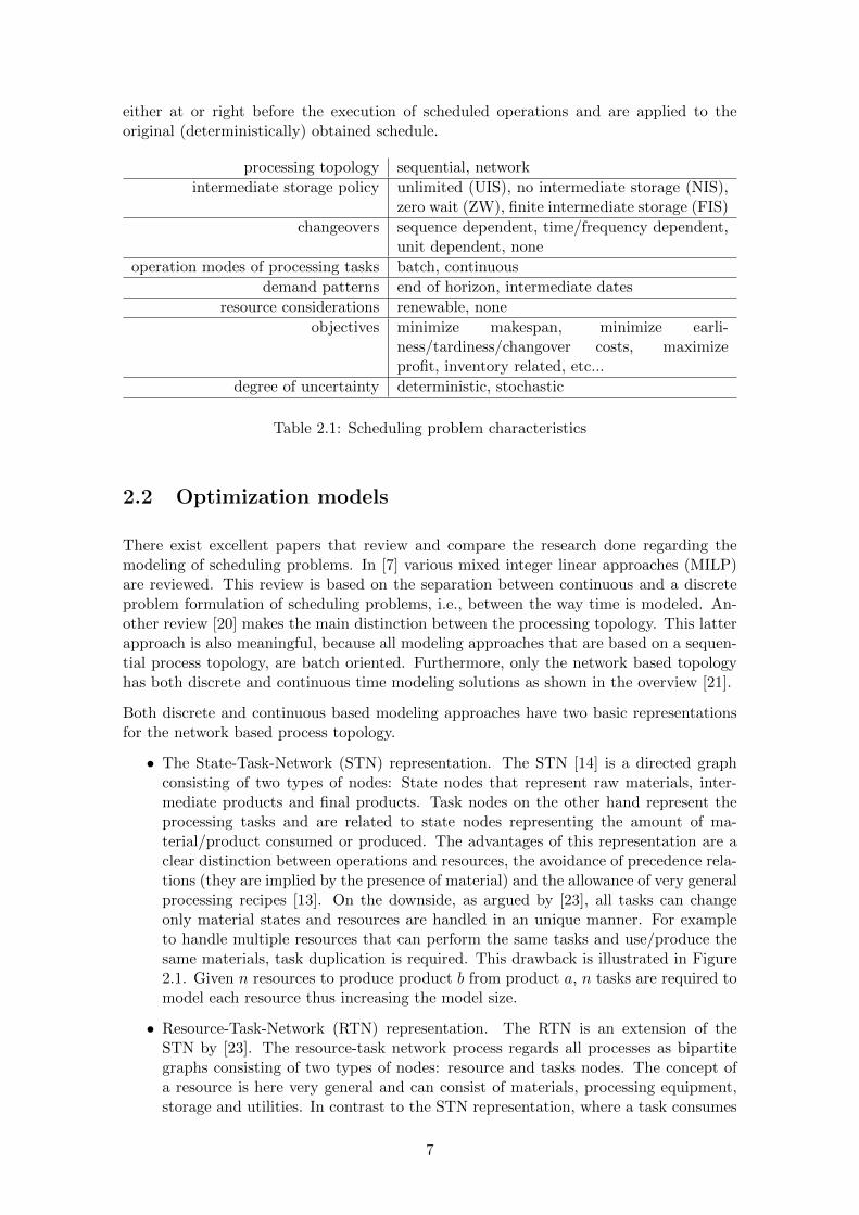
The classification of scheduling problems shows that there is a tremendous diversity offactors that must be accounted for, which makes the task of developing unified generalmethods quite difficult [21]. Table 2.1 gives an overview of the various characteristics.This overview shows that there are many different combinations possible of schedulingproblems in practice. An important feature here is the process topology:

• Sequential processes consist either of a single stage or multiple stages. Within thesetype of processes, batches are used to represent production, thus it is not necessaryto consider mass balances explicitly. Two different types of plants are distinguishedhere: Multiproduct plants produce multiple products following a sequential similar

5

recipe. Multipurpose plants however, consist of general purpose equipment (re-sources) used to manufacture a variety of products, where each product can havedifferent task structures and equipment requirements. This difference is illustratedin Figure 2.1. The scheduling for multipurpose plants is hence significantly moredifficult that that of multiproduct plants [24].

• In networked processes the topology is of arbitrary structure and the network pro-cesses are a mix of convergent and divergent flow paths. Hence material balancesare required to be taken into account explicitly. It involves the splitting and mixingof batches and the use of complex processing recipes.

product A

product B

product C

stage 1 stage 2 stage 3

(a) Multiproduct

stage A

stage D

stage C

stage B

stage E

product A

product B

product C

(b) Multipurpose

Regarding the processing tasks two types are distinguished: Batch tasks and continuoustasks. Batch tasks have a fixed duration and batch size. Furthermore the final productis produced/delivered in it’s entirety at the end of the tasks execution. Continuous tasks,however, usually have a fixed processing rate and sometimes can have a minimum ormaximum bound to either the processing rate or the minimum and maximum duration ofthe task. On top of that the products being produced are added to the stock during thetasks execution instead of at the tasks ending time.

The produced materials and products may be stored according to different policies. Un-limited intermediate storage (UIS) means that produced goods may stay in the inventoryfor infinite time without being consumed. If this duration is limited, because for examplethe goods spoil after some time, a finite intermediate storage (FIS) is applied. It mightbe the case that produced material require to be consumed immediately after productionand then a zero wait (ZW) policy is maintained. If there is no intermitted storage at all(NIS), this means subsequent tasks that produce and consume the same material can beseen as one task.

Produced products might require to be delivered during the manufacturing process. Thismeans that scheduling also needs to determine when to deliver which products and inwhat quantity, besides when and how to produce them. The demand of all products caneither be at the end of the scheduling horizon or at intermediate due dates. In some casesdue dates are given in terms of a window having a minimum and/or maximum deliverytime. In this case earliness and tardiness costs can be introduced as well in the objective,if orders are delivered too early or too late respectively.

In the last decade a new feature of scheduling problems that gets studied, is the degreeof uncertainty within production scheduling. Namely, in practise many of the parametersthat are associated with scheduling are not known exactly. Parameters like raw materialavailability, prices, machine reliability, and market requirements vary with respect to timeand are often subject to unexpected deviations [16]. The work in [16] provides an analysison the sources of uncertainty in process scheduling and also gives an overview of thedifferent modeling solutions dealing with these various unknown parameters. Adjustingthe schedule upon realization of these uncertain parameters or occurrences of unexpectedevents is called reactive scheduling. The reactive scheduling corrections are performed

6

either at or right before the execution of scheduled operations and are applied to theoriginal (deterministically) obtained schedule.

processing topology sequential, network

intermediate storage policy unlimited (UIS), no intermediate storage (NIS),zero wait (ZW), finite intermediate storage (FIS)

changeovers sequence dependent, time/frequency dependent,unit dependent, none

operation modes of processing tasks batch, continuous

demand patterns end of horizon, intermediate dates

resource considerations renewable, none

objectives minimize makespan, minimize earli-ness/tardiness/changover costs, maximizeprofit, inventory related, etc...

degree of uncertainty deterministic, stochastic

Table 2.1: Scheduling problem characteristics

2.2 Optimization models

There exist excellent papers that review and compare the research done regarding themodeling of scheduling problems. In [7] various mixed integer linear approaches (MILP)are reviewed. This review is based on the separation between continuous and a discreteproblem formulation of scheduling problems, i.e., between the way time is modeled. An-other review [20] makes the main distinction between the processing topology. This latterapproach is also meaningful, because all modeling approaches that are based on a sequen-tial process topology, are batch oriented. Furthermore, only the network based topologyhas both discrete and continuous time modeling solutions as shown in the overview [21].

Both discrete and continuous based modeling approaches have two basic representationsfor the network based process topology.

• The State-Task-Network (STN) representation. The STN [14] is a directed graphconsisting of two types of nodes: State nodes that represent raw materials, inter-mediate products and final products. Task nodes on the other hand represent theprocessing tasks and are related to state nodes representing the amount of ma-terial/product consumed or produced. The advantages of this representation are aclear distinction between operations and resources, the avoidance of precedence rela-tions (they are implied by the presence of material) and the allowance of very generalprocessing recipes [13]. On the downside, as argued by [23], all tasks can changeonly material states and resources are handled in an unique manner. For exampleto handle multiple resources that can perform the same tasks and use/produce thesame materials, task duplication is required. This drawback is illustrated in Figure2.1. Given n resources to produce product b from product a, n tasks are required tomodel each resource thus increasing the model size.

• Resource-Task-Network (RTN) representation. The RTN is an extension of theSTN by [23]. The resource-task network process regards all processes as bipartitegraphs consisting of two types of nodes: resource and tasks nodes. The concept ofa resource is here very general and can consist of materials, processing equipment,storage and utilities. In contrast to the STN representation, where a task consumes

7

and produces materials, in a RTN, a task is assumed only to consume and produceresources. One advantage over the STN is illustrated in Figure 2.1. Since resourcescan be implicitly modeled in the RTN this leads to a more efficient model. Arecent extension [27] of the RTN adds some new modelings features such as morerealistic demand fulfillments (i.e., by introducing delivery start and end window),adding capacity bounds to resources, and extending the functionalities of a singletask. The task functionality is extended by improving the interaction between tasksand resources (tasks can modify the resource capacities), and also allowing externalresource transfers and delivery windows instead of fixed due dates (production ordersare modeled as resources in the RTN). In the earlier RTN representation a resourcenode is represented using the variable Rr,t that gives the amount of resource r atperiod t and using predefined maximal and minimal values to bound these resources.In the extension [27] a feature is added that allows to set the minimal and maximalvalues during execution of the model. This allows for scenarios that involve storagetanks for example, to be modeled more efficiently.

prod b, r1a b

prod b, r2a b

prod b, rna b

a prod b b

STN RTN

r1 . . . rn

Figure 2.1: RTN versus STN representation

2.2.1 Discrete time models

In discrete time modeling approaches the time horizon is divided into fixed intervals ofequal length. The start and end times of all planned events are linked to the boundariesof these intervals. The discrete formulation of scheduling problems was the first modelingtechnique and originated from a solution to the job shop scheduling problem [2]. Theproposed modeling solution by [2] already uses a discrete time division, event sequenceconstraints and can deal with the integration of setup costs (i.e., changeovers).

The next series of discrete time models are based on the STN representation. An earlyexample is the work of [14] using a MILP formulation. The key discrete variable here isWijt. Wijt is a binary variable that decides whether task i starts at time interval t on unitj. Assistance variables are added to deal with batch sizes and mass balances. Optionally,other assistance variables can be added to deal with sequence-dependent changeovers.Mathematical constraints are added to enforce any (custom) feature of the schedulingproblem at hand.

The advantage of the discrete time approach is that constraints are added in a relativelystraightforward manner, mainly because of a fixed time grid used by each resource. Thediscrete time approach suffers however from two major drawbacks. First of all, the divisionof the time horizon into fixed intervals results in suboptimal schedules. This approximationcan even lead to infeasible schedules in some cases. Namely, if too few intervals are chosen,the total number of possible timing decisions might be not be sufficient to produce aworkable schedule. For example, consider an extreme situation with only one interval, if

8

within this interval a resource is used by each event then only one event can be scheduled.With more available intervals however, the resource can be used by more events leading toa better schedule. Notice that in this case if the objective was to minimize the makespan,this problem would lead to an infeasible schedule. This is because when minimizing themakespan all events have to be scheduled. Another large drawback is that if the number oftime intervals (to improve model accuracy), units and tasks increases, the number of binaryvariables Wijt becomes very large and a lot of computational power is required to solvethe problem. To tackle the last mentioned problem a few improvements were made [8]: i),a reformulation that reduces the gap between the optimal solution and its LP relaxationcounterpart, ii) adding cut constraints which are redundant but reduce the region of integerinfeasibility, iii) intervening in the branch and bound solution procedure, iv) the use ofdecomposition that divides a large and complex problem into smaller subproblems (seeSection 2.2.3). Furthermore, discrete time models based on the RTN representation weredeveloped [23]. This method only used three types of variables defining the task allocationWit, the batch size Bit, and the resource availability Rrt. The batch scheduling problemis now reduced to a more simple resource balance problem carried out in each predefinedtime period. The unit index is removed under the assumption that it is predefined whattask runs on what unit (i.e., each task runs exactly on one unit). This method leads toless variables and hence a more efficient computation, but limits the type of problems thatcan be modeled.

2.2.2 Continuous time models

Because of the aforementioned limitations of the discrete time models, continuous timemodels were introduced. The basic principle is associating the events to continuous vari-ables instead of a fixed time grid, allowing them to take potentially any value in the timehorizon eliminating the time inaccuracy factor. Like the discrete approach, continuoustime models can be based on both the RTN and the STN representation. Continuoustime models can be further classified into the following categories [24].

• In global event based models, the events or variable time slots are universal for allunits. It is actually similar to the discrete time models except for the fact that theevents can be of variable size, i.e., the timing of time intervals is treated as a modelvariable. Downside of this method is that the number of events/time slots still hasto be set apriori, a dilemma between modeling accuracy and size [31].

• Unit-specific event based models allow each task in a unit to start at an eventindependent of the other units. Each unit owns a specific sequence of events. Becausethe unit-specific events only require an event point for the start of a task (since theevents are sequential) in contradiction to the global event based models, less variablesare used. However also with this method an approximation of the number of eventsis required.

• Within precedence based models the variables and constraints enforcing the sequen-tial use of shared resources are modeled explicitly. Usually a variable Xii′ explicitlystores whether batch i is processed before batch i′. The precedence based modelsare applied to a sequence based processing topology. This formulation allows foran intuıtive modeling of sequence dependent changeovers. Within some precedencebased models the variable size directly depends on the number of batches to bescheduled resulting in larger models in practice.

For the multipurpose production variant in the continuous time models, a novel approachis given in the work of [25] using a MILP formulation. Within this approach resource

9

diagrams (RDs) are used to represent the process structure. In a RD only task nodes andarrows between them are used. The direction of the arrows between tasks represent thetask precedence just like within the STN representation. However, within RDs the arrowsalso represent the material that flows between the different tasks, obviating the use ofmaterial state nodes. Although the use of multiple units is presented by defining a set ofallowed tasks for each unit within the RD, the use of shared resources between the variousunits can not be modeled unless some extension is used. A global event based formulationis given to model the RD’s. The number of timeslots needs to be defined a priori. However,the work of [25] suggests a technique that starts with few timeslots and then graduallyincreases the amount of timeslots until no improvement is found within the objective. Themethod is statistically compared with two other modeling approaches. Both approachesuse a continuous time STN based representation. Because of the reduction in variablesand constraints in the approach of [25], the method is generally the faster approach.

A recent MILP based example of a continuous time formulation for multistage multiprod-uct batch plants is given in [19]. The work uses some ideas of a multipurpose batch plantformulation given by [25] to reduce the number of variables. In [19] each batch followsa series of stages (s = 1, 2, . . . , S). Each stage has some units Us available and for eachbatch i, the units Ji can process it. Thus the goal is to schedule for each batch i and foreach stage s a single unit j ∈ (Us ∩ Ji) in a certain time period. Two 4-index approachesare introduced:

• A 4-index unit-slot based model approach introduces for each unit some time slots(k = 1, 2, . . . ,Kjs) and uses a binary variable yijks to determine whether unit j stages processes batch i in slot k.

• A 4-index model using stage-slots uses K timeslots for each stage, hence each unitshares the same timeslots. This is in contradiction to the approach of [25] where theK timeslots are used for the entire process.

A large drawback of 4-index models is a having a large number of equations and continuousvariables. Therefore, based on the best performing variations of the 4-index models andsome adapted earlier approaches, the following 3-index approaches are introduced by [19]:

• A 3-index unit-slot based model uses a variable xiks to determine wether batch i isprocessed in stage s at slot k. Another variable zijs determines wether unit j is usedfor batch i at stage s. The two variables are linked together by means of constraints.This leads to less variables, however more constraints are used.

• A 3-index model unit- and stage-slots based model uses an additional I contiguousstage-slots for each stage.

Although 3-index models use less binary variables more constraints and continuous vari-ables are used. Furthermore two heuristics are introduced to reduce the solution timeof both type of models. Although it is shown in [19] that their existing formulationsoutperform earlier methods, a clear winner does not exist between the different intro-duced models. Thus the authors suggest to try competitive methods for each particularscheduling problem.

Another approach for multistage multiproduct batch plants using constraint program-ming (CP) is given in the work [29]. It addresses several features found in industrialenvironments, among which sequence-dependent changeovers, topology constraints, for-bidden job-equipment assignments and various objective functions. As the authors of [29]argue, constraint programming is mostly only used in hybrid methods that combine CPand MILP (see Section 2.2.4 for an example), therefore a pure CP solution is interest-

10

ing to investigate. Furthermore CP has a simple declarative style and can be combinedwith powerful domain-specific search techniques. In [29] all the relevant constraints aredescribed and can be augmented to any desired problem variation. A nice feature is thatthe scheduling of the various production orders does not need to be declared explicitly, butis enforced by means of using shared processing units. Several case studies are conductedand a decent performance is obtained by using two smart search strategies that balancethe load of units at each stage. MILP formulations depend on the complexity of the vari-ous constraints. The performance of CP on the other hand depends on the implementedsearch strategy that is tailored towards the problem domain, as concluded by [29].

Although the discussed sequential models for multistage multiproduct batch plants havea relatively easy structure, there are several large drawbacks. First of all a preprocessingbatching step (lot-sizing) is required in order to decompose the production orders intoproperly sized batches. In other scheduling approaches, the batching is usually integratedor done afterwards. The problem of batching beforehand is that the optimal batch quan-tities are not known in advance. Therefore the generated batches from the productionorders may be suboptimal. Another large drawback that inventory management is sig-nificantly more difficult, i.e. the handling of inventory deficit costs. This is because alsobeforehand, batches have to be generated that account for stock refilling. The latter stepcan also vastly increase the number of batches. This is a problem, because within thesequential models, the problem size is determined by the number of batches which are tobe scheduled.

2.2.3 Decomposition based solutions

Lots of literature focusses only on short-term scheduling covering a small time horizon. Asshown earlier, larger discrete or continues time models can get computationally infeasiblewhen spanning larger time-horizons. To deal with this problem, decomposition approachesare developed and are also an active point of current research. Decomposition of theplanning and scheduling problems can occur at various levels. An extensive overview isgiven by [20] reviewing approaches for the integration of medium-term production planningand short-term scheduling.

[12] presents a novel decomposability method applied to short and medium term schedul-ing. The STN based method can deal with variable batch sizes and processing times, batchmixing and splitting, sequence dependent changeover times, intermediate due dates, prod-ucts used as raw materials and several modes of operation. The approach extends thehorizontal horizon approach presented by [18]. The horizontal horizon approach dividesthe entire time horizon into smaller sub-horizons, taking into account the tradeoff betweendemand satisfaction, unit utilization, and model complexity. First, a decomposition modelis used consisting of two levels:

1. Determining the number of days in the time sub-horizon and the main productswhich should be included are determined. The objective is a maximal number ofdays in the time sub-horizon, while minimizing the model complexity. The mixed-integer nonlinear programming problem (MINLP) can be reduced to a equivalentMILP form by means of constraint rewriting. The initial given formulation is inMINLP, because a multiplication is used within the constraints that account for themodel complexity limit and the production limit.

2. Adding more products to ensure a high utilization of the fist-stage processing unitsusing a MILP formulation.

11

After the decomposition step, an adapted continuous scheduling approach is used to handlethe short-term scheduling of the determined time horizon. This cycle is repeated untilthe entire time horizon is covered. In [12] a case study is conducted showing that thehorizontal-horizon decomposition method is indeed an effective approach.

In [22] a hierarchical decomposition approach is presented. A three-tiered hierarchicalproduction planning (HPP) framework for single-stage, identical parallel machines, multi-product batch plants with restricted batch size is developed. Special features are theintroduction of backorders and product families. A product family is a group of productssharing the same set up features and/or aggregated demands. The HPP consists of threemain levels. At the top level an Aggregate Production Planning (APP) model is usedto determine the time intervals and quantities of the product families to produce. Theobjective is to minimize production, set-up, backorder and inventory costs. Next, atthe second level, the Disaggregation Production Planning (DPP) model disaggregates theproduct families into actual product batch quantities, while considering the minimum andmaximum batch-size requirements. The objective is to minimize the excess of production,inventory and backorder level targets that are determined by the upper level APP model.Finally, a job scheduling model (JSM) determines the assignment of jobs to productionlines and the processing sequence of batches for a weekly (short) time horizon, using theoutputs of the DPP model. Thus, we see that the composition is based on product familyaggregation at the first and second level and horizontal decomposition at the second andlast level. Although a case study by [22] shows that the approach is effective at reducingcosts for the company at hand, it is unsure how it compares to other (decomposition)methods.

Another hierarchical approach is presented in [26] and introduces a global-sequence MIPformulation consisting of the following three levels: i) the selecting and sizing of batches,ii) the assignment of batches to processing units, and iii) the sequencing and timing ofbatches within all units. In the first level the batching of customer orders is determined,followed by the actual scheduling in the second and third level. The second and thirdlevel are merged together under the notion that there exist multiple ways to batch aproduct order, which impacts the scheduling. This is in contradiction to most discussedapproaches that do the bathing step either together or after the first initial step. The firststep determines the minimal and maximal batch sizes using plain calculations. Namely,given the maximal/minimal batch sizes possible for an order i, the maximal/minimalquantity of batches can be determined as well. These minimal and maximal batch sizesfor order i can be decided by looking at the minimal/maximal batch sizes at each stageand for each unit when processing order i. A detailed explanation of this step is given in[26]. This input is fed into the second and third level where a precedence based MILPmodel (as discussed is Section 2.2.2) is used to solve the actual scheduling of the batchesitself. The objective in the example is minimizing the lateness, earliness and processingcosts, however, it can easily be extended towards any custom objectives.

The classic decomposition based method is based on defining an upper level, where anaggregate planning problem is solved defining production targets and next a lower level,where detailed scheduling problems are independently solved [1]. As argued by [5] amajor drawback of this technique is that in the lower level the scheduling problems maybe infeasible, because in the planning level factors like changeovers are ignored. In [5] thisproblem is tackled by defining an iterated version of the classic two-stage decomposition,where at the planning level an upper bound for the profit is determined. Also an estimationof changeovers is already taken into account at this level. In the lower level planning andscheduling problem products left out in the upper level are ignored, reducing the problemsize. In this level a lower bound is obtained since it is a subset of the original problem.

12

If the difference between the lower and upper bound is beneath a certain tolerance, theprocedure stops. Otherwise, the cycle is repeated after integer cuts and logic cuts are addedto the MILP formulation at the upper level. The latter step reduces the overall searchspace. The decomposition method is compared to an original full size MILP formulationand a significant improvement was found. A downside of the proposed solution is that onlyone processing unit is allowed. However, another recent similar decomposition method ispresented in [17] based on the STN presentation and thus eliminates the processing unitlimit. They also define two levels that determine upper and lower bounds respectivelyand use linear cuts to reduce the problem size between iterations. Although the STNrepresentation removes the processing unit limitation, still task duplication is required tohandle multiple units when the same tasks are performed at each unit.

Another approach for removing the processing unit limitation is given in an extensionof [5]. The extension [6] also uses a decomposition method based on a full-space MILPmodel. Contrary to [17] the solution method for single stage sequential processes is notbased on the STN representation and thus unnecessary task duplication is not required.Furthermore in contrast to most of the sequential models discussed in Section 2.2.2, thisMILP formulation is based on defining an amount of time slots for each unit and forsome predefined time periods that are determined by the due dates or orders. This makesthe approach unit-specific event based. The advantage is that now inventory levels (thisalso holds for [5]) can be taken into account explicitly, since the inventory levels can bemonitored at each timeslot. On the downside, this method requires a postulated numberof timeslots for each unit and for each time period. Too many timeslots will result in alarger model, whereas too little will lead to suboptimal solutions.

2.2.4 Other modeling solutions

The discussed modeling techniques in 2.2 are usually solved using MILP and MINLP,constraint programming (CP), or hybrid approaches where MILP and CP are integrated.An example of an approach that combines CP and MILP for both single and multiplestaged sequential processes is given in the work of [9]. Here the basic strategy is twodefine a job assignment step solved by MILP and next a job sequencing step by usingCP. The job assignment step assigns the jobs to different units. Next the job sequencingstep decides whether a feasible schedule is possible. If a feasible schedule is not possible,cuts are added to the job assignment step. The general idea is that CP is a lot betterat solving feasibility problems than MILP. A more recent approach [10] combines CP andMILP a similar decomposition technique called Benders decomposition. In the Bendersapproach a MILP master problem is solved of assigning tasks to facilities and a subproblem(solved using CP) determines the scheduling of tasks assigned to each facility. A majordifference with the approach of [9] is that now a optimization problem is also consideredin the subproblem formulation instead of just a feasibility problem. A drawback of thisapproach that it only copes with the tardiness cost of tasks and it is hard to customizethe objective function.

Other used solution techniques are heuristic approaches such as simulated annealing, dis-patching rules, tabu search and genetic algorithms (GA) [21]. In [15] a simulated annealingmethod is presented. The simulated annealing algorithm is a search algorithm, which isable to find the global minimum/maximum of an objective function in a complex searchspace efficiently. It does so by defining a probability acceptance function, where the accep-tance of solutions depends on a temperature that is cooled down during iterations of thealgorithm. At a high temperature it is more likely to accept worse solutions, however, asthe temperature decreases, only better solutions are accepted. The idea of accepting worse

13

solutions is based on the fact that a better solution may eventually be found in the future,thus avoiding getting stuck in local minima. The search space is here a feasible scheduleS and it is transformed to a schedule S′ by applying several neighborhood strategies.

A novel genetic approach for solving planning and scheduling is presented in [30]. Ina genetic algorithm the evolution is mimicked from a random starting population andfollows a series of future generations. In each generation, the quality is determined usinga fitness function and the best individuals are selected for random recombination into anew population. This new population is then used in the next iteration of the algorithm.Thus, the key is define a genetic representation of the solution domain and also a fitnessfunction to evaluate this solution domain. In [30] this representation is based on two parts:The first part defines a sequence of production order stages, by indicating the priority ofeach order stage with a number. The second part assigns machines (resources) to theseorder stages. Three different random transformations are defined, which preserve thefeasibility of the solutions within the newly generated population. The method shows aslight improvement in comparison to an earlier genetic approach and is able to scale upfor larger planning and scheduling problems. The fitness function can be easily adjustedto any custom objective function. However, the orders are not bound to due dates asthe objective is to minimize the total makespan. Introducing this feature will introducelimitations to the random transformations and also, a new genetic representation may berequired.

14

Chapter 3

Problem description

A thorough specification of the planning problem at AC is given in [4]. The main issuewith the formulation in [4] is that an assignment problem is solved. Namely, productionrecipes are assigned to fixed buckets on the various production lines. In the real physicalmodel however, tasks are scheduled at various times and are of various lengths, thus thereexists a large difference between the original problem description and the actual physicalmodel that is solved. In this chapter the mathematical problem description is revisitedand a relevant textual recap is given in Section 3.1. As the scheduling problem in textualform is the same as that given in [4], some relevant parts are directly copied from [4]. InSection 3.2 a new mathematical model is given for modeling the scheduling problem atAC that is based on a MILP formulation having the advantage of incorporating a solutionmethod directly. Because now a scheduling problem is solved this also reflects the realitybetter. A drawback however is that the complexity of modeling the problem increasesgreatly for this type of formulation.

3.1 Problem description

The main decision is to determine, for a given timeperiod, which type of product to produceon what production lines at what time, subject to many resource and technical constraints.This time period covers 3 months in general. The most important objectives are satisfyinga series of product demands and keeping stock targets of each type of product at desiredlevels. A production line produces one product at the time and may do so by usingvarious processing recipes, which determine the characteristics of the product and alsothe production throughput. The production process of product is a continuous process,because all different steps happen in a continuous chain and do not require a separateplanning. As shown in [4], from the planning perspective, the production process can beseen as a black box . In this section only the relevant production context is given. Fora more detailed description and an organizational context of AC the reader is referred tothe work of [4].

For the planning of the product some information about the production process is relevant.In the following paragraphs relevant information about the products, changeovers andtechnical constraints will be explained. The changeover time is relevant, since it differsbetween products. Not every production line can produce every product and not allproducts can be produced simultaneously, which makes the information about technicalconstraints relevant for the production planning.

15

Changeovers: When a production line needs to switch from producing product x toproduct y a changeover takes place. Since the production is a continuous process, the pro-duction line keeps running and produces B-quality product during most of the changeovers.This B-quality product is not wasted as it is required for the production of pulp. However,the required pulp ingredient can be spun more efficient when spun directly.

Specific changeover information is considered classified and has been omitted from thisversion of the document. Four different changeover types have been identified, i.e. anormal change, a blocking change, a soft change, and a spinneret change. These fourchangeover types all have a different changeover time.

Technical constraints: These technical constrains are considered classified informationand have been excluded from this version of the document.

Besides the technical constraints there are some constraints that restrict the planningprocess of some productions in practice regarding the scheduling of product.

1. Products D1040 1680, D1015 3360 and 2100 1100 can only start from Monday till(and including) Friday.

2. Changeovers of type spinneret having the largest changeover time may only occurMonday till (and including) Friday.

3. During productions a minimal production time is required of 5 days. This can bemore and is often less, however, the exact time depends on the recipe that hasrun previously on the same production line. Because of difficult modeling issuesregarding this constraint a minimal period of 5 days is assumed.

4. For some types of product the production lines that are suitable for that product arefurther limited, due to a difference in spoolsize, or other commercial requirement.A commercial requirement for example is that some products have to obtain somechemical properties and then it can only be made on a restricted set of productionlines.

3.2 Mathematical model

The classification of planning and scheduling problems, as explained in Chapter 2, impliesthat the production plant at AC follows a sequential, single stage, continuous, multipur-pose production process. This is because each product can be produced using variousprocessing recipes using different sets of resources. Also, at an abstract level, the interme-diate products can be omitted and only one stage is needed for each product. The problemwith sequential solution based models however is that a batching step is required before-hand to explicitly model production precedences. For AC this is not justified, because allproductions are continuous and a batching step will lead to suboptimal schedules. Also,within the sequential models, inventory levels are difficult to manage, because there is noexplicit notion of time. Therefore, it is chosen to base the new problem description ona modified version of the continuous RTN (see Section 2.2) given by [3]. As mentionedin Section 2.2.2, a continuous model has the advantage of having fewer time points asdiscrete models. Notice that since the timing variables are now seen as real values, it isstraightforward to change the time unit from hours to days, should the problem be com-putationally difficult to solve in practice. Notice that the number of event points T should

16

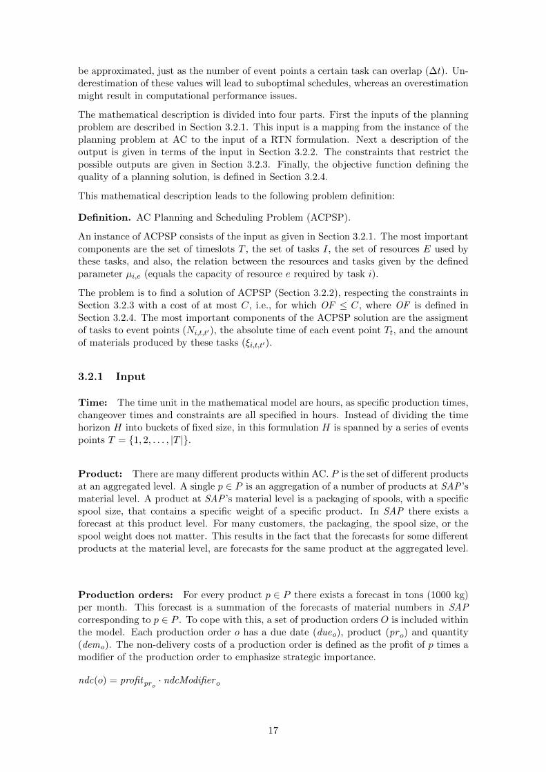
be approximated, just as the number of event points a certain task can overlap (∆t). Un-derestimation of these values will lead to suboptimal schedules, whereas an overestimationmight result in computational performance issues.

The mathematical description is divided into four parts. First the inputs of the planningproblem are described in Section 3.2.1. This input is a mapping from the instance of theplanning problem at AC to the input of a RTN formulation. Next a description of theoutput is given in terms of the input in Section 3.2.2. The constraints that restrict thepossible outputs are given in Section 3.2.3. Finally, the objective function defining thequality of a planning solution, is defined in Section 3.2.4.

This mathematical description leads to the following problem definition:

Definition. AC Planning and Scheduling Problem (ACPSP).

An instance of ACPSP consists of the input as given in Section 3.2.1. The most importantcomponents are the set of timeslots T , the set of tasks I, the set of resources E used bythese tasks, and also, the relation between the resources and tasks given by the definedparameter µi,e (equals the capacity of resource e required by task i).

The problem is to find a solution of ACPSP (Section 3.2.2), respecting the constraints inSection 3.2.3 with a cost of at most C, i.e., for which OF ≤ C, where OF is defined inSection 3.2.4. The most important components of the ACPSP solution are the assigmentof tasks to event points (Ni,t,t′), the absolute time of each event point Tt, and the amountof materials produced by these tasks (ξi,t,t′).

3.2.1 Input

Time: The time unit in the mathematical model are hours, as specific production times,changeover times and constraints are all specified in hours. Instead of dividing the timehorizon H into buckets of fixed size, in this formulation H is spanned by a series of eventspoints T = {1, 2, . . . , |T |}.

Product: There are many different products within AC. P is the set of different productsat an aggregated level. A single p ∈ P is an aggregation of a number of products at SAP ’smaterial level. A product at SAP ’s material level is a packaging of spools, with a specificspool size, that contains a specific weight of a specific product. In SAP there exists aforecast at this product level. For many customers, the packaging, the spool size, or thespool weight does not matter. This results in the fact that the forecasts for some differentproducts at the material level, are forecasts for the same product at the aggregated level.

Production orders: For every product p ∈ P there exists a forecast in tons (1000 kg)per month. This forecast is a summation of the forecasts of material numbers in SAPcorresponding to p ∈ P . To cope with this, a set of production orders O is included withinthe model. Each production order o has a due date (dueo), product (pro) and quantity(demo). The non-delivery costs of a production order is defined as the profit of p times amodifier of the production order to emphasize strategic importance.

ndc(o) = profitpro · ndcModifiero

17

Recipes: R is the set of different product recipes. A single r ∈ R is the recipe to producea single p ∈ P . A single p ∈ P might have more than one recipe r ∈ R.

Resources: There are two different types of resources, primary and secondary resources,involved in producing products p ∈ P . The primary resources are the resources that actu-ally produce the product and the secondary resources are resources that are constrainingthe primary resources with a certain capacity.

• H is the set of high-rise resources. Every h ∈ H has a certain throughput capacity.

• L is the set of production lines. Every production line is linked to one h ∈ H.

• S = {D,E, F,K, P, S,X} is the set of different spinneret types. Each production re-quires a certain type of spinneret and the total number of the same type of spinneretsin use is limited given by capacity spCaps for (s ∈ S)

Changeovers: When recipes r ∈ R and r′ ∈ R are produced in sequence on the sameproduction line, a changeover takes place. The time of the changeover is defined bythe changeover type. There are four different types of changeovers (Section 3.1), eachwith its own length in hours. The parameter ttf r, refers to the type, titer and filamentsidentification of the product produced by recipe r. Other more trivial parameters arefound in the nomenclature section.

For changeovers the following functions exist for r, r′ ∈ R:

• cType(r, r′) ∈ {no, soft, normal, block, spin} are the changeover type between recipesr and r′.

• ct(r, r′) returns the changeover time between recipes r and r′.

Current production: At t = 0, for all production lines l ∈ L there exists a recipe r ∈ Rcurrently being produced at l. This is relevant for the possibly needed changeovers at thestart of the schedule.

Tasks: The set of spinning tasks Ispin consists of all recipes that are possible for eachproduction line subject to all the line/recipe constraints. These constraints are omittedin this version of the document.

Ispin ={(r, l) ∈ R× L | production line l satisfies the classified technical constraints of r}

Next the following set of changeover tasks is defined:

Ico = {i ∈ cType(r, r′)|r, r′ ∈ R} \ {no, soft}

General resources: To keep track of each resource over time all resources are general-ized as specified in equation 3.1. The maximum capacities of these resources are omittedin this version of the document.

E = H ∪ L ∪ S ∪ (other classified technical resources) (3.1)

18

The required capacities for each task i and resource e is defined by µi,e and is as follows:

µi,e =

tpr(i) if i ∈ Ispin ∧ e ∈ H ∧ hrRes l(i) = e,

1 if i ∈ Ispin ∧ e ∈ L ∧ e = l(i),1 if i ∈ Ispin ∧ e ∈ S ∧ e = spinneretr(i)

1 if i ∈ Ico ∧ e ∈ L ∧ e = l(i),0 otherwise.

(3.2)

3.2.2 Output

A solution of the ACPSP consists of an allocation Ni,t,t′ of tasks to event points and theamount of product ξi,t,t′ produced by these tasks. Ni,t,t′ is a binary variable that indicateswhether task i runs from even point t to event point t′. The variable ξi,t,t′ determines theamount of material produced by task i from event point t to t′. The absolute time of eachevent point t ∈ T is given by the variable Tt. Also we have the inventory level of eachproduct p ∈ P given by Ip,t for each t ∈ T . The non-delivered amount of each productionorder o at event point t, is given by the slack variable pslo,t. The binary variable poo,t

decides whether order o is (partially) fulfilled at time t. Notice that each production ordero can only be delivered on at most one event point t ∈ T . An example of the output for3 production lines is given in Figure 3.1. The grey striped tasks represent the changeovertasks. ∆t is set to 4 in the example, so all tasks can maximally overlap 4 intervals.

If a certain task i ∈ I is excuted and Ni,t,t′ = 1, this means that all resources e ∈ E requiredby task i (given by µi,e) should be consumed at event point t and freed at t′. Also theamount of product produced (ξi,t,t′) should correspond to the duration of the interval.Namely, the recipe of task i has a certain throughput and the amount produced is hencederived from the duration of the inverval divided by this throughput. If a production ordero ∈ O is delivered at time t, given by poo,t, the correct amount should be substracted fromthe inventory level Ip,t accordingly, minus the slack (undelivered amount) pslo,t.

For example, consider task i5 in Figure 3.1. This task runs from event point 3 to 6 andhence Ni5,3,6 = 1. Also, this means that ∀i ∈ I | i 6= i5, Ni,3,6 = 0. The latter holdsbecause the resource SB is consumed at t = 3 by task i5 (µi5,SB = 1) and is thereforeunusable by the other tasks. The amount of material produced by task i5 running onproduction line SB corresponds to the variable ξi5,3,6.

Figure 3.1: Example output for 3 production lines

19

3.2.3 Constraints

Timing: Constraints are needed that relate the amount of time passed between eventpoints and the tasks that are executed on them. Constraint 3.3 states that if a certainchangeover task or production task is executed, the duration of the interval is at leastthe changeover duration (cht i) or the needed production time respectively. The latter isdefined by the amount of material produced ξi,t,t′ and the throughput (tons per hour)of the recipe belonging to task i (tphr(i)). The constraint is stated per production linel ∈ L. To check wether production line l is used by a certain task i, µi,l is used (for theproduction line resources l ∈ L, µi,l only takes the value 0 or 1).

∀l ∈ L ∀t, t′ ∈ T | t < t′ ≤ t+ ∆t, t′ ≤ T

Tt′ − Tt ≥∑i∈Ico

(µi,l ·Ni,t,t′ · cht i)|t′=t+1 +∑

i∈Ispin(µi,l · ξi,t,t′

tphr(i)

)(3.3)

∀l ∈ L ∀t, t′ ∈ T | t < t′ ≤ t+ ∆t, t′ ≤ T

Tt′ − Tt ≤H(1−∑i∈Ico

(µi,l ·Ni,t,t′)|t′=t+1 −∑

i∈Ispin(µi,l ·Ni,t,t′))

+∑i∈Ico

(µi,l ·Ni,t,t′ · cht i)|t′=t+1 +∑

i∈Ispin(µi,l · ξi,t,t′

tphr(i)

)(3.4)

Notice that since changeover times are relatively small compared to production times, itis assumed that they can last only one time interval. Moreover, the summations of thechangeovers and the production tasks can be taken together, because only one task can beexecuted at each interval at the same time due to the resource balance constraints. Viceversa, constraint 3.2.3 states that a maximal processing time should be accounted for. Ifno task can be executed between two event points, there should not be an upper boundbetween two event points on the amount of time passed.

Operational: Constraint 3.5 expresses that a minimal amount of material should beproduced (depending on the recipe) if a spinning task is executed. The upper bound isspecified a the maximal amount that can be produced if the whole time horizon was used.Notice that the minimum production time of a recipe of a task (mptr(i)) should be largerthan zero, otherwise Ni,t,t′ can be equal to one (and thus executed), while no material isproduced.

∀t, t′ ∈ T i ∈ Ispin | t < t′ ≤ t+ ∆t, t′ ≤ Tmptr(i) · tphr(i) ·Ni,t,t′ ≤ ξi,t,t′ ≤ H · tphr(i) ·Ni,t,t′

(3.5)

Resource balance: The variable Ee,t maintains the amount of resource e available atevent point t. This amount equals the starting amount (Emax

e |t=1 )plus the amount ofresources that are freed up by all previously executed tasks (those ending at t) and minusthe consumption of all starting tasks (beginning at t). Constraint 3.7 states that theamount of resource can not be empty at each event point. The parameter µi,e specifies

20

the amount of resource e that is required by task i.

∀e ∈ E ∀t ∈ T (3.6)

Ee,t =Emaxe |t=1 + Ee,t−1|t>1 +

∑i∈Ispin

∑t′∈T

t−∆t≥t′<t

µi,e ·Ni,t′,t −∑t′∈T

t<t′≤t+∆t

µi,e ·Ni,t,t′

+∑i∈Ico

µi,e ·Ni,t,t−1

∣∣∣∣∣t>1

−∑i∈Ico

µi,e ·Ni,t,t+1

∣∣∣∣∣t<|T |

∀e ∈ E ∀t ∈ T 0 ≤ Ee,t (3.7)

Inventory: Similar to the resource balance constraints the inventory of each product ismaintained as well at each event point by the variable Ip,t. The initial inventory level forproduct p is defined by the parameter I0

p . In addition, the delivery of all production orderso ∈ O is accounted for. This might not be possible at all times, therefore a slack variablepslo,t is introduced that directly accounts for the unsatisfied demand for production ordero (given by demo) at time t.

∀p ∈ P ∀t ∈ T

Ip,t = I0p |t=1 + Ip,t−1|t>1 +

∑i∈Ispinprr(i)=p

∑t′∈T

t−∆t≥t′<t

ξi,t′,t

− ∑o∈O|pro=p

demo · poo,t + pslo,t (3.8)

∀p ∈ P ∀t ∈ T Ip,t ≥ 0 (3.9)

Production orders: If a production order o is (partially) fulfilled at time t, representedby the binary variable poo,t, the event point should have a ending time before or at thedue date of the order. If the order is not fulfilled at all then there is no restriction on thecorresponding event point.

∀o ∈ O ∀t ∈ T Tt ≤ dueo,t + (1− poo,t) ·H (3.10)

Furthermore if a production order o is not (partially) satisfied, then the sum of the slackvariable pslo,t for all t ∈ T should be zero. This is to prevent that the model misuses theslack variable to boost the inventory level, while no production order is satisfied.

∀o ∈ O ∀t ∈ T 0 ≤ pslo,t ≤ demo · poo,t (3.11)

Finally, at most one time point can be used to satisfy each production order o ∈ O.

∀o ∈ O∑t∈T

poo,t ≤ 1 (3.12)

21

Changeovers: To deal with the various changovers for each production line l ∈ L, allpairs of tasks that require a changeover should execute a changeover task (constraint 3.13).To this end all pairs of recipes r, r′ ∈ R that require a changeover and all ordered eventpoints t1, t2 ∈ T | t1 < t2 are considered. The constraint states that between event pointt1 and event point t2 a changeover task must be executed if there is a task executed thatends on t1 and has recipe r, and there is a task started at t2 that has recipe r′, and finally,between event points t1 and t2 no other task is executed.

∀l ∈ L ∀r, r′ ∈ R ∀t1, t2 ∈ T ∀i ∈ Ico | t1 < t2, i′ = cType(r, r′), i′ /∈ {soft, no}∑t∈T

t1≤t<t2

µi′,l ·Ni′,t,t+1 ≥∑t∈T

t−∆t≤t<t1

∑i∈Ispinr(i)=r

µi,l ·Ni,t,t1 +∑t∈T

t2≤t<t2+∆t

∑i∈Ispinr(i)=r′

µi,l ·Ni,t2,t −

∑t∈T

t1≤t<t2

∑t′∈T

t1<t′<t+∆t

∑i∈Ispin

µi,l ·Ni,t,t′

− 1

(3.13)

Remaining constraints: Some product types may not be produced simultaneously.

∀t ∈ T ∀r, r′ ∈ R | ¬allowSim(r, r′)∑u,u′∈T

u′−u≤∆tu>t−∆tu′≥t+1

∑i∈I|ri=r

Ni,u,u′ +∑

u,u′∈Tu′−u≤∆tu>t−∆tu′≥t+1

∑i∈I|ri=r′

Ni,u,u′ < 2(3.14)

3.2.4 Objectives

The objective function of ACPSP is a combination of four different objectives with differentweights. The best output corresponds to the minimum of this fuction.

OF = wndc ×Ondc + wst ×Ost + wpc ×Opc

• Non-delivery costs: One objective of a solution to ACPSP is to minimize thedifference between the production need and the actual production. This differenceis measured as non-delivery costs, i.e. the money that would have been earned if theproduct was produced. The non-delivered amount for each production order o ∈ Ois equal to the demand of the order demo minus any amount that might have beendeliverd at a (single) time point. This is multiplied by the non-delivery costs of theorder (ndc(o)).

Ondc =∑p∈P

∑o∈O|pro=p

[demo −

∑t∈T

poo,t · demo − pslo,t

]· ndc(o)

22

• Stock target: In order to account for uncertainties in the forecast, AC tries to keepthe stock levels of all the products at a defined target. A ACPSP solution shouldkeep all the stocks above their required target. If the stock is beneath its target, thesolution should be penalized for that. The stock target of a product is defined interms of days of sales corresponding to a certain amount in tons.

Ost =∑p∈P

∑t∈T

stcp ·((stockTargetp − Ip,t) ↑ 0) · stDaysp

stockTargetp

The function Ost corresponds to the sum of the stock deficit costs times the numberof days the stock is below the target, per event point per product. Notice this is anapproximation of the actual stock deficit costs as these costs are now only evaluatedat each event point. It is possible to be more precise by introducing a non linearobjective function (as shown in [3]) that compares the inventory level difference andthe time difference between subsequent event points.

• Production costs: When the complete demand can be fulfilled and all the stocks areabove their required target, the next objective is minimizing the production costs.

Opc =∑

i∈Ispin

∑t∈Tt6=T

∑t′∈T

t<t′≤t+∆t

ξi,t,t′

tphr(i)

· cphr(i)

23

24

Chapter 4

Implementation

A solution for solving the planning and scheduling problem at AC has been proposed by[4]. Due to the large problem complexity and size, a powerful and generic software toolfor planning and scheduling is adapted by means of a custom made plugin. The planningtool used within the process is IBM ILOG Plant PowerOps (PPO) [11]. The advantage ofusing PPO is that an entire framework is already incorporated for solving generic planningand scheduling problems. Namely, several solving methods and algorithms are alreadyincorporated. Some of these methods are discussed in Chapter 2. Another advantage ofusing PPO is that a rich GUI is also already included. This is because several convenientviews exist to inspect or adapt the produced schedules and also to view their quality. Tobe able to make PPO usable for the planning and scheduling problem at AC, one has todefine an instance of PPO’s internally used data model. The initial proposed solution by[4], therefore consists of the following two steps:

1. Define an intermediate model that defines the scheduling problem of AC

2. Write a custom plugin (in the Java language) that maps the intermediate data modelto PPO’s internally used data model

Since the creation of the plugin and the intermediate data model, several changes haveoccurred in the organizational context of AC. Several technical constraints, as listed inSection 3.1, have been added and several constraints that were described in [4] have becomedeprecated and are removed.

Because of the many changes and adaptations, in this chapter both the intermediate datamodel and the mapping to PPO’s internal data model are documented. Furthermore,because the two post processing steps in Chapter 5 work on the level of PPO’s internaldata model, also a simplified data model of PPO is included. Finally, the implementationof the objectives that correspond to the mathematical model are described.

4.1 Intermediate data model

The intermediate data model is not included in this version of the document as it containslots of classified information

25

4.2 PPO’s data model

A simplified version of PPO’s partially used data model is given in Figure 4.1. Someparts of this diagram are constructed by referencing the documentation of PPO. Theclasses shaded with a grey background are used by PPO to represent a solution. Hence,regarding the mapping from the intermediate data model to that of PPO, they can beignored.

The main container of PPO’s data model is IloMSModel which contains resources andrecipes. Resources in PPO have natural numbered capacities and can be shut down atcertain times by relating them to a defined calender. Resources can be connected to setupmatrices through a so-called feature. A setup matrix defines for a given set of states S,the duration of each possible pair (S × S)→ N.

Recipes are the core data structure of PPO. A recipe in PPO consists of several activitiesand each activity can be executed in several modes. An activity can have several setupfeatures and a particular state s ∈ S for each feature. If there exists a mode where aresource is connected to a setup matrix with the same feature as that of the activity,setups are respected between subsequent activities on the same resource. Each modecan use one primary resource and can optionally use several secondary resources. Also amode in PPO can produce several materials and can be tied to either a fixed or variableprocessing time. A variable processing time means that the time needed for productionis proportional to the amount of material produced. Similar to a resource, a mode inPPO can be connected to a calendar as well. For the materials in PPO a demand can bespecified at any given time during the planning horizon.

The solving process of PPO is performed uses the classic decomposition method that issimilar to the ones discussed in Section 2.2.3. First a planning problem is solved usingMIP. To this end, the time horizon of the schedule is divided into buckets of user preferredsizes. Then the planning engine determines which recipes to produce in what quantityfor each time bucket and also allocates them to resources. The latter means that theplanning engine already chooses a mode for each planned recipe and each activity. Aplanned production is an instance of IloMSProductionOrder as shown in Figure 4.1. Afterthe planning phase the created production orders, they are batched by the batching engineusing a heuristic programming method. The planned production orders are inspected andmay be split up into several production orders of the same product respecting the minimumand maximum batch size. Also, for each production order, it is determined which partsof the produced quantity go to the stock or the available customer demands (instancesof IloMSDemand). Finally, the batched production orders are scheduled, by schedulingall activities belonging to the chosen recipe of each production order. Notice that at thispoint the scheduling engine can not change the chosen recipes determined by the planningengine, although it may change the chosen mode of some activities. This is a seriousdrawback as is discussed in Section 5.6. The scheduling engine uses CP for the solvingprocess.

4.3 Mapping

The detailed mapping of the intermediate data model to the PPO model is not includedin this version of the document. The mapping involves the creation of several objects inPPO for the elements in the intermediate data model.

26

IloMSModel

IloMSDemandIloMSMaterial

IloMSMode

IloMSActivity

IloMSResource

IloMSRecipe

0..*

hasRecipes

0..*

hasActivityPrototypes

0..*

hasModes

1

hasPrimaryResource

0..*

hasSecondaryResource

0..*

produces

1 0..*forMaterial

IloMSSetupMatrix

0..*

0..*

hasSetupMatix

0..*

hasResources

IloMSSetupActivity0..1

0..*hasModes

IloMSCalendar

0..1

0..*

hasCalendar

0..1

0..*

hasCalendar

IloMSProductionOrder

0..*

0..*1

IloMSSchedulingSolutionIloMSBatchingSolution

IloMSAbstractActivity

0..*

1curBatchingSol

IloMSScheduledActivitystartTime:int;endTime:int;modeNumber:int;

1curSchedSol

1

0..n

hasScheduledActivities

Figure 4.1: UML diagram of PPO’s internal data model

4.4 Objectives

Currently, the following objectives are implemented:

4.4.1 Inventory deficit costs

The inventory deficit costs is measured by the total surface that a product quantity isbelow the stock target of the product. The objective is implemented according to thecorresponding formula in the mathematical model. The difference is that in PPO theentire surface below the stock target is seen as inventory deficit costs, instead of only atseveral time points as in the mathematical model.

4.4.2 Non-delivery costs

These costs are measured according to the formula specified mathematical model. Anotherimplemented objective is the normalized non-delivery cost. These costs are same, exceptthat the multiplier (ndcModifierp) in the mathematical model and ndcModifier in theintermediate model are set to 1 for each product. This gives better insights in the actualcosts of the produced schedules.

4.4.3 Setup costs

These costs measure the total setup time for all changeovers in the model. This canbe multiplied by a multiplier to emphasize importance of fewer changeovers. Less largechangeovers, namely spinneret changes, lead to more total production. However it mightalso be the case that less demands can be satisfied.

27

28

Chapter 5

Improvements

In this chapter all the improvements and features added to the original model, in com-parison to the version described in [4], are documented. These improvements include arounding error fix of the planning horizon (Section 5.1), a fix in the original mathemat-ical model regarding the inventory deficit costs objective (Section 5.2), simultaneouslyoptimizing the non delivery and the inventory deficit costs (Section 5.3), and finally, aconstraint relaxation regarding the production lines that share a high rise resource (Sec-tion 5.4). This is followed by a final comparison of the original model and the model withall implemented improvements in Section 5.5, showing a significant cost reduction. Noticethat the improvements, as listed in this chapter, only improve the performance of theinitial model. Also, the comparison test results are derived from the same original inputdata and the same technical constraints as that of the initial model.

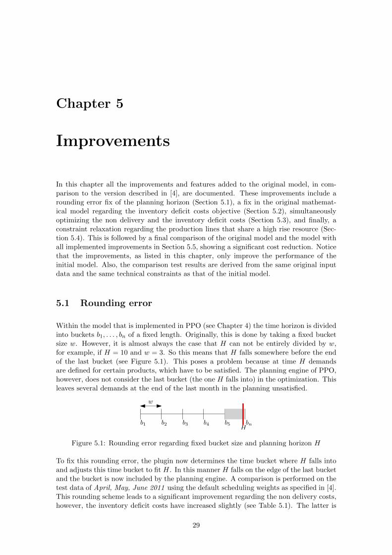
5.1 Rounding error

Within the model that is implemented in PPO (see Chapter 4) the time horizon is dividedinto buckets b1, . . . , bn of a fixed length. Originally, this is done by taking a fixed bucketsize w. However, it is almost always the case that H can not be entirely divided by w,for example, if H = 10 and w = 3. So this means that H falls somewhere before the endof the last bucket (see Figure 5.1). This poses a problem because at time H demandsare defined for certain products, which have to be satisfied. The planning engine of PPO,however, does not consider the last bucket (the one H falls into) in the optimization. Thisleaves several demands at the end of the last month in the planning unsatisfied.

b1 b2 b3 b4 b5 bnH

w

Figure 5.1: Rounding error regarding fixed bucket size and planning horizon H

To fix this rounding error, the plugin now determines the time bucket where H falls intoand adjusts this time bucket to fit H. In this manner H falls on the edge of the last bucketand the bucket is now included by the planning engine. A comparison is performed on thetest data of April, May, June 2011 using the default scheduling weights as specified in [4].This rounding scheme leads to a significant improvement regarding the non delivery costs,however, the inventory deficit costs have increased slightly (see Table 5.1). The latter is

29

likely the case because satisfying demands is more important than satisfying stock targetsaccording to the default planning weights.

non delivery costs inventory deficit costs

original 40.66 385.19

rounding fix 26.10 388.27

Table 5.1: Rounding error cost improvement (millions)

5.2 Inventory deficit cost

In the original mathematical model there is an error regarding the inventory deficit costsobjective. The inventory deficit costs in [4] are specified as follows:

Ost =

∑p∈P

∑0<m≤mmax

stc(p) · 0 ↑ (stockTarget(p)− (0 ↑ st(p,m))

stDays(p)

(5.1)

p is the set of products, m the month within the planning, stockTarget(p) is the amountin ton of p to be in stock, st(p,m) is the actual stock of p in month m and stDays(p) isthe amount of days p should be in stock. Finally, stc(p) specifies the cost per day when pis below the stock target. The objective in equation 5.1 is incorrect because the multiplierstc(p) is specified per day and not per ton. So the amount of days that the stock of pis below the stock target of p should be determined. This can be done correctly by theequation specified as follows.

Ost =

∑p∈P

∑0<m≤mmax

stc(p) · (0 ↑ (stockTarget(p)− st(p,m))) · stDays(p)stockTarget(p)

(5.2)

Fortunately, in the planning tool the inventory deficit costs were implemented accordingto formula 5.2, however, in the planning tool the time units are hours and not days, so thetotal costs should be divided by 24 in the planning tool. This means that all inventorydeficit costs of the earlier results in [4] should be divided by 24 as well. This fact doesnot yield an actual objective improvement, although the relation between the non deliverycosts and the inventory deficit costs changes. Thus, for a fair comparison the model weightshave to be adjusted regarding the changed inventory deficit costs. Another issue is that inthe original model, the inventory deficit costs where also calculated over the extra addedtime buckets beyond the scheduling horizon. This resulted in inventory deficit costs thatwere twice the actual size.

5.3 Simultaneous optimization of non-delivery and inven-tory deficit costs

Within the planning tool, using the original plugin, it is not possible to optimize the nondelivery costs and the inventory deficit costs at the same time in the scheduling engine, asmentioned in Section 6.2 of [4]. To cope with this, in [4] a post processing step is proposedthat explicitly reduces the inventory deficit costs by fixing the production orders for the

30

non delivery costs. The problem regarding the simultaneous optimization appears to resultfrom a constraint regarding the storage capacities. However, since in the model the storageof materials is omitted, this constraint can be left out. Disabling this constraint allowsfor simultaneous optimization of the non-delivery and inventory deficit costs and removesthe need for the mentioned post processing step in the new model.

5.4 Shunt line constraints

One important requirement in the original model, as mentioned in [4], is the following:The polymer concentration for production lines LX and LY can in general maximally differdx and in some rare cases dy. LY is a shunt line of LX, similar to LM and LN.In the planning tool using the original plugin, this problem is tackled by defining a setupmatrix containing all possible polymer concentrations (gathered from all possible produc-tion recipes). A fictional example is given in Table 5.2. By using this method the modelingof the polymer constraint is too strict, because all pair of recipes that differ in polymer cannot be produced simultaneously instead of only the ones that differ in polymer too much.This drawback comes from the fact that the setup matrix has to be fully filled in theplanning tool (each state has to contain a setup to all other states). According to Table5.2, recipes with polymer 0.1 can not be produced together with recipes having polymer0.2 on production lines sharing the same high rise process. However, according to themathematical model, this should be allowed. To cope with this, in the original model, thepossible recipes are copied in the allowed polymer range for all shunt lines. In this mannerthere is always a compatible allowed recipe within the dx range. The scheduling enginehowever has a lot of trouble selecting the right recipes, requiring a necessary manual postprocessing step as explained in Section 6.2 of [4].

polymer 0.1 0.2 0.5

0.1 x x

0.2 x x

0.5 x x

Table 5.2: Example setup matrix, x denotes that two recipes may not be produced simul-taneously

The improved plugin uses a different approach instead of the setup matrix. For each highrise resource that is shared by more than one production line, a resource is created for eachdifferent polymer value . Now the following scheme is applied: One line sharing the highrise resource that produces a recipe seizes all disallowed polymer concentrations, while theother production line requires the actual needed polymer concentration. In the case ofproduction lines LM LN, this would mean that LM seizes all polymer resources that arenot compatible with its current recipe, so that LN is forced to produce a compatible recipe(because that does not require a seized resource). The scheme is the same for productionlines LX and LY only for a different set of polymer resources. Hence the planning engineis forced to plan the right recipes on the shunt lines, as now resources are used to enforcethis behavior. A drawback is that this resource scheme only works when at most twoproduction lines share the same high rise process.

The impact of this improvement is quite extensive since there are two pairs of productionlines that share the same high rise process. The results regarding the costs reduction usingthe default scheduling weights (as specified in [4]) are given in Table 5.3.

31

Performance indicator Original polymer fix

Non-delivery costs 31.2 10.7Inventory deficit costs 15.1 16.8

Table 5.3: Influence of the shunt line constraint improvement

5.5 Evaluation

In this section a comparison is performed between the manual planning solution, theoriginal model from [4], the manual post processing steps by [4] and the model containingall improvement steps as described in this chapter so far. The test is conducted on theinstance of April, May, June 2011. The scheduled downtimes of each resource have beenadded as well. The scheduling weights for the new model are given in Table 5.4, and forthe old model the weights are used as described Section 6 of [4]. Notice, that as explainedin Section 5.2, the inventory deficit cost differ by a factor 24 and this is accounted for inthe new scheduling weights and also in the comparison between all test instances. Also,the scheduling engine now has a weight set for the inventory deficit costs, because thesecosts can be simultaneously optimized.

Performance indicator Planning weight Scheduling weight

Non-delivery costs 2 2Inventory deficit costs 1 1

Setup costs 0 0

Table 5.4: Planning and scheduling weights for the improved model

The results in Table 5.5 and Figure 5.2 show a huge improvement with respect to allcosts in the improved model. Another important fact is that with the latest model thepost processing steps as described in [4] are not required anymore. The setup costs havedecreased slightly in the latest model, while not being part of the optimization. However,the setup costs are still much higher than that of the manual planning solution. Thisconfirms that more changeovers can lead to better costs reductions even though time isneeded for these changeovers. Notice that the results given in Table 5.5 are based onthe old model input data and technical constraints and are only usable for the sake ofcomparison.

Non-delivery costs Inventory deficit costs Setup costs(millions) (millions) (hours)

Manual 38.90 19.42 309Original 26.20 21.86 1289

Original post processed 18.60 21.58 1050Improved 12.01 15.04 956

Table 5.5: Results comparison on test case April, May, June 2011

5.6 Automatic post processing steps

Two automatic post processing steps are added to improve the quality of the resulting so-lutions from PPO. One post processing step reduces the amount of unnecessary spinneret

32

0.00

5.00

10.00

15.00

20.00

25.00

30.00

35.00

40.00

45.00

Manual Original Original post processed Improved

Co

sts

(mill

ion

s)

Non Delivery Cost

Inventory Deficit Cost

Figure 5.2: Results comparison on test case April, May, June 2011

changeovers (Section 5.6.1). Because in PPO a planning problem is solved first, where itis decided what products are produced in which time buckets and also what recipes are tobe used, the scheduling engine can not change these recipes. For the AC scheduling prob-lem this leads to quite a substantial number of unnecessary changeovers per productionline. The second post processing step inflates the scheduled production orders (Section5.6.2). The latter is necessary because the production lines contain many small gaps be-tween the scheduled production orders of PPO. These gaps can often be filled with usefulproductions. The impact of the post processing steps is evaluated in 5.6.3.

5.6.1 Minimizing changeovers

This post processing steps scans for each production line (i.e. the corresponding instancesof IloMSresource), the products to be produced and finds possible alternative recipes forthese products actively minimizing the amount of changeovers. This is illustrated in Figure5.3(a). The nodes in the graph represent the possible recipes for each material (m1 . . .m6)belonging to the production orders. The edges represent the changeover cost to eachsubsequent node. The shortest path in this directed graph represents a set of recipe choices(nodes along the path) that lead to a minimum amount of scheduled changeovers. To findthe shortest path for this special type of graph, a dynamic programming algorithm hasbeen implemented. The implementation of the algorithm is shown in Figure 5.3(b). Afterthe possible alternative recipes are gathered for each material, the algorithm calculatesthe total minimum setup required for each material. The edges in Figure 5.3(b) representthe total minimal setup costs so far. This starts from the leftmost material and ends atthe rightmost material. Next, working backwards, the minimal path is chosen and theproduction orders are adapted accordingly.

After the shortest path is found the scheduled production orders on the production line areassigned the newly chosen recipes. This might result in changeovers that are removed andin some cases a changeover might be introduced. The overall total number of changeovers isminimal however. In the worst case scenario an introduced changeover might be scheduledduring the weekend, as this is difficult to detect by the algorithm. Should this occur,slight manual post processing has to be done to rearrange the allocated changeovers.

33

24

2424

24

24

2424

0 0

24 0

24

00

24 24

m1 m2 m3 m4 m5 m6

(a) Post processing step 1

24

2448

72

96

96

0 0

24 24

48

72

72 96

m1 m2 m3 m4 m5 m6

(b) Post processing step 2

Figure 5.3: Post processing step for a single production line

The removed changeovers lead to gaps that can possible be filled by the subsequent postprocessing step as discussed in the next section. Should filling not be possible (due to forexample a resource constraint) a little manual post processing can be used to fix the smallgap.

5.6.2 Inflating the scheduled production orders

This post processing step inflates the scheduled production orders as much as possible,until either a resource conflict arises or a scheduled downtime is reached. The procedureworks entirely in the data model of PPO and can be applied to production orders of anygeneric PPO problem. The pseudocode of the post processing step is given in Algorithm1.

Algorithm 1 InflateProductionOrders

for po instance of IloMSProductionOrder dominGap← scheduling horizonfor instances of IloMSScheduledActivity ac belonging to po do

mG← scheduling horizonfor instances of IloSMResource r in scheduled mode of ac do

mG← min(mG, size ac can increase without exceeding capacity of r)if r has an upcoming downtime after ac then

mG← min(mG, next downtime of r )end if

end forminGap← min(minGap,mG)

end forincrease production order size to found minGap

end for

5.6.3 Evaluation

To determine the impact of both post processing steps, the instance of April, May, June2011 is evaluated. After PPO has found a scheduling solution, the results are comparedwith and without the post processing steps applied.

The results given in Table 5.6 indicate that inflating the production orders reduces thecosts slightly. However, the inventory deficit cost have increased a little. This can beexplained by an introduced spinneret changeover that removes a day production from acertain production line. Of course more other changeovers are removed, but they might

34

Performance indicator Before After

Non-delivery costs (million) 17.5 17.3Normalized non-delivery costs (million) 10.4 10.3

Inventory deficit costs (million) 6.7 6.8Setup time (hours) 1057 758Spinneret changes 34 19

Table 5.6: Performance impact post processing April, May, June 2011

contribute less (or not at all) towards meeting important stock targets. The removal of aunnecessary spinneret changeover is however always better cost wise.

35

36

Chapter 6

Evaluation

In order to verify and validate the quality of the final model after all model improvements(see Chapter 5), an evaluation study has been conducted. In order to verify that theoutput of the final model is correct and satisfies the technical constraints, a comparisonis made between two manual planning solutions and the corresponding schedules by themodel (Section 6.1). Also, to verify that the model generates solutions that are correctand intuitive, some validation experiments have been conducted in 6.2. Finally, severalwhat-if scenarios and experiments are evaluated in Section 6.3.

6.1 Verification manual planning

In order to compare the model schedules and the manual schedules, two manually designedschedules are created in the model and compared to the output of the model on the sameinput data. The default objective weights used for this verification are given in Table6.1 and correspond to the chosen weights in [4], having the inventory deficit costs weightcorrected (see Section 5.2 of Chapter 5). The time used for the planning engine was 500seconds and the scheduling engine is executed till completion (after about 2500 seconds).The planning engine does not find substantially better solutions after 200 seconds and istherefore capped to 500 seconds.

Performance indicator Planning weight Scheduling weight

Non-delivery costs 2 2Inventory deficit costs 1 1

Setup costs 0 0

Table 6.1: Planning and scheduling weights used for the comparison between the manualand model schedules

6.1.1 Instance April, May, June, 2011

During the creation of the manual schedule in the model, several technical constraints areviolated. The reason is that some of these constraints were not (yet) taken into accountduring the planning process. Furthermore, some constraints turn out to be not so strictin practise. To make a fare comparison between the model and the manually createdschedules some technical constraints have been relieved.

37

Also, the scheduled downtimes and fixed productions present in the manual schedule areadded to the schedule of the model. The summarized results are shown in Table 6.2.There is a large reduction in the top three costs objectives for the model output. Theamount of spinneret changes, setup time, and the total produced amount is worse thanthat of the manual planning though. It should be mentioned some an important factorwas not accounted for in the model.

In the month of April, a very large production order for the product 2040930 A is satisfiedby the model, however a lot less is satisfied by the manual schedule. This is because theforecast of that product has been reduced later and this is adapted afterwards in themanual schedule, but not in the forecast data of that moment. The model hence usesoutdated forecast data. The model result is thus probably of lesser quality, than is shownin Table 6.2 regarding the non-delivery costs objective.

Performance indicator Manual planning Model output

Non-delivery costs (million) 28.9 17.0Normalized non-delivery costs (million) 16.0 10.3

Inventory deficit costs (million) 11.5 6.8Setup time (hours) 350 697Spinneret changes 4 19

Total produced (ton) 5241 4847

Table 6.2: Comparison results April, May, June 2011

6.1.2 Instance Oct, Nov, Dec 2011

Here some constraints are violated as well, during the creation of the manual schedule inthe model.

Also, the scheduled downtimes and fixed productions present in the manual scheduleare added to the schedule of the model. Another important remark is that within thiscomparison no strategically important product have been emphasized. This means thatthe non-delivery costs and normalized non-delivery cost are equal.

Performance indicator Manual planning Model output

Non-delivery costs (million) 5.3 0.1Inventory deficit costs (million) 12.5 7.3

Setup time (hours) 350 975Spinneret changes 8 29

Total produced (tons) 4842 4574

Table 6.3: Comparison results Oct, Nov, Dec 2011

The summarized results are shown in Table 6.3. Interestingly, the non-delivery costs arecloser to each other in comparison to the results of April, May, June, 2011. This mayresult from the fact that there are no forecast data errors like there were in the instanceof April, May, June, 2011. Although the model shows a cost reduction, many moresetup time is used and especially a lot more spinneret changeovers. This large amount ofchangeovers is even present after minimizing the amount of setups per production line bythe first post processing step, as discussed in Section 5.6.1. The reason for this might be

38

the extra constraints that have been added compared to those present in the instance ofApril, May, June 2011.

Notice that also in this case, the model schedules still shows some small gaps. These gapsare mostly at the start of the production lines, because a minimum of 5 days productionis required in the model and the gaps are too short to fill with production. In practice,however, this could be resolved by lengthening the previous running recipes for one or twodays.

6.2 Validation

Some validation experiments are conducted to improve the confidence in the model. Theresults from these experiments are considered as classified information and have beenomitted in this version of the document.

6.3 Analysis

6.3.1 Nondeterminism

A problem with PPO is that it suffers from nondeterminism. This means that differentruns (i.e., solving the same instance multiple times), can lead to different results. Toinvestigate this behavior, a similar problem instance of April, May, June 2011 is solvedmultiple times and the cost outcome is summarized. Because the outcome of each run isindependent, a 95% confidence interval can be constructed using the normal distribution.This only holds if we have sufficient runs.

Run Non-delivery Non-delivery (n.) Inventory deficit Setup

1 12.99 8.49 6.84 745

2 13.34 8.85 6.87 674

3 12.09 8.19 7.41 689

4 12.46 7.90 10.76 859

5 12.34 7.99 10.84 693

6 10.19 7.25 9.02 811

7 13.30 8.80 6.88 683

8 12.11 7.77 10.86 690

9 13.30 8.80 6.90 690

10 13.30 8.80 6.89 683

11 10.55 8.03 8.77 614

12 12.42 7.89 7.21 786

13 11.94 7.55 7.54 675

14 11.50 8.07 7.06 753

15 12.08 8.32 7.00 785

Min 10.19 7.25 6.84 614

Max 13.34 8.85 10.86 859

Avg. 12.26 8.18 8.06 722

Std. Dev. 0.96 0.49 1.58 65.16

95% conf. [11.77;12.75] [7.93;8.43] [7.26;8.85] [689.02;754.98]

Table 6.4: Costs summary of multiple runs of the instance of April, May, June 2011

39

The results (Table 6.4) show a cost summary for the (normalized) non-delivery costs andinventory deficit costs (million euros), and also the setup costs (in hours). This overviewshows that there exists a large variation in the outcome of the same problem instance.This means that when comparing the model solutions of two problem instances, no reliableconclusions can be drawn if only a single run is executed (the outcome of one probleminstance, might be better by coincidence). To fairly evaluate the costs of a single scenario,the average of multiple runs has to be used. The number of runs should be sufficientlylarge as well. Notice that for even 15 runs, the confidence intervals are still fairly large.In order to make reliable predictions when comparing the outcome of the model, at least20 to 30 runs will probably have to be used.

6.3.2 Non-delivery versus inventory deficit costs

One of the improvements, as stated in Chapter 5, is that the non-delivery and inventorydeficit costs can now be simultaneously optimized. Therefore an analysis has been madeto compare the weights used for these costs. To this end the instance of April, May,June 2011 is used. Notice that the since we are now comparing between model results,the scheduled downtimes and fixed productions are not added to the schedules of themodel. Note that it is not useful to investigate scenario’s with higher weights for theinventory deficit costs, since at AC it is always a higher priority to satisfy demands overstock. Furthermore, only one instance is solved for each weight setting. The results ofthe nondeterminism investigation in Section 6.3.1 show that different runs should could beused for each weight setting, to be more accurate. However, the purpose of this experimentis to investigate the impact of the weights rather than giving a true cost prediction.

Weights ObjectivesNon-delivery Inventory deficit Non-delivery Inventory deficit

1 0 7.5 12.94 1 11.7 6.42 1 11.1 7.44 3 11.9 6.71 1 10.3 7.3

Table 6.5: Comparison results Oct, Nov, Dec 2011

The results in Table 6.5 show that there is little variation in the total non-delivery costs,regardless of the used weights. This does no hold if the weight is zero for the inventorydeficit costs. In that case, the non-delivery costs are much lower compared to the othertest results. The weight distribution does however seem affect the inventory deficit costsby a large amount. The best results are achieved when the weight of the non-delivery costsis set not too much higher than that of the inventory deficit costs. Apparently, puttingto much weight on the non-delivery costs, results in the model putting too much effort insatisfying few demands, while it is easier to satisfy the stock targets.

6.3.3 Non-delivery versus setup costs

An analysis has been performed to investigate the influence of these costs on the model,because the costs regarding changeovers of type spinneret are very large for AC. To thisend the setup costs of spinneret changeovers are gradually increased and the impact isobserved on the non-delivery costs. The model is adjusted such that only for spinneret

40

changeovers costs are introduced. The costs of a spinneret changeover is derived in thesame way as was done in [4] by taking the average daily contribution per production lineof 50000 euros per day.

Weights ObjectivesNon-delivery Setup cost Non-delivery nr. of spinneret changes

1 0 11.0 151 1.5 9.4 141 1 13.1 111 2 9.6 111 3 14.2 61 4 8.9 111 6 13.2 71 8 12.1 61 10 12.4 71 15 13.2 101 20 17.3 101 25 26.1 4

Table 6.6: Non-delivery versus setup costs

The results from Table 6.6 indeed show that when the setup costs are gradually increased,the number of spinneret changes are generally reduced in the schedules generated by themodel. This comes at the costs of the non-delivery costs. Notice that these results are stillvery susceptible to PPO’s non-determinism. However, even with the first post processingstep enabled (Section 5.6.1), the model is unable to find the minimal number of setupsthat can be used as the setup costs get very large. Namely, the manual solution shown inSection 6.1, shows that a solution exists that uses just four spinneret changeovers. Thebest solution found by the model (regarding the setups) also uses four changeovers and hascomparable costs, however, visually inspecting the model solution shows many large gapsand even an empty production line. From this we can conclude that the PPO model stillhas issues regarding the setup minimization. This result weakens the initial assumptionthat more changeovers are the necessary result of a better cost reductions. However, notethat this result does not invalidate the assumption that minimizing the amount of setupsdoes not minimize the costs.

41

42

Chapter 7

Conclusion

The goal of this project was to improve the existing planning and scheduling solution forthe production process at AC. The initial proposed solution by [4] showed potential andseveral improvements have been identified since then. One type of improvements involveadaptations made to the data model used by the planning tool. This is achieved by makingadaptations to the mapping from the intermediate data model that is used to contain aproblem instance. To compare the performance of the current model with the originalone by [4], a comparison was made between a manually created schedule and the scheduleoutcomes of both models. The following results have been found:

• The two manual post processing steps needed to improve the quality of the producedschedules of the original model are not required for the new model.

• The non-delivery costs and inventory deficit costs showed a cost reduction of 60%and 20% respectively in the current model. This is against the 17% and even anincrease of inventory deficit costs for the first model. Moreover the setup costs usedby the current model are reduced slightly although not part of the optimization.Note that these results were obtained using the original input data.

• The resulting output of the schedules lead to less gaps and better filling of the heavilyconstrained production lines.

To further boost the model’s performance an automatic post processing step is imple-mented that inflates the production orders of the produced schedules and removes the fewsmall gaps that still existed (if possible). Although this only leads to minor cost reduc-tions, the resulting schedules look more realistic. The new model has been thoroughlytested and the output is reviewed in detail. As a result, some technical constraints havebeen changed and refined in the current model. Also, several large errors in the inputdata have been corrected. These adaptations greatly influenced the models performanceand also increased the quality of the manual plans when put into the model. In order toevaluate the current modeling solution better, a new objective is added to measure thenormalized non-delivery costs.

To evaluate the current model a new comparison is made for two problem instances be-tween the model outcomes and the corresponding manual schedules. The model output ofApril, May, June, 2011 shows a reduction of 41% in non-delivery costs and another 41%in inventory deficit costs. However, a large portion of the difference in non-delivery costshas been explained by outdated forecast data in the models input data. The model resultsof Oct, Nov, Dec 2011 show a schedule with almost no non-delivery costs at all comparedto the manual plan and also a reduction of inventory deficit costs by 42%. This leads to an

43

overall costs difference (non-delivery plus inventory deficit) of 60%. From this perspectivethe model quality is good, however, the setup cost objective suggests there may be roomfor improvement. Also, be aware that not all cost objectives have been implemented yet.

The schedules produced by the model contain more large changeovers (of type spinneret).As suspected by [4], this difference was due to the many more different demands beingsatisfied by the model. However, after more careful inspection, the scheduling engine tendsto generate unnecessary changeovers. Even though another post processing step has beenimplemented to remove all unnecessary changeovers per production line, the schedulingengine still has issues when trying to minimize the amount of setups used. This has beenconfirmed with an experiment in Section 6.3.

Although the current model might be suboptimal regarding the setup time reduction, it isstill of better quality than the manual schedules, i.e., leads to a better objective functionvalue. Also the model can still be used to evaluate several interesting what-if scenarios.Furthermore, as part of the testing, and in order to increase the confidence in the currentmodel, several validation experiments have been performed. To be able to use the currentplanning solution for the comparison between several what-if scenarios however, one hasto be aware of the nondeterministic behavior regarding PPO. This behavior has beeninvestigated with another experiment in Section 6.3.1.

7.1 Future work

As stated in the conclusion, the performance of the current model has thoroughly beenimproved. Also, the model is better comparable to the manual planning. However, thereis still an open issue regarding the minimization of the amount of changeovers. Further-more, due to time constraints and many last minute changes to the model (input dataand constraints), several experiments have not yet been performed. Hence the followingsuggestions are made for future work:

• The current planning and scheduling engine of PPO is suboptimal regarding theminimization of setup costs. An improvement would be to write a custom engine thatcan handle the setup costs better. Given the environment of PPO the best optionwould be to use CP for this. MILP can also be used, however, some constraints andobjective functions might be difficult to linearize.

• Investigate the use of a totally different scheduling solution (outside of PPO). Severalpossibilities have been identified in the literature (Chapter 2). This could be usedas a second verification method along side of the current PPO solution. Optionally,this solution can implement the MILP formulation as discussed in Chapter 3. Anadvantage of using MILP for the entire solving process is that there exist manydeterministic solving algorithms, so that the current nondeterminism problem ofPPO would not be an issue.

• Implement the remaining optimization criteria regarding the transportation costsand also resort allocation.

• Continue to investigate scenarios regarding the configuration of production lines andtechnical constraints. To this end the current solution can be used as a tool. It hasbeen shown that several runs of each scenario have to be compared though, in orderto make reliable predictions.

44

Nomenclature

High rise resources

hrCaph throughput capacity of h in kilos per hour

Production lines

hrRes l high rise resource h used by production line l

minTpl minimum throughput required on l

name l identification of l

Model parameters

∆t maximal number of events points a task can overlap

demo specifies the quantity of production order o

dueo due time of production order o

Emaxe maximum capacity of resource e

cht i changeover time (in hours) needed for changeover task i

µi,e required capacity of resource e by task i

ndcModifiero modifier to enforce strategically important value of production order o

pro specifies the product of production order o

l(i) production line l of task i

r(i) recipe r of task i

H time horizon

I0p initial stock of product p

Objectives

Ondc total non-delivery costs

Opc total production costs

OF total objective outcome

wndc weight of non-delivery costs

wndc weight of stock deficit costs

wpc weight of production costs

Products

45

profitp profit of product p per ton in euros

stcp cost per day of supply when the stock is below the stock target

stDaysp total days of sales p corresponding to stock target

stockTargetp stock target of product p in tons

Recipes

allowSimr,r′ wether if two recipes r, r′ are allowed to be produced concurrently

mptr minimal processing time (in hours) of recipe r

pr r product p produced by recipe r

spinneretr required spinneret for r

spoolweightr spool weight of r

titer r weight (in grams per 10 kilometers) of the product produced by r

tpr throughput required of the high-rise resource for r in kilos per hour

tphr the number of tons produced per hour by r

ttf r type, titer and filaments identification of the product produced by r

typer integer type number of the product produced by r (without the optional “D”in front of it)

Sets/indices

Ico changeover tasks

Ispin spinning tasks

E, e generalized model resources

H,h, h′ high rise resources

I, i, i′ processing tasks

L, l production lines

O, o, o′ production orders

P, p, p′ products

R, r, r′ production recipes

S, s spinneret types

T, t, t′ event points

Variables

poo,t binary variable deciding wether production order o is (partially) fulfilled atevent point t

pslo,t slack (unfulfilled demand) of production order o at event point t

ξi,t,t′ total amount of material processed by task i, starting at t and finishing at t′

Ee,t excess amount of resource e at event point t

Ip,t amount of product p at event point t

46

Ni,t,t′ binary variable that assigns the end of task i, which began at t, to point t′

Tt absolute time of event point t

47

48

Bibliography

[1] Bassett, M. H., Pekny, J. F., and Reklaitis, G. V. Decomposition techniquesfor the solution of large-scale scheduling problems. AIChE Journal 42, 12 (1996),3373–3387.

[2] Bowman, E. H. The schedule-sequencing problem. Operations Research 7, 5 (1959),pp. 621–624.

[3] Castro, P. M., Barbosa-Pvoa, A. P., Matos, H. A., and Novais, A. Q.Simple continuous-time formulation for short-term scheduling of batch and continuousprocesses. Industrial & Engineering Chemistry Research 43, 1 (2004), 105–118.

[4] Coset, R. Modeling and solving the production scheduling problem at ac. Master’sthesis, Technische Universiteit Eindhoven, 2011.

[5] Dogan, M. E., and Grossmann, I. E. A decomposition method for the simultane-ous planning and scheduling of single-stage continuous multiproduct plants. Industrial& Engineering Chemistry Research 45, 1 (2006), 299–315.

[6] Erdirik-Dogan, M., and Grossmann, I. E. Simultaneous planning and schedul-ing of single-stage multi-product continuous plants with parallel lines. Computers &Chemical Engineering 32, 11 (2008), 2664 – 2683. Enterprise-Wide Optimization.

[7] Floudas, C., and Lin, X. Mixed Integer Linear Programming in Process Schedul-ing: Modeling, algorithms, and applications. Annals of Operations Research 139(2005), 131–162. 10.1007/s10479-005-3446-x.

[8] Floudas, C. A., and Lin, X. Continuous-time versus discrete-time approachesfor scheduling of chemical processes: a review. Computers & Chemical Engineering(2004), 2109–2129.

[9] Harjunkoski, I., and Grossmann, I. E. Decomposition techniques for multi-stage scheduling problems using mixed-integer and constraint programming methods.Comp. Chem. Engng 26 (2002), 1533–1552.

[10] Hooker, J. N. An integrated method for planning and scheduling to minimizetardiness, 2006.

[11] IBM. Information about IBM ILOG Plant PowerOps. http://www.ibm.com/

software/integration/sca/plant-powerops/about/.

[12] Janak, S. L., Floudas, C. A., Kallrath, J., and Vormbrock, N. Productionscheduling of a large-scale industrial batch plant. i. short-term and medium-termscheduling. Industrial & Engineering Chemistry Research 45, 25 (2006), 8234–8252.

[13] Kallrath, J. Planning and scheduling in the process industry. OR Spectrum 24(2002), 219–250. 10.1007/s00291-002-0101-7.

49

[14] Kondili, E., Pantelides, C., and Sargent, R. A general algorithm for short-term scheduling of batch operations. Computers & Chemical Engineering 17, 2 (1993),211 – 227. An International Journal of Computer Applications in Chemical Engin-nering.

[15] Li, W. D., and McMahon, C. A. A simulated annealing-based optimizationapproach for integrated process planning and scheduling. Int. J. Comput. Integr.Manuf. 20 (January 2007), 80–95.

[16] Li, Z., and Ierapetritou, M. Process scheduling under uncertainty: Review andchallenges. Computers & Chemical Engineering 32, 4-5 (2008), 715 – 727. Festschriftdevoted to Rex Reklaitis on his 65th Birthday.

[17] Li, Z., and Ierapetritou, M. G. Integrated production planning and schedulingusing a decomposition framework. Chemical Engineering Science 64, 16 (2009), 3585–3597.

[18] Lin, X., Floudas, C. A., Modi, S., and Juhasz, N. M. Continuous-time opti-mization approach for medium-range production scheduling of a multiproduct batchplant. Industrial and Engineering Chemistry Research 41 (2002), 3884–3906.

[19] Liu, Y., and Karimi, I. Scheduling multistage, multiproduct batch plants withnonidentical parallel units and unlimited intermediate storage. Chemical EngineeringScience 62, 6 (2007), 1549 – 1566.

[20] Maravelias, C. T., and Sung, C. Integration of production planning and schedul-ing: Overview, challenges and opportunities. Computers & Chemical Engineering 33,12 (2009), 1919 – 1930. FOCAPO 2008 Selected Papers from the Fifth InternationalConference on Foundations of Computer-Aided Process Operations.

[21] Mendez, C. A., Cerda, J., Grossmann, I. E., Harjunkoski, I., and Fahl, M.State-of-the-art review of optimization methods for short-term scheduling of batchprocesses. Computers & Chemical Engineering 30, 6-7 (2006), 913 – 946.

[22] Omar, M. K., and Teo, S. C. Hierarchical production planning and schedulingin a multi-product, batch process environment. International Journal of ProductionResearch 45, 5 (2007), 1029–1047.

[23] Pantelides, C. Unified frameworks for optimal process planning and scheduling,1994.

[24] QIAN, Y., PAN, M., and HUANG, Y. Modeling and optimization for schedulingof chemical batch processes. Chinese Journal of Chemical Engineering 17, 1 (2009),1 – 7.

[25] Sundaramoorthy, A., and Karimi, I. A simpler better slot-based continuous-time formulation for short-term scheduling in multipurpose batch plants. ChemicalEngineering Science 60, 10 (2005), 2679 – 2702.

[26] Sundaramoorthy, A., and Maravelias, C. T. Simultaneous batching andscheduling in multistage multiproduct processes. Industrial & Engineering Chem-istry Research 47, 5 (2008), 1546–1555.

[27] Wassick, J. M., and Ferrio, J. Extending the resource task network for industrialapplications. Computers & Chemical Engineering 35, 10 (2011), 2124 – 2140.

[28] Wu, D., and Ierapetritou, M. Hierarchical approach for production planningand scheduling under uncertainty, 2007.

50

[29] Zeballos, L. J., Novas, J. M., and Henning, G. P. A CP formulation forscheduling multiproduct multistage batch plants. Computers & Chemical Engineering35, 12 (2011), 2973 – 2989.

[30] Zhang, H., and Gen, M. Effective genetic approach for optimizing advanced plan-ning and scheduling in flexible manufacturing system, 2006.

[31] Zhang, X., and Sargent, R. The optimal operation of mixed production facilities:a general formulation and some approaches for the solution. Computers & ChemicalEngineering 20, 6-7 (1996), 897 – 904. Fifth International Symposium on ProcessSystems Engineering.

51