1

Improving predictability of high ozone episodes through dynamic boundary conditions, emission refresh and chemical data assimilation during the Long Island Sound Tropospheric Ozone Study (LISTOS) field campaign Siqi Ma1,2, Daniel Tong1,3*, Lok Lamsal4,5, Julian Wang6*, Xuelei Zhang3, Youhua Tang3,6, Rick 5 Saylor6, Tianfeng Chai4, Pius Lee6, Patrick Campbell3,6, Barry Baker3,6, Shobha Kondragunta7, Laura Judd8, Timothy A. Berkoff8, Scott J. Janz4, and Ivanka Stajner9 1Department of Atmospheric, Oceanic and Earth Sciences, George Mason University, Fairfax, VA 22030 USA 2National Research Council, hosted by the National Oceanic and Atmospheric Administration Air Resources Lab, College Park, MD 20740 USA 10 3Center for Spatial Information Science and Systems, George Mason University, Fairfax, VA 22030 USA 4Atmospheric Chemistry and Dynamics Laboratory, NASA Goddard Space Flight Center, MD 20771 USA 5Universities Space Research Association, Columbia, MD 21046 USA 6National Oceanic and Atmospheric Administration (NOAA) Air Resources Laboratory, College Park, MD 22030 USA 7NOAA National Environmental Satellite Data and Information Service, College Park, MD 20740 USA 15 8NASA Langley Research Center, Hampton, VA, 23681 USA 9NOAA National Weather Service National Centers for Environmental Prediction, College Park, MD 20740 USA Corresponding authors: Daniel Tong (qtong@gmu.edu); Julian Wang (julian.wang@noaa.gov)

Abstract. Although air quality in the United States improved remarkably in the past decades, ground-level ozone (O3)

rises often in exceedance of the national ambient air quality standard in nonattainment areas, including the Long Island 20 Sound (LIS) and its surrounding areas. Accurate prediction of high ozone episodes is needed to assist government

agencies and the public in mitigating harmful effects of air pollution. In this study, we have developed a suite of potential

forecast improvements, including dynamic boundary conditions, rapid emission refresh and chemical data assimilation,

in a 3 km resolution Community Multi-scale Air Quality (CMAQ) modeling system. The purpose is to evaluate and assess

the effectiveness of these forecasting techniques, individually or in combination, in improving forecast guidance for two 25 major air pollutants: surface O3 and nitrogen dioxide (NO2). Experiments were conducted for a high O3 episode (August

28–29, 2018) during the Long Island Sound Tropospheric Ozone Study (LISTOS) field campaign, which provides

abundant observations for evaluating model performance. The results show that these forecast system updates are useful

in enhancing the capability of this 3 km forecasting model with varying effectiveness for different pollutants. For O3

prediction, the most significant improvement comes from the dynamic boundary conditions derived from the NOAA 30 operational forecast system, National Air Quality Forecast Capability (NAQFC), which increases the correlation

coefficient (R) from 0.81 to 0.93 and reduces the Root Mean Square Error (RMSE) from 14.97 ppbv to 8.22 ppbv,

compared to that with the static boundary conditions (BCs). The NO2 from all high-resolution simulations outperforms

that from the operational 12 km NAQFC simulation, regardless of the BCs used, highlighting the importance of spatially

resolved emission and meteorology inputs for the prediction of short-lived pollutants. The effectiveness of improved 35 initial concentrations through optimal interpolation (OI) is shown to be high in urban areas with high emission density.

The influence of OI adjustment, however, is maintained for a longer period in rural areas where emissions and chemical

transformation make a smaller contribution to the O3 budget than that in high emission areas. Following the assessment

of individual updates, the forecasting system is configured with dynamic boundary conditions, optimal interpolation of

2

initial concentrations, and emission adjustment, to simulate a high ozone episode during the 2018 LISTOS field campaign. 40 The newly developed forecasting system significantly reduces the bias of surface NO2 prediction. When compared with

the NASA Langley GeoCAPE Airborne Simulator (GCAS) vertical column density (VCD), this system is able to

reproduce the NO2 VCD with a higher correlation (0.74), lower normalized mean bias (40%) and normalized mean error

(61%) than NAQFC (0.57, 45% and 76%, respectively). The 3 km system captures magnitude and timing of surface O3

peaks and valleys better. In comparison with LIDAR O3 profile variability of the vertical O3 is captured better by the new 45 system (correlation coefficient of 0.71) than by NAQFC (correlation coefficient of 0.54). Although the experiments are

limited to one pollution episode over the Long Island Sound, this study demonstrates feasible approaches to improve the

predictability of high O3 episodes in contemporary urban environments.

1. Introduction

Exposure to ambient air pollutants has been associated with detrimental health effects, including cardiovascular 50 diseases and premature deaths (Brunekreef and Holgate, 2002; Kim, 2007; Héroux et al., 2015). Recent decades saw

remarkable improvement in the air quality across the United States. From 1990 to 2015, the United States Environmental

Protection Agency (US EPA) estimated that the emissions of nitrogen oxides (NOx), a major pollutant that controls

regional ozone formation, were reduced from 25.2 to 11.5 million t yr -1 (Feng et al., 2020). The downward trends in NOx

emissions have been verified by ground and satellite observations in large cities (Tong et al., 2015) and in the eastern 55 United States (Zhou et al., 2013; Krotkov et al., 2016). Because of the substantial emission reductions, ground-level ozone

concentrations decreased ubiquitously across the US (Hogrefe et al., 2011; Simon et al., 2015; He et al., 2020).

Regardless of the tremendous improvement in air quality, more than one third of the US population still lives in areas

exceeding the National Ambient Air Quality Standards (NAAQS) for ozone (O3) and/or fine particulate matter (PM2.5)

(US EPA, 2020). Many of these ozone nonattainment areas are located along the northeastern Interstate 95 (I-95, Interstate 60 Highway on the East Coast of the United States) corridor where high density of emissions is produced by transportation

and other industrial sources. Surface ozone is formed from photochemical reactions between NOx and volatile organic

compounds (VOCs) (NRC, 1992), and the high emission density of NOx is a major controlling factor for high ozone

events in this region.

As part of the efforts to understand regional O3 pollution, a multi-agency collaborative study of precursor emissions, 65 ground-level O3 formation and transport in the New York City (NYC) metropolitan region and downwind locations, the

Long Island Sound Tropospheric Ozone Study (LISTOS), was launched. Extensive measurements were collected between

June and September 2018 within the NYC metropolitan area and over the Long Island Sound (LIS). Multiple analyses of

the ozone activities during this field campaign have been conducted using numerical models (Baker et al., 2019; Shu et

al., 2019; Berkoff et al., 2019). 70 Air quality forecasts are a critical tool used by environmental and public health agencies to mitigate the detrimental

effects of air pollution (Eder et al., 2010; Oliveri Conti et al., 2017; Tong and Tang, 2018). Accurate prediction of ambient

ozone and its precursors remains challenging due to inherent uncertainties in the model processes (transport, chemistry

and removal), as well as in model inputs such as emissions, initial concentrations (ICs) and boundary conditions (BCs).

Prior studies have also revealed that air quality models face additional challenges in predicting surface O3 concentrations 75

3

at coastal locations or over complex urban areas, including uncertainties in vertical mixing, deposition processes, spatial-

temporal allocation of emissions to the air quality models (Hogrefe et al., 2007; Tong et al., 2006). Therefore, several

modeling techniques have been developed to improve the forecasting skills of these air quality models (Liu et al., 2001;

Tang et al., 2007). Previous studies (Wu et al., 2008; Sandu et al., 2010) suggested employing data assimilation methods

to adjust the initial conditions of a model to reduce model bias. Optimal interpolation (OI) is a simple data assimilation 80 method used to enhance model prediction (Candiani et al., 2013; Tang et al., 2015; Tang et al., 2017). Considering the

modeling sensitivity to BCs, Tang et al. (2009) examined the impact of six different sources of lateral BCs on the CMAQ

(Community Multiscale Air Quality) forecast ability and the results showed that using global model predictions for BCs

was able to improve the correlation coefficients of surface O3 prediction compared to observations. Evaluations of

different databases and configurations for BCs in short-term and long-term simulations also show that dynamic BCs have 85 a positive impact on numerical predictions (Tang et al., 2007; Makar et al., 2010; Henderson et al., 2014; Khan and Kumar,

2019). However, many of these studies use BCs based on global forecasts of a relatively low resolution (e.g., 1.4° × 1.4°

and 2° × 2.5°). Therefore, databases with higher resolution, such as satellite observations or regional forecasting products,

are introduced to construct boundary conditions that were shown to result in a measurable improvement in model

performance (Borge et al., 2010; Pour‐Biazar et al., 2011). Finally, updating emissions from the base year to the specific 90 forecast year has been shown to be an effective approach to reduce the uncertainties of outdated emission inventories to

increase forecasting accuracy (Pan et al., 2014; Tong et al., 2015, 2016).

This study examines to what extent can various modeling techniques improve O3 and NO2 predictions over LIS and

surrounding areas. As the largest metropolitan area in the United States on the Atlantic Ocean coast, this LIS region

represents one of the most challenging places for air quality modeling. The resolution of the present operational 95 forecasting system, National Air Quality Forecast Capability (NAQFC), operated by the National Oceanic and

Atmospheric Administration (NOAA), is at a 12 km horizontal resolution (Davidson et al., 2008). To better resolve fine-

scale processes such as sea breeze and recirculation of air pollutants at coastal sites, a high-resolution (3km) air quality

forecasting system over the LIS region (LIS3km) has been developed using the latest meteorology and air quality models.

Using observations from ground air quality monitors and the LISTOS field campaign, we evaluate the forecasting skills 100 of the high-resolution air quality forecasting system to predict O3 and NO2 over LIS. Specifically, we use three forecast

improvements - dynamic boundary conditions, rapid emission refresh, and chemical data assimilation - to improve the

LIS3km system. The effectiveness of each technique to improve forecasting skill is assessed using the observations from

the LISTOS and the EPA AirNow network (http://airnowapi.org). Descriptions of the modeling system, forecast

improvements, and observation data are presented in Section 2. Assessments of the CMAQ results with and without 105 different forecast system updates are described in Section 3. The application of the new system to predict a high ozone

episode is demonstrated in Section 4A summary of our findings and concluding remarks are provided in Section 5.

4

2. Methodology

2.1 Study design 110

To simulate ozone variability over a complex coastal urban environment, a high-resolution air quality forecasting

system has been developed for LIS and surrounding areas. The forecasting system is comprised of state-of-the-science

weather, emission, and chemical transport models. The model domain covers eastern Pennsylvania, New Jersey, southern

New York, Connecticut and Rhode Island. While this model domain is large enough to capture key physical/chemical

processes within the LIS area, such as sea breeze circulation and photochemistry, the influence of regional transport 115 outside this domain cannot be adequately represented. Therefore, real-time forecasts from the operational NAQFC (Lee

et al., 2017), produced by the NOAA National Weather Service, are used to provide dynamic boundary conditions to

investigate the effect of this model input on forecasting performance. We also explore the effects of emission adjustment

and chemical data assimilation on forecasting performance.

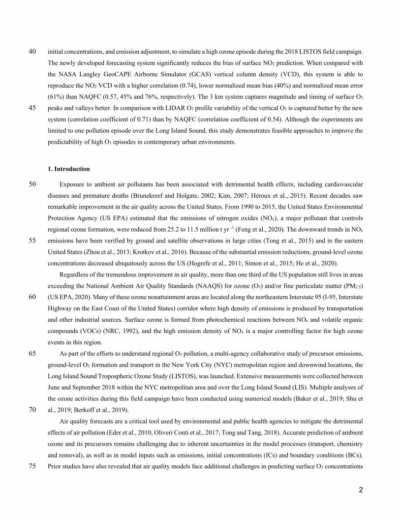
120

Figure 1: Study area over the Long Island Sound and surrounding areas. Red boxes depict four subdomains: New York City (NYC), Philadelphia (PH), New Haven-Hartford region (NHH), and Providence-Pawtucket region (PP). Black circles indicate the locations of EPA ground air quality monitors, the brown triangle indicates the TOLNet O3 site located in Westport, CT, and the blue lines present an example flight path conducted by the NASA B200 aircraft on August 28–29, 2018. Letters a–j 125 indicate surface monitoring sites at: a) Flax Pond, b) Queens College, c) New Haven, d) Westport, e) Colliers Mills, f) Riverhead, g) Greenwich, h) Madison-Beach Road, i) Middletown-CVH-Shed and Stratford.

Five groups of simulations are designed to evaluate the performance and effectiveness of different adjustments of the

CMAQ model (Table 1). The first group (Control run) applies no adjustment, using default profile as LBCs. It serves as 130 the reference case to allow quantifying the effectiveness of each adjustment method. The second experiment, named as

BCON, is similar to the Control run, except that dynamic boundary conditions from the NOAA NAQFC with a horizontal

resolution of 12 km were applied to replace the default BCs. In the Optimal Interpolation (OI) run, the initial

concentrations in CMAQ are adjusted with three observation interpolation methods, including area-average (OI_avg),

inverse distance weighting (idw), and CMAQ concentration gradients (OI_bias) (details of each OI approach provided in 135 Section 2.3(b)). The best performer of these approaches will be used in the subsequent analyses. Next, a group of emission

5

adjustment experiments are designed to update NOx emissions using observed changes from satellite and ground sensors

(Tong et al., 2016). These emission adjustment factors are applied either uniformly across the domain (EmisAdj_whole),

or separately for each subdomain (EmisAdj_sub). In the latter case, the domain was divided into five regions based on

city areas: New York City (NYC), City of Philadelphia (PH), New Haven-Hartford (NHH) and Providence-Pawtucket 140 (PP), and the areas other than these four regions (OTHR) (Fig. 1). Finally, three simulations with the combination of these

three techniques were conducted in search of the best performer. All simulations were conducted for a high ozone episode,

which lasted 168 hours from 0:00 UTC August 25th to 23:00 UTC August 31st, 2018. Table 1. Model adjustment and simulation design for the 3 km forecasting system

Name Description

1 Control Simulation with default profile BCs, no adjustment

2 BCON Same as Control, but BCs replaced with NAQFC prediction

3 OI (3 Cases)

Same as Control, but initial concentrations adjusted by three OI methods (OI_avg, OI_idw and OI_bias)

4 EmisAdj (2 Cases)

Same as Control, but NOx emissions adjusted using observed trends from ground and satellite sensors (EmisAdj_avg, EmisAdj_sub)

5 Combined (3 Cases)

Combination of different techniques. BCON+OI, BCON+OI+EmisAdj_avg, and BCON+OI+EmisAdj_sub

145

2.2 High-resolution air quality forecasting system (LIS3km) The high-resolution air quality forecasting system used here is a new research prediction system deployed during the

2018 LISTOS field campaign period which is comprised of three major components: meteorology, emission, and

chemical transport models. The Weather Research and Forecasting (WRF) model version 4.0 (Skamarock et al., 2019) is

used to generate hourly meteorological fields to drive emission and air quality modeling. The WRF model was configured 150 with Thompson graupel microphysics scheme, RRTMG long and short-wave radiation scheme, Mellor-Yamada-Janjic

PBL scheme, unified Noah land-surface model and Tiedtke cumulus parameterization option. No data assimilation was

applied in the WRF simulation. The model is conducted in a single domain with 132×122 grid cells with one grid more

on each boundary compared to that of the chemical transport model. There are 41 vertical layers with 20 layers below 1

km and top layer at 50 hPa. The forecast fields of Global Forecast System (GFS) version 4 products with a horizontal 155 resolution of 0.25° × 0.25° (available every 6 h) were employed to drive the WRF model.

The emission input was provided using a hybrid emission modeling system that utilized the Sparse Matrix Operator

Kernel Emissions (SMOKE) model (Houyoux et al., 2000) version 4.7 to process anthropogenic emissions, and a suite

of emission models to estimate emissions from intermittent and/or meteorology-dependent sources. Anthropogenic

emissions from area and mobile sources were taken from US EPA 2011 NEI version 2 (NEI2011v2). The Motor Vehicle 160 Emissions Simulator (MOVES) was used to generate county-level emission factors for the onroad and offroad sources.

SMOKE uses a combination of vehicle activity data, MOVES emission factors, meteorology and other ancillary data

(spatial, temporal and speciation information) to generate hourly speciated model-ready emission data. Point sources were

6

processed in two steps. In the first step, emission inventories of point sources were processed with SMOKE to generate

intermediate input files. Next, these intermediate files were used to drive inline calculation of plume rise to distribute 165 point source emissions vertically in the CMAQ model domain. Two natural sources are included in this forecasting system:

biogenic and sea-salt. Biogenic emissions from terrestrial plants were predicted using the inline version of the Biogenic

Emission Inventory System (BEIS) (Pierce et al., 1998). The emissions of sea spray aerosols are calculated using an

updated version of the Gong (2003) sea-spray emission parameterization (Gantt et al., 2015).

The CMAQ model ingests emissions and meteorology to predict spatial and temporal variations of O3, NO2, and their 170 precursors. In this study, version 5.3.1 of the CMAQ model was configured to include detailed implementation of inline

emission processes for biogenic, sea-salt and elevated anthropogenic emissions, horizontal and vertical advection,

turbulent diffusion, dry/wet deposition and full gas, aqueous and aerosol chemistry using a revised Carbon Bond 6 gas-

phase mechanism and AE6 aerosol mechanism (CB6r3_AE6_AQ) (Byun and Schere, 2006; Luecken et al., 2019). Both

the meteorological and air quality models have a 3 km horizontal resolution over the LIS region and its surrounding areas 175 (Figure 1).

2.3 Techniques to improve forecasting skills

We implement and test three forecasting improvement techniques to assess their effectiveness in enhancing the

simulation performance of the CMAQ model. Details of each update are described below.

a) Dynamic lateral boundary conditions 180 Regional air quality models such as CMAQ rely on lateral boundary conditions to account for inflow of air pollutants

and precursors from out-of-domain sources. These boundary conditions fall into two categories: static and dynamic. Static

boundary conditions are time-independent vertical profiles of appropriate species at the boundaries that can be prepared

from prescribed profiles, long-term vertical observations, or climatological model simulations (Tong and Mauzerall, 2006;

Tang et al., 2007). Dynamical boundary conditions are provided by a concurrently running global model or another 185 regional model covering a larger domain. In the previous studies of regional modeling, a nested grid approach was often

applied to provide dynamic BCs for the study area (e.g., Taghavi et al., 2004). However, the nested model would need

higher computational resources and a longer running time. The increasing pool of real-time national and global forecasts

provides alternative BCs that can be used to drive a regional forecasting system as demonstrated in this work. Here, we

explore the feasibility of utilizing the products of NOAA NAQFC, which provides real-time national forecasts to prepare 190 dynamic boundary conditions to drive the LIS3km system. The NAQFC is an operational system, operated by the National

Weather Services, and the data are provided freely to the public. Hourly forecasts of the NAQFC (Lee et al., 2017) are

processed using the BCON tool developed by the US EPA. The description of NAQFC configuration can be found in Lee

et al., (2017) and a summary is provided in Table S1.

b) Optimal Interpolation 195 Optimal Interpolation (OI) is a commonly applied data assimilation method (Wang et al., 2013; Chai et al., 2017) that

can be used to adjust the initial conditions (ICs) of an air quality model to minimize errors (Adhikary, 2008). This method

runs fast and portably, making it very suitable for the forecasting system which needs regular execution. The equation of

the OI method is defined as:

7

𝑥! = 𝑥" + 𝐵𝐻#(𝐻𝐵𝐻# + 𝑂)$%(𝑦 − 𝐻𝑥") (1) 200 where xa and xb are the analyzed and background fields, respectively. B and O are the background and observation error

covariance matrix, H is the observational operator and HT is its matrix transpose, and y is the observation vector.

In the CMAQ model, the restart file, called CGRID, is daily generated during the simulation and acts as ICs for the

next day. To constrain the biases in ICs, the concentrations of ozone, NO2 and NO in the restart file were adjusted via the

OI method, which is applied every 24 hours at 0:00 Coordinated Universal Time (UTC). The influence area of OI is 205 controlled by the correlation length scale and the previous study by Chai et al. (2017) chose the range of 84 km for the

contiguous US domain. Moreover, this influence length scale also varies from region to region. Over remote regions, the

length scale may be longer while it is shorter over polluted areas as the correlation decreases more rapidly. Considering

the high emission density and the fine model resolution over the LIS area, we chose a shorter influence length (33km) for

a higher correlation threshold (r >= 0.5) for the LIS which means this OI adjustment was made on each 11×11 grid cell 210 block of the surface layer over the whole domain to obtain the analyzed field xa. Next, as there is no information of vertical

background profile in this method, the ratio between xa and xb at each surface layer grid point was used to scale the

concentrations for all vertical layers within the PBL, following Tang et al. (2015; 2017).

The OI assimilation first allocates ground-based observational data from the EPA AIRNow network into model grid

cells. The Tang et al. (2015) method puts in-situ data directly into the corresponding model grid cells. If there was more 215 than one active site in the same grid cell, the observations are first averaged before being applied to the grid cell (OI_avg

hereafter). Grid cells that did not have observations and were not within 5 grids cells from the observations were not

adjusted. Therefore, the region of influence is limited, and the adjusted fields may be discrete in spatial distribution.

Besides this method, experiments were also performed with two different interpolation methods for preparing the

observational data. The first one was to interpolate the averaged observational grid points to the whole domain using the 220 Inverse Distance Weighting (IDW) interpolation scheme (Shepard, 1968), (the OI_idw method). With this interpolation,

the effect of OI will be not limited near the observational sites and most of the grid cells in the domain can be adjusted

comparing to the OI_avg. The second method adjusted the initial concentrations by subtracting the bias between the

simulation and the averaged observations within the grid point, then smoothing the adjusted concentration field via the

IDW scheme. This method is called OI_bias. Unlike the OI_idw which just applied the spatial interpolation to extend the 225 OI effect, in this method the observation cells are distributed to the whole domain grids based on the spatial patterns

provided by the model so that it is able to better reflect the realistic fields.

c) Emission refresh

The third forecast system update evaluated here is the rapid emission refresh capability that allows timely updates of

outdated NEIs to the forecasting year (Tong et al., 2016). Here we focus on updating NOx emissions. NOx are important 230 precursors to tropospheric ozone formation (Spicer, 1983; Chameides et al., 1992), therefore, their emissions can

influence atmospheric ozone concentrations. Since NOx emissions decreased substantially over the last decade (Silvern

et al., 2019; Dix et al., 2020) and the anthropogenic emission used in this study are based on the 2011 NEIs, the NOx

emissions need to be projected from 2011 to the forecast year (2018). According to the approach proposed by Tong et al.

(2016), the adjustment factor used for the emission projection is derived from the monthly changing rates of surface- and 235 satellite-observed NOx (NO2). Temporal trends at the surface are determined from the hourly observed NOx concentration

8

during the morning rush hours (06, 07, 08, and 09 local time). These times are optimal for assessing local emission

conditions since they are related to the highest NOx levels typically produced as a result of both commuter traffic peaks

and the shallow morning planetary boundary layer (Tong et al. 2015). Satellite-based temporal trends are calculated from

the monthly NO2 product retrieved from the Ozone Monitoring Instrument (OMI) aboard the Aura satellite (Lamsal et al., 240 2020). A weighting function is introduced to combine the surface-based and satellite-based temporal trends to acquire the

merged projection adjustment factor (AF) for a specified region:

𝐴𝐹 = ∆'×)!×*"+∆,×)#×*#)!×*"+)#×*#

(2)

where ΔS and NS are the temporal trend and the number of satellite data, respectively; and ΔG and NG are the temporal

trend and the number of surface-based data, respectively. Two weighting factors, fS and fG are applied to the satellite and 245 surface data, respectively. Here the value of fS is set to 1 and fG to 100 to avoid dominance by either data source (Tong et

al., 2015). In this study, two groups of AFs are prepared for the emission projection. One is the average AF over the whole

domain (EmisAdj_avg) and the other group includes the AFs for each sub-region in the research area (EmisAdj_sub).

The AFs used in both groups are the averages of the monthly AFs from May to September.

2.4 Observational data sets 250

In this study, a suite of observational datasets was used either as inputs for emissions and chemical data assimilation

or to evaluate model performance. These datasets include surface O3 and NO2 measurements from the US EPA Air Quality

System (AQS) surface network, the NO2 vertical column density (VCD) from the OMI satellite data, NO2 VCD from the

GeoCAPE Airborne Simulator (GCAS) on the NASA Langley Research Center B200 aircraft, and the O3 vertical profile

from the NASA Langley Mobile Ozone Lidar (LMOL). Detailed information of each data set is provided below. 255 Surface concentrations of O3 and NO2 are used for emission adjustment and chemical data assimilation, as well as

evaluation of model performance. AQS is a routine monitoring network established to collect ambient air pollution data

in urban, suburban, and rural areas. AQS monitors determine O3 concentrations according to the Federal Reference

Method promulgated in the 2015 revisions to the National Ambient Air Quality Standards (Long et al., 2014) and NOx

concentrations using the chemiluminescence instruments described by McClenny et al. (2002). AQS measures both O3 260 and NO2 at hourly intervals. Note that NO2 measurements are typically biased high due to interference in the

chemiluminescence measurement (Dunlea et al., 2007). As the goal of this study is to improve forecasting performance,

a near-real-time version of the AQS data was used, called AirNow. This is a preliminary dataset for the purpose of real-

time air quality reporting and forecasting; it is not fully verified and provides fewer measured species. The data used in

this study are downloaded from the AirNow data portal maintained by the US EPA. 265 NO2 VCD measurements were provided by the Ozone Monitoring Instrument (OMI) standard product (version 4),

available from the NASA Goddard Earth Sciences Data and Information Services Center (GES DISC). OMI is a nadir-

viewing hyperspectral imaging spectrometer that measures solar backscattered radiance and solar irradiance in the

ultraviolet and visible regions (270–500 nm) (Levelt et al., 2006). The Aura spacecraft has a local equator-crossing time

of 13:45 h in the ascending node. OMI views the Earth along the satellite track with a swath of 3600 km on the surface 270 in order to provide daily global coverage. In the normal global operational mode, the OMI ground pixel at nadir is

approximately 13 km × 24 km, with increasing pixel sizes toward the edges of the orbital swaths. Multi-year OMI NO2

9

data are further aggregated to calculate state-level emission adjustment factors using a mass conservation approach (Tong

et al., 2015).

The high-resolution NO2 observations from the GCAS (Kowalewski and Janz, 2014) are used for a direct comparison 275 against model simulations of the NO2 VCD. GCAS is an ultraviolet-visible spectrometer used in air quality field studies

to map the spatiotemporal distribution of NO2 and HCHO VCDs at high spatial resolution (Nowlan et al., 2018; Judd et

al., 2020). During LISTOS, this instrument flew on 11 flight days collecting between 2-4 gapless raster datasets at spatial

resolutions for NO2 as fine as 250 × 250 m. More information about the retrieval can be found in Judd et al. (2020).

During LISTOS, NO2 from GCAS was validated using coincident Pandora measurements and had a median percent 280 difference of -1.2% with 95% of the most temporally homogeneous points within ± 25% or 0.1 DU.

Finally, O3 vertical profiles from the NASA LMOL are used to evaluate the CMAQ prediction of O3 profiles during

the LISTOS field campaign. LMOL is part of a NASA-sponsored ozone lidar network called the tropospheric ozone lidar

network (TOLNet; Sullivan et al., 2017), which is a mobile ground-based ozone lidar platform equipped with a pulsed

UV laser and all associated power and lidar control support units (De Young et al., 2017; Gronoff et al., 2019). In this 285 study, we use LMOL lidar observations at the Westport site (41.118° N, 73.337° W). All available field measurement

data during this campaign were obtained from the LISTOS Data Archive (https://www-

air.larc.nasa.gov/missions/listos/index.html).

3. Evaluation on the effectiveness of simulation improvements

3.1 Effects of boundary conditions 290

In this section, we examine the effects of using the dynamic boundary conditions on O3 and NO2 predictions. As a

reference, we also compare these simulations to the NAQFC results, extracted for the same region, during the August 29

high ozone event. Figure 2 shows the O3 and NO2 24-hour average concentrations simulated by Control (static BCs),

BCON (dynamic BCs) and the NOAA NAQFC over the LIS region. Comparing to the underestimated O3 concentrations

simulated by Control run, the concentration level using dynamic boundary conditions increases considerably and is closer 295 to the observations. High O3 concentrations appear over near-coast areas, but are lower in the northwest of the domain.

This spatial pattern illustrates the ozone river in a northeastward direction along the I-95 corridor, extending from

Philadelphia to NYC, and then to Connecticut where the worst air quality is often observed. Although it overestimates

surface O3 in Philadelphia and central New Jersey, the BCON simulation can reproduce O3 hourly variations during this

episode well in comparison with the observed data (see the time series in Figure 2d). Note the peak O3 simulated in the 300 Control run is nearly the same on all days during the simulation period. The comparisons between the peak O3 with the

default profile and dynamic LBC case indicates relatively large regional contributions on these days. Compared to the

Control run, the BCON run performed better not only in bias, but also with higher correlation coefficients between

prediction and observations (Table S2), especially during the August 26–27 high O3 days. As the profile BCs are static

and lack spatial-temporal variations, the Control run mainly reflects the local contributions of emissions, transport and 305 chemical processes within the domain (Tang et al., 2007). The underprediction suggests that these processes are

insufficient to produce the observed O3 levels, and that the transport of air pollutants from upwind is important to predict

10

the high O3 episodes. It highlights the significant influence of dynamic BCs on the simulations over this region during

high pollution events. In comparison, the influence of BCs is less important during the cold season. There is a smaller

difference between upwind concentrations and the background concentrations used in the default BCs, compared to that 310 during a hot season when the upwind photochemical production is more active, resulting in better agreement between the

prediction and observations (Fig. S2a, d). Note that other studies have shown the influence of BCs can become more

prominent during the cold season when “local” pollution production is slow (e.g., Fiore et al., 2009). The magnitude of

the actual influence is determined by several factors, such as emission density, photochemical production and sink, and

spatial distribution and gradients of the concerned species. 315

Figure 2: Predicted O3 concentrations from (a) Control, (b) BCON and (c) NOAA NAQFC simulations on August 29, 2018, and (d) comparison of domain-averaged hourly O3 concentrations with EPA AirNow measurements during this episode. Colored circles at the top panels depict the observed concentrations from ground measurements. 320

The performance of the high-resolution simulation is next compared to that by the NAQFC. The NAQFC simulation,

which has been used to provide national numerical guidance for O3 and PM2.5 (Lee et al., 2017), is run at a coarser

resolution (12 km), using a different CMAQ version (a revised CMAQ5.0), driven by different emission and meteorology

datasets. Regardless of these differences, the NAQFC and BCON runs predict similar surface O3 distribution patterns.

Compared to that in the NAQFC prediction, the O3 prediction from the 3 km BCON run demonstrates more detailed 325 spatial distribution. For instance, the O3 concentration over the Long Island Sound is lower than its surrounding areas

during this episode, which is better resolved by the 3 km simulation than the 12 km NAQFC (Figure 2a-c). The O3

distribution along the coastal area, such as the coasts of Connecticut and Rhode Island, also agrees better with the

observations than the 12 km NAQFC prediction. This suggests that the high-resolution simulation can better reproduce

the pollutant variability over this coastal urban area during this episode. In addition, the BCON run performs better over 330 southern New Jersey, and northeast of the LIS domain, with considerably reduced biases in the LIS downwind areas as

11

well. As to the diurnal variations, the BCON run overestimates the peak O3 concentrations on August 28 and 29, while

the NAQFC run performs well and is closer to the measurements (Fig. 2d). The use of coarser resolution NAQFC

predictions as BCs substantially improves the capability of the 3 km forecasting system to reproduce the O3 variability.

Compared to the Control run, the correlation coefficient between BCON and observed O3 concentrations increases from 335 0.81 to 0.93 and the relative mean square error (RMSE) decreases from 14.97 ppbv to 8.22 ppbv with a reduction of 45%,

resulting in a comparable performance with the NOAA NAQFC predictions with correlation of 0.91(Table S2).

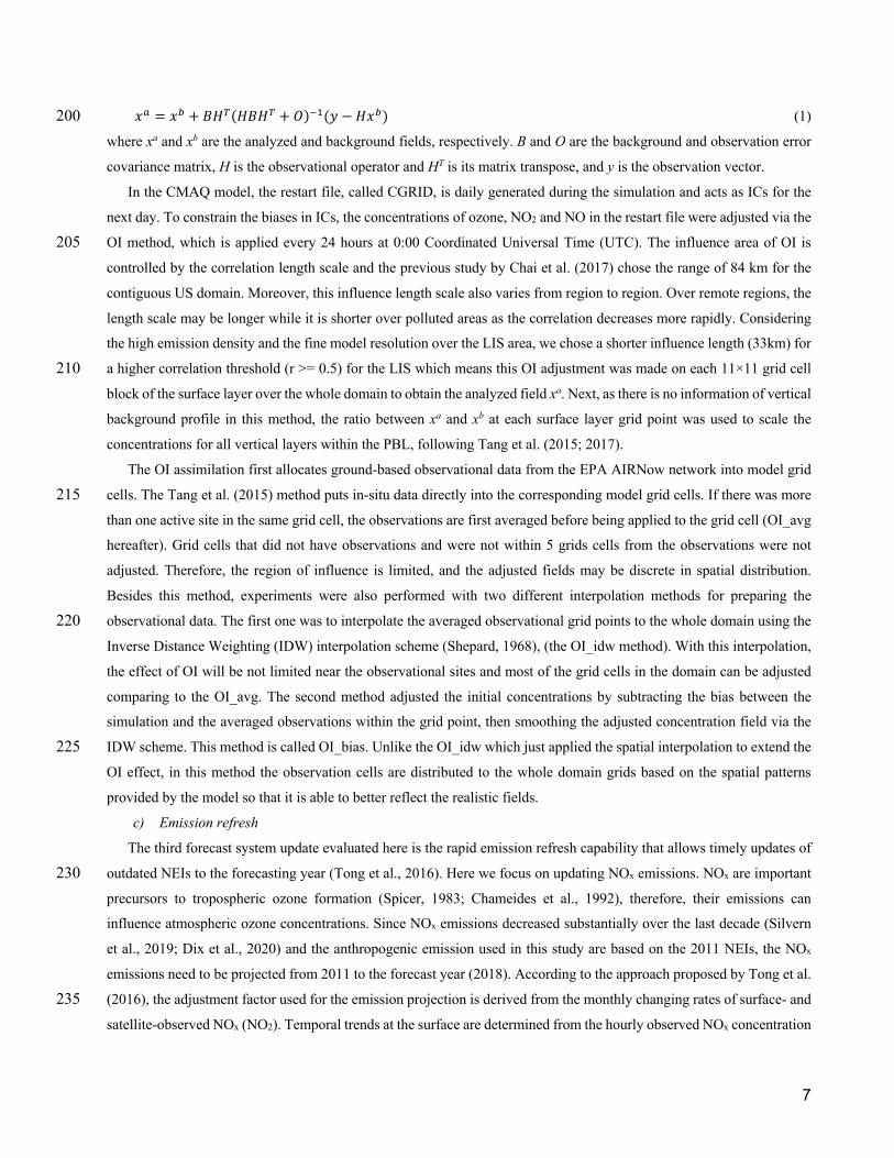
The spatial patterns of predicted NO2 concentrations from the Control, BCON, and NAQFC runs are quite similar

with high values over the NYC area (Fig. 3). The simulated NO2 concentrations by the 3 km forecasting system, either

with static or with dynamic BCs, agree better with the observations than those from the 12 km NAQFC simulation, 340 highlighting the importance of using high resolution inputs to better represent the emission sources in the model. The

correlation coefficient and RMSEs are 0.69 and 4.12 ppb for the Control run, 0.71 and 3.82 ppb for the BCON run, and

0.67 and 4.98 ppb for the NAQFC run, respectively (Table S2). In addition, the improvement of simulated NO2 using

dynamic BCs was much smaller compared to that of O3. This is because the lifetime of NO2 is relatively short (1–7 h in

summertime, Lu et al., 2015), and its budget in urban areas is mainly influenced by local emissions and chemistry, and 345 less by regional transport, indicating the effectiveness of dynamic BCs depends not only on the downwind/upwind

gradients, but also on the lifetime of concerned species.

Figure 3: Predicted NO2 concentrations from (a) Control, (b) BCON and (c) NOAA NAQFC simulations on August 29, 2018, 350 and (d) comparison of domain-averaged hourly NO2 concentrations to EPA AirNow measurements during the episode. Colored circles at the top panels depict the observed concentrations from ground measurements.

12

3.2 Effects of initial condition adjustment

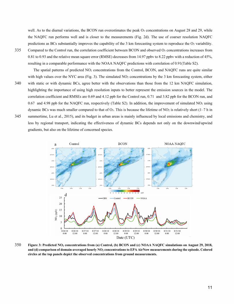
Initial concentrations are an important input to air quality forecasting. Adjusting initial concentrations through 355 chemical data assimilation has been shown to significantly improve air quality forecasting (Tang et al., 2015; Chai et al.,

2017) although the impacts wane with increasing forecast length. Here we compare the results using various OI methods

with the simulations without any BC adjustment (same as the Control run) and study the effects of adjusting initial

conditions on O3 and NO2 prediction. Figure 4 illustrates the initial concentrations of surface O3 adjusted by OI_avg,

OI_idw and OI_bias, respectively. In the initial concentrations, the areas influenced by OI_avg are primarily limited to 360 the ground-based sites and the regions within five model grid cells in each direction of the observations compared to the

Control run (Fig. 4a, b). The rest of the domain is not affected by the adjustment, resulting in significant differences

between adjusted and unadjusted areas. The O3 fields adjusted by OI_idw (Fig. 4c) and OI_bias (Fig. 4d) show similar

horizontal distributions, but the concentration level of OI_bias is relatively higher over NYC and northern New Jersey.

Furthermore, in contrast to the localized changes by OI_avg, those of OI_idw and OI_bias show smoother changes over 365 larger parts of the domain.

Figure 4: The concentrations of surface O3 in initial conditions file at 00 UTC August 26, 2018 adjusted by OI_avg, OI_idw 370 and OI_bias.

Next, the initial concentrations files after adjustment are used to feed CMAQ simulations. The O3 prediction by the

Control run and three OI runs at 00:00 UTC on August 26, 2018 (the first hour after OI adjusting) are depicted in Figure

5. The adjusted O3 fields show different patterns compared to that in the Control run with no IC adjustment. The predicted 375 O3 field with the OI_avg method shows a distribution with localized high value areas near the observational sites. As for

the other two OI methods, the distribution using OI_bias has similar patterns with that of OI_idw while the concentrations

13

over the high O3 area are further elevated. Biases between observed and predicted concentrations are reduced in most

areas. The statistical metrics calculated from hourly simulated and observed data from August 26 to 31, 2018 are reported

in Table 2. The RMSEs for O3 are reduced from 14.97 ppbv in the Control run to 13.72 ppbv in the OI_bias run, to 13.79 380 ppbv in the OI_idw run, and to 14.30 ppbv in the OI_avg run. The correlation for O3 also slightly increases from the

Control run to the OI runs (Table 2). In comparison, NO2 prediction is less influenced by this adjustment, with

insignificant changes in the model performance (Table 3). In addition, the effects of this adjustment on the modeling

results decrease with the simulation time and display no discernible difference from the Control run after 12 hours (Fig.

S1). Generally, the improvement of the simulated results due to OI data assimilation over the study domain is smaller 385 than that from the dynamic BCs. Among the three OI methods, the simulation with OI_bias shows the best performance,

so this method is chosen for subsequent analyses in which multiple techniques are combined to improve forecasting skills.

Figure 5: Spatial distributions of predicted surface O3 concentrations using three Optimal Interpolation (OI) approaches 390 (OI_avg, OI_idw, and OI_bias) at 00 UTC on August 26, 2018.

Table 2: Regional mean statistical metrics between hourly observed and simulated O3 from August 26 to 31, 2018 over the Long Island Sound region

Stats\Runs Control OI_avg OI_idw OI_bias

CORR 0.81 0.84 0.85 0.85

RMSE 14.97 14.30 13.79 13.72

NMB -30% -29% -27% -27%

14

NME 34% 33% 31% 31%

CORR: correlation coefficient, RMSE: relative mean square error, NMB: normalized mean bias, NME: normalized mean error. 395 Table 3: Same with Table 2 but for NO2

Stats\Runs Control OI_avg OI_idw OI_bias

CORR 0.69 0.69 0.69 0.70

RMSE 4.12 4.11 4.08 4.08

NMB -17% -17% -15% -17%

NME 35% 35% 35% 34%

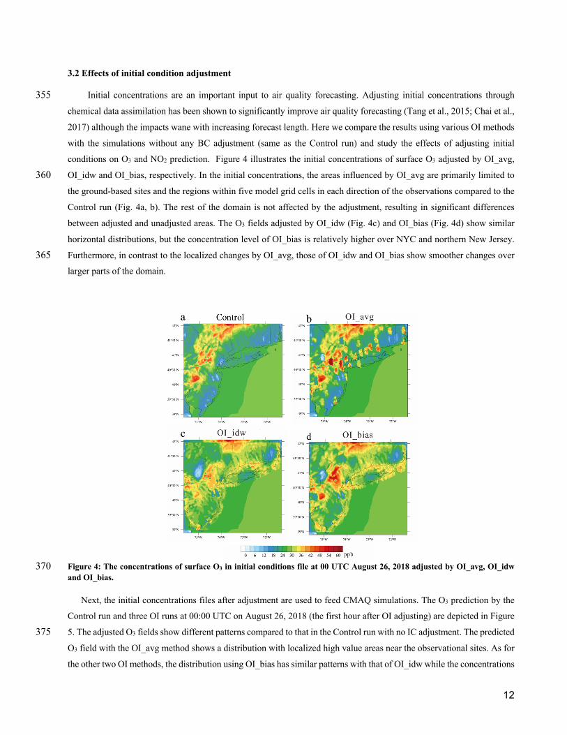
The ICs for each day were adjusted by OI using real time observations, it is interesting to note that the duration of OI

influence on O3 simulation varies from place to place. Figure 6 shows the time series of the averaged differences in 400 predicted hourly O3 concentrations between the Control run and each of the three OI runs from August 26 to 31, 2018 in

three urban areas (NYC, Philadelphia, New Haven – Hartford) and other (OTHR) areas. The differences illustrate the

effect of adjusting initial concentrations on O3 prediction. In large metropolitan areas, OI adjustments result in spikes that

indicate larger model errors at the time of OI adjustment, with the mean errors up to 14 ppbv in surface hourly O3

concentrations over NYC and 16 ppbv over Philadelphia, respectively. In comparison, the spikes in non-urban areas are 405 much smaller, reflecting the fact that there are smaller biases between observations and predictions (Fig. 6). The New

Haven–Hartford region sees a smaller change of O3 concentration compared to between that in large cities. The OI effects

in large cities remain for a shorter time than in non-urban area or smaller cities. For example, the differences between OI

runs and the Control run decrease to ~0 ppb in four to eight hours in two metropolitan areas, NYC and Philadelphia (Fig.

6a, b). Meanwhile, in the New Haven – Hartford region (Fig. 6c), Providence-Pawtucket region (not shown) and the non-410 urban areas (Fig. 6d), the differences could last 12 to 16 hours. The different durations indicate the influence time of OI

adjusted ICs, not necessarily the improvement in model skill, which is determined by both initial concentrations and other

processes (chemical production and transport, etc.). The improvement using OI adjustment is comparable over different

subdomains (Table S3). This difference reflects the dependence of O3 level on the initial concentrations in the air quality

model. In general, the influence of OI adjustment lingers for a longer period in an area with low emission density where 415 emissions and chemical reactions make a smaller contribution to the O3 budget than that in the area with high emission

density.

15

420 Figure 6: Effects of OI adjusted initial concentrations on hourly surface O3 in three metropolitan areas (New York, Philadelphia, and New Haven-Hartford) and the rest of domain using three Optimal Interpolation (OI) approaches (OI_avg, OI_idw, and OI_bias).

3.3 Effects of NOx emission adjustment 425

One of the major challenges in air quality forecasting is the time lag in updating the emission inputs generated for a

specified base year which is typically different than the year for which the simulation is desired (Tong et al., 2012). Here

we test the effects of implementing a new emission update technique, the rapid emission refresh, on forecasting

performance. In this study, the NEI2011v2 data are used to represent anthropogenic emissions, while the target forecasting

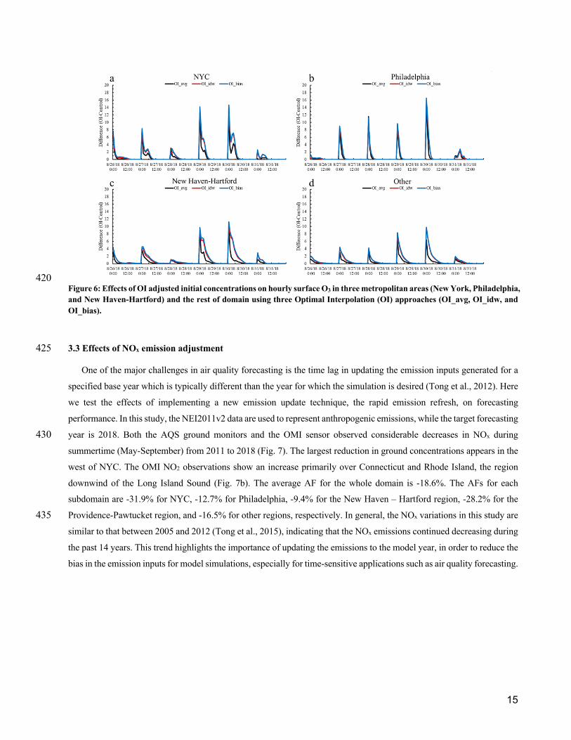
year is 2018. Both the AQS ground monitors and the OMI sensor observed considerable decreases in NOx during 430 summertime (May-September) from 2011 to 2018 (Fig. 7). The largest reduction in ground concentrations appears in the

west of NYC. The OMI NO2 observations show an increase primarily over Connecticut and Rhode Island, the region

downwind of the Long Island Sound (Fig. 7b). The average AF for the whole domain is -18.6%. The AFs for each

subdomain are -31.9% for NYC, -12.7% for Philadelphia, -9.4% for the New Haven – Hartford region, -28.2% for the

Providence-Pawtucket region, and -16.5% for other regions, respectively. In general, the NOx variations in this study are 435 similar to that between 2005 and 2012 (Tong et al., 2015), indicating that the NOx emissions continued decreasing during

the past 14 years. This trend highlights the importance of updating the emissions to the model year, in order to reduce the

bias in the emission inputs for model simulations, especially for time-sensitive applications such as air quality forecasting.

16

Figure 7: NOx differences observed by (a) AQS and (b) OMI from summer 2011 to summer 2018 over the LIS model domain. 440

The results in Table 4 and 5 show that the performance for O3 and NO2 prediction is very similar between two

simulations using the two emission adjustment methods (a uniform average adjustment factor over the entire domain, and

spatially varied factors for each subdomain defined in Figure 1). The correlations in each sub-domains are the same and

the average for both simulations is 0.81 for O3 and 0.69 for NO2, respectively. The biases and errors are also at the same 445 level from the two simulations. Compared to the O3 in the Control run, RMSE changes slightly from 14.97 ppbv to 14.71

ppbv (EmisAdj_avg) and 14.55 ppbv (EmisAdj_sub), while the correlation remains the same. The largest differences

appeared in NYC with RMSE of 15.54 (EmisAdj_avg) and 14.93 ppb (EmisAdj_sub). This demonstrates that emission

adjustment alone results in limited improvement of O3 prediction, due in part to the fact that the O3 production in this

region is NOx saturated (VOC limited) in urban areas where most AQS monitors are deployed, so the O3 level is less 450 sensitive to the change in NOx emissions. Similarly, the retrievals of satellite observations are also more sensitive to urban

plumes. In addition, regional transport of air pollution results in dispersion of emitted NOx and its byproducts/reservoirs.

The observations from satellite or ground monitors, based on which the emissions were adjusted, may not accurately

capture the temporal evolution of the emission sources. A large geographical range may better reflect the overall changes

of NOx emissions in the LIS region. Previous studies either use a coarse model resolution (e.g., 1 degree in Lamsal et al., 455 2011, or state-level adjustment in Tong et al., 2016). As a result, the simulated concentrations using different methods

were very close and the limited difference can also get averaged out when calculating the averaged statistical metrics.

The effect of the emission adjustment method in this study is not as large as BCON or OI adjustments, which directly

influence O3 concentrations. A recent study by Jin et al. (2020) showed that the decrease in NOx emissions has shifted

the NOx-saturated to NOx-sensitive regime transition zone closer to urban centers, approximately 40 to 60 km from the 460 center (the highest emission point) of New York City. Therefore, it is expected that the effectiveness of emission

adjustment will increase over time in this region. For surface NO2, the emission adjustment showed a more significant

impact on simulated concentrations. Note that the emission adjustment was only implemented in the LIS system, not in

NAQFC, which still uses the 2014 NEI for anthropogenic emissions. Without the emission adjustment, the changes in

NOx emissions between the inventory and forecast years are not accounted for. On the high O3 days, NAQFC over-465 predicted surface O3 during the study period (Fig. 2c). The NAQFC LBCs are likely associated with a possible over-

prediction of the regional transport, which can be partially responsible for the BCON LIS simulation overpredicting O3

17

during high O3 days (Fig 2d). Considering the similarities of these two emission adjustment methods, they will be both

tested in the subsequent multi-adjustment simulations.

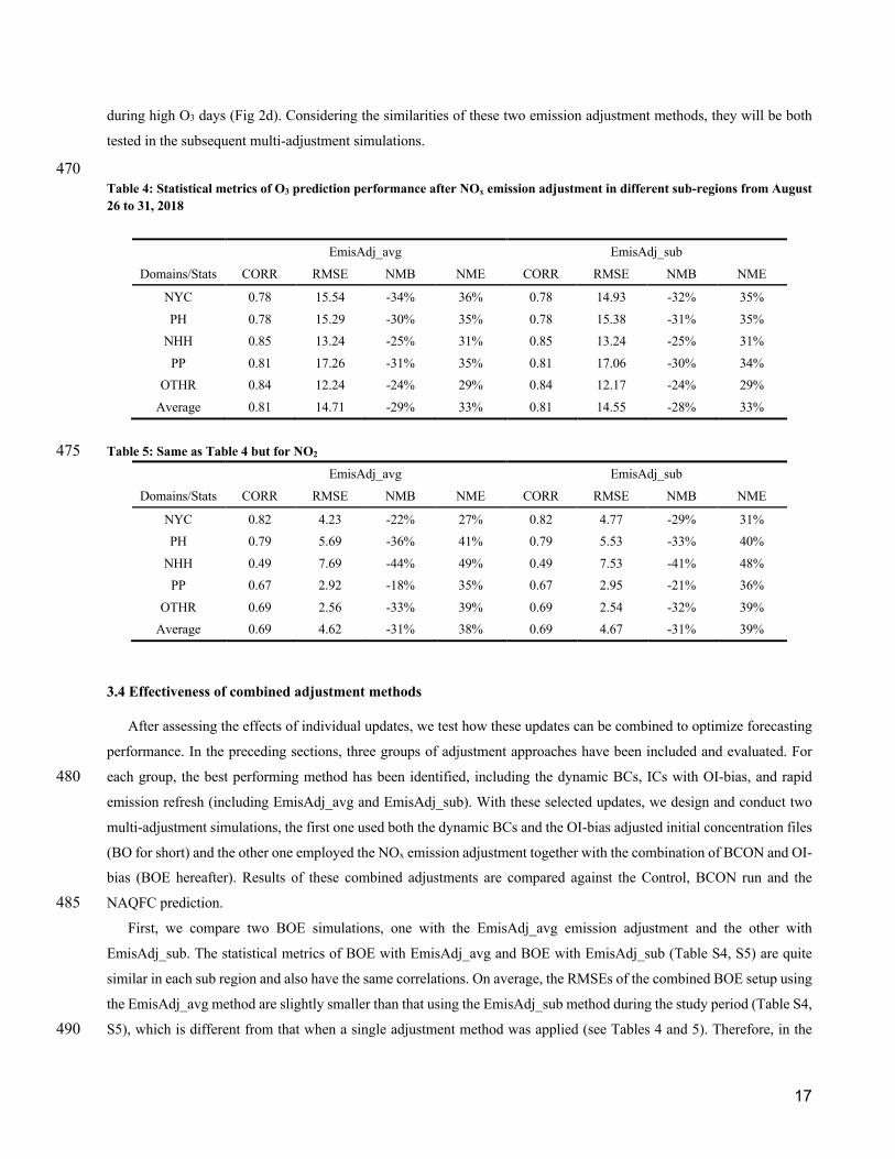
470 Table 4: Statistical metrics of O3 prediction performance after NOx emission adjustment in different sub-regions from August 26 to 31, 2018

EmisAdj_avg EmisAdj_sub

Domains/Stats CORR RMSE NMB NME CORR RMSE NMB NME

NYC 0.78 15.54 -34% 36% 0.78 14.93 -32% 35%

PH 0.78 15.29 -30% 35% 0.78 15.38 -31% 35% NHH 0.85 13.24 -25% 31% 0.85 13.24 -25% 31%

PP 0.81 17.26 -31% 35% 0.81 17.06 -30% 34% OTHR 0.84 12.24 -24% 29% 0.84 12.17 -24% 29%

Average 0.81 14.71 -29% 33% 0.81 14.55 -28% 33%

Table 5: Same as Table 4 but for NO2 475

EmisAdj_avg EmisAdj_sub

Domains/Stats CORR RMSE NMB NME CORR RMSE NMB NME

NYC 0.82 4.23 -22% 27% 0.82 4.77 -29% 31% PH 0.79 5.69 -36% 41% 0.79 5.53 -33% 40%

NHH 0.49 7.69 -44% 49% 0.49 7.53 -41% 48% PP 0.67 2.92 -18% 35% 0.67 2.95 -21% 36%

OTHR 0.69 2.56 -33% 39% 0.69 2.54 -32% 39% Average 0.69 4.62 -31% 38% 0.69 4.67 -31% 39%

3.4 Effectiveness of combined adjustment methods

After assessing the effects of individual updates, we test how these updates can be combined to optimize forecasting

performance. In the preceding sections, three groups of adjustment approaches have been included and evaluated. For

each group, the best performing method has been identified, including the dynamic BCs, ICs with OI-bias, and rapid 480 emission refresh (including EmisAdj_avg and EmisAdj_sub). With these selected updates, we design and conduct two

multi-adjustment simulations, the first one used both the dynamic BCs and the OI-bias adjusted initial concentration files

(BO for short) and the other one employed the NOx emission adjustment together with the combination of BCON and OI-

bias (BOE hereafter). Results of these combined adjustments are compared against the Control, BCON run and the

NAQFC prediction. 485 First, we compare two BOE simulations, one with the EmisAdj_avg emission adjustment and the other with

EmisAdj_sub. The statistical metrics of BOE with EmisAdj_avg and BOE with EmisAdj_sub (Table S4, S5) are quite

similar in each sub region and also have the same correlations. On average, the RMSEs of the combined BOE setup using

the EmisAdj_avg method are slightly smaller than that using the EmisAdj_sub method during the study period (Table S4,

S5), which is different from that when a single adjustment method was applied (see Tables 4 and 5). Therefore, in the 490

18

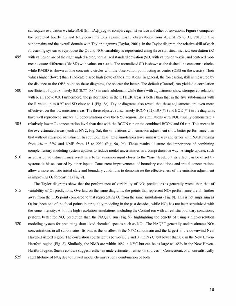
subsequent evaluation we take BOE (EmisAdj_avg) to compare against surface and other observations. Figure 8 compares

the predicted hourly O3 and NO2 concentrations against in-situ observations from August 26 to 31, 2018 in five

subdomains and the overall domain with Taylor diagrams (Taylor, 2001). In the Taylor diagram, the relative skill of each

forecasting system to reproduce the O3 and NO2 variability is represented using three statistical metrics: correlation (R)

with values on arc of the right angled sector, normalized standard deviation (SD) with values on y-axis, and centered root-495 mean-square difference (RMSD) with values on x-axis. The normalized SD is shown as the dashed line concentric circles

while RMSD is shown as line concentric circles with the observation point acting as center (OBS on the x-axis). Their

values higher (lower) than 1 indicate biased high (low) of the simulations. In general, the forecasting skill is measured by

the distance to the OBS point on these diagrams, the shorter the better. The default (Control) run yielded a correlation

coefficient of approximately 0.8 (0.77–0.84) in each subdomain while those with adjustments show stronger correlations 500 with R all above 0.9. Furthermore, the performance in the OTHER areas is better than that in the five subdomains with

the R value up to 0.97 and SD close to 1 (Fig. 8e). Taylor diagrams also reveal that these adjustments are even more

effective over the low emission areas. The three adjusted runs, namely BCON (#2), BO (#3) and BOE (#4) in the diagrams,

have well reproduced surface O3 concentrations over the NYC region. The simulations with BOE usually demonstrate a

relatively lower O3 concentration level than that with the BCON run or the combined BCON and OI run. This means in 505 the overestimated areas (such as NYC, Fig. 8a), the simulations with emission adjustment show better performance than

that without emission adjustment. In addition, these three simulations have similar biases and errors with NMB ranging

from 4% to 22% and NME from 15 to 22% (Fig. 9a, 9c). These results illustrate the importance of combining

complementary modeling system updates to reduce model uncertainties in a comprehensive way. A single update, such

as emission adjustment, may result in a better emission input closer to the “true” level, but its effect can be offset by 510 systematic biases caused by other inputs. Concurrent improvements of boundary conditions and initial concentrations

allow a more realistic initial state and boundary conditions to demonstrate the effectiveness of the emission adjustment

in improving O3 forecasting (Fig. 9).

The Taylor diagrams show that the performance of variability of NO2 predictions is generally worse than that of

variability of O3 predictions. Overlaid on the same diagrams, the points that represent NO2 performance are all further 515 away from the OBS point compared to that representing O3 from the same simulations (Fig. 8). This is not surprising as

O3 has been one of the focal points in air quality modeling in the past decades, while NO2 has not been scrutinized with

the same intensity. All of the high-resolution simulations, including the Control run with unrealistic boundary conditions,

perform better for NO2 prediction than the NAQFC run (Fig. 9), highlighting the benefit of using a high-resolution

modeling system for predicting short-lived chemical species such as NO2. The NAQFC generally underestimates NO2 520 concentrations in all subdomains. Its bias is the smallest in the NYC subdomain and the largest in the downwind New

Haven-Hartford region. The correlation coefficient is between 0.8 and 0.9 in NYC, but lower than 0.6 in the New Haven-

Hartford region (Fig. 8). Similarly, the NMB are within 10% in NYC but can be as large as -65% in the New Haven-

Hartford region. Such a contrast suggests either an underestimate of emission sources in Connecticut, or an unrealistically

short lifetime of NOx due to flawed model chemistry, or a combination of both. 525

19

Figure 8: Model performance in Taylor diagrams of hourly O3 (in red color) and NO2 (in blue color) simulated by five runs, 530 including the Control run, dynamic boundary conditions (BCON), boundary conditions with optimal interpolation (BCON+OI), and an all adjustment run including emission adjustment (BOE), and the operational NOAA national air quality forecast capability (NAQFC) run during the episode over five subdomains and the overall domain (Average). The comparison time is from August 26 to 31, 2018. 535

20

Figure 9: Comparisons of model performance for surface O3 (top row) and NO2 (bottom row) concentrations from five CMAQ

simulations against measurements from the Air Quality System monitors. These simulations include the Control run, dynamic 540 boundary conditions (BCON), boundary conditions with optimal interpolation (BCON+OI), and an all adjustment run

including emission adjustment (BCOI+OI+EmisAdj), and the operational NOAA national air quality forecast capability

(NAQFC) run during the episode over five subdomains. Two performance metrics are used here: normalized mean bias (NMB)

and normalized mean error (NME). The comparison time is from August 26 to 31, 2018.

4. High O3 episode simulations during the LISTOS field campaign 545

In this section, the newly developed high-resolution system, equipped with all forecast improvements (dynamic

Boundary conditions, Optimal interpolation, and Emission adjustment, or BOE), is used to simulate a high O3 episode

over the Long Island Sound region. During the high O3 pollution days (August 28-29, 2018) in this episode, surface O3

concentrations exceeded the National Ambient Air Quality Standard (NAAQS) (daily maximum 8-hour average of 70

ppbv) at several monitoring locations, including one site (Colliers Mills) in New Jersey, one site (Riverhead) in New 550 York, and five sites (Greenwich, Madison-Beach Road, Middletown-CVH-Shed, Stratford, and Westport) in Connecticut.

While merely exceeding the threshold values by a few ppbv at most sites, the O3 concentrations reached 84 ppbv at the

Westport site, and 87 ppbv at the Stratford site. Considering the significant emission reduction and air quality

improvements in the eastern United States (He et al., 2020; Qu et al., 2019), this episode, which occurred during a well-

designed field campaign, offers a rare opportunity to assess how well a state-of-the-science air quality model can predict 555 a high O3 pollution event that is now less frequent than in the past decades.

4.1 NO2 prediction

CMAQ predictions of NO2 surface concentrations and vertical column density are compared against ground and

aircraft observations. NO2 is not only a key precursor to tropospheric ozone, but also a proxy for traffic-related air

pollution in many epidemiological studies (e.g., Jerrett et al., 2007). Within the LISTOS CMAQ domain, there are four 560 active ground monitors with valid NO2 readings during the study period. Hourly variations from AQS monitors, the BOE

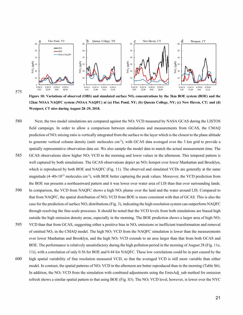
3 km prediction, and the operational NAQFC prediction are illustrated in Fig. 10. Among these sites, the lowest NO2

concentrations were observed at the Flax Pond site in the middle of Long Island, away from the major emission sources.

Both BOE and NAQFC are able to reproduce the magnitude and diurnal variations of surface NO2 concentrations at this

site. The NO2 concentration at the Queens College site, also located in the Long Island Sound and downtown NYC, is 565 significantly higher than at the Flax Pond site, due to its close proximity to major sources such as the tunnels, harbors and

highways. At this site, the BOE 3 km prediction is considerably better than that from the NAQFC prediction. Similarly,

the BOE prediction outperforms the NAQFC at the New Haven site in Connecticut, where the surface NO2 concentration

reaches 40 ppbv on August 28 and 55 ppbv on August 29, 2018. The NAQFC predicted concentration is constantly below

10 ppbv, severely underestimating the observations. In comparison, the BOE predicted concentrations are much closer to 570 the observations, although still underpredicting the latter. Finally, both models missed the first, primary peak on both

days at the Westport, CT site, which is strongly influenced by the NY City plume and sea breeze circulation.

21

575 Figure 10: Variations of observed (OBS) and simulated surface NO2 concentrations by the 3km BOE system (BOE) and the

12km NOAA NAQFC system (NOAA NAQFC) at (a) Flax Pond, NY; (b) Queens College, NY; (c) New Haven, CT; and (d)

Westport, CT sites during August 28–29, 2018.

Next, the two model simulations are compared against the NO2 VCD measured by NASA GCAS during the LISTOS 580 field campaign. In order to allow a comparison between simulations and measurements from GCAS, the CMAQ

prediction of NO2 mixing ratio is vertically integrated from the surface to the layer which is the closest to the plane altitude

to generate vertical column density (unit: molecules cm-2), with GCAS data averaged over the 3 km grid to provide a

spatially representative observation data set. We also sample the model data to match the actual measurement time. The

GCAS observations show higher NO2 VCD in the morning and lower values in the afternoon. This temporal pattern is 585 well captured by both simulations. The GCAS observations depict an NO2 hotspot over lower Manhattan and Brooklyn,

which is reproduced by both BOE and NAQFC (Fig. 11). The observed and simulated VCDs are generally at the same

magnitude (4–40´1015 molecules cm-2), with BOE better capturing the peak values. Moreover, the VCD prediction from

the BOE run presents a northeastward pattern and it was lower over water area of LIS than that over surrounding lands.

In comparison, the VCD from NAQFC shows a high NO2 plume over the land and the water around LIS. Compared to 590 that from NAQFC, the spatial distribution of NO2 VCD from BOE is more consistent with that of GCAS. This is also the

case for the prediction of surface NO2 distributions (Fig. 3), indicating the high-resolution system can outperform NAQFC

through resolving the fine-scale processes. It should be noted that the VCD levels from both simulations are biased high

outside the high emission density areas, especially in the morning. The BOE prediction shows a larger area of high NO2

VCD than that from GCAS, suggesting either a positive bias in NOx emissions or inefficient transformation and removal 595 of emitted NOx in the CMAQ model. The high NO2 VCD from the NAQFC simulation is lower than the measurements

over lower Manhattan and Brooklyn, and the high NO2 VCD extends to an area larger than that from both GCAS and

BOE. The performance is relatively unsatisfactory during the high pollution period in the morning of August 28 (Fig. 11e,

11i), with a correlation of only 0.56 for BOE and 0.44 for NAQFC. These low correlations could be in part caused by the

high spatial variability of fine resolution measured VCD, so that the averaged VCD is still more variable than either 600 model. In contrast, the spatial patterns of NO2 VCD in the afternoon are better reproduced than in the morning (Table S6).

In addition, the NO2 VCD from the simulation with combined adjustments using the EmisAdj_sub method for emission

refresh shows a similar spatial pattern to that using BOE (Fig. S3). The NO2 VCD level, however, is lower over the NYC

22

area suggesting an underestimate over the hotspot but much better prediction over the rest of the area. Besides the

uncertainties in the model, an evaluation conducted by Judd et al. (2020) showed that the absolute difference in GCAS 605 from Pandora measurements has an average and standard deviation of -0.2×1015±2×1015 molecules cm-2 and a percent

difference on average of -1.5%±20%. Overall, the BOE simulation at the 3 km resolution is able to reproduce the observed

NO2 VCD, and unlike the results of surface NO2, the NO2 VCD using EmisAdj_sub has lower NMB (33%) and NME

(57%) compared to that using EmisAdj_avg (40% and 61%) while their correlation is still the same (0.74). It indicates

the advantage of adjusting emission with a finer spatial resolution in simulating NO2 vertical column in this study. Table 610 S6 shows that both 3km simulations perform better than the 12 km NAQFC (R = 0.57, NMB = 45% and NME = 76%,

respectively).

615

Figure 11: Spatial distribution of NO2 vertical column density (VCD) observed by NASA GeoCAPE Airborne Simulator

(GCAS) (top row), and simulated by the 3 km BOE (center row) and 12 km NOAA NAQFC (bottom row) over the LIS domain

during August 28–29, 2018. There were two flight missions each day: the morning flight (AM) from ~11:00 to 15:00 UTC and

afternoon flight (PM) from ~16:00 to 20:00 UTC.

620

4.2 O3 prediction

One key result expected from the improved prediction system is better prediction of high O3 episodes, especially those

events that cause the exceedance of NAAQS. Here we compare the model performance between BOE and NAQFC at the

seven sites where the O3 concentrations exceeded the NAAQS. Compared to NAQFC, BOE demonstrates enhanced

23

prediction skills at all sites (Fig. 12). Note the comparisons may be attributed to the differences in meteorology, emission 625 and other factors. Although it is difficult to attribute the improvement quantitatively to each factor, the magnitude of O3

improvement from the base run to the BOE run is comparable to that of the overall reduced O3 bias, suggesting a

significant contribution from these improvement techniques. The results show that BOE can better capture peak O3 values

than NAQFC in the afternoon, a highly desired feature in predicting O3 exceedances. Hourly surface O3 concentrations

reached more than 100 ppbv at four Connecticut sites, including Greenwich, Westport, Middletown-CVH-Shed, and 630 Stratford. While neither BOE nor NAQFC is able to predict such high values, BOE reduces the bias by 10-20 ppbv during

peak hours at these sites. The improvement of peak O3 prediction is less significant on the other sites with lower observed

O3 concentration, but BOE still displays better performance than NAQFC. There are only three sites at which one or both

simulations overpredict peak O3 on the August 29, 2018. Compared to NAQFC, BOE shows larger over-prediction of the

peak O3 at the Greenwich site, but smaller overprediction at two other sites (Middletown and Westport). 635 Besides better peak prediction, BOE has also improved the prediction of the timing of peak O3. The peaks predicted

by BOE are two to three hours earlier than that by NAQFC, which agree better with the timing of the observed peaks (Fig.

12). The BOE peaks are narrower than the NAQFC ones, so that the former follows the observed O3 downslope and

avoids the positive biases during late afternoon and early evening. Finally, BOE has improved the prediction of low O3

concentrations and nighttime O3 valleys that are lower than those from NAQFC. Both simulations, however, are unable 640 to reproduce the extreme low nighttime values at several sites. Overall, the BOE simulation performs better in capturing

daytime O3 peaks and nighttime valleys, as well as the timing of both, with a mean correlation coefficient of 0.93

compared to 0.88 for the NAQFC simulation. This can be in part attributed to the high resolution of the LIS 3km system,

which can better resolve meteorology and emission variations. As the emissions and meteorological inputs play an

important role in determining the magnitude and timing of high peaks (Pan et al., 2017), high resolution data of both 645 emission and meteorology contributed to the improved the simulation of peak O3 value and its timing, especially over

urban areas (Figure 12).

24

650 Figure 12: Time series of observed (OBS) and simulated surface O3 concentrations by the 3km system with dynamic Boundary

conditions, OI initialization and Emission adjustment (BOE) and the 12km NOAA National Air Quality Forecast Capability

System (NAQFC) system at the seven sites where the National Ambient Air Quality Standard (NAAQS) for O3 were exceeded

during August 28–29, 2018: a. Colliers Mills; b. Riverhead; c. Greenwich; d. Madison-Beach Road; e. Middletown-CVH-Shed;

f. Stratford; and g. Westport. 655

Vertical profiles of O3 are compared between the Langley Mobile O3 Lidar (LMOL) observations and the CMAQ

simulations at the Westport site. As shown in Fig. 13, LMOL observations reveal that the O3 concentration in the planetary

boundary layer starts to build up around 16:00–17:00 UTC and high concentrations (>~70 ppbv), which extend to a height

of about 1.5 km, last until 23:00 UTC on August 28 and 29. This pattern is reproduced by both the BOE and NAQFC 660 simulations. Above the PBL, the variations of O3 concentrations are also captured by both simulations. O3 concentrations

in the free troposphere are more controlled by regional O3 production and transport than in the PBL. Consequently, the

structure and magnitude of the O3 profiles are very similar between the BOE and NAQFC simulations, since the BOE

simulation is driven by the dynamic boundary conditions derived from the same NAQFC simulation. Compared to that

from the LMOL observations, the predicted O3 concentrations from both runs are biased low above 800 hPa but biased 665 high below it. Between the two model simulations, the BOE run not only produces more O3 in the PBL, but also shows a

better temporal evolution of the PBL structure, with a short-lived high O3 peak and a PBL height peak between 20:00–

22:00 UTC on August 28, and persistent O3 and PBL height plateaus between 16:00–23:00 UTC on August 29 (Fig. 13).

The PBL in the BOE simulation extends well above 850 mbar, while the observed high O3 from LMOL generally stays

beneath this height, suggesting possible overprediction of the PBL height. 670 In general, the 3 km BOE simulation performs better to capture the temporal variability of the PBL and O3 production

but tends to overestimate both during this episode. In contrast, the NAQFC simulation has produced less pronounced

25

temporal variations in both O3 concentrations and PBL height in the lower troposphere, in particular on August 28 when

this region experienced the worst air quality in several states. The NAQFC simulation, however, performed better during

the time with lower O3 concentrations, which resulted in an overall lower NMB (9%) and NME (21%) comparing to that 675 in BOE (22% and 26% respectively). The BOE simulation, however, presented a much better reproduction of the O3

variability in term of correlation (0.71) than the NAQFC run (0.54). This suggests that the new 3 km BOE system is more

responsive to the variations of the controlling factors that shape O3 pollution, although the system needs to be further

refined to reduce bias. The model performance for O3 surface concentration and vertical distribution using the AFs from

EmisAdj_sub is very close to those of using the AFs from EmisAdj_avg in the BOE case (Fig. S4, Table S7). 680

Figure 13: Comparison of vertical O3 profiles (observed by NASA Langley Mobile O3 Lidar (left column, a & d) with these

simulated by the 3 km prediction system (central column, b & e) and the 12 km NOAA NAQFC (right column, c & f) over the

Westport site on August 28 (upper row) and August 29, 2018 (lower row), respectively. Note white represents missing data 685 from the Lidar data.

5. Summary

Improvement of air quality in the past decades renders the prediction of high ozone events more challenging. This

study investigates the feasibility of designing a high-resolution air quality prediction system to capture these less frequent

events with more accuracy. Relying on the observations collected during the Long Island Sound Tropospheric Ozone 690 Study field campaign, we have assessed the effectiveness of various improvements to the prediction system to enhance

the predictability of high O3 episodes. These updates were then combined to explore how to further improve the

predictability of both ozone and nitrogen dioxide. Finally, the modeling system with combined updates has been utilized

to simulate a severe high O3 pollution event in the Long Island Sound and surrounding areas.

26

Different prediction system updates demonstrate varying potentials to improve O3 and NO2 prediction performance. 695 For O3 prediction, the most significant improvement comes from the dynamic boundary conditions derived from NOAA

National Air Quality Forecast Capability (NAQFC), compared to that with the static boundary conditions. This is due in

part to the fact that the relatively small model domain used in this study and that O3 is a regional air pollutant, making the

its prediction more susceptible to the influence of regional transport. Dynamic boundary conditions (BCs) are less

influential for NO2 prediction, for which all high-resolution simulations outperform the 12 km NAQFC simulation, 700 highlighting the importance of spatially resolved emission and meteorology for the prediction of short-lived pollutants.

The impact of improved initial concentrations through optimal interpolation (OI) is shown to be large in urban areas

initially but fades away rapidly. The influence of OI adjustment, however, lingers for a longer period in an area with low

emission density where emissions and chemical reactions make a smaller contribution to the O3 budget than that in the

areas with high emission density. Such method may be more useful if applied to vertical layers above the ground. Future 705 air quality forecasting and modeling can benefit from concerted efforts to provide near real time data of O3 aloft on a

continuous basis (Mathur et al., 2018), so that improved initialization of the aloft conditions can better represent regional

transport and modulate the inferred impact of LBCs on O3 prediction. Finally, emission adjustment, which changes the

baseline emissions using the temporal trends derived from ground and satellite observations, only yields moderate

improvement in O3 prediction compared to that without emission adjustment. One possible direction to explore is to apply 710 other methods to constrain emissions that use both variational (e.g., Elbern et al., 2007; Vira and Sofiev, 2012) and

ensemble-based (e.g., Miyazaki et al., 2012, 2017) solutions to analyze the 3D chemical tracers as well as their respective

precursor emissions simultaneously. In addition, the importance of volatile consumer product VOCs has been identified

in recent studies (McDonald et al., 2018), suggesting that updating other species than NOx is also necessary. This may be

challenging, however, through a similar approach to the NOx emission adjustment implemented here, since there are 715 limited measurements of VOCs from both ground and space instruments. While the effectiveness of each update varies,

a combination of these updates proves to outperform that with each single update. The new prediction system at 3 km

resolution, equipped with dynamic BCs, OI and Emission adjustment (BOE), was used to simulate a high O3 episode over

the Long Island Sound region. Compared to the 12km operational NAQFC, the BOE system is able to significantly reduce

the biases in surface O3 and NO2 prediction. The BOE is also able to reproduce NO2 VCD observed by NASA Langley 720 GCAS with higher accuracy than the NAQFC. More importantly, the BOE simulation shows considerable improvement

in capturing the O3 peaks and valleys, as well as the timing of both, with a correlation coefficient of 0.93 compared to

that of 0.88 by the NAQFC. This study demonstrates feasible measures to improve the capability of air quality prediction

systems to capture high O3 episodes in a cleaner urban environment.

725

Data Availability. WRF is an open-source community model. The source code is available at

http://www2.mmm.ucar.edu/wrf/users/download/get_source.html (last access: September 2021). CMAQ and SMOKE

source code is available on the Community Modeling and Analysis System (CMAS) Center of University of North

Carolina, Chapel Hill: https://www.cmascenter.org/ (last access: July 31, 2021). The AirNow hourly data of O3 and NOx 730 are available at https://files.airnowtech.org/?prefix=airnow/ (last access: May 2021) and the hourly NOx data from US

27

EPA Air Quality System (AQS) surface network is available at https://aqs.epa.gov/aqsweb/airdata/download_files.html

(last access: May 2021). The GCAS NO2 vertical column density and the LMOL O3 vertical profile data are available at

https://www-air.larc.nasa.gov/missions/listos/index.html (last access: May 2021). The monthly product of NO2 vertical

column density from OMI is available at https://avdc.gsfc.nasa.gov/pub/data/satellite/Aura/OMI (last access: July 31, 735 2021).

Author Contribution. DT and SM designed the study, conducted the simulations and wrote the manuscript. JW, XZ and

PL helped development of the modeling system. LL, RS and LJ provided OMI and LISTOS field campaign data and

helped interpreting the results. YT and TC provided code for the original OI method. All authors edited and commented 740 on the manuscript. All authors read, revised, and approved the final paper.

Competing interests. The authors declare that they have no conflict of interest.

Acknowledgement. This work was partially supported by a National Research Council fellowship to S. Ma at NOAA 745 Air Resources Laboratory and by NOAA Weather Program Office and Robert Wood Johnson Foundation to D. Tong.

The authors are grateful to the EPA and NYDEC for sharing the AQS data and to NASA for providing the OMI, GCAS

and Langley Mobile O3 Lidar datasets. Finally, we want to thank the Editor for handling our submission and two

anonymous reviewers for their constructive comments on earlier versions of this paper.

750

References

Adhikary, B., Kulkarni, S., Dallura, A., Tang, Y., Chai, T., Leung, L. R., Qian, Y., Chung, C. E., Ramanathan, V. and

Carmichael, G. R.: A regional scale chemical transport modeling of Asian aerosols with data assimilation of AOD

observations using optimal interpolation technique, Atmos. Environ., 42(37), 8600–8615,

https://doi.org/10.1016/j.atmosenv.2008.08.031, 2008. 755 Baker, K. R., Liljegren, J., Valin, L., Judd, L. M., Henderson, B. H., Szykman, J., Al-Saadi, J. A., Janz, S. J., Sareen, N.

and Possiel, N.: Model-Measurement Comparison of Ozone and Precursors Along Land-Water Interfaces during the

2017 LMOS and 2018 LISTOS Field Campaigns, AGUFM, 2019, A21E-06, 2019.

Berkoff, T., Gronoff, G., Baker, B., Lee, P., Dreessen, J. and Sullivan, J.: Comparison of tropospheric ozone vertical

profiles between NASA ozone lidars and NOAA’s National Air Quality Forecasting Capability (NAQFC) model, 760 AGUFM, 2019, A21E-02, https://doi.org/10.1016/j.atmosenv.2010.04.044, 2019.

Borge, R., López, J., Lumbreras, J., Narros, A. and Rodríguez, E.: Influence of boundary conditions on CMAQ

simulations over the Iberian Peninsula, Atmos. Environ., 44(23), 2681–2695,

https://doi.org/10.1016/j.atmosenv.2010.04.044, 2010.

Brunekreef, B. and Holgate, S. T.: Air pollution and health, Lancet, 360(9341), 1233–1242, 765 https://doi.org/10.1016/S0140-6736(02)11274-8, 2002.

28

Byun, D. and Schere, K. L.: Review of the governing equations, computational algorithms, and other components of the

Models-3 Community Multiscale Air Quality (CMAQ) modeling system, https://doi.org/10.1115/1.2128636, 2006.

Candiani, G., Carnevale, C., Finzi, G., Pisoni, E. and Volta, M.: A comparison of reanalysis techniques: Applying optimal

interpolation and Ensemble Kalman Filtering to improve air quality monitoring at mesoscale, Sci. Total Environ., 458, 770 7–14, https://doi.org/10.1016/j.scitotenv.2013.03.089, 2013.

Chai, T., Kim, H., Pan, L., Lee, P. and Tong, D.: Impact of Moderate Resolution Imaging Spectroradiometer aerosol

optical depth and AirNow PM2. 5 assimilation on Community Multi‐scale Air Quality aerosol predictions over the

contiguous United States, J. Geophys. Res. Atmos., 122(10), 5399–5415, https://doi.org/10.1002/2016JD026295,

2017. 775 Chameides, W. L., Fehsenfeld, F., Rodgers, M. O., Cardelino, C., Martinez, J., Parrish, D., Lonneman, W., Lawson, D.

R., Rasmussen, R. A. and Zimmerman, P.: Ozone precursor relationships in the ambient atmosphere, J. Geophys. Res.

Atmos., 97(D5), 6037–6055, 1992.

Davidson, P., Schere, K., Draxler, R., Kondragunta, S., Wayland, R. A., Meagher, J. F., and Mathur, R.: Toward a US

National Air Quality Forecast Capability: Current and Planned Capabilities, in: Air Pollution Modeling and Its 780 Application XIX, edited by: Borrego, C. and Miranda, A., pp. 226–234, Springer, Dordrecht, The Netherlands, 2008.

De Young, R., Carrion, W., Ganoe, R., Pliutau, D., Gronoff, G., Berkoff, T. and Kuang, S.: Langley mobile ozone lidar:

ozone and aerosol atmospheric profiling for air quality research, Appl. Opt., 56(3), 721–730,

https://doi.org/10.1364/AO.56.000721, 2017.

Dix, B., de Bruin, J., Roosenbrand, E., Vlemmix, T., Francoeur, C., Gorchov‐Negron, A., McDonald, B., Zhizhin, M., 785 Elvidge, C. and Veefkind, P.: Nitrogen Oxide Emissions from US Oil and Gas Production: Recent Trends and Source

Attribution, Geophys. Res. Lett., 47(1), e2019GL085866, https://doi.org/10.1029/2019GL085866, 2020.

Dunlea, E. J., Herndon, S. C., Nelson, D. D., Volkamer, R. M., San Martini, F., Sheehy, P. M., Zahniser, M. S., Shorter,

J. H., Wormhoudt, J. C. and Lamb, B. K.: Evaluation of nitrogen dioxide chemiluminescence monitors in a polluted

urban environment, https://doi.org/10.5194/acp-7-2691-2007, 2007. 790 Eder, B., Kang, D., Rao, S. T., Mathur, R., Yu, S. C., Otte, T., Schere, K., Wayland, R., Jackson, S., Davidson, P., and

McQueen, J.: A demonstration of the use of national air quality forecast guidance for developing local air quality

index forecasts, B. Am. Meteorol. Soc., 91, 313–326, doi:10.1175/2009BAMS2734.1, 2010.

Elbern, H., Strunk, A., Schmidt, H., and Talagrand, O.: Emission rate and chemical state estimation by 4-dimensional

variational inversion, Atmos. Chem. Phys., 7, 3749–3769, https://doi.org/10.5194/acp-7-3749-2007, 2007. 795 Feng, J., Chan, E., and Vet, R.: Air quality in the eastern United States and Eastern Canada for 1990–2015: 25 years of

change in response to emission reductions of SO2 and NOx in the region, Atmos. Chem. Phys., 20, 3107–3134,

https://doi.org/10.5194/acp-20-3107-2020, 2020.

Fiore, A. M., Dentener, F. J., Wild, O., Cuvelier, C., Schultz, M. G., Hess, P., Textor, C., Schulz, M., Doherty, R. M. and Horowitz, L. W.: Multimodel estimates of intercontinental source‐receptor relationships for ozone pollution, J. 800 Geophys. Res. Atmos., 114(D4), 2009.

Gantt, B., Kelly, J. T. and Bash, J. O.: Updating sea spray aerosol emissions in the Community Multiscale Air Quality

(CMAQ) model version 5.0. 2., Geosci. Model Dev. Discuss., 8(5), https://doi.org/10.5194/gmd-8-3733-2015, 2015.

29

Gong, S. L.: A parameterization of sea‐salt aerosol source function for sub‐and super‐micron particles, Global

Biogeochem. Cycles, 17(4), https://doi.org/10.1029/2003GB002079, 2003. 805 Gronoff, G., Robinson, J., Berkoff, T., Swap, R., Farris, B., Schroeder, J., Halliday, H. S., Knepp, T., Spinei, E. and

Carrion, W.: A method for quantifying near range point source induced O3 titration events using Co-located Lidar and

Pandora measurements, Atmos. Environ., 204, 43–52, https://doi.org/10.1016/j.atmosenv.2019.01.052, 2019.

He, H., Liang, X.-Z., Sun, C., Tao, Z. and Tong, D. Q.: The long-term trend and production sensitivity change in the US

ozone pollution from observations and model simulations., Atmos. Chem. Phys., 20(5), https://doi.org/10.5194/acp-810 20-3191-2020, 2020.

Henderson, B. H., Akhtar, F., Pye, H. O. T., Napelenok, S. L. and Hutzell, W. T.: A database and tool for boundary

conditions for regional air quality modeling: description and evaluation, Geosci. Model Dev., 7(1), 339–360,

https://doi.org/10.5194/gmd-7-339-2014, 2014.

Héroux, M.-E., Anderson, H. R., Atkinson, R., Brunekreef, B., Cohen, A., Forastiere, F., Hurley, F., Katsouyanni, K., 815 Krewski, D. and Krzyzanowski, M.: Quantifying the health impacts of ambient air pollutants: recommendations of a

WHO/Europe project, Int. J. Public Health, 60(5), 619–627, https://doi.org/10.1007/s00038-015-0690-y, 2015.

Hogrefe, C., Hao, W., Civerolo, K., Ku, J.-Y., Sistla, G., Gaza, R. S., Sedefian, L., Schere, K., Gilliland, A. and Mathur,

R.: Daily simulation of ozone and fine particulates over New York State: findings and challenges, J. Appl. Meteorol.

Climatol., 46(7), 961–979, 2007. 820 Hogrefe, C., Hao, W., Zalewsky, E., Ku, J., Lynn, B., Rosenzweig, C., Schultz, M. G., Rast, S., Newchurch, M. J. and

Wang, L.: An analysis of long-term regional-scale ozone simulations over the Northeastern United States: variability

and trends, Atmos. Chem. Phys., 11(2), 23045–23090, doi:10.5194/acp-11-567-2011, https://doi.org/10.5194/acp-11-

567-2011, 2011.

Houyoux, M., Vukovich, J., Brandmeyer, J. E., Seppanen, C. and Holland, A.: Sparse matrix operator kernel emissions 825 modeling system-SMOKE User manual, Prep. by MCNC-North Carolina Supercomputing Center, Environ. Programs,

Res. Triangle Park. NC, 2000.

Jerrett, M., Arain, M. A., Kanaroglou, P., Beckerman, B., Crouse, D., Gilbert, N. L., Brook, J. R., Finkelstein, N. and

Finkelstein, M. M.: Modeling the intraurban variability of ambient traffic pollution in Toronto, Canada, J. Toxicol.

Environ. Heal. Part A, 70(3–4), 200–212, https://doi.org/10.1080/15287390600883018, 2007. 830 Jin, X., Fiore, A., Boersma, K. F., Smedt, I. D. and Valin, L., Inferring Changes in Summertime Surface Ozone–NOx–

VOC Chemistry over US Urban Areas from Two Decades of Satellite and Ground-Based Observations. Environ. Sci.

Technol., 54(11), 6518-6529, https://doi.org/10.1021/acs.est.9b07785, 2020.

Judd, L. M., Al-Saadi, J. A., Szykman, J. J., Valin, L. C., Janz, S. J., Kowalewski, M. G., Eskes, H. J., Veefkind, J. P.,

Cede, A., Mueller, M., Gebetsberger, M., Swap, R., Pierce, R. B., Nowlan, C. R., Abad, G. G., Nehrir, A., and 835 Williams, D.: Evaluating Sentinel-5P TROPOMI tropospheric NO2 column densities with airborne and Pandora

spectrometers near New York City and Long Island Sound, Atmos. Meas. Tech., 13, 6113–6140,

https://doi.org/10.5194/amt-13-6113-2020, 2020.

Kim, J. Y., Burnett, R. T., Neas, L., Thurston, G. D., Schwartz, J., Tolbert, P. E., Brunekreef, B., Goldberg, M. S. and

Romieu, I.: Panel discussion review: session two—interpretation of observed associations between multiple ambient 840

30

air pollutants and health effects in epidemiologic analyses, J. Expo. Sci. Environ. Epidemiol., 17(2), S83–S89, Panel

discussion review: session two—interpretation of observed associations between multiple ambient air pollutants and

health effects in epidemiologic analyses, 2007.

Kowalewski, M. G. and Janz, S. J.: Remote sensing capabilities of the GeoCAPE Airborne Simulator, in Earth Observing

Systems XIX, vol. 9218, p. 92181I, International Society for Optics and Photonics., 845 https://doi.org/10.1117/12.2062058, 2014.

Krotkov, N. A., McLinden, C. A., Li, C., Lamsal, L. N., Celarier, E. A., Marchenko, S. V, Swartz, W. H., Bucsela, E. J.,

Joiner, J. and Duncan, B. N.: Aura OMI observations of regional SO 2 and NO 2 pollution changes from 2005 to 2015,

Atmos. Chem. Phys., 16(7), 4605, 2016.

Khan, A.W., Kumar, P., Impact of chemical initial and lateral boundary conditions on air quality prediction. Adv. Sp. Res. 850 64, 1331–1342, https://doi.org/10.1016/j.asr.2019.06.028, 2019.

Lamsal, L. N., Martin, R. V., Padmanabhan, A., Van Donkelaar, A., Zhang, Q., Sioris, C. E., K. Chance, T. P. Kurosu,

Newchurch, M. J. Application of satellite observations for timely updates to global anthropogenic NOx emission

inventories. Geophysical Research Letters, 38(5), https://doi.org/10.1029/2010GL046476, 2011.

Lamsal, L. N., Krotkov, N. A., Vasilkov, A., Marchenko, S., Qin, W., Yang, E.-S., Fasnacht, Z., Joiner, J., Choi, S., 855 Haffner, D., Swartz, W. H., Fisher, B., and Bucsela, E.: OMI/Aura Nitrogen Dioxide Standard Product with Improved

Surface and Cloud Treatments, Atmos. Meas. Tech. Discuss., https://doi.org/10.5194/amt-2020-200, in review, 2020.

Lee, P., McQueen, J., Stajner, I., Huang, J., Pan, L., Tong, D., Kim, H., Tang, Y., Kondragunta, S. and Ruminski, M.:

NAQFC developmental forecast guidance for fine particulate matter (PM2. 5), Weather Forecast., 32(1), 343–360,

https://doi.org/10.1175/WAF-D-15-0163.1, 2017. 860 Lee, S.-H., Kim, S.-W., Trainer, M., Frost, G. J., McKeen, S. A., Cooper, O. R., Flocke, F., Holloway, J. S., Neuman, J.

A. and Ryerson, T.: Modeling ozone plumes observed downwind of New York City over the North Atlantic Ocean

during the ICARTT field campaign., Atmos. Chem. Phys. Discuss., 11(5), https://doi.org/10.5194/acp-11-7375-2011,

2011.

Levelt, P. F., van den Oord, G. H. J., Dobber, M. R., Malkki, A., Visser, H., de Vries, J., Stammes, P., Lundell, J. O. V 865 and Saari, H.: The ozone monitoring instrument, IEEE Trans. Geosci. Remote Sens., 44(5), 1093–1101,

https://doi.org/10.1109/TGRS.2006.872333, 2006.

Liu, T.-H., Jeng, F.-T., Huang, H.-C., Berge, E. and Chang, J. S.: Influences of initial conditions and boundary conditions

on regional and urban scale Eulerian air quality transport model simulations, Chemosphere-Global Chang. Sci., 3(2),

175–183, https://doi.org/10.1016/S1465-9972(00)00048-9, 2001. 870 Long, R., Hall, E., Beaver, M., Duvall, R., Kaushik, S., Kronmiller, K., Wheeler, M., Garvey, S., Drake, Z. and McElroy,

F.: Performance of the Proposed New Federal Reference Methods for Measuring Ozone Concentrations in Ambient

Air. US Environmental Protection Agency. Washington, DC, EPA/600/R-14/432 (NTIS PB2015e101240), 2014.

Lu, Z., Streets, D. G., de Foy, B., Lamsal, L. N., Duncan, B. N., and Xing, J.: Emissions of nitrogen oxides from US urban

areas: estimation from Ozone Monitoring Instrument retrievals for 2005–2014, Atmos. Chem. Phys., 15, 10367–10383, 875 https://doi.org/10.5194/acp-15-10367-2015, 2015.

31

Luecken, D. J., Yarwood, G. and Hutzell, W. T.: Multipollutant modeling of ozone, reactive nitrogen and HAPs across

the continental US with CMAQ-CB6, Atmos. Environ., 201, 62–72, https://doi.org/10.1016/j.atmosenv.2018.11.060,

2019.

Makar, P. A., Gong, W., Mooney, C., Zhang, J., Davignon, D., Samaali, M., Moran, M. D., He, H., Tarasick, D. W. and 880 Sills, D.: Dynamic adjustment of climatological ozone boundary conditions for air-quality forecasts, Atmos. Chem.

Phys. Discuss., 10(6), 13643–13688, https://doi.org/10.5194/acp-10-8997-2010, 2010.

Mathur, R., C. Hogrefe, A. Hakami, S. Zhao, J. Szykman, and G. Hagler.: A call for an aloft air quality monitoring

network: need, feasibility, and potential value. Environ. Sci. Technol, 52 (19), 10903–10908,

https://doi.org/10.1021/acs.est.8b02496, 2018. 885 McClenny, W. A., Williams, E. J., Cohen, R. C. and Stutz, J.: Preparing to measure the effects of the NOX SIP Call—

methods for ambient air monitoring of NO, NO2, NOY, and individual NOZ species, J. Air Waste Manage. Assoc.,

52(5), 542–562, https://doi.org/10.1080/10473289.2002.10470801, 2002.

McDonald, B. C., de Gouw, J. A., Gilman, J. B., Jathar, S. H., Akherati, A., Cappa, C. D., Jimenez, J. L., Lee-Taylor, J.,

Hayes, P. L., McKeen, S. A., Cui, Y. Y., Kim, S.-W., Gentner, D. R., Isaacman-VanWertz, G., Goldstein, A. H., 890 Harley, R. A., Frost, G. J., Roberts, J. M., Ryerson, T. B., and Trainer, M.: Volatile chemical products emerging as

largest petrochemical source of urban organic emissions, Science, 359, 760–764,

https://doi.org/10.1126/science.aaq0524, 2018.

Miyazaki, K., Eskes, H. J., and Sudo, K.: Global NOx emission estimates derived from an assimilation of OMI

tropospheric NO2 columns, Atmos. Chem. Phys., 12, 2263–2288, https://doi.org/10.5194/acp-12-2263-2012, 2012. 895 Miyazaki, K., Eskes, H., Sudo, K., Boersma, K. F., Bowman, K., and Kanaya, Y.: Decadal changes in global surface NOx

emissions from multi-constituent satellite data assimilation, Atmos. Chem. Phys., 17, 807–837,

https://doi.org/10.5194/acp-17-807-2017, 2017.

National Research Council: Rethinking the ozone problem in urban and regional air pollution, National Academies Press.,

1992. 900 Nowlan, C. R., Liu, X., Janz, S. J., Kowalewski, M. G., Chance, K., Follette-Cook, M. B., Fried, A., Abad, G. G., Herman,

J. R. and Judd, L. M.: Nitrogen dioxide and formaldehyde measurements from the GEOstationary Coastal and Air

Pollution Events (GEO-CAPE) airborne simulator over Houston, Texas, https://doi.org/10.5194/amt-2018-156, 2018,

2018.

Oliveri Conti, G., Heibati, B., Kloog, I., Fiore, M., Ferrante, M. A review of Air QModels and their applications for 905 forecasting the air pollution health outcomes.Environ. Sci. Pollut. Res.http://dx.doi.org/10.1007/s11356-016-8180-1,

2017.

Pan, L., Tong, D., Lee, P., Kim, H.-C. and Chai, T.: Assessment of NOx and O3 forecasting performances in the US

National Air Quality Forecasting Capability before and after the 2012 major emissions updates, Atmos. Environ., 95,

610–619, https://doi.org/10.1016/j.atmosenv.2014.06.020, 2014. 910 Pan, S., Choi, Y., Jeon, W., Roy, A., Westenbarger, D. A., and Kim, H. C.: Impact of high-resolution sea surface

temperature, emission spikes and wind on simulated surface ozone in Houston, Texas during a high ozone episode,

Atmos. Environ., 152, 362–376, https://doi.org/10.1016/j.atmosenv.2016.12.030, 2017.

32

Pierce, T., Geron, C., Bender, L., Dennis, R., Tonnesen, G. and Guenther, A.: Influence of increased isoprene emissions

on regional ozone modeling, J. Geophys. Res. Atmos., 103(D19), 25611–25629, 1998. 915 Pour‐Biazar, A., Khan, M., Wang, L., Park, Y., Newchurch, M., McNider, R. T., Liu, X., Byun, D. W. and Cameron,

R.: Utilization of satellite observation of ozone and aerosols in providing initial and boundary condition for regional

air quality studies, J. Geophys. Res. Atmos., 116(D18), https://doi.org/10.1029/2010JD015200, 2011.

Qu, Z.; Henze, D.K.; Li, C.; Theys, N.; Wang, Y.; Wang, J.; Wang, W.; Han, J.; Shim, C.; Dickerson, R.R.; Ren, X., SO₂

Emission Estimates Using OMI SO₂ Retrievals for 2005‐2017. , Journal of Geophysical Research: Atmospheres, 920

Vol. 124, Issue 4, 8336-8359, https://doi.org/10.1029/2019JD030243, 2019.

Sandu, A., Chai, T. and Carmichael, G. R.: Integration of Models and Observations–a Modern Paradigm for Air Quality

Simulations, Model. Pollut. Complex Environ. Syst., 2, 419, 2010.

Shepard, D., A two-dimensional interpolation function for irregularly-spaced data, in: Proceedings of the 1968 23rd ACM

National Conference. 517–524, https://doi.org/10.1145/800186.810616, 1968. 925 Shu, Q., Baker, K. R., Napelenok, S. L., Szykman, J., Valin, L. and Plessel, T.: Multi-scale Analysis of Ozone Source

Apportionment Using CMAQ-ISAM during 2018 LISTOS Field Campaign, AGUFM, 2019, A31E-06, 2019.

Silvern, R. F., Jacob, D. J., Mickley, L. J., Sulprizio, M. P., Travis, K. R., Marais, E. A., Cohen, R. C., Laughner, J. L.,

Choi, S. and Joiner, J.: Using satellite observations of tropospheric NO_2 columns to infer long-term trends in US

NO_x emissions: the importance of accounting for the free tropospheric NO_2 background, Atmos. Chem. Phys., 930 19(13), 8863–8878, https://doi.org/10.5194/acp-19-8863-2019, 2019.

Simon, H., Reff, A., Wells, B., Xing, J. and Frank, N.: Ozone trends across the United States over a period of decreasing

NOx and VOC emissions, Environ. Sci. Technol., 49(1), 186–195, https://doi.org/10.1021/es504514z, 2015.

Skamarock, W. C., Klemp, J. B., Dudhia, J., Gill, D. O., Barker, D. M., Wang, W. and Powers, J. G.: A description of the

advanced research WRF version 2, National Center For Atmospheric Research Boulder Co Mesoscale and Microscale, 935 https://doi.org/10.5065/1dfh-6p972005.

Spicer, C. W.: Smog chamber studies of nitrogen oxide (NOx) transformation rate and nitrate precursor relationships,

Environ. Sci. Technol., 17(2), 112–120, https://doi.org/10.1021/es00108a010, 1983.

Sullivan, J. T., Berkoff, T., Gronoff, G., Knepp, T., Pippin, M., Allen, D., Twigg, L., Swap, R., Tzortziou, M. and

Thompson, A. M.: The Ozone Water–Land Environmental Transition Study, UMBC Fac. Collect., 940 https://doi.org/10.1175/BAMS-D-18-0025.1, 2019.Tang, Y. H., Pagowski, M., Chai, T. F., Pan, L., Lee, P., Baker, B.,

Kumar, R., Delle Monache, L., Tong, D. and Kim, H.-C.: A case study of aerosol data assimilation with the

Community Multi-scale Air Quality Model over the contiguous United States using 3D-Var and optimal interpolation

methods, 2017.

Taghavi, M., Cautenet, S., and Foret, G.: Simulation of ozone production in a complex circulation region using nested 945 grids, Atmos. Chem. Phys., 4, 825–838, https://doi.org/10.5194/acp-4-825-2004, 2004.

Tang, Y., Carmichael, G. R., Thongboonchoo, N., Chai, T., Horowitz, L. W., Pierce, R. B., Al‐Saadi, J. A., Pfister, G.,

Vukovich, J. M. and Avery, M. A.: Influence of lateral and top boundary conditions on regional air quality prediction:

A multiscale study coupling regional and global chemical transport models, J. Geophys. Res. Atmos., 112(D10),

https://doi.org/10.1029/2006JD007515, 2007. 950

33

Tang, Y., Chai, T., Pan, L., Lee, P., Tong, D., Kim, H.-C. and Chen, W.: Using optimal interpolation to assimilate surface

measurements and satellite AOD for ozone and PM2. 5: A case study for July 2011, J. Air Waste Manage. Assoc.,

65(10), 1206–1216, https://doi.org/10.1080/10962247.2015.1062439, 2015.

Tang, Y., Lee, P., Tsidulko, M., Huang, H.-C., McQueen, J. T., DiMego, G. J., Emmons, L. K., Pierce, R. B., Thompson,

A. M. and Lin, H.-M.: The impact of chemical lateral boundary conditions on CMAQ predictions of tropospheric 955 ozone over the continental United States, Environ. fluid Mech., 9(1), 43–58, https://doi.org/10.1007/s10652-008-

9092-5, 2009.

Tang, Y.H., Pagowski, M., Chai, T.F., Pan, L., Lee, P., Baker, B., Kumar, R., Delle Monache, L., Tong, D., Kim, H.-C.,

A case study of aerosol data assimilation with the Community Multi-scale Air Quality Model over the contiguous

United States using 3D-Var and optimal interpolation methods, Geosci. Model Dev., 10, 4743–4758, 960 https://doi.org/10.5194/gmd-10-4743-2017, 2017.

Taylor, K. E.: Summarizing multiple aspects of model performance in a single diagram, J. Geophys. Res. Atmos., 106(D7),

7183–7192, https://doi.org/10.1029/2000JD900719, 2001.

Tong, D. and Y. Tang. Advancing Air Quality Forecasting to Protect Human Health. Environmental Managers, October

2018, Available online at: https://pubs.awma.org/flip/EM-Oct-2018/tong.pdf. (accessed on 11.13.20) 965 Tong, D. Q. and Mauzerall, D. L.: Spatial variability of summertime tropospheric ozone over the continental United States:

Implications of an evaluation of the CMAQ model, Atmos. Environ., 40(17), 3041–3056, 2006.

Tong, D. Q., Dan, M., Wang, T. and Lee, P.: Long-term dust climatology in the western United States reconstructed from

routine aerosol ground monitoring, Atmos. Chem. Phys., 12(11), 5189–5205, https://doi.org/10.5194/acp-12-5189-

2012, 2012. 970 Tong, D. Q., Lamsal, L., Pan, L., Ding, C., Kim, H., Lee, P., Chai, T., Pickering, K. E. and Stajner, I.: Long-term NOx

trends over large cities in the United States during the great recession: Comparison of satellite retrievals, ground

observations, and emission inventories, Atmos. Environ., 107, 70–84, https://doi.org/10.1016/j.atmosenv.2015.01.035,

2015.

Tong, D., Pan, L., Chen, W., Lamsal, L., Lee, P., Tang, Y., Kim, H., Kondragunta, S. and Stajner, I.: Impact of the 2008 975 Global Recession on air quality over the United States: Implications for surface ozone levels from changes in NOx

emissions, Geophys. Res. Lett., 43(17), 9280–9288, https://doi.org/10.1002/2016GL069885, 2016.

US EPA: The Green Book Nonattainment Areas for Criteria Pollutants. Available online at:

http://www.epa.gov/airquality/greenbook/index.html (accessed on 11.13.20). 2020.

Vira, J., & Sofiev, M. On variational data assimilation for estimating the model initial conditions and emission fluxes for 980 short–term forecasting of SOx concentrations. Atmospheric Environment, 46, 318–328.

https://doi.org/10.1016/j.atmosenv.2011.09.066, 2012

Wang, Y., Sartelet, K., Bocquet, M. and Chazette, P.: Assimilation of ground versus lidar observations for PM10

forecasting, Atmos. Chem. Phys., https://doi.org/10.5194/acp-13-269-2013, 2013.

Wolff, G. T. and Lioy, P. J.: Development of an ozone river associated with synoptic scale episodes in the eastern United 985 States, Environ. Sci. Technol., 14(10), 1257–1260, https://doi.org/10.1021/es60170a011, 1980.

34

Wu, L., Mallet, V., Bocquet, M. and Sportisse, B.: A comparison study of data assimilation algorithms for ozone forecasts,

J. Geophys. Res. Atmos., 113(D20), https://doi.org/10.1029/2008JD009991, 2008.

Zhou, W., Cohan, D. S. and Napelenok, S. L.: Reconciling NOx emissions reductions and ozone trends in the US, 2002–

2006, Atmos. Environ., 70, 236–244, https://doi.org/10.1016/j.atmosenv.2012.12.038, 2013. 990