This document contains the draft version of the following paper:

A. Thakur and S.K. Gupta. Improving performance of rigid body dynamics simulation by re-moving inaccessible regions from geometric models, Computer-Aided Design, Volume 44, Issue 12,December 2012, Pages 1190-1204, ISSN 0010-4485, 10.1016/j.cad.2012.06.007.

Readers are encouraged to get the official version from the journal’s web site or by contactingDr. S.K. Gupta (skgupta@umd.edu).

1

Improving Performance of Rigid Body Dynamics Simulation by Removing

Inaccessible Regions from Geometric Models

Atul Thakura, Satyandra K. Guptab

a Department of Mechanical Engineering,

University of Maryland, College Park, MD 20742, USA

E-mail: athakur@umd.edub Department of Mechanical Engineering and

Institute for Systems Research,

University of Maryland, College Park, MD 20742, USA

E-mail: skgupta@umd.edu

Abstract

Rigid body simulations require collision detection for determining contact points between simulatedbodies. Collision detection performance can become dramatically slow, if geometric models of rigidbodies have intricate inaccessible regions close to their boundaries, particularly when bodies arein close proximity. As a result, frame rates of rigid body simulations reduce significantly in thestates in which bodies come in close proximity. Thus, removing inaccessible regions from modelscan significantly improve rigid body simulation performance without influencing the simulationaccuracy because inaccessible regions do not come in contact during collisions. This paper presentsan automated pair-wise contact preserving model simplification approach based upon detectionand removing of inaccessible regions of a given model with respect to another colliding model. Weintroduce a pose independent data-structure called part section signature to perform accessibilityqueries on 3D models based on a conservative approximation scheme. The developed approximationscheme is conservative and do not oversimplify but may undersimplify models, which ensures thatthe contact points determined using simplified and unsimplified models are exactly identical. Also,we present a greedy algorithm to reduce the number of simplified models that are needed to bestored for satisfying memory constraints in case of a simulation scene with more than two models.This paper presents test results of the developed simplification algorithm on a a variety of partmodels. We also report results of collision detection performance tests in rigid body simulationsusing simplified models, which are generated using developed algorithms, and their comparisonwith the identical performance tests on respective unsimplified models.

Keywords: Model simplification, collision detection, rigid body simulation, contact preserving,physics-aware model simplification, physics-aware model simplification

1. Introduction

Rigid body dynamics simulations are nowadays used in a wide variety of interactive virtualenvironment based applications such as computer games, unmanned vehicle simulations, surgicalsimulations, assembly process simulations, etc. Many applications also need simulation of compliantparts in addition to rigid body simulations, e.g., in health-care and manufacturing. Such complianceis often modeled using rigid bodies connected by springs (i.e., pseudo-rigid bodies [1]). Pseudo-rigidbodies are also often simulated using rigid body simulation. Thus, rigid body dynamics simulationcan be applied to a wide variety of applications involving both rigid as well as compliant parts.

In a rigid body simulator, the majority of computational effort is spent on computing contactpoints among colliding rigid bodies at each simulation time step. Contact points play an importantrole in the computation of reaction forces. The reaction forces are integrated to update velocities

Preprint submitted to Computer-Aided Design November 18, 2012

Section XX

(a) 3D CAD model.

Inaccessible

regions

(b) Cut-through view.

0 2 4 6 8 10

0.000

0.005

0.010

0.015

0.020

0.025

0.030

0.035

0.040 Computation time is larger when parts are in close proximity (D<6.4mm)

Part A Part B

Col

lisio

n D

etec

tion

Com

puta

tion

Tim

e T

(s)

Distance Between Parts D (mm)

D

Direction of motion of part ASurface of collision

Worst-case

Computation time is smaller when parts arefar apart (D>6.4mm)

6.4

(c) Variation of collision detection time with distance between models.

Lesser number of collision tests needed when parts far apart (D>6.4mm)

More number of collision tests needed in close proximity (D<6.4mm)

Part A Part B

(d) Lesser number of of collision tests are required when models are far apartand more in close proximity.

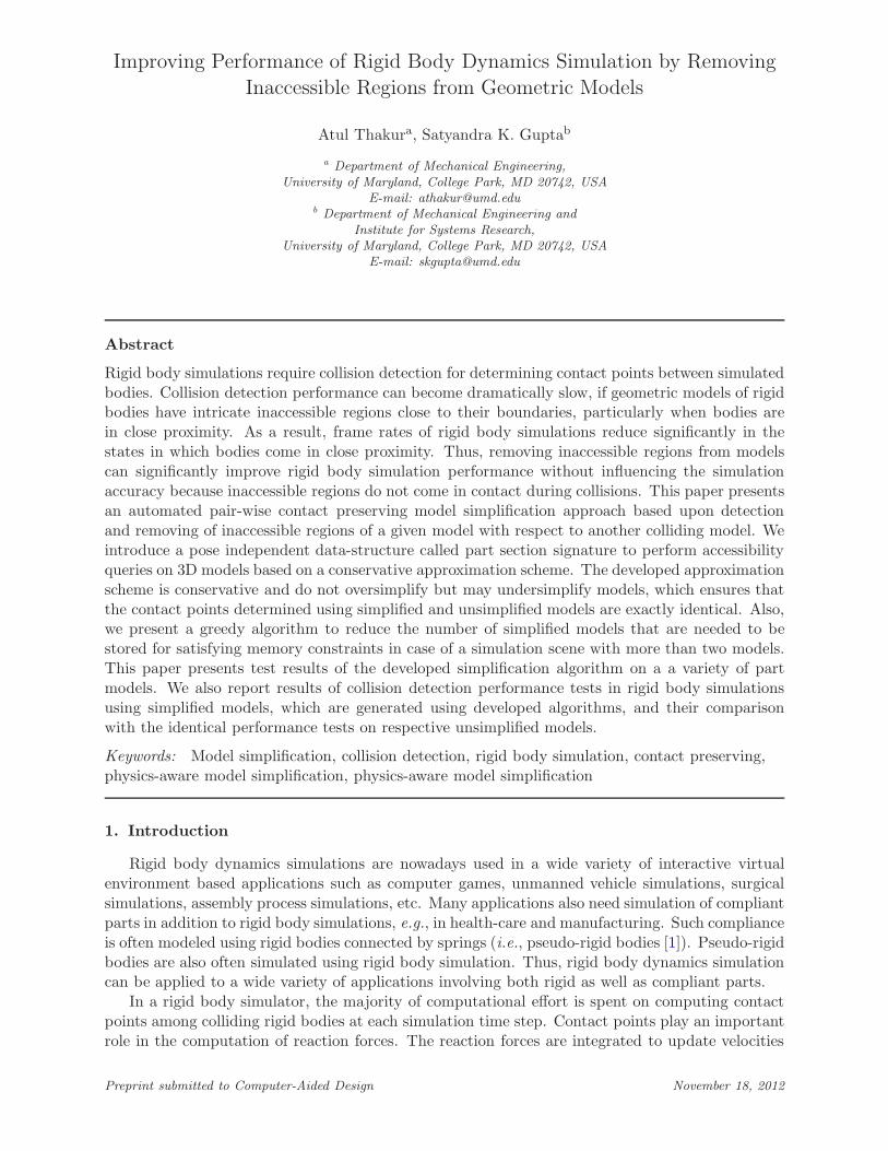
Figure 1: Collision computation time drastically increases when models are in close proximity.Collision detection search in hierarchical tree is deep due to inaccessible regions close to the surfaceof collision. Hierarchical decomposition does not prune the inaccessible facets of a model, whichcannot come in contact with other models (RAPID [2] collision detection engine was used for thistest).

3

(a) Vehicle assembly model.

Holes connecting

external and interior

regions

(b) Close up view of vehicle model to showholes connecting external and internal shellsprohibiting use of flood filling algorithm toeliminate interior inaccessible features.

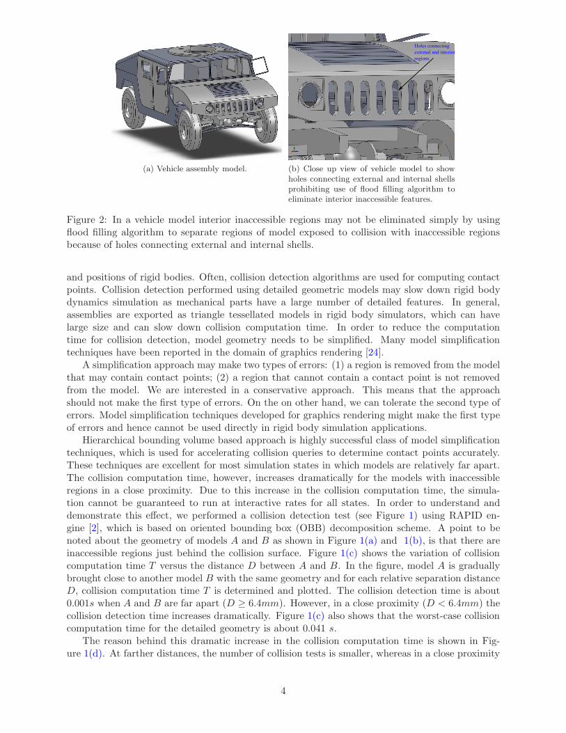
Figure 2: In a vehicle model interior inaccessible regions may not be eliminated simply by usingflood filling algorithm to separate regions of model exposed to collision with inaccessible regionsbecause of holes connecting external and internal shells.

and positions of rigid bodies. Often, collision detection algorithms are used for computing contactpoints. Collision detection performed using detailed geometric models may slow down rigid bodydynamics simulation as mechanical parts have a large number of detailed features. In general,assemblies are exported as triangle tessellated models in rigid body simulators, which can havelarge size and can slow down collision computation time. In order to reduce the computationtime for collision detection, model geometry needs to be simplified. Many model simplificationtechniques have been reported in the domain of graphics rendering [24].

A simplification approach may make two types of errors: (1) a region is removed from the modelthat may contain contact points; (2) a region that cannot contain a contact point is not removedfrom the model. We are interested in a conservative approach. This means that the approachshould not make the first type of errors. On the on other hand, we can tolerate the second type oferrors. Model simplification techniques developed for graphics rendering might make the first typeof errors and hence cannot be used directly in rigid body simulation applications.

Hierarchical bounding volume based approach is highly successful class of model simplificationtechniques, which is used for accelerating collision queries to determine contact points accurately.These techniques are excellent for most simulation states in which models are relatively far apart.The collision computation time, however, increases dramatically for the models with inaccessibleregions in a close proximity. Due to this increase in the collision computation time, the simula-tion cannot be guaranteed to run at interactive rates for all states. In order to understand anddemonstrate this effect, we performed a collision detection test (see Figure 1) using RAPID en-gine [2], which is based on oriented bounding box (OBB) decomposition scheme. A point to benoted about the geometry of models A and B as shown in Figure 1(a) and 1(b), is that there areinaccessible regions just behind the collision surface. Figure 1(c) shows the variation of collisioncomputation time T versus the distance D between A and B. In the figure, model A is graduallybrought close to another model B with the same geometry and for each relative separation distanceD, collision computation time T is determined and plotted. The collision detection time is about0.001s when A and B are far apart (D ≥ 6.4mm). However, in a close proximity (D < 6.4mm) thecollision detection time increases dramatically. Figure 1(c) also shows that the worst-case collisioncomputation time for the detailed geometry is about 0.041 s.

The reason behind this dramatic increase in the collision computation time is shown in Fig-ure 1(d). At farther distances, the number of collision tests is smaller, whereas in a close proximity

4

the number of collision tests increases. During the computations in the lowest level of the hierarchy,a large number of interior inaccessible facets, which are spatially very near to the point of collision,need to be tested. This causes considerable increase in the collision computation time when modelsare close. In many models similar to the one shown in Figure 2(a) (such as vehicles, boats, etc.),there are many details, which are inaccessible but spatially very close to the point of collision (seeFigure 2(b)). If inaccessible facets of a model are removed off-line (i.e., before the simulation) thenthis can reduce the computation time significantly without affecting the accuracy of the obtainedcontact points. We would like to note here that although the models described here are assemblies,we have exported them as tessellated models (in the form of STL files). This is required because, inthe existing rigid body simulators and collision detection engines, tessellated geometries (polygonsoup data as opposed to valid solid models) are used for contact point/force determination.

In some part models, the geometry is split into multiple shells. In such cases a simple floodfilling algorithm on the exterior shell can be used for separating interior and exterior shells and theninterior shells can be removed to generate simplified models. However, in many cases inaccessibleregions are located on the same shell (shown in Figure 2). In all the examples and case studiespresented in this paper, inaccessible regions lie on the same shell as the exterior regions. Hence,a simple flood filing algorithm does not work on such models and a more sophisticated modelsimplification approach for removing inaccessible regions is required for improving frame rates ofrigid body simulations.

The set of inaccessible facets depend upon the collision context (i.e., pair of models in collision).In many problems, the collision context is known in advance or can be easily determined as themodels in collision are known beforehand. This opens up a possibility of storing and retrievingmultiple simplified representations of models based on the corresponding collision contexts. Thisscheme is promising as the memory is relatively inexpensive compared to the real-time computa-tion of contact points for fully detailed models. We plan to utilize the collision context to generatecontact-preserving simplified models. This paper presents an accessibility based technique to sim-plify models with respect to each other in an off-line manner, i.e., before the simulation is performed,in such a way that the possible contact points are preserved. In order to perform a conservativepair-wise model simplification based on accessibility, we report a pose independent data structurecalled part section signature. We also report a greedy approach to reduce the number of pair-wisesimplified models to satisfy memory constraints for a given rigid body simulation scene with severalinteracting geometries.

In Section 2, we discuss some related work in the area of model simplification. Section 3,presents the problem statement and an overview of model simplification approach to solve theproblem. Section 4 to 6 discusses detailed description of the algorithms for model simplification.In Section 7 we discuss the implementation details and results and finally conclusions are presentedin Section 8.

2. Related work

Model simplification has been studied for various application domains such as interactive visualrendering, network transmission of models, finite element analysis, and collision detection. Ina previous paper, we classified the available model simplification techniques for physics basedsimulation applications based on the simplification operators into four types namely surface entitybased, volumetric entity based, explicit feature based and dimension reduction [3]. These categoriesare summarized below.

• Surface entity based techniques : In this approach, models are simplified by operating onsurface entities such as faces, edges and vertices. Under this category, reported techniquesare edge collapse technique [4], face clustering [5, 6] and low pass filtering approach such asFourier Transforms [7].

5

CAD models

Inaccessible

facets

Cross-section about XX

Model A Model B

Cross section about YY

Section YY

Inaccessible interior regions Inaccessible interior regions

Delete

inaccessible facets

Simplified model

Facets close to opening not deleted

Section XX

Simplified model

Facets close to opening not deleted

As Bs

Simplified

models

Find

inaccesible facets

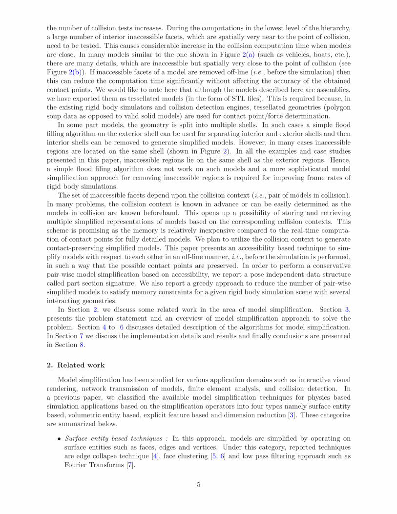
Figure 3: Contact preserving model simplification determines and removes inaccessible facets ofa model with respect to another model. Removal of inaccessible facets simplifies models whilepreserving potential contact points during collisions.

• Volumetric entity based techniques : In this approach, models are simplified by operatingon volumetric entities from the model. Major techniques reported under this category areeffective volume [8, 9, 10], cellular representation [11] and voxel [12, 13] based approaches.Boeing’s Voxmap PointShellTM uses voxel based representation for collision/proximity de-tection, swept volume generation, force modeling, spatial query, occlusion culling, real-timeshadows, and volume intersection applications [14].

• Explicit feature based techniques : Many reported model simplification techniques are basedon recognizing explicit application features prior to simplification. These techniques fallinto following categories: prismatic feature simplification, blend simplification, and arbitraryshaped feature simplification based on the type of features covered. In the explicit featurerepresentation based techniques, the feature information and semantics is explicitly extractedfrom the given CAD model or is present in the model in addition to the geometric and thetopological data. The features are user defined and depend on the context of application(e.g., in case of mechanical analysis, holes, slots, steps, pockets, fillets, rounds, etc. aresought features). Feature based modeling and feature recognition techniques are described indetails in [15].

6

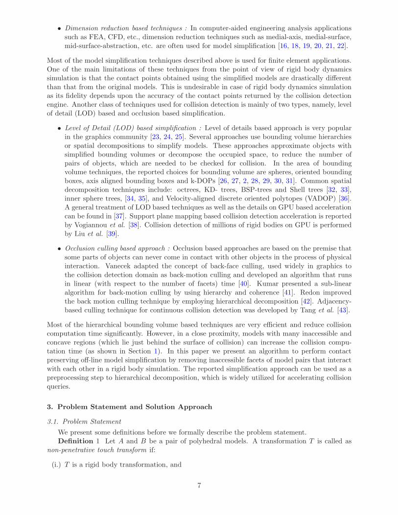
• Dimension reduction based techniques : In computer-aided engineering analysis applicationssuch as FEA, CFD, etc., dimension reduction techniques such as medial-axis, medial-surface,mid-surface-abstraction, etc. are often used for model simplification [16, 18, 19, 20, 21, 22].

Most of the model simplification techniques described above is used for finite element applications.One of the main limitations of these techniques from the point of view of rigid body dynamicssimulation is that the contact points obtained using the simplified models are drastically differentthan that from the original models. This is undesirable in case of rigid body dynamics simulationas its fidelity depends upon the accuracy of the contact points returned by the collision detectionengine. Another class of techniques used for collision detection is mainly of two types, namely, levelof detail (LOD) based and occlusion based simplification.

• Level of Detail (LOD) based simplification : Level of details based approach is very popularin the graphics community [23, 24, 25]. Several approaches use bounding volume hierarchiesor spatial decompositions to simplify models. These approaches approximate objects withsimplified bounding volumes or decompose the occupied space, to reduce the number ofpairs of objects, which are needed to be checked for collision. In the area of boundingvolume techniques, the reported choices for bounding volume are spheres, oriented boundingboxes, axis aligned bounding boxes and k-DOPs [26, 27, 2, 28, 29, 30, 31]. Common spatialdecomposition techniques include: octrees, KD- trees, BSP-trees and Shell trees [32, 33],inner sphere trees, [34, 35], and Velocity-aligned discrete oriented polytopes (VADOP) [36].A general treatment of LOD based techniques as well as the details on GPU based accelerationcan be found in [37]. Support plane mapping based collision detection acceleration is reportedby Vogiannou et al. [38]. Collision detection of millions of rigid bodies on GPU is performedby Liu et al. [39].

• Occlusion culling based approach : Occlusion based approaches are based on the premise thatsome parts of objects can never come in contact with other objects in the process of physicalinteraction. Vanecek adapted the concept of back-face culling, used widely in graphics tothe collision detection domain as back-motion culling and developed an algorithm that runsin linear (with respect to the number of facets) time [40]. Kumar presented a sub-linearalgorithm for back-motion culling by using hierarchy and coherence [41]. Redon improvedthe back motion culling technique by employing hierarchical decomposition [42]. Adjacency-based culling technique for continuous collision detection was developed by Tang et al. [43].

Most of the hierarchical bounding volume based techniques are very efficient and reduce collisioncomputation time significantly. However, in a close proximity, models with many inaccessible andconcave regions (which lie just behind the surface of collision) can increase the collision compu-tation time (as shown in Section 1). In this paper we present an algorithm to perform contactpreserving off-line model simplification by removing inaccessible facets of model pairs that interactwith each other in a rigid body simulation. The reported simplification approach can be used as apreprocessing step to hierarchical decomposition, which is widely utilized for accelerating collisionqueries.

3. Problem Statement and Solution Approach

3.1. Problem Statement

We present some definitions before we formally describe the problem statement.Definition 1 Let A and B be a pair of polyhedral models. A transformation T is called as

non-penetrative touch transform if:

(i.) T is a rigid body transformation, and

7

(ii.) touch(A,TB) = true and penetration(A,TB) = false

where,

touch(X,Y ) =

true, int(X) ∩ int(Y ) = φ and bnd(X) ∩ bnd(Y ) 6= φfalse, otherwise

(1)

and,

penetration(X,Y ) =

true, int(X) ∩ int(Y ) 6= φfalse, otherwise

(2)

int(.) is the interior of the point set, bnd(.) is the boundary of the point set and φ is the null set. Itshould be noted that we do not directly compute the touch and penetration based on the definitionspresented here. These terms are introduced in order to explain the inaccessibility of facets, whichare computed in subsequent sections.

Definition 2 Let A and B be a pair of polyhedral models. We define a set of inaccessible facetsof A with respect to B as Ain,B ⊂ A such that for all possible non-penetrative touch transforms T ,Ain,B ∩ TB = φ.

Problem Statement : Given a pair of models A and B, generate simplified models As andBs such that, the set of contact points obtained under every non-penetrative touch transform of Arelative to B and As relative to Bs is the same. This can be mathematically expressed as following.Let CA,B = A ∩ TB and CAs,Bs

= As ∩ TBs, where T be a non-penetrative touch transformation.We want to generate simplified models As and Bs, such that CA,B = CAs,Bs

. Here, As = A−Ain,B

and Bs = B −Bin,A.In this paper we represent all the example models (including assemblies) using triangle tessel-

lated models. This approximation is valid as in most of the publicly available rigid body simulatorsthe input model requirement is triangular tessellation.

3.2. Overview of the Approach

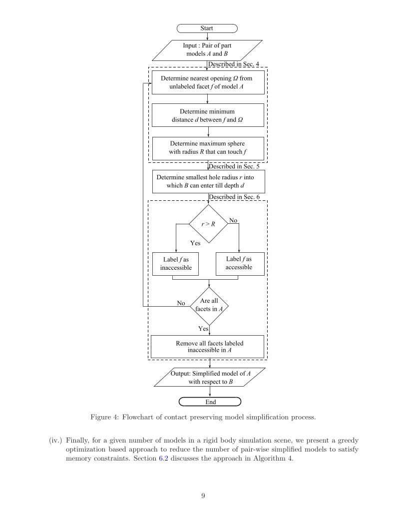
The overall model simplification approach is depicted in the form of a flowchart in Figure 4 andindividual computational steps are described below.

(i.) In order to make contact with any facet f on the concave portion of A, model B will needto access facet f via some passage or opening on A (described in Section 4 and Figure 5(b)and 6(b)). These passages and openings impose restrictions on the size of B that can reachf (e.g., if B is very large compared to the available passage and opening, then it cannotreach f). Section 4 presents a formal approach in Algorithm 1 to automatically identify andrepresent concave regions, openings, and passages.

(ii.) We are interested in knowing how deep B can enter into a passage of A. Usually partswith large cross-section with respect to a passage can only enter the passage up to a certaindistance before the cross-section becomes the bottleneck. Parts have different cross-sectionsin different directions. Hence, in order to figure out if a part can enter an opening or passage,we need pose independent measure of its size along its length. Computing this informationexactly is not practical. So we have developed method to compute a conservative estimate ofthis key information. We refer to this measure as part section signature. Section 5 describesAlgorithm 2 for computing the part section signature.

(iii.) For a given passage on A and part section signature of B, we analyze if B is small enough toenter a passage of A and reach f or not. Facets on the concave portions of A that cannot bereached by B due to the large size of B with respect to the available passages and openings onA can be removed during the contact determination step. Section 6.1 describes Algorithm 3to determine and remove the list of inaccessible regions of the model with respect to anothermodel for a given model pair to obtain simplified models.

8

Input : Pair of part

models A and B

Determine nearest opening Ω from

unlabeled facet f of model A

Determine minimum

distance d between f and Ω

Determine maximum sphere

with radius R that can touch f

Determine smallest hole radius r into

which B can enter till depth d

r > R

Label f as

inaccessible

Yes

Are all

facets in A

Label f as

accessible

No

Remove all facets labeled inaccessible in A

Yes

No

Output: Simplified model of A

with respect to B

Start

End

Described in Sec. 4

Described in Sec. 5

Described in Sec. 6

Figure 4: Flowchart of contact preserving model simplification process.

(iv.) Finally, for a given number of models in a rigid body simulation scene, we present a greedyoptimization based approach to reduce the number of pair-wise simplified models to satisfymemory constraints. Section 6.2 discusses the approach in Algorithm 4.

9

(a) 3D CAD model for A.

Passage 1

Passage 2

(b) Passages of A.

(c) 2D cross-section view of A.

Figure 5: 3D CAD model and passage set (passages of A are obtained by subtracting the A fromthe convex hull of A). Passages denote regions in space through which facets of a model are touchedby another model without penetration.

4. Determining Passages

We first define the notion of passages, deep facets, and openings and then present our approachto determine them for a given model.

Definition 3 We define a passage set P for a given model A as the set of 3D point sets pA,i,such that, all points in pA,i belongs to the interior of the convex hull of A but do not belong to the

10

Deep facets associated with Passage 1

Deep facets associated with Passage 2

(a) Deep facets of A corresponding to each passageshown in Figure 5.

Openings assosciated with Passage 2

Openings assosciated with Passage 1

(b) Openings of A corresponding to each passageshown in Figure 5.

Figure 6: Deep facets and openings of A.

interior of A.P (A) = Ac −A (3)

where, P (A) is the passage set of model A and Ac is the convex hull of model A. Also, P (A) = ∪pA,i

and pA,m ∩ pA,n = φ for all m 6= n, where, each pA,m represents a mutually exclusive passage ofA. The passage set of the model shown in Figure 5(a) are illustrated in Figure 5(b). There areonly two passages because of the presence of a hole, which connects the inner and outer shell (seeFigure 5(c)).

Definition 4 A deep facet FD of a model is defined as a set points pi satisfying, pi ∈ int(Ac)and pi ∈ bnd(A), ∀pi ∈ FD.

The deep facets of the model shown in Figure 5(a) are illustrated in Figure 6(a).In other words, deep facets of a model are those bounding facets of the model that strictly lies

in the interior of the convex hull of the model.Definition 5 An opening Ω of model A is a set of points satisfying following:

(i.) Ω is a connected set, and

(ii.) pi ∈ bnd(Ac) and pi /∈ bnd(A), ∀pi ∈ Ω.

In other words, an opening of a model A is a connected virtual face that bounds a passage andstrictly lies on the boundary of convex hull of A but does not lie on the boundary of A. Openingsare actually computed by determining the tessellation (triangular facets) of the virtual face whichlies on the convex hull of the model but not on the model itself and the procedure for the same isexplained in this section in step 2. Openings of model A are shown in Figure 6(b).

Definition 6 An opening Ω and a deep facet FD are said to be connected if they lie on thesame passage pA,i.

Definition 7 Opening distance of a deep facet FD connected to openings Ωj belonging to apassage pA,i is the length of a line segment between a pair of points pm ∈ Ωj and pn ∈ FD, suchthat the line segment L connecting pm and pn satisfies following two conditions, namely,

11

(i.) all points on L connecting pi and pj strictly lies inside the volume of the cell pA,i, and

(ii.) L does not intersect any deep facet belonging to pA,i.

If a line segment L satisfying above two conditions does not exist then opening distance is equalto infinity.

The largest sphere that can be inscribed inside the volume of pA,i and is tangential to FD iscalled as opening sphere and the radius of the opening sphere is called as opening radius.

Some deep facets of A lying on pA,i may not be connected to any opening. In case of such anorphan deep facet, the opening distance is set as infinity. Opening sphere is determined for suchorphan facets by finding out the largest non-intersecting inscribed sphere inside the passage pA,i

and tangential to the deep facet.Thus, each deep facet can have multiple (at least one) opening distances and corresponding to

each connected opening there is an associated opening sphere.Another interpretation of opening sphere is that for a given opening of a deep facet, any sphere

with radius larger than the opening sphere cannot touch the deep facet without penetration.Following steps are used to determine passage set, deep facets, and openings of a given model

and to represent the model as a graph whose nodes contain deep facets and openings while arcsrepresent the connectivity information.

Algorithm 1 - Construct Connectivity Graph

Input - Polyhedral model A.

Output - Connectivity graph representation of A.

Steps:

(i.) Find the passage set A : Determine the convex hull Ac of model A and perform the Booleansubtraction of Ac and A. This results into a non-manifold passage set P (A). The passageset of the model shown in Figure 5(a) is shown in Figure 5(b). We express A and Ac asNef-polyhedrons as implemented in CGAL [44, 45].

(ii.) Find openings of A : Iterate through each bounding facet of passages pA,i of P (A). Labelevery facet in pA,i, that do not lie on bounding facets of A but do lie on bounding facetsof Ac as opening facets. Group all contiguous facets marked as opening facets and storeas the sets of openings corresponding to the passage pA,i. We used CGAL’s AABB spatialsearch structure to accelerate this process [44]. Openings of the model shown in Figure 5(a)is depicted in Figure 6(b).

(iii.) Find deep facets of A : Iterate through bounding facets of model A and find all facets ofA that are coincident with bounding facets (that are not openings) of the passage pA,i, andlabel them as deep facets.

(iv.) Construct a connectivity graph for each passage pA,i : Construct a connectivity graph forpA,i and mark each node either as opening or deep as determined in steps (ii) and (iii).Determine connected opening nodes for each deep node and add to the connectivity graph.A node of the graph represents either a deep facet or an opening while an arc represents theconnectivity between nodes. Iterate through nodes representing deep facets and determinethe bounding sphere for each connected opening and store it as the opening sphere of theconnected deep facets. This is because bounding sphere of an opening is always larger thanor equal to the opening sphere and we need an upper bound on the opening sphere radius.Compute the minimum distance between the deep facet and connected openings and storeas opening distance for the deep facet. If some deep facet is not connected to any opening

12

Range

R

Last Supporting

Plane

Slicing

Plane

First Supporting

Plane

Cross-section

PF

PL

PS

d

D

(a) Supporting planes and range along direc-

tion vector ~d.

Minimum

Cylinder CM

D

d

Cross-section

Slicing

Plane PS

First

Supporting

Plane PF

(b) Minimum cylinder along direction vector~d and for depth D.

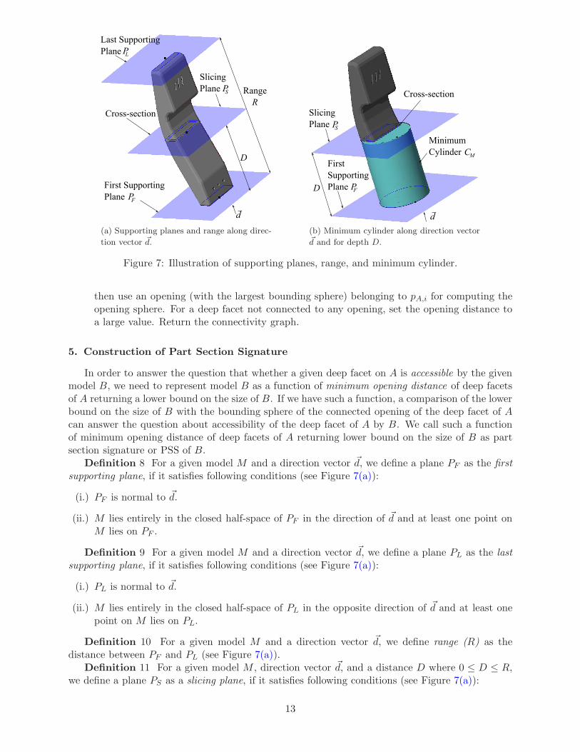
Figure 7: Illustration of supporting planes, range, and minimum cylinder.

then use an opening (with the largest bounding sphere) belonging to pA,i for computing theopening sphere. For a deep facet not connected to any opening, set the opening distance toa large value. Return the connectivity graph.

5. Construction of Part Section Signature

In order to answer the question that whether a given deep facet on A is accessible by the givenmodel B, we need to represent model B as a function of minimum opening distance of deep facetsof A returning a lower bound on the size of B. If we have such a function, a comparison of the lowerbound on the size of B with the bounding sphere of the connected opening of the deep facet of Acan answer the question about accessibility of the deep facet of A by B. We call such a functionof minimum opening distance of deep facets of A returning lower bound on the size of B as partsection signature or PSS of B.

Definition 8 For a given model M and a direction vector ~d, we define a plane PF as the firstsupporting plane, if it satisfies following conditions (see Figure 7(a)):

(i.) PF is normal to ~d.

(ii.) M lies entirely in the closed half-space of PF in the direction of ~d and at least one point onM lies on PF .

Definition 9 For a given model M and a direction vector ~d, we define a plane PL as the lastsupporting plane, if it satisfies following conditions (see Figure 7(a)):

(i.) PL is normal to ~d.

(ii.) M lies entirely in the closed half-space of PL in the opposite direction of ~d and at least onepoint on M lies on PL.

Definition 10 For a given model M and a direction vector ~d, we define range (R) as thedistance between PF and PL (see Figure 7(a)).

Definition 11 For a given model M , direction vector ~d, and a distance D where 0 ≤ D ≤ R,we define a plane PS as a slicing plane, if it satisfies following conditions (see Figure 7(a)):

13

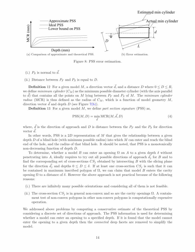
(a) Comparison of approximate and theoretical PSS. (b) Error estimation.

Figure 8: PSS error estimation.

(i.) PS is normal to ~d.

(ii.) Distance between PF and PS is equal to D.

Definition 12 For a given model M , a direction vector ~d, and a distance D where 0 ≤ D ≤ R,we defineminimum cylinder (CM ) as the minimum possible diameter cylinder (with the axis parallelto ~d) that contains all the points on M lying between PF and PS of M . The minimum cylinderradius (MCR) is thus defined as the radius of CM , which is a function of model geometry M ,direction vector ~d and depth D (see Figure 7(b)).

Definition 13 For a given model M , we define part section signature (PSS) as,

PSS(M,D) = min~d

MCR(M, ~d,D) (4)

where, ~d is the direction of approach and D is distance between the PF and the PS for directionvector ~d.

In other words, PSS is a 2D representation of M that gives the relationship between a givendepth D of a blind hole (with minimum possible radius) into whichM can enter and reach the blindend of the hole, and the radius of that blind hole. It should be noted, that PSS is a monotonicallynon-decreasing function of depth D.

To determine, whether a model B can enter an opening Ω on A to a given depth δ withoutpenetrating into A, ideally requires to try out all possible directions of approach ~dj for B and tofind the corresponding set of cross-sections CSj obtained by intersecting B with the slicing plane

for the direction ~dj and depths 0 ≤ D ≤ δ. If at least one cross-section CSj is such that it canbe contained in maximum inscribed polygon of Ω, we can claim that model B enters the cavityopening Ω to a distance of δ. However the above approach is not practical because of the followingreasons:

(i.) There are infinitely many possible orientations and considering all of them is not feasible.

(ii.) The cross-section CSj is in general non-convex and so are the cavity openings Ω. A contain-ment test of non-convex polygons in other non-convex polygons is computationally expensiveoperation.

We addressed above problems by computing a conservative estimate of the theoretical PSS byconsidering a discrete set of directions of approach. The PSS information is used for determiningwhether a model can enter an opening to a specified depth. If it is found that the model cannotenter the opening to a given depth then the connected deep facets are removed to simplify themodel.

14

We are interested in conservative simplification (i.e., we do not want to change contact pointsdue to approximations in PSS). Hence, we computed a lower bound on the theoretical PSS andused it as a conservative estimate of the theoretical PSS. The approximated, theoretical, and theestimated lower bound on the PSS is shown schematically in Figure 8(a). The estimated lowerbound on PSS of a model guarantees that the model cannot enter a given hole if the theoreticalPSS of the model does not do so. This approach ensures that a facet is deleted only when it istruly inaccessible. However, sometimes a facet may be inaccessible but our approach will not beable to eliminate that due to the use of the estimated lower bound on the PSS.

In our approach, we determine a discrete set of directions along (θ, φ) in spherical coordinatesystem with θ = α, 2α, ...., 2π radians and φ = α, 2α, ...., 2π radians, where α is the angular incre-ment. For each direction, we determine MCR at various depths and then find out an approximatePSS. To estimate how much the actual PSS can be less than the computed approximate PSS,consider Figure 8(b). The ideal cylinder (with diameter d) enveloping a model to a depth of l isshown by a rectangle drawn in solid line in Figure 8(b). The estimated minimum cylinder (withdiameter D) enveloping the model is shown by a broken line in Figure 8(b), whose axis is at anangle of ψ ≤ α with the axis of ideal minimum cylinder. Now, using the geometry,

dcos(ψ) + lsin(ψ) = D ⇒ dD

= sec(ψ) − lDtan(ψ),

∵ ψ is very small and expressed in radians, sec(ψ) ≈ 1 and tan(ψ) ≈ sin(ψ) ≈ ψ,

⇒ dD

≈ 1− lDψ, ⇒ d

D= 1− l

Dψ ≥ 1− l

Dα, ∵ ψ ≤ α,

thus,

d ≥ D1−l

Dα (5)

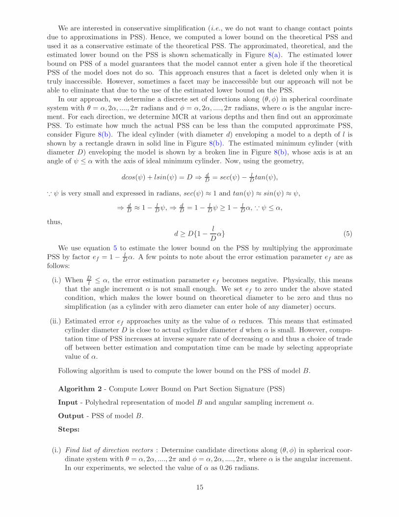
We use equation 5 to estimate the lower bound on the PSS by multiplying the approximatePSS by factor ef = 1 − l

Dα. A few points to note about the error estimation parameter ef are as

follows:

(i.) When Dl≤ α, the error estimation parameter ef becomes negative. Physically, this means

that the angle increment α is not small enough. We set ef to zero under the above statedcondition, which makes the lower bound on theoretical diameter to be zero and thus nosimplification (as a cylinder with zero diameter can enter hole of any diameter) occurs.

(ii.) Estimated error ef approaches unity as the value of α reduces. This means that estimatedcylinder diameter D is close to actual cylinder diameter d when α is small. However, compu-tation time of PSS increases at inverse square rate of decreasing α and thus a choice of tradeoff between better estimation and computation time can be made by selecting appropriatevalue of α.

Following algorithm is used to compute the lower bound on the PSS of model B.

Algorithm 2 - Compute Lower Bound on Part Section Signature (PSS)

Input - Polyhedral representation of model B and angular sampling increment α.

Output - PSS of model B.

Steps:

(i.) Find list of direction vectors : Determine candidate directions along (θ, φ) in spherical coor-dinate system with θ = α, 2α, ...., 2π and φ = α, 2α, ...., 2π, where α is the angular increment.In our experiments, we selected the value of α as 0.26 radians.

15

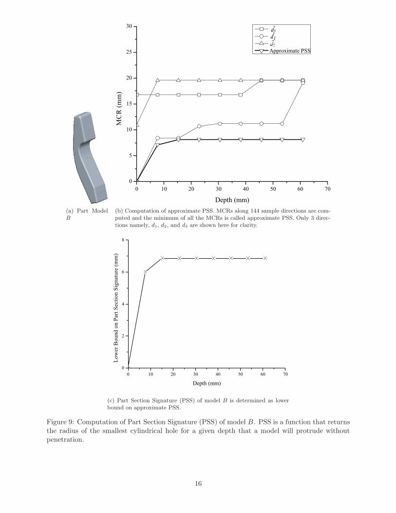
(a) Part ModelB

0 10 20 30 40 50 60 700

5

10

15

20

25

30

MC

R (m

m)

Depth (mm)

Approximate PSS

(b) Computation of approximate PSS. MCRs along 144 sample directions are com-puted and the minimum of all the MCRs is called approximate PSS. Only 3 direc-tions namely, d1, d2, and d3 are shown here for clarity.

0 10 20 30 40 50 60 700

2

4

6

8

Low

er B

ound

on

Part

Sect

ion

Sign

atur

e (m

m)

Depth (mm)

(c) Part Section Signature (PSS) of model B is determined as lowerbound on approximate PSS.

Figure 9: Computation of Part Section Signature (PSS) of model B. PSS is a function that returnsthe radius of the smallest cylindrical hole for a given depth that a model will protrude withoutpenetration.

16

(ii.) Find the slicing plane set along each direction vector : Find the first supporting plane, lastsupporting plane and range along each candidate direction. After this, generate slicing planesnormal to the direction vector and add to the slicing plane set using the list of depths of deepfacets on A. If the depth for a direction is larger than the range in that direction then thedepth is set equal to the range.

(iii.) Compute cross-sections along each direction vector : Intersect the model with each plane inthe slicing plane set to obtain the point set lying in the negative half space of the intersectingplane. After this, determine the MCR of each point set. In order to eliminate redundantcomputations, only compute cross-sections for the range of depths of deep facets obtained inAlgorithm 1. For each candidate direction, store the MCR variation along it. Figure 9(b)shows the variation of MCR along three directions (~d1, ~d2, and ~d3) for the model B.

(iv.) Compute approximate PSS : Determine MCR for each direction determined in step (i.). Afterthis, for each direction, find out the minimum among all MCRs corresponding to each intervaland generate a lookup table for each direction storing the depth and the minimum MCR. Thislookup table is called the approximate PSS. In Figure 9(b) only three representative directions~d1, ~d2 and ~d3 are shown for clarity.

(v.) Apply conservative bound on the approximate PSS : Multiply factor ef given in Equation 5to approximate PSS and determine the lower bound on the PSS. The estimated lower boundon the PSS is shown in Figure 9(c). Return estimated PSS of the model B.

6. Model Simplification

In this section we describe model simplification algorithms based on data-structure developedin Sections 4 and 5.

6.1. Pair-Wise Model Simplification

Each deep facet of the connectivity graph of passages of model A is traversed to find out theiraccessibility through their corresponding connected openings using the PSS of the model B. Theinaccessible deep facets of A with respect to B are subsequently deleted to generate the simplifiedmodel As. Steps followed for pair-wise simplification are listed in Algorithm 3.

Algorithm 3 - Perform Pair-Wise Model Simplification

Input - Connectivity graph representation of models A and B and PSS of models A and B.

Output - Simplified models As and Bs.

Steps:

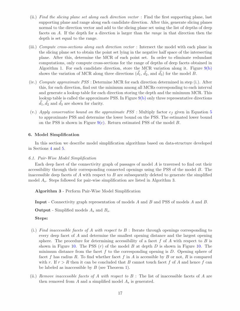
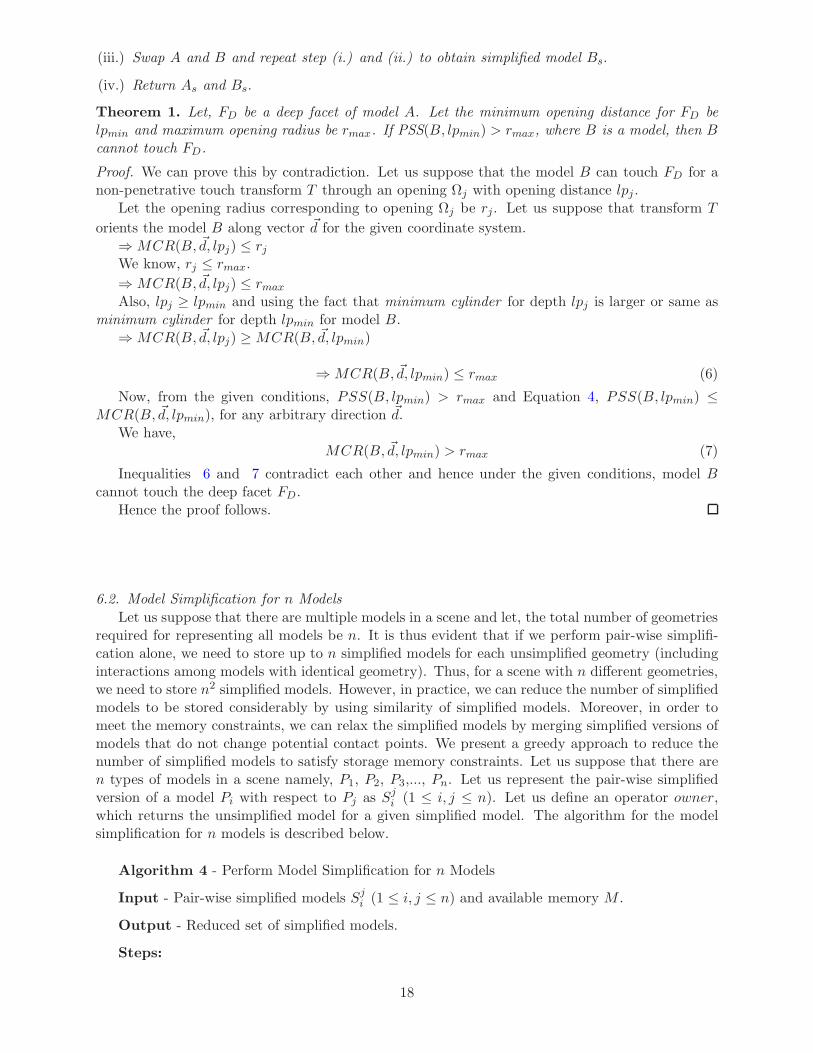
(i.) Find inaccessible facets of A with respect to B : Iterate through openings corresponding toevery deep facet of A and determine the smallest opening distance and the largest openingsphere. The procedure for determining accessibility of a facet f of A with respect to B isshown in Figure 10. The PSS (r) of the model B at depth D is shown in Figure 10. Theminimum distance from the facet f to the corresponding opening is D. Opening sphere offacet f has radius R. To find whether facet f in A is accessible by B or not, R is comparedwith r. If r > R then it can be concluded that B cannot touch facet f of A and hence f canbe labeled as inaccessible by B (see Theorem 1).

(ii.) Remove inaccessible facets of A with respect to B : The list of inaccessible facets of A arethen removed from A and a simplified model As is generated.

17

(iii.) Swap A and B and repeat step (i.) and (ii.) to obtain simplified model Bs.

(iv.) Return As and Bs.

Theorem 1. Let, FD be a deep facet of model A. Let the minimum opening distance for FD belpmin and maximum opening radius be rmax. If PSS(B, lpmin) > rmax, where B is a model, then Bcannot touch FD.

Proof. We can prove this by contradiction. Let us suppose that the model B can touch FD for anon-penetrative touch transform T through an opening Ωj with opening distance lpj .

Let the opening radius corresponding to opening Ωj be rj. Let us suppose that transform T

orients the model B along vector ~d for the given coordinate system.⇒MCR(B, ~d, lpj) ≤ rjWe know, rj ≤ rmax.

⇒MCR(B, ~d, lpj) ≤ rmax

Also, lpj ≥ lpmin and using the fact that minimum cylinder for depth lpj is larger or same asminimum cylinder for depth lpmin for model B.

⇒MCR(B, ~d, lpj) ≥MCR(B, ~d, lpmin)

⇒MCR(B, ~d, lpmin) ≤ rmax (6)

Now, from the given conditions, PSS(B, lpmin) > rmax and Equation 4, PSS(B, lpmin) ≤MCR(B, ~d, lpmin), for any arbitrary direction ~d.

We have,MCR(B, ~d, lpmin) > rmax (7)

Inequalities 6 and 7 contradict each other and hence under the given conditions, model Bcannot touch the deep facet FD.

Hence the proof follows.

6.2. Model Simplification for n Models

Let us suppose that there are multiple models in a scene and let, the total number of geometriesrequired for representing all models be n. It is thus evident that if we perform pair-wise simplifi-cation alone, we need to store up to n simplified models for each unsimplified geometry (includinginteractions among models with identical geometry). Thus, for a scene with n different geometries,we need to store n2 simplified models. However, in practice, we can reduce the number of simplifiedmodels to be stored considerably by using similarity of simplified models. Moreover, in order tomeet the memory constraints, we can relax the simplified models by merging simplified versions ofmodels that do not change potential contact points. We present a greedy approach to reduce thenumber of simplified models to satisfy storage memory constraints. Let us suppose that there aren types of models in a scene namely, P1, P2, P3,..., Pn. Let us represent the pair-wise simplifiedversion of a model Pi with respect to Pj as Sj

i (1 ≤ i, j ≤ n). Let us define an operator owner,which returns the unsimplified model for a given simplified model. The algorithm for the modelsimplification for n models is described below.

Algorithm 4 - Perform Model Simplification for n Models

Input - Pair-wise simplified models Sji (1 ≤ i, j ≤ n) and available memory M .

Output - Reduced set of simplified models.

Steps:

18

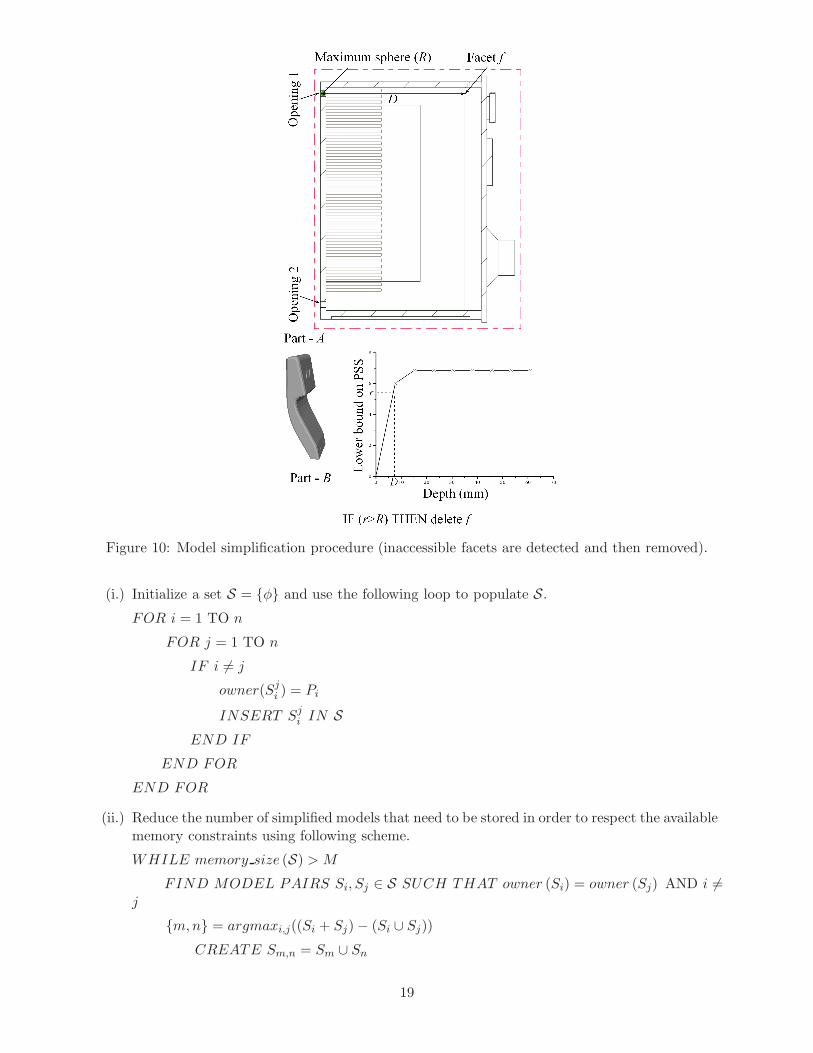
Figure 10: Model simplification procedure (inaccessible facets are detected and then removed).

(i.) Initialize a set S = φ and use the following loop to populate S.

FOR i = 1 TO n

FOR j = 1 TO n

IF i 6= j

owner(Sji ) = Pi

INSERT Sji IN S

END IF

END FOR

END FOR

(ii.) Reduce the number of simplified models that need to be stored in order to respect the availablememory constraints using following scheme.

WHILE memory size (S) > M

FIND MODEL PAIRS Si, Sj ∈ S SUCH THAT owner (Si) = owner (Sj) AND i 6=j

m,n = argmaxi,j((Si + Sj)− (Si ∪ Sj))

CREATE Sm,n = Sm ∪ Sn

19

(a) Intruder blocking mission. (b) Screen-shot of the virtual environment.

Figure 11: USV intruder blocking game.

owner (Sm,n) = owner (Sm)

REMOV E Sm AND Sn FROM S

INSERT Sm,n IN S

END IF

END WHILE

(iii.) Return reduced set S.

In the above algorithm, each pair of simplified versions of a model is tested for uncommon facets.The simplified model pair of same owner, which has the largest number of uncommon facets, isfused to generate a relaxed simplified model. This process is repeated until, number of simplifiedversions of model satisfy the storage memory constraint.

7. Implementation and Results

We developed a prototype software implementation of the contact preserving model simplifica-tion algorithm discussed in this paper. The programming platform was chosen as VC++ (version8) using CGAL 3.6 on Windows Vista operating system [44]. Our implementation takes STL filesas input and after simplification, generates output in the same format. Also, we represent assemblymodels in stl format. In this section we present some results of model simplification approach devel-oped in this paper, mainly in two robotics applications, namely, unmanned surface vehicle (USV)simulation and ground vehicle simulation. We also present some more examples to demonstratethe utility of the technique developed in this paper.

We have been developing a virtual environment to simulate surveillance operation for USVs[46, 47], in which we used the simplified models generated using the approach discussed in thispaper. The virtual environment simulates a maritime mission in which a remote controlled boattries to protect a valuable target from an intruding boat. Figure 11(a) shows the schematic viewof the mission, where the intruder boat attempts to reach to the protected object by crossing thebuffer zone and the danger zone. The USV’s task is to block the intruder. The level of aggression,with which the USV blocks the intruder depends upon the position of the intruder (i.e., whether theintruder lies in the buffer zone or the danger zone). The USV should block the intruder and at thesame time should avoid collision with the other dynamic obstacles, which represent the harmless

20

Section XX

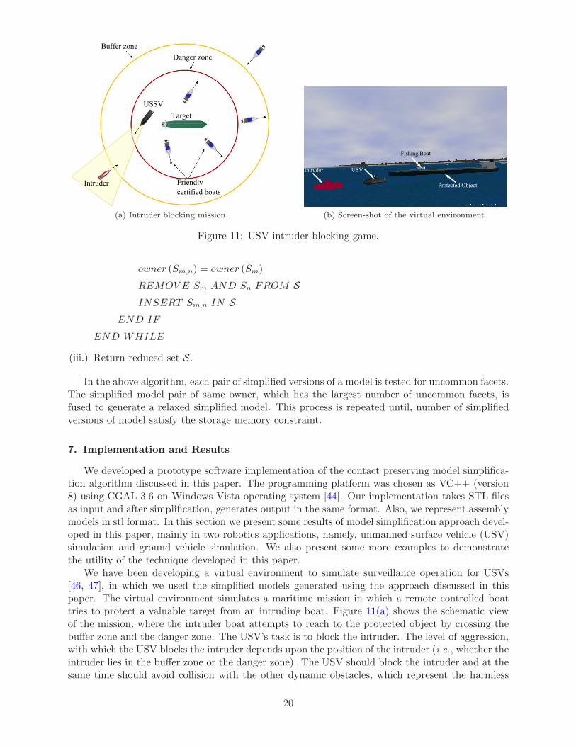
(a) USV model with 60030facets.

(b) Cut-through view (aboutplane XX) of unsimplified USVmodel with 60030 facets.

(c) Cut-through view (aboutplane XX) of simplified USVmodel with 1120 facets.

Figure 12: Boat model used in the virtual environment.

0 5 10 15 20 25 30

0.00

0.05

0.10

0.15

0.20

0.25

0.30

Col

lisio

n co

mpu

tatio

n tim

e (s

)

Distance between boats (mm)

Collision computation time for unsimplified boat model (s) Collision computation time for simplified boat model (s)

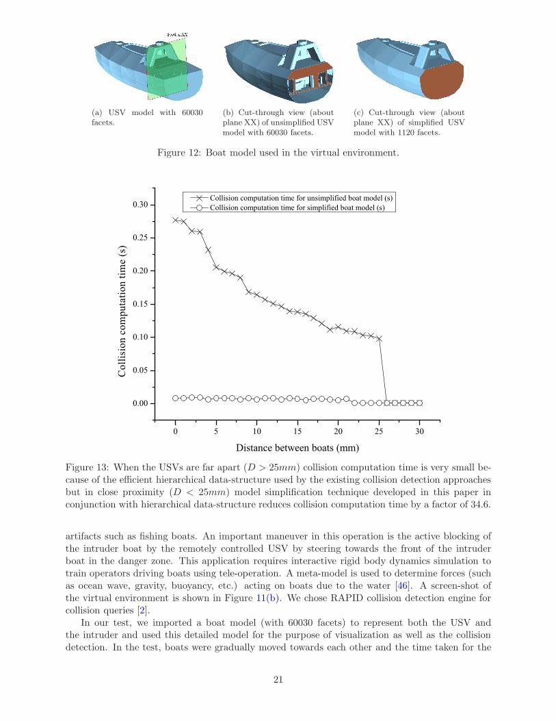
Figure 13: When the USVs are far apart (D > 25mm) collision computation time is very small be-cause of the efficient hierarchical data-structure used by the existing collision detection approachesbut in close proximity (D < 25mm) model simplification technique developed in this paper inconjunction with hierarchical data-structure reduces collision computation time by a factor of 34.6.

artifacts such as fishing boats. An important maneuver in this operation is the active blocking ofthe intruder boat by the remotely controlled USV by steering towards the front of the intruderboat in the danger zone. This application requires interactive rigid body dynamics simulation totrain operators driving boats using tele-operation. A meta-model is used to determine forces (suchas ocean wave, gravity, buoyancy, etc.) acting on boats due to the water [46]. A screen-shot ofthe virtual environment is shown in Figure 11(b). We chose RAPID collision detection engine forcollision queries [2].

In our test, we imported a boat model (with 60030 facets) to represent both the USV andthe intruder and used this detailed model for the purpose of visualization as well as the collisiondetection. In the test, boats were gradually moved towards each other and the time taken for the

21

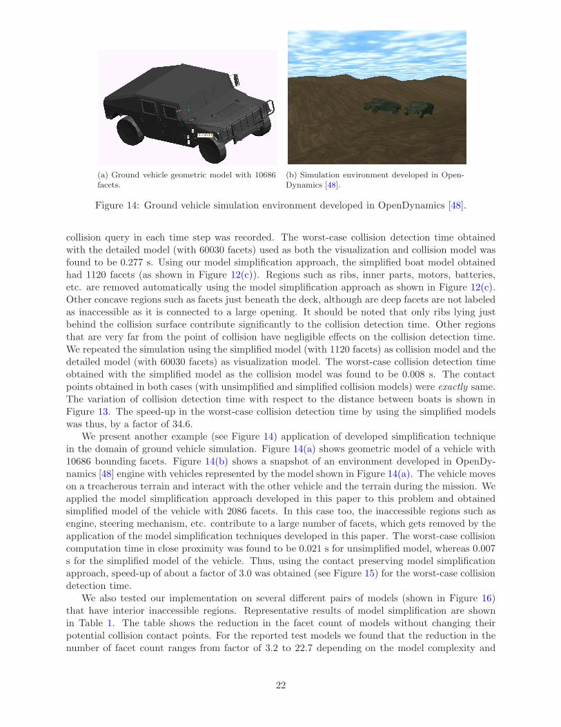
(a) Ground vehicle geometric model with 10686facets.

(b) Simulation environment developed in Open-Dynamics [48].

Figure 14: Ground vehicle simulation environment developed in OpenDynamics [48].

collision query in each time step was recorded. The worst-case collision detection time obtainedwith the detailed model (with 60030 facets) used as both the visualization and collision model wasfound to be 0.277 s. Using our model simplification approach, the simplified boat model obtainedhad 1120 facets (as shown in Figure 12(c)). Regions such as ribs, inner parts, motors, batteries,etc. are removed automatically using the model simplification approach as shown in Figure 12(c).Other concave regions such as facets just beneath the deck, although are deep facets are not labeledas inaccessible as it is connected to a large opening. It should be noted that only ribs lying justbehind the collision surface contribute significantly to the collision detection time. Other regionsthat are very far from the point of collision have negligible effects on the collision detection time.We repeated the simulation using the simplified model (with 1120 facets) as collision model and thedetailed model (with 60030 facets) as visualization model. The worst-case collision detection timeobtained with the simplified model as the collision model was found to be 0.008 s. The contactpoints obtained in both cases (with unsimplified and simplified collision models) were exactly same.The variation of collision detection time with respect to the distance between boats is shown inFigure 13. The speed-up in the worst-case collision detection time by using the simplified modelswas thus, by a factor of 34.6.

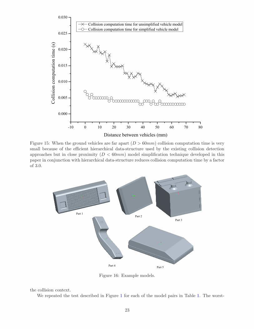
We present another example (see Figure 14) application of developed simplification techniquein the domain of ground vehicle simulation. Figure 14(a) shows geometric model of a vehicle with10686 bounding facets. Figure 14(b) shows a snapshot of an environment developed in OpenDy-namics [48] engine with vehicles represented by the model shown in Figure 14(a). The vehicle moveson a treacherous terrain and interact with the other vehicle and the terrain during the mission. Weapplied the model simplification approach developed in this paper to this problem and obtainedsimplified model of the vehicle with 2086 facets. In this case too, the inaccessible regions such asengine, steering mechanism, etc. contribute to a large number of facets, which gets removed by theapplication of the model simplification techniques developed in this paper. The worst-case collisioncomputation time in close proximity was found to be 0.021 s for unsimplified model, whereas 0.007s for the simplified model of the vehicle. Thus, using the contact preserving model simplificationapproach, speed-up of about a factor of 3.0 was obtained (see Figure 15) for the worst-case collisiondetection time.

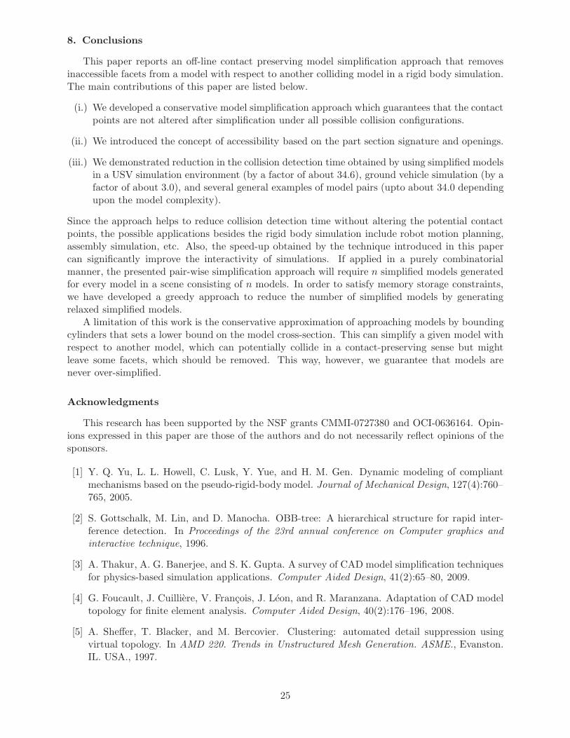
We also tested our implementation on several different pairs of models (shown in Figure 16)that have interior inaccessible regions. Representative results of model simplification are shownin Table 1. The table shows the reduction in the facet count of models without changing theirpotential collision contact points. For the reported test models we found that the reduction in thenumber of facet count ranges from factor of 3.2 to 22.7 depending on the model complexity and

22

-10 0 10 20 30 40 50 60 70 80

0.000

0.005

0.010

0.015

0.020

0.025

0.030

Col

lisio

n co

mpu

tatio

n tim

e (s

)

Distance between vehicles (mm)

Collision computation time for unsimplified vehicle model Collision computation time for simplified vehicle model

Figure 15: When the ground vehicles are far apart (D > 60mm) collision computation time is verysmall because of the efficient hierarchical data-structure used by the existing collision detectionapproaches but in close proximity (D < 60mm) model simplification technique developed in thispaper in conjunction with hierarchical data-structure reduces collision computation time by a factorof 3.0.

Figure 16: Example models.

the collision context.We repeated the test described in Figure 1 for each of the model pairs in Table 1. The worst-

23

Table 1: Representative simplification results.

Models Facet countsof unsimplifiedmodels

Facet counts of pair-wise simplifiedmodels

Facet counts ofrelaxed simpli-fied model

P1 P2 P3 P4 P5

P1 17500 1616 1616 1616 1616 1616 1616P2 29304 2712 2712 2730 2730 2650 2730P3 13156 4070 4070 4002 4002 4002 4070P4 12836 752 752 752 752 752 752P5 30768 711 711 1356 1356 1356 1356

P1-P1

P1-P2

P1-P3

P1-P4

P1-P5

P2-P2

P2-P3

P2-P4

P2-P5

P3-P3

P3-P4

P3-P5

P4-P4

P4-P5

P5-P5

0.00

0.05

0.10

0.15

0.20

Wor

st-c

ase

colli

sion

com

puta

tion

time

(s)

Interacting model pairs

Unsimplified models Simplified models

Figure 17: Worst-case collision computation times for pair-wise collision obtained using simplifiedand unsimplified models.

case collision detection time obtained by using unsimplified and simplified models are shown inFigure 17. The collision detection time reduced by factors in the range of 1.0 to 34.0 by utilizingsimplified models over the unsimplified models. It can be seen that the speed-up factor for the modelpair P2-P4 is unity, as there are no inaccessible facets in the close proximity of collision surface.The speed-up in worst-case collision detection time directly depends on the number of inaccessiblefacets near collision surface and not the total number of model bounding facets. We ran ourmodel simplification implementation on a computer with Quad-core processor and 8 Gigabytes ofRAM and it took 30 minutes to simplify the five example models for each possible interactionsamong themselves (including identical model interaction). So, on an average, for the models of thecomplexity level in Figure 16, one model took about 30

25= 1.2 min for the simplification.

24

8. Conclusions

This paper reports an off-line contact preserving model simplification approach that removesinaccessible facets from a model with respect to another colliding model in a rigid body simulation.The main contributions of this paper are listed below.

(i.) We developed a conservative model simplification approach which guarantees that the contactpoints are not altered after simplification under all possible collision configurations.

(ii.) We introduced the concept of accessibility based on the part section signature and openings.

(iii.) We demonstrated reduction in the collision detection time obtained by using simplified modelsin a USV simulation environment (by a factor of about 34.6), ground vehicle simulation (by afactor of about 3.0), and several general examples of model pairs (upto about 34.0 dependingupon the model complexity).

Since the approach helps to reduce collision detection time without altering the potential contactpoints, the possible applications besides the rigid body simulation include robot motion planning,assembly simulation, etc. Also, the speed-up obtained by the technique introduced in this papercan significantly improve the interactivity of simulations. If applied in a purely combinatorialmanner, the presented pair-wise simplification approach will require n simplified models generatedfor every model in a scene consisting of n models. In order to satisfy memory storage constraints,we have developed a greedy approach to reduce the number of simplified models by generatingrelaxed simplified models.

A limitation of this work is the conservative approximation of approaching models by boundingcylinders that sets a lower bound on the model cross-section. This can simplify a given model withrespect to another model, which can potentially collide in a contact-preserving sense but mightleave some facets, which should be removed. This way, however, we guarantee that models arenever over-simplified.

Acknowledgments

This research has been supported by the NSF grants CMMI-0727380 and OCI-0636164. Opin-ions expressed in this paper are those of the authors and do not necessarily reflect opinions of thesponsors.

[1] Y. Q. Yu, L. L. Howell, C. Lusk, Y. Yue, and H. M. Gen. Dynamic modeling of compliantmechanisms based on the pseudo-rigid-body model. Journal of Mechanical Design, 127(4):760–765, 2005.

[2] S. Gottschalk, M. Lin, and D. Manocha. OBB-tree: A hierarchical structure for rapid inter-ference detection. In Proceedings of the 23rd annual conference on Computer graphics andinteractive technique, 1996.

[3] A. Thakur, A. G. Banerjee, and S. K. Gupta. A survey of CAD model simplification techniquesfor physics-based simulation applications. Computer Aided Design, 41(2):65–80, 2009.

[4] G. Foucault, J. Cuilliere, V. Francois, J. Leon, and R. Maranzana. Adaptation of CAD modeltopology for finite element analysis. Computer Aided Design, 40(2):176–196, 2008.

[5] A. Sheffer, T. Blacker, and M. Bercovier. Clustering: automated detail suppression usingvirtual topology. In AMD 220. Trends in Unstructured Mesh Generation. ASME., Evanston.IL. USA., 1997.

25

[6] A. Sheffer. Model simplification for meshing using face clustering. Computer-Aided Design,33:925–934, 2001.

[7] Y. G. Lee and K. Lee. Geometric detail suppression by the Fourier transform. Computer-AidedDesign, 30(9):677–693, 1998.

[8] Lee S. H. Feature-based multiresolution modeling of solids. ACM Transactions on Graphics.,24:1417–1441, 2005.

[9] S. H. Lee and K. Lee. Simultaneous and incremental feature-based multiresolution modelingwith feature operations in part design. Computer-Aided Design, 44(5):457 – 483, 2012.

[10] D. H. Choi, T. W. Kim, and K. Lee. Multiresolutional representation of B-Rep model usingfeature conversion. Transactions of the Society of CAD-CAM Engineers., 7(2):121–130, 2002.

[11] J. Y. Lee, J. H. Lee, H. Kim, and H. S. Kim. A cellular topology-based approach to generatingprogressive solid models from feature-centric models. Computer-Aided Design., 36(3):217–229.,2004.

[12] T. He, L. Hong, A. Kaufman, A. Varshney, and S. Wang. Voxel based object simplification.In VIS ’95: Proceedings of the 6th conference on Visualization ’95, page 296, 1995.

[13] C. Andujar, P. Brunet, and D. Ayala. Topology-reducing surface simplification using a discretesolid representation. ACM Trans. Graph., 21(2):88–105, 2002.

[14] Voxmap pointshell. http://www.boeing.com/phantom.

[15] J. J. Shah and M. Mantyla. Parametric and feature based CAD/CAM: Concepts, techniques,and applications. John Wiley & Sons, Inc., New York, NY, USA, 1995.

[16] K. Y. Lee, M. A. Price, and C. G. Armstrong. CAD-TO-CAE integration through automatedmodel simplification and adaptive modeling. In Proceedings of International Conference onAdaptive Modeling and Simulation, Barcelona. Spain., 2003.

[17] S. H. Lee. A CAD-CAE integration approach using feature-based multi-resolution and multi-abstraction modelling techniques. Comput. Aided Des., 37:941–955, August 2005.

[18] R. J. Donaghy, W. McCune, S. J. Bridgett, C. G. Armstrong, and D. J. Robinson. Dimen-sional reduction of analysis models. In Proceeding of 5th International Meshing Roundtable,Pittsburgh. PA. USA., 1996.

[19] J. Donaghy, C. G. Armstrong, and M. A. Price. Dimensional reduction of surface models foranalysis. Engineering with Computers., 16(1):24–35, 2000.

[20] M. Rezayat. Midsurface abstraction from 3D solid models: general theory and applications.Computer-Aided Design, 28:905–915, 1996.

[21] M. Ramanathan and B. Gurumoorthy. Interior Medial Axis Transform computation of 3Dobjects bound by free-form surfaces. Computer-Aided Design, 42(12):1217–1231, Dec. 2010.

[22] D. Sheen, T. Son, D. K. Myung, C. Ryu, S. H. Lee, K. Lee, and T. J. Yeo. Transformationof a thin-walled solid model into a surface model via solid deflation. Computer-Aided Design,42(8, SI):720–730, Aug. 2010.

[23] D. P. Luebke. A developer’s survey of polygonal simplification algorithms. IEEE ComputerGraphics Applications, 21(3):24–35, 2001.

26

[24] D. P. Luebke, B. Watson, J. D. Cohen, M. Reddy, and A. Varshney. Level of Detail for 3DGraphics. Elsevier Science Inc., New York, NY, USA, 2002.

[25] J. El-Sana and A. Varshney. Topology simplification for polygonal virtual environments. IEEETransactions on Visualization and Computer Graphics, 4(2):133–144, 1998.

[26] T. Tan, K. Chong, and K. Low. Computing bounding volume hierarchies using model sim-plification. In I3D ’99: Proceedings of the 1999 symposium on Interactive 3D graphics, pages63–69, 1999.

[27] P. M. Hubbard. Approximating polyhedra with spheres for time-critical collision detection.ACM Transactions on Graphics, 15(3):179–210, 1996.

[28] G. V. Bergen. Efficient collision detection of complex deformable models using AABB trees.Journal of Graphics Tools, 2(4):1–13, 1997.

[29] I. Palmer and R. Grimsdale. Collision detection for animation using sphere trees. ComputerGraphics Forum, 14(2):105–116, 1995.

[30] J. T. Klosowski, M. Held, J. Mitchell, H. Sowizral, and K. Zikan. Efficient collision detec-tion using bounding volume hierarchies of k-DOPs. IEEE Transactions on Visualization andComputer Graphics, 4(1):21–36, 1998.

[31] F. Luo, E. Zhong, J. Cheng, and Y. Huang. VGIS-COLLIDE: an effective collision detectionalgorithm for multiple objects in virtual geographic information system. International Journalof Digital Earth, 4(1):65–77, 2011.

[32] D. Jung and K. Gupta. Octree-based hierarchical distance maps for collision detection. Journalof Robotic Systems, 14:789–806, 1997.

[33] S. Krishnan, M. Gopi, M. Lin, D. Manocha, and A. Pattekar. TI: Rapid and accurate contactdetermination between spline models using ShellTrees. Computer Graphics Forum, 17:315–326,1998.

[34] R. Weller and G. Zachmann. Inner sphere trees for proximity and penetration queries. In 2009Robotics: Science and Systems Conference (RSS), Seattle, WA, USA, June 2009.

[35] R. Weller and G. Zachmann. Inner sphere trees and their application to collision detection. InGuido Brunnett, Sabine Coquillart, and Greg Welch, editors, Virtual Realities, pages 181–201.Springer Vienna, 2011.

[36] D. S. Coming and O. G. Staadt. Velocity-aligned discrete oriented polytopes for dynamiccollision detection. IEEE Transactions on Visualization and Computer Graphics, 14:1–12,2008.

[37] C. Ericson. Real-time collision detection. The Morgan Kaufmann Series in Interactive 3DTechnology., 2004.

[38] A. Vogiannou, K. Moustakas, D. Tzovaras, and M. G. Strintzis. Enhancing bounding volumesusing support plane mappings for collision detection. Computer Graphics Forum, 29(5):1595–1604, 2010.

[39] F. Liu, T. Harada, Y. Lee, and Y. J. Kim. Real-time collision culling of a million bodies ongraphics processing units. ACM Trans. Graph., 29:154:1–154:8, December 2010.

[40] G. Vanecek. Back-face culling applied to collision detection of polyhedra. Journal of Visual-ization and Computer Animation, 5(1):55–63, 1994.

27

[41] S. Kumar, D. Manocha, W. Garrett, and M. Lin. Hierarchical back-face computation. Com-puters & Graphics, 23:681–692, 1999.

[42] S. Redon, A. Kheddar, and S. Coquillart. Hierarchical back-face culling for collision detection.Intelligent Robots and System., 3(3):3036–3041, 2002.

[43] M. Tang, S. E. Yoon, and D. Manocha. Adjacency-based culling for continuous collisiondetection. The Visual Computer: International Journal of Computer Graphics, 24(7):545–553, 2008.

[44] CGAL, Computational Geometry Algorithms Library. http://www.cgal.org.

[45] P. Hachenberger and L. Kettner. Boolean operations on 3D selective Nef complexes: optimizedimplementation and experiments. In SPM ’05: Proceedings of the 2005 ACM symposium onSolid and physical modeling, pages 163–174, New York, NY, USA, 2005. ACM.

[46] A. Thakur and S. K. Gupta. Real-time dynamics simulation of unmanned sea surface vehiclefor virtual environments. Journal of Computing and Information Science in Engineering,11(3):031005, 2011.

[47] M. Schwartz, P. Svec, A. Thakur, and S. K. Gupta. Evaluation of automatically generatedreactive planning logic for unmanned surface vehicles. In Performance Metrics for IntelligentSystems Workshop, September, 2009.

[48] OpenDynamics rigid body dynamics engine., November 2008. http://www.ode.org/.

28