Improving Marketing Productivity: Introducing the HAMRAT process

Tim Ambler & Bruce Hardie

Centre for Marketing Working Paper No. 02-901 May 2002

Tim Ambler is a Senior Fellow at London Business School

Bruce Hardie is a Professor of Marketing of London Business School www.brucehardie.com

London Business School, Regent's Park, London NW1 4SA, U.K. Tel: +44 (0)20 7262-5050 Fax: +44 (0)20 7724-1145

http://www.london.edu/Marketing

Copyright ♥ London Business School 2002

1 The authors are most grateful to Olga Mironenko for her assistance with this paper.

Abstract

In a multi-brand organisation, the brands traditionally compete for resources in somedegree of isolation, whether budgets are built top down or bottom up. This paperaddresses a possibly growing demand for tools to allocate resources optimally acrossbrands and/or markets. After reviewing the theory and some of the models availableto UK practitioners, we develop a decision calculus model, called HAMRAT, thatcan be implemented within an Excel spreadsheet. The components of HAMRAThave been available in the public domain for many years but the fact that they arerarely used implies a need for their packaging into a convenient format that canbe developed by practitioners or used to benchmark models offered by agencies orconsultants.

“The causes and effects [of advertising] have been analyzed until theyare well understood. The correct methods of procedure have been provedand established. We know what is most effective, and we act on basiclaws.”—Claude Hopkins (1922)

1 Introduction

Traditionally marketing or brand plans have been built-up on a unitary basis, i.e.,

by brand or marketing unit. Total expenditures for large firms are then accumu-

lated bottom-up, albeit within strategic guidelines for each unit, e.g., whether they

are in investment or milking stages. Thus while brands have always competed for

resources, each brand and each item of the mix (advertising, promotions, etc.) has

had to justify its own expenditure independently. When the firm aggregates the

brand budgets, it may decide that the total marketing budget is too high (or, more

unusually, too low) and then re-allocate the initial proposals top down. Some firms

work the other way round, i.e., top down first, but in either case the final budgets

emerge from this cycle.

We are now seeing a greater interest in directly optimising the total expenditure

across brands and mix in order to maximise the return from the portfolio as a whole.

Multi-brand firms and their agencies are looking for new tools to provide this facility.

This also reflects an increasing pressure to maximise profits, or shareholder value,

rather than sales or market share.

While the mathematics required for this problem are not new, their practical

application is rare. Reasons include perceived complexity and heavy demands for

data. Agencies and consultants that offer solutions are also concerned, understand-

ably, to protect their competitive advantage. This article seeks to lift the veil. We

review theory and practice and propose a simple model, which we call HAMRAT,

that can be implemented in a simple Excel spreadsheet. We cannot fully establish

the extent to which it differs from existing proprietary models for reasons of their

confidentiality. On the other hand, by presenting this model as an open platform,

1

firms can use it to develop their own solutions or benchmark those suggested by

agencies and consultants.

This paper is structured as follows. First we dispel the myth that elasticities

(e.g., incremental sales from a unit of advertising) can be used to prioritise expendi-

ture, and argue that such prioritizations should instead be based on sales response

functions. We then review existing methodologies both in general and those specifi-

cally offered by some UK agencies. With that as background, we present HAMRAT

and then explore a worked example. We conclude with a discussion of limitations

and outline directions for future work.

2 The Limits of Elasticities

Demand elasticities of each element of the marketing mix, defined as the ratio of

the percentage change in demand to a given percentage change in marketing effort,

provide a useful summary of market responsiveness. As such, we often see price and

advertising elasticities reported whenever an econometric study of product sales is

undertaken. Furthermore, there is a widespread belief that the possession of these

elasticities enables us to determine the optimal marketing mix.

Dorfman and Steiner (1954) identified the conditions for the profit-maximising

mix of price, advertising expenditures, distribution effort, and product quality as

a function of the respective demand elasticities. Rao and Steckel (1995) reported

the conditions for the profit-maximising price and level of spend on one other ele-

ment of the marketing mix for a multi-product/market situation. Such analytical

results help us understand whether our current marketing mix efforts are optimal.

Unfortunately these analytical results are often mis-used in the following manner:

elasticities estimates from prior market studies are substituted in the derived “rules”

and solved for the “optimal” values of the marketing mix. Such an exercise is flawed

for several reasons.

2

The first is that it assumes that the elasticity is a single fixed number. This

is rarely the case as the value of the elasticity depends on the magnitude of the

marketing effort. For an S-shaped sales response curve, such as in Figure 1a, elas-

ticity is initially zero and returns to zero at high levels of spend. In between, it

increases and then decreases. For a concave sales response curve, such as in Fig-

ure 1b, elasticity is very high (technically infinity) at zero effort and decreases to zero

at high levels of spend. (It is interesting to note that the only sales response function

for which the elasticity is constant for all levels of marketing effort is the so-called

constant-elasticity model, sometimes referred to as the log-log model, e.g., sales =

β0(advertising)β1 or log(sales) = log(β0) + β1×log(advertising). It has been docu-

mented (e.g., Wisniewski and Blatberg 1988) that other functional forms, which do

not have the constant-elasticity property, generally provide a better fit to any given

dataset.) Therefore, while the estimated elasticities summarise the sales respon-

siveness for our current allocation of marketing effort, they do not reflect what the

marginal sales response would be at the optimal marketing mix allocation. Thus the

“optimal” values of the marketing mix derived from the elasticity estimates on-hand

are not the true profit maximising values.

——————————————[ Figure 1 about here ]

——————————————

Secondly, elasticities ignore brand equity. For most advertising and PR, the

impact of the communication on the consumer is separated by a significant time

interval from the moment at which the buying decision is made. Communications

do not directly affect sales; they affect brand equity that later affects sales. In other

words, if advertising is to have any effect it must change what we have in mind before

it can effect what we do. Thus communication effects should be judged by changes

in brand equity. Conversely, some other activities, e.g., price promotion, may cause

an immediate increase of sales but a decrease in brand equity. From an accounting

perspective, brand equity is the marketing asset which allows these brought forward

3

and carried forward effects to be factored into budgetary decisions. Perhaps with

this in mind, Broadbent (1979) coined the term “adstock” which represents the

audience’s retained awareness of current and past levels of advertising.

Thirdly, elasticities ignore the interactions among the various elements of the

marketing mix. Perhaps the most obvious interaction is that between advertising

and price. Advertising can either increase or decrease price sensitivity (Kaul and

Wittink 1995). In the latter case, this makes advertising more attractive from an

accounting perspective: price effects fall almost entirely to the bottom line whereas

increased volume sales attract increased costs, not necessarily in proportion.

Fourthly, sales are dependent on the competitive environment and especially on

whether other brands are increasing or reducing their expenditure. While these

competitive effects can be captured via cross-elasticities, possessing these elasticity

estimates does not overcome the basic problem of using the analytic results that

indicates whether or not a given marketing mix allocation is optimal to determine

the “optimal” values of the marketing mix given a set of elasticity estimates.

So the “simple” question, “how much should I spend on advertising and promo-

tion?”, does not have a simple answer. While demand elasticities provide a concise

summary of market response at our current levels of marketing effort and enable

us to determine whether or not our current allocation is optimal, they cannot be

used to determine the optimal allocation (if our current allocation is suboptimal).

In order to determine the optimal set of budgets across a portfolio of brands and/or

markets, we need sales response functions that capture the relationships between

sales and all levels of marketing effort.

3 Overview of Methodologies

The processes for determining the budget for a single brand or business unit have

been well covered elsewhere, for example by Broadbent (1997) and Davidson (1997).

4

Over 30 years ago, Little (1966) pragmatically suggested that whatever level of

spending appeared appropriate, at least two other markets should be set aside in

order to test higher and lower levels. In the years since, few companies have adopted

that system partly for lack of available comparable markets and partly because the

returns to marketing expenditure are hard to identify. A more recent development

along these lines has been provided by Lodish et al. (1995).

UK practice is described by Gallagher (2001), as summarised in Russell and

Lane (2002). Approximately 35 percent of the companies surveyed by Gallagher

set budgets on a fixed percentage of anticipated future sales. 9 percent took a

percentage of the previous year’s sales and another 9 percent averaged the last and

next year’s sales. The next most popular method was based on the cost of achieving

pre-set tasks for the advertising (e.g., a designated number of new users). 30 percent

used this approach but that too was combined with percent of anticipated sales. 13

percent set arbitrary amounts based on general fiscal outlook of the company. That

leaves at most 4 percent using more sophisticated means for budget setting.

Urban and Star (1991) discuss the main theoretical methods. While varying in

approach and technique, the models depend on sales response functions. Generally

there are three components of sales response that should be considered: the im-

mediate (direct, one-period) sales impact, the long-term/dynamic impacts, and the

interaction effects between the elements of the marketing mix. These interaction

effects are important as a combination of advertising and promotion typically re-

sults in a combined effect that is more than the mere sum of their individual effects.

These relationships between sales and the various elements of the marketing mix

are captured by a sales response function. Such response functions lie at the heart

of the various commercial models offered by consultancies and agencies. We now

briefly examine some of the offerings currently available in the UK.

5

3.1 Ad Bank

Ad Bank, part of BBDO’s BrandLink toolkit, seeks to define the optimum marketing

budget and its allocation across media, as well as to measure the contribution of

each to brand health and return on investment (Rohr, Sasserath, and Schmidt 1997;

Brody and Finkelberg 1997).

The sales response functions that lie at the heart of this model are calibrated on

historical data using standard regression methods. Sales or market share is viewed

as a function of controllable variables (i.e., the marketing mix) and non-controllable

variables such as competitive effects, demographic and economic factors. The model

seeks to capture both short- and long-term effects of advertising and it may be

broken down by media type. Advertising may be expressed as expenditure or GRPs

(gross rating points). Advertising carry-over is captured by representing advertising

effects as an exponentially smoothed series of advertising expenditures: effective

advertising effort in period t = λ × advertising spend in period t + (1 − λ) ×effective advertising effort in period t − 1.

When the data are available, the model includes competitive effects, particularly

in communication, price, retailer support and new introductions. Seasonality and

long term demographic or usage trends are usually represented by dummy variables.

Typically, forty or more data points are needed to accurately portray the marketplace

(3-4 years of monthly data, 6-7 years of bi-monthly data). A customised model is

built for every brand within a given marketplace.

Given this set of empirical market response functions, resource allocation can

be addressed with or without the constraints of a fixed budget. For multi-brand

allocation the modelling process must reflect the fact that different brands are at

different stages of life-cycle and could have markedly different objectives. The new

brand is building awareness and trial, the slightly older brand is building market

share, while the well-established brand is trying to maximise its cash flow. The

model also reflects halo and cannibalisation effects if there are several brands in one

6

category. In some cases, the allocation across brands is extended over several years,

such as to investigate whether investment spending in a technically new product will

pay over the entire line.

At this stage the input data demands are quite substantial. BBDO is currently

developing a version of the model that will enable estimation of model parameters

from relatively few historical observations by accessing their database of previous

applications.

3.2 AdInvest

AdInvest, from Mindshare’s Advanced Techniques Group, is an economic invest-

ment model that aims to optimise budget allocation by media, brand and country.

Theoretically, elements of marketing mix could be added as another dimension but

due to the nature of Mindshare’s work this has not been necessary.

Once the key stakeholders are identified and objectives defined (to allocate re-

sources where economic return is greatest), the process starts with developing a

framework, which includes both software and brand metrics models.

Sales response curves lie at the heart of the process. Currently these response

curves are estimated through econometric modelling, but in principle could be de-

veloped through structured questionnaire techniques. Econometric models are used

to estimate baseline sales and advertising impacts for every brand. In order to fully

isolate and measure media impact, various data (brand metrics, sales data, compe-

tition, NP launches, price, distribution etc) are used to identify key drivers of brand

value and their response to media investment.

The framework goes on to estimate the change in brand value as a result of the

media investment. The model is built to determine the value of short- and long-term

effects through an analysis of sales, market growth, NPD opportunities, distribution,

cost structure, time and risk.

This modelling process is data intensive, requiring detailed sales data (weekly

7

or monthly), brand metrics, advertising and financial data. Once the analysis is

refined, various scenarios are tested with bespoke profitability optimisation software

using either the Solver facility in Excel or direct analytical methods.

Optimal total budget is usually based on one year sales and allows to deter-

mine optimal allocation ‘intra-year’ at any given moment, reflecting drivers such

as seasonality, new product launches, residual brand values, media synergies and

halo effects, stage in lifecycle etc. The model includes cost structure (media costs,

variable material costs, promotions, fixed costs— for comparisons across countries).

Since few companies can provide detailed and consistent historic data, Mindshare

is considering the development of response curves through discussion with key client

experts. AdInvest is positioned not just as a tool but as a form of decision-making

process—and the process is central.

3.3 Interbrand

Interbrand claims to be the first consulting firm that recognised the economic value

of brands through brand valuation. Their brand valuation model is used to estimate

the net present value of brand earnings in various scenarios (Interbrand 2001a).

Allocation of marketing resources affects the model at every stage of the analysis:

• financially, in the cost structure and revenues streams

• from the customer transaction point of view, influencing different steps of the

consumer decision-making process and driving demand

• at risk estimate level, enhancing Brand Strength and therefore lowering the

discount rate.

This methodology can be applied to optimise budget allocation both for a stand-

alone brand as well as for multiple brands within a brand portfolio (e.g., Unilever)

or different business units within a single-brand company (e.g., American Express).

8

This approach has some interesting implications. First, increased advertising

expenditure can be justified not only because it increases returns in the short term

but also because it increases Brand Strength and therefore Brand Value. Secondly,

increased advertising expenditure may be justifiable even when it does not increase

returns in the short term. It may instead be that it increases returns in the longer

term and that this, combined with the increase in brand strength, can demonstrate

a higher brand value.

3.4 Conclusion

A number of other proprietary budget allocation tools have been developed by agen-

cies and consultants (e.g., CIA MediaLab, McKinsey). Considerable overlap exists

between the proprietary packages available in the UK but commercial confidentiality

does not permit a rigorous comparison and analysis of the various services. What

they have in common is the use of sales response functions and the need for large

amounts of historical data for model calibration. A number of agencies have rightly

pointed to data problems and the need to engage users in iterative use of the tools so

that their experience and intuition can be brought to bear on a number of scenarios.

The basic mathematics underlying these models has been discussed in the aca-

demic literature for the past 30–40 years. Their rarity in practice is a consequence

several factors. All too often, these models have been presented to the client as a

black box which can result in scepticism and non-use. Another characteristic is that

large amounts of data are required for calibrating the sales response functions and

many firms have neither the time nor the money to collect these data. Finally, the

modelling skills and computational software required to implement these models are

beyond the reach of most firms.

In the next section, we present a model that seeks to overcome these three

barriers to usage. The model is developed entirely within an Excel spreadsheet

environment, which is standard on almost every manager’s computer. The sales

9

response functions on which it is based are calibrated using the judgements of the

key managers within the firm. This not only overcomes the data barrier but also

directly includes the managers in the analysis process, thus reducing the “black box”

obstacle to understanding and use. (Managers should only rely on the output of this

type of tool if they can follow how the outputs logically flow from the inputs.)

4 The HAMRAT Model

Given a sales response function fi(xi1, . . . , xiJ) that quantifies the relationship be-

tween the sales for product i (i = 1, . . . , I) and the marketing effort for that product

across the J elements of the marketing mix (denoted by xi1, . . . , xiJ), the market-

response-model based approach to the allocation of marketing resources is a simple

mathematical programming problem.

The basic resource allocation problem is as follows: find the xij (for all i =

1, . . . , I, j = 1, . . . , J) to

maximise Π =I∑

i=1

fi(xi1, . . . , xiJ)mi︸ ︷︷ ︸gross margin

−I∑

i=1

J∑j=1

cj(xij)

︸ ︷︷ ︸marketing spend

(1)

subject to the budget constraint

I∑i=1

J∑j=1

cj(xij) ≤ B (2)

and the non-negativity constraints on all the elements of the marketing mix

xij ≥ 0 (for all i = 1, . . . , I, j = 1, . . . , J) (3)

10

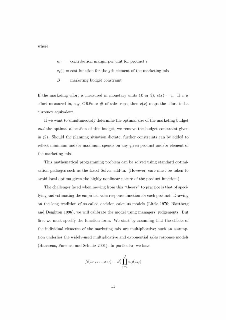
where

mi = contribution margin per unit for product i

cj(·) = cost function for the jth element of the marketing mix

B = marketing budget constraint

If the marketing effort is measured in monetary units (£ or $), c(x) = x. If x is

effort measured in, say, GRPs or # of sales reps, then c(x) maps the effort to its

currency equivalent.

If we want to simultaneously determine the optimal size of the marketing budget

and the optimal allocation of this budget, we remove the budget constraint given

in (2). Should the planning situation dictate, further constraints can be added to

reflect minimum and/or maximum spends on any given product and/or element of

the marketing mix.

This mathematical programming problem can be solved using standard optimi-

sation packages such as the Excel Solver add-in. (However, care must be taken to

avoid local optima given the highly nonlinear nature of the product function.)

The challenges faced when moving from this “theory” to practice is that of speci-

fying and estimating the empirical sales response function for each product. Drawing

on the long tradition of so-called decision calculus models (Little 1970; Blattberg

and Deighton 1996), we will calibrate the model using managers’ judgements. But

first we must specify the function form. We start by assuming that the effects of

the individual elements of the marketing mix are multiplicative; such an assump-

tion underlies the widely-used multiplicative and exponential sales response models

(Hanssens, Parsons, and Schultz 2001). In particular, we have

fi(xi1, . . . , xiJ) = Sbi

J∏j=1

eij(xij)

11

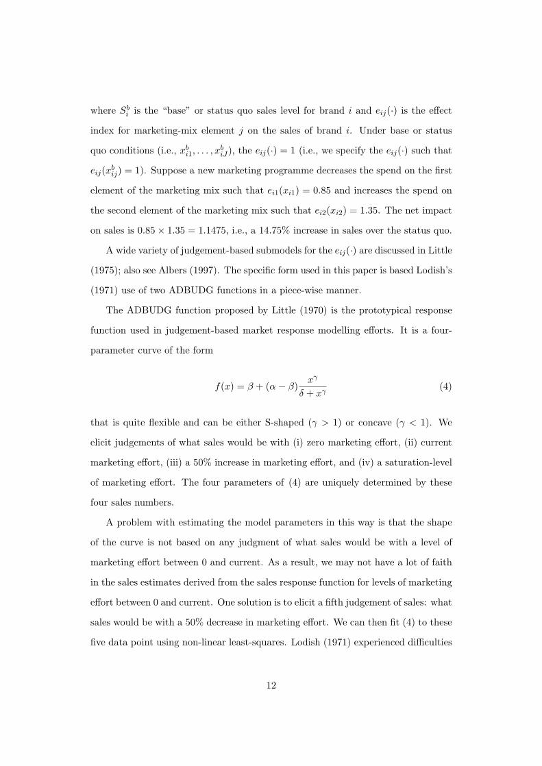
where Sbi is the “base” or status quo sales level for brand i and eij(·) is the effect

index for marketing-mix element j on the sales of brand i. Under base or status

quo conditions (i.e., xbi1, . . . , x

biJ), the eij(·) = 1 (i.e., we specify the eij(·) such that

eij(xbij) = 1). Suppose a new marketing programme decreases the spend on the first

element of the marketing mix such that ei1(xi1) = 0.85 and increases the spend on

the second element of the marketing mix such that ei2(xi2) = 1.35. The net impact

on sales is 0.85 × 1.35 = 1.1475, i.e., a 14.75% increase in sales over the status quo.

A wide variety of judgement-based submodels for the eij(·) are discussed in Little

(1975); also see Albers (1997). The specific form used in this paper is based Lodish’s

(1971) use of two ADBUDG functions in a piece-wise manner.

The ADBUDG function proposed by Little (1970) is the prototypical response

function used in judgement-based market response modelling efforts. It is a four-

parameter curve of the form

f(x) = β + (α − β)xγ

δ + xγ(4)

that is quite flexible and can be either S-shaped (γ > 1) or concave (γ < 1). We

elicit judgements of what sales would be with (i) zero marketing effort, (ii) current

marketing effort, (iii) a 50% increase in marketing effort, and (iv) a saturation-level

of marketing effort. The four parameters of (4) are uniquely determined by these

four sales numbers.

A problem with estimating the model parameters in this way is that the shape

of the curve is not based on any judgment of what sales would be with a level of

marketing effort between 0 and current. As a result, we may not have a lot of faith

in the sales estimates derived from the sales response function for levels of marketing

effort between 0 and current. One solution is to elicit a fifth judgement of sales: what

sales would be with a 50% decrease in marketing effort. We can then fit (4) to these

five data point using non-linear least-squares. Lodish (1971) experienced difficulties

12

with this and therefore used pieces of two ADBUDG functions for different areas

of the response curve. That is, one function is fit through the zero, 50% decrease,

current, and saturation points and is used as the response curve when the marketing

effort is between zero and the current level. Another function is fit through the zero,

current, 50% increase, and saturation points and is used as the response curve when

the marketing effort is above the current level.

Therefore, the functional form we use for the eij(·) is

eij(xij) =

βij + (αij − βij)(xij/xb

ij)γl

ij

δlij + (xij/xb

ij)γl

ij

if xij ≤ xbij

βij + (αij − βij)(xij/xb

ij)γu

ij

δuij + (xij/xb

ij)γu

ijif xij > xb

ij

We estimate the six parameters (αij , βij , γlij , γ

uij , δ

lij , δ

uij) in the following manner.

For each element of the marketing mix for each product, we elicit judgements of

what sales would be with (i) zero marketing effort, (ii) a 50% decrease in marketing

effort, (iii) no change in marketing effort, (iv) a 50% increase in marketing effort,

and (v) a saturation-level of marketing effort. These can be elicited in the following

manner:

Assume that the current sales for product i are indexed at 100. Based

on your knowledge the market, what would have happened to the sales

of this product if it received

• no spend on [element j of the marketing mix]?

• a 50% decrease in effort on [element j of the marketing mix]?

• no change in effort on [element j of the marketing mix]?

• a 50% increase in effort on [element j of the marketing mix]?

• a saturation level of effort on [element j of the marketing mix]?

13

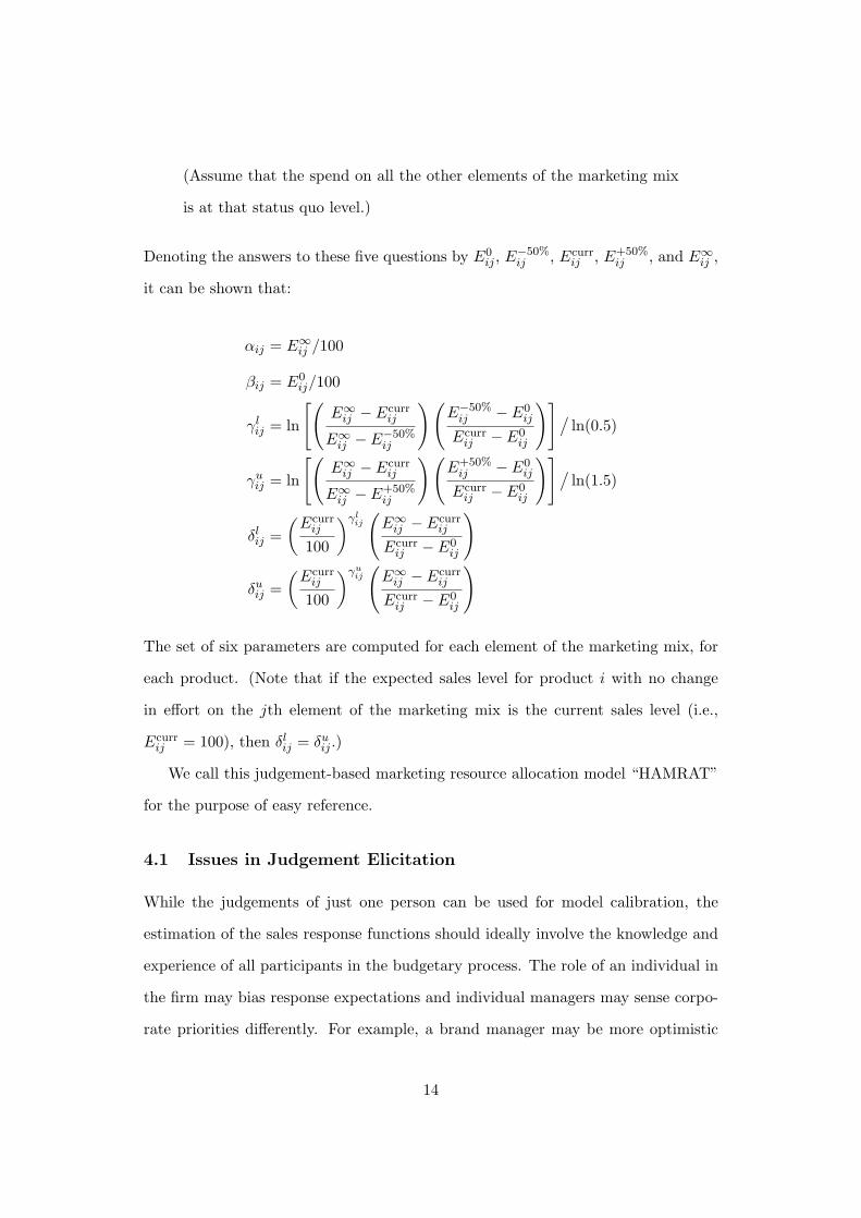
(Assume that the spend on all the other elements of the marketing mix

is at that status quo level.)

Denoting the answers to these five questions by E0ij , E−50%

ij , Ecurrij , E+50%

ij , and E∞ij ,

it can be shown that:

αij = E∞ij /100

βij = E0ij/100

γlij = ln

[(E∞

ij − Ecurrij

E∞ij − E−50%

ij

)(E−50%

ij − E0ij

Ecurrij − E0

ij

)]/ln(0.5)

γuij = ln

[(E∞

ij − Ecurrij

E∞ij − E+50%

ij

)(E+50%

ij − E0ij

Ecurrij − E0

ij

)]/ln(1.5)

δlij =

(Ecurr

ij

100

)γlij

(E∞

ij − Ecurrij

Ecurrij − E0

ij

)

δuij =

(Ecurr

ij

100

)γuij

(E∞

ij − Ecurrij

Ecurrij − E0

ij

)

The set of six parameters are computed for each element of the marketing mix, for

each product. (Note that if the expected sales level for product i with no change

in effort on the jth element of the marketing mix is the current sales level (i.e.,

Ecurrij = 100), then δl

ij = δuij .)

We call this judgement-based marketing resource allocation model “HAMRAT”

for the purpose of easy reference.

4.1 Issues in Judgement Elicitation

While the judgements of just one person can be used for model calibration, the

estimation of the sales response functions should ideally involve the knowledge and

experience of all participants in the budgetary process. The role of an individual in

the firm may bias response expectations and individual managers may sense corpo-

rate priorities differently. For example, a brand manager may be more optimistic

14

about the potential response of his own brand compared to other brands competing

for the same resources.

There are several ways of conducting the estimation procedure:

• Analyst-selected pooling methods:

Several experts provide their estimates. If their opinions are quite similar,

the average of the estimates is used. A substantial similarity of independent

estimates has the effect of heightening the decision-makers’ confidence in the

estimation. On the other hand, should there be substantial divergence in the

estimates of two or more experts, one can either use the estimate of a favoured

expert, or assign some weights for combining the estimates. Winkler (1968)

distinguishes four logical bases for assigning the weights:

1. Equal if the relative expertise of each participant is unknown,

2. Proportional to perceived (by the rest of the team) expertise,

3. Proportional to the experts’ self-ratings of their competence, and

4. Proportional to their past predictive accuracy.

• Group-selected pooling methods:

If the group itself is asked to resolve its differences, there are two common

ways to do this: co-operatively or by the Delphi method.

In a cooperative group, questions or differences are discussed openly, and the

group continues discussion until a single collective answer is reached. Although

very common, this method is viewed with some misgivings because an actual

confrontation of experts is likely to create certain psychological effects that

may spoil the independence of the experts’ estimation processes.

The Delphi estimation procedure (Sackman 1975) has three key features:

1. Anonymous response, in which judgments about sales response of each

brand are obtained formally but anonymously;

15

2. Interaction and controlled feedback, involving open discussions of the

summarised statistical responses of the group

3. Statistical group response, where group opinion is an aggregate of indi-

vidual opinions in the final round.

4. The procedure is repeated several times until group consensus is reached.

If the group reaches a narrow range of inputs indicating similar (credible) max-

ima, then the real world results are unlikely to be sensitive to any solution within

that range.

Quantifying judgements can be a very useful exercise in itself since it ensures

that a problem is given a greater thought, especially if the numbers are a matter of

record. It also pinpoints the extent and importance of differences among executives.

We suggest that the means by which consensus is reached is less important than

the fact that consensus is achieved. Of course, consensus does not imply that the

solution is optimal, only that the group’s intention has been defined. If we find

that the two sets of consensus results emerge, it easy to run the model twice, once

for each set of judgement, to see how sensitive the budgetary allocations are to the

input judgements.

4.2 Extension to the Basic Model

Ambler (2000) recommends that any marketing budgetary process should also report

changes in brand equity. Therefore, in addition to optimising the forecast profit

contribution, HAMRAT estimates the incremental addition to brand equity from the

marketing communications (marcomms) budget. We assume that this is the only

part of the mix to increase brand equity. Should this not be the case, adjustments

would be needed. By “brand equity” we mean “customer-based brand equity” as

defined by Keller (1998).

Of course, if marcomms only affect the plan period, no adjustment for brand

16

equity is needed, otherwise change of brand equity needs to be considered alongside

profit (Ambler 2000). Alternatively, if marcomms are on a maintenance basis, the

brand equity at the end of the plan period will be equal to that at the beginning

and there will be no need to reflect any changes in the brand equity.

While it is possible to do so, we do not combine the profit and brand equity

effects because we believe the short- (plan) and long-term effects, for which the

change in brand equity is a proxy, should be considered separately.

Keller (1998), citing Rubinson (1992), states that brand equity measurement is

essentially multivariate. Whilst we agree with that, our problem was to introduce

some longer term consideration into this type of modelling, perhaps for the first

time. We needed to be economical with the data, not least because users would be

impatient with a large amount of input purely for this secondary effect.

The CEO of Unilever has referred to a brand “as a reservoir, if you like, of future

cash flow” (Fitzgerald 2001, p.22). In other words, the profit that will be earned

as a result of the period’s marcomms, but which was not taken in the period itself,

has topped up the reservoir and can now be used as an estimate of the incremental

brand equity. This is given by the carry-over indicated by the decay estimate. In

other words, if only 70 percent of the budget is burned up, so to speak, in the plan

period, 30 percent of the incremental profits are deemed to fall in the following year.

To the simple estimate of sales, and thus profit, carry-over (Kotler 1997, p. 639),

we additionally factor in the change in share of voice. This second-order effect

reflects the dynamic of the market. It is widely believed (e.g. Kotler 1997, p. 659)

that changing the share of voice will nudge market share in the same direction, other

things being equal.

It follows that the change in brand equity for product i (∆BE i) is calculated as

follows:

∆BE i = Sales i × mi × BEdr i × Forecast SOVi

SOVi

17

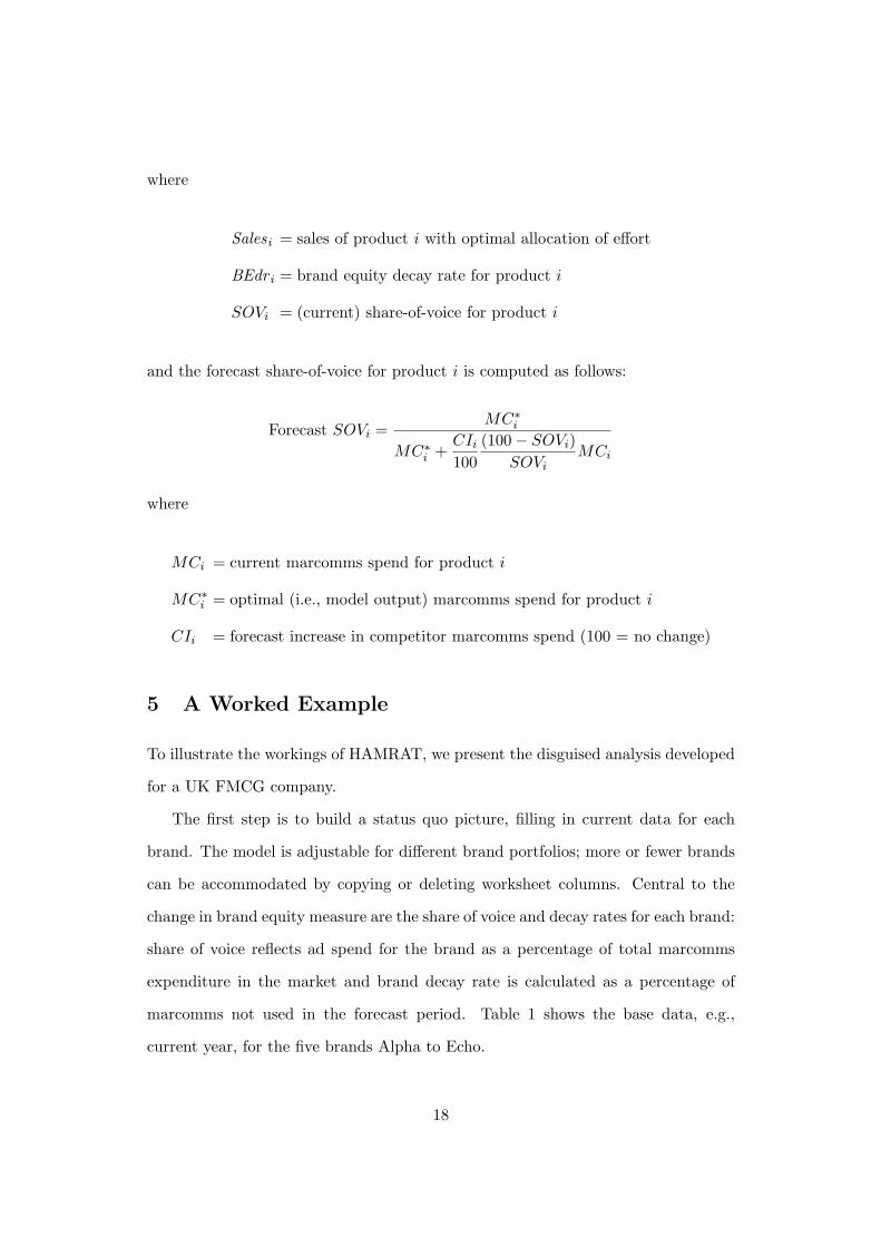
where

Sales i = sales of product i with optimal allocation of effort

BEdr i = brand equity decay rate for product i

SOVi = (current) share-of-voice for product i

and the forecast share-of-voice for product i is computed as follows:

Forecast SOVi =MC∗

i

MC∗i +

CIi

100(100 − SOVi)

SOViMCi

where

MCi = current marcomms spend for product i

MC∗i = optimal (i.e., model output) marcomms spend for product i

CIi = forecast increase in competitor marcomms spend (100 = no change)

5 A Worked Example

To illustrate the workings of HAMRAT, we present the disguised analysis developed

for a UK FMCG company.

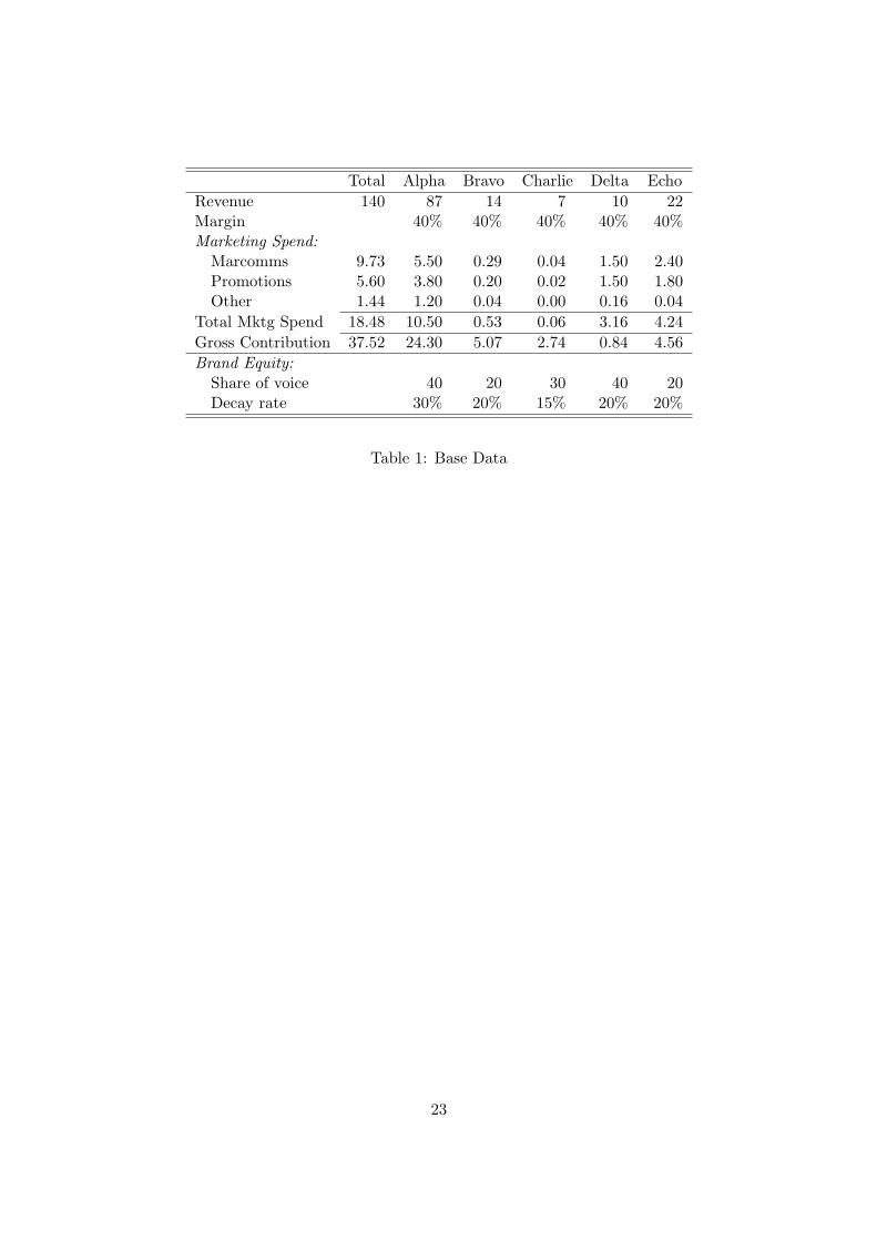
The first step is to build a status quo picture, filling in current data for each

brand. The model is adjustable for different brand portfolios; more or fewer brands

can be accommodated by copying or deleting worksheet columns. Central to the

change in brand equity measure are the share of voice and decay rates for each brand:

share of voice reflects ad spend for the brand as a percentage of total marcomms

expenditure in the market and brand decay rate is calculated as a percentage of

marcomms not used in the forecast period. Table 1 shows the base data, e.g.,

current year, for the five brands Alpha to Echo.

18

——————————————[ Table 1 about here ]

——————————————

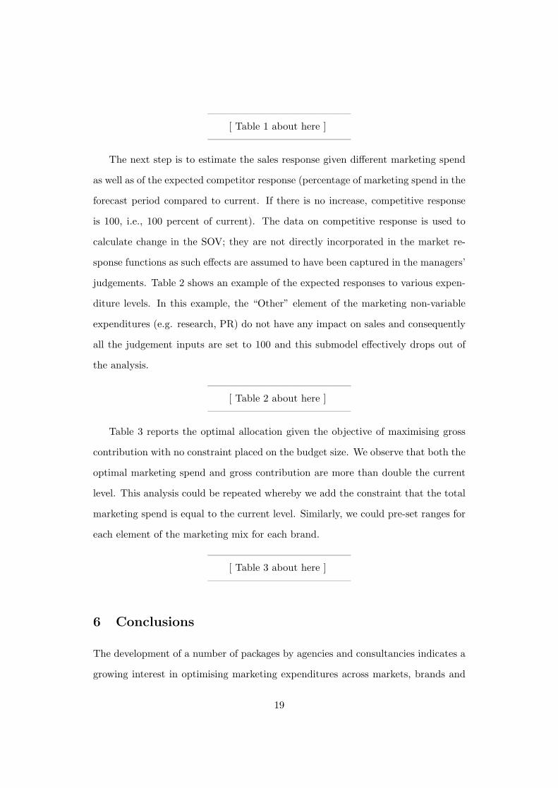
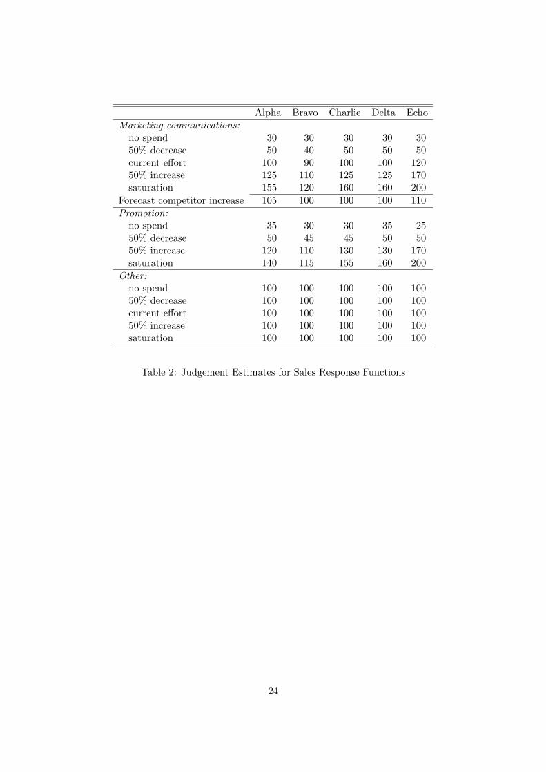
The next step is to estimate the sales response given different marketing spend

as well as of the expected competitor response (percentage of marketing spend in the

forecast period compared to current. If there is no increase, competitive response

is 100, i.e., 100 percent of current). The data on competitive response is used to

calculate change in the SOV; they are not directly incorporated in the market re-

sponse functions as such effects are assumed to have been captured in the managers’

judgements. Table 2 shows an example of the expected responses to various expen-

diture levels. In this example, the “Other” element of the marketing non-variable

expenditures (e.g. research, PR) do not have any impact on sales and consequently

all the judgement inputs are set to 100 and this submodel effectively drops out of

the analysis.

——————————————[ Table 2 about here ]

——————————————

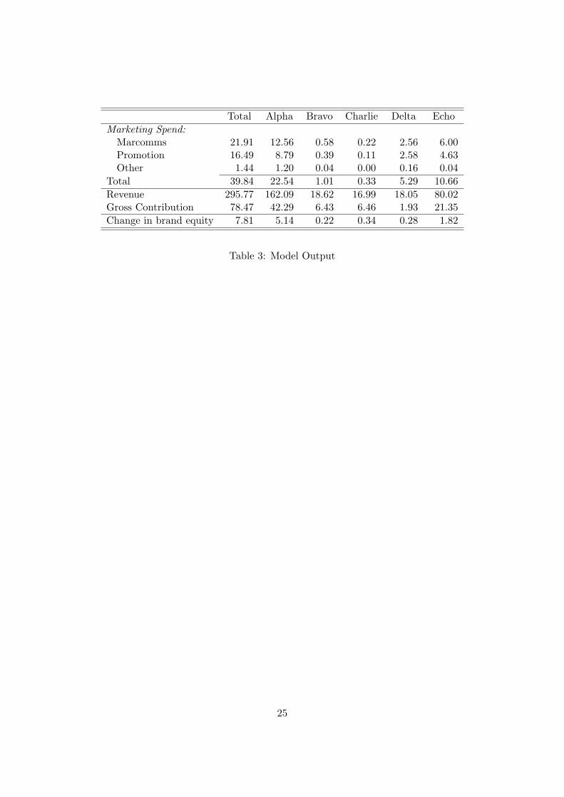
Table 3 reports the optimal allocation given the objective of maximising gross

contribution with no constraint placed on the budget size. We observe that both the

optimal marketing spend and gross contribution are more than double the current

level. This analysis could be repeated whereby we add the constraint that the total

marketing spend is equal to the current level. Similarly, we could pre-set ranges for

each element of the marketing mix for each brand.

——————————————[ Table 3 about here ]

——————————————

6 Conclusions

The development of a number of packages by agencies and consultancies indicates a

growing interest in optimising marketing expenditures across markets, brands and

19

the marketing mix. After briefly reviewing both the theory and practical consid-

erations, we presented HAMRAT as a useful approach to this problem. HAMRAT

is a decision calculus model that can be implemented within an Excel spreadsheet

that combines judgmental estimates of underlying response phenomena in order to

calculate optimal expenditure for each brand and element of the mix. Furthermore,

it reports the changes in brand equity resulting from the optimised allocation of

marketing resources.

Used iteratively it should clarify implicit assumptions about sales response curves

and achieve consensus. Making these assumptions explicit may prove to be the

principle benefit for agency-client relationships. As an open solution, it can be

developed by practitioners for their own purposes or used to benchmark commercial

tools. We share the view that such models should be used interactively by a team of

managers bringing their knowledge and experience to bear on the budgeting process.

The main limitations of this tool include the focus on sales response curves

which do not reflect price variations. Incorporating price as an input would increase

realism but also complexity and demands on the managers providing the required

judgements. Other extensions to this basic model include the explicit integration of

judgemental inputs with historical data to calibrate the market response functions

and an extension from a single period model to a multi-period model that explicitly

incorporates market dynamics.

In practice we expect HAMRAT to develop in the light of usage by practising

managers.

20

References

Albers, Sonke (1997), “CAPPLAN: A Decision-Support System for Planning thePricing and Sales Effort Policy of a Salesforce,” Pricing Strategy & Practice, 5(1), 30–39.

Ambler, Tim (2000), Marketing and the Bottom Line, London: FT Prentice Hall.

Broadbent, Simon (1979), “One way TV advertisements work,” Journal of the Mar-ket Research Society, 21 (3), 139–166.

Broadbent, Simon (1997), Accountable Advertising, Henley on Thames: Admap.

Brody, Ed and Howard Finkelberg (1997), “Allocating Marketing Resources,” inBrand Valuation, (3rd edition, ed. Raymond Perrier), London: Premier Books,149–159.

Davidson, Hugh (1997), Even More Offensive Marketing, London: Penguin.

Day, George S. (1990), Market Driven Strategy, New York: The Free Press.

Deighton, John and Robert C. Blattberg (1996), “Manage Marketing by CustomerEquity Test,” Harvard Business Review, 74 (July–August), 136–144.

Fitzgerald, Niall (2001) “Life and Death in the World of Brands,” Market Leader,14 (Autumn), 17–22.

Gallagher (2001), 26th Gallagher Report Consumer Advertising Survey.

Hanssens, Dominique M., Leonard J. Parsons, and Randall L. Schultz (2001),MarketResponse Models: Econometric and Time Series Analysis, 2nd edition, Boston,MA: Kluwer Academic Publishers.

Hopkins, Claude C (1922), Scientific Advertising, Chicago: NTC Business Books.

Interbrand (2001a), Interbrand’s Most Valuable Brands 2001 Methodology, companyweb-site and discussion with Simon Cole, Director

Interbrand (2001b), “Leveraging Brand Value in a Downturn,” Interbrand Insights,No.2 February.

Kaul, Anil and Dick R. Wittink (1995), “Empirical Generalizations About the Im-pact of Advertising on Price Sensitivity and Price,” Marketing Science, 14 (3),Part 2 of 2, G151–G160.

Keller, Kevin Lane (1998), Strategic Brand Management, Upper Saddle River, NJ:Prentice Hall.

Kotler, Philip (1997), Marketing Management, 9th edition, Upper Saddle River, NJ:Prentice Hall.

Little, John D.C. (1966), “A Model of Adaptive Control of Promotional Spending,”Operations Research, 14 (November), 1075–1097.

21

Little, John D.C. (1970), “Models and managers, the concept of a decision calculus,”Management Science, 16 (April), B466–B485.

Little, John D.C. (1975), “BRANDAID: A Marketing Mix Models. Part 1, Struc-ture, and Part 2, Implementation,” Operations Research, 23 (July–August), 628–673.

Lodish, Leonard M. (1971), “CALLPLAN: An Interactive Salesman’s Call PlanningSystem,” Management Science, 18 (December), P-25–P-40.

Lodish, Leonard M., Ellen Curtis, Michael Ness, and M. Kerry Simpson (1988),“Sales Force Sizing and Deployment Using a Decision Calculus Model at SyntexLaboratories,” Interfaces, 18 (January–February), 5–20.

Lodish, Leonard M., Magid M. Abraham, Jeanne Livelsberger, Beth Lubetkin, BruceRichardson, and Mary Ellen Stevens (1995), “A summary of fifty-five in-marketexperimental estimates of the long-term effects of TV advertising,” MarketingScience, 14 (3), 133–140.

Rao, Vithala R. and Joel H. Steckel (1995), The New Science of Marketing, Chicago,IL: Irwin.

Rohr, J. C., M. Sasserath, and A. Schmidt (1997), “An Integrated Approach to theDevelopment of Leadership Brands: Combining Budget Allocation Issues withthe Management of Brand Values,” ESOMAR Congress.

Rubinson, Joel (1992), “Brand Strength Means More Than Market Share,” ARFFourth Annual Advertising and Promotion Workshop, February 12–13.

Russell, J.Thomas and W. Ronald Lane (2002), Kleppner’s Advertising Procedure,15th edition, Upper Saddle River, NJ: Prentice Hall.

Sackman, Harold. (1975), Delphi Critique, Lexington, MA: Lexington Books.

Urban, Glen L. and Steven H. Star (1991), Advanced Marketing Strategy, EnglewoodCliffs, NJ: Prentice-Hall.

Winkler, R. L. (1968), “The Consensus of Subjective Probability Distributions,”Management Science, 15, B61–B75.

Wisniewski, Kenneth J. and Robert C. Blattberg (1988), “Analysis of ConsumerResponse to Retail Price Dealing Strategies,” Final Report, NSF Grant SES8421165.

22

Total Alpha Bravo Charlie Delta EchoRevenue 140 87 14 7 10 22Margin 40% 40% 40% 40% 40%Marketing Spend:Marcomms 9.73 5.50 0.29 0.04 1.50 2.40Promotions 5.60 3.80 0.20 0.02 1.50 1.80Other 1.44 1.20 0.04 0.00 0.16 0.04

Total Mktg Spend 18.48 10.50 0.53 0.06 3.16 4.24Gross Contribution 37.52 24.30 5.07 2.74 0.84 4.56Brand Equity:Share of voice 40 20 30 40 20Decay rate 30% 20% 15% 20% 20%

Table 1: Base Data

23

Alpha Bravo Charlie Delta EchoMarketing communications:no spend 30 30 30 30 3050% decrease 50 40 50 50 50current effort 100 90 100 100 12050% increase 125 110 125 125 170saturation 155 120 160 160 200

Forecast competitor increase 105 100 100 100 110Promotion:no spend 35 30 30 35 2550% decrease 50 45 45 50 5050% increase 120 110 130 130 170saturation 140 115 155 160 200

Other:no spend 100 100 100 100 10050% decrease 100 100 100 100 100current effort 100 100 100 100 10050% increase 100 100 100 100 100saturation 100 100 100 100 100

Table 2: Judgement Estimates for Sales Response Functions

24

Total Alpha Bravo Charlie Delta EchoMarketing Spend:Marcomms 21.91 12.56 0.58 0.22 2.56 6.00Promotion 16.49 8.79 0.39 0.11 2.58 4.63Other 1.44 1.20 0.04 0.00 0.16 0.04

Total 39.84 22.54 1.01 0.33 5.29 10.66Revenue 295.77 162.09 18.62 16.99 18.05 80.02Gross Contribution 78.47 42.29 6.43 6.46 1.93 21.35Change in brand equity 7.81 5.14 0.22 0.34 0.28 1.82

Table 3: Model Output

25

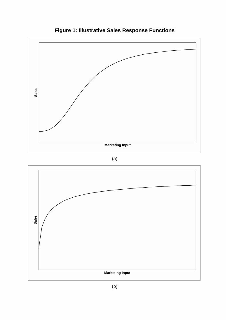
Figure 1: Illustrative Sales Response Functions

(a)

(b)

Marketing Input

Sale

s

Marketing Input

Sale

s