Improving Marine Container Terminal Productivity ... · PDF fileIMPROVING MARINE CONTAINER...
143
The Tioga Group, Inc. 288 Rheem Blvd. Moraga, CA 94556 Phone 925.631.0742 Fax 925.631.7936 IMPROVING MARINE CONTAINER TERMINAL PRODUCTIVITY: DEVELOPMENT OF PRODUCTIVITY MEASURES, PROPOSED SOURCES OF DATA, AND INITIAL COLLECTION OF DATA FROM PROPOSED SOURCES The Tioga Group, Inc. Prepared for: Cargo Handling Cooperative Program July 8, 2010
Transcript of Improving Marine Container Terminal Productivity ... · PDF fileIMPROVING MARINE CONTAINER...
The Tioga Group, Inc.288 Rheem Blvd.Moraga, CA 94556Phone 925.631.0742 Fax 925.631.7936
IMPROVING MARINE CONTAINERTERMINAL PRODUCTIVITY:
DEVELOPMENT OF PRODUCTIVITY MEASURES,PROPOSED SOURCES OF DATA,
AND INITIAL COLLECTION OF DATA FROMPROPOSED SOURCES
The Tioga Group, Inc.
Prepared for:
Cargo Handling Cooperative Program
July 8, 2010
Page iTioga
Contents
I. SUMMARY 1What is the most useful set of productivity metrics? 1Which productivity concepts are used by key stakeholders? 3Recommended Productivity and Utilization Measures 4How can we collect and analyze the required data? 14What is the best approach to benchmarking? 14How can we identify and encourage productivity improvements? 16
II. INTRODUCTION 18Background 18Purpose 19Scope 19Approach 20
III. PORT PRODUCTIVITY CONCEPTS AND DATA SOURCES 21Working Definition of Productivity 21Marine Terminal Capacity and Utilization 22Perspectives on Productivity 24Port Productivity Literature Insights 28Long-term versus Near-term Utilization 31Peak period vs. average productivity 32Customer Survey 33Drayage Survey 35Insights from Rail Intermodal Terminals 36Data Sources 37
IV. PROPOSED PRODUCTIVITY MEASURES 43Approach 43Land Use Measures 43Container Yard Storage Factors 47CY Capacity Measures 55Container Crane Measures 56Vessel Measures 60Berth Measures 66Productivity Implications 71Operating Hours 72Coastal Port Summaries 72Drayage Measures 77Best Drayage Practices 79
V. PROPOSED DATA COLLECTION STRATEGY 84Data Requirements 84Key Barriers to Data Collection 85Data Collection and Publication Options 86Candidate Organizations 86
Page iiTioga
Recommended Strategy 90
APPENDIX A: LITERATURE REVIEW 91Productivity Measurement 91Capacity and Throughput Studies 101Best Practices 105Modeling and Theoretical Approaches 107End Notes 109References 111
APPENDIX B: INSIGHTS FROM RAIL INTERMODAL TERMINALS 115Objective 115Background 115Overview of Rail Terminal Services 116Supplying Rail Terminal Services 117Rail versus Marine Container Moves 118Rail Terminal Productivity Measures 119Rail Intermodal Terminal Development 120Current Development Patterns 123Rail-Marine Comparisons 130Cost Modeling 133Scenarios 134
Page iiiTioga
Exhibits
Exhibit 1: Port and Terminal Data Sources .................................................................................................. 3
Exhibit 2: Results of Customer Survey......................................................................................................... 4
Exhibit 3: Annual TEU per Gross and CY Acre ............................................................................................ 5
Exhibit 4: CY/Gross Acreage Ratio .............................................................................................................. 6
Exhibit 5: TEU Storage Slots ........................................................................................................................ 6
Exhibit 6: TEU Slots per CY Acre (Storage Density).................................................................................... 7
Exhibit 7: Annual TEU per Slot (Turns) ........................................................................................................ 7
Exhibit 8: Annual CY TEU Capacity and 2008 TEU ..................................................................................... 8
Exhibit 9: CY Capacity Utilization ................................................................................................................. 8
Exhibit 10: Annual Vessel Calls per Crane................................................................................................... 9
Exhibit 11: Annual TEU per Crane ............................................................................................................... 9
Exhibit 12: Annual Vessel Calls per Berth .................................................................................................. 10
Exhibit 13: Vessel Size Ratio - - Average versus Maximum TEU .............................................................. 11
Exhibit 14: Vessel Size and Load Ratio...................................................................................................... 11
Exhibit 15: Annual TEU per Berth............................................................................................................... 12
Exhibit 16: Berth Call Utilization ................................................................................................................. 12
Exhibit 17: Berth Utilization - Maximum Vessel Size Basis ........................................................................ 13
Exhibit 18: Five "Dimensions" of Container Terminal Capacity.................................................................. 23
Exhibit 19: Port Utilization Indicators - Canadian Ports.............................................................................. 30
Exhibit 20: Marine Terminal Productivity Concepts.................................................................................... 30
Exhibit 21: LALB Cargo Peaking ................................................................................................................ 32
Exhibit 22: Peaking Impact on Productivity ................................................................................................ 33
Exhibit 23: Customer Survey Respondents................................................................................................ 34
Exhibit 24: Results of Customer Survey..................................................................................................... 34
Exhibit 25: Customer Survey Results–Shifts............................................................................................ 35
Exhibit 26: Port and Terminal Data Sources .............................................................................................. 38
Exhibit 27: Sample Terminal Data .............................................................................................................. 39
Exhibit 28: AAPA TEU Data ....................................................................................................................... 39
Exhibit 29: AAPA Port Data ........................................................................................................................ 40
Exhibit 30: MARAD Vessel Call Data ......................................................................................................... 41
Exhibit 31: Major Ports Analyzed................................................................................................................ 43

Page ivTioga
Exhibit 32: CY/Gross Acreage Ratio .......................................................................................................... 44
Exhibit 33: Seagirt Terminal ...................................................................................................................... 45
Exhibit 34: Hyundai Terminal, Port of Tacoma........................................................................................... 45
Exhibit 35: High Density Outer Harbor Terminal Concept.......................................................................... 46
Exhibit 36: TEU per Gross and CY Acre .................................................................................................... 46
Exhibit 37: Container Yard Handling Equipment Types ............................................................................. 47
Exhibit 38: Progression of Terminal Handling Methods ............................................................................. 48
Exhibit 39: Wheeled Containers on RTG Layout........................................................................................ 49
Exhibit 40: Typical CY Storage Densities ................................................................................................... 51
Exhibit 41: CY Acreage Example: Port of New Orleans............................................................................. 51
Exhibit 42: CY Capacity Example: Port of New Orleans ............................................................................ 52
Exhibit 43: TEU Storage Slots .................................................................................................................... 53
Exhibit 44: TEU Slots per CY Acre (Storage Density)................................................................................ 54
Exhibit 45: Annual TEU per Slot (Turns) .................................................................................................... 55
Exhibit 46: Annual CY TEU Capacity and 2008 TEU................................................................................. 55
Exhibit 47: CY Capacity Utilization ............................................................................................................. 56
Exhibit 48: Typical Two-Berth/Four-Crane Terminal .................................................................................. 58
Exhibit 49: Average Cranes per Berth ........................................................................................................ 58
Exhibit 50: Annual Vessel Calls per Crane................................................................................................. 59
Exhibit 51: Annual TEU per Crane ............................................................................................................. 60
Exhibit 52: DWT vs. Draft ........................................................................................................................... 61
Exhibit 53: USACE Guidance on Cargo Capacity as a Percentage of DWT ............................................. 61
Exhibit 54: Container Vessel DWT vs. TEU Capacity ................................................................................ 62
Exhibit 55: Reported vs. Estimated Container Vessel TEU........................................................................ 63
Exhibit 56: Maximum vs. Average Vessel Capacity - TEU......................................................................... 63
Exhibit 57: Vessel Size Ratio - - Average versus Maximum TEU .............................................................. 64
Exhibit 58: Vessel Size and Load Comparison .......................................................................................... 65
Exhibit 59: Vessel Size and Load Ratio...................................................................................................... 66
Exhibit 60: Berth Capacity - Maximum Vessel Basis Example (Boston).................................................... 68
Exhibit 61: Berth Capacity Estimate- Vessel Call Basis Example.............................................................. 68
Exhibit 62: Annual Vessel Calls per Berth .................................................................................................. 69
Exhibit 63: Annual TEU per Berth............................................................................................................... 69
Page vTioga
Exhibit 64: Berth Call Utilization ................................................................................................................. 70
Exhibit 65: Berth Utilization - Maximum Vessel Size Basis ........................................................................ 71
Exhibit 66: North Atlantic Capacity and Utilization Summary..................................................................... 73
Exhibit 67: South Atlantic Capacity and Utilization Summary .................................................................... 74
Exhibit 68: Gulf Coast Capacity and Utilization Summary.......................................................................... 75
Exhibit 69: West Coast Capacity and Utilization Summary........................................................................ 76
Exhibit 70: Example of Drayage Turn Times.............................................................................................. 77
Exhibit 71: Gate Process Time................................................................................................................... 78
Exhibit 72: Causes of Trouble Tickets ........................................................................................................ 78
Exhibit 73: APM Portsmouth Gate.............................................................................................................. 83
Exhibit 74: Data for Port Metrics................................................................................................................. 84
Exhibit 75: Port Utilization Indicators - Canadian Ports.............................................................................. 91
Exhibit 76: End-loaded Container Terminal Design ................................................................................... 92
Exhibit 77: State of the Art Terminal–CT-A Hamburg .............................................................................. 92
Exhibit 78: Terminal Operating Method Comparison ................................................................................. 93
Exhibit 79: Terminal Capacity versus Container Dwell Time...................................................................... 94
Exhibit 80: Survey of U.S. and Asian Terminals......................................................................................... 94
Exhibit 81: Marine Terminal Productivity Concepts.................................................................................... 95
Exhibit 82: Control Factors in Marine Terminal Productivity....................................................................... 95
Exhibit 83: Port Productivity Comparisons - 2006 ...................................................................................... 96
Exhibit 84: Container Storage Capacity - 2006 .......................................................................................... 96
Exhibit 85: Container Shipping Costs, $/FEU............................................................................................. 97
Exhibit 86: Terminal Productivity Measures ............................................................................................. 101
Exhibit 87: Port of New Orleans Capacity Estimates ............................................................................... 102
Exhibit 88: Container Yard Operating Parameters ................................................................................... 102
Exhibit 89: Assumptions in JWD Long Beach Capacity Study................................................................. 103
Exhibit 90: Port of Long Beach Terminal Capacities ................................................................................ 103
Exhibit 91: San Bernardino, June 1994.................................................................................................... 121
Exhibit 92: San Bernardino, June 2009.................................................................................................... 121
Exhibit 93: Hobart Yard, May 1994........................................................................................................... 122
Exhibit 94: Hobart Yard, July 2007 ........................................................................................................... 122
Exhibit 95 Heartland Corridor ................................................................................................................... 124
Page viTioga
Exhibit 96 Logistics Park Chicago ............................................................................................................ 125
Exhibit 97: Yard Crane and Container Stacking Area at Hobart .............................................................. 126
Exhibit 98: Chassis Stacking .................................................................................................................... 126
Exhibit 99: BNSF SIG, August 2004......................................................................................................... 127
Exhibit 100: BNSF SIG, December 2007 ................................................................................................. 127
Exhibit 101: West End of Croxton Yard .................................................................................................... 128
Exhibit 102: BNSF Hobart and Satellite Yards ......................................................................................... 129
Exhibit 103: Maher Marine Terminal and Remote Lots, Port Elizabeth ................................................... 129
Exhibit 104: On-Site Trackage Changes, Hobart Yard, June 2009.......................................................... 132
Exhibit 105: Tioga Terminal Model Sample Output.................................................................................. 133
Exhibit 106: Cost Comparisons ................................................................................................................ 135
Page 1Tioga
I. Summary
Containerized trade is a vital part of the U.S. and world economies. The efficiency ofcontainerized trade gives U.S. consumers access to imports, and U.S. exporters access to worldmarkets. That efficiency begins at the ports and marine terminals that handle containers,making their productivity a matter of great concern.
This project was undertaken by The Tioga Group, Inc. on behalf of the Cargo HandlingCooperative Program (CHCP), a public-private partnership sponsored by the United StatesMaritime Administration. CHCP’s mission includes increasing cargo handling productivitythrough the implementation of focused research and development.
The growth of container volumes has affected U.S. ports on all coasts, rail terminals on trans-continental routes, and key intermodal connectors. In the decade 1997-2006, aggregate U.S.container volumes at the top 10 ports grew by 186 percent to 35.6 million TEU. The downturnafter 2006 placed participants in the container shipping industry under pressure to define,defend, and improve their productivity. U.S. container terminals and their workforces arefrequently disparaged for being less productive than the leading Asian and European terminals.Given the issues at stake, it is critical for all participants to have a firm understanding of howvarious productivity measures are properly defined and used, what they do (and do not) implyfor terminal operations, and what long-term factors really determine productivity.
The key questions addressed in this study are:
What is the most useful set of productivity metrics?
Which productivity concepts are used by key stakeholders?
How can we collect and analyze the required data?
What is the best approach to benchmarking?
How can we identify and encourage productivity improvements?
Underlying these analytic questions are two more fundamental issues facing port authorities andmarine terminal operators:
Who is my customer and what does he want?
How do I measure what my customer wants?
What is the most useful set of productivity metrics?
Productivity can most usefully be defined as the combined result of resource utilization andoperational efficiency. Resource utilization measures output against capacity, and is usuallyexpressed as a percentage. Productivity of a given asset may be increased either by increasingutilization or by increasing operating efficiency. For example, crane productivity could be
Page 2Tioga
increased by operating cranes more hours each day (utilization) or by achieving more lifts peroperating hour (efficiency).
There are several possible ways to estimate container port capacity, utilization, and productivity.All rely heavily on industry rules of thumb and a variety of assumptions as well as quantifiablerelationships. The general approach used in this study was chosen primarily to suit the readilyavailable port and terminal data elements, with the anticipation of regular data collection,analysis, and publication. More precise estimates are possible, but would require a much greaterinvestment in data collection and analysis, and would change frequently as ports and terminalschange their facilities and operations.
Data to support productivity metrics can be drawn from a number of sources. As Exhibit 1indicates, most of the required data come from the ports or published port directories and fallinto four groups based on relative availability.
Data elements that are almost invariably available from ports, public directories,or government agencies such as the Bureau of Transportation Statistics (BTS).These areshown as “Always” data on Exhibit 1.
Data elements that are often, but not consistently available. These are nottypically confidential and help complete the productivity picture. These dataelements are shown as “Sometimes” dataon Exhibit 1 .
Data that must ordinarily be estimated are also shown on Exhibit 1. These are notroutinely collected or calculated, but are helpful to an understanding ofproductivity. These estimates will have different values depending on theestimation method used.
Cost or labor-related data are usually confidential, as shown on Exhibit 1 andrarely made publicly available. Here too, data values can depend uponmethodology and assumptions that vary from port to port.
Exhibit 1 also illustrates the differences in availability of data on the port as a whole and onindividual terminals. The chief difference is in three data items that are ordinarily available forports but not for terminals:
Annual twenty-foot equivalent units (TEU). The lack of terminal-specific annualTEU eliminates many possible productivity measures for individual terminals(except, of course, for ports such as Savannah, New Orleans, Boston, andPortland that have only one container terminal).
Vessel calls. Vessel call information is collected by estuary or waterway, and isnot always port-specific. The most notable example of this is the Delaware RiverPorts--Philadelphia, Wilmington, and Camden--where data are consolidated byBTS. A similar situation exists for San Francisco Bay.
Vessel deadweight tons (DWT and TEU capacity). Vessel DWT and TEU dataare handled in the same way as vessel calls.

Page 3Tioga
Exhibit 1: Port and Terminal Data Sources
Available Port Data Source Available Terminal Data Source
Berth Depth Port, Directories Berth Depth Port, Directories, TerminalBerth Length Port, Directories Berth Length Port, Directories, TerminalBerths Port, Directories Berths Port, Directories, TerminalChannel Depth Port, Directories Channel Depth Port, Directories, TerminalCranes & Types Port, Directories Cranes & Types Port, Directories, TerminalGross Acres Port, Directories Gross Acres Port, Directories, TerminalPort TEU Port, Directories, AAPAVessel Calls BTS Avg. Crane Moves/hr TerminalVessel DWT BTS CY Acres Port, Terminal
Rail Acres Port, TerminalTEU Slots Port, Terminal
Avg. Crane Moves/hr Port Truck Turn Times TerminalCY Acres Port, Directories Trouble Ticket % TerminalRail Acres Port, DirectoriesTEU Slots Port, Terminals Net BGY Acres Aerial Photos, Terminal Plans
Vessel TEU DWT/TEU RelationshipNet BGY Acres Aerial Photos, Terminal Plans Vessel Length DWT/Length RelationshipVessel TEU DWT/TEU Relationship Avg. Dwell Time Benchmarks, AssumptionsVessel Length DWT/Length Relationship Berth Capacity Benchmarks, AssumptionsAvg. Dwell Time Benchmarks, Assumptions Crane Capacity Benchmarks, AssumptionsBerth Capacity Benchmarks, Assumptions CY Capacity Benchmarks, AssumptionsCrane Capacity Benchmarks, AssumptionsCY Capacity Benchmarks, Assumptions Costs Modeling?
Man-hours Modeling?Costs Modeling? Vessel Turn Time Modeling?Man-hours Modeling? Rates Modeling?Vessel Turn Time Modeling? Working Crane Hours Modeling?Rates Modeling? Terminal TEU Modeling?Working Crane Hours Modeling? Vessel Calls Modeling?
Vessel DWT Modeling?
Confidential
Confidential
Always
Sometimes
Estimated
Always
Sometimes
Estimated
Which productivity concepts are used by key stakeholders?
Discussions of productivity measures in the literature tend to converge on relatively few metrics,listed below.
Annual TEU per acre (or hectare)
Annual TEU per berth (or per foot of berth)
Crane moves (or TEU) per hour (or year)
Vessel turn time (in hours or minutes)
Berth utilization (in percent)
TEU or crane moves per man-hour
Analysis undertaken suggests that some of these concepts are too limited, and that moreinsightful productivity, capacity, and utilization metrics can be developed from readily availabledata.
Customer-focused assessments or competitiveness comparisons, tend to focus on a different, butoverlapping set of measures.
Terminal handling cost (or overall cost)
Cargo velocity, transit time, or dwell time
Vessel turn time
Reliability (e.g. % of moves on schedule)
Page 4Tioga
Crane moves per hour
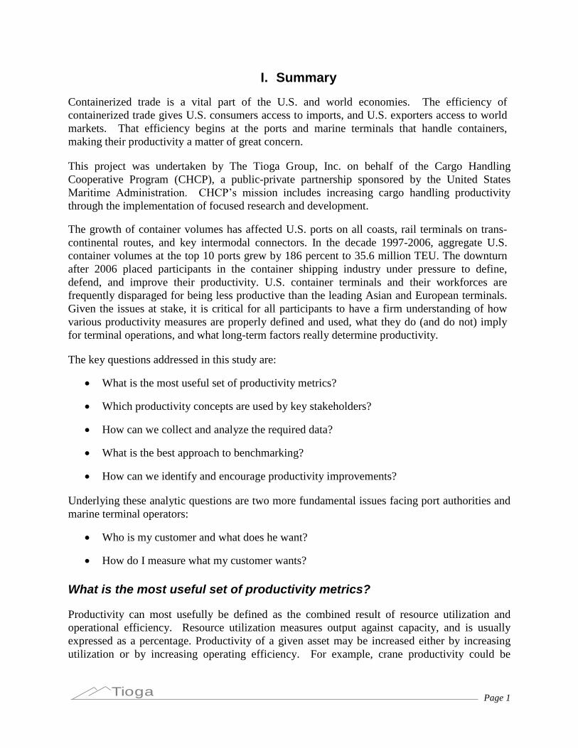
A customer survey taken in this study (Exhibit 2) found much more emphasis on results, such asoverall cost and transit time, than on productivity measures that reflect asset performance. Thissurvey targeted the end customers--importers, exporters, and 3PLs. Those stakeholders do notsee the separate cost of marine terminal operations since it is part of the ocean carrier rate. Theyare likewise insulated from issues such as labor productivity or land use.
Exhibit 2: Results of Customer Survey
As in virtually all industries, cost and labor-related data for marine container terminals areconfidential, and are not accessible for public distribution.
Recommended Productivity and Utilization Measures
The value in the productivity, capacity, and utilization measures recommended below is in theircombined implications for port and terminal performance.
Each terminal is different. Ports, which are collections of terminals, are more different still. Noone measure will suffice, as the differences between ports and the interrelated nature of themetrics create multiple possible interpretations for single data elements. For example, the Port ofHouston’saverage TEU per acre dropped when the new Bayport terminal opened. The overallcapacity and efficiency of the port went up, but, because the new capacity was not immediatelyfilled, a common productivity measure went down. Such instances are common, and dictate theneed for multiple metrics.
The study divided container terminal metrics into groups corresponding to the basic assets beingused:
terminal land and container yard

Page 5Tioga
container cranes
berths and vessels.
Each proposed metric is discussed below, and graphics provide data and comparisons for U.S.mainland container ports. All data are for 2008, as the extreme recession-induced trade declinesin 2009 would drastically skew the metrics.
Land Use and Container Yard (CY) Metrics
Annual TEU per Gross and CY Acre. TEU per acre, meaning gross terminal or port acres, is acommonly used but deceptive metric. Many U.S. container terminals devote substantial portionsof their footprint to rail yards or ancillary facilities that would not be present in Asian orEuropean terminals. Annual TEU per CY acre is a much more revealing metric, as it comparesthroughput (annual TEU) with the inputs directly used (CY acres). Exhibit 3 shows bothmeasures for comparison.
Exhibit 3: Annual TEU per Gross and CY Acre
-
2,000
4,000
6,000
8,000
10,000
12,000
Boston
NYNJ
Delawar
e River
Baltim
oreVPA
APMPorts
mouth
Charles
ton
Savan
nah
Jack
sonvil
le
PortEve
rglad
es
Miami
Mobile
NewOrle
ans
Houston
LALB
Oaklan
d
Portlan
d
Seattl
e
Tacom
a
U.S. M
ainlan
dPorts
Annual TEU/Gross AcreAnnual TEU/CY Acre
The highest figures are associated with the busiest, most intensively used ports, notably LosAngeles-Long Beach (LALB); the Virginia Ports (VPA, including Norfolk, Portsmouth, andHampton Roads); New York-New Jersey (NYNJ); Houston; and Tacoma.
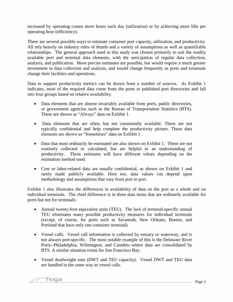
CY/Gross Acreage Ratio. The ratio of CY acres to total (gross) acres helps characterize theport’s land use pattern and sheds light on the interpretation of other metrics. Ports and terminalswith on-dock rail will have lower ratios, as will legacy or combination terminals that includenon-container functions.
Page 6Tioga
Exhibit 4: CY/Gross Acreage Ratio
49%
59%
29%
50%
42%
34%
43% 41%
33%
72%
58%62% 63% 62%
58%
38%
56% 57%52%
50%48% 50%
45%
48%
85%
0%
10%
20%
30%
40%
50%
60%
70%
80%
90%
Boston
NYNJ
Delawar
e River
Baltim
oreVPA
APMPorts
mouth
N. Atla
nticPorts
Charles
ton
Savan
nah
Jack
sonvil
le
PortEve
rglad
es
Miami
S. Atla
nticPorts
Mobile
NewOrle
ans
Houston
GulfPorts
East &
GulfCoas
t PortsLALB
Oaklan
d
Portlan
d
Seattl
e
Tacom
a
Wes
t Coast Ports
U.S. M
ainlan
dPorts
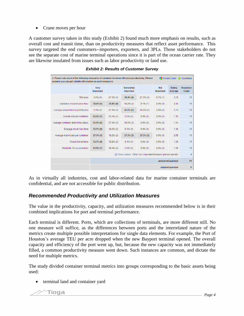
TEU Storage Slots (CY Slot Capacity). The total TEU storage slots in a terminal or portreflects the combination of CY acreage and the CY operating methods in use, and characterizesstatic storage capacity (Exhibit 5). There are two factors at play: CY acreage and stackingdensity. The combination highlights the enormous total capacity at the Ports of Los Angeles andLong Beach. Were Seattle and Tacoma combined in the data, the combination would look muchlarger than the two individual ports.
Exhibit 5: TEU Storage Slots
11,900
125,320
15,000
44,660
23,700
55,180
12,480
243,180
72,980
12,320
40,18041,400
23,080
47,040 42,140
129,260
55,840
16,040
117,960
-
50,000
100,000
150,000
200,000
250,000
Boston
NYNJ
Delawar
e River
Baltim
oreVPA
APMPorts
mouth
Charles
ton
Savan
nah
Jack
sonvil
le
PortEve
rglad
es
Miami
Mobile
NewOrle
ans
Houston
LALB
Oaklan
d
Portlan
d
Seattl
e
Tacom
a
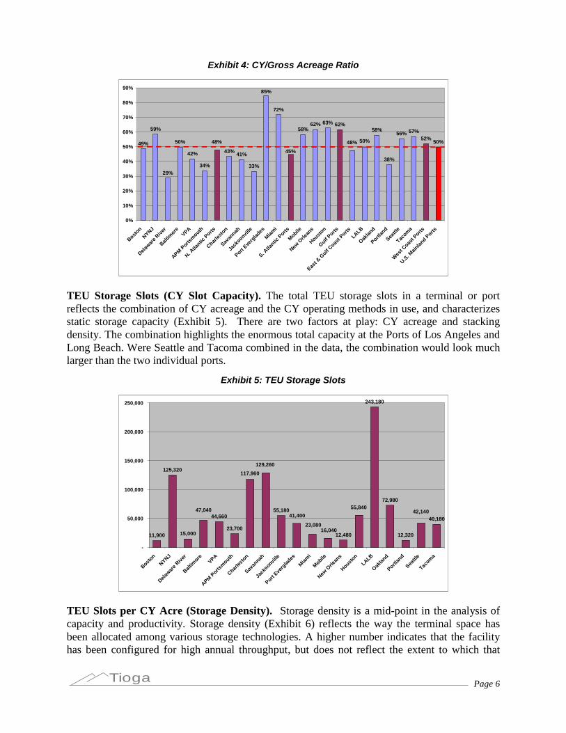
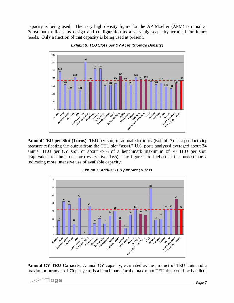
TEU Slots per CY Acre (Storage Density). Storage density is a mid-point in the analysis ofcapacity and productivity. Storage density (Exhibit 6) reflects the way the terminal space hasbeen allocated among various storage technologies. A higher number indicates that the facilityhas been configured for high annual throughput, but does not reflect the extent to which that
Page 7Tioga
capacity is being used. The very high density figure for the AP Moeller (APM) terminal atPortsmouth reflects its design and configuration as a very high-capacity terminal for futureneeds. Only a fraction of that capacity is being used at present.
Exhibit 6: TEU Slots per CY Acre (Storage Density)
243
160
125
206
124
306
260 261
153 155
214
158
205191 194
178160
143134
185169
165176166174
-
50
100
150
200
250
300
350
Boston
NYNJ
Delawar
e River
Baltim
oreVPA
APMPorts
mouth
N. Atla
nticPorts
Charles
ton
Savan
nah
Jack
sonvil
le
PortEve
rglad
es
Miami
S. Atla
nticPorts
Mobile
NewOrle
ans
Houston
GulfPorts
East &
GulfCoas
t PortsLALB
Oaklan
d
Portlan
d
Seattl
e
Tacom
a
Wes
t Coast Ports
U.S. M
ainlan
dPorts
Annual TEU per Slot (Turns). TEU per slot, or annual slot turns (Exhibit 7), is a productivitymeasure reflecting the output from the TEU slot “asset.”U.S. ports analyzed averaged about 34annual TEU per CY slot, or about 49% of a benchmark maximum of 70 TEU per slot.(Equivalent to about one turn every five days). The figures are highest at the busiest ports,indicating more intensive use of available capacity.
Exhibit 7: Annual TEU per Slot (Turns)
18
4238
47
-
2018
25
32
26
59
18
33 34 32
14
24
13
25
14
20
45
8
30
36
-
10
20
30
40
50
60
70
Boston
NYNJ
Delawar
e River
Baltim
oreVPA
APMPorts
mouth
N. Atla
nticPorts
Charles
ton
Savan
nah
Jack
sonvil
le
PortEve
rglad
es
Miami
S. Atla
nticPorts
Mobile
NewOrle
ans
Houston
GulfPorts
East &
GulfCoas
t PortsLALB
Oaklan
d
Portlan
d
Seattl
e
Tacom
a
Wes
t Coast Ports
U.S. M
ainlan
dPorts
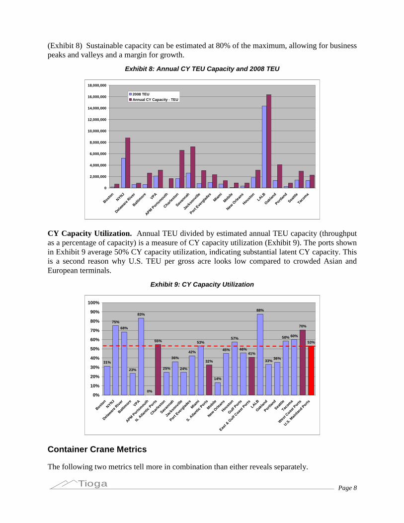
Annual CY TEU Capacity. Annual CY capacity, estimated as the product of TEU slots and amaximum turnover of 70 per year, is a benchmark for the maximum TEU that could be handled.
Page 8Tioga
(Exhibit 8) Sustainable capacity can be estimated at 80% of the maximum, allowing for businesspeaks and valleys and a margin for growth.
Exhibit 8: Annual CY TEU Capacity and 2008 TEU
0
2,000,000
4,000,000
6,000,000
8,000,000
10,000,000
12,000,000
14,000,000
16,000,000
18,000,000
Boston
NYNJ
Delawar
e River
Baltim
oreVPA
APMPorts
mouth
Charles
ton
Savan
nah
Jack
sonvil
le
PortEve
rglad
es
Miami
Mobile
NewOrle
ans
Houston
LALB
Oaklan
d
Portlan
d
Seattl
e
Tacom
a
2008 TEUAnnual CY Capacity - TEU
CY Capacity Utilization. Annual TEU divided by estimated annual TEU capacity (throughputas a percentage of capacity) is a measure of CY capacity utilization (Exhibit 9). The ports shownin Exhibit 9 average 50% CY capacity utilization, indicating substantial latent CY capacity. Thisis a second reason why U.S. TEU per gross acre looks low compared to crowded Asian andEuropean terminals.
Exhibit 9: CY Capacity Utilization
31%
75%
68%
23%
83%
0%
55%
25%
36%
24%
42%
53%
32%
14%
45%
57%
46%41%
88%
33%36%
58% 60%
70%
53%
0%
10%
20%
30%
40%
50%
60%
70%
80%
90%
100%
Boston
NYNJ
Delawar
e River
Baltim
oreVPA
APMPorts
mouth
N. Atla
nticPorts
Charles
ton
Savan
nah
Jack
sonvil
le
PortEve
rglad
es
Miami
S. Atla
nticPorts
Mobile
NewOrle
ans
Houston
GulfPorts
East &
GulfCoas
t PortsLALB
Oaklan
d
Portlan
d
Seattl
e
Tacom
a
Wes
t Coast Ports
U.S. M
ainlan
dPorts
Container Crane Metrics
The following two metrics tell more in combination than either reveals separately.

Page 9Tioga
Annual Vessel Calls per Crane. A marine terminal may use anywhere from one to five cranesto discharge and load a containership. A low number of calls per crane (Exhibit 10) suggests thateither there are relatively few vessel calls or that the average call discharges and loads a largenumber of containers. The low number for LALB is due to the size of the vessels; large vesselsrequire more cranes on each call.
Exhibit 10: Annual Vessel Calls per Crane
3642
62
16
63
-
43
78 79
17
89
6461
14
74
45 4550
21
57
19
27 27 27
37
-
10
20
30
40
50
60
70
80
90
100
Boston
NYNJ
Delawar
e River
Baltim
oreVPA
APMPorts
mouth
N. Atla
nticPorts
Charles
ton
Savan
nah
Jack
sonvil
le
PortEve
rglad
es
Miami
S. Atla
nticPorts
Mobile
NewOrle
ans
Houston
GulfPorts
East &
GulfCoas
t PortsLALB
Oaklan
d
Portlan
d
Seattl
e
Tacom
a
Wes
t Coast Ports
U.S. M
ainlan
dPorts
Annual TEU per Crane. Annual TEU per crane (Exhibit 11) reflects overall port or terminalperformance and balance. A low figure suggests that cranes are being used to handle eitherrelatively few vessels or relatively few TEU from each vessel. The lowest numbers are atBaltimore, Philadelphia, and Portland, which receive relatively few calls. The low figure atOakland reflects excess crane capacity there.
Exhibit 11: Annual TEU per Crane
52,157
90,777
71,860
38,313
74,403
-
86,081
113,745
41,908
123,137
86,704
30,451
94,437
107,803
42,124
30,682
57,354
84,035
76,709 76,12778,441
82,588
53,919
84,54578,799
-
20,000
40,000
60,000
80,000
100,000
120,000
140,000
Boston
NYNJ
Delawar
e River
Baltim
oreVPA
APMPorts
mouth
N. Atla
nticPorts
Charles
ton
Savan
nah
Jack
sonvil
le
PortEve
rglad
es
Miami
S. Atla
nticPorts
Mobile
NewOrle
ans
Houston
GulfPorts
East &
GulfCoas
t PortsLALB
Oaklan
d
Portlan
d
Seattl
e
Tacom
a
Wes
t Coast Ports
U.S. M
ainlan
dPorts

Page 10Tioga
Exhibit 10 and Exhibit 11 together indicate that the ports of Charleston, Savannah, PortEverglades, and New Orleans have very high container-crane productivity. In fact, the situationis more complex, as they combine high crane efficiency (moves per working hour, a metric thatis not consistently available) and a large number of calls by smaller vessels. At Port Everglades,the ratios are artificially increased by inclusion in the data of TEU volumes that are handled bybarge or self-unloading ships without the use of shore-side cranes.
Berth and Vessel Metrics
Annual Vessel Calls per Berth. Exhibit 12 displays annual vessel calls per berth, which is thefirst factor in berth utilization and productivity. There is some ambiguity when terminals have along berth face that can be divided in different ways, as the number of berths can vary from timeto time. These data also show the large number of vessel calls at Charleston, Savannah, and NewOrleans, reflected in the crane productivity metrics.
Exhibit 12: Annual Vessel Calls per Berth
93
62
38
125
-
164
184
28
89
108
149
107
93
105
57
83
59
807573
51 65
19
82
72
-
20
40
60
80
100
120
140
160
180
200
Boston
NYNJ
Delawar
e River
Baltim
oreVPA
APMPorts
mouth
N. Atla
nticPorts
Charles
ton
Savan
nah
Jack
sonvil
le
PortEve
rglad
es
Miami
S. Atla
nticPorts
Mobile
NewOrle
ans
Houston
GulfPorts
East &
GulfCoas
t PortsLALB
Oaklan
d
Portlan
d
Seattl
e
Tacom
a
Wes
t Coast Ports
U.S. M
ainlan
dPorts
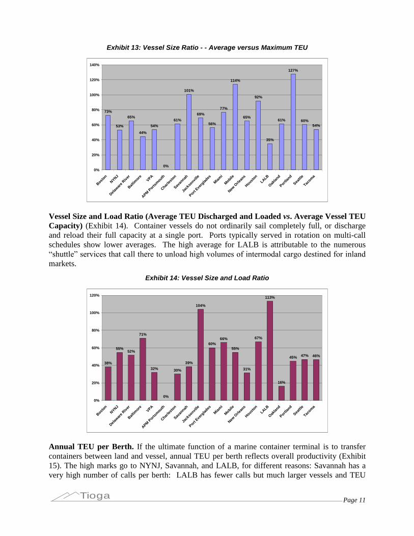
Vessel Size Ratio (Average Vessel TEU Capacity vs. Maximum Vessel TEU Capacity).Comparing the average vessel size being handled to the maximum possible vessel size for theavailable draft (Exhibit 13) indicates how much of the inherent draft and berth length is beingused. This ratio can reach 100% if the port is being served by a fleet of maximum-sized vessels,or if tides or light loading are being used to bring in vessels that would otherwise exceed theavailable draft. Savannah, Mobile, Houston, and Portland show this effect.
Page 11Tioga
Exhibit 13: Vessel Size Ratio - - Average versus Maximum TEU
73%
53%
65%
44%
54%
0%
61%
101%
69%
56%
77%
114%
65%
92%
35%
61%
127%
60%54%
0%
20%
40%
60%
80%
100%
120%
140%
Boston
NYNJ
Delawar
e River
Baltim
oreVPA
APMPorts
mouth
Charles
ton
Savan
nah
Jack
sonvil
le
PortEve
rglad
es
Miami
Mobile
NewOrle
ans
Houston
LALB
Oaklan
d
Portlan
d
Seattl
e
Tacom
a
Vessel Size and Load Ratio (Average TEU Discharged and Loaded vs. Average Vessel TEUCapacity) (Exhibit 14). Container vessels do not ordinarily sail completely full, or dischargeand reload their full capacity at a single port. Ports typically served in rotation on multi-callschedules show lower averages. The high average for LALB is attributable to the numerous“shuttle” services that call there to unload high volumes of intermodal cargo destined for inland markets.
Exhibit 14: Vessel Size and Load Ratio
38%
55%52%
71%
32%
0%
30%
39%
104%
60%66%
55%
31%
67%
113%
16%
45% 47% 46%
0%
20%
40%
60%
80%
100%
120%
Boston
NYNJ
Delawar
e River
Baltim
oreVPA
APMPorts
mouth
Charles
ton
Savan
nah
Jack
sonvil
le
PortEve
rglad
es
Miami
Mobile
NewOrle
ans
Houston
LALB
Oaklan
d
Portlan
d
Seattl
e
Tacom
a
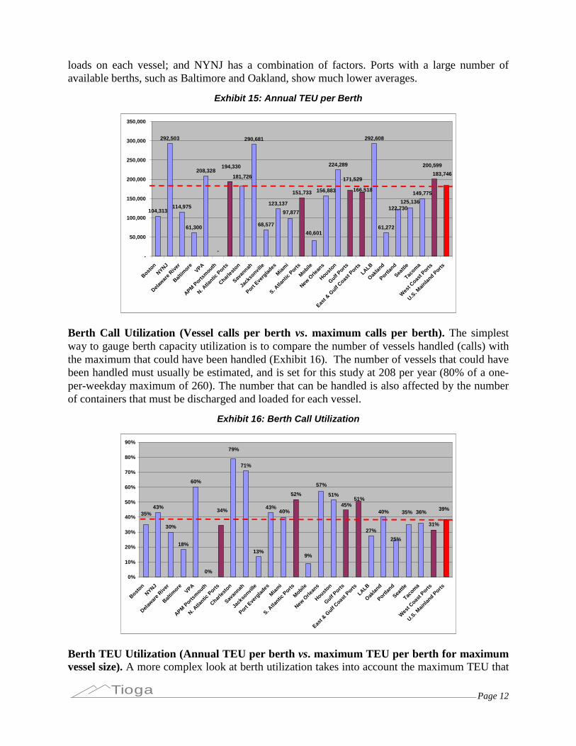
Annual TEU per Berth. If the ultimate function of a marine container terminal is to transfercontainers between land and vessel, annual TEU per berth reflects overall productivity (Exhibit15). The high marks go to NYNJ, Savannah, and LALB, for different reasons: Savannah has avery high number of calls per berth: LALB has fewer calls but much larger vessels and TEU
Page 12Tioga
loads on each vessel; and NYNJ has a combination of factors. Ports with a large number ofavailable berths, such as Baltimore and Oakland, show much lower averages.
Exhibit 15: Annual TEU per Berth
104,313
292,503
114,975
61,300
208,328
-
290,681
68,577
123,137
151,733 156,883
224,289
292,608
61,272
149,775
181,726 171,529
166,518
125,136
183,746
122,730
200,599
40,601
97,877
194,330
-
50,000
100,000
150,000
200,000
250,000
300,000
350,000
Boston
NYNJ
Delawar
e River
Baltim
oreVPA
APMPorts
mouth
N. Atla
nticPorts
Charles
ton
Savan
nah
Jack
sonvil
le
PortEve
rglad
es
Miami
S. Atla
nticPorts
Mobile
NewOrle
ans
Houston
GulfPorts
East &
GulfCoas
t PortsLALB
Oaklan
d
Portlan
d
Seattl
e
Tacom
a
Wes
t Coast Ports
U.S. M
ainlan
dPorts
Berth Call Utilization (Vessel calls per berth vs. maximum calls per berth). The simplestway to gauge berth capacity utilization is to compare the number of vessels handled (calls) withthe maximum that could have been handled (Exhibit 16). The number of vessels that could havebeen handled must usually be estimated, and is set for this study at 208 per year (80% of a one-per-weekday maximum of 260). The number that can be handled is also affected by the numberof containers that must be discharged and loaded for each vessel.
Exhibit 16: Berth Call Utilization
43%
30%
18%
60%
0%
71%
13%
43%
52% 51%
27%
40%35%
57%
36%
79%
45%51%
35%39%
25%
31%
9%
40%34%
0%
10%
20%
30%
40%
50%
60%
70%
80%
90%
Boston
NYNJ
Delawar
e River
Baltim
oreVPA
APMPorts
mouth
N. Atla
nticPorts
Charles
ton
Savan
nah
Jack
sonvil
le
PortEve
rglad
es
Miami
S. Atla
nticPorts
Mobile
NewOrle
ans
Houston
GulfPorts
East &
GulfCoas
t PortsLALB
Oaklan
d
Portlan
d
Seattl
e
Tacom
a
Wes
t Coast Ports
U.S. M
ainlan
dPorts
Berth TEU Utilization (Annual TEU per berth vs. maximum TEU per berth for maximumvessel size). A more complex look at berth utilization takes into account the maximum TEU that
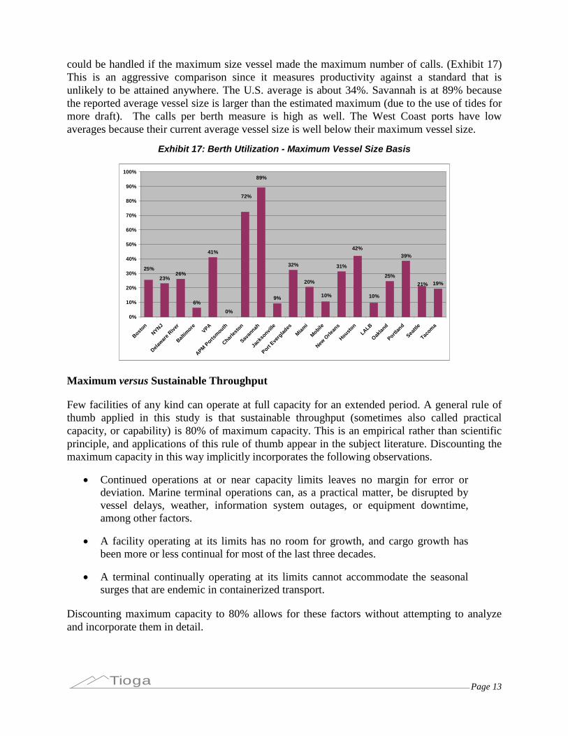
Page 13Tioga
could be handled if the maximum size vessel made the maximum number of calls. (Exhibit 17)This is an aggressive comparison since it measures productivity against a standard that isunlikely to be attained anywhere. The U.S. average is about 34%. Savannah is at 89% becausethe reported average vessel size is larger than the estimated maximum (due to the use of tides formore draft). The calls per berth measure is high as well. The West Coast ports have lowaverages because their current average vessel size is well below their maximum vessel size.
Exhibit 17: Berth Utilization - Maximum Vessel Size Basis
23%26%
6%
41%
0%
9%
32%
20%
31%
25%19%
25%
10%
89%
39%
21%
42%
10%
72%
0%
10%
20%
30%
40%
50%
60%
70%
80%
90%
100%
Boston
NYNJ
Delawar
e River
Baltim
oreVPA
APMPorts
mouth
Charles
ton
Savan
nah
Jack
sonvil
le
PortEve
rglad
es
Miami
Mobile
NewOrle
ans
Houston
LALB
Oaklan
d
Portlan
d
Seattl
e
Tacom
a
Maximum versus Sustainable Throughput
Few facilities of any kind can operate at full capacity for an extended period. A general rule ofthumb applied in this study is that sustainable throughput (sometimes also called practicalcapacity, or capability) is 80% of maximum capacity. This is an empirical rather than scientificprinciple, and applications of this rule of thumb appear in the subject literature. Discounting themaximum capacity in this way implicitly incorporates the following observations.
Continued operations at or near capacity limits leaves no margin for error ordeviation. Marine terminal operations can, as a practical matter, be disrupted byvessel delays, weather, information system outages, or equipment downtime,among other factors.
A facility operating at its limits has no room for growth, and cargo growth hasbeen more or less continual for most of the last three decades.
A terminal continually operating at its limits cannot accommodate the seasonalsurges that are endemic in containerized transport.
Discounting maximum capacity to 80% allows for these factors without attempting to analyzeand incorporate them in detail.
Page 14Tioga
How can we collect and analyze the required data?
The most promising strategy for on-going collection, compilation, and publication of containerport productivity data would involve three organizations.
American Association of Port Authorities (AAPA). The AAPA would collect astandardized set of data elements from its members and publish an annual report.The annual report could be a section of Seaports of the Americas and/or beavailable on-line.
U.S. Maritime Administration (MARAD). MARAD would provide financial orin-kind support and technical assistance, and be the U.S. Department ofTransportation “customer” for whom productivity data would be provided.
The U.S. Army Corps of Engineers Institute for Water Resources/NavigationData Center (USACE IWR/NDC). The U.S. Army Corps of Engineers wouldshare the cost with MARAD and be the federal “customer” for port capacity and infrastructure information supported by the same underlying port data.
This approach would offer the distinct advantage of having the leading industry association andthe two leading federal organizations working from the same data and definitions while sharingthe cost. The resulting data compilations could be made available through AAPA, MARAD,USACE, or the Bureau of Transportation Statistics as required.
Experience in other data collection efforts suggests that an annual update request may be moreeffective than asking for complete data sets every year. In this approach:
AAPA would either collect the initial data or use the data from this study as astarting point.
Each port authority would designate an AAPA contact.
Each year, the AAPA would send each port a form or electronic file showing themost recent data on record and ask the Port Authority for updates and corrections.These data update requests could be combined with existing data submissions ofTEU data to the AAPA.
What is the best approach to benchmarking?
The charts and discussions above, and the more detailed discussions in the body of the report,suggest that great care must be taken in any effort to benchmark productivity, capacity, andutilization of anything so disparate as container ports and terminals. Although each terminal andport uses the same building blocks of land, berths, cranes, etc., they are combined in differentproportions to serve different trades and markets.
Where the nature of the data allow computation of U.S. and regional averages, such figuresprovide at least a starting point for comparisons. U.S. and regional averages are shown in thecharts for the following suggested metrics:
Page 15Tioga
TEU per gross and CY acre (Exhibit 3)
CY/gross acreage ratio (Exhibit 4)
TEU slots per CY acre (storage density) (Exhibit 6)
Annual TEU per slot (turns) (Exhibit 7)
CY capacity utilization (Exhibit 9)
Vessel calls per crane (Exhibit 10)
Annual TEU per crane (Exhibit 11)
Annual vessel calls per berth (Exhibit 12)
Annual TEU per berth (Exhibit 14)
Annual berth call utilization (Exhibit 16)
Estimates of capacity can be made for regions and the U.S. as a whole. These would indicateability to handle future trade rather than relative efficiency, and so are not shown on the charts.Examples include:
TEU storage slots (Exhibit 5)
CY TEU capacity and 2008 TEU (Exhibit 8)
Metrics that relate berth and vessel utilization cannot be reliably defined on a regional basis, inpart because maximum vessel sizes are not meaningful. Some metrics, thus lack useableregional or national averages, including:
Vessel size ratio (average versus maximum TEU) (Exhibit 13)
Vessel size and load ratio (Exhibit 14)
Berth utilization, maximum vessel size basis (Exhibit 17)
As with all benchmarking exercises, comparison between port data and a national average, orbetween two sets of port data, is the beginning point of the analysis, not the end.
Some benchmarks highlight differences in utilization:
CY TEU capacity utilization (Exhibit 9)
Annual TEU per slot (turns) (Exhibit 7)
Annual TEU per crane (Exhibit 11)
Berth call utilization (Exhibit 16)

Page 16Tioga
In these cases low numbers indicate reserve capacity, while high numbers indicate the potentialfor congestion or the need for investment and expansion.
Some benchmarks also highlight characteristics of the trade being handled:
Vessel size ratio (Exhibit 13)
Vessel size and load ratio (Exhibit 14)
These factors are largely external to the ports and terminals, and must be accommodated interminal design and operation.
Still other benchmarks help describe how ports and terminals are configured and used:
CY/Gross acreage ratio (Exhibit 4)
TEU slots per CY acre (storage density) (Exhibit 6)
Vessel calls per crane (Exhibit 10)
These and other benchmarks can be used by port authorities and marine terminal operators tocompare their operations with national averages, and regional competitors to:
Place their operations in context
Highlight key differences
Locate best practices or technologies
Such benchmarks can also be used by regional and national planners and policy makers to:
Assess the ability of ports, coastal systems, and the nation as a whole to handleexpected growth in containerized trade
Locate available short-term capacity for military deployment, export surges,project cargoes, or other specific needs
Assess the adequacy of companion infrastructure in waterways, roads, andrailroads
How can we identify and encourage productivity improvements?
The development and use of port productivity metrics is an essential part of the process ofidentifying and encouraging productivity improvements. That process would include:
Determining what factors of capacity, utilization, and productivity are important
Developing metrics for those factors
Benchmarking to locate high-performing ports
Page 17Tioga
Using multiple metrics to understand variations in performance
Identifying applicable matrices and technologies that make the difference
Productivity metrics will assist ports and public decision makers with much, but not all, of thisprocess. Port specific analysis will still be needed to place individual metrics in context and todetermine why the figures differ.
It is apparent from the productivity metrics and charts presented in this report that “right sizing” is a major factor in high utilization and productivity. Ports, such as LALB and NYNJ, that havebeen hard pressed to expand their terminal areas, exhibit higher densities and utilization. Portsthat have recently added capacity in anticipation of long-term growth, such as Oakland andMobile, show lower short-term utilization and productivity.
Potential high-productivity port examples would include:
LALB, on the basis of TEU per CY acre (Exhibit 3), annual TEU per slot (turns)(Exhibit 7), and vessel size and load ratio (Exhibit 14)
Charleston, on the basis of TEU slots per CY acre (storage density) (Exhibit 6),annual TEU per crane (Exhibit 11), annual vessel calls per berth (Exhibit 12), andberth call utilization (Exhibit 16)
APM Portsmouth, on TEU slots per acre (density) (Exhibit 6)
Specific productivity factors are also cited in the detailed discussions of potential metrics andport data.

Page 18Tioga
II. Introduction
Background
The U.S. economy has been substantially altered by intermodal transportation, which permits theefficient global movement of trade. Economies of scale in vessel, rail, and port operations haveencouraged containerization of a wide variety of import and export commodities. In the decade1997-2006, aggregate U.S. container volumes at the top 10 ports grew by 186 percent to 35.6million TEU.
The capacity and productivity of U.S. container ports is the single most critical factor in thenation’s ability to participate in containerized trade. Beginning in the 1950s and accelerating in the decades that followed, containerization transformed both international merchandise trade andthe ports that serve it. Efficient handling of containerized trade requires far more than justdockside space and labor; it requires sophisticated facilities, equipment, and systems manned bytrained operators. The facilities, equipment, systems, and manpower needed for containerterminals are all costly. There is an inherent tension between having enough capacity for tradepeaks and expected growth, and creating excess capacity that ties up valuable resources.
Participants in the container shipping industry are under pressure to define, defend, and improvetheir productivity. U.S. container terminals and their workforces are frequently disparaged forbeing less productive than the leading Asian and European terminals. Given the issues at stake,it is critical for all participants to have a firm understanding of how various productivitymeasures are properly defined and used, what they do (and do not) imply for terminal operations,and what long-term factors really determine productivity.
There are few, if any, concerns over container port capacity for the immediate future. The globalrecession has drastically eroded containerized trade, with most ports seeing 2009 volumes 10-30percent below the 2006-2007 peaks. Trade began to recover its momentum in early 2010 as thisreport was being prepared, but it will likely take 5-7 years to regain 2006-2007 volumes.
At those 2006-2007 peaks, there were legitimate concerns over the ability of U.S. container portsto accommodate foreseeable long-term growth. The San Pedro Bay ports were severelycongested during the 2004 peak shipping season. Spot capacity shortages have developed fromtime to time at many ports, and have persisted in some cases despite the recession. Given thehigh cost and long lead times required to expand container terminal capacity, it is reasonable toask whether the capacity will be available when it is eventually needed.
The planned opening of the new, higher-capacity Panama Canal locks in 2014 will permitcarriers to deploy larger, more economical vessels in Asia-East Coast and Asia-Gulf services,and challenge the productivity of U.S. ports. The increase in vessel sizes is likely to be gradualas vessel fleets adjust and trade volumes grow. While a gradual increase in the size of trans-Panama container vessels will likely give the U.S. ports time to respond to concomitant capacityneeds, the response will still be necessary.
Page 19Tioga
Purpose
The Cargo Handling Cooperative Program (CHCP) is a public-private partnership sponsored bythe United States Maritime Administration. CHCP’s mission statement includes a general objective to increase the productivity of cargo transportation companies through theimplementation of cargo handling research and development. This project focuses onestablishing an agreed to set of productivity measures for marine terminals. Time-seriescollection of these measures will permit CHCP to benchmark terminal productivity and promotebest practices, allowing CHCP to accomplish its objectives.
The project was completed in two phases. First was the development of the list of measures, andsecond was the collection of the initial set of data.
Scope
There are five basic contexts in which productivity measures are estimated and used.
Port and terminal benchmarking. The primary goal of this project was tofacilitate both cross-section and time-series comparisons. Ports and terminalssometimes conduct their own benchmarking studies or take before-and-aftermeasurements to document the benefits of facility or process improvements.
Cost estimation and planning. From a fiscal standpoint, productivity linksinvestment, operating cost, and revenue. Port and terminal operators useproductivity measures to evaluate and prioritize capital investment projects.
Research and modeling. Private-, academic-, and public-sector researchersexplicitly or implicitly incorporate productivity measures in their analyses andmodels. Examples include the San Francisco Bay Seaport Plan, and models usedto compare terminal configurations and operating practices.
Technology comparisons. Technology firms, equipment vendors, and theirclients all use productivity measures to support decision making.
Port choice and cargo routing. To the extent that carriers and customersconsider port productivity in their choice of import and export ports, productivitymeasures will affect the outcome.
This report does not address the capacity of highways, railroads, and intermodal connectors tomove containers to and from the ports. Trade growth through 2006-2007 was creating concernamong local, regional, and state transportation officials regarding impacts on road and railinfrastructure. The recession has provided a multi-year reprieve, but the issue will eventuallyreturn.
This report likewise does not address the supply of drayage trucks and drivers needed to pick upand deliver more containers. The drayage tractor supply can be increased as required, althoughmeeting stringent emissions requirements will add to the cost. The supply of drivers may bemore problematical. Until the recession, motor carriers nationwide were experiencing a
Page 20Tioga
persistent driver shortage. Some Southern California drayage firms were offering signingbonuses for new drivers. Transportation Worker Identification Credential (TWIC) requirementshave further reduced the pool of drivers eligible for port drayage. As trade recovers, there couldbe a shortage of drayage drivers.
Finally, this report does not address the need for trained personnel to operate expanded terminals.Labor supply cannot be taken for granted. A major contributor to the 2004 peak seasoncongestion in Southern California was a Longshore labor shortage. The pool of Longshore laborhas since expanded, but has shrunk somewhat as Longshoremen idled by the recession havemoved to other jobs.
Approach
The study began by simultaneously reviewing the technical and industry literature to determinehow port productivity could and should be measured, and assembling the available data into a setof marine terminal profiles. These profiles were assembled to serve as the basis for dataanalysis, and are presented as a stand-alone report appendix (Appendix C).
The study team also undertook on-line surveys of major customers (importers, exporters, 3PLs),and drew on surveys of drayage drivers and companies being conducted for other projects. Thestudy team also examined parallel metrics for rail intermodal terminals. Analysis of the datafocused on port productivity, capacity, and utilization metrics that could be developed from datathat were consistently available for major container ports and terminal, or data that is oftenavailable and which could become consistently available. This analysis yielded a set of over 15useable metrics that, together, are far more revealing than global measures, such as TEU pergross acre. These measures can be used to understand the operations of a single port, tounderstand the differences between ports, to benchmark port performance against U.S. averagesor regional revenues, and to locate candidate best practices.

Page 21Tioga
III. Port Productivity Concepts and Data Sources
Working Definition of Productivity
Productivity can most usefully be defined as the combined result of resource utilization andoperational efficiency. Resource utilization measures output against capacity and is usuallyexpressed as a percentage.
For example:
A crane is available 24 hours, and used 8 hours - Utilization = 33%
Operational efficiency measures output per unit input, and is usually expressed as a ratio. Forexample:
A crane averages 24 moves per hour when in use.
Productivity measures output over time. For example:
A crane averages 24 moves/hour, 8 hours/day or–192 moves/day.
Operational efficiency measures output per unit input, and is usually expressed as a ratio. Cranemoves per hour is an efficiency measure, while crane operating hours per day is really autilization measure.
Productivity of a given asset may be increased either by increasing utilization or by increasingoperating efficiency. Using cranes as an example, crane productivity could be increased byoperating cranes more hours per day (utilization) or by achieving more lifts per operating hour(efficiency). This two-part conceptualization of productivity is akin to the DuPont formulationof return on equity (ROE) in corporate finance, where ROE is a function of operating efficiency(profit margin, net profit/sales) and asset efficiency (asset turnover, sales/asset). In both cases,an overall measure is not nearly as useful or revealing as when it is broken into components.
Productivity measures are ordinarily used to compare two methods of obtaining the samethroughput, or the relative throughput of two facilities when both are operating at capacity.Productivity is usually expressed as units of output per unit of input.
TEU per acre/berth/man-hour
Crane moves per hour/day/shift
Moves per gang hour
Cost per TEU/container
Vessels turns per berth
Page 22Tioga
Capacity measures are usually in units of output per time period and should represent themaximum throughput possible unconstrained by demand or other systems.
Maximum TEU per hour/day/year
Maximum crane moves per hour/day
Yard storage TEU/acre
Utilization is usually defined as current throughput divided by throughput capacity, expressed asa percentage.
Berth utilization or occupancy
Crane utilization
Terminal utilization
Throughput is ordinarily expressed in units of output, such as TEU, lifts, or gate transactionsper time period.
Containers per gate hour
Crane moves per hour or day
Vessel turn times
Container dwell time
The distinction is also critical from the perspective of an importer, shipper, or military transportcommand seeking the best way to move cargo. A terminal capable of 10,000 TEU per acre andoperating at 9,000 may be more “productive,”but has less reserve capacity than a terminalcapable of 5,000 TEU per acre but operating at 3,000 TEU.
Marine Terminal Capacity and Utilization
There are several possible ways to estimate container port capacity, utilization, and productivity.All rely heavily on industry rules of thumb and a variety of assumptions as well as quantifiableengineering relationships. The general approach used in this study was primarily chosen to suitthe readily-available port and terminal data elements, with the anticipation of regular datacollection, analysis, and publication. More precise estimates are possible, but would require amuch greater investment in data collection and analysis and would change frequently as portsand terminals change their facilities and operations.
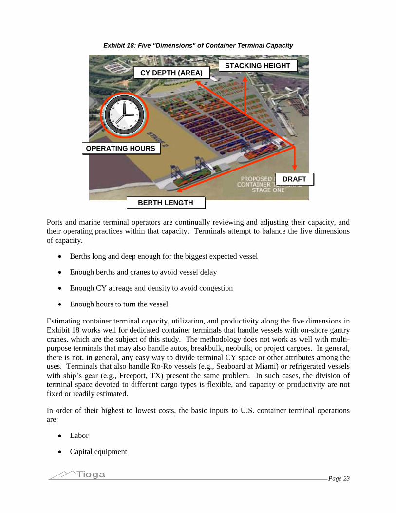
Marine container terminal capacity has five long-term constraints or dimensions, as illustrated inExhibit 18.
Page 23Tioga
Exhibit 18: Five "Dimensions" of Container Terminal Capacity
DRAFTDRAFT
BERTH LENGTHBERTH LENGTH
STACKING HEIGHTSTACKING HEIGHTCY DEPTH (AREA)CY DEPTH (AREA)
OPERATING HOURSOPERATING HOURS
DRAFTDRAFT
BERTH LENGTHBERTH LENGTH
STACKING HEIGHTSTACKING HEIGHTCY DEPTH (AREA)CY DEPTH (AREA)
OPERATING HOURSOPERATING HOURS
Ports and marine terminal operators are continually reviewing and adjusting their capacity, andtheir operating practices within that capacity. Terminals attempt to balance the five dimensionsof capacity.
Berths long and deep enough for the biggest expected vessel
Enough berths and cranes to avoid vessel delay
Enough CY acreage and density to avoid congestion
Enough hours to turn the vessel
Estimating container terminal capacity, utilization, and productivity along the five dimensions inExhibit 18 works well for dedicated container terminals that handle vessels with on-shore gantrycranes, which are the subject of this study. The methodology does not work as well with multi-purpose terminals that may also handle autos, breakbulk, neobulk, or project cargoes. In general,there is not, in general, any easy way to divide terminal CY space or other attributes among theuses. Terminals that also handle Ro-Ro vessels (e.g., Seaboard at Miami) or refrigerated vesselswith ship’s gear (e.g., Freeport, TX) present the same problem. In such cases, the division ofterminal space devoted to different cargo types is flexible, and capacity or productivity are notfixed or readily estimated.
In order of their highest to lowest costs, the basic inputs to U.S. container terminal operationsare:
Labor
Capital equipment
Page 24Tioga
Land
Systems and technology
Accordingly, and rationally, the general container terminal development pattern is as follows.
Terminals start as low-utilization, low-cost operations.
Terminal operators will first seek systems and technology improvements to takemaximum advantage of land, capital equipment, and labor.
As terminal operators reach the limits of existing systems, technology, land, andcapital equipment, they will seek to expand the land available.
When terminal operators have exhausted systems and technology opportunitiesand run out of available land, they will invest in capital equipment to minimizelabor costs.
When terminal operators have exhausted the throughput capabilities of system,technology, land, and capital equipment they will engage more labor.
Within this broad pattern there are detailed variations and exceptions. For example, terminaloperators may find it more efficient on the margin to engage a small amount of additional laborthan to make a large incremental investment in new lift equipment.
Marine container terminals do not ordinarily operate at or near their capacity, nor would we wantthem to do so. A terminal operating at or near its full capacity is highly vulnerable to the leastdisruption and lacks the operating resilience to recover. Moreover, a terminal operating atcapacity has no room for growth, and despite the current downturn in trade, growth will resume.
Perspectives on Productivity
Criteria. Criteria for useful productivity measures might include:
Comparability. The chosen measures should reflect aspects of port and terminalperformance that can reliably be compared across coastal and nationalgeographies.
Accuracy. The measures should be derived through straightforward analysis ofreliable, available data.
Replicability. The effects of year-to-year variations in exogenous factors such asrail industry performance or weather should be noted, and ideally it should bepossible to correct for such variations.
Relevance. The measures should document factors that will enter intooperational choices, capital investments, and cargo routing decisions.
The choice of port productivity metrics should be dictated in large part by their intended use.There are a number of potential users of port performance metrics, including:

Page 25Tioga
terminal operators
labor unions
port authorities
customers (importers, exporters, third parties)
ocean carriers
public agencies
Terminal Operator Perspective. Terminal operators use performance metrics to monitorterminal performance, plan capital expenditures, project revenue, etc. Their primary focus is onthe productivity and efficiency of resources and imports under their control:
labor hours
container cranes
yard equipment
terminal acreage
operating dollars
The highest day-to-day priority of a marine terminal operator is to service the vessel quickly andefficiently. Pertinent productivity measures would include:
crane lifts per hour
crane lifts per man hour
average cost of crane lifts
overall vessel discharge and loading rates
reliability of vessel turn times
High-level measures such as TEU per gross acre are less useful, since they do not translate intomanagement action items. Measures such as container dwell time or storage per acre are moreamenable to management initiative and influence. Measures such as TEU/acre require context: aro-ro terminal operating at 3,000 TEU/acre could be congested while a stacked RTG terminalwould be half empty at the same TEU/acre.
The need for management action or capital investment is most likely to be signaled or triggeredby complaints about growing congestion, escalating unit costs, or lengthening vessel turn timethan by overall throughput or TEU/acre. The most useful metrics would then be those thatenabled management to identify the causes of declining performance and choose among possibleresponses. Rising vessel turn times might be due, for example, to a need for more cranes tohandle larger vessels, inefficient crane operations, or yard delays that waste crane operator time.

Page 26Tioga
Management would need to choose between acquiring more cranes, adding yard equipment, orseeking greater crane operator productivity.
The bottom line for terminal operations is cost. In the short run most terminal assets--land, berthspace, cranes, yard equipment, and systems--are fixed, and longshore labor hours are the keyvariable. Man-hours per lift or an equivalent such as gang-hours per vessel is thus the key near-term operating metric.
This observation highlights a key feature of U.S. container terminals: the high cost of labor andlow cost of land compared to their Asian or European counterparts. It is axiomatic thatcommercial operations will be managed to conserve the scarcest resource, and, in the case ofU.S. container terminals, the scarcest resource is labor.
The 2003 JWD study for the Port of Houston made a crucial observation regarding the reactionof the privately operated APM (Maersk) terminal to growing trade volumes. Once averagethroughput at that terminal reached about 4,000 TEU/acre, the terminal operators aggressivelysought more space. The terminal expanded, keeping TEU/acre at about 4,000, rather thaninvesting in the capital and labor required to increase productivity. Increasing acreage is,ordinarily, a lower cost alternative compared to increasing throughput per acre.
It is reasonable to ask how much terminal operations rely on performance metrics versus theobservations and experience of terminal managers. Does the decision to acquire additional reachstackers depend on a numerical benchmark or on the manager’s conviction that the supply of reach stackers has become a bottleneck? Industry experience suggests that terminal expansion orcapital investment needs are suggested or initiated through management observations, andperhaps vetted or justified by performance metrics.
Carrier Perspective. For marine terminal operators, the primary customers are the oceancarriers. From that perspective:
The highest priority is turning the ship, on time, at lowest cost.
Investment in cranes is sized to vessel size and frequency.
Costs controlled by minimizing labor, particularly second and third shifts.
Flat, wheeled terminals are less expensive to operate.
Vessel conflicts due to high berth utilization are highly undesirable.
Terminal operators are trying to strike a balance between cost and service demands rather thantrying to maximize productivity of any one asset.
Labor Perspective. The increasing sophistication of labor unions and the increased emphasis onthe details of labor union agreements is creating a greater need for labor unions to understandand use productivity measures.
Productivity comparisons between U.S. ports and Canadian, and foreign ports have become partand parcel of longshore contract negotiations. Such comparisons may be used by employer
Page 27Tioga
negotiators to support the need for more flexibility in implementing technologies, or to resistdemands for greater hourly compensation. The upcoming ILA contract negotiations on the EastCoast, for example, have led ILA leadership to investigate industry productivity measures ingreater detail.
The measures of greatest relevance to labor unions are those that express outputs--lifts, annualTEU, gate moves, etc.--as a function of man-hours or labor cost.
In the context of negotiations both sides tend to pick and formulate productivity measures tosupport their position. Comparability and consistency may suffer in the process.
Port Authority Perspective. Port authorities compete for vessel calls and container volume, andproductivity metrics have become factors in that competition. The use of productivity measuresby port authorities will likely vary widely and depend on the context.
Landlord ports, which include most major U.S. container ports, do not participate in terminaloperations management or capital planning for in-terminal equipment. They do, however,negotiate with terminals over lease terms, facility improvements, terminal expansion, and cranes.To the extent that throughput per acre or per crane enters into such negotiations and investmentplans, ports need applicable productivity measures. To the extent that port planning anddevelopment focuses on physical assets, such as land and cranes, the relevant metrics will bethose that express outputs as a function of those inputs. A high level metric such as TEU/acrebecomes relevant when terminal operators are negotiating for more acres.
Where port authorities are also terminal operators, such as at Houston, different performancemetrics will be applied to different decisions. The case of Barbours Cut at the Port of Houston isparticularly notable. As noted earlier, the APM terminal at Houston sought and obtainedadditional terminal acreage to keep density and unit costs under control as container volumesrose. The APM terminal is adjacent to the Barbours Cut terminal, which is operated by the Portof Houston Authority (POHA). As the APM terminal added acreage, Barbours Cut wascorrespondingly constrained. As a result, land utilization at Barbour’s Cut grew while APM’s remained relatively low and constant.
The growing public agency involvement in port planning, access, impacts, and emissions hascreated a need for port authorities to use productivity metrics in external contexts. There isincreasing community concern over port expansion, port truck traffic, port rail traffic, and portemissions. Port productivity has been cited (perhaps unfairly) as an impediment to U.S. exportcompetitiveness. In these circumstances port authorities find themselves compelled to defendtheir use of land (TEU/acre), their cost structure ($/TEU, TEU/man-hour) and their emissions(carbon lbs/TEU, vessel hours in port).
Industry and Shipper Perspective. Based on Tioga’s staffexperience and recent research forCIGMA 20081, ocean carriers and their customers use the following criteria in choosing betweenports and terminals.
1 Containerized Intermodal Goods Movement Assessment, 2008

Page 28Tioga
Capacity–compared to planned shipment volume.
Transit time–compared to supply chain and competitive standards.
Reliability–transit time and cost consistency over time, including peak periods.
Cost–door-to-door cost per unit and in total.
Productivity measures such as lifts per crane hour or TEU/acre are usually relevant to carrier andshipper decisions only to the extent that they affect capacity or cost. A recent OECD report oncontainer port and terminal benchmarking2 lists the factors below as applying to “total port activities.”
Cost–Cost per TEU
Productivity –TEU/hectare of land storage, TEU per berth meter, TEU per unitfor handling equipment
The report states that: “The most useful indicators include the total port cost per TEU and the measures of timeliness.”
The carrier customers (importers and exporters) tend to take for granted those terminalperformance attributes that are commonly available and focus their choice criteria on “scarce attributes.” Until the 2004 peak season congestion in Southern California, adequate terminalcapacity (annual TEU or TEU per acre) was usually assumed, and the physical capability ofterminals to accommodate new cargo was rarely a differentiating factor. Vessel turn timebecame a differentiator with the first of the post-Panamax vessels, which had much largercontainer capacity and a higher daily cost than their predecessors. Rail intermodal capacitybecame an issue after the 1996-98 Union Pacific “meltdown” that slowed Minilandbridge trafficfrom the West Coast. Reliability has become increasingly important as supply chains havetightened and inventory levels have been minimized.
Port Productivity Literature Insights
The literature on container terminal productivity measures is highly varied, comprising tradejournal articles, research reports, academic papers and articles, and conference presentations.There is a parallel and sometimes interwoven literature on the basis of competition between portsand terminals, and on shipper and carrier criteria for choosing ports and terminals. A formalliterature review is presented in Appendix A.
Overall, the available literature provides a strong starting point for CHCP’s inquiry into container port and terminal productivity measurement. There is a strong consensus on thedesirability of measurement, the importance of productivity, and the potential for improvement.There are also cautions expressed regarding comparability, data adequacy, and interpretation.
2http://books.google.com/books?id=87nEhvBZVwcC&pg=PA59&lpg=PA59&dq=terminal+cost+per+TEU&source=bl&ots=oDLbs3zHvv&sig=
Usgq-TqL4l38qlFNku_obPwHa5M&hl=en&ei=32xBSvztF42yswPll7DyCA&sa=X&oi=book_result&ct=result&resnum=9

Page 29Tioga
Technical discussions of productivity measures tend to converge on relatively few metrics,which follow:
Annual TEU per acre (or hectare)
Annual TEU per berth (or per foot of berth)
Crane moves (or TEU) per hour (or year)
Vessel turn time (in hours or minutes)
Berth utilization (in percent)
TEU or crane moves per man-hour
Customer-focused assessments, or competitiveness comparisons, tend to focus on a different, butoverlapping set of measures.
Cargo velocity, transit time, or dwell time
Terminal handling cost (or overall cost)
Vessel turn time
Reliability (e.g. percent of moves on schedule)
Crane moves per hour
Several sources note differences in perspective. There is a noticeable difference in “outside” viewpoints from academia and the public sector, and “inside” viewpoints from industry participants. “Outside” observers tend to focus on overall throughput and productivity measures such as annual TEU, TEU/acre, and TEU/crane. A good example of such discussions is Le-Griffin and Murphy (2007) which uses TEU/foot of berth, TEU/crane, TEU/crane-hour, andTEU/acre.
A 2009 article by Mongelluzzo reporting on the October 7, 2009, Port Productivity Conferencesummarizes presentations and remarks made by multiple speakers. The key points made can besummarized as follows:
Port capacity is currently abundant due to the recession, so the basis ofcompetition will be efficiency rather than capacity.
Productivity will become a challenge for East Coast ports when the third set oflocks allows much larger vessels to transit the Panama Canal starting in 2014.
From the shipping line perspective, the primary productivity concern is lifts perhour, which translates into vessel time in port.
Labor efficiency is a crucial concern because labor costs reportedly account for60-70% of total terminal costs.
Industry participants tend to emphasize either terminal handling costs, vessel turn times, or cranemoves per hour as the basis of competition between ports and terminals. Because terminalhandling charges and port fees are negotiated between ports, terminal operators, and oceancarriers, they are largely confidential. Vessel turn times or crane moves per hour thus become
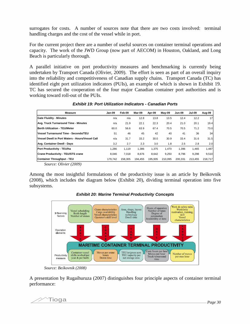
Page 30Tioga
surrogates for costs. A number of sources note that there are two costs involved: terminalhandling charges and the cost of the vessel while in port.
For the current project there are a number of useful sources on container terminal operations andcapacity. The work of the JWD Group (now part of AECOM) in Houston, Oakland, and LongBeach is particularly thorough.
A parallel initiative on port productivity measures and benchmarking is currently beingundertaken by Transport Canada (Olivier, 2009). The effort is seen as part of an overall inquiryinto the reliability and competitiveness of Canadian supply chains. Transport Canada (TC) hasidentified eight port utilization indicators (PUIs), an example of which is shown in Exhibit 19.TC has secured the cooperation of the four major Canadian container port authorities and isworking toward roll-out of the PUIs.
Exhibit 19: Port Utilization Indicators - Canadian Ports
Measure Jan-09 Feb-09 Mar-09 Apr-09 May-09 Jun-09 Jul-09 Aug-09
Gate Fluidity - Minutes n/a n/a 12.8 13.8 13.5 12.4 12.2 17
Avg. Truck Turnaround Time - Minutes n/a 21.9 22.1 22.3 20.4 21.0 20.1 19.4
Berth Utilization - TEU/Meter 60.0 56.6 63.9 67.4 70.5 70.5 71.2 73.0
Vessel Turnaround Time - Seconds/TEU 51 46 45 42 40 41 36 34
Vessel Dwell in Port Waters - Hours/Vessel Call n/a 31.7 33.2 30.0 30.9 33.4 31.6 31.5
Avg. Container Dwell - Days 3.2 2.7 2.3 3.0 1.8 2.5 2.8 2.0
Port Productivity - TEU/ha 1,286 1,119 1,386 1,375 1,470 1,396 1,465 1,487
Crane Productivity - TEU/STS crane 8,046 7,018 8,676 8,642 9,250 8,796 9,298 9,510
Container Throughput - TEU 179,742 158,305 194,455 195,935 210,095 200,331 213,455 218,717
Source: Olivier (2009)
Among the most insightful formulations of the productivity issue is an article by Beŝkovnik(2008), which includes the diagram below (Exhibit 20), dividing terminal operation into fivesubsystems.
Exhibit 20: Marine Terminal Productivity Concepts
Source: Beŝkovnik (2008)
A presentation by Rugaihuruza (2007) distinguishes four principle aspects of container terminalperformance:

Page 31Tioga
Service, where the key factors are vessel turn time and container dwell time
Output, measured by container throughput in TEU
Utilization, including berth occupancy, equipment utilization, and gate utilization
Productivity, in terms of efficiency and cost-effectiveness, measured by (forexample) cost/ton, labor cost/ton, crane moves/hour, containers/man-hour
Both of these sources link specific productivity measures to specific terminal functions andcustomer concerns, thus providing a strong rationale for performance measurement.
The sources examined also provided information on best practices, current or proposed. Some,such as improved management-labor relations, have been issues for decades and are unlikely tobe easily resolved. Others, such as increased use of recent information and location technology,are a logical extension of current initiatives.
Over the last 15 years, there have been numerous efforts in U.S., European, and Asian academiccircles to model container port productivity. The primary technique employed has been DataEnvelope Analysis (also referred to as Data Envelopment Analysis), but other econometrictechniques have been tried as well. While promising and instructive, these efforts have not yetgenerated in results useful to port planners or terminal managers.
Long-term versus Near-term Utilization
In principle, every container yard (CY) acre of every U.S. container terminal could be developedto its maximum long-term capacity. Long-term capacity can be defined as annual TEU storagecapacity using the operating systems with the highest density. At any given point in time, capitalinvestment in terminal equipment and systems to achieve higher densities must be justified bythe expected cargo volumes.
In practice, each terminal is at its own stage of development between the lowest densityoperations (Ro-Ro or wheeled) and the highest density operations (e.g., automated seven-highstacking). Short-term utilization can be defined as current throughput as a percentage of capacityunder the current operating system.
Long-term utilization, in contrast, can be defined as current throughput as a percentage of long-term capacity under the highest density operating system.
With that distinction, container terminals generally fall into three groups.
Low short-term utilization. These terminals have substantial reserve capacitygiven their existing size, operating system, and throughput. Most ro-ro andcombination terminals fall in this category. Such terminals have little or no needto invest in higher productivity systems, although they may risk losing business tocompeting ports with better scale economies and lower unit costs.
Medium short-term utilization. Most dedicated U.S. container terminals fallinto this category, especially given the recession-induced downturn in container
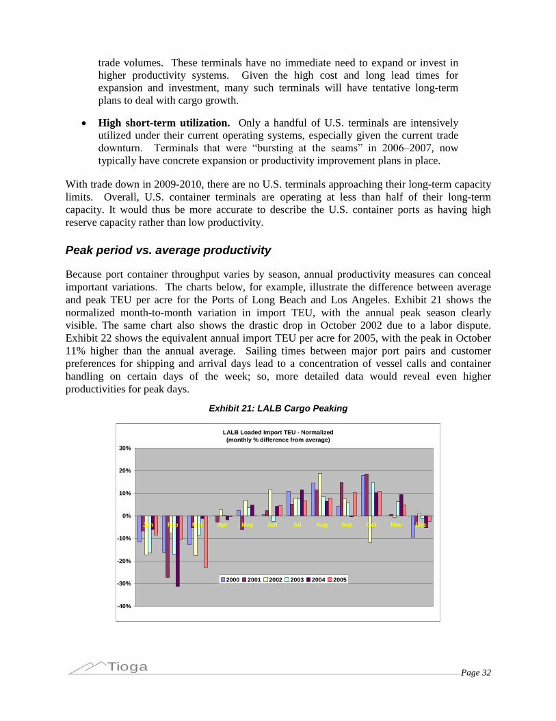
Page 32Tioga
trade volumes. These terminals have no immediate need to expand or invest inhigher productivity systems. Given the high cost and long lead times forexpansion and investment, many such terminals will have tentative long-termplans to deal with cargo growth.
High short-term utilization. Only a handful of U.S. terminals are intensivelyutilized under their current operating systems, especially given the current tradedownturn. Terminals that were “bursting at the seams” in 2006–2007, nowtypically have concrete expansion or productivity improvement plans in place.
With trade down in 2009-2010, there are no U.S. terminals approaching their long-term capacitylimits. Overall, U.S. container terminals are operating at less than half of their long-termcapacity. It would thus be more accurate to describe the U.S. container ports as having highreserve capacity rather than low productivity.
Peak period vs. average productivity
Because port container throughput varies by season, annual productivity measures can concealimportant variations. The charts below, for example, illustrate the difference between averageand peak TEU per acre for the Ports of Long Beach and Los Angeles. Exhibit 21 shows thenormalized month-to-month variation in import TEU, with the annual peak season clearlyvisible. The same chart also shows the drastic drop in October 2002 due to a labor dispute.Exhibit 22 shows the equivalent annual import TEU per acre for 2005, with the peak in October11% higher than the annual average. Sailing times between major port pairs and customerpreferences for shipping and arrival days lead to a concentration of vessel calls and containerhandling on certain days of the week; so, more detailed data would reveal even higherproductivities for peak days.
Exhibit 21: LALB Cargo Peaking
LALB Loaded Import TEU - Normalized(monthly % difference from average)
-40%
-30%
-20%
-10%
0%
10%
20%
30%
Jan Feb Mar Apr May Jun Jul Aug Sep Oct Nov Dec
2000 2001 2002 2003 2004 2005
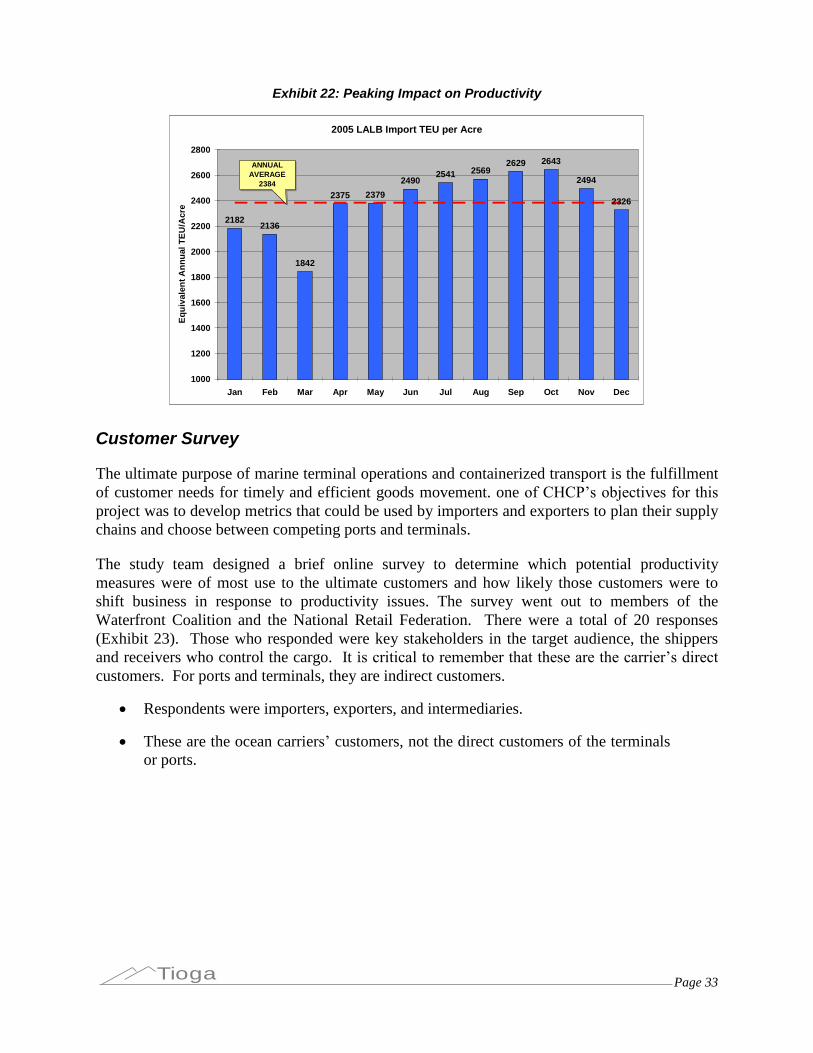
Page 33Tioga
Exhibit 22: Peaking Impact on Productivity
2005 LALB Import TEU per Acre
21822136
1842
2375 2379
24902541 2569
2629 2643
2494
2326
1000
1200
1400
1600
1800
2000
2200
2400
2600
2800
Jan Feb Mar Apr May Jun Jul Aug Sep Oct Nov Dec
Eq
uiv
alen
tA
nn
ual
TE
U/A
cre
ANNUALAVERAGE
2384
Customer Survey
The ultimate purpose of marine terminal operations and containerized transport is the fulfillmentof customer needs for timely and efficient goods movement. one of CHCP’s objectives for this project was to develop metrics that could be used by importers and exporters to plan their supplychains and choose between competing ports and terminals.
The study team designed a brief online survey to determine which potential productivitymeasures were of most use to the ultimate customers and how likely those customers were toshift business in response to productivity issues. The survey went out to members of theWaterfront Coalition and the National Retail Federation. There were a total of 20 responses(Exhibit 23). Those who responded were key stakeholders in the target audience, the shippersand receivers who control the cargo. It is critical to remember that these are the carrier’s direct customers. For ports and terminals, they are indirect customers.
Respondents were importers, exporters, and intermediaries.
These are the ocean carriers’customers, not the direct customers of the terminalsor ports.
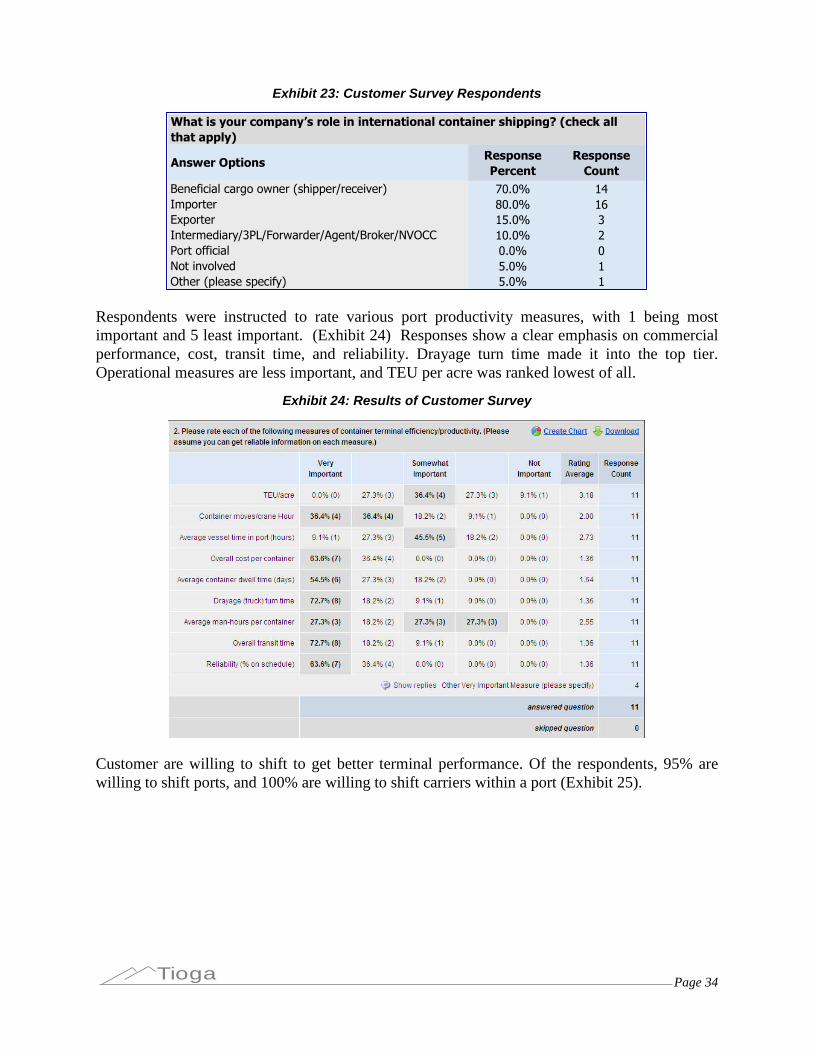
Page 34Tioga
Exhibit 23: Customer Survey Respondents
ResponsePercent
ResponseCount
70.0% 1480.0% 1615.0% 310.0% 20.0% 05.0% 15.0% 1
Exporter
Answer Options
Port official
Importer
Other (please specify)
What is your company’s role in international container shipping? (check all that apply)
Intermediary/3PL/Forwarder/Agent/Broker/NVOCC
Beneficial cargo owner (shipper/receiver)
Not involved
Respondents were instructed to rate various port productivity measures, with 1 being mostimportant and 5 least important. (Exhibit 24) Responses show a clear emphasis on commercialperformance, cost, transit time, and reliability. Drayage turn time made it into the top tier.Operational measures are less important, and TEU per acre was ranked lowest of all.
Exhibit 24: Results of Customer Survey
Customer are willing to shift to get better terminal performance. Of the respondents, 95% arewilling to shift ports, and 100% are willing to shift carriers within a port (Exhibit 25).

Page 35Tioga
Exhibit 25: Customer Survey Results –Shifts
60.0%35.0%5.0%
It depends on...
Would you consider shifting volume between ports basedon container terminal efficiency/productivity?
No
Yes
65.0%35.0%0.0%
It depends on...
Would you consider shifting import or export volumebetween ocean carriers at the same port based on
container terminal efficiency/productivity?
No
Yes
Most of the “It depends on…” answerscentered on cost. If the costs to the customer are equal,customers are willing to shift to get better terminal and drayage performance.
Drayage Survey
Driver surveys were taken at Houston and LALB under parallel project NCFRP-14. There was agood deal of variation on the numbers attributed to the sources of delay. Overall, marineterminals and container depots, including empty yards, were cited as having the most significantsources of delay.
The two most frequently cited issues by drivers are the availability and quality ofchassis, and the tendency for crane and port personnel to divert attention awayfrom truck operations to ship operations when ships are in port.
Other frequently listed complaints regarded the number and availability of liftmachines to service the trucks, being sent to a lane to pick up a container whereno lift machine was available, or several trucks waiting at once for lift machineservice.
Moderate complaints were made about the labor at the ports, especially at LALB.Some drivers pointed to specific issues with port workers on cell phones or whowere otherwise distracted, or shutting down for extended breaks. Others made lessconstructive observations about the port employees being lazy or not sufficientlyskilled to do their jobs.
Wrong information, chassis problems, and empty container problems were citedas the causes of non-revenue trips.
For trouble tickets, equipment problems and information errors were cited as themajor causes.
The primary thing that draymen have learned from their peers is to be sure that allis in readiness before dispatching a driver to a marine terminal
The dominant suggestion as to what marine terminals can do differently is toprovide more workers and to cover breaks rather than to stop work.
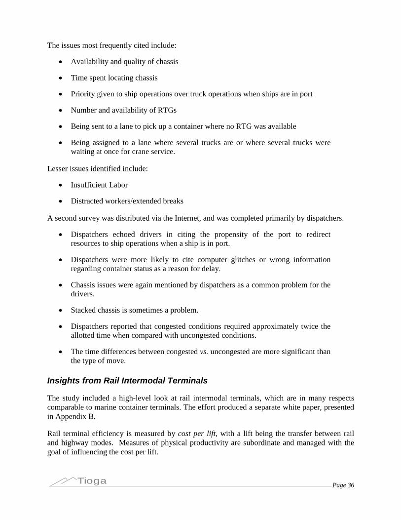
Page 36Tioga
The issues most frequently cited include:
Availability and quality of chassis
Time spent locating chassis
Priority given to ship operations over truck operations when ships are in port
Number and availability of RTGs
Being sent to a lane to pick up a container where no RTG was available
Being assigned to a lane where several trucks are or where several trucks werewaiting at once for crane service.
Lesser issues identified include:
Insufficient Labor
Distracted workers/extended breaks
A second survey was distributed via the Internet, and was completed primarily by dispatchers.
Dispatchers echoed drivers in citing the propensity of the port to redirectresources to ship operations when a ship is in port.
Dispatchers were more likely to cite computer glitches or wrong informationregarding container status as a reason for delay.
Chassis issues were again mentioned by dispatchers as a common problem for thedrivers.
Stacked chassis is sometimes a problem.
Dispatchers reported that congested conditions required approximately twice theallotted time when compared with uncongested conditions.
The time differences between congested vs. uncongested are more significant thanthe type of move.
Insights from Rail Intermodal Terminals
The study included a high-level look at rail intermodal terminals, which are in many respectscomparable to marine container terminals. The effort produced a separate white paper, presentedin Appendix B.
Rail terminal efficiency is measured by cost per lift, with a lift being the transfer between railand highway modes. Measures of physical productivity are subordinate and managed with thegoal of influencing the cost per lift.
Page 37Tioga
Lifts. Activity at intermodal terminals is most commonly measured in lifts. A lift is the transferof a trailer or container from a rail car to the ground/chassis, or from the ground/chassis to railcar. Contract terminal operators are typically paid based on the number of primary lifts theyperform.
Gate transactions. While lifts is the measure of activity for the rail side of the intermodalterminal, gate transactions is the measure of activity for the highway mode. Trucks enter andleave the terminal to deliver and pick up loaded and empty trailers and containers. The truckflow through the terminal can be used as a demand/work measure for gate and clerical personnel.
Railroad terminal operators tend to look and measure terminal productivity in a number ofdifferent ways based on the time horizon in question. The daily issue at an intermodal terminalis how many people and machines are needed for the next shift. The question is answered basedon an estimate of workload for the shift, coupled with knowledge of the equipment and the skilllevel of individual workers. At this level, productivity measures, such as lifts per man hour andproductivity rates for individual operators, are used to size the crews.
Planners with a longer time horizon are typically more interested in longer-term productivityissues involving investments in land, equipment, and facilities. Often these individuals areinvolved in capital investment decisions.
Data Sources
Data to support productivity metrics can be drawn from a number of sources. As Exhibit 26indicates, most of the required data come from the ports or from published port directories. Theexhibit indicates that the source data fall into four groups based on relative availability.
“Always” data. Data elements that are almost invariably available from ports,public directories, or government agencies such as the Bureau of TransportationStatistics (BTS).
“Sometimes” data. Data elements that are often, but not consistently available.These are not typically confidential and help complete the productivity picture.
Estimated data. Data that must ordinarily be estimated, but are helpful to anunderstanding of productivity. These estimates are not routinely collected orcalculated and will have different values depending on the estimation methodused. These estimates often depend heavily on assumptions and industry rules ofthumb.
Confidential data. Cost or labor-related data are usually confidential and rarelymade available outside an organization. Here too, data values can depend uponmethodology and assumptions that vary from port to port.
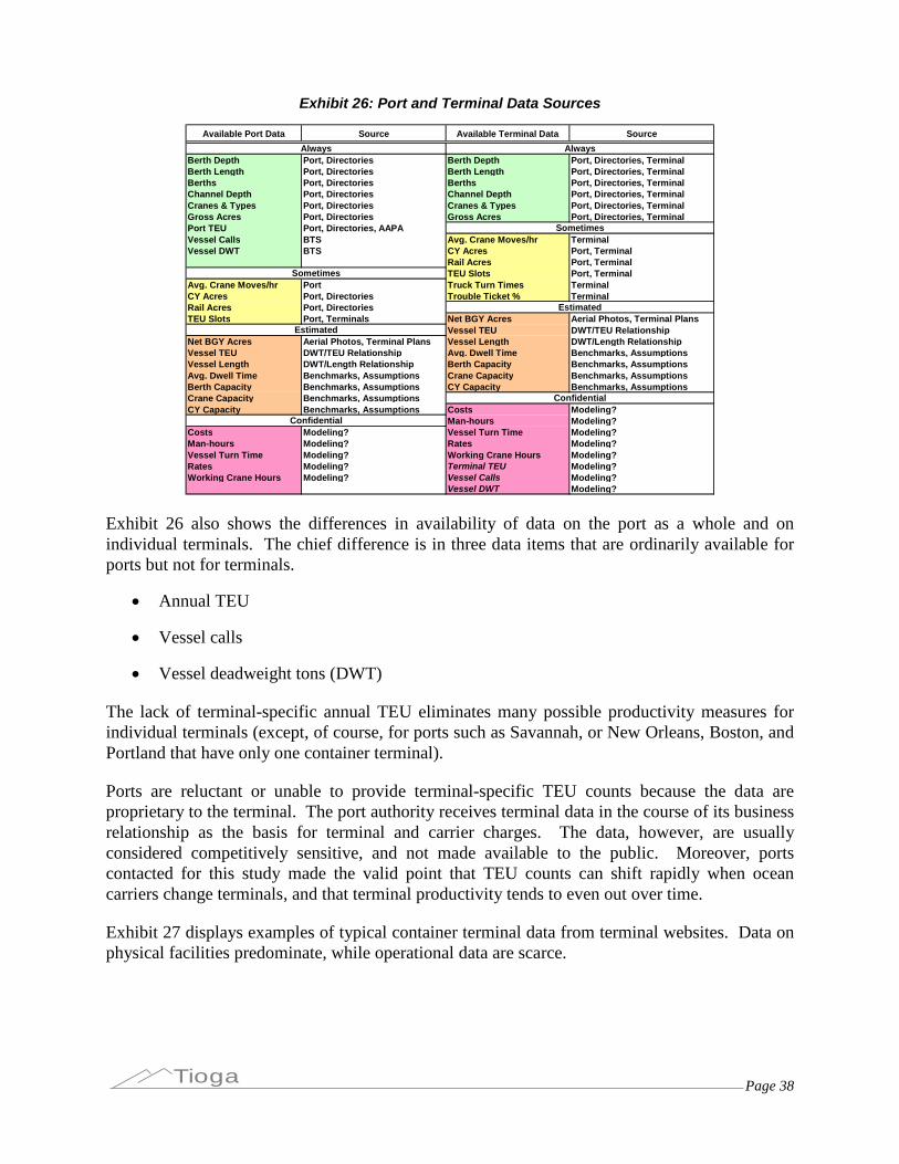
Page 38Tioga
Exhibit 26: Port and Terminal Data Sources
Available Port Data Source Available Terminal Data Source
Berth Depth Port, Directories Berth Depth Port, Directories, TerminalBerth Length Port, Directories Berth Length Port, Directories, TerminalBerths Port, Directories Berths Port, Directories, TerminalChannel Depth Port, Directories Channel Depth Port, Directories, TerminalCranes & Types Port, Directories Cranes & Types Port, Directories, TerminalGross Acres Port, Directories Gross Acres Port, Directories, TerminalPort TEU Port, Directories, AAPAVessel Calls BTS Avg. Crane Moves/hr TerminalVessel DWT BTS CY Acres Port, Terminal
Rail Acres Port, TerminalTEU Slots Port, Terminal
Avg. Crane Moves/hr Port Truck Turn Times TerminalCY Acres Port, Directories Trouble Ticket % TerminalRail Acres Port, DirectoriesTEU Slots Port, Terminals Net BGY Acres Aerial Photos, Terminal Plans
Vessel TEU DWT/TEU RelationshipNet BGY Acres Aerial Photos, Terminal Plans Vessel Length DWT/Length RelationshipVessel TEU DWT/TEU Relationship Avg. Dwell Time Benchmarks, AssumptionsVessel Length DWT/Length Relationship Berth Capacity Benchmarks, AssumptionsAvg. Dwell Time Benchmarks, Assumptions Crane Capacity Benchmarks, AssumptionsBerth Capacity Benchmarks, Assumptions CY Capacity Benchmarks, AssumptionsCrane Capacity Benchmarks, AssumptionsCY Capacity Benchmarks, Assumptions Costs Modeling?
Man-hours Modeling?Costs Modeling? Vessel Turn Time Modeling?Man-hours Modeling? Rates Modeling?Vessel Turn Time Modeling? Working Crane Hours Modeling?Rates Modeling? Terminal TEU Modeling?Working Crane Hours Modeling? Vessel Calls Modeling?
Vessel DWT Modeling?
Confidential
Confidential
Always
Sometimes
Estimated
Always
Sometimes
Estimated
Exhibit 26 also shows the differences in availability of data on the port as a whole and onindividual terminals. The chief difference is in three data items that are ordinarily available forports but not for terminals.
Annual TEU
Vessel calls
Vessel deadweight tons (DWT)
The lack of terminal-specific annual TEU eliminates many possible productivity measures forindividual terminals (except, of course, for ports such as Savannah, or New Orleans, Boston, andPortland that have only one container terminal).
Ports are reluctant or unable to provide terminal-specific TEU counts because the data areproprietary to the terminal. The port authority receives terminal data in the course of its businessrelationship as the basis for terminal and carrier charges. The data, however, are usuallyconsidered competitively sensitive, and not made available to the public. Moreover, portscontacted for this study made the valid point that TEU counts can shift rapidly when oceancarriers change terminals, and that terminal productivity tends to even out over time.
Exhibit 27 displays examples of typical container terminal data from terminal websites. Data onphysical facilities predominate, while operational data are scarce.
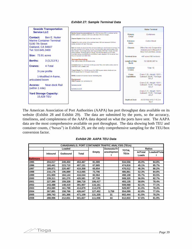
Page 39Tioga
Exhibit 27: Sample Terminal Data
Seaside TransportationService LLC
Contact: Ben E. NutterMarine Container Terminal5190 7th StreetOakland, CA 94607Tel: 510.645.2400
Size: 73.91 acres
Berths: 3 (3,213 ft.)
Cranes: 4-Total
3-Low profile
1-Modified A-frame,articulated boom
Access: Near-dock Rail(within 1 mile)
Yard Storage Capacity:15,628 TEU
The American Association of Port Authorities (AAPA) has port throughput data available on itswebsite (Exhibit 28 and Exhibit 29). The data are submitted by the ports, so the accuracy,timeliness, and completeness of the AAPA data depend on what the ports have sent. The AAPAdata are the most comprehensive available on port throughput. The data showing both TEU andcontainer counts, (“boxes”) in Exhibit 29, are the only comprehensive sampling for the TEU/boxconversion factor.
Exhibit 28: AAPA TEU Data
Inbound Outbound TotalIn/TotalLoads
Loaded/Total
Baltimore1995 204,017 249,450 453,467 81,089 534,556 45.0% 84.8%1996 183,441 223,710 407,151 67,665 474,816 45.1% 85.7%1997 189,871 220,487 410,358 65,654 476,012 46.3% 86.2%1998 216,176 196,889 413,065 73,796 486,861 52.3% 84.8%1999 231,900 184,144 416,044 82,064 498,108 55.7% 83.5%2000 239,311 181,270 420,581 87,739 508,320 56.9% 82.7%2001 227,390 159,328 386,718 106,417 493,135 58.8% 78.4%2002 243,488 148,419 391,907 116,161 508,068 62.1% 77.1%2003 253,080 161,799 414,879 114,078 528,957 61.0% 78.4%2004 267,881 158,766 426,647 127,452 3,759 554,099 62.8% 77.0%2005 289,743 181,366 471,109 131,335 31 602,444 61.5% 78.2%2008 288,996 212,831 501,827 111,006 44 612,833 57.6% 81.9%
CANADIAN/U.S. PORT CONTAINER TRAFFIC ANALYSIS (TEUs)Loaded
EmptyDomestic/Transshipmen
t
TOTALTEUs
Ratios
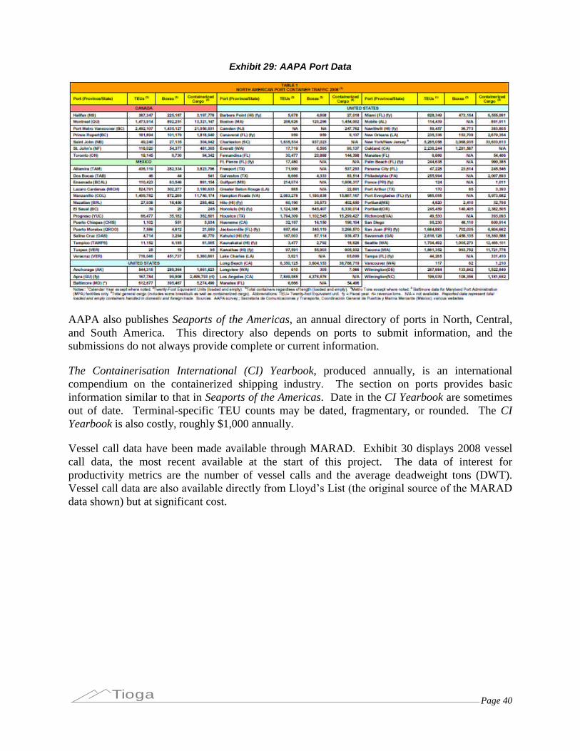
Page 40Tioga
Exhibit 29: AAPA Port Data
AAPA also publishes Seaports of the Americas, an annual directory of ports in North, Central,and South America. This directory also depends on ports to submit information, and thesubmissions do not always provide complete or current information.
The Containerisation International (CI) Yearbook, produced annually, is an internationalcompendium on the containerized shipping industry. The section on ports provides basicinformation similar to that in Seaports of the Americas. Date in the CI Yearbook are sometimesout of date. Terminal-specific TEU counts may be dated, fragmentary, or rounded. The CIYearbook is also costly, roughly $1,000 annually.
Vessel call data have been made available through MARAD. Exhibit 30 displays 2008 vesselcall data, the most recent available at the start of this project. The data of interest forproductivity metrics are the number of vessel calls and the average deadweight tons (DWT).Vessel call data are also available directly from Lloyd’s List (the original source of the MARAD data shown) but at significant cost.
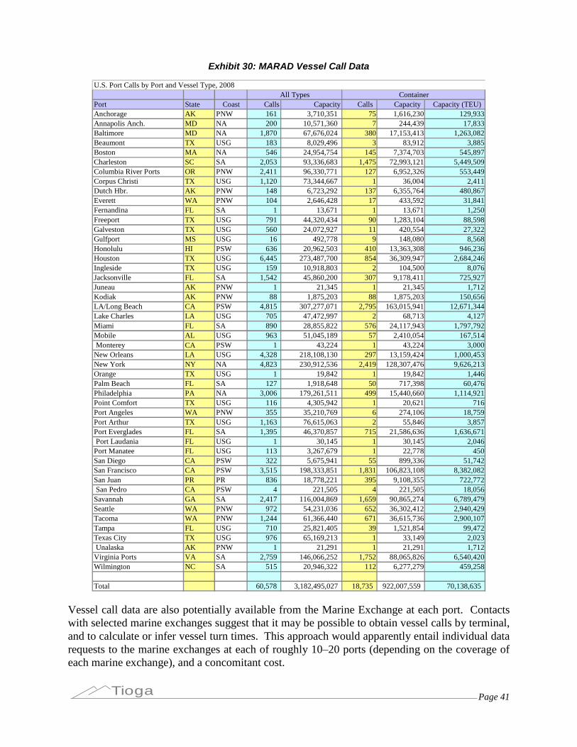
Page 41Tioga
Exhibit 30: MARAD Vessel Call Data
U.S. Port Calls by Port and Vessel Type, 2008
Port State Coast Calls Capacity Calls Capacity Capacity (TEU)Anchorage AK PNW 161 3,710,351 75 1,616,230 129,933Annapolis Anch. MD NA 200 10,571,360 7 244,439 17,833Baltimore MD NA 1,870 67,676,024 380 17,153,413 1,263,082Beaumont TX USG 183 8,029,496 3 83,912 3,885Boston MA NA 546 24,954,754 145 7,374,703 545,897Charleston SC SA 2,053 93,336,683 1,475 72,993,121 5,449,509Columbia River Ports OR PNW 2,411 96,330,771 127 6,952,326 553,449Corpus Christi TX USG 1,120 73,344,667 1 36,004 2,411Dutch Hbr. AK PNW 148 6,723,292 137 6,355,764 480,867Everett WA PNW 104 2,646,428 17 433,592 31,841Fernandina FL SA 1 13,671 1 13,671 1,250Freeport TX USG 791 44,320,434 90 1,283,104 88,598Galveston TX USG 560 24,072,927 11 420,554 27,322Gulfport MS USG 16 492,778 9 148,080 8,568Honolulu HI PSW 636 20,962,503 410 13,363,308 946,236Houston TX USG 6,445 273,487,700 854 36,309,947 2,684,246Ingleside TX USG 159 10,918,803 2 104,500 8,076Jacksonville FL SA 1,542 45,860,200 307 9,178,411 725,927Juneau AK PNW 1 21,345 1 21,345 1,712Kodiak AK PNW 88 1,875,203 88 1,875,203 150,656LA/Long Beach CA PSW 4,815 307,277,071 2,795 163,015,941 12,671,344Lake Charles LA USG 705 47,472,997 2 68,713 4,127Miami FL SA 890 28,855,822 576 24,117,943 1,797,792Mobile AL USG 963 51,045,189 57 2,410,054 167,514Monterey CA PSW 1 43,224 1 43,224 3,000
New Orleans LA USG 4,328 218,108,130 297 13,159,424 1,000,453New York NY NA 4,823 230,912,536 2,419 128,307,476 9,626,213Orange TX USG 1 19,842 1 19,842 1,446Palm Beach FL SA 127 1,918,648 50 717,398 60,476Philadelphia PA NA 3,006 179,261,511 499 15,440,660 1,114,921Point Comfort TX USG 116 4,305,942 1 20,621 716Port Angeles WA PNW 355 35,210,769 6 274,106 18,759Port Arthur TX USG 1,163 76,615,063 2 55,846 3,857Port Everglades FL SA 1,395 46,370,857 715 21,586,636 1,636,671Port Laudania FL USG 1 30,145 1 30,145 2,046
Port Manatee FL USG 113 3,267,679 1 22,778 450San Diego CA PSW 322 5,675,941 55 899,336 51,742San Francisco CA PSW 3,515 198,333,851 1,831 106,823,108 8,382,082San Juan PR PR 836 18,778,221 395 9,108,355 722,772San Pedro CA PSW 4 221,505 4 221,505 18,056
Savannah GA SA 2,417 116,004,869 1,659 90,865,274 6,789,479Seattle WA PNW 972 54,231,036 652 36,302,412 2,940,429Tacoma WA PNW 1,244 61,366,440 671 36,615,736 2,900,107Tampa FL USG 710 25,821,405 39 1,521,854 99,472Texas City TX USG 976 65,169,213 1 33,149 2,023Unalaska AK PNW 1 21,291 1 21,291 1,712
Virginia Ports VA SA 2,759 146,066,252 1,752 88,065,826 6,540,420Wilmington NC SA 515 20,946,322 112 6,277,279 459,258
Total 60,578 3,182,495,027 18,735 922,007,559 70,138,635
All Types Container
Vessel call data are also potentially available from the Marine Exchange at each port. Contactswith selected marine exchanges suggest that it may be possible to obtain vessel calls by terminal,and to calculate or infer vessel turn times. This approach would apparently entail individual datarequests to the marine exchanges at each of roughly 10–20 ports (depending on the coverage ofeach marine exchange), and a concomitant cost.

Page 42Tioga
Data associated with operating costs or rates are highly sensitive, and will remain so. Marineterminal operators negotiate rates and terms of service with their ocean carrier customers. Thoserates are embodied in confidential contracts, just as with many businesses.
Labor data of any kind are highly sensitive and considered proprietary. The wage rates, benefits,and work rules of the longshoreman’s union (ILA on the East Coast, ILWU on the West Coast)are highly complex and not easily understood. These rules and contract terms lead to situationsthat are embarrassing to terminal operators, such as paying workers who actually stay home andhiring several more workers than are actually needed for the job. Revelation of these practicesfrequently leads to indignation among ocean carriers and customers.
Employer’s organizations (e.g., the Pacific Maritime Association on the West Coast) helpadminister the Longshore contracts and retain data on hours worked, wages paid, etc. These dataare available in aggregate on association websites, but are not presented in a way that wouldallow analysts to distinguish labor at a container terminal from labor at other port operations withthe same job classifications.
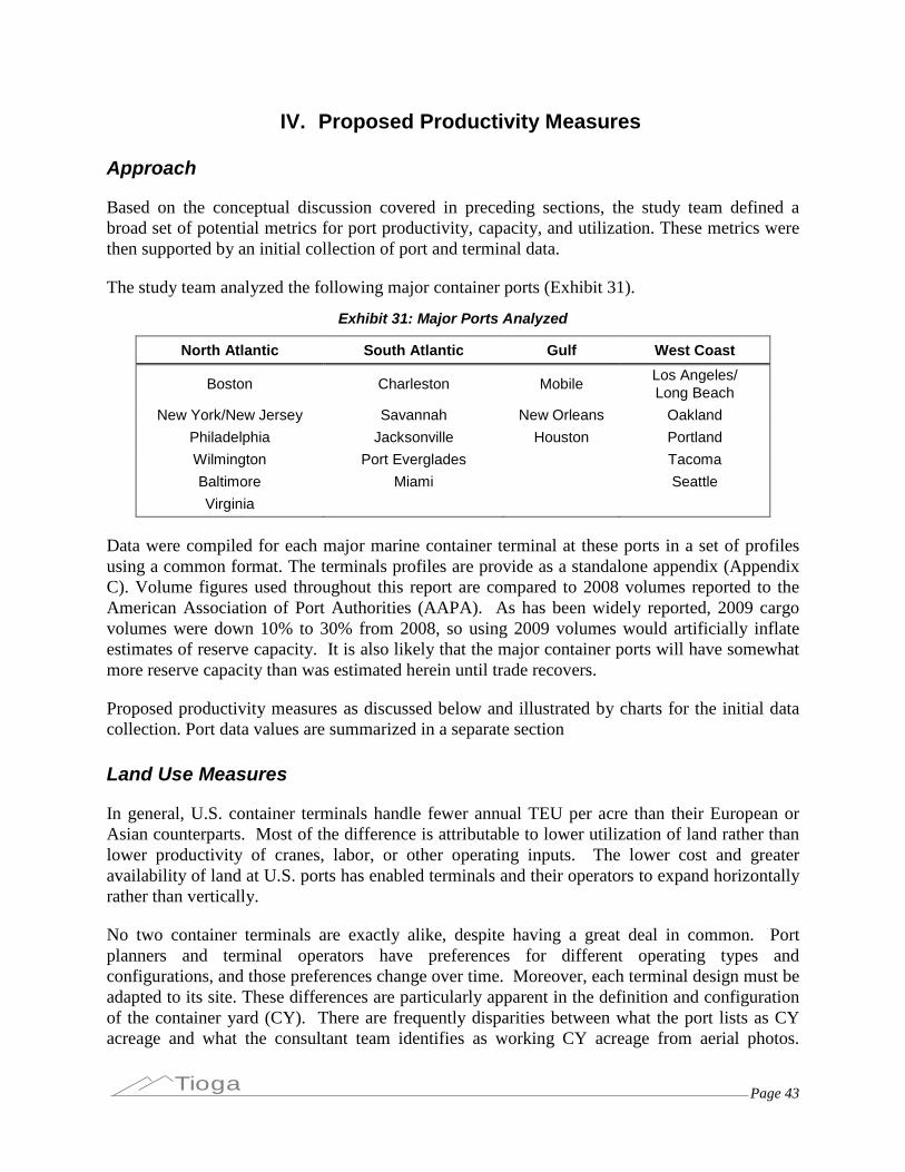
Page 43Tioga
IV. Proposed Productivity Measures
Approach
Based on the conceptual discussion covered in preceding sections, the study team defined abroad set of potential metrics for port productivity, capacity, and utilization. These metrics werethen supported by an initial collection of port and terminal data.
The study team analyzed the following major container ports (Exhibit 31).
Exhibit 31: Major Ports Analyzed
North Atlantic South Atlantic Gulf West Coast
Boston Charleston Mobile Los Angeles/Long Beach
New York/New Jersey Savannah New Orleans OaklandPhiladelphia Jacksonville Houston PortlandWilmington Port Everglades TacomaBaltimore Miami SeattleVirginia
Data were compiled for each major marine container terminal at these ports in a set of profilesusing a common format. The terminals profiles are provide as a standalone appendix (AppendixC). Volume figures used throughout this report are compared to 2008 volumes reported to theAmerican Association of Port Authorities (AAPA). As has been widely reported, 2009 cargovolumes were down 10% to 30% from 2008, so using 2009 volumes would artificially inflateestimates of reserve capacity. It is also likely that the major container ports will have somewhatmore reserve capacity than was estimated herein until trade recovers.
Proposed productivity measures as discussed below and illustrated by charts for the initial datacollection. Port data values are summarized in a separate section
Land Use Measures
In general, U.S. container terminals handle fewer annual TEU per acre than their European orAsian counterparts. Most of the difference is attributable to lower utilization of land rather thanlower productivity of cranes, labor, or other operating inputs. The lower cost and greateravailability of land at U.S. ports has enabled terminals and their operators to expand horizontallyrather than vertically.
No two container terminals are exactly alike, despite having a great deal in common. Portplanners and terminal operators have preferences for different operating types andconfigurations, and those preferences change over time. Moreover, each terminal design must beadapted to its site. These differences are particularly apparent in the definition and configurationof the container yard (CY). There are frequently disparities between what the port lists as CYacreage and what the consultant team identifies as working CY acreage from aerial photos.

Page 44Tioga
Depending on local practice, land used for chassis storage, land used for equipment maintenance,or land not presently used at all may or may not be included as CY acreage. The study teamfocused on land being used for container storage, so the figures in this report tend to beconservative.
While the inputs of all terminal types can be generalized as land capital, and labor, data oncapital investment and labor man-hours are hard to come by. The issue of land is complicated bythe difference between gross and net terminal acres, and because port terminal land is rarelyvalued at market prices.
CY/Gross Ratio
The first major distinction is between gross acres and CY acres. The study team analyzed theuse of space in major U.S. container terminals to distinguish between gross and net acreage, andto develop more accurate and meaningful productivity measures. The ratio of CY acres to total(gross) acres (Exhibit 32) helps characterize a port’s land-use pattern and shed light on theinterpretation of other metrics. Ports and terminals with on-dock rail will have lower ratios, aswill legacy or combination terminals that include non-container functions.
Exhibit 32: CY/Gross Acreage Ratio
49%
59%
29%
50%
42%
34%
43% 41%
33%
72%
58%62% 63% 62%
58%
38%
56% 57%52%
50%48% 50%
45%
48%
85%
0%
10%
20%
30%
40%
50%
60%
70%
80%
90%
Boston
NYNJ
Delawar
e River
Baltim
oreVPA
APMPorts
mouth
N. Atla
nticPorts
Charles
ton
Savan
nah
Jack
sonvil
le
PortEve
rglad
es
Miami
S. Atla
nticPorts
Mobile
NewOrle
ans
Houston
GulfPorts
East &
GulfCoas
t PortsLALB
Oaklan
d
Portlan
d
Seattl
e
Tacom
a
Wes
t Coast Ports
U.S. M
ainlan
dPorts
U.S. container ports are frequently compared with ports in Hong Kong, Singapore, Rotterdam,and others on the basis of annual TEU per acre. U.S. ports invariably compare poorly. Yet U.S.container ports have lower annual TEU per acre not necessarily because they make poor use ofavailable space, but because they have more space to handle the available cargo.
Most foreign terminals use over 75% of their space as container yard. In the US, the average is49%. Exhibit 33 shows Seagirt in Baltimore, which is fairly typical.
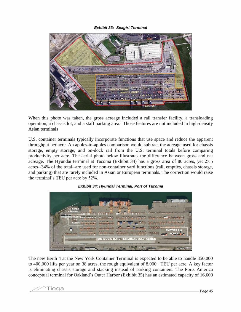
Page 45Tioga
Exhibit 33: Seagirt Terminal
When this photo was taken, the gross acreage included a rail transfer facility, a transloadingoperation, a chassis lot, and a staff parking area. Those features are not included in high-densityAsian terminals
U.S. container terminals typically incorporate functions that use space and reduce the apparentthroughput per acre. An apples-to-apples comparison would subtract the acreage used for chassisstorage, empty storage, and on-dock rail from the U.S. terminal totals before comparingproductivity per acre. The aerial photo below illustrates the difference between gross and netacreage. The Hyundai terminal at Tacoma (Exhibit 34) has a gross area of 80 acres, yet 27.5acres--34% of the total--are used for non-container yard functions (rail, empties, chassis storage,and parking) that are rarely included in Asian or European terminals. The correction would raisethe terminal’s TEU per acre by 52%.
Exhibit 34: Hyundai Terminal, Port of Tacoma
ON-DOCK RAIL TERMINAL 22.0 ACRES
EMPTIES 2.6ACRES
CHASSIS1.5
ACRES
1.4 ACRESPARKING
The new Berth 4 at the New York Container Terminal is expected to be able to handle 350,000to 400,000 lifts per year on 38 acres, the rough equivalent of 8,000+ TEU per acre. A key factoris eliminating chassis storage and stacking instead of parking containers. The Ports Americaconceptual terminal for Oakland’s Outer Harbor (Exhibit 35) has an estimated capacity of 16,600
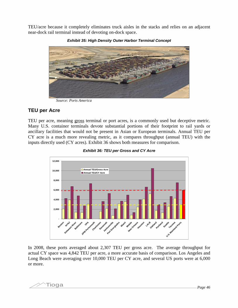
Page 46Tioga
TEU/acre because it completely eliminates truck aisles in the stacks and relies on an adjacentnear-dock rail terminal instead of devoting on-dock space.
Exhibit 35: High Density Outer Harbor Terminal Concept
Source: Ports America
TEU per Acre
TEU per acre, meaning gross terminal or port acres, is a commonly used but deceptive metric.Many U.S. container terminals devote substantial portions of their footprint to rail yards orancillary facilities that would not be present in Asian or European terminals. Annual TEU perCY acre is a much more revealing metric, as it compares throughput (annual TEU) with theinputs directly used (CY acres). Exhibit 36 shows both measures for comparison.
Exhibit 36: TEU per Gross and CY Acre
-
2,000
4,000
6,000
8,000
10,000
12,000
Boston
NYNJ
Delawar
e River
Baltim
oreVPA
APMPorts
mouth
Charles
ton
Savan
nah
Jack
sonvil
le
PortEve
rglad
es
Miami
Mobile
NewOrle
ans
Houston
LALB
Oaklan
d
Portlan
d
Seattl
e
Tacom
a
U.S. M
ainlan
dPorts
Annual TEU/Gross AcreAnnual TEU/CY Acre
In 2008, these ports averaged about 2,307 TEU per gross acre. The average throughput foractual CY space was 4,842 TEU per acre, a more accurate basis of comparison. Los Angeles andLong Beach were averaging over 10,000 TEU per CY acre, and several US ports were at 6,000or more.
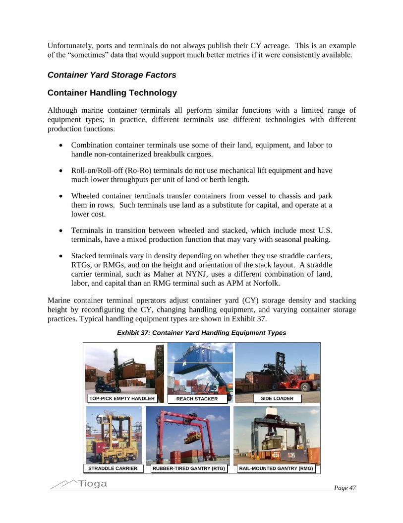
Page 47Tioga
Unfortunately, ports and terminals do not always publish their CY acreage. This is an exampleof the “sometimes” data that would support much better metrics if it were consistently available.
Container Yard Storage Factors
Container Handling Technology
Although marine container terminals all perform similar functions with a limited range ofequipment types; in practice, different terminals use different technologies with differentproduction functions.
Combination container terminals use some of their land, equipment, and labor tohandle non-containerized breakbulk cargoes.
Roll-on/Roll-off (Ro-Ro) terminals do not use mechanical lift equipment and havemuch lower throughputs per unit of land or berth length.
Wheeled container terminals transfer containers from vessel to chassis and parkthem in rows. Such terminals use land as a substitute for capital, and operate at alower cost.
Terminals in transition between wheeled and stacked, which include most U.S.terminals, have a mixed production function that may vary with seasonal peaking.
Stacked terminals vary in density depending on whether they use straddle carriers,RTGs, or RMGs, and on the height and orientation of the stack layout. A straddlecarrier terminal, such as Maher at NYNJ, uses a different combination of land,labor, and capital than an RMG terminal such as APM at Norfolk.
Marine container terminal operators adjust container yard (CY) storage density and stackingheight by reconfiguring the CY, changing handling equipment, and varying container storagepractices. Typical handling equipment types are shown in Exhibit 37.
Exhibit 37: Container Yard Handling Equipment Types
TOP-PICK EMPTY HANDLERTOP-PICK EMPTY HANDLER REACH STACKERREACH STACKER SIDE LOADERSIDE LOADER
STRADDLE CARRIERSTRADDLE CARRIER RUBBER-TIRED GANTRY (RTG)RUBBER-TIRED GANTRY (RTG) RAIL-MOUNTED GANTRY (RMG)RAIL-MOUNTED GANTRY (RMG)
TOP-PICK EMPTY HANDLERTOP-PICK EMPTY HANDLER REACH STACKERREACH STACKER SIDE LOADERSIDE LOADER
STRADDLE CARRIERSTRADDLE CARRIER RUBBER-TIRED GANTRY (RTG)RUBBER-TIRED GANTRY (RTG) RAIL-MOUNTED GANTRY (RMG)RAIL-MOUNTED GANTRY (RMG)

Page 48Tioga
Exhibit 38 displays the progression of terminal handling methods from lowest to highest density.Virtually all U.S. marine container terminals use a mix of the handling methods shown in Exhibit37 and Exhibit 38, and vary that mix to provide sufficient capacity at minimum cost. Terminaloperators gravitate to low-density, low-cost operating methods whenever possible.
Exhibit 38: Progression of Terminal Handling Methods
DENSITY TYPE COMMENT
Ro/Ro or Ship’s gear Very small, barge, specialized
Wheeled Combination Small, mixed, legacy
Dedicated Wheeled Older terminals when new
Wheeled/Top-pick Transition temrinals
Top-pick/Wheeled Transition temrinals
Straddle/Top-pick/Wheeled Hybrid terminal
RTG/Top-pick/Wheeled Dominant hyrbid typeStraddle Carrier NIT Virginia
RTG No US Example
VERY HIGH DENSITY Pure RMG APM Portsmouth
VERY LOW DENSITY
LOW DENSITY
MID DENSITY
HIGH DENSITY
Faced with a need to accommodate more trade, terminals move progressively up the densityscale.
Terminal operators start increasing density by stacking empty containers insteadof leaving them parked on chassis. Empties can be handled with inexpensiveequipment and stacked first-in/last-out since they are largely interchangeable.
As additional capacity is required, terminal operators begin stacking loadedexport containers. Export containers typically build up over the week prior tovessel arrival and need not be accessed until it is time to load that vessel. Loadedcontainers are heavier than empties, however, and must be accessed in a sequencetied to vessel loading plans. Loaded export storage, therefore, usually requiresmore expensive RTGs or straddle carriers.
Terminal operators typically leave loaded import containers parked on chassis(“wheeled”) as long as possible to both minimize handling cost and maximize responsiveness to customer needs. When loaded imports are eventually stacked,they require RTG or straddle carriers for flexible access.
Containers with special requirements are rarely stacked, and most terminalsreserve space to keep such movements on chassis. Specialized movementsinclude refrigerated containers, containers with hazardous cargo, over-size orover-weight containers, tank containers, and containers held for CBP inspection.
A wheeled operation in which all containers in the terminal are placed on chassis is the lowestdensity and most economical operating system. Such an operation requires much more land forparked chassis with and without containers than a stacked system. Yard lift equipment is onlyrequired to move containers off the wrong chassis and onto the right one, or to handle containersfor maintenance and repair.
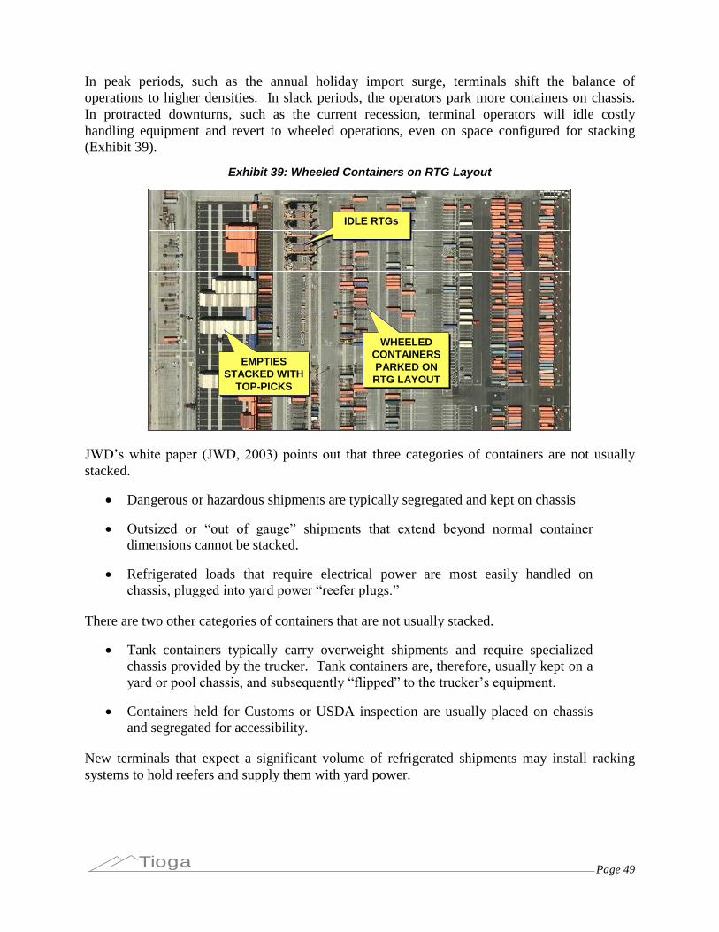
Page 49Tioga
In peak periods, such as the annual holiday import surge, terminals shift the balance ofoperations to higher densities. In slack periods, the operators park more containers on chassis.In protracted downturns, such as the current recession, terminal operators will idle costlyhandling equipment and revert to wheeled operations, even on space configured for stacking(Exhibit 39).
Exhibit 39: Wheeled Containers on RTG Layout
IDLE RTGsIDLE RTGs
EMPTIESSTACKED WITH
TOP-PICKS
EMPTIESSTACKED WITH
TOP-PICKS
WHEELEDCONTAINERSPARKED ONRTG LAYOUT
WHEELEDCONTAINERSPARKED ONRTG LAYOUT
IDLE RTGsIDLE RTGs
EMPTIESSTACKED WITH
TOP-PICKS
EMPTIESSTACKED WITH
TOP-PICKS
WHEELEDCONTAINERSPARKED ONRTG LAYOUT
WHEELEDCONTAINERSPARKED ONRTG LAYOUT
JWD’s white paper (JWD, 2003) points out that three categories of containers are not usuallystacked.
Dangerous or hazardous shipments are typically segregated and kept on chassis
Outsized or “out of gauge” shipments that extend beyond normal container dimensions cannot be stacked.
Refrigerated loads that require electrical power are most easily handled onchassis, plugged into yard power “reefer plugs.”
There are two other categories of containers that are not usually stacked.
Tank containers typically carry overweight shipments and require specializedchassis provided by the trucker. Tank containers are, therefore, usually kept on ayard or pool chassis, and subsequently “flipped” to the trucker’s equipment.
Containers held for Customs or USDA inspection are usually placed on chassisand segregated for accessibility.
New terminals that expect a significant volume of refrigerated shipments may install rackingsystems to hold reefers and supply them with yard power.
Page 50Tioga
Terminal Types and Moves per Box
Each terminal handling method leads to different average moves per container. Wheeledoperations are generally preferred in large part because they require only one container lift. Thenumber of lifts, operating cost, and complexity grow as density increases.
Wheeled–One lift per box
- Vessel to highway chassis
Stacked–Three+ lifts per box
- Vessel to yard chassis
- Yard chassis to stack
- Stack to highway chassis (potential stack sorting)
Straddle Carrier–Two lifts per box
- Vessel to stack/row
- Stack/row to highway chassis (minimal row sorting)
Wheeled operations are more labor- and capital-efficient, and average moves per box is anindicator of efficiency and cost. While average moves per box would be a strong indicator ofunderlying cost, such data require data-links between mobile lift equipment and the terminal’s operating system. Even where such links are in place, the data are difficult to collect andanalyze, and would be highly confidential.
CY Capacity and Productivity Estimates
The CY capacity and productivity estimation method used in this study is necessarily acompromise, based on a “snapshot” of current stacking density. The team used the most recentaerial photos available on Google Earth and estimated the CY acreage configured for eachstorage density category. The precision of this method is limited in several respects.
The latest available aerial photos vary from a few months old to 2 to 3 years old,and terminal configurations and uses can change on short notice.
Aerial estimates of acreage and uses are imprecise, although probably sufficientlyaccurate for high-level capacity estimates.
The container yard capacities were estimated by dividing the CY acreage by handling type andapplying the storage factors for each to derive estimated TEU slot totals. The typical storagedensities for terminal handling methods are shown in Exhibit 40.
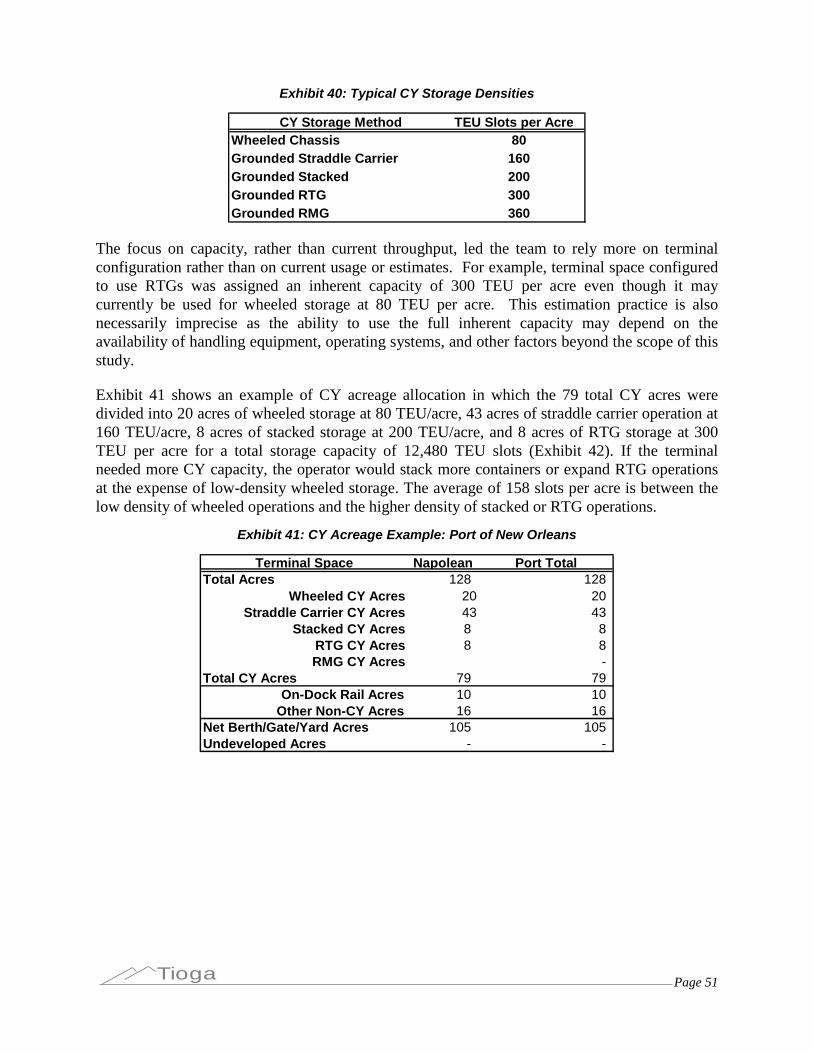
Page 51Tioga
Exhibit 40: Typical CY Storage Densities
CY Storage Method TEU Slots per AcreWheeled Chassis 80Grounded Straddle Carrier 160Grounded Stacked 200Grounded RTG 300Grounded RMG 360
The focus on capacity, rather than current throughput, led the team to rely more on terminalconfiguration rather than on current usage or estimates. For example, terminal space configuredto use RTGs was assigned an inherent capacity of 300 TEU per acre even though it maycurrently be used for wheeled storage at 80 TEU per acre. This estimation practice is alsonecessarily imprecise as the ability to use the full inherent capacity may depend on theavailability of handling equipment, operating systems, and other factors beyond the scope of thisstudy.
Exhibit 41 shows an example of CY acreage allocation in which the 79 total CY acres weredivided into 20 acres of wheeled storage at 80 TEU/acre, 43 acres of straddle carrier operation at160 TEU/acre, 8 acres of stacked storage at 200 TEU/acre, and 8 acres of RTG storage at 300TEU per acre for a total storage capacity of 12,480 TEU slots (Exhibit 42). If the terminalneeded more CY capacity, the operator would stack more containers or expand RTG operationsat the expense of low-density wheeled storage. The average of 158 slots per acre is between thelow density of wheeled operations and the higher density of stacked or RTG operations.
Exhibit 41: CY Acreage Example: Port of New Orleans
Terminal Space Napolean Port TotalTotal Acres 128 128
Wheeled CY Acres 20 20Straddle Carrier CY Acres 43 43
Stacked CY Acres 8 8RTG CY Acres 8 8RMG CY Acres -
Total CY Acres 79 79On-Dock Rail Acres 10 10
Other Non-CY Acres 16 16Net Berth/Gate/Yard Acres 105 105Undeveloped Acres - -

Page 52Tioga
Exhibit 42: CY Capacity Example: Port of New Orleans
Container Yard Capacity Napolean Port TotalWheeled Chassis Slots 1,600 1,600Grounded Straddle Carrier Slots 6,880 6,880Grounded Stacked Slots 1,600 1,600Grounded RTG Slots 2,400 2,400Grounded RMG Slots - -TEU Storage Slots 12,480 12,480Avg TEU Slots/CY Acre 158 158Maximum Annual Slot Turnover 70.0 70.0Maximum Annual CY TEU Capacity 873,600 873,600Sustainable CY TEU Capacity @ 80% 698,880 698,8802008 Annual TEU 313,765 313,7652008 TEU per CY Slot 25 252008 CY Capacity Utilization 45% 45%
As Exhibit 42 shows, the team estimated the maximum annual TEU capacity based on amaximum annual slot turnover of 70 turns annually, an aggressive average of more than one turnper week and equivalent to an average container dwell time of slightly over 5 days. Whiletheoretically possible, particularly in periods of peak demand, operation at this level of intensityis unlikely to be sustainable day-in and day-out. Moreover, if this level of density were routine,there would be no reserve capacity to handle the inevitable trade surges. The study team,therefore, also estimated sustainable CY TEU capacity at 80% of the maximum, following acommon industry rule-of-thumb. There is only one major container terminal at the Port of NewOrleans, so, in the examples above, the port total is the same as the Napoleon terminal total.
2008 annual TEU counts were compared with the estimated sustainable TEU capacity toestimate the annual TEU per storage slot (25 in the example) and average annual CY capacityutilization (45% in the example).
Under greater pressure, such as was experienced in Southern California before the currentrecession, marine terminals can also increase capacity by reducing container dwell times. Byshortening “free time” allowances and raising or vigorously enforcing charges for excess dwell time, terminal operators have succeeded in reducing dwell times for import loads, thus,increasing storage turnover. On the export side, terminals can limit the time in advance of vesselarrival during which export containers will be accepted. To reduce the dwell time of emptycontainers, terminal operators and their ocean carrier clients can move empties to off-terminaldepots or return leased containers to leasing company depots.
TEU Storage Slots (CY Slot Capacity)
The total TEU storage slots in a terminal or port reflects the combination of CY acreage and theCY operating methods in use, and characterizes static storage capacity (Exhibit 43). There aretwo factors at play: CY acreage and stacking density. The combination highlights the enormoustotal capacity at the Ports of Los Angeles and Long Beach. Were Seattle and Tacoma combinedin the data, the combination would look much larger than the two individual ports.

Page 53Tioga
Exhibit 43: TEU Storage Slots
11,900
125,320
15,000
44,660
23,700
55,180
12,480
243,180
72,980
12,320
40,18041,400
23,080
47,040 42,140
129,260
55,840
16,040
117,960
-
50,000
100,000
150,000
200,000
250,000
Boston
NYNJ
Delawar
e River
Baltim
oreVPA
APMPorts
mouth
Charles
ton
Savan
nah
Jack
sonvil
le
PortEve
rglad
es
Miami
Mobile
NewOrle
ans
Houston
LALB
Oaklan
d
Portlan
d
Seattl
e
Tacom
a
TEU Slots per CY Acre (Storage Density)
TEU slots per acre is a useful measure of CY capacity because it captures the impact of stackingheight and technology as well as acreage. US ports average about 190 slots per acre, roughlyhalf way between an all-wheeled terminal at 80 to 100 TEU per acre and an all-RTG terminal at300 per acre. Almost every US terminal actually has a mix of wheeled, top-pick, and RTGoperations. These numbers also indicate substantial room for growth through greater density.
Storage density is a mid-point in the analysis of capacity and productivity. Storage density(Exhibit 44) reflects the way the terminal space has been allocated among various storagetechnologies. A higher number indicates that the facility has been configured for high annualthroughput, but does not reflect the extent to which that capacity is being used.
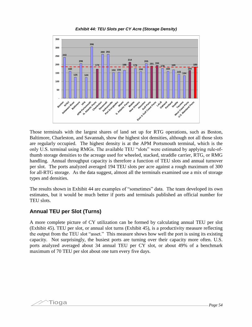
Page 54Tioga
Exhibit 44: TEU Slots per CY Acre (Storage Density)
243
160
125
206
124
306
260 261
153 155
214
158
205191 194
178160
143134
185169
165176166174
-
50
100
150
200
250
300
350
Boston
NYNJ
Delawar
e River
Baltim
oreVPA
APMPorts
mouth
N. Atla
nticPorts
Charles
ton
Savan
nah
Jack
sonvil
le
PortEve
rglad
es
Miami
S. Atla
nticPorts
Mobile
NewOrle
ans
Houston
GulfPorts
East &
GulfCoas
t PortsLALB
Oaklan
d
Portlan
d
Seattl
e
Tacom
a
Wes
t Coast Ports
U.S. M
ainlan
dPorts
Those terminals with the largest shares of land set up for RTG operations, such as Boston,Baltimore, Charleston, and Savannah, show the highest slot densities, although not all those slotsare regularly occupied. The highest density is at the APM Portsmouth terminal, which is theonly U.S. terminal using RMGs. The available TEU “slots” were estimated by applying rule-of-thumb storage densities to the acreage used for wheeled, stacked, straddle carrier, RTG, or RMGhandling. Annual throughput capacity is therefore a function of TEU slots and annual turnoverper slot. The ports analyzed averaged 194 TEU slots per acre against a rough maximum of 300for all-RTG storage. As the data suggest, almost all the terminals examined use a mix of storagetypes and densities.
The results shown in Exhibit 44 are examples of “sometimes” data. The teamdeveloped its ownestimates, but it would be much better if ports and terminals published an official number forTEU slots.
Annual TEU per Slot (Turns)
A more complete picture of CY utilization can be formed by calculating annual TEU per slot(Exhibit 45). TEU per slot, or annual slot turns (Exhibit 45), is a productivity measure reflectingthe output from the TEU slot “asset.” This measure shows how well the port is using its existingcapacity. Not surprisingly, the busiest ports are turning over their capacity more often. U.S.ports analyzed averaged about 34 annual TEU per CY slot, or about 49% of a benchmarkmaximum of 70 TEU per slot about one turn every five days.
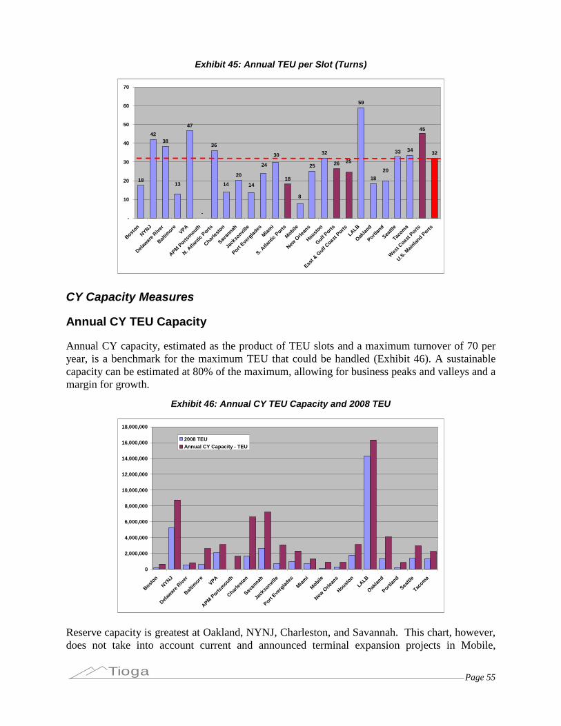
Page 55Tioga
Exhibit 45: Annual TEU per Slot (Turns)
18
4238
47
-
2018
25
32
26
59
18
33 34 32
14
24
13
25
14
20
45
8
30
36
-
10
20
30
40
50
60
70
Boston
NYNJ
Delawar
e River
Baltim
oreVPA
APMPorts
mouth
N. Atla
nticPorts
Charles
ton
Savan
nah
Jack
sonvil
le
PortEve
rglad
es
Miami
S. Atla
nticPorts
Mobile
NewOrle
ans
Houston
GulfPorts
East &
GulfCoas
t PortsLALB
Oaklan
d
Portlan
d
Seattl
e
Tacom
a
Wes
t Coast Ports
U.S. M
ainlan
dPorts
CY Capacity Measures
Annual CY TEU Capacity
Annual CY capacity, estimated as the product of TEU slots and a maximum turnover of 70 peryear, is a benchmark for the maximum TEU that could be handled (Exhibit 46). A sustainablecapacity can be estimated at 80% of the maximum, allowing for business peaks and valleys and amargin for growth.
Exhibit 46: Annual CY TEU Capacity and 2008 TEU
0
2,000,000
4,000,000
6,000,000
8,000,000
10,000,000
12,000,000
14,000,000
16,000,000
18,000,000
Boston
NYNJ
Delawar
e River
Baltim
oreVPA
APMPorts
mouth
Charles
ton
Savan
nah
Jack
sonvil
le
PortEve
rglad
es
Miami
Mobile
NewOrle
ans
Houston
LALB
Oaklan
d
Portlan
d
Seattl
e
Tacom
a
2008 TEUAnnual CY Capacity - TEU
Reserve capacity is greatest at Oakland, NYNJ, Charleston, and Savannah. This chart, however,does not take into account current and announced terminal expansion projects in Mobile,

Page 56Tioga
Houston, and elsewhere. In terms of shear size LALB, PANYNJ, Charleston, Savannah, andJacksonville are the largest ports. The Delaware River Ports include Philadelphia andWilmington, DE. The Port of Virginia includes Norfolk, Newport News, and Portsmouthterminals.
CY Capacity Utilization
Annual TEU divided by estimated annual TEU capacity (throughput as a percentage of capacity)is a measure of CY capacity utilization. The ports shown in Exhibit 47 average 50% CY capacityutilization.
Exhibit 47: CY Capacity Utilization
31%
75%
68%
23%
83%
0%
55%
25%
36%
24%
42%
53%
32%
14%
45%
57%
46%41%
88%
33%36%
58% 60%
70%
53%
0%
10%
20%
30%
40%
50%
60%
70%
80%
90%
100%
Boston
NYNJ
Delawar
e River
Baltim
oreVPA
APMPorts
mouth
N. Atla
nticPorts
Charles
ton
Savan
nah
Jack
sonvil
le
PortEve
rglad
es
Miami
S. Atla
nticPorts
Mobile
NewOrle
ans
Houston
GulfPorts
East &
GulfCoas
t PortsLALB
Oaklan
d
Portlan
d
Seattl
e
Tacom
a
Wes
t Coast Ports
U.S. M
ainlan
dPorts
Container Crane Measures
Crane utilization metrics present a dilemma. Crane utilization and productivity can be measuredin TEU and number of vessels worked.
Terminals usually have 2-3 cranes per berth.
They can use up to 5 cranes for large vessels, so they move cranes as needed.
Most cannot handle multiple large vessels with high discharge/load volumessimultaneously.
Crane efficiency is measured in moves per working hour, a figure that is notalways made available.
There is inherent tension in this approach:
Annual crane output is higher if fewer cranes work the vessels.
Vessel turns are faster and more reliable if more cranes are used.
Page 57Tioga
Terminals can maximize crane productivity by using as few cranes as possible, but, by doingthis, risk vessel delays. Vessels cost a lot more than cranes, and the primary terminal task isturning the vessel
Crane utilization and productivity can be measured in TEU and vessels worked.
Crane efficiency would be measured in moves/hour, but data are seldomavailable.
There is a critical tradeoff. Annual crane output is higher if fewer cranes work the vessels, yetvessel turns are faster and more reliable with more cranes
The ability to handle a given vessel size depends on the berth length and draft available at theterminal. The ability to handle the cargo from that vessel depends on the number of cranesavailable, the hourly throughput capability of those cranes, and the hours those cranes areavailable in a day or week.
The primary goal of terminal operators is to service the vessel on schedule and at minimum cost.The number of cranes installed and used is determined primarily by the need to turn the vessel,with annual crane productivity a secondary consideration. This set of priorities results inrelatively low container crane utilization, as suggested by the exhibits that follow. A vessel is farmore costly to own and operate than the cranes that serve it, so crane utilization is effectivelysacrificed to vessel utilization.
The following metrics tell more in combination than separately.
Average Cranes per Berth
A typical marine terminal, such as the one shown in Exhibit 48, might have two berths and fourcranes. This configuration gives the terminal operator the flexibility to assign from one to fourcranes to a vessel, as required. as the vessel discharge and load averages increase, the number ofcranes may limit the number of vessels that can be handled simultaneously, and thereforeannually. As this limit is approached, the port or terminal operator will add cranes.

Page 58Tioga
Exhibit 48: Typical Two-Berth/Four-Crane Terminal
This arrangement lets the stevedore work two small ships at once, or put 3 to 4 cranes againstone larger or more heavily loaded ship.
Exhibit 49 shows that the U.S. average is 2.2 cranes per berth and that ports average anywhereform 1.0 to 4.0. Behind the numbers are some important differences. Both Port Everglades andOakland have lower averages, but Oakland is 4 times the size of Port Everglades. Houston andPortland have high averages, but Houston is 3 times larger than Portland.
Exhibit 49: Average Cranes per Berth
3.2
1.6 1.6
2.8
1.5
2.6
1.6
1.0
2.4
2.7
1.5
2.8
2.0
1.8
2.02.1
2.1 2.12.2 2.2
4.0
2.4
1.31.3
2.4
0.0
0.5
1.0
1.5
2.0
2.5
3.0
3.5
4.0
Boston
NYNJ
Delawar
e River
Baltim
oreVPA
APMPorts
mouth
N. Atla
nticPorts
Charles
ton
Savan
nah
Jack
sonvil
le
PortEve
rglad
es
Miami
S. Atla
nticPorts
Mobile
NewOrle
ans
Houston
GulfPorts
East &
GulfCoas
t PortsLALB
Oaklan
d
Portlan
d
Seattl
e
Tacom
a
Wes
t Coast Ports
U.S. M
ainlan
dPorts
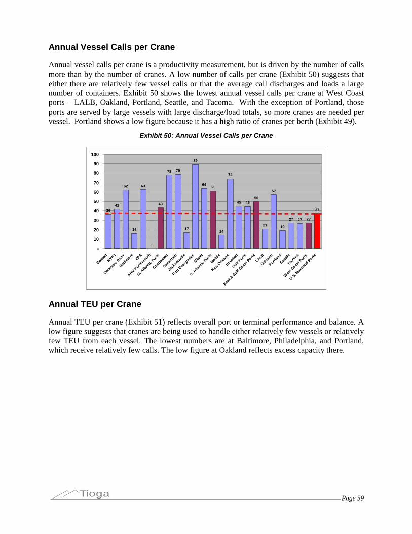
Page 59Tioga
Annual Vessel Calls per Crane
Annual vessel calls per crane is a productivity measurement, but is driven by the number of callsmore than by the number of cranes. A low number of calls per crane (Exhibit 50) suggests thateither there are relatively few vessel calls or that the average call discharges and loads a largenumber of containers. Exhibit 50 shows the lowest annual vessel calls per crane at West Coastports –LALB, Oakland, Portland, Seattle, and Tacoma. With the exception of Portland, thoseports are served by large vessels with large discharge/load totals, so more cranes are needed pervessel. Portland shows a low figure because it has a high ratio of cranes per berth (Exhibit 49).
Exhibit 50: Annual Vessel Calls per Crane
3642
62
16
63
-
43
78 79
17
89
6461
14
74
45 4550
21
57
19
27 27 27
37
-
10
20
30
40
50
60
70
80
90
100
Boston
NYNJ
Delawar
e River
Baltim
oreVPA
APMPorts
mouth
N. Atla
nticPorts
Charles
ton
Savan
nah
Jack
sonvil
le
PortEve
rglad
es
Miami
S. Atla
nticPorts
Mobile
NewOrle
ans
Houston
GulfPorts
East &
GulfCoas
t PortsLALB
Oaklan
d
Portlan
d
Seattl
e
Tacom
a
Wes
t Coast Ports
U.S. M
ainlan
dPorts
Annual TEU per Crane
Annual TEU per crane (Exhibit 51) reflects overall port or terminal performance and balance. Alow figure suggests that cranes are being used to handle either relatively few vessels or relativelyfew TEU from each vessel. The lowest numbers are at Baltimore, Philadelphia, and Portland,which receive relatively few calls. The low figure at Oakland reflects excess capacity there.

Page 60Tioga
Exhibit 51: Annual TEU per Crane
52,157
90,777
71,860
38,313
74,403
-
86,081
113,745
41,908
123,137
86,704
30,451
94,437
107,803
42,124
30,682
57,354
84,035
76,709 76,12778,441
82,588
53,919
84,54578,799
-
20,000
40,000
60,000
80,000
100,000
120,000
140,000
Boston
NYNJ
Delawar
e River
Baltim
oreVPA
APMPorts
mouth
N. Atla
nticPorts
Charles
ton
Savan
nah
Jack
sonvil
le
PortEve
rglad
es
Miami
S. Atla
nticPorts
Mobile
NewOrle
ans
Houston
GulfPorts
East &
GulfCoas
t PortsLALB
Oaklan
d
Portlan
d
Seattl
e
Tacom
a
Wes
t Coast Ports
U.S. M
ainlan
dPorts
The high figures for Port Everglades are due to inclusion of ro-ro traffic in the data. Other thanthe Port Everglades anomaly, the highest crane productivities are at LALB (due to large vesselsand high discharge/load ratios) and Savannah (due to a large number of vessel calls per berth).
Vessel Measures
Container terminal throughput is limited by the size and utilization of the vessels that call. Theaverage vessel that calls at most ports discharges and loads substantially less than its fullcapacity. There are two basic reasons for this disparity.
Vessels almost invariably call at multiple U.S. ports on each voyage, and thevessel’s total cargo discharge and load is split among those ports.
Ocean carriers, like ports and terminals, offer and deploy sufficient capacity toaccommodate growth as well as current cargo volumes. Only in peak periods ofpeak years will vessels be completely full on every voyage.
Vessel Draft, DWT, and TEU Capacity
The relationship between vessel size measured in deadweight tons (DWT) and in twenty-footequivalent units (TEU) varies, especially in very large vessels (e.g. over 8,000 TEU). Todevelop a working relationship the study team assembled a database of 350+ container vessels.
Exhibit 52 shows the relationship between DWT and draft, where both data items were availablefor a given vessel.

Page 61Tioga
Exhibit 52: DWT vs. Draft
y = 9.835Ln(x) - 65.672R2 = 0.9559
30
35
40
45
50
55
60
20,000 40,000 60,000 80,000 100,000 120,000 140,000 160,000 180,000DWT
Draft (ft)
N=119
It appears that vessel designers have kept maximum drafts within boundaries, and that the largestvessels are becoming wider rather than deeper.
Vessels rarely sail at their full design draft. To do so would entail a full load of loadedcontainers, which is uncommon. USACE guidance (Exhibit 53) suggests that maximumeffective cargo capacity is typically about 95% of DWT. Applying this ratio to design draftversus sailing draft suggests that a vessel designed for 50 feet draft would, for example, usuallysail at a maximum of 47.5 feet. While not a precise relationship, this guideline was adopted forthe capacity analysis.
Exhibit 53: USACE Guidance on Cargo Capacity as a Percentage of DWT
Adjustments for Estimating Actual Vessel CapacityShort Tons of Cargo as a Percentage of Vessel DWT
Vessel DWT % Cargo to DWT<20,000 90%
20,000 to 70,000 92%70,000 to 120,000 95%
>120,000 97%Source: IWR Report 91-R-13, National Economic DevelopmentProcedures Manual, Deep-Drat Navigation, November 1991, p. 77.
Likewise, vessels rarely use the full channel depth. For safety reasons, pilot rules and commonpractice typically require a minimum of 3 feet under keel. This rule is sometimes “bent,”and itis common at some ports to “ride the tide” to gain additional clearance. Taking the long-termview again, the capacity analysis incorporates the 3-foot minimum.
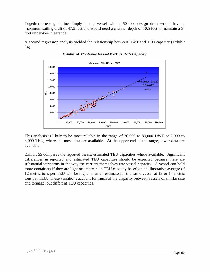
Page 62Tioga
Together, these guidelines imply that a vessel with a 50-foot design draft would have amaximum sailing draft of 47.5 feet and would need a channel depth of 50.5 feet to maintain a 3-foot under-keel clearance.
A second regression analysis yielded the relationship between DWT and TEU capacity (Exhibit54).
Exhibit 54: Container Vessel DWT vs. TEU Capacity
Container Ship TEU vs. DWT
y = 0.0838x - 253.39R2 = 0.9599
-
2,000
4,000
6,000
8,000
10,000
12,000
14,000
16,000
- 20,000 40,000 60,000 80,000 100,000 120,000 140,000 160,000 180,000
DWT
TE
U
N=353
This analysis is likely to be most reliable in the range of 20,000 to 80,000 DWT or 2,000 to6,000 TEU, where the most data are available. At the upper end of the range, fewer data areavailable.
Exhibit 55 compares the reported versus estimated TEU capacities where available. Significantdifferences in reported and estimated TEU capacities should be expected because there aresubstantial variations in the way the carriers themselves rate vessel capacity. A vessel can holdmore containers if they are light or empty, so a TEU capacity based on an illustrative average of12 metric tons per TEU will be higher than an estimate for the same vessel at 13 or 14 metrictons per TEU. These variations account for much of the disparity between vessels of similar sizeand tonnage, but different TEU capacities.
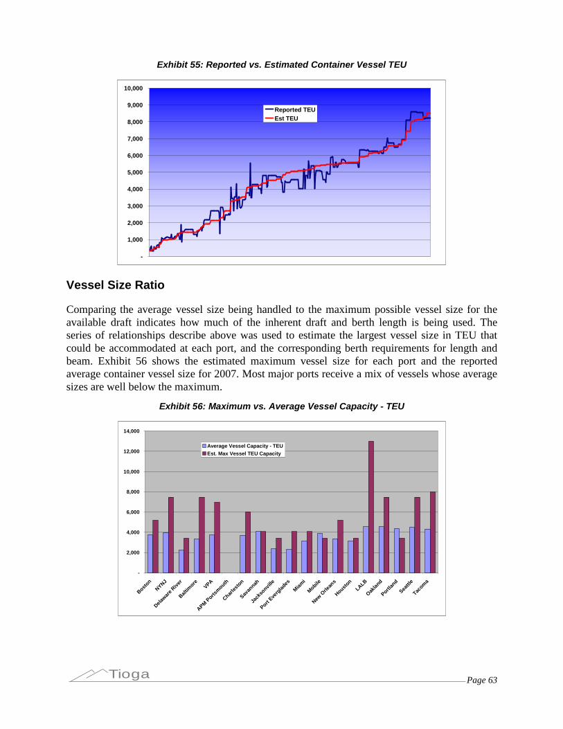
Page 63Tioga
Exhibit 55: Reported vs. Estimated Container Vessel TEU
-
1,000
2,000
3,000
4,000
5,000
6,000
7,000
8,000
9,000
10,000
Reported TEUEst TEU
Vessel Size Ratio
Comparing the average vessel size being handled to the maximum possible vessel size for theavailable draft indicates how much of the inherent draft and berth length is being used. Theseries of relationships describe above was used to estimate the largest vessel size in TEU thatcould be accommodated at each port, and the corresponding berth requirements for length andbeam. Exhibit 56 shows the estimated maximum vessel size for each port and the reportedaverage container vessel size for 2007. Most major ports receive a mix of vessels whose averagesizes are well below the maximum.
Exhibit 56: Maximum vs. Average Vessel Capacity - TEU
-
2,000
4,000
6,000
8,000
10,000
12,000
14,000
Boston
NYNJ
Delawar
e River
Baltim
oreVPA
APMPorts
mouth
Charles
ton
Savan
nah
Jack
sonvil
le
PortEve
rglad
es
Miami
Mobile
NewOrle
ans
Houston
LALB
Oaklan
d
Portlan
d
Seattl
e
Tacom
a
Average Vessel Capacity - TEUEst. Max Vessel TEU Capacity
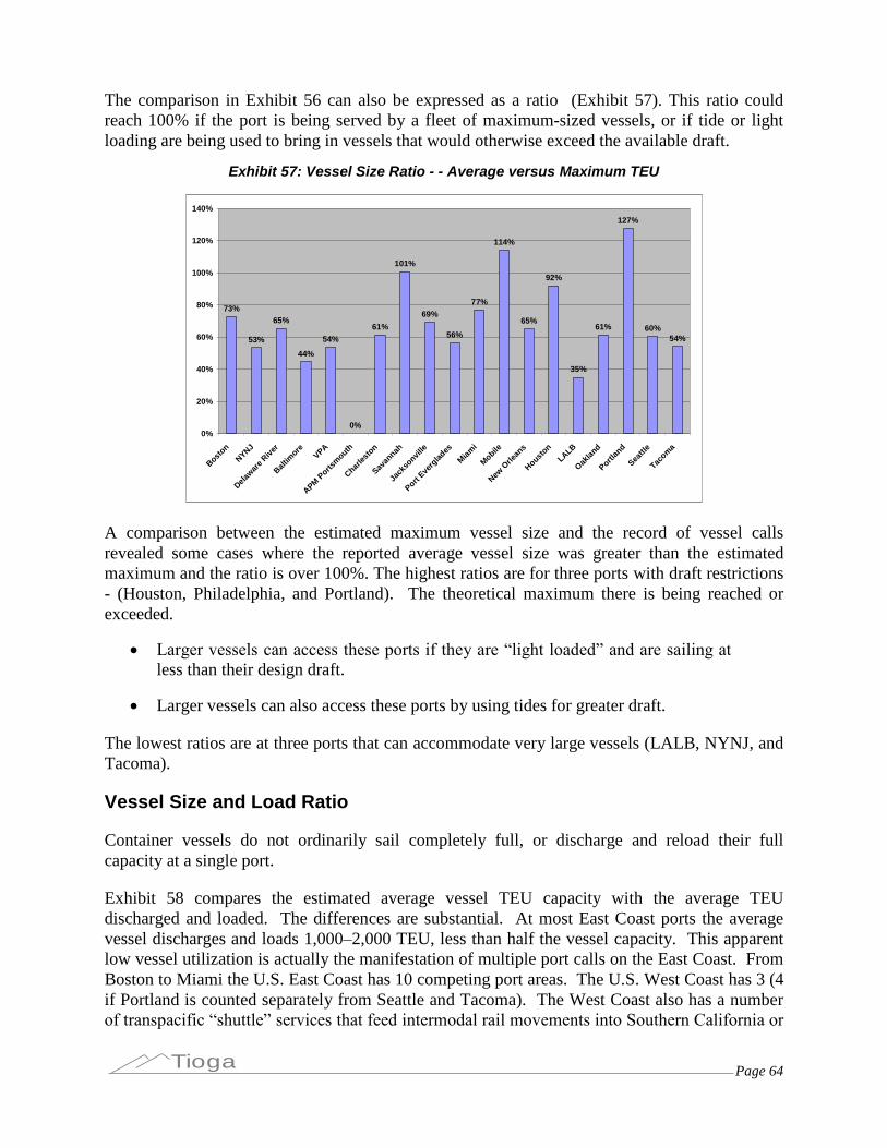
Page 64Tioga
The comparison in Exhibit 56 can also be expressed as a ratio (Exhibit 57). This ratio couldreach 100% if the port is being served by a fleet of maximum-sized vessels, or if tide or lightloading are being used to bring in vessels that would otherwise exceed the available draft.
Exhibit 57: Vessel Size Ratio - - Average versus Maximum TEU
73%
53%
65%
44%
54%
0%
61%
101%
69%
56%
77%
114%
65%
92%
35%
61%
127%
60%54%
0%
20%
40%
60%
80%
100%
120%
140%
Boston
NYNJ
Delawar
e River
Baltim
oreVPA
APMPorts
mouth
Charles
ton
Savan
nah
Jack
sonvil
le
PortEve
rglad
es
Miami
Mobile
NewOrle
ans
Houston
LALB
Oaklan
d
Portlan
d
Seattl
e
Tacom
a
A comparison between the estimated maximum vessel size and the record of vessel callsrevealed some cases where the reported average vessel size was greater than the estimatedmaximum and the ratio is over 100%. The highest ratios are for three ports with draft restrictions- (Houston, Philadelphia, and Portland). The theoretical maximum there is being reached orexceeded.
Larger vessels can access these ports if they are “light loaded” and are sailing at less than their design draft.
Larger vessels can also access these ports by using tides for greater draft.
The lowest ratios are at three ports that can accommodate very large vessels (LALB, NYNJ, andTacoma).
Vessel Size and Load Ratio
Container vessels do not ordinarily sail completely full, or discharge and reload their fullcapacity at a single port.
Exhibit 58 compares the estimated average vessel TEU capacity with the average TEUdischarged and loaded. The differences are substantial. At most East Coast ports the averagevessel discharges and loads 1,000–2,000 TEU, less than half the vessel capacity. This apparentlow vessel utilization is actually the manifestation of multiple port calls on the East Coast. FromBoston to Miami the U.S. East Coast has 10 competing port areas. The U.S. West Coast has 3 (4if Portland is counted separately from Seattle and Tacoma). The West Coast also has a numberof transpacific “shuttle” services that feed intermodal rail movements into Southern California or

Page 65Tioga
the Pacific Northwest. As the chart shows, these factors produce larger vessels loaded to agreater fraction of their capacity at West Coast ports.
Exhibit 58: Vessel Size and Load Comparison
-
1,000
2,000
3,000
4,000
5,000
6,000
Boston
NYNJ
Delawar
e River
Baltim
oreVPA
APMPorts
mouth
Charles
ton
Savan
nah
Jack
sonvil
le
PortEve
rglad
es
Miami
Mobile
NewOrle
ans
Houston
LALB
Oaklan
d
Portlan
d
Seattl
e
Tacom
a
Average Vessel Capacity - TEUAverage TEU per Vessel
As vessel sizes grew over the preceding decade, concern increased over the potential for “load centering,” the anticipated practice of using largevessels to serve large ports and smaller feedervessels (or inland truck or rail service) to serve smaller ports. The practice was not widely usedin part because carriers formed Vessel Sharing Agreements (VSAs) and alliances, and continueddirect service to small ports under competitive pressure.
The data in Exhibit 58, however, suggest that load centering or similar practices may be limitingvolumes going through Boston, Philadelphia, Baltimore, and Portland. These ports are alladjacent to major competitors. PANYNJ competes with Boston and Philadelphia; Virginiacompetes with Baltimore, and Seattle and Tacoma compete with Portland. Philadelphia,Baltimore, and Portland also have the competitive disadvantage of being located some distancefrom the open ocean.
These data can be expressed as a ratio. The theoretical maximum is 200% of vessel capacity: avessel completely emptied and reloaded. Exhibit 59 shows that most ports discharge and load anaverage of 30-40% of vessel capacity. The exceptions are Houston, the dominant port in theGulf, and LALB.
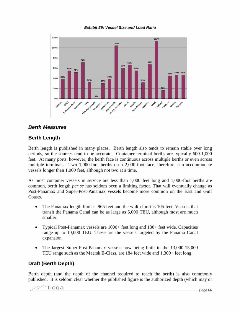
Page 66Tioga
Exhibit 59: Vessel Size and Load Ratio
38%
55%52%
71%
32%
0%
30%
39%
104%
60%66%
55%
31%
67%
113%
16%
45% 47% 46%
0%
20%
40%
60%
80%
100%
120%
Boston
NYNJ
Delawar
e River
Baltim
oreVPA
APMPorts
mouth
Charles
ton
Savan
nah
Jack
sonvil
le
PortEve
rglad
es
Miami
Mobile
NewOrle
ans
Houston
LALB
Oaklan
d
Portlan
d
Seattl
e
Tacom
a
Berth Measures
Berth Length
Berth length is published in many places. Berth length also tends to remain stable over longperiods, so the sources tend to be accurate. Container terminal berths are typically 600-1,000feet. At many ports, however, the berth face is continuous across multiple berths or even acrossmultiple terminals. Two 1,000-foot berths on a 2,000-foot face, therefore, can accommodatevessels longer than 1,000 feet, although not two at a time.
As most container vessels in service are less than 1,000 feet long and 1,000-foot berths arecommon, berth length per se has seldom been a limiting factor. That will eventually change asPost-Panamax and Super-Post-Panamax vessels become more common on the East and GulfCoasts.
The Panamax length limit is 965 feet and the width limit is 105 feet. Vessels thattransit the Panama Canal can be as large as 5,000 TEU, although most are muchsmaller.
Typical Post-Panamax vessels are 1000+ feet long and 130+ feet wide. Capacitiesrange up to 10,000 TEU. These are the vessels targeted by the Panama Canalexpansion.
The largest Super-Post-Panamax vessels now being built in the 13,000-15,000TEU range such as the Maersk E-Class, are 184 feet wide and 1,300+ feet long.
Draft (Berth Depth)
Berth depth (and the depth of the channel required to reach the berth) is also commonlypublished. It is seldom clear whether the published figure is the authorized depth (which may or
Page 67Tioga
may not have been fully maintained) or a measured and maintained depth. Given the long-termoutlook of the capacity estimates, it was assumed that the published depths would be maintained.Ports and terminal operators can provide capacity, but throughput is limited by the capacity ofthe vessels that call and by the percentage of that capacity that is discharged and loaded. Berthdepth governs the maximum vessel size that each port and terminal can accommodate.
It should be noted that the current draft limit for the Panama Canal is 39.5 feet, which is morerestrictive than most East Coast and Gulf ports. The new Canal locks are expected to allowvessels with drafts of up to 60 feet, widths of up to 180 feet, and lengths of up to 1,400 feettransit the Canal.
Berth Utilization
Berth utilization can be measured in multiple ways:
Vessel calls per berth
TEU as percentage of capacity with largest possible vessels and discharge/load
TEU as percentage with current vessels
Vessels as percentage of maximum vessel calls with current size and discharge
Vessel utilization
Current average vessel size compared to maximum possible for berth and channeldepth
Current average TEU as percentage of maximum discharge load from currentaverage vessel.
The analysis provides two different perspectives on berth capacity:
The Maximum Vessel Basis estimates the potential throughput using the largest vessel for theavailable draft, and the 2007 ratio of discharge/load total to vessel capacity. In Exhibit 60, anexample from Boston (Conley Terminal), the nominal maximum vessel size is 5,183 TEU basedon an available draft of 45 feet and a corresponding sailing draft of 42 feet. The current averagevessel capacity (2007) is estimated at 3,675 TEU, with a 37% discharge/load rate. At the samerate, a 5,183 TEU vessel would load and discharge 1,930 TEU at Boston. The example is basedon a maximum of 260 calls per year per berth (5 per week) and a sustainable estimate of 208(80%) per berth. The annual TEU capacity would be 803,012.

Page 68Tioga
Exhibit 60: Berth Capacity - Maximum Vessel Basis Example (Boston)
Berth Capacity - Max Vessel Basis Conley BostonBerths 2 2Berth length 2,000 2000Berth Depth - Feet 45 45Max Sailing Draft 42 42Corresponding Design Draft @ 95% 44 44Corresponding DWT 63,678 63,678Nominal Max Vessel TEU 5,183 5,183Corresponding Vessel Length - Feet 1,000 1,000Vessel Spacing (Beam) 140 140Length requirement 1,140 1,140Available Berths for Max Vessel 2.0 2.0Port average TEU/container 1.73 1.732008 TEU 220,339 220,339Avg. TEU/Vessel 1,439 1,439Avg. Vessel DWT 50,860 50,860Average Est. Vessel Capacity TEU 3,765 3,765Average Discharge & Load % 38% 38%Average TEU per Max Vessel 1,981 1,981Max annual calls per berth 260 260Sustainable Calls per berth @ 80% 208 208Total Sustainable Vessel Calls 416 416Annual Berth Capacity TEU 823,934 823,9342008 Annual TEU 208,626 208,626Berth Utilization, Max Vessel Basis 25% 25%
The Vessel Call Basis estimates berth capacity more conservatively using the current averagevessel size by simply maximizing the number of calls (Exhibit 61).
Exhibit 61: Berth Capacity Estimate- Vessel Call Basis Example
Berth Utilization - Vessel Call Basis Conley BostonMax Calls per berth 5 / wk 260 260Available Berths 2.0 2.0Sustainable Calls per berth @ 80% 208 208Total Sustainable Vessel Calls 416 4162008 Vessel calls 145 1452008 Berth Utilization 35% 35%
Annual Vessel Calls per Berth
Exhibit 62 displays annual vessel calls per berth, which is the first factor in berth utilization andproductivity. There is some ambiguity when terminals have a long berth face that can be dividedin different ways, as the number of “berths” can vary from time to time.
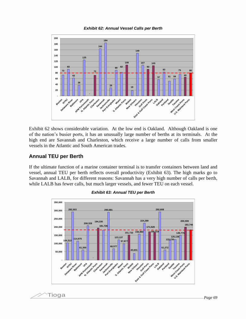
Page 69Tioga
Exhibit 62: Annual Vessel Calls per Berth
93
62
38
125
-
164
184
28
89
108
149
107
93
105
57
83
59
807573
51 65
19
82
72
-
20
40
60
80
100
120
140
160
180
200
Boston
NYNJ
Delawar
e River
Baltim
oreVPA
APMPorts
mouth
N. Atla
nticPorts
Charles
ton
Savan
nah
Jack
sonvil
le
PortEve
rglad
es
Miami
S. Atla
nticPorts
Mobile
NewOrle
ans
Houston
GulfPorts
East &
GulfCoas
t PortsLALB
Oaklan
d
Portlan
d
Seattl
e
Tacom
a
Wes
t Coast Ports
U.S. M
ainlan
dPorts
Exhibit 62 shows considerable variation. At the low end is Oakland. Although Oakland is oneof the nation’s busier ports, it has an unusually large number of berths at its terminals. At thehigh end are Savannah and Charleston, which receive a large number of calls from smallervessels in the Atlantic and South American trades.
Annual TEU per Berth
If the ultimate function of a marine container terminal is to transfer containers between land andvessel, annual TEU per berth reflects overall productivity (Exhibit 63). The high marks go toSavannah and LALB, for different reasons: Savannah has a very high number of calls per berth,while LALB has fewer calls, but much larger vessels, and fewer TEU on each vessel.
Exhibit 63: Annual TEU per Berth
104,313
292,503
114,975
61,300
208,328
-
290,681
68,577
123,137
151,733 156,883
224,289
292,608
61,272
149,775
181,726 171,529
166,518
125,136
183,746
122,730
200,599
40,601
97,877
194,330
-
50,000
100,000
150,000
200,000
250,000
300,000
350,000
Boston
NYNJ
Delawar
e River
Baltim
oreVPA
APMPorts
mouth
N. Atla
nticPorts
Charles
ton
Savan
nah
Jack
sonvil
le
PortEve
rglad
es
Miami
S. Atla
nticPorts
Mobile
NewOrle
ans
Houston
GulfPorts
East &
GulfCoas
t PortsLALB
Oaklan
d
Portlan
d
Seattl
e
Tacom
a
Wes
t Coast Ports
U.S. M
ainlan
dPorts

Page 70Tioga
Berth Call Utilization (Vessel calls per berth vs. maximum calls per berth)
The simplest way to gauge berth capacity utilization is to compare the number of vessels handled(calls) with the maximum that could have been handled (Exhibit 64). The number that couldhave been handled must usually be estimated. The number that could be handled is also affectedby the number of containers discharged and loaded on each one.
Exhibit 64: Berth Call Utilization
43%
30%
18%
60%
0%
71%
13%
43%
52% 51%
27%
40%35%
57%
36%
79%
45%51%
35%39%
25%
31%
9%
40%34%
0%
10%
20%
30%
40%
50%
60%
70%
80%
90%
Boston
NYNJ
Delawar
e River
Baltim
oreVPA
APMPorts
mouth
N. Atla
nticPorts
Charles
ton
Savan
nah
Jack
sonvil
le
PortEve
rglad
es
Miami
S. Atla
nticPorts
Mobile
NewOrle
ans
Houston
GulfPorts
East &
GulfCoas
t PortsLALB
Oaklan
d
Portlan
d
Seattl
e
Tacom
a
Wes
t Coast Ports
U.S. M
ainlan
dPorts
Berth TEU Utilization (Annual TEU per berth vs. maximum TEU per berthfor maximum vessel size)
A more complex look at berth utilization takes into account the maximum TEU that could behandled if the maximum-size vessel made the maximum number of calls (Exhibit 65). This is anaggressive comparison, since it measures productivity against a standard that is unlikely to beattained anywhere. The U.S. average is about 34%. Savannah is at 103%, because the reportedaverage vessel size is larger than the estimated maximum (due to the use of tides for more draft)and the calls per berth measure is high. The West Coast ports have low averages because theircurrent average of vessel size is well below their maximum vessel size.

Page 71Tioga
Exhibit 65: Berth Utilization - Maximum Vessel Size Basis
23%26%
6%
41%
0%
9%
32%
20%
31%
25%19%
25%
10%
89%
39%
21%
42%
10%
72%
0%
10%
20%
30%
40%
50%
60%
70%
80%
90%
100%
Boston
NYNJ
Delawar
e River
Baltim
oreVPA
APMPorts
mouth
Charles
ton
Savan
nah
Jack
sonvil
le
PortEve
rglad
es
Miami
Mobile
NewOrle
ans
Houston
LALB
Oaklan
d
Portlan
d
Seattl
e
Tacom
a
Productivity Implications
Port and terminal throughout could be increased by using larger vessels for the same number ofcalls, making more calls with the same vessels, discharging and loading more of the vesselcapacity at each call, or any combination of these changes. In each case more container cranesand/or crane time would be required to handle the increased cargo while keeping the vessel onschedule. The crane capacity estimates are based on availability for two shifts per day, 250 daysper year (4,000 annual hours). The cranes are, in fact, available 24 hours per day if the terminaloperator needs the additional shifts to turn the vessel on schedule and is willing to pay forovertime.
Berth length and draft determine the size of vessels the terminal can handle and how heavily theycan be loaded. The terminal storage capacity depends on the area available and how high thecontainers can be stacked. The other variable is operating hours. Most terminals will operate asecond shift as required to turn the vessel, but second shifts are expensive, and third shifts arestill more expensive. Most terminals still open the gates for just one shift.
Port authorities are commonly charged by their communities, regions, or states with promotinggrowth of trade, economic development, and jobs. To do so, port and terminal operators attemptto build and maintain sufficient capacity for foreseeable and attainable growth. Most containerterminal parameters that would allow for growth can only be adjusted through large, costly, andtime-consuming long-term commitments. Development of new terminals, expansion of berths,and dredging are multi-year, multi-million dollar projects. Expansion of existing terminal spacecan be undertaken more easily and inexpensively, but can still take months or years in congestedseaport areas.
In the shorter term, ports and terminals can add container cranes at a cost of $5-$10 million each,with a lead time of multiple months rather than multiple years. In the very short term, ports andcontainer terminals can adjust capacity along two dimensions: container yard stacking density
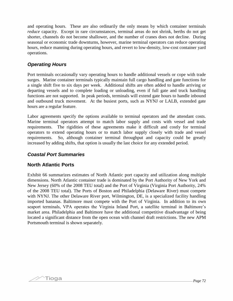
Page 72Tioga
and operating hours. These are also ordinarily the only means by which container terminalsreduce capacity. Except in rare circumstances, terminal areas do not shrink, berths do not getshorter, channels do not become shallower, and the number of cranes does not decline. Duringseasonal or economic trade downturns, however, marine terminal operators can reduce operatinghours, reduce manning during operating hours, and revert to low-density, low-cost container yardoperations.
Operating Hours
Port terminals occasionally vary operating hours to handle additional vessels or cope with tradesurges. Marine container terminals typically maintain full cargo handling and gate functions fora single shift five to six days per week. Additional shifts are often added to handle arriving ordeparting vessels and to complete loading or unloading, even if full gate and truck handlingfunctions are not supported. In peak periods, terminals will extend gate hours to handle inboundand outbound truck movement. At the busiest ports, such as NYNJ or LALB, extended gatehours are a regular feature.
Labor agreements specify the options available to terminal operators and the attendant costs.Marine terminal operators attempt to match labor supply and costs with vessel and traderequirements. The rigidities of these agreements make it difficult and costly for terminaloperators to extend operating hours or to match labor supply closely with trade and vesselrequirements. So, although container terminal throughput and capacity could be greatlyincreased by adding shifts, that option is usually the last choice for any extended period.
Coastal Port Summaries
North Atlantic Ports
Exhibit 66 summarizes estimates of North Atlantic port capacity and utilization along multipledimensions. North Atlantic container trade is dominated by the Port Authority of New York andNew Jersey (60% of the 2008 TEU total) and the Port of Virginia (Virginia Port Authority, 24%of the 2008 TEU total). The Ports of Boston and Philadelphia (Delaware River) must competewith NYNJ. The other Delaware River port, Wilmington, DE, is a specialized facility handlingimported bananas. Baltimore must compete with the Port of Virginia. In addition to its ownseaport terminals, VPA operates the Virginia Inland Port, a satellite terminal in Baltimore’s market area. Philadelphia and Baltimore have the additional competitive disadvantage of beinglocated a significant distance from the open ocean with channel draft restrictions. The new APMPortsmouth terminal is shown separately.
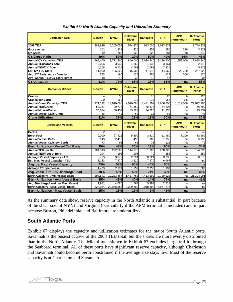
Page 73Tioga
Exhibit 66: North Atlantic Capacity and Utilization Summary
Container Yard Boston NYNJDelaware
RiverBaltimore VPA
APMPortsmouth
N. AtlanticPorts
2008 TEU 208,626 5,265,058 574,876 613,000 2,083,278 8,744,838Gross Acres 101 1,338 420 458 680 230 3,227CY Acres 49 783 120 228 284 78 1,542CY/Gross Ratio 49% 59% 29% 50% 42% 34% 48%Annual CY Capacity - TEU 666,400 8,772,400 840,000 2,634,240 3,126,200 1,659,000 17,698,240Annual TEU/Gross Acre 2,066 3,935 1,369 1,338 3,064 - 2,918Annual TEU/CY Acre 4,258 6,724 4,791 2,689 7,335 - 5,973Est. CY TEU Slots 11,900 125,320 15,000 47,040 44,660 23,700 267,620Avg. CY Slots/ Acre - Density 243 160 125 206 124 306 174Avg. Annual TEU/CY Slot (Turns) 18 42 38 13 47 - 36CY Utilization 31% 75% 68% 23% 83% na 55%
Container Cranes Boston NYNJDelaware
RiverBaltimore VPA
APMPortsmouth
N. AtlanticPorts*
Cranes 4 58 8 16 28 6 120Cranes per Berth 2.0 3.2 1.6 1.6 2.8 1.5 2.4Annual Crane Capacity - TEU 971,192 14,616,000 2,016,000 3,471,202 7,056,000 1,512,000 29,642,395Annual TEU/Crane 52,157 90,777 71,860 38,313 74,403 na 76,709Annual Moves/Crane 30,074 50,432 39,922 24,723 41,335 na 43,137Annual Vessel Calls/Crane 36 42 62 16 63 na 43Crane Utilization 21% 36% 29% 18% 30% na 30%
Berths and Vessels Boston NYNJDelaware
RiverBaltimore VPA
APMPortsmouth
N. AtlanticPorts
Berths 2 18 5 10 10 4 49Berth Feet 2,000 27,421 5,300 8,819 11,460 3,200 58,200Annual Vessel Calls 145 2,419 499 380 1,752 na 5,195Annual Vessel Calls per Berth 73 93 62 38 125 na 72Berth Utilization - Vessel Call Basis 35% 43% 30% 18% 60% na 34%Annual TEU per Berth 104,313 292,503 114,975 61,300 208,328 na 194,330Annual TEU/Foot of Berth 104 192 108 70 182 na 159Average Vessel Capacity - TEU 3,765 3,979 2,234 3,324 3,733 na 3,675Est. Max. Vessel Capacity - TEU 5,183 7,470 3,420 7,470 6,967 na naAvg. vs. Max. Vessel Capacity 73% 53% 65% 44% 54% na naAverage TEU per Vessel 1,439 2,177 1,152 2,358 1,189 na 1,683Avg. Vessel Ute. - % Discharge/Load 38% 55% 52% 71% 32% na 46%Berth Capacity - Avg. Vessel Basis 598,541 12,223,467 1,437,766 4,413,600 2,720,628 na 21,394,001Berth Utilization - Avg. Vessel Basis 35% 43% 40% 14% 77% na 41%Avg. Discharge/Load per Max. Vessel 1,981 4,086 1,764 5,299 2,219 na naBerth Capacity - Max. Vessel Basis 823,934 22,948,363 2,200,890 9,918,893 5,077,716 na naBerth Utilization - Max. Vessel Basis 25% 23% 26% 6% 41% na na
As the summary data show, reserve capacity in the North Atlantic is substantial, in part becauseof the shear size of NYNJ and Virginia (particularly if the APM terminal is included) and in partbecause Boston, Philadelphia, and Baltimore are underutilized.
South Atlantic Ports
Exhibit 67 displays the capacity and utilization estimates for the major South Atlantic ports.Savannah is the busiest at 39% of the 2008 TEU total, but the shares are more evenly distributedthan in the North Atlantic. The Miami total shown in Exhibit 67 excludes barge traffic throughthe Seaboard terminal. All of these ports have significant reserve capacity, although Charlestonand Savannah could become berth-constrained if the average size stays low. Most of the reservecapacity is at Charleston and Savannah.

Page 74Tioga
Exhibit 67: South Atlantic Capacity and Utilization Summary
Container Yard Charleston Savannah JacksonvillePort
EvergladesMiami
S. AtlanticPorts
2008 TEU 1,635,534 2,616,126 754,352 985,095 685,139 6,676,245Gross Acres 1,045 1,200 1,085 315 194 3,839CY Acres 453 495 361 267 139 1,715CY/Gross Ratio 43% 41% 33% 85% 72% 45%Annual CY Capacity - TEU 6,605,760 7,238,560 3,090,080 2,318,400 1,292,480 20,545,280Annual TEU/Gross Acre 1,565 2,180 695 3,127 3,532 1,739Annual TEU/CY Acre 3,610 5,285 2,090 3,689 4,929 3,893Est. CY TEU Slots 117,960 129,260 55,180 41,400 23,080 366,880Avg. CY Slots/ Acre - Density 260 261 153 155 166 214Avg. Annual TEU/CY Slot (Turns) 14 20 14 24 30 18CY Utilization 25% 36% 24% 42% 53% 32%
Container Cranes Charleston Savannah JacksonvillePort
EvergladesMiami
S. AtlanticPorts
Cranes 19 23 18 8 9 77Cranes per Berth 2.1 2.6 1.6 1.0 1.3 1.8Annual Crane Capacity - TEU 4,642,917 5,777,192 4,536,000 2,016,000 2,205,877 19,177,987Annual TEU/Crane 86,081 113,745 41,908 123,137 76,127 86,704Annual Moves/Crane 49,317 63,397 23,282 68,409 43,484 48,739Annual Vessel Calls/Crane 78 79 17 89 64 61Crane Utilization 35% 45% 17% 49% 31% 35%
Berths and Vessels Charleston Savannah JacksonvillePort
EvergladesMiami
S. AtlanticPorts
Berths 9 9 11 8 7 44Berth Feet 7,940 9,693 9,850 6,125 6,500 40,108Annual Vessel Calls 1,475 1,659 307 715 576 4,732Annual Vessel Calls per Berth 164 184 28 89 82 108Berth Utilization - Vessel Call Basis 79% 71% 13% 43% 40% 52%Annual TEU per Berth 181,726 290,681 68,577 123,137 97,877 151,733Annual TEU/Foot of Berth 206 270 77 161 105 166Average Vessel Capacity - TEU 3,695 4,093 2,365 2,289 3,121 3,466Est. Max. Vessel Capacity - TEU 6,031 4,067 3,420 4,067 4,067 naAvg. vs. Max. Vessel Capacity 61% 101% 69% 56% 77% naAverage TEU per Vessel 1,109 1,577 2,457 1,378 2,059 1,411Avg. Vessel Ute. - % Discharge/Load 30% 39% 104% 60% 66% 41%Berth Capacity - Avg. Vessel Basis 1,383,828 2,952,012 5,622,011 1,719,439 2,570,079 14,247,368Berth Utilization - Avg. Vessel Basis 118% 89% 13% 57% 27% 47%Avg. Discharge/Load per Max. Vessel 1,810 1,567 3,553 2,448 2,683 naBerth Capacity - Max. Vessel Basis 2,258,566 2,933,090 8,129,312 3,054,850 3,348,897 naBerth Utilization - Max. Vessel Basis 72% 89% 9% 32% 20% na
Gulf Ports
Exhibit 68 summarizes capacity and utilization estimates for the three major Gulf Coastcontainer ports. Houston dominates the region with 80% of the total, and has most of the reservecapacity. New Orleans suffered a setback from Hurricane Katrina and has a competitivedisadvantage from being located roughly 100 miles upriver from the Gulf of Mexico. Mobile,however, has a new terminal and significant reserve capacity for post-recession growth.
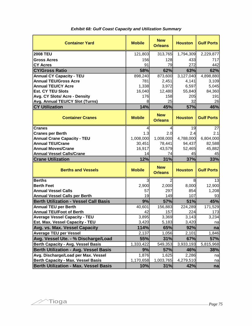
Page 75Tioga
Exhibit 68: Gulf Coast Capacity and Utilization Summary
Container Yard MobileNew
OrleansHouston Gulf Ports
2008 TEU 121,803 313,765 1,794,309 2,229,877Gross Acres 156 128 433 717CY Acres 91 79 272 442CY/Gross Ratio 58% 62% 63% 62%Annual CY Capacity - TEU 898,240 873,600 3,127,040 4,898,880Annual TEU/Gross Acre 781 2,451 4,141 3,109Annual TEU/CY Acre 1,338 3,972 6,597 5,045Est. CY TEU Slots 16,040 12,480 55,840 84,360Avg. CY Slots/ Acre - Density 176 158 205 191Avg. Annual TEU/CY Slot (Turns) 8 25 32 26CY Utilization 14% 45% 57% 46%
Container Cranes MobileNew
OrleansHouston Gulf Ports
Cranes 4 4 19 27Cranes per Berth 1.3 2.0 2.4 2.1Annual Crane Capacity - TEU 1,008,000 1,008,000 4,788,000 6,804,000Annual TEU/Crane 30,451 78,441 94,437 82,588Annual Moves/Crane 16,917 43,579 52,465 45,882Annual Vessel Calls/Crane 14 74 45 45Crane Utilization 12% 31% 37% 33%
Berths and Vessels MobileNew
OrleansHouston Gulf Ports
Berths 3 2 8 13Berth Feet 2,900 2,000 8,000 12,900Annual Vessel Calls 57 297 854 1,208Annual Vessel Calls per Berth 19 149 107 93Berth Utilization - Vessel Call Basis 9% 57% 51% 45%Annual TEU per Berth 40,601 156,883 224,289 171,529Annual TEU/Foot of Berth 42 157 224 173Average Vessel Capacity - TEU 3,895 3,369 3,143 3,234Est. Max. Vessel Capacity - TEU 3,420 5,183 3,420 naAvg. vs. Max. Vessel Capacity 114% 65% 92% naAverage TEU per Vessel 2,137 1,056 2,101 1,846Avg. Vessel Ute. - % Discharge/Load 55% 31% 67% 57%Berth Capacity - Avg. Vessel Basis 1,333,422 549,353 3,933,193 5,815,968Berth Utilization - Avg. Vessel Basis 9% 57% 46% 38%Avg. Discharge/Load per Max. Vessel 1,876 1,625 2,286 naBerth Capacity - Max. Vessel Basis 1,170,658 1,003,765 4,279,510 naBerth Utilization - Max. Vessel Basis 10% 31% 42% na
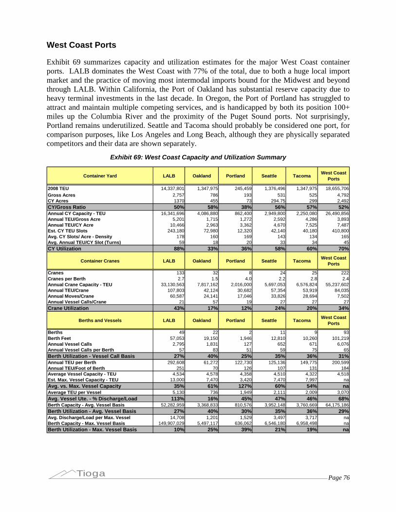
Page 76Tioga
West Coast Ports
Exhibit 69 summarizes capacity and utilization estimates for the major West Coast containerports. LALB dominates the West Coast with 77% of the total, due to both a huge local importmarket and the practice of moving most intermodal imports bound for the Midwest and beyondthrough LALB. Within California, the Port of Oakland has substantial reserve capacity due toheavy terminal investments in the last decade. In Oregon, the Port of Portland has struggled toattract and maintain multiple competing services, and is handicapped by both its position 100+miles up the Columbia River and the proximity of the Puget Sound ports. Not surprisingly,Portland remains underutilized. Seattle and Tacoma should probably be considered one port, forcomparison purposes, like Los Angeles and Long Beach, although they are physically separatedcompetitors and their data are shown separately.
Exhibit 69: West Coast Capacity and Utilization Summary
Container Yard LALB Oakland Portland Seattle TacomaWest Coast
Ports
2008 TEU 14,337,801 1,347,975 245,459 1,376,496 1,347,975 18,655,706Gross Acres 2,757 786 193 531 525 4,792CY Acres 1370 455 73 294.75 299 2,492CY/Gross Ratio 50% 58% 38% 56% 57% 52%Annual CY Capacity - TEU 16,341,696 4,086,880 862,400 2,949,800 2,250,080 26,490,856Annual TEU/Gross Acre 5,201 1,715 1,272 2,592 4,286 3,893Annual TEU/CY Acre 10,466 2,963 3,362 4,670 7,525 7,487Est. CY TEU Slots 243,180 72,980 12,320 42,140 40,180 410,800Avg. CY Slots/ Acre - Density 178 160 169 143 134 165Avg. Annual TEU/CY Slot (Turns) 59 18 20 33 34 45CY Utilization 88% 33% 36% 58% 60% 70%
Container Cranes LALB Oakland Portland Seattle TacomaWest Coast
Ports
Cranes 133 32 8 24 25 222Cranes per Berth 2.7 1.5 4.0 2.2 2.8 2.4Annual Crane Capacity - TEU 33,130,563 7,817,162 2,016,000 5,697,053 6,576,824 55,237,602Annual TEU/Crane 107,803 42,124 30,682 57,354 53,919 84,035Annual Moves/Crane 60,587 24,141 17,046 33,826 28,694 7,502Annual Vessel Calls/Crane 21 57 19 27 27 27Crane Utilization 43% 17% 12% 24% 20% 34%
Berths and Vessels LALB Oakland Portland Seattle TacomaWest Coast
Ports
Berths 49 22 2 11 9 93Berth Feet 57,053 19,150 1,946 12,810 10,260 101,219Annual Vessel Calls 2,795 1,831 127 652 671 6,076Annual Vessel Calls per Berth 57 83 51 59 75 65Berth Utilization - Vessel Call Basis 27% 40% 25% 35% 36% 31%Annual TEU per Berth 292,608 61,272 122,730 125,136 149,775 200,599Annual TEU/Foot of Berth 251 70 126 107 131 184Average Vessel Capacity - TEU 4,534 4,578 4,358 4,510 4,322 4,518Est. Max. Vessel Capacity - TEU 13,000 7,470 3,420 7,470 7,997 naAvg. vs. Max. Vessel Capacity 35% 61% 127% 60% 54% naAverage TEU per Vessel 5,130 736 1,949 2,111 2,009 3,070Avg. Vessel Ute. - % Discharge/Load 113% 16% 45% 47% 46% 68%Berth Capacity - Avg. Vessel Basis 52,282,959 3,368,833 810,576 3,952,148 3,760,669 64,175,186Berth Utilization - Avg. Vessel Basis 27% 40% 30% 35% 36% 29%Avg. Discharge/Load per Max. Vessel 14,708 1,201 1,529 3,497 3,717 naBerth Capacity - Max. Vessel Basis 149,907,029 5,497,117 636,062 6,546,180 6,958,498 naBerth Utilization - Max. Vessel Basis 10% 25% 39% 21% 19% na

Page 77Tioga
Drayage Measures
Turn Time
The most important measure of drayage productivity is “turn time,”the time the motor carrierrequires to conduct a transaction or set of transactions at the marine terminal. The portion of theturn time that is spent inside the marine terminal is regularly measured by the terminal operatorsand is sometimes available. The portion of the turn time that is spent outside the gate is seldommeasured.
Tioga recently conducted a study where both elements were measured. The results are displayedin Exhibit 70, which shows the difference between inside the gate turn times and total turn times.In this case a Qualcomm equipped motor carrier geofenced the marine terminals and was able toprovide total turn time information.
Exhibit 70: Example of Drayage Turn Times
0%
2%
4%
6%
8%
10%
12%
14%
16%
18%
20%
0-15
15-3
030
-45
45-6
060
-75
75-9
0
90-1
05
105-
120
120-
135
135-
150
150-
165
165-
180
180-
195
195-
210
210-
225
225-
240
240-
255
255-
270
270-
285
285-
300
Example Terminal Turn Time
Port-wide Trucker Turn Time
Marine terminals may collect detailed turn time information by type of transaction. This isimportant because all “turns” are not equally difficult. Some visits to a marine terminal may involve a “double move,”that is dropping an export container and picking up an import.Conversely, a transaction may be as simple as delivering an empty container to a marine terminaland bobtailing away. The data in Exhibit 70 do not distinguish between simple and complextransactions.
Another way to analyze turn times is to measure and manage how long each step in the processtakes. The gate process is one example. Exhibit 71 shows a frequency distribution at two marineterminals for which process times were measured using gate cameras. It illustrates that, whilemost gate transactions are handled in under 5 minutes, there are a significant number of longertransactions. The implication is that attacking the exceptionally long transactions will not onlyimprove average turn time, but also make queue time more predictable for motor carriers whosometimes wait in line behind unusually long transactions.

Page 78Tioga
Exhibit 71: Gate Process Time
0%
5%
10%
15%
20%
25%
0-1
2-3
4-5
6-7
8-9
10-1
112
-13
14-1
516
-17
18-1
920
-21
22-2
324
-25
26-2
728
-29
30-3
132
-33
34-3
5
Minutes
Terminal ATerminal B
5% of the moves use 14-18% of the total time and
back up the queue
Trouble Ticket Share
This measure compares the number of transactions involving trouble tickets to the total numberof transactions. A typical trouble ticket share is 5%. Trouble tickets measure the ability of thecustomer, line, terminal, motor carrier, and regulatory agencies to communicate effectively. Thelarge majority of this communication is routine, repetitious, and electronic. For the 5% of thetransactions that the systems mishandle, expensive human intervention is necessary. Eachtrouble ticket typically costs the motor carrier approximately an hour ($50-$60) to resolve.Exhibit 72 is a list of causes for trouble tickets at one terminal Tioga recently studied.
Exhibit 72: Causes of Trouble Tickets
BOOKING PROBLEMS 28%Booking does not match equipment type 10%Booking is not on file 7%Booking tally has already been reached 7%Missing notice for hazardous cargo 3%Booking quantity exceeded for equipment type 3%DISPATCH PROBLEMS 29%Cargo not yet released 8%Driver or motor carrier credential problem 7%Empty Container/chassis not allowed 6%Past cargo cutoff 3%Demurrage due (unpaid bills) 3%Container exceeds maximum safe weight 2%SYSTEM PROBLEMS 22%Container/chassis not recognized 18%Duplicate transaction 2%Container not found in yard 2%Other 20%TOTAL 100%
In the study mentioned above, Tioga observed that inexperienced drivers and motor carriers havemuch higher trouble ticket rates than firms and drivers for whom marine drayage is a primarybusiness.
Page 79Tioga
Best Drayage Practices
The study team attempted to identify best practices to mitigate drayage bottlenecks, delays, andextra trips. There are a number of industry practices and trends that can be expected to improveoverall drayage/marine terminal performance, such as having remote container yards, neutralchassis pools, trucker-supplied chassis, or automated gates. There is a second category ofpractices that focus on information flow, business strategies, and problem solving.
Remote Container Yards. Recently the Uniform Intermodal Interchange Agreement wasmodified to permit marine terminals to direct motor carriers returning empty containers tocontainer yards in the region rather than bringing them back to the marine terminal of origin.
This change was made to accommodate the current empty equipment management practices,which reflect the increasing ability of the lines and terminals to more intensely manage emptyequipment using Internet postings and e-mail to expedite communications with motor carriers.In this case, the practice permits the seamless integration of less expensive container yards inequipment management strategies, particularly for drop off, storage, and pick up of emptyequipment.
This practice has a number of advantages and disadvantages for both motor carrier and terminal:
The marine terminal obtains extra CY and gate capacity, as every movement andfunction handled at the Polaris Street Yard makes additional capacity at PNCT.
The motor carrier seeking to drop off and/or pick up an empty container shouldenjoy a faster gate and overall faster turn times as he is not standing in line behindmore complex transactions.
Conversely, the motor carrier seeking to drop an empty box and pick up a loadhas extra work. The motor carrier does not know exactly what service will berequired when the price is established. As a result, this provision only applies toregional container yards and instructions posted before the close of business theprevious day.
Neutral/Cooperative Chassis Pools. Use of neutral chassis pools is expanding, althoughsuccess has not been uniform. Just as the legacy system of chassis supply is seen as a majorobstacle to drayage and terminal productivity, neutral chassis pools are seen as a near-termsolution and candidates for best practices. Neutral chassis pools appear to have the greatestbenefits at multi-carrier marine terminals and off-dock rail terminals where the need to matchchassis and container ownership leads to delays, exceptions, and large on-site chassis fleets.Neutral chassis pools reduce the total number of chassis required and typically reduce thefrequency of roadability issues. Typically, pools are located at marine terminals, and involveseveral marine and rail facilities in a region.
Customer/Trucker-Supplied Chassis. In the long term, the system would benefit greatly ifocean carriers exited the chassis supply function entirely and chassis were supplied by eitherdrayage firms or customers. Such an industry-wide change would eliminate on-terminal chassis
Page 80Tioga
searches, trouble tickets, and disputes related to chassis conditions, the need to inspect andinterchange chassis at terminal gates, and the need for chassis flips.
Maersk recently took a step in this direction by establishing a practice in which the motor carrierwas made responsible for providing the chassis. It established a chassis leasing company, DirectChassis Link to manage Maersk’s fleet of chassis and provide them to the motor carriers that service Maersk’s (and other) customers. The operating practice now covers most of Maersk’s operations in the United States and is being implemented nationwide. Direct Chassis Linkcharges the motor carrier $11/day for the chassis. When Maersk is responsible for a doordelivery, Maersk pays for the chassis, including any associated customer free time, as part of themotor carrier’s rate.
The practice is designed to reduce the on-terminal chassis storage and chassis managementrequirements in a number of ways:
by providing an incentive for the motor carrier to make double turns with thesame chassis, thereby reducing the number of chassis transactions and increasingutilization,
by providing room in the market for other pool operators to underbid andgradually replace Maersk’s chassis fleet, and
by encouraging the use of motor carrier owned and provided chassis.
Appointment Systems. Appointment systems are largely confined to Southern California atpresent. They have a mixed record there, but hold the potential for wider application to otherports and operators, where they are of interest. Appointment systems have a two-fold purpose:
to allow drayage firms to make efficient dispatching plans with reduced driverqueue times; and
to let marine terminals control workloads, thereby reducing drayage congestionand delay.
Several Southern California appointment systems were tried in response to threats of legislationover driver queue times. Some have fallen into disuse, but the remaining systems have beenimproved and refined. Drayage firms were particularly interested in appointment systems asways of dealing with:
morning queues waiting for gates to open; and
Southern California queues waiting for the 6 PM PierPASS changeover.
Successful appointment systems can be regarded as candidates for best practices. Truckersnoted, however, that appointment systems sometimes do not have enough slots to handle all thecontainers their customers want on the designated day. This observation is symptomatic of theproblems posed by peaking. Motor carriers are also concerned that terminal and customerinefficiencies, as well as variable traffic conditions, may make narrow appointment windowsimpractical, particularly for short- or medium-haul motor carriers that make several trips tomarine terminals daily.
Page 81Tioga
Roadability Canopies. Well-organized, well-supplied, and well-manned “roadability canopies” at or near terminal export gates can quickly remedy minor chassis problems and are regarded ascandidate for best practices. Formerly, it was typical for marine terminals to locate all repairfunctions in a distant corner, forcing drivers to bring problem chassis (or containers) to therepairmen and then back to the exit queue. The practice of locating a “roadability canopy” in line with or in parallel to the exit queue allows drivers to have minor chassis problems remediedwith minimal delay. Well-run roadability operations can deal with typical problems such asbroken light lenses, burnt-out bulbs, missing mud flaps, or low tire pressure in just a fewminutes. The ability to have minor problems corrected quickly reduces the driver’s need to search for a chassis in perfect working order or to incur a large delay for repair. It is also likelythat quick attention to minor problems keeps the chassis fleet in better overall condition thanhaving drivers reject imperfect chassis.
Driver Flexibility/Cutting Losses. Drivers with trouble tickets will typically “cut their losses” after 30 minutes and go on to another transaction rather than wait indefinitely to have a problemresolved. This finding is critical for the correct interpretation of “trouble ticket” data. The timerequired to resolve and close out a trouble ticket is often shared with other driver tasks. Thedriver has not always been fullydelayed. Systems that facilitate the driver’s ability to shift from one problem transaction to other successful ones can be regarded as a candidate for bestpractices. Barriers to switching, such as customer insistence that drivers wait for a problemcontainer or long queues at trouble windows tend to exacerbate delays.
Problem-solving Groups. Regular problem-solving sessions involving marine terminaloperators and drayage firms could make significant progress in dealing with avoidable delaysand trouble tickets. The nature of the working relationship between the parties involveddetermines their ability to exchange information, find common ground, and implement solutions.Facilitating such problem-solving groups could be a useful role for port authorities, who do notdirectly participate in drayage operations but are held publicly responsible for congestion andemissions.
New Driver/Company Orientation. There is a need to help new drivers and firms learn theport, the terminals, and their systems. Some ports, notably Houston and Tacoma, have brochuresaimed at orienting new truck drivers. Useful information would include maps and terminaldiagrams, operating hours, information and documentation requirements, CBP and otherregulations, and key contact information. Most marine terminals provide similar information ontheir websites, but new drivers or firms may not know where to look or what to look for. Theuniversal use of cell phones by drayage drivers may allow the dissemination of such informationvia text messaging or other media.
Effective Two-Stage Gates. The ability to identify exceptions and turnaways early andsegregate them from routine transactions is a key factor in reducing gate congestion and queuetimes. Two-stage gate systems in which the driver, tractor, and transaction are identified andscreened at a first-stage pedestal allow marine terminal operators to turn away unprepareddrivers or direct them to a separate “trouble window”. The gate configuration must have enough distance between first and second stages to take the offending tractor and chassis out of linewithout further disrupting the queue.
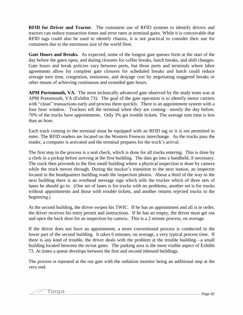
Page 82Tioga
RFID for Driver and Tractor. The consistent use of RFID systems to identify drivers andtractors can reduce transaction times and error rates at terminal gates. While it is conceivable thatRFID tags could also be used to identify chassis, it is not practical to consider their use forcontainers due to the enormous size of the world fleet.
Gate Hours and Breaks. As expected, some of the longest gate queues form at the start of theday before the gates open, and during closures for coffee breaks, lunch breaks, and shift changes.Gate hours and break policies vary between ports, but those ports and terminals where laboragreements allow for complete gate closures for scheduled breaks and lunch could reduceaverage turn time, congestion, emissions, and drayage cost by negotiating staggered breaks orother means of achieving continuous and extended gate hours.
APM Portsmouth, VA. The most technically advanced gate observed by the study team was atAPM Portsmouth, VA (Exhibit 73). The goal of the gate operation is to identify motor carrierswith “clean” transactionsearly and process them quickly. There is an appointment system with afour hour window. Truckers tell the terminal when they are coming—mostly the day before.70% of the trucks have appointments. Only 3% get trouble tickets. The average turn time is lessthan an hour.
Each truck coming to the terminal must be equipped with an RFID tag or it is not permitted toenter. The RFID readers are located on the Western Freeway interchange. As the trucks pass thereader, a computer is activated and the terminal prepares for the truck’s arrival.
The first step in the process is a seal check, which is done for all trucks entering. This is done bya clerk in a pickup before arriving at the first building. The data go into a handheld, if necessary.The truck then proceeds to the first small building where a physical inspection is done by camerawhile the truck moves through. During the trucker’stransition to the next station, an inspectorlocated in the headquarters building reads the inspection photos. About a third of the way to thenext building there is an overhead message sign which tells the trucker which of three sets oflanes he should go to. (One set of lanes is for trucks with no problems, another set is for truckswithout appointments and those with trouble tickets, and another returns rejected trucks to thebeginning.)
At the second building, the driver swipes his TWIC. If he has an appointment and all is in order,the driver receives his entry permit and instructions. If he has an empty, the driver must get outand open the back door for an inspection by camera. This is a 2 minute process, on average.
If the driver does not have an appointment, a more conventional process is conducted in thelower part of the second building. It takes 6 minutes, on average, a very typical process time. Ifthere is any kind of trouble, the driver deals with the problem at the trouble building—a smallbuilding located between the in/out gates. The parking area is the most visible aspect of Exhibit73. At times a queue develops between the first and second inbound buildings.
The process is repeated at the out gate with the radiation monitor being an additional step at thevery end.
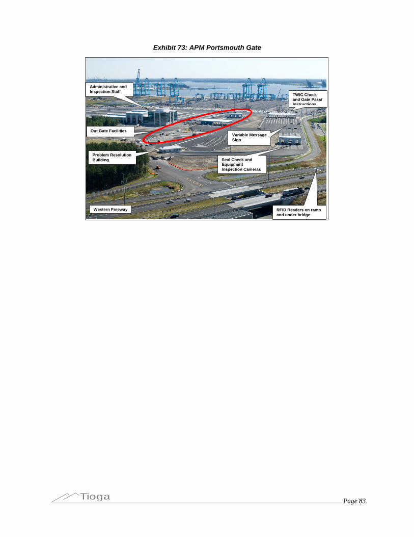
Page 83Tioga
Exhibit 73: APM Portsmouth Gate
Western Freeway RFID Readers on rampand under bridge
Seal Check andEquipmentInspection Cameras
Problem ResolutionBuilding
Out Gate Facilities
Administrative andInspection Staff
TWIC Checkand Gate Pass/Instructions
Variable MessageSign
Page 84Tioga
V. Proposed Data Collection Strategy
Data Requirements
Exhibit 74 summarizes port data items and their uses in port metrics. The entries are color-codedto show relative availability of data.
Exhibit 74: Data for Port Metrics
Available Port Data YieldAlways
Berth Depth Vessels/Gross Acre TEU/Net BGY AcreBerth Length Vessels/CY Acre Gross/Net CY AcresBerths TEU/Gross Acre Net/Gross RatioChannel Depth TEU Slots/CY Acre (Density) CY UtilizationCranes & Types TEU Slots/Gross Acre Moves/ContainerGross Acres TEU/Slot (Turns) DWT/CY AcrePort TEU TEU/CY Acre DWT/Gross AcreVessel Calls Vessels/Net BGY Acre Avg. Dwell TimeVessel DWT
Sometimes Number of Cranes Avg./Max Moves per hourAvg. Crane Moves/hr TEU/Crane TEU/Available Crane HourCY Acres Vessels/Crane TEU/Working Crane HourRail Acres Crane Utilization TEU/Man-HourTEU Slots
Estimated Number of Berths Max Vessel DWT and TEUNet BGY Acres Length of Berths TEU/Vessel TEUVessel TEU Depth of Berth & Channel Vessel TEU/Max Vessel TEUVessel Length TEU/Berth Berth Utilization - TEUAvg. Dwell Time Vessels/Berth Berth Utilization - VesselsBerth Capacity DWT/Berth Vessel Turn TimeCrane CapacityCY Capacity Cranes/Berth Net Acres/Berth
Confidential Gross Acres/Berth Cost/TEUCosts CY Acres/Berth Man-Hours/TEUMan-hours CY Acres/Crane Man-Hours/VesselVessel Turn TimeRatesWorking Crane Hours
Balance & Tradeoffs
Drayage
Land UseAvailable Port Metrics
Crane Use
Berth Use
Data elements and metrics backed in light green are always publicly available (with rareexceptions), and can be used to develop and maintain several of the most useful metrics. Thereare issues of consistency and currency. Different sources can show different figures and it is notalways clear which is more accurate or up to date.
Data elements and metrics backed in yellow are sometimes but not always available from publicsources. Physical measures–CY acres, rail acres, TEU slots–are not particularly confidential inmost cases. The fact that some ports and terminals publish those figures reinforces thatconclusion. Here too there can be issues of consistency and currency.
Data on average moves per crane hour are sometimes published, but may be regarded asconfidential elsewhere and of limited value. As noted in the literature, variations in moves pertotal hour, moves per available hour, moves per shift hour, and moves per working hour all havedifferent implications. There are also questions about the definition of “moves” and treatment of repositioning, re-stowage, and hatch cover handling. Crane productivity measures in moves perhour is a selling point for ports with high-speed cranes or particularly productive labor, and those

Page 85Tioga
ports would be very sensitive to the basis of comparison. The primary audience for craneproductivity data would be the steamship lines. Their ultimate concern, however, is the ability ofthe terminals to turn vessels on time, and crane productivity is only one factor.
Data elements in tan cells in Exhibit 74 were estimated for this study. Some information, such asvessel length and draft data, is potentially available through marine exchanges or other agenciesthat track vessel activity. Considerable work and expense would be required to obtain, analyze,and compile data from roughly twenty marine exchanges. Marine exchanges normally charge fortheir data, either as a one-time report or via subscription.
Average dwell time can be derived from proprietary marine terminal information system data,but would be confidential. Average dwell time, moreover, is of limited applicability to terminalproductivity since the dwell times are a function of customer and carrier interactions. Followingthe 2004 peak season congestion, the Southern California terminal operators reduced thestandard free time allowance in a successful effort to reduce dwell times, especially on imports.Other terminals limit the time an export load can be delivered in advance of vessel arrival toavoid long export dwell times. Empty containers, in contrast, may be stored on-terminal formonths if space is available.
Capacity figures must be estimated and, as noted in the introduction, there are no industry-widestandards or formulas. Different parties will use different assumptions and methodologies toderive different capacity estimates. Ports and terminal operators that do publish capacity figurestypically round them off, sometimes to the nearest million TEU.
Data relating to labor, operating costs, and negotiated rates are confidential and will remain so,as they are proprietary for most businesses.
Note that the data elements described above can be used to develop a number of additionalmetrics besides the core list specified above.
Many data elements are, as noted above, always available. The essential data need is for uniformavailability of “sometimes” data elements via website, association, or directory. Some essentialdata are:
Terminal CY Acres
Terminal rail acres
Terminal TEU slots
Common definitions and conventions would be essential.
Key Barriers to Data Collection
The key data barriers to uniform availability of “sometimes” data elements arise from the natureof the business and its participants.
Page 86Tioga
Marine terminal operators are private, unregulated businesses that consider cost and productivitydata confidential. Ports, which are public entities, do not have access to terminal cost andproductivity data.
There are valid objections to comparisons via many of the possible metrics. Terminals and portsnaturally want to be publicly compared only on metrics where they look good.
Both ports and marine terminal operators compete on cost, and do not want their costs accessibleto either competitors or customers. Negotiated charges to ocean carriers are confidential andsensitive. Labor man-hours and costs are doubly sensitive.
Data Collection and Publication Options
There are two basic ways in which data might be collected, analyzed, and published.
Neutral third party, government agency, or trade association collection andpublishing of confidential data elements
- Ports and/or terminals would provide data to a neutral third party or tradeassociation.
- A third party or association would publish compilations without revealingspecific terminal data.
Confidential benchmarking in exchange for data
- Ports and or terminals would provide data in exchange for a benchmarkingreport comparing their performance with aggregates.
- Only port-wide and aggregate data would be published.
Initial contacts with ports and terminal operators suggest that the second choice is of marginalinterest at present. Because of the data barriers discussed above, and because potential users havenot had experience with benchmarking data, ports and terminal operators do not at present seeenough value to justify internal efforts at comparison. This attitude could change once valid,consistent comparison data become available.
For the present, the first option appears the more viable.
Candidate Organizations
A data collection and publication effort needs a home. The data collection organization needs tobe perceived as objective, needs to have data collection and analysis credibility, and needs tohave subject expertise. The organizations discussed below were considered to be logicalcandidates, although the list may not be exhaustive.
Page 87Tioga
Bureau of Transportation Statistics
The Bureau of Transportation Statistics (BTS) is part of the Research and Innovative TechnologyAdministration (RITA) in the U.S. Department of Transportation. BTS was originallyestablished under ISTEA in 1991, and is currently authorized under SAFETEA-LU (at leastthrough 2009). BTS’s charge is to administer datacollection, analysis, reporting, andpublication across transportation modes. BTS is, in effect, DOT’s central data warehouse. Among its many publications, BTS produces Maritime Trade & Transportation, U.S.International Trade and Freight Transportation Trends, andAmerica’s Container Ports.
BTS also sponsors the Maritime Data Working Group. Its members include:
Bureau of Transportation Statistics
Committee on the Marine Transportation System
Federal Maritime Commission
Maritime Administration
St. Lawrence Seaway Development Corporation
Transportation Security Administration
U.S. Army Corps of Engineers
U.S. Coast Guard
U.S. Department of Agriculture
The Maritime Data Working Group would be a logical sponsor for initiating data collection,computation, and publication within BTS. The group’s mission includes identifying data gaps, making relevant data accessible and promoting standardization and data quality.
BTS would provide the requisite data expertise, stability, objectiveness, and access/publicationcapabilities. BTS maintains a well-organized, regional system for users to locate and orderpublications or data on CD as well as downloading data from www.BTS.gov.
The potential downsides of BTS jurisdiction could include timeliness and industry cooperation.While BTS has annual publications, they are sometimes not updated as quickly as industrysources. Several current BTS publications, for instance, actually contain data only through 2007.Most BTS data compilations are based on information reported through regulatory processes,Customs oversight, etc., as opposed to voluntary compliance.
U.S. Army Corps of Engineers
The U.S. Army Corps of Engineers (USACE) is responsible for development and operations ofthe nation’s waterway system, including seaports. The responsibility includes collecting andmaintaining data. The USACE organization for data collection and publication is the NavigationData Center (NDC) of the Institute for Water Resources, (IWR) in Alexandria, VA. The actual

Page 88Tioga
data collection and database maintenance are done by NDC’s Waterborne Commerce Statistics Center in New Orleans (WCSC).
The strong point of the WCSC program is data on inland waterways and their operations. Themajor WCSC databases include:
Waterborne Commerce of the United States
State Tonnage Reports
Waterborne Transportation Lines of the United States (inland and coastal vesseloperators)
Port Series Reports
The Waterborne Commerce data base is updated annually; the current data are from 2008. ThePort Series Reports, however, are only updated at intervals of up to 10 years. The available datawere reviewed for this study and much of the information was several years old. These reportsmust cover roughly 10,000 U.S. port facilities, and IWR/NDC does not have the resources tocontinually update the data.
IWR has recognized the need for more current data, particularly on container ports whosefacilities often evolve faster, and whose trade base has grown faster than bulk ports andterminals. IWR commissioned the container port capacity analysis that parallels thisproductivity study, and is sharing the port and terminal facility data generated. The Port SeriesReports are compiled from a series of site visits, which is why they are costly and time-consuming to update. It is conceivable that IWR/NDC could update a container port databasecovering about 100 terminals, rather than 10,000, on an annual basis working primarily fromwebsite data, publications, and phone contacts.
Port cooperation may be a potential problem. USACE is responsible for dredging at the ports,and is under continual pressure from those ports. Issues such as draft, vessel size, vesselutilization, etc., can be highly politicized and subject to competing interpretations affectingdredging projects. A port’sproductivity data collection effort could thus be hampered by itsassociation with dredging programs.
If, however, IWR were to choose to update the port capacity database on a regular basis, thedatabase would support many of the recommended productivity metrics.
National Ports and Waterways Institute
The National Ports and Waterways Institute (NPWI) is a research arm of the University of NewOrleans. NPWI’s focus is on research, strategic planning, economics, and regional development. Research and publications tend to be issue-related, as opposed to annual reports. NWPI wastransferred from its original home at Louisiana State University (where it was a cooperativeventure with George Washington University). It retains links to LSU and offices in theWashington, D.C. area.
NWPI researchers may thus be clients or users of port productivity metrics rather than producers.
Page 89Tioga
U.S. Maritime Administration
The U.S. Maritime Administration (MARAD) is the DOT agency dealing with waterbornetransportation. Its vision is to promote development and maintenance of a vital U.S. merchantmarine transportation system. Container ports are part of that broader responsibility. MARADprovides expertise on port financing, infrastructure, and defense deployment readiness.MARAD’s Office of Port Infrastructure Development and Congestion Mitigation (Office) coordinates port studies and surveys. The Office, however, does not have an up-to-date databaseof terminal information and routine data collection is not within theOffice’s charter. The Office is a participant in CHCP, and a major source of motivation and support for this project.
MARAD cooperates with the American Association of Port Authorities (AAPA) to produce twoannual reports (Public Port Finance Survey and U.S. Public Port Development ExpenditureReport) and others as needed. These two reports use industry data collected by AAPA andMARAD’s analytic and publication resources, and present a useful precedent for an annual port productivity report.
American Association of Port Authorities
The American Association of Port Authorities (AAPA) is the industry association for portsthroughout the Americas. About 160 port authorities are members. AAPA is the leading sourcefor container port statistics and offers website access to its databases. Additional data areaccessible through direct contact.
AAPA publishes Seaports of the Americas, a comprehensive directory of ports and terminaloperators produced annually. Seaports of the Americas presents data on ports and terminalssubmitted by port authorities. The data are not consistent in content, format, definition, ortimeliness as AAPA is dependent on its members’ voluntary submissions.
AAPA has four strong recommendations for ongoing development and support of portproductivity metrics.
As the industry’s trade association, AAPA is viewed as a port ally rather than a potential regulator. AAPA may therefore be more likely to gain port cooperation.
AAPA has a regular annual process of consultation with port authorities to obtaininformation for Seaports of the Americas.
AAPA data collection and publication efforts are not subject to Congressionalauthorization or appropriation.
AAPA already collects information and collaborates with MARAD on the twoannual reports described above.
AAPA itself has a relatively small staff and no budget or other resources to collect and compileport productivity data. The Port Finance and Infrastructure Development reports are supportedby MARAD, and a similar arrangement could be developed for a productivity report.
Page 90Tioga
AAPA has on-line profiles of ports in the U.S., Canada, Mexico, Central America, and SouthAmerica. With MARAD support and AAPA member agreement, one publication option wouldbe to add a standardized table or graphic to these on-line profiles.
Initial contact with AAPA suggests that the organization may be amenable to collecting andcompiling container port productivity data with MARAD’s financial or in-kind support.
Recommended Strategy
The most promising strategy for on-going collection, compilation, and publication of containerport productivity data would involve three organizations.
AAPA. The AAPA would collect a standardized set of data elements from itsmembers and publish an annual report. The annual report could be a section ofSeaports of the Americas and/or available on-line.
MARAD. MARAD would provide financial or in-kind support and technicalassistance, and be the U.S. DOT “customer” for productivity data.
USACE IWR/NDC. The U.S. Army Corps of Engineers would share the costwith MARAD and be the federal “customer” for port capacity and infrastructure information supported by the same port data.
This approach would offer the distinct advantage of having the leading industry association andthe two leading federal organizations working from the same data and definitions while sharingthe cost. The resulting data compilations could be made available through AAPA, MARAD,USACE, or BTS as required.
Experience in other data collection efforts suggests that an annual update request may be moreeffective than asking for complete data sets every year. In this approach:
AAPA would either collect the initial data or use the data from this study as astarting point.
Each port authority would designate an AAPA contact.
Each year, the AAPA would send each port a form or electronic file showing themost recent data on record and ask the Port Authority for updates and corrections.Responding to these data-update requests could be combined with existing TEUdata submissions to the AAPA.
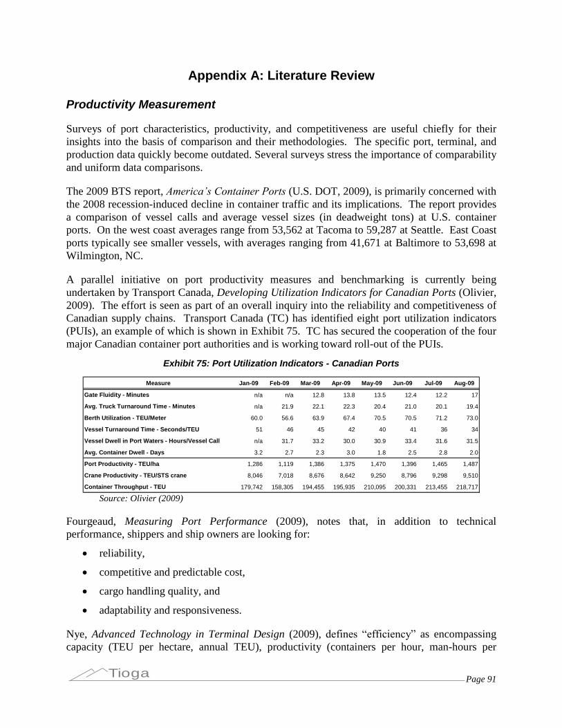
Page 91Tioga
Appendix A: Literature Review
Productivity Measurement
Surveys of port characteristics, productivity, and competitiveness are useful chiefly for theirinsights into the basis of comparison and their methodologies. The specific port, terminal, andproduction data quickly become outdated. Several surveys stress the importance of comparabilityand uniform data comparisons.
The 2009 BTS report,America’s Container Ports(U.S. DOT, 2009), is primarily concerned withthe 2008 recession-induced decline in container traffic and its implications. The report providesa comparison of vessel calls and average vessel sizes (in deadweight tons) at U.S. containerports. On the west coast averages range from 53,562 at Tacoma to 59,287 at Seattle. East Coastports typically see smaller vessels, with averages ranging from 41,671 at Baltimore to 53,698 atWilmington, NC.
A parallel initiative on port productivity measures and benchmarking is currently beingundertaken by Transport Canada, Developing Utilization Indicators for Canadian Ports (Olivier,2009). The effort is seen as part of an overall inquiry into the reliability and competitiveness ofCanadian supply chains. Transport Canada (TC) has identified eight port utilization indicators(PUIs), an example of which is shown in Exhibit 75. TC has secured the cooperation of the fourmajor Canadian container port authorities and is working toward roll-out of the PUIs.
Exhibit 75: Port Utilization Indicators - Canadian Ports
Measure Jan-09 Feb-09 Mar-09 Apr-09 May-09 Jun-09 Jul-09 Aug-09
Gate Fluidity - Minutes n/a n/a 12.8 13.8 13.5 12.4 12.2 17
Avg. Truck Turnaround Time - Minutes n/a 21.9 22.1 22.3 20.4 21.0 20.1 19.4
Berth Utilization - TEU/Meter 60.0 56.6 63.9 67.4 70.5 70.5 71.2 73.0
Vessel Turnaround Time - Seconds/TEU 51 46 45 42 40 41 36 34
Vessel Dwell in Port Waters - Hours/Vessel Call n/a 31.7 33.2 30.0 30.9 33.4 31.6 31.5
Avg. Container Dwell - Days 3.2 2.7 2.3 3.0 1.8 2.5 2.8 2.0
Port Productivity - TEU/ha 1,286 1,119 1,386 1,375 1,470 1,396 1,465 1,487
Crane Productivity - TEU/STS crane 8,046 7,018 8,676 8,642 9,250 8,796 9,298 9,510
Container Throughput - TEU 179,742 158,305 194,455 195,935 210,095 200,331 213,455 218,717
Source: Olivier (2009)
Fourgeaud, Measuring Port Performance (2009), notes that, in addition to technicalperformance, shippers and ship owners are looking for:
reliability,
competitive and predictable cost,
cargo handling quality, and
adaptability and responsiveness.
Nye, Advanced Technology in Terminal Design (2009), defines “efficiency” as encompassingcapacity (TEU per hectare, annual TEU), productivity (containers per hour, man-hours per

Page 92Tioga
move), and terminal cost (land, infrastructure, equipment, systems, and labor). Nye notes thatautomation is not a goal in itself, but a means of striking the best balance between capacity,productivity, and cost (effectively an optimization goal). Nye cites the “end-loaded” terminal design, as implemented at APM Norfolk and proposed for Ports America at Oakland, asparticularly effective at separating vessel and gate traffic and facilitating automation (Exhibit76).
Exhibit 76: End-loaded Container Terminal Design
Source: Nye (2009)
The CT-A terminal at Hamburg is cited as a “state of the art automated terminal” (Exhibit 77).
Exhibit 77: State of the Art Terminal –CT-A Hamburg
Source: Nye (2009)
Nye also provides a case study comparison of cost per vessel lift with various CY technologies(Exhibit 78).
STACK TO GATE/RAILTRANSFER ZONEVESSEL TO STACK
TRANSFER ZONE

Page 93Tioga
Exhibit 78: Terminal Operating Method Comparison
Source: Nye (2009)
Nye concluded that in the case study the top pick/RTG and straddle carrier systems did notprovide sufficient capacity, and that the RTG and side-loaded RMG did not provide adequatevessel productivity due to conflicts with gate traffic. Only the fully-automated, end-loaded RMGoption could meet cost, capacity, and vessel turn-time criteria. Nye’s work also compared dual trolley and tandem lift crane productivity.
Rugaihuruza, Infrastructure, Operational Efficiency and Port Productivity Management inPMAESA Region (2007), asserts that dwell time is the most important factor influencing terminalcapacity. Exhibit 79 shows the relationship for a terminal with a fixed number of storage slots,2,990 in this example.

Page 94Tioga
Exhibit 79: Terminal Capacity versus Container Dwell Time
Source: Rugaihuruza (2007)
Rugaihuruza proposes that port performance be measured in four areas:
Service, where the key factors are vessel turn time and container dwell time
Output, measured by container throughput in TEU
Utilization, including berth occupancy, equipment utilization, and gate utilization
Productivity, in terms of efficiency and cost-effectiveness, measured by (forexample) cost per ton, labor cost per ton, crane moves per hour, containers perman-hour
A white paper prepared for the Maine DOT, Container Terminal Parameters (Cornell Group,Inc. 2007), describes marine container terminal requirements on a conceptual level, alsoproviding a comparison of acres per berth (Exhibit 80). The comparison shows that Californiaterminals average only 40 acres per berth versus higher averages on the other coasts and in thePacific Northwest.
Exhibit 80: Survey of U.S. and Asian Terminals
PORT BERTHS ACRES ACRES/BERTHU.S. North Atlantic 4 178 44.50U.S. Mid-Atlantic 3 219 73.00U.S. South Atlantic 4 193 48.25U.S. Gulf 7 378 54.00U.S. West Coast 80 3200 40.00U.S. PNW #1 2 135 67.50U.S. PNW #2 3 220 73.33East Asian Greenfield 9 640 71.11Median Acres/Berth 60.75
Source: Cornell Group, Inc. (2007)
Beŝkovnik, Measuring and Increasing the Productivity Model on Maritime Container Terminals(2008), defines efficiency in terms of velocity, “a quick transshipment of containers to and from
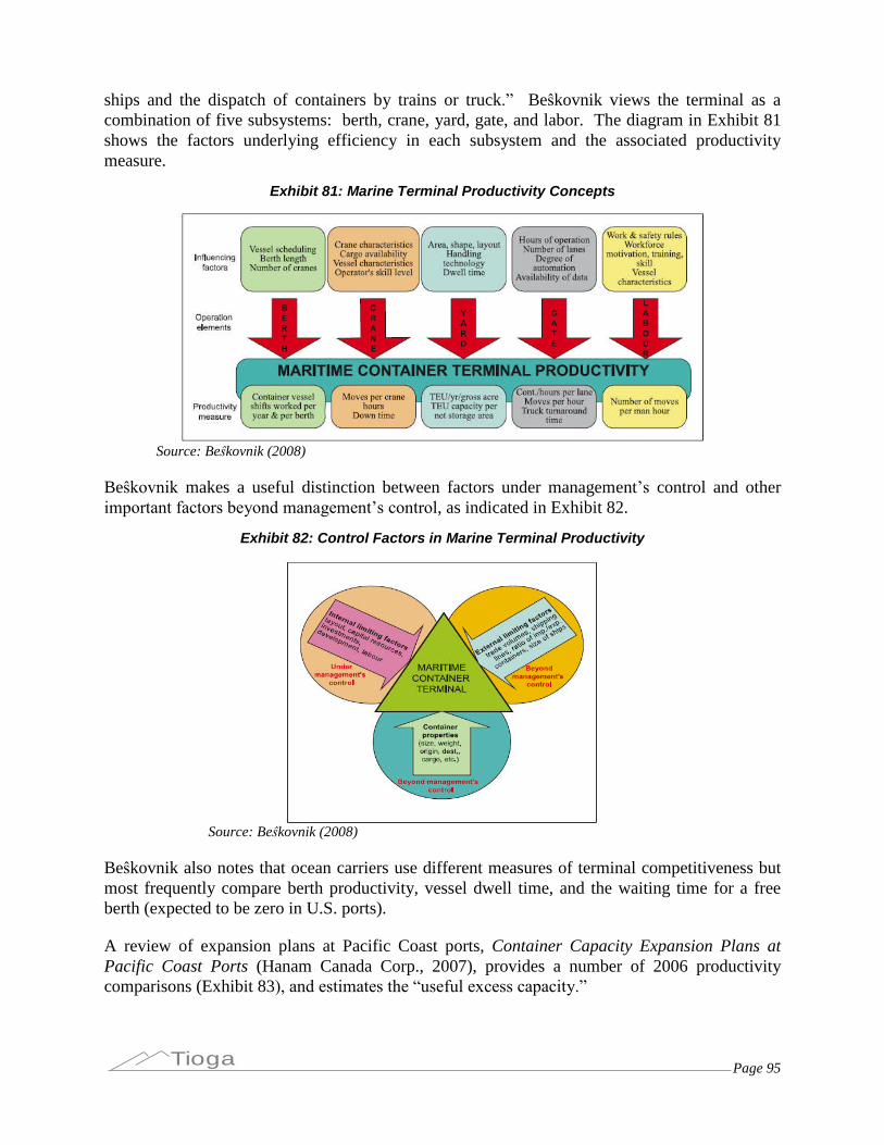
Page 95Tioga
ships and the dispatch of containers by trains or truck.” Beŝkovnik views the terminal as acombination of five subsystems: berth, crane, yard, gate, and labor. The diagram in Exhibit 81shows the factors underlying efficiency in each subsystem and the associated productivitymeasure.
Exhibit 81: Marine Terminal Productivity Concepts
Source: Beŝkovnik (2008)
Beŝkovnik makes a useful distinction between factors under management’scontrol and otherimportant factors beyond management’s control, as indicated in Exhibit 82.
Exhibit 82: Control Factors in Marine Terminal Productivity
Source: Beŝkovnik (2008)
Beŝkovnik also notes that ocean carriers use different measures of terminal competitiveness butmost frequently compare berth productivity, vessel dwell time, and the waiting time for a freeberth (expected to be zero in U.S. ports).
A review of expansion plans at Pacific Coast ports, Container Capacity Expansion Plans atPacific Coast Ports (Hanam Canada Corp., 2007), provides a number of 2006 productivitycomparisons (Exhibit 83), and estimates the “useful excess capacity.”
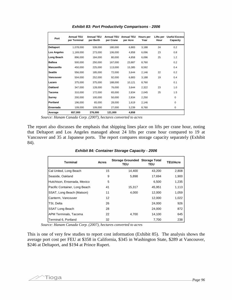
Page 96Tioga
Exhibit 83: Port Productivity Comparisons - 2006
PortAnnual TEUper Terminal
Annual TEUper Berth
Annual TEUper Crane
Annual TEUper Acre
Hours perYear
Lifts perHour
Useful ExcessCapacity
Deltaport 1,078,000 539,000 180,000 6,883 3,188 24 0.2
Los Angeles 1,169,000 273,000 106,000 4,858 6,096 23 0.8
Long Beach 896,000 184,000 80,000 4,858 6,096 25 1.2
Balboa 500,000 250,000 167,000 23,887 8,760 0.2
Manzanillo 450,000 225,000 113,000 15,385 8,592 0.4
Seattle 556,000 185,000 72,000 3,644 2,146 22 0.2
Vancouver 504,000 252,000 92,000 6,883 3,188 19 0.4
Lazaro 375,000 375,000 188,000 10,121 8,760 0.1
Oakland 347,000 128,000 76,000 3,644 2,322 23 1.0
Tacoma 310,000 172,000 65,000 2,834 2,045 25 1.5
Surrey 200,000 100,000 50,000 2,834 2,250 0
Portland 196,000 65,000 28,000 1,619 2,146 0
Ensenada 109,000 109,000 27,000 3,239 8,760 0
Average 657,000 276,000 121,000 4,858
Source: Hanam Canada Corp. (2007), hectares converted to acres
The report also discusses the emphasis that shipping lines place on lifts per crane hour, notingthat Deltaport and Los Angeles managed about 24 lifts per crane hour compared to 19 atVancouver and 35 at Japanese ports. The report compares storage capacity separately (Exhibit84).
Exhibit 84: Container Storage Capacity - 2006
Terminal AcresStorage Grounded
TEUStorage Total
TEUTEU/Acre
Cal United, Long Beach 15 14,400 43,200 2,808
Seaside, Oakland 9 5,898 17,694 1,900
Hutchison, Ensenada, Mexico 5 6,500 1,235
Pacific Container, Long Beach 41 15,317 45,951 1,113
SSAT, Long Beach (Matson) 11 4,000 12,000 1,059
Canterm, Vancouver 12 12,000 1,022
TSI, Delta 26 24,000 926
SSAT Long Beach 28 24,000 872
APM Terminals, Tacoma 22 4,700 14,100 645
Terminal 6, Portland 32 7,700 238
Source: Hanam Canada Corp. (2007), hectares converted to acres
This is one of very few studies to report cost information (Exhibit 85). The analysis shows theaverage port cost per FEU at $358 in California, $345 in Washington State, $289 at Vancouver,$246 at Deltaport, and $194 at Prince Rupert.
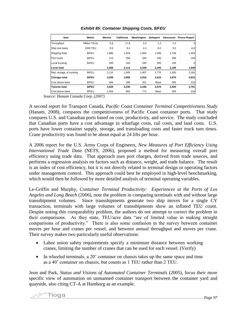
Page 97Tioga
Exhibit 85: Container Shipping Costs, $/FEU
Item Metric Mexico California Washington Deltaport Vancouver Prince Rupert
Throughput Million TEU/y 0.8 17.8 3.3 1.2 1.0 0
Ship size basis 1000 TEU 5.5 9.4 4.4 6.0 3.5 6.0
Shipping Rate $/FEU 1,986 1,593 1,663 1,599 1,746 1,455
Port Costs $/FEU 113 358 345 246 289 194
Local trucking $/FEU 189 163 200 200 150 0
Local total 2,288 2,114 2,208 2,045 2,185 1,649
Rail, storage, & trucking $/FEU 2,110 1,945 1,907 1,770 1,935 2,181
Chicago total $/FEU 4,209 3,895 3,916 3,615 3,970 3,831
Cost above base $/FEU 594 280 301 Base 355 216
Totonto total $/FEU 4,639 4,230 4,346 3,575 3,930 3,791
Cost above base $/FEU 1,064 655 771 Base 355 216
Source: Hanam Canada Corp. (2007)
A second report for Transport Canada, Pacific Coast Container Terminal Competitiveness Study(Hanam, 2008), compares the competitiveness of Pacific Coast container ports. That studycompares U.S. and Canadian ports based on cost, productivity, and service. The study concludedthat Canadian ports have a cost advantage in wharfage costs, rail costs, and land costs. U.S.ports have lower container supply, storage, and transloading costs and faster truck turn times.Crane productivity was found to be about equal at 24 lifts per hour.
A 2006 report for the U.S. Army Corps of Engineers, New Measures of Port Efficiency UsingInternational Trade Data (NETS, 2006), proposed a method for measuring overall portefficiency using trade data. That approach uses port charges, derived from trade sources, andperforms a regression analysis on factors such as distance, weight, and trade balance. The resultis an index of cost efficiency, but it is not directly related to terminal design or operating factorsunder management control. This approach could best be employed in high-level benchmarking,which would then be followed by more detailed analysis of terminal operating variables.
Le-Griffin and Murphy, Container Terminal Productivity: Experiences at the Ports of LosAngeles and Long Beach (2006), note the problem in comparing terminals with and without largetransshipment volumes. Since transshipments generate two ship moves for a single CYtransaction, terminals with large volumes of transshipments show an inflated TEU count.Despite noting this comparability problem, the authors do not attempt to correct the problem intheir comparisons. As they state, TEU/acre data “are of limited value in making straight comparisons of productivity.” There is also some confusion in the survey between containermoves per hour and cranes per vessel, and between annual throughput and moves per crane.Their survey makes two particularly useful observations:
Labor union safety requirements specify a minimum distance between workingcranes, limiting the number of cranes that can be used for each vessel. (Verify)
In wheeled terminals, a 20’ container on chassis takes up the same space and time as a 40’ container on chassis, but counts as 1 TEU rather than 2 TEU.
Jeon and Park, Status and Visions of Automated Container Terminals (2005), focus their morespecific view of automation on unmanned container transport between the container yard andquayside, also citing CT-A at Hamburg as an example.
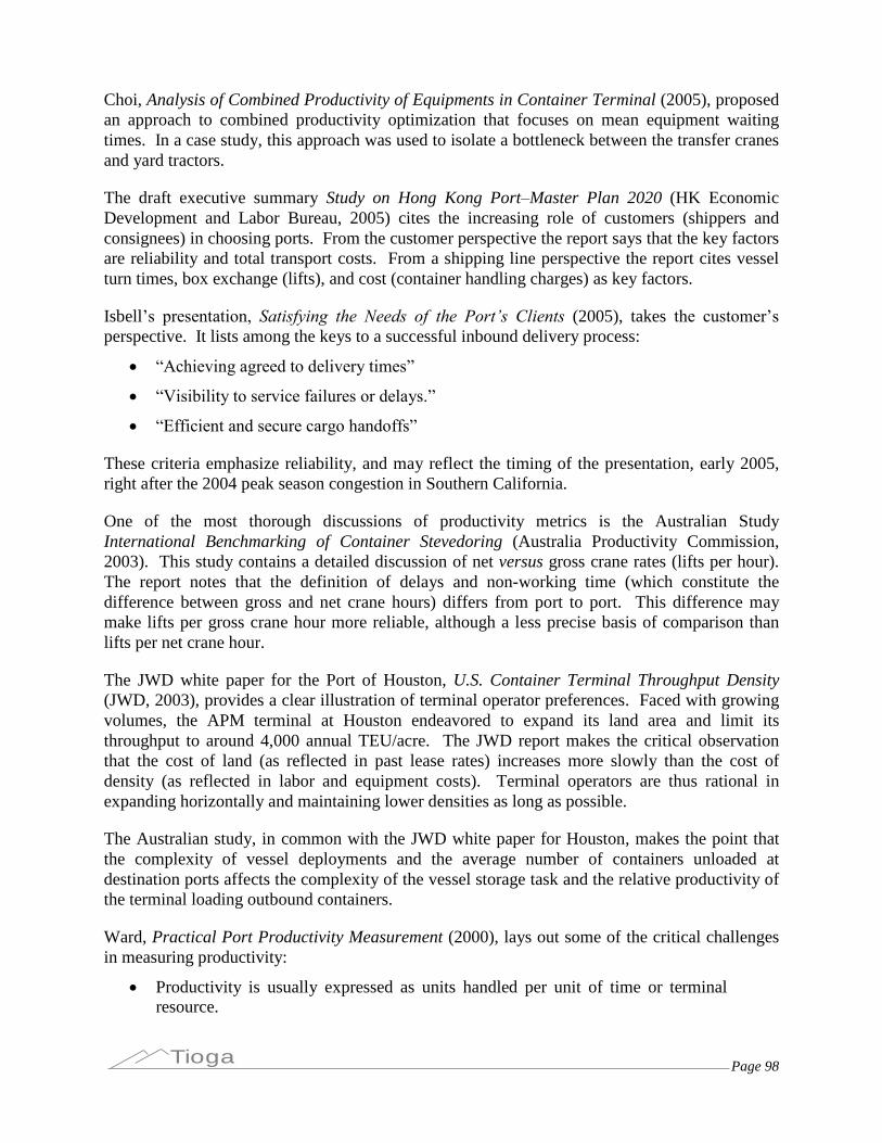
Page 98Tioga
Choi, Analysis of Combined Productivity of Equipments in Container Terminal (2005), proposedan approach to combined productivity optimization that focuses on mean equipment waitingtimes. In a case study, this approach was used to isolate a bottleneck between the transfer cranesand yard tractors.
The draft executive summary Study on Hong Kong Port–Master Plan 2020 (HK EconomicDevelopment and Labor Bureau, 2005) cites the increasing role of customers (shippers andconsignees) in choosing ports. From the customer perspective the report says that the key factorsare reliability and total transport costs. From a shipping line perspective the report cites vesselturn times, box exchange (lifts), and cost (container handling charges) as key factors.
Isbell’s presentation, Satisfying the Needs of the Port’s Clients(2005), takes the customer’s perspective. It lists among the keys to a successful inbound delivery process:
“Achieving agreed to delivery times”
“Visibility to service failures or delays.”
“Efficient and secure cargo handoffs”
These criteria emphasize reliability, and may reflect the timing of the presentation, early 2005,right after the 2004 peak season congestion in Southern California.
One of the most thorough discussions of productivity metrics is the Australian StudyInternational Benchmarking of Container Stevedoring (Australia Productivity Commission,2003). This study contains a detailed discussion of net versus gross crane rates (lifts per hour).The report notes that the definition of delays and non-working time (which constitute thedifference between gross and net crane hours) differs from port to port. This difference maymake lifts per gross crane hour more reliable, although a less precise basis of comparison thanlifts per net crane hour.
The JWD white paper for the Port of Houston, U.S. Container Terminal Throughput Density(JWD, 2003), provides a clear illustration of terminal operator preferences. Faced with growingvolumes, the APM terminal at Houston endeavored to expand its land area and limit itsthroughput to around 4,000 annual TEU/acre. The JWD report makes the critical observationthat the cost of land (as reflected in past lease rates) increases more slowly than the cost ofdensity (as reflected in labor and equipment costs). Terminal operators are thus rational inexpanding horizontally and maintaining lower densities as long as possible.
The Australian study, in common with the JWD white paper for Houston, makes the point thatthe complexity of vessel deployments and the average number of containers unloaded atdestination ports affects the complexity of the vessel storage task and the relative productivity ofthe terminal loading outbound containers.
Ward, Practical Port Productivity Measurement (2000), lays out some of the critical challengesin measuring productivity:
Productivity is usually expressed as units handled per unit of time or terminalresource.

Page 99Tioga
Measurement units are not rigorously or consistently defined.
Performance metrics do not match business needs.
Different parties have different needs.
As an example, Ward notes that handling a given vessel could require 24 ship hours, 21 berthhours, 28 gang hours, or 19.5 crane hours. Depending on how over stowed and transshippedboxes are counted, the same vessel call can generate four different lift counts. The lift per hourmetric for the same vessel call could vary from 14.3 to 23.9, depending on definitions andperspective. Ward goes on to carefully define a series of variables and inputs to productivitymetrics.
Vandeveer, Port Productivity Standards for Long-term Planning (1998), in an oft-cited earlypaper, lists four basic measurement concepts:
Throughput per terminal area
Key equipment utilization rates
Berth utilization
Vessel loading/unloading rates
Vandeveer argues that throughput per terminal area provides “order of magnitude benchmarks” and is the most appropriate for land-use planning.
Ashar, Port Productivity Revisited (1997), makes a case for “all-in” port cost per move as a more relevant measure than moves per hour when it comes to competition between ports. Asharsuggests a “productivity-adjusted” price as a more meaningful market pricing system. The ideais that a cost per hour should be limited to moves per hour to account for the non-cash cost ofvessel time.
In an earlier paper, Productivity and Capacity of Container Terminals (1985), Ashar observedthat the new terminals being built at the time were larger versions of older terminals withoutinnovations designed to increase productivity. This is a critical point: terminals are built outrather than up to keep costs low as long as land is readily available. Ashar proposed a terminalarea survey to establish land use within the terminal and a terminal productivity profile using thefollowing indicators:
TEU per gross terminal acre
TEU per CY acre
vessel shifts per berth
moves per crane
moves per crane-hour
These five measures illustrate an important distinction between the productivity of resourceswhen employed (e.g., container moves per crane hour) and the overall utilization of terminal

Page 100Tioga
resources (e.g., annual container moves per crane). This is essentially the task being undertakenin the present study, 25 years later.
Chung, Port Performance Indicators (1993), provides a discussion of port indicators applicableto other types of ports, as well as container ports. Those applicable to container ports include:
Average vessel turn time
TEU per crane hour
Cargo dwell time
Berth occupancy rate (%)
De Monie, Measuring and Evaluating Port Performance and Productivity (1987), argues thatport productivity should be measured with respect to:
duration of a ship’s stay in port
quality of cargo-handling
quality of service to inland transport vehicles.
De Monie breaks down vessel time in port into several components, of which total time at berthand operational (working) time at berth are the most relevant for terminal productivity.
The National Research Council report Improving Productivity in U.S. Marine ContainerTerminals (Committee on Productivity of Marine Terminals, 1986) cites a perceived productivityshortfall at U.S. terminals when compared to foreign terminals. Several contributing factors are:
labor-management relations
improved information systems
automated container identification
At the time of the report (1986) about 46% of the terminals used a grounded system and 54%used a stacking system. The report found “no clear indication” of which was the most productive but noted the superiority of the chassis system in terms of customer service andsatisfaction. The report found that the choice of system was influenced by the availability ofland. The chief basis of comparison between U.S. and foreign terminals was not throughput peracre but utilization–throughput as a percentage of capacity. The report concluded that thereserve capacity of U.S. terminals obviated the need for expansion in most cases. The report alsofound low relative utilization of crane lift capacity (e.g., 20 lifts per hour versus 30-35 lifts perhour in Asia or Europe). The report, most significantly, provided a profile of terminalproductivity measures (Exhibit 86), and made a strong case for standardizing, collecting, andpublishing such measures as a management tool and a spur to improved productivity.

Page 101Tioga
Exhibit 86: Terminal Productivity Measures
Element ofTerminal
Crane Net crane productivity: moves/(gross gang hours - downtime)Gross crane productivity: moves/(gross gang hours)
Berth Net berth utilization: annual container vessel shifts/container berths
Yard Yard throughput: annual TEU/gross acresYard storage productivity: TEU capacity/net storage acre
Gate Net gate throughput: containers per hour/lanesGross gate throughput: equipment moves per hour/lanesTruck turnaround time: total truck time in terminal/number of trucks
Gang Gross labor productivity: number of moves/man-hours
Measure of Productivity
Source: Committee on Productivity of Marine Terminals (1986)
An early Australian survey of port productivity over time, Container Terminal Productivity inPort Jackson from 1977 to 1981 (Bureau of Transport Economics, 1984), emphasized vesseltime in port, noting that differences in vessel sizes and types affected terminal performance. Thestudy compared two terminals at Port Jackson, and took the unusual step of breaking downvessel time into time waiting to berth, time at berth, time working the vessel, and time lost todelays for various reasons. Notably, vessel time at berth was longer at the terminal servinglarger vessels because handling rates were about the same. Although the study itself is dated, theconceptual division of vessel time into functional components is still valuable and applicable.
Capacity and Throughput Studies
Among the most useful sources in the literature are those that analyze the underlying factors incontainer terminal capacity and throughput.
Parsons Brinkerhoff, Strategic Advisory Report: Napoleon Avenue Container TerminalDevelopment Utilizing Public-Private Partnerships (2009), estimated the capacity of a proposednew terminal at the Port of New Orleans on three levels:
Ultimate Theoretical Capacity (UTC). Considered to be the highest theoreticallevel of a terminal’s ability to handle cargo demand. This ultimate capacity value is only constrained by the terminal infrastructure. UTC is not used for facilitysizing, needs identification, or future planning.
Maximum Practical Capacity (MPC). The practical upper limit of a terminal’s ability to handle cargo demand is referred to as MPC. This capacity level isconstrained by infrastructure, equipment, and/or operating capabilities.
Sustainable Practical Capacity (SPC). The SPC is the capacity at whichimprovements should be considered, and generally ranges between 70% and 90%of MPC. For planning purposes, in this analysis, SPC was estimated at 80% ofMPC.
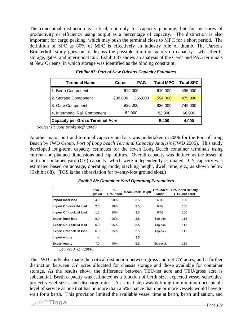
Page 102Tioga
The conceptual distinction is critical, not only for capacity planning, but for measures ofproductivity or efficiency using output as a percentage of capacity. The distinction is alsoimportant for cargo peaking, which may push the terminal close to MPC for a short period. Thedefinition of SPC as 80% of MPC is effectively an industry rule of thumb. The ParsonsBrinkerhoff study goes on to discuss the possible limiting factors on capacity: wharf/berth,storage, gates, and intermodal rail. Exhibit 87 shows an analysis of the Ceres and PAG terminalsat New Orleans, in which storage was identified as the binding constraint.
Exhibit 87: Port of New Orleans Capacity Estimates
Terminal Name Ceres PAG Total MPC Total SPC
1. Berth Component 619,000 495,000
2. Storage Component 238,000 356,000 594,000 475,000
3. Gate Component 936,000 749,000
4. Intermodal Rail Component 82,000 66,000
5,400 4,000
619,000
936,000
82,000
Capacity per Gross Terminal Acre
Source: Parsons Brinkerhoff (2009)
Another major port and terminal capacity analysis was undertaken in 2006 for the Port of LongBeach by JWD Group, Port of Long beach Terminal Capacity Analysis (JWD 2006). This studydeveloped long-term capacity estimates for the seven Long Beach container terminals usingcurrent and planned dimensions and capabilities. Overall capacity was defined as the lesser ofberth or container yard (CY) capacity, which were independently estimated. CY capacity wasestimated based on acreage, operating mode, stacking height, dwell time, etc., as shown below(Exhibit 88). (TGS is the abbreviation for twenty-foot ground slots.)
Exhibit 88: Container Yard Operating Parameters
Dwell(days)
%Grounded
Mean Stack HeightGrounded
ModeGrounded Density
(TGS/net acre)
Import local load 4.0 90% 3.5 RTG 100
Import On-dock IM load 2.0 90% 3.5 RTG 100
Import Off-dock IM load 1.5 90% 3.5 RTG 100
Export local load 6.0 95% 3.5 Top-pick 115
Export On-dock IM load 6.0 95% 3.5 Top-pick 115
Export Off-dock IM load 6.0 95% 3.5 Top-pick 115
Import empty na 3.5
Export empty 7.0 95% 5.5 Side-pick 115
Source: JWD (2006)
The JWD study also made the critical distinction between gross and net CY acres, and a furtherdistinction between CY acres allocated for chassis storage and those available for containerstorage. As the results show, the difference between TEU/net acre and TEU/gross acre issubstantial. Berth capacity was estimated as a function of berth size, expected vessel schedules,project vessel sizes, and discharge rates. A critical step was defining the minimum acceptablelevel of service as one that has no more than a 5% chance that one or more vessels would have towait for a berth. This provision limited the available vessel time at berth, berth utilization, and
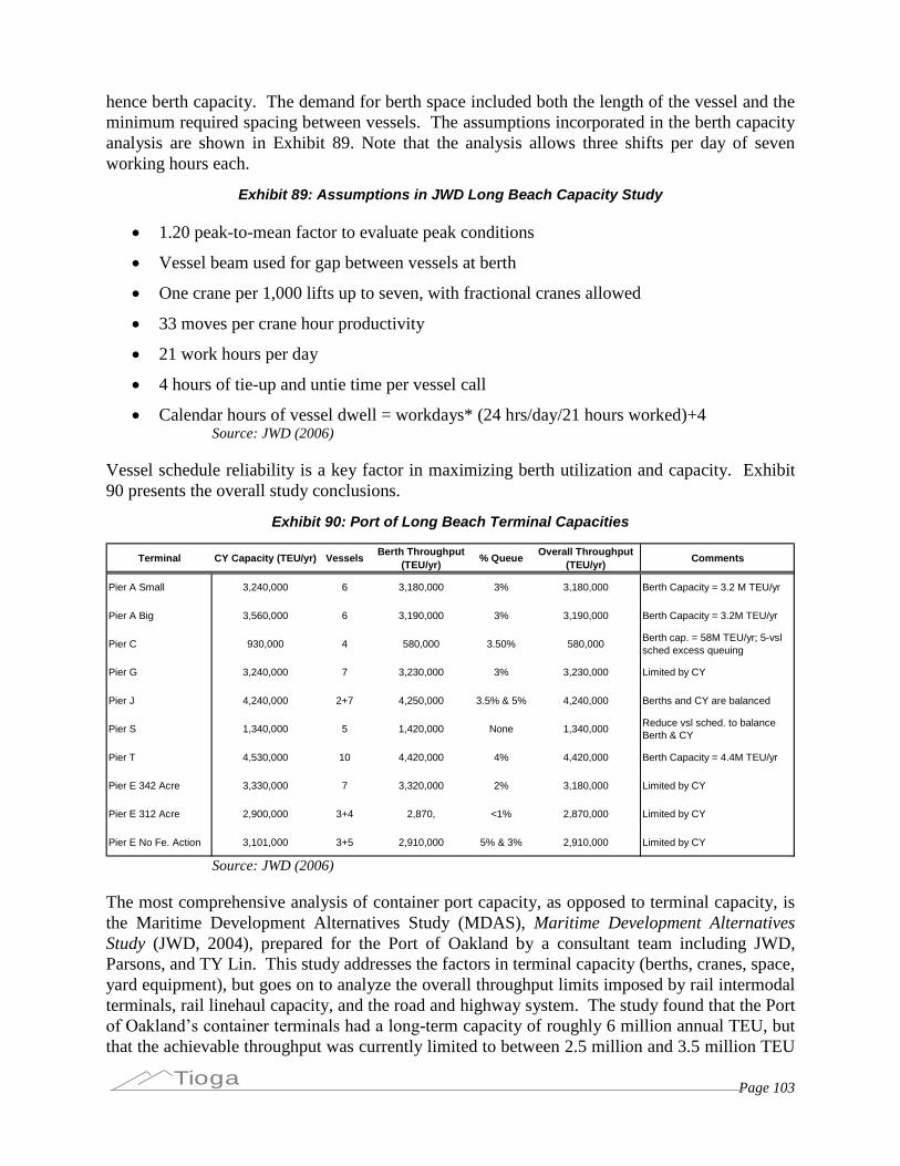
Page 103Tioga
hence berth capacity. The demand for berth space included both the length of the vessel and theminimum required spacing between vessels. The assumptions incorporated in the berth capacityanalysis are shown in Exhibit 89. Note that the analysis allows three shifts per day of sevenworking hours each.
Exhibit 89: Assumptions in JWD Long Beach Capacity Study
1.20 peak-to-mean factor to evaluate peak conditions
Vessel beam used for gap between vessels at berth
One crane per 1,000 lifts up to seven, with fractional cranes allowed
33 moves per crane hour productivity
21 work hours per day
4 hours of tie-up and untie time per vessel call
Calendar hours of vessel dwell = workdays* (24 hrs/day/21 hours worked)+4Source: JWD (2006)
Vessel schedule reliability is a key factor in maximizing berth utilization and capacity. Exhibit90 presents the overall study conclusions.
Exhibit 90: Port of Long Beach Terminal Capacities
Terminal CY Capacity (TEU/yr) VesselsBerth Throughput
(TEU/yr)% Queue
Overall Throughput(TEU/yr)
Comments
Pier A Small 3,240,000 6 3,180,000 3% 3,180,000 Berth Capacity = 3.2 M TEU/yr
Pier A Big 3,560,000 6 3,190,000 3% 3,190,000 Berth Capacity = 3.2M TEU/yr
Pier C 930,000 4 580,000 3.50% 580,000Berth cap. = 58M TEU/yr; 5-vslsched excess queuing
Pier G 3,240,000 7 3,230,000 3% 3,230,000 Limited by CY
Pier J 4,240,000 2+7 4,250,000 3.5% & 5% 4,240,000 Berths and CY are balanced
Pier S 1,340,000 5 1,420,000 None 1,340,000 Reduce vsl sched. to balanceBerth & CY
Pier T 4,530,000 10 4,420,000 4% 4,420,000 Berth Capacity = 4.4M TEU/yr
Pier E 342 Acre 3,330,000 7 3,320,000 2% 3,180,000 Limited by CY
Pier E 312 Acre 2,900,000 3+4 2,870, <1% 2,870,000 Limited by CY
Pier E No Fe. Action 3,101,000 3+5 2,910,000 5% & 3% 2,910,000 Limited by CY
Source: JWD (2006)
The most comprehensive analysis of container port capacity, as opposed to terminal capacity, isthe Maritime Development Alternatives Study (MDAS), Maritime Development AlternativesStudy (JWD, 2004), prepared for the Port of Oakland by a consultant team including JWD,Parsons, and TY Lin. This study addresses the factors in terminal capacity (berths, cranes, space,yard equipment), but goes on to analyze the overall throughput limits imposed by rail intermodalterminals, rail linehaul capacity, and the road and highway system. The study found that the Portof Oakland’s container terminals had a long-term capacity of roughly 6 million annual TEU, butthat the achievable throughput was currently limited to between 2.5 million and 3.5 million TEU
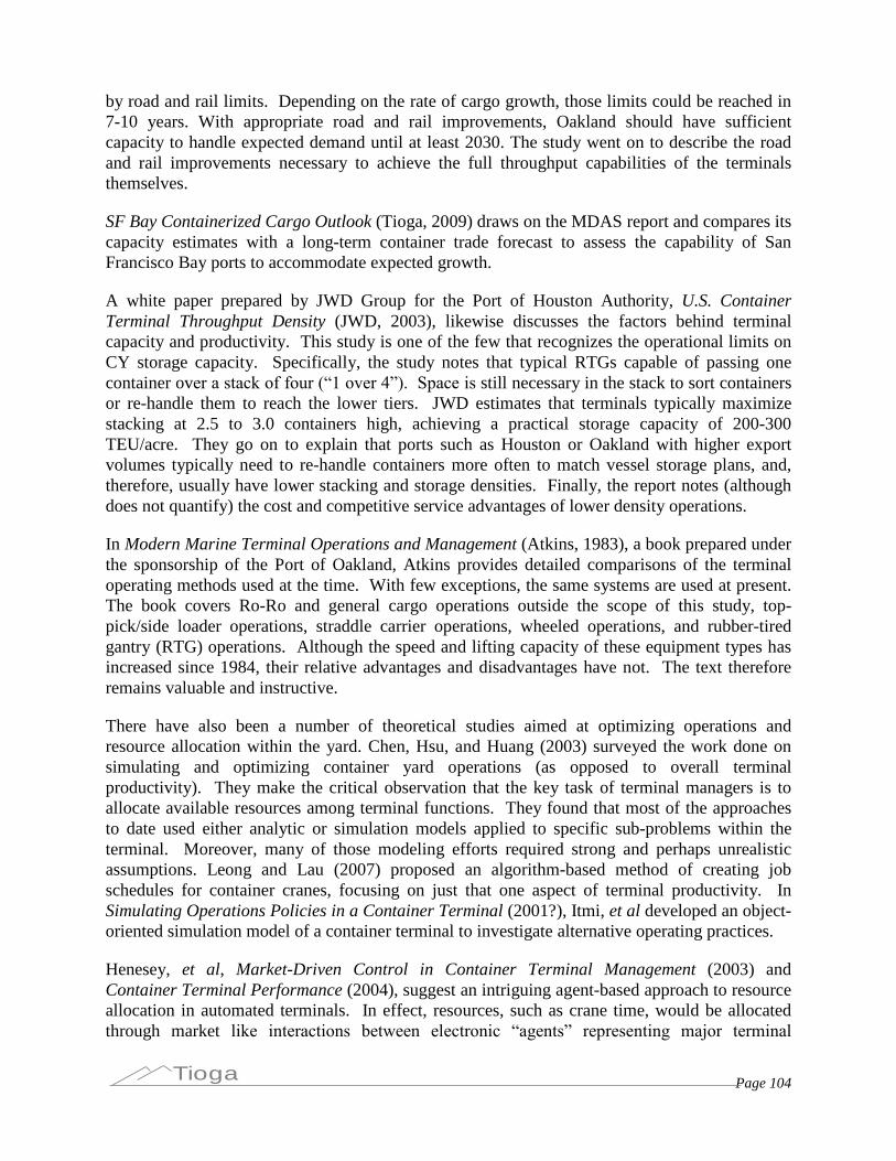
Page 104Tioga
by road and rail limits. Depending on the rate of cargo growth, those limits could be reached in7-10 years. With appropriate road and rail improvements, Oakland should have sufficientcapacity to handle expected demand until at least 2030. The study went on to describe the roadand rail improvements necessary to achieve the full throughput capabilities of the terminalsthemselves.
SF Bay Containerized Cargo Outlook (Tioga, 2009) draws on the MDAS report and compares itscapacity estimates with a long-term container trade forecast to assess the capability of SanFrancisco Bay ports to accommodate expected growth.
A white paper prepared by JWD Group for the Port of Houston Authority, U.S. ContainerTerminal Throughput Density (JWD, 2003), likewise discusses the factors behind terminalcapacity and productivity. This study is one of the few that recognizes the operational limits onCY storage capacity. Specifically, the study notes that typical RTGs capable of passing onecontainer over a stack of four (“1 over 4”). Space is still necessary in the stack to sort containersor re-handle them to reach the lower tiers. JWD estimates that terminals typically maximizestacking at 2.5 to 3.0 containers high, achieving a practical storage capacity of 200-300TEU/acre. They go on to explain that ports such as Houston or Oakland with higher exportvolumes typically need to re-handle containers more often to match vessel storage plans, and,therefore, usually have lower stacking and storage densities. Finally, the report notes (althoughdoes not quantify) the cost and competitive service advantages of lower density operations.
In Modern Marine Terminal Operations and Management (Atkins, 1983), a book prepared underthe sponsorship of the Port of Oakland, Atkins provides detailed comparisons of the terminaloperating methods used at the time. With few exceptions, the same systems are used at present.The book covers Ro-Ro and general cargo operations outside the scope of this study, top-pick/side loader operations, straddle carrier operations, wheeled operations, and rubber-tiredgantry (RTG) operations. Although the speed and lifting capacity of these equipment types hasincreased since 1984, their relative advantages and disadvantages have not. The text thereforeremains valuable and instructive.
There have also been a number of theoretical studies aimed at optimizing operations andresource allocation within the yard. Chen, Hsu, and Huang (2003) surveyed the work done onsimulating and optimizing container yard operations (as opposed to overall terminalproductivity). They make the critical observation that the key task of terminal managers is toallocate available resources among terminal functions. They found that most of the approachesto date used either analytic or simulation models applied to specific sub-problems within theterminal. Moreover, many of those modeling efforts required strong and perhaps unrealisticassumptions. Leong and Lau (2007) proposed an algorithm-based method of creating jobschedules for container cranes, focusing on just that one aspect of terminal productivity. InSimulating Operations Policies in a Container Terminal (2001?), Itmi, et al developed an object-oriented simulation model of a container terminal to investigate alternative operating practices.
Henesey, et al, Market-Driven Control in Container Terminal Management (2003) andContainer Terminal Performance (2004), suggest an intriguing agent-based approach to resourceallocation in automated terminals. In effect, resources, such as crane time, would be allocatedthrough market like interactions between electronic “agents” representing major terminal

Page 105Tioga
functions. These agents would bid for resources in real time based on the volume, priority, andopportunity cost associated with their work load. For example, a yard gantry might be assignedeither to stack containers being unloaded from the vessel or to deliver stacked containers towaiting truckers. The crane’s time would be divided between the agent representing vesseloperations and the agent representing truck loading according to the costs associated with eitheradvancing or delaying each function. This approach envisions a degree of automation well inadvance of present practice, especially in the U.S., but may have a long-term application.
Best Practices
There is wide literature on best practices in terminal operations, mostly focused on technology.For this effort, Tioga reviewed documents with a broader scope than just a single technologicalinnovation.
Schmidmeir, Leveraging Technology to Boost Port Productivity PowerPoint (2006), regardstechnology as an enabler of best practices. He argues that legacy terminal operating systemssuffer from “over-customization” and “under-integration.” Best practices are presented incategories--container handling equipment dispatch, yard stacking, crane scheduling, and storageplanning.
Pooling of straddle carriers or yard tractors across multiple quay cranes is claimedto offer up to 60% better yard equipment utilization than assigning each yardmachine to a single crane.
Automated yard stacking control is claimed to increase yard capacity andsubstantially reduce re-handles compared to manual stack planning.
Automated stowage planning is claimed to improve efficiency over manual vesselplanning.
Optimized crane scheduling is claimed to improve crane and labor productivityand reduce vessel turn time over manual planning and communications
Tarkenton, Trends in Marine Terminal Operations Management (2005), emphasizes “cargo velocity” as the key to productivity, service, and revenue. Cargo velocity is “the ability to handle maximumvolume with maximum efficiency.”Tarkenton lists the following measures as“enhancements” to cargo velocity:
Limits to on-terminal empty storage
Off-dock empty container yards
On-terminal empty storage lots with live lift operations
A port-wide chassis pool
Various IT initiatives
A virtual container yard
Improved equipment reliability
Improved relationship with truckers
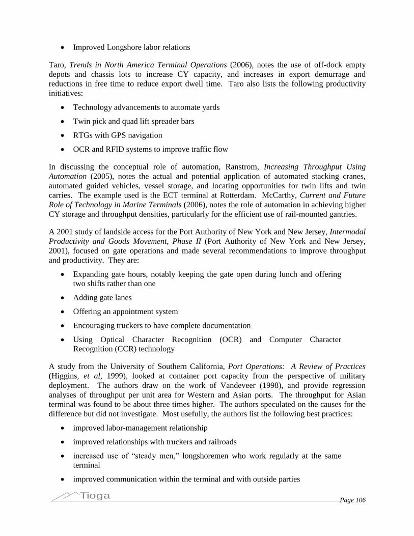
Page 106Tioga
Improved Longshore labor relations
Taro, Trends in North America Terminal Operations (2006), notes the use of off-dock emptydepots and chassis lots to increase CY capacity, and increases in export demurrage andreductions in free time to reduce export dwell time. Taro also lists the following productivityinitiatives:
Technology advancements to automate yards
Twin pick and quad lift spreader bars
RTGs with GPS navigation
OCR and RFID systems to improve traffic flow
In discussing the conceptual role of automation, Ranstrom, Increasing Throughput UsingAutomation (2005), notes the actual and potential application of automated stacking cranes,automated guided vehicles, vessel storage, and locating opportunities for twin lifts and twincarries. The example used is the ECT terminal at Rotterdam. McCarthy, Current and FutureRole of Technology in Marine Terminals (2006), notes the role of automation in achieving higherCY storage and throughput densities, particularly for the efficient use of rail-mounted gantries.
A 2001 study of landside access for the Port Authority of New York and New Jersey, IntermodalProductivity and Goods Movement, Phase II (Port Authority of New York and New Jersey,2001), focused on gate operations and made several recommendations to improve throughputand productivity. They are:
Expanding gate hours, notably keeping the gate open during lunch and offeringtwo shifts rather than one
Adding gate lanes
Offering an appointment system
Encouraging truckers to have complete documentation
Using Optical Character Recognition (OCR) and Computer CharacterRecognition (CCR) technology
A study from the University of Southern California, Port Operations: A Review of Practices(Higgins, et al, 1999), looked at container port capacity from the perspective of militarydeployment. The authors draw on the work of Vandeveer (1998), and provide regressionanalyses of throughput per unit area for Western and Asian ports. The throughput for Asianterminal was found to be about three times higher. The authors speculated on the causes for thedifference but did not investigate. Most usefully, the authors list the following best practices:
improved labor-management relationship
improved relationships with truckers and railroads
increased use of “steady men,” longshoremen who work regularly at the sameterminal
improved communication within the terminal and with outside parties
Page 107Tioga
improved information flow
automated gates
increased use of on-dock rail, although drawbacks were noted
Ward, Practical Port Productivity Measurement (1998), focuses on wharf and crane productivity,specifically the ability to handle ever-larger container ships. Ward lists multi-hoist, and multi-pick cranes as potential solutions, and these technologies have since been implemented at anumber of ports. The use of cranes on both sides, the so-called ship-in-a-slip (SIAS) system, isalso considered but that option is still theoretical.
Modeling and Theoretical Approaches
The importance and complexity of marine container terminal operations have led a number ofresearchers to explore various mathematical and statistical modeling approaches. Theseapproaches are primarily focused on the allocation of resources within the terminal itself. Theassignment of container cranes, yard gantries, and labor has received the most attention.Gonzalez and Trujillo, Efficiency Measurement in the Port Industry (2008), provide an extensivereview of the port efficiency modeling literature. They documented a wide range of approachesand results and a general lack of comparability due to differences in port types, productiondefinitions, and input variables. They also see a need for improved data collection.
Monteiro, Productivity and Efficiency Measurement in Ports (2009), provides a conceptualframework for modeling port productivity. Raw operational data (such as TEU handled or cranehours) are combined to form key performance indicators (KPIs). KPIs are typically ratios andinclude most of the performance metrics used or suggested by other authors, such as crane movesper hour. KPIs do not, however, specify a functional relationship, and Monteiro notes thatdifferent parties with different perspectives choose different KPIs. The next step is to developfunctional relationships, for which Monteiro considers three approaches: Price-based IndexFormulas, Stochastic Frontier Analysis (SFA), or Data Envelope Analysis (DEA).
Talley’s works on an overall economic model of a port, An Economic Theory of the Port (Talley,2006) and Port Performance: An Economics Perspective (Talley, 2007), extend the theoreticaltreatment beyond the terminal level. These treatments transcend the functional engineeringrelationships of berths, cranes, etc., to examine the mission of the port itself in maximizingthroughput and profit. As such, Talley examines demand as well as cost and production.
There have been several applications of Data Envelope Analysis to overall terminal productivity.Data Envelope Analysis (DEA) uses output data (in most cases, annual TEU) and a selection ofdependent variables to generate a “DEA Score” for each production unit, in this case a port orterminal. The best scores define a data envelope akin to an economic production frontier. Lessfavorable scores indicate relatively inefficient resource use, unrealized economies of scale, orother shortfalls.
There may also be some confusion due to the researcher’slack of experience with the containerterminal industry. Kaiser, et al, Efficiency Measurement of US Ports Using Data EnvelopmentAnalysis (2006), analyzed ro-ro terminals on the same basis as dedicated container crane
Page 108Tioga
terminals, and apparently used incorrect data for acreage at the Port of Long Beach. Turner, etal, North American Containerport Productivity 1984-1997 (2004), found it surprising that largervessels led to higher productivity, and that the presence of on-dock rail reduced overallthroughput per acre, both points that are obvious to industry participants.
Turner, et al, (2004) uses DEA with time-series data from 1984 to 1997. They conclude thatcontainer ports exhibit economies of scale, and identify rail access and service as a “critical determinant of container port infrastructure productivity.” Unfortunately, they do not delve intothe common metrics for terminal operation. The link they found between rail access and portthroughput may be attributable instead to the size of the market being served, which in turnexplains the presence of multiple railroads. Wang, Cullinane, and Song, Container PortProduction Efficiency: A Comparative Study of DEA and FDH Approaches (2003), comparedapproaches to port production efficiency using DEA and a Free Disposal Hull (FDH) Model.They found that different modeling techniques led to different conclusions, and that the use oftime-series or panel data would be more productive than using cross-section data. These authorsalso examine previous efforts to apply DEA or other techniques to the port productivity issue.
Poitras, et al, Measuring Port Efficiency: An Application of Data Envelopment Analysis (1996),use DEA to develop an efficiency ranking of 23 international ports. They found that theefficiency rankings varied with methodology but that DEA was a promising approach. Anotherapplication of DEA to container terminals, An Application of DEA Windows Analysis toContainer Port Production Efficiency (Cullinane, et al, 2004) took the time factor into accounton the grounds that port efficiency should change (and presumably improve) over time. Theauthors used several years of data from Asian ports, Long Beach, NY/NJ, and European ports.The study used quay length, terminal area, number of container cranes, number of yard gantries,and number of straddle carriers as land and equipment input proxies, and a pre-determinedrelationship between labor and terminal facilities. Unfortunately, this approach leaves theanalysis vulnerable to differences in terminal technology (e.g., wheeled terminals at Long Beachversus stacked terminals elsewhere) and significant variations in manning practices. In contrastto other studies, Cullinane, et al, found no economies of scale. The paper states that “the ports measured as being highly efficient appear to be those that do not actively invest over time.”Theauthors thus seem to have confirmed that terminals that do not expand must make greater use ofthe land and equipment they have. The authors conclude that “existing programming methods for estimating efficiency are inadequate in capturing the long-term increased efficiency andcompetitiveness that accrue for significant investments.”
Notteboom, et al, Measuring and Explaining the Relative Efficiency of Container Terminals byMeans of Bayesian Stochastic Frontier Models (2000), applied Stochastic Frontier modelingtechniques to a sample of 36 European and 4 Asian container ports. The study reported a higherdegree of efficiency in hub ports than in feeder ports. Liu, et al, Container Port Productivity andPort Policy Evaluation (2009), expect to use Stochastic Frontier Analysis (SFA) and MarkovChain Monte Carlo methods. The authors create a Port Operator Efficiency Index, but individualports are not identified.
The apparent limitation on the consistent use of DEA or other analytic techniques is thevariability and relevance of inputs. Authors have used inputs ranging from cargo uniformity anddepreciation charges to berth length and the number of tugs, few of which are under the control

Page 109Tioga
of terminal developers or managers. Of the two widely used DEA models, the “CCR” (Charnes, Cooper, and Rhodes) version assumes consistent returns to scale, which does not correspond tothe realities of container port development or operation. As terminals increase in scale, thebinding constraint on their capacity and productivity will shift from resource to resource, andthey will change production functions as they progress from low-cost, low-density operations tohigh-cost, high-density operations. As an example, Liu et al found that the DEA-CCR, DEA-BCC models indicated that Los Angeles and Long Beach (terminal unspecified) were moreefficient than Rotterdam, Hamburg, or some of the Hong Kong terminals. The FDH modelfound that most of the ports and terminals examined had equally high efficiency and wouldtherefore be of limited utility as an analytic tool. The DEA “BCC” variation returns to scale and may be more suitable.
While DEA may be a promising theoretical approach, studies reviewed to date provide onlylimited practical insight. The studies confirm the existence of economies of scale in containerterminal operations, but the existence of scale economies was never in doubt. The DEA studiesmay have been limited by their use of port-wide output data and characteristics, rather thanterminal-specific information. The choice of dependent variables may also limit the practicalapplication of studies. The researchers used port leasing policy, berth occupancy, the availabilityof double-stack clearances, and other factors as dependent variables only to find theminsignificant in the analysis. Sharma and Song, Performance Based Stratification and Clusteringfor Benchmarking of Container Terminals (2009), suggest combining DEA with data miningtechniques to create a better diagnostic tool.
The efforts to model container terminal production frontiers using DEA or related techniquesface some basic obstacles. At any given time, terminals almost certainly have a suboptimalcombination of production resources. Terminals do not have effective short-run control over theland area available, and cannot adjust their acreage to match demand. Berth length and channeldepth are likewise fixed in the short run, and often for the long run as well. Adding a newcontainer crane is a multi-year, multi-million dollar proposition. Even yard lift equipment, suchas RTGs or straddle carriers, requires a substantial investment and lead time. In the short run,labor is almost the only variable input.
The multiple efforts at modeling container port performance illustrate a classic dilemma: thedata available to modelers often lack explanatory power, and data more directly related toefficiency are inaccessible or confidential. The modelers are thus in the difficult position oftrying to identify a production frontier using variables that are secondary or tertiary at best. Theliterature confirms this problem in a round-about way by concluding that many of the variablesused have no explanatory power, that better data are needed, and that the modeling effort overallis in an early stage of development.
End Notes
In addition to the sources reviewed above there are a number of other potentially useful articlesand presentations on port productivity and related subjects. Literature reviews are included inmost of the publications cited above, notably Wang, et al, Container Port Production Efficiency:A Comparative Study of DEA and FDH Approaches (2003). An extensive review of theliterature on port economics is contained in Pallis, et al, Port Economics, Policy and

Page 110Tioga
Management –Review of an Emerging Research Field (2009), a work reviewed in draft andpublished in Transport Reviews, 2009.
The great majority of the sources above are obtainable in full text versions and are being madeavailable on Tioga’s FTP site for use in this project. A few, however, were only obtainable inabstract or executive summary form and are so indicated in the references listing.

Page 111Tioga
References
Papers and Articles
Ashar, A., 1985. Productivity and Capacity of Container Terminals. World Wide Shipping,October/November.
Ashar, A., 1997. Port Productivity Revisited, Port Development International, November.
Beŝkovnik, B, 2008. Measuring and Increasing the Productivity Model on Maritime ContainerTerminals, Pomorstvo, god. 22, br. 2, pp. 171-183.
Chen, C., Hsu, W-J., and Huang, S-Y., 2003. Simulation and Optimization of Container YardOperations: A Survey. Center for Advanced Information Systems, School of ComputerEngineering, Nanyang Technological University, Singapore.
Choi, Y.S., 2005. Analysis of Combined Productivity of Equipments in Container Terminal.(Publisher Unknown)
Chung, K., 1993. Port Performance Indicators. Transport No. PS-6. Transportation, Water andUrban Development Department, The World Bank.
Cullinane, K., Song, D-W, Ji, P., and Wang, T-F, 2004. An Application of DEA WindowsAnalysis to Container Port Production Efficiency. Review of Network Economics, Vol. 3, Issue2, June.
De Monie, G., 1987. Measuring and Evaluating Port Performance and Productivity. UNTADmonograph.
Fourgeaud, P., 2009. Measuring Port Performance. The World Bank, infoMARE Forum ofShipping and Logistics, September 25, 2009.
Gonzalez, M. and Trujillo, L., 2008. Efficiency Measurement in the Port Industry: A Survey ofthe Empirical Evidence. City University of London, Department of Economics, DiscussionPaper No. 07/07.
Henesey, L., 2004. Container Terminal Performance: A Multi-Agent Systems Approach.Blekinge Institute of Technology.
Henesey, L., Fredrik Wernstedt, F., Paul Davidsson, P., 2003. Market-Driven Control inContainer Terminal Management. Blekinge Institute of Technology, Ronneby/ Sweden.
Itmi, M, Ndiaye, A, Maria, M, and Pruni, J, 2001. Simulating Operations Policies in aContainer Terminal. Korea Advanced Institute of Science and Technology, Systems ModelingSimulation Laboratory
Jeon, Y, and Park, Y-M., 2005. Status and Visions of Automated Container Terminals.Proceedings of the Fifteenth International Offshore and Polar Engineering Conference, pp. 656+.
Page 112Tioga
Kaisar, E., Pathomsiri, S., Haghani, A., 2006. Efficiency Measurement of US Ports Using DataEnvelopment Analysis. National Urban Freight Conference, February 1-3, 2006.
Le-Griffin, H. and Murphy, M., 2006. Container Terminal Productivity: Experiences at thePorts of Los Angeles and Long Beach. National Urban Freight Conference, February 1-3, 2006.
Leong, T-Y, and Lau, H, 2007. Generating Job Schedules for Vessel Operations in a ContainerTerminal. MISTA.
Liu, J., Yip, T., Yan, J., and Sun, X., 2009. Container Port Productivity and Port PolicyEvaluation. C. Y. Tung International Centre for Maritime Studies, Hong Kong PolytechnicUniversity (abstract).
Mongelluzzo, Bill, 2009. The Productivity Principle. The Journal of Commerce, October 19,pp. 23-24.
Notteboom, T, Coeck, C., and Van Den Broeck, J, 2000. Measuring and Explaining the RelativeEfficiency of Container Terminals by Means of Bayesian Stochastic Frontier Models.International Journal of Maritime Economics, no. 2, pp. 83-106 (abstract).
Pallis, A., Vitsounis, T., and De Langan, P. unpublished. Port Economics, Policy andManagement–Review of an Emerging Research Field. author’s version, http://dx.doi.org/10.1080/01441640902843208.
Poitras, G., Tongzon, J., and Li, H., 1996. Measuring Port Efficiency: An Application of DataEnvelopment Analysis. Department of Economics and Statistics, National University ofSingapore.
Sharma, M. and Song, J., 2009. Performance Based Stratification and Clustering forBenchmarking of Container Terminals. Expert Systems with Applications: An InternationalJournal Archive, volume 36, no. 3, April (abstract).
Talley, W., 2006. An Economic Theory of the Port. Research in Transportation Economics, vol.16, Elsevier, pp. 43-65.
Talley, W., 2007. Port Performance: An Economics Perspective. Research in TransportationEconomics, vol. 17, Elsevier, pp. 499-516.
Turner, H., Windle, R., and Dresner, M., 2004. North American Containerport Productivity:1984–1997. Transportation Research Part E: Logistics and Transportation Review, vol. 40, no.4, July, pp. 339-356
Vandeveer, D., 1998. Port Productivity Standards for Long-term Planning. Ports’98, American Society of Civil Engineers, vol. 1, pp. 79-88 (hardcopy).
Wang, T., Song, D. W. and Cullinane, K., 2002. The Applicability of Data EnvelopmentAnalysis to Efficiency Measurement of Container Ports. Proceedings of the InternationalAssociation of Maritime Economists Conference, Panama, 13-15 November.
Page 113Tioga
Wang, T-F., Cullinane, K., and Song, D-W., 2003. Container Port Production Efficiency: AComparative Study of DEA and FDH Approaches. Journal of the Eastern Asia Society forTransportation Studies, vol. 5, October, pp. 698-713.
Ward, T., 1998. New Ideas for Increasing Wharf Productivity. Ports ’98, American Society of Civil Engineers, vol. 1, pp. 69-78
Presentations
Isbell, J., 2005. Satisfying the Needs of the Port’s Clients. Presentation to the Marine TerminalManagement Training Program, where?.
McCarthy, E., 2006. Current and Future Role of Technology in Marine Terminals. Presentationto the Marine Terminal Management Training Program, Long Beach.
Monteiro, F, 2009. Productivity and Efficiency Measurement in Ports. Presentation to the PortProductivity Conference
Nye, L., 2009. Advanced Technology in Terminal Design. PowerPoint presentation,
Olivier, D., 2009. Developing Utilization Indicators for Canadian Ports. Presentation to the2009 Port Productivity Conference.
Ranstrom, J., 2005. Increasing Throughput Using Automation. Presentation to the MarineTerminal Management Training Program.
Rugaihuruza, J., 2007. Infrastructure, Operational Efficiency and Port ProductivityManagement in PMAESA Region. Presentation to the African Ports/Maritime Conference,December.
Schmidmeir, G., undated. Leveraging Technology to Boost Port Productivity. NavisPowerPoint presentation.
Tarkenton, L., 2005. Trends in Marine Terminal Operations Management. Presentation to theMarine Terminal Management Training Program, Long Beach
Taro, N., 2006. Trends in North American Terminal Operations. Presentation to the MarineTerminal Management Training Program
Ward, T., 2000. Practical Port Productivity Measurement. Presentation, Vera Cruz, March 21.
Reports
Atkins, W., 1983. Modern Marine Terminal Operations and Management. Port of Oakland(book).
Australia Productivity Commission, 2003. International Benchmarking of ContainerStevedoring. Commission Research Paper, July.
Page 114Tioga
Bureau of Transport Economics (Australia), 1984. Container Terminal Productivity in PortJackson from 1977 to 1981.
Committee on Productivity of Marine Terminals, 1986. Improving Productivity in U.S. MarineContainer Terminals. Marine Board, National Research Council (Executive Summary).
Cornell Group, Inc., 2007. Container Terminal Parameters. Maine Department ofTransportation.
HK Economic Development and Labour Bureau, 2004. Study on Hong Kong Port–Master Plan2020. Draft Executive Summary, Annex.
Hanam Canada Corporation, 2007. Container Capacity Expansion Plans at Pacific Coast Ports.Policy Research Branch, Strategic Policy Directorate, Policy Group, Transport Canada.
Hanam Canada Corporation, 2008. Pacific Coast Container Terminal Competitiveness Study.Policy Research Branch, Strategic Policy Directorate, Policy Group, Transport Canada.
Higgins, T, Dessouky, M., Hall, R, 1999. Port Operations: A Review of Practices. Center forCommercial Deployment of Transportation Technologies, University of Southern California,Center for Advanced Transportation Technologies.
JWD Group, 2003. U.S. Container Terminal Throughput Density. Report to the Port of HoustonAuthority.
JWD Group, 2004. Maritime Development Alternatives Study. Prepared for the Port of Oakland.
JWD Group, 2006. Port of Long Beach Terminal Capacity Analysis. Report to the PortAuthority of Long Beach.
NETS, 2006. New Measures of Port Efficiency Using International Trade Data. U.S. ArmyCorps of Engineers, Navigation-Economics-Technologies Program, IWR Report 06-NETS-R-01.
Parsons Brinckerhoff, 2009. Strategic Advisory Report: Napoleon Avenue Container TerminalDevelopment Utilizing Public-Private Partnerships. Prepared for The Board of Commissionersof the Port of New Orleans.
Port Authority of New York and New Jersey, 2001. Intermodal Productivity and GoodsMovement, Phase II: Land Access to Port and Terminal Gate Operations.
Tioga Group, 2009. SF Bay Area Containerized Cargo Outlook. Prepared for the San FranciscoBay Conservation and Development Commission.
US DOT, 2009. America’s Container Ports: Freight Hubs That Connect Our Nation to Global Markets. U.S. Department of Transportation, Research and Innovative TechnologyAdministration, Bureau of Transportation Statistics.

Page 115Tioga
Appendix B: Insights from Rail Intermodal Terminals
Objective
The objective of this Appendix is to document the historical and current patterns of railintermodal terminal development, identify those patterns that are most applicable to the marineport industry, and to draw conclusions useful for the marine terminal productivity study.
Rail terminal efficiency is measured by cost per lift, with a lift being the transfer between railand highway modes. Measures of physical productivity are subordinate and managed with thegoal of influencing the cost per lift.
An emerging theme of this Port Productivity Study is that the treatment of land costs is a key tounderstanding the development patterns, planning decisions, and subsequent productivity atmarine terminals. The relatively low cost of land in the U.S. leads to efficient facility designsand operational practices that use much more land than terminals in major Asian or Europeancities.
The development pattern of United States rail intermodal terminals shares some of the samecharacteristics with marine terminals; therefore, as part of the larger examination of marineterminal productivity and productivity measurement, Tioga analyzed the development patterns ofrail intermodal facilities and identified their implications for the marine terminals that are theprimary subject of this study.
To illustrate the financial implications of current rail development options and show how landcosts strongly influence that development, Tioga modeled the cost of six hypothetical scenarios.These scenarios illustrate how terminal cost per lift increases as the cost of land increases; andhow that increase can be mitigated through the use of stacking, coupled with capital equipment,and technologies that drive scale economies.
Background
In 2006 North American railroads moved 14,234,0743 intermodal loads in containers and trailersthrough approximately 225 intermodal terminals.4 The function of the intermodal terminals is totransfer the container or trailer between modes. Each transfer is called a lift. In 2006, there weremore than 30 million lifts performed in North American rail terminals.5
Rail intermodal terminals and marine terminals are functionally very similar. The maindifference is that the“berth”in a rail intermodal terminal is a set of railroad tracks which can be
3 http://www.intermodal.org/statistics_files/stats1.shtml4 225 is the approximate number in the IANA data set. There are a few identifiable duplicates in IANA’s data, and the data set does not include
some smaller terminals or on-dock rail intermodal terminals.5 There is at least one lift at each end of a loaded movement. In addition, there are movements of empty equipment, and some loads are lifted
more than twice.

Page 116Tioga
served by a side loader or gantry crane. Rail terminals lift both trailers and containers. Trailerswere previously rolled on and off rail cars, but this practice has largely been replaced. On therailroad a switch engine moves the loaded train to/from the loading tracks. In a marine operationthis function is performed by a maritime tug. Beyond these apparent differences, the clerical,gate, and container yard functions are very similar. The lift equipment and yard tractors arenearly identical.
Overview of Rail Terminal Services
Lifts. Activity at intermodal terminals is most commonly measured in lifts. A lift is the transferof a trailer or container from a rail car to the ground/chassis, or from the ground/chassis to railcar. Often there is a service component. Typically, outbound trailers and containers arrivingprior to an agreed cut-off time must be lifted to a train prior to a scheduled release time. Inboundtrailers and containers must be lifted off the train (grounded) and made available for drayagewithin a specific time window, often 2 hours.
Contract terminal operators are typically paid based on the number of primary lifts they perform.In most terminals, lifts are counted by shift. Some terminal operators distinguish betweenprimary and secondary lifts. A primary lift is a lift to/from a rail car. A secondary lift is betweena chassis and a stack.
Gate transactions. While lifts is the measure of activity for the rail side of the intermodalterminal, gate transactions is the measure of activity for the highway mode. Trucks enter andleave the terminal to deliver and pick up loaded and empty trailers and containers. The truckflow through the terminal can be used as a demand/work measure for gate and clerical personnel.It can also be used to identify the impact on traffic through a determination of a gate activity/liftratio (typically 1.5 gate transactions for every 1 lift).
The daily cycle. Terminals typically strive to match shipper practices. For many facilities, thismeans handling inbound trains in the morning and outbound trains in the afternoon or evening.This cycle is less pronounced at the largest terminals and those in the middle of a network.
The weekly cycle. Most customers ship five or six days per week. Most rail intermodalterminals work six or seven days per week because trains move seven days per week.Intermodal terminals, therefore, handle most outbound traffic Monday through Friday. A smallminority are handled on Saturdays, and an even smaller portion of the outbound are handled onSundays. Inbound traffic flows into the terminal all weekend. Generally, it is unloadedthroughout the weekend in order to make it available to customers, most of whom want thetraffic Monday morning. The weekly cycle strongly influences the rail car and trailer storagerequirements.
Annual cycle. Generally, intermodal terminals have relatively small seasonal peaks in Marchand October, and have a significant low period in late December and early January.
Intermediate “hub” terminals. Intermodal movement from shipper to receiver often involveshandling at intermediate terminals. For example, in Los Angeles, international intermodalshipments move between marine terminals and intermodal terminals over the highways.

Page 117Tioga
Domestic transcontinental shipments that must change railroads are often handled the same wayin gateway cities, such as Chicago. Terminals that provide these services have cycles andpeaking characteristics influenced/driven by the unique demands of the interchange traffic.
End-point terminals. End-point terminals, with little impacted from intermediate movements,experience shipper driven cycles and peaks. End-point terminals require larger parking lots tobuffer weekend-driven demand peaks.
Supplying Rail Terminal Services
Most rail intermodal terminals are owned by railroads.6 As with marine transportation, the costof rail intermodal terminal operations is bundled into the point-to-point transportation rate. Railcustomers typically do not see a separate accounting for terminal costs.
Sub-contracting practices vary widely in the rail industry. In Canada and in some U.S. facilities,100% of the work is performed by rail employees. It is more common, however, for a U.S.intermodal terminal to operate with a combination of rail and contractor employees.
Regardless of the status of their employers, in a railroad terminal, there are typically threefunctional categories of labor: yard workers, clerks, and mechanics. Yard workers drive the yardtractors and lift equipment. They also serve as ground men working the hitches and interboxconnectors. Mechanics are further subdivided into those who work on powered equipment andthose who work on trailers, containers, and chassis. In a heavily unionized environment, eachcategory may be represented by a different union. In smaller and nonunion environments, thedistinctions between supervisors and labor are blurred as are the distinctions between functionallabor categories. In very small terminals, a yard worker may unload a trailer and then drive thedrayage truck that delivers it to the customer.
In the United States, there are several intermodal terminal operating companies that provideintermodal terminal services, up to and sometimes including operating switch engines. Many ofthese services are sold on the basis of a price per lift because it is accepted as a fair measure ofterminal activity. When railroads offer to subcontract terminal services, they prepare a Requestfor Proposal that outlines the menu of services that are to be contracted. There is absolutely no“standard package” of services; each and every procurement is unique.
The menu may include:
Labor to make the transfer, store, and retrieve the unit in the yard. In most, butnot all locations, the tie down labor is included.
Labor to check units in and out of the gate and perform clerical functions. It isrelatively more common for the railroad to provide its own clerical services.
Labor to maintain the equipment.
6 On dock rail intermodal facilities are the most common exception. These are typically owned by the port, leased to the marine terminal
operator, and staffed with less flexible Longshore labor.
Page 118Tioga
Allocated capital costs of mobile equipment (lift equipment, yard tractors, andancillary vehicles). Almost always the terminal operator provides yard tractorsand ancillary vehicles; more often than not, the railroad provides the liftequipment.
Fuel, utility, and other supply costs.
Information systems and communications costs.
Liability for accidents, regardless of responsibility.
Rarely, railroads will select a “turn-key” operation for their intermodal facilities. In this case, thecontractor provides all of the equipment, sometimes including the switch engine. The onlypersonnel on the terminal, including security, may be contractor employees.
Tioga is not aware of any example of a design/build/operate arrangement using railroad-ownedland, though there has been some discussion of this approach. In this case, an outside partywould perform not only a turnkey operational service, but also finance and build the facility.
Finally, there is a significant minority of private and on-dock terminals, which are not owned byrailroads. These are typically operated by rail intermodal terminal operators and marinestevedoring firms. In these cases, the entire terminal function can be said to be subcontracted.
Rail versus Marine Container Moves
Almost all U.S. rail intermodal terminals are wheeled, with containers parked on chassis ratherthan stacked or grounded. Each container transaction, inbound or outbound, ordinarily consistsof a single lift between chassis and rail car. Secondary lifts or “flips” are rare and are often discouraged with high assessorial charges.
Almost all major U.S. marine terminals are hybrids, with many or most loaded containersstacked. A container transaction involving stacked containers requires at least three lifts. For animport box, for example, there will be at least three:
one from the vessel to a yard chassis;
one from the yard chassis to a stack; and
one from the stack to a road chassis.
In marine terminal straddle carrier operations there would also be at least three:
one from vessel to ground at the apron;
one from the apron to the CY; and
one from the CY to the road chassis.

Page 119Tioga
In any stacked operation, there is also the possibility of additional lifts to sort the stack or to getto the desired box. Where import loads are wheeled, there should be only a single lift from thevessel to the road chassis. As a result, marine terminals (or grounded rail intermodal terminals)spend more capital on lift equipment.
Rail Terminal Productivity Measures
Railroad terminal operators tend to look and measure terminal productivity in a number ofdifferent ways based on the time horizon in question. The daily issue at an intermodal terminalis how many people and machines are needed for the next shift. There is generally much morelabor flexibility in rail intermodal terminals than in port operations. The terminal operator canmost often decide which of his employees will operate lift equipment and which will performother job responsibilities, such as yard driver or tiedown person.
The question is answered based on an estimate of workload for the shift, coupled withknowledge of the equipment and the skill level of individual workers. At the level of the shiftsupervisor, the “who” is the most important question. The workload is estimated based on the certain knowledge of the volume and schedule status of inbound trains and an estimate ofoutbound business volumethat will arrive at the terminal prior to “cut off.” Some railroads issuereservations; others talk to customers (“UPS has 55 coming tonight”) to improve the quality of these estimates. At this level, productivity measures, such as lifts per man hour and productivityrates for individual operators, are used to size the crews.
Planners with a longer time horizon are typically more interested in longer-term productivityissues involving investments in land, equipment, and facilities. Often these individuals areinvolved in capital investment decisions. To measure performance and support this kind ofanalysis, railroads and their contractors rely on a number of standard performance measures.
Rail Terminal Performance Measures
Facility Measures. These measures typically compare the annual lift count to the portions of thefacility. Lifts per track space (or foot of track), lifts per parking space, and lifts per acre arecommonly used measures.
Equipment Measures. Equipment productivity is measured in terms of lifts per time period(shift, day, month, and year). More important, though, is schedule compliance. Regardless oflong-term efficiency, a terminal needs enough operational equipment to meet the peak demandsimposed by the train schedule and associated customer commitments.
Labor Measures. Labor productivity varies widely. The most common labor specializations inan intermodal terminal are drivers (heavy equipment and yard tractors), mechanics, and clerks.In some places each trade is represented by a different union. In other locations workers are notunionized and are cross-trained between specializations. In some locations the distinctionbetween labor and management may not be obvious. In addition, terminals are often staffed by amix of contractor, railroad, and railroad subsidiary employees. The most common measurescompare lifts or gate transactions with payroll. Lifts per man-hour and staff minutes per gatetransaction are also common measures.

Page 120Tioga
Rail Intermodal Terminal Development
While the origins of the rail intermodal freight industry can be traced back to the loading ofcircus wagons on rail flat cars more than a century ago, modern Trailer on Flat Car (TOFC)service is a post-World War II phenomenon. Railroads advanced the business in order to stemmarket share losses to motor carriers, which were accelerated by the construction of theInterstate Highways.
In the early years, most terminals made the mode transfer by driving the trailers onto ordinaryflat cars. This was called “circus” loading, after the way in which circus wagons were loadedonto railroad flatcars in the 1800s. Terminals were cheap to build and could achieve nearoptimal efficiency with relatively low volumes. As a result, intermodal terminals proliferated andalmost every medium-sized (and larger) community in the US had a simple intermodal terminal,usually called a “piggy back” ramp. These facilities were usually built on the edges of existing freight or passenger facilities. The low profit margins on early rail TOFC/COFC business wouldrarely have justified the purchase of land.
To address the problem of low profit margins, railroads found that they could improveintermodal service by operating dedicated intermodal trains between major city pairs. Stoppingat every medium-sized city en-route slowed the trains to a point that service becameuncompetitive and rates became unprofitable. Intermodal service to these communities actuallyimproved when local piggyback ramps were closed, as traffic was drayed to a “hub” location in a major city that could load the freighton a dedicated intermodal “through” train.
Furthermore, beginning in the 1960s, it became possible to operate a terminal at a much lowercost by lifting the trailers or containers on and off the rail cars. The capital cost of the heavylifting equipment and the paved surface to support it was high, requiring a relatively largevolume of traffic to gain this efficiency. It was also subsequently determined that a large amountof tare weight could be taken out of flat cars if they did not need to be strong enough for heavytrucks to drive on. These economic factors made intermodal service viable only in the largestcities, and resulted in the abandonment of many small- and medium-sized facilities.
In the late 1960s and early 1970s, there were a number of “side-by-side” rail mergers. The associated facility rationalization led to an additional decline in the number of terminals. Forexample, on Conrail, which was formed in 1976 from the bankrupt northeastern railroads, thecombination of these factors caused the number of terminals to decline from 40 to 24 between1979 and 1984.
Since 1975, rail intermodal volume has grown dramatically. To adequately manage thisrelatively rapid, long-term growth, most railroads have focused their available capital andmanagement attention on easily served, long-haul, high-density corridors. This emphasis haslimited intermodal traffic, to traffic lanes between large cities in which all of the major railroadsinvolved have a long haul (500 miles or more). Even given this restrictive strategy, railroadshave been adding roughly 500 acres of new intermodal terminal capacity each year to keep pacewith growth.
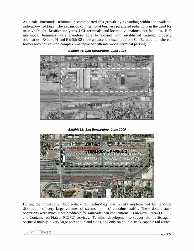
Page 121Tioga
As a rule, intermodal terminals accommodated this growth by expanding within the availablerailroad-owned land. The expansion of intermodal business paralleled reductions in the need formassive freight classification yards, LCL terminals, and locomotive maintenance facilities. Railintermodal terminals were therefore able to expand with established railroad propertyboundaries. Exhibit 91 and Exhibit 92 show an excellent example from San Bernardino, where aformer locomotive shop complex was replaced with intermodal terminal parking.
Exhibit 91: San Bernardino, June 1994
Exhibit 92: San Bernardino, June 2009
During the mid-1980s, double-stack rail technology was widely implemented for landsidedistribution of very large volumes of steamship lines’container traffic. These double-stackoperations were much more profitable for railroads than conventional Trailer-on-Flatcar (TOFC)and Container-on-Flatcar (COFC) services. Terminal development to support this traffic againoccurred mainly in very large port and inland cities, and only on double-stack-capable rail routes.
LOCOMOTIVE SHOPS
INTERMODAL PARKING
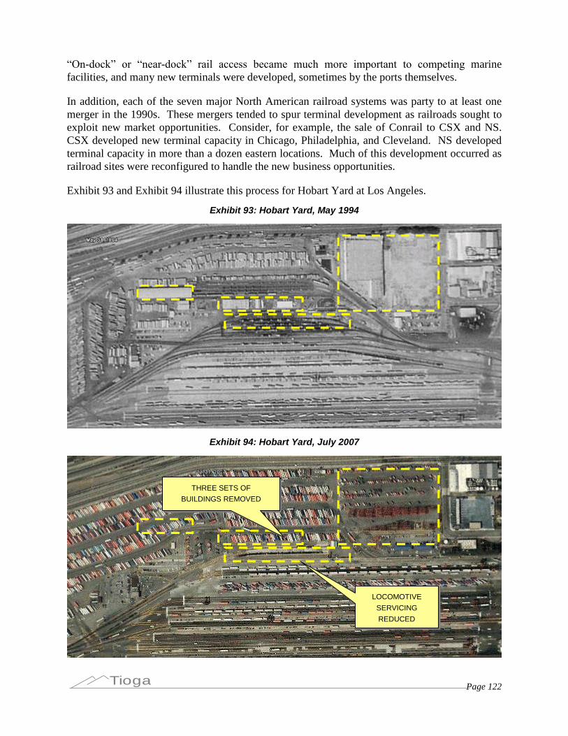
Page 122Tioga
“On-dock” or “near-dock” rail access became much more important to competing marinefacilities, and many new terminals were developed, sometimes by the ports themselves.
In addition, each of the seven major North American railroad systems was party to at least onemerger in the 1990s. These mergers tended to spur terminal development as railroads sought toexploit new market opportunities. Consider, for example, the sale of Conrail to CSX and NS.CSX developed new terminal capacity in Chicago, Philadelphia, and Cleveland. NS developedterminal capacity in more than a dozen eastern locations. Much of this development occurred asrailroad sites were reconfigured to handle the new business opportunities.
Exhibit 93 and Exhibit 94 illustrate this process for Hobart Yard at Los Angeles.
Exhibit 93: Hobart Yard, May 1994
Exhibit 94: Hobart Yard, July 2007
THREE SETS OFBUILDINGS REMOVED
LOCOMOTIVESERVICINGREDUCED
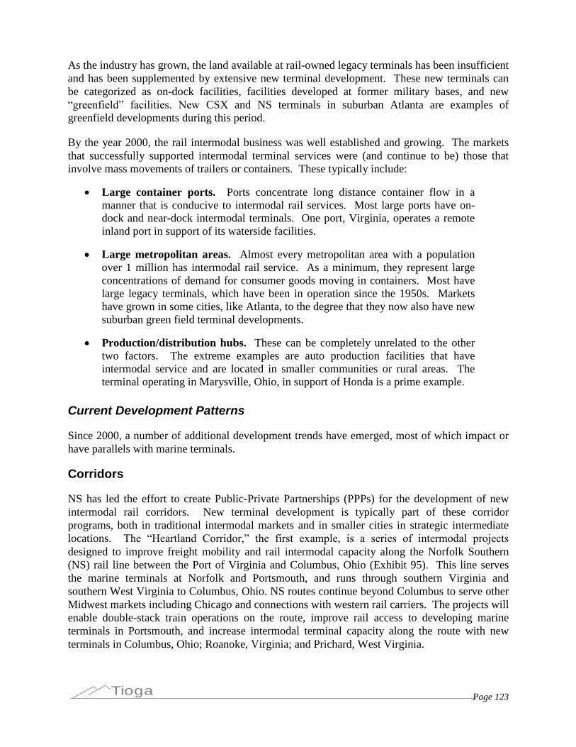
Page 123Tioga
As the industry has grown, the land available at rail-owned legacy terminals has been insufficientand has been supplemented by extensive new terminal development. These new terminals canbe categorized as on-dock facilities, facilities developed at former military bases, and new“greenfield” facilities. New CSX and NS terminals in suburban Atlanta are examples ofgreenfield developments during this period.
By the year 2000, the rail intermodal business was well established and growing. The marketsthat successfully supported intermodal terminal services were (and continue to be) those thatinvolve mass movements of trailers or containers. These typically include:
Large container ports. Ports concentrate long distance container flow in amanner that is conducive to intermodal rail services. Most large ports have on-dock and near-dock intermodal terminals. One port, Virginia, operates a remoteinland port in support of its waterside facilities.
Large metropolitan areas. Almost every metropolitan area with a populationover 1 million has intermodal rail service. As a minimum, they represent largeconcentrations of demand for consumer goods moving in containers. Most havelarge legacy terminals, which have been in operation since the 1950s. Marketshave grown in some cities, like Atlanta, to the degree that they now also have newsuburban green field terminal developments.
Production/distribution hubs. These can be completely unrelated to the othertwo factors. The extreme examples are auto production facilities that haveintermodal service and are located in smaller communities or rural areas. Theterminal operating in Marysville, Ohio, in support of Honda is a prime example.
Current Development Patterns
Since 2000, a number of additional development trends have emerged, most of which impact orhave parallels with marine terminals.
Corridors
NS has led the effort to create Public-Private Partnerships (PPPs) for the development of newintermodal rail corridors. New terminal development is typically part of these corridorprograms, both in traditional intermodal markets and in smaller cities in strategic intermediatelocations. The “Heartland Corridor,” the first example, is a series of intermodal projects designed to improve freight mobility and rail intermodal capacity along the Norfolk Southern(NS) rail line between the Port of Virginia and Columbus, Ohio (Exhibit 95). This line servesthe marine terminals at Norfolk and Portsmouth, and runs through southern Virginia andsouthern West Virginia to Columbus, Ohio. NS routes continue beyond Columbus to serve otherMidwest markets including Chicago and connections with western rail carriers. The projects willenable double-stack train operations on the route, improve rail access to developing marineterminals in Portsmouth, and increase intermodal terminal capacity along the route with newterminals in Columbus, Ohio; Roanoke, Virginia; and Prichard, West Virginia.
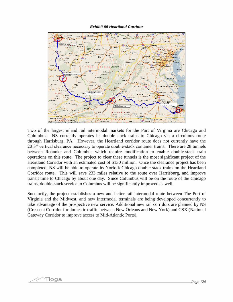
Page 124Tioga
Exhibit 95 Heartland Corridor
Two of the largest inland rail intermodal markets for the Port of Virginia are Chicago andColumbus. NS currently operates its double-stack trains to Chicago via a circuitous routethrough Harrisburg, PA. However, the Heartland corridor route does not currently have the20’3” vertical clearance necessary to operate double-stack container trains. There are 28 tunnelsbetween Roanoke and Columbus which require modification to enable double-stack trainoperations on this route. The project to clear these tunnels is the most significant project of theHeartland Corridor with an estimated cost of $130 million. Once the clearance project has beencompleted, NS will be able to operate its Norfolk-Chicago double-stack trains on the HeartlandCorridor route. This will save 233 miles relative to the route over Harrisburg, and improvetransit time to Chicago by about one day. Since Columbus will be on the route of the Chicagotrains, double-stack service to Columbus will be significantly improved as well.
Succinctly, the project establishes a new and better rail intermodal route between The Port ofVirginia and the Midwest, and new intermodal terminals are being developed concurrently totake advantage of the prospective new service. Additional new rail corridors are planned by NS(Crescent Corridor for domestic traffic between New Orleans and New York) and CSX (NationalGateway Corridor to improve access to Mid-Atlantic Ports).
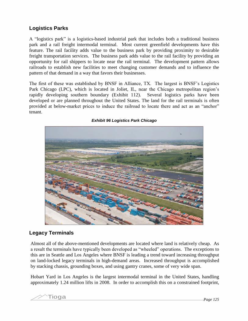
Page 125Tioga
Logistics Parks
A “logistics park” is a logistics-based industrial park that includes both a traditional businesspark and a rail freight intermodal terminal. Most current greenfield developments have thisfeature. The rail facility adds value to the business park by providing proximity to desirablefreight transportation services. The business park adds value to the rail facility by providing anopportunity for rail shippers to locate near the rail terminal. The development pattern allowsrailroads to establish new facilities to meet changing customer demands and to influence thepattern of that demand in a way that favors their businesses.
The first of these was established by BNSF in Alliance, TX. The largest is BNSF’s Logistics Park Chicago (LPC), which is located in Joliet, IL, near the Chicago metropolitan region’s rapidly developing southern boundary (Exhibit 112). Several logistics parks have beendeveloped or are planned throughout the United States. The land for the rail terminals is oftenprovided at below-market prices to induce the railroad to locate there and act as an “anchor” tenant.
Exhibit 96 Logistics Park Chicago
Legacy Terminals
Almost all of the above-mentioned developments are located where land is relatively cheap. Asa result the terminals have typically been developed as “wheeled” operations.The exceptions tothis are in Seattle and Los Angeles where BNSF is leading a trend toward increasing throughputon land-locked legacy terminals in high-demand areas. Increased throughput is accomplishedby stacking chassis, grounding boxes, and using gantry cranes, some of very wide span.
Hobart Yard in Los Angeles is the largest intermodal terminal in the United States, handlingapproximately 1.24 million lifts in 2008. In order to accomplish this on a constrained footprint,
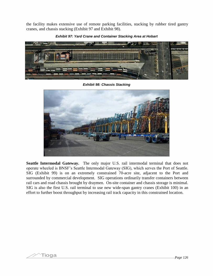
Page 126Tioga
the facility makes extensive use of remote parking facilities, stacking by rubber tired gantrycranes, and chassis stacking (Exhibit 97 and Exhibit 98).
Exhibit 97: Yard Crane and Container Stacking Area at Hobart
Exhibit 98: Chassis Stacking
Seattle Intermodal Gateway. The only major U.S. rail intermodal terminal that does notoperate wheeled is BNSF’s Seattle Intermodal Gateway (SIG), which serves the Port of Seattle.SIG (Exhibit 99) is on an extremely constrained 70-acre site, adjacent to the Port andsurrounded by commercial development. SIG operations ordinarily transfer containers betweenrail cars and road chassis brought by draymen. On-site container and chassis storage is minimal.SIG is also the first U.S. rail terminal to use new wide-span gantry cranes (Exhibit 100) in aneffort to further boost throughput by increasing rail track capacity in this constrained location.
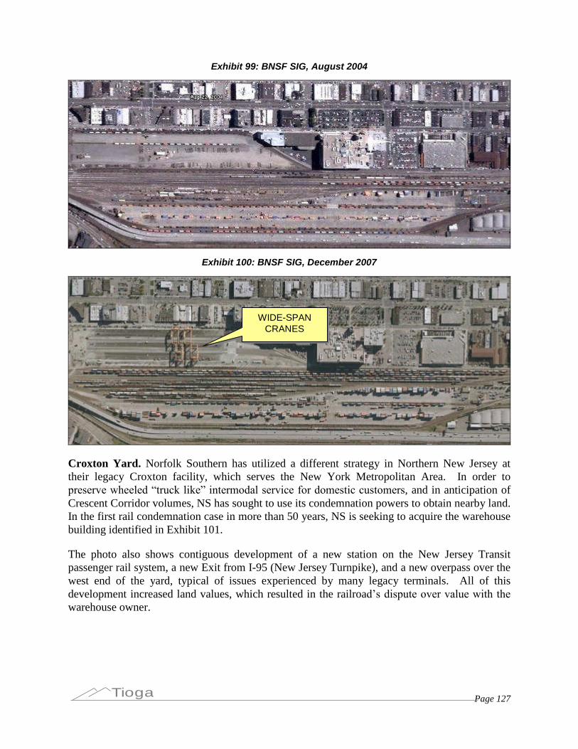
Page 127Tioga
Exhibit 99: BNSF SIG, August 2004
Exhibit 100: BNSF SIG, December 2007
Croxton Yard. Norfolk Southern has utilized a different strategy in Northern New Jersey attheir legacy Croxton facility, which serves the New York Metropolitan Area. In order topreserve wheeled “truck like” intermodal service for domestic customers, and in anticipation ofCrescent Corridor volumes, NS has sought to use its condemnation powers to obtain nearby land.In the first rail condemnation case in more than 50 years, NS is seeking to acquire the warehousebuilding identified in Exhibit 101.
The photo also shows contiguous development of a new station on the New Jersey Transitpassenger rail system, a new Exit from I-95 (New Jersey Turnpike), and a new overpass over thewest end of the yard, typical of issues experienced by many legacy terminals. All of thisdevelopment increased land values, which resulted in the railroad’s dispute over value with the warehouse owner.
WIDE-SPANCRANES
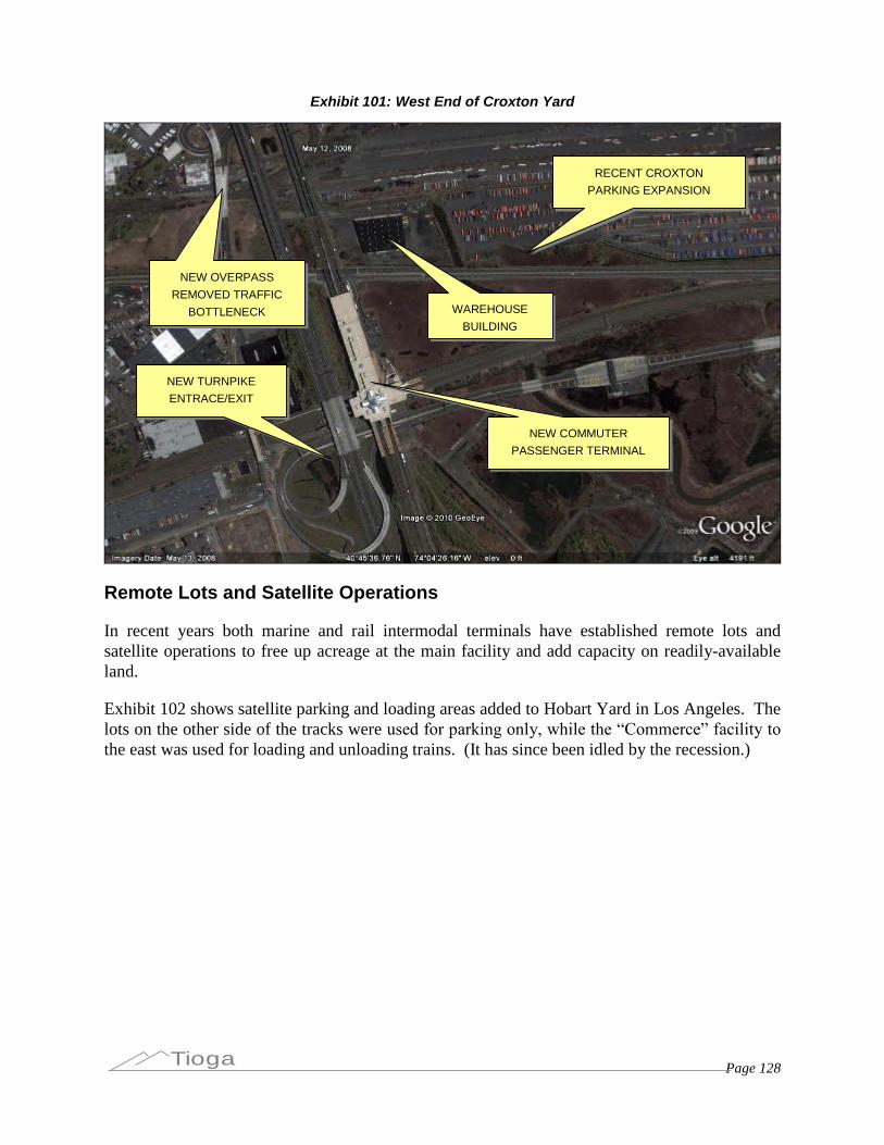
Page 128Tioga
Exhibit 101: West End of Croxton Yard
Remote Lots and Satellite Operations
In recent years both marine and rail intermodal terminals have established remote lots andsatellite operations to free up acreage at the main facility and add capacity on readily-availableland.
Exhibit 102 shows satellite parking and loading areas added to Hobart Yard in Los Angeles. Thelots on the other side of the tracks were used for parking only, while the “Commerce” facility to the east was used for loading and unloading trains. (It has since been idled by the recession.)
WAREHOUSEBUILDING
RECENT CROXTONPARKING EXPANSION
NEW COMMUTERPASSENGER TERMINAL
NEW OVERPASSREMOVED TRAFFIC
BOTTLENECK
NEW TURNPIKEENTRACE/EXIT
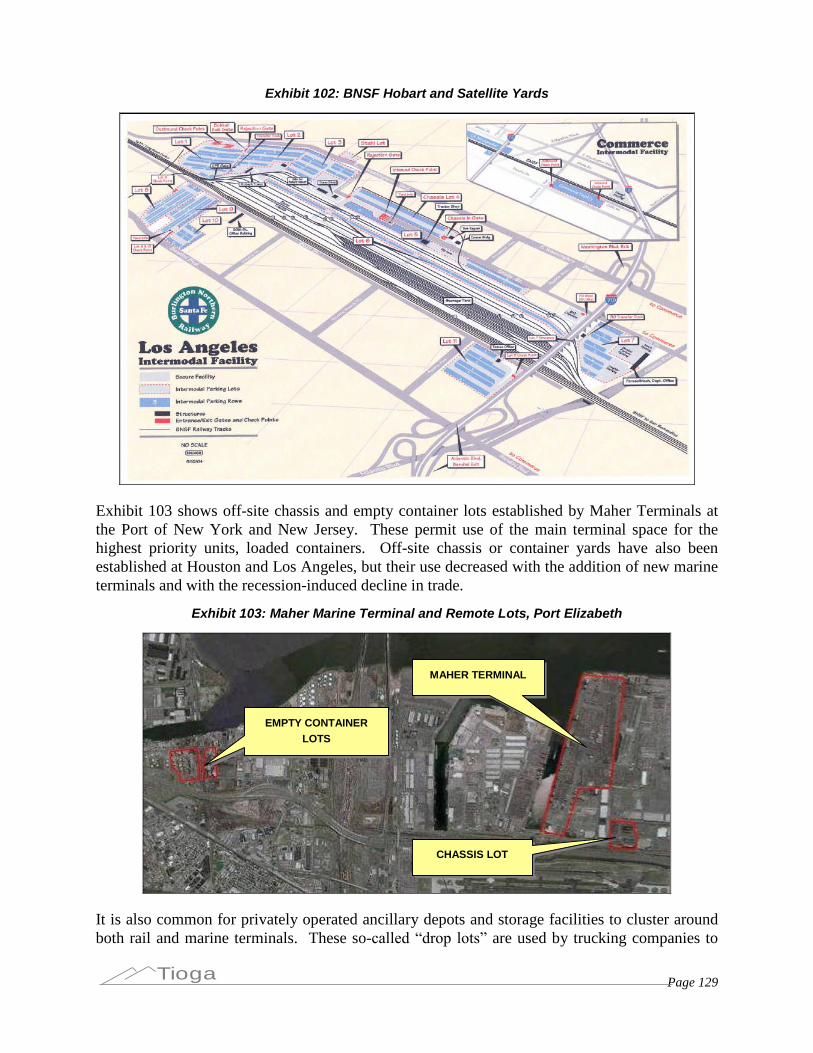
Page 129Tioga
Exhibit 102: BNSF Hobart and Satellite Yards
Exhibit 103 shows off-site chassis and empty container lots established by Maher Terminals atthe Port of New York and New Jersey. These permit use of the main terminal space for thehighest priority units, loaded containers. Off-site chassis or container yards have also beenestablished at Houston and Los Angeles, but their use decreased with the addition of new marineterminals and with the recession-induced decline in trade.
Exhibit 103: Maher Marine Terminal and Remote Lots, Port Elizabeth
It is also common for privately operated ancillary depots and storage facilities to cluster aroundboth rail and marine terminals. These so-called “drop lots” are used by trucking companies to
EMPTY CONTAINERLOTS
CHASSIS LOT
MAHER TERMINAL
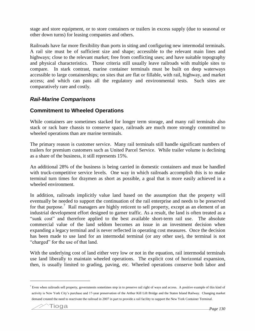
Page 130Tioga
stage and store equipment, or to store containers or trailers in excess supply (due to seasonal orother down turns) for leasing companies and others.
Railroads have far more flexibility than ports in siting and configuring new intermodal terminals.A rail site must be of sufficient size and shape; accessible to the relevant main lines andhighways; close to the relevant market; free from conflicting uses; and have suitable topographyand physical characteristics. Those criteria still usually leave railroads with multiple sites tocompare. In stark contrast, marine container terminals must be built on deep waterwaysaccessible to large containerships; on sites that are flat or fillable, with rail, highway, and marketaccess; and which can pass all the regulatory and environmental tests. Such sites arecomparatively rare and costly.
Rail-Marine Comparisons
Commitment to Wheeled Operations
While containers are sometimes stacked for longer term storage, and many rail terminals alsostack or rack bare chassis to conserve space, railroads are much more strongly committed towheeled operations than are marine terminals.
The primary reason is customer service. Many rail terminals still handle significant numbers oftrailers for premium customers such as United Parcel Service. While trailer volume is decliningas a share of the business, it still represents 15%.
An additional 28% of the business is being carried in domestic containers and must be handledwith truck-competitive service levels. One way in which railroads accomplish this is to maketerminal turn times for draymen as short as possible, a goal that is more easily achieved in awheeled environment.
In addition, railroads implicitly value land based on the assumption that the property willeventually be needed to support the continuation of the rail enterprise and needs to be preservedfor that purpose.7 Rail managers are highly reticent to sell property, except as an element of anindustrial development effort designed to garner traffic. As a result, the land is often treated as a“sunk cost” and therefore applied to the best available short-term rail use. The absolutecommercial value of the land seldom becomes an issue in an investment decision whenexpanding a legacy terminal and is never reflected in operating cost measures. Once the decisionhas been made to use land for an intermodal terminal (or any other use), the terminal is not“charged” for the use of that land.
With the underlying cost of land either very low or not in the equation, rail intermodal terminalsuse land liberally to maintain wheeled operations. The explicit cost of horizontal expansion,then, is usually limited to grading, paving, etc. Wheeled operations conserve both labor and
7 Even when railroads sell property, governments sometimes step in to preserve rail right of ways and access. A positive example of this kind of
activity is New York City’s purchase and 17-year preservation of the Arthur Kill Lift Bridge and the Staten Island Railway. Changing market
demand created the need to reactivate the railroad in 2007 in part to provide a rail facility to support the New York Container Terminal.
Page 131Tioga
capital, which are critical aspects of the railroads’ calculations. Rail intermodal terminals thususe land as a low-cost resource. The underlying value of the land is usually considered onlywhen the railroad is faced with a choice between using a large parcel for continuing intermodaloperations or selling it on the open market. Such measures are fairly uncommon, and are usuallytaken only when the buyer provides a practical alternative that permits the continuation of thebusiness.
Chassis Supply
A railroad’s intermodal business can be categorized by its equipment type, e.g., trailers,international containers, or domestic containers. Chassis are required for the latter twocategories. For the international business, railroads require the lines to provide a chassis to theterminal at the time of unloading. Some railroads may require the lines to remove themimmediately after the train has been loaded.
Steamship lines often transfer this responsibility to a pool operator who is typically providedwith on-site space to store chassis. There are three providers of pool chassis: Ocean CarriersEquipment Management Association (OCEMA), Seacastle (Trac), and Flexivan. Each of theseorganizations is now developing large regional pools with multiple termination points on bothrail and marine terminals. OCEMA pools are cooperative organizations to which lines contributechassis they own, and which OCEMA manages through its Consolidated Chassis Managementsubsidiary. These pools are growing both in numbers of chassis and geographical scope.
Flexibility
Rail terminal operators have far more flexibility than marine terminal operators in adjusting bothnear-term and long-term capacity.
Rail terminal operators can vary the size of the workforce in much finer movements. The railworkforce, regardless of union representation, does not have a minimum gang size orsupervisory requirements comparable to Longshore unions. Rail terminal managers also havemore flexibility in assigning workers to different tasks and in scheduling shifts and breaks. Railterminal contractors who have worked with different unions have commented that the differencesin work rules are much more important than the differences in wage rates.
Rail terminal operators also have more flexibility in the types and numbers of lift machines andother equipment used. Marine container cranes are multi-million dollar investments with longlead times. They are rarely moved between terminals until retired or replaced. In contrast, theequipment used at rail terminals is basically the same as that used in the container yards ofmarine terminals: rubber-tired gantries, side loaders, reach stackers, empty handlers, and yardtractors. These units can be shifted between terminals as demand changes (although the cost ofdismantling and moving a gantry crane is significant).
At a marine terminal, the ultimate constraints on capacity are the length and depth of the berthand the area available for the container yard. Within these overall constraints, the throughputcapacity and efficiency of the terminal are matters of capital investment, technology, andmanagement. The corresponding features of a rail intermodal terminal are the number andlength of loading and storage tracks and the area available for parking. A critical distinction is
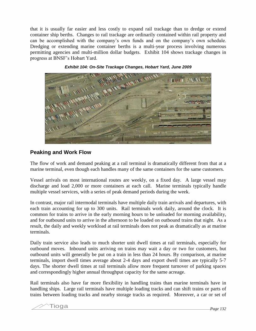
Page 132Tioga
that it is usually far easier and less costly to expand rail trackage than to dredge or extendcontainer ship berths. Changes to rail trackage are ordinarily contained within rail property andcan be accomplished with the company’s own funds and on the company’s own schedule. Dredging or extending marine container berths is a multi-year process involving numerouspermitting agencies and multi-million dollar budgets. Exhibit 104 shows trackage changes inprogress at BNSF’s Hobart Yard.
Exhibit 104: On-Site Trackage Changes, Hobart Yard, June 2009
Peaking and Work Flow
The flow of work and demand peaking at a rail terminal is dramatically different from that at amarine terminal, even though each handles many of the same containers for the same customers.
Vessel arrivals on most international routes are weekly, on a fixed day. A large vessel maydischarge and load 2,000 or more containers at each call. Marine terminals typically handlemultiple vessel services, with a series of peak demand periods during the week.
In contrast, major rail intermodal terminals have multiple daily train arrivals and departures, witheach train accounting for up to 300 units. Rail terminals work daily, around the clock. It iscommon for trains to arrive in the early morning hours to be unloaded for morning availability,and for outbound units to arrive in the afternoon to be loaded on outbound trains that night. As aresult, the daily and weekly workload at rail terminals does not peak as dramatically as at marineterminals.
Daily train service also leads to much shorter unit dwell times at rail terminals, especially foroutbound moves. Inbound units arriving on trains may wait a day or two for customers, butoutbound units will generally be put on a train in less than 24 hours. By comparison, at marineterminals, import dwell times average about 2-4 days and export dwell times are typically 5-7days. The shorter dwell times at rail terminals allow more frequent turnover of parking spacesand correspondingly higher annual throughput capacity for the same acreage.
Rail terminals also have far more flexibility in handling trains than marine terminals have inhandling ships. Large rail terminals have multiple loading tracks and can shift trains or parts oftrains between loading tracks and nearby storage tracks as required. Moreover, a car or set of
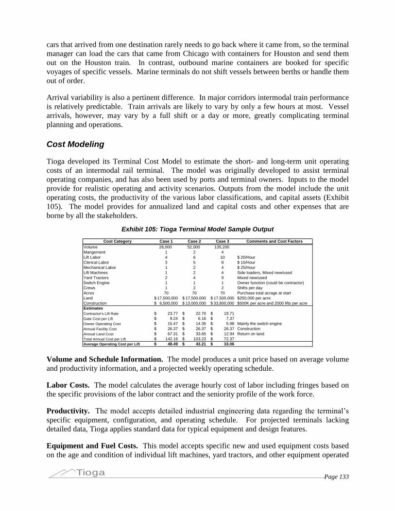
Page 133Tioga
cars that arrived from one destination rarely needs to go back where it came from, so the terminalmanager can load the cars that came from Chicago with containers for Houston and send themout on the Houston train. In contrast, outbound marine containers are booked for specificvoyages of specific vessels. Marine terminals do not shift vessels between berths or handle themout of order.
Arrival variability is also a pertinent difference. In major corridors intermodal train performanceis relatively predictable. Train arrivals are likely to vary by only a few hours at most. Vesselarrivals, however, may vary by a full shift or a day or more, greatly complicating terminalplanning and operations.
Cost Modeling
Tioga developed its Terminal Cost Model to estimate the short- and long-term unit operatingcosts of an intermodal rail terminal. The model was originally developed to assist terminaloperating companies, and has also been used by ports and terminal owners. Inputs to the modelprovide for realistic operating and activity scenarios. Outputs from the model include the unitoperating costs, the productivity of the various labor classifications, and capital assets (Exhibit105). The model provides for annualized land and capital costs and other expenses that areborne by all the stakeholders.
Exhibit 105: Tioga Terminal Model Sample Output
Cost Category Case 1 Case 2 Case 3 Comments and Cost FactorsVolume 26,000 52,000 135,200Mangement 1 2 4Lift Labor 4 6 10 $ 20/HourClerical Labor 3 5 8 $ 15/HourMechanical Labor 1 2 4 $ 25/HourLift Machines 1 2 4 Side loaders, Mixed new/usedYard Tractors 2 4 9 Mixed new/usedSwitch Engine 1 1 1 Owner function (could be contractor)Crews 1 2 2 Shifts per dayAcres 70 70 70 Purchase total acrage at startLand 17,500,000$ 17,500,000$ 17,500,000$ $250,000 per acreConstruction 6,500,000$ 13,000,000$ 33,800,000$ $500K per acre and 2000 lifts per acreEstimatesContractor's Lift Rate 23.77$ 22.70$ 19.71$Gate Cost per Lift 9.24$ 6.16$ 7.37$Owner Operating Cost 15.47$ 14.35$ 5.98$ Mainly the switch engineAnnual Facility Cost 26.37$ 26.37$ 26.37$ ConstructionAnnual Land Cost 67.31$ 33.65$ 12.94$ Return on landTotal Annual Cost per Lift 142.16$ 103.23$ 72.37$Average Operating Cost per Lift 48.49$ 43.21$ 33.06$
Volume and Schedule Information. The model produces a unit price based on average volumeand productivity information, and a projected weekly operating schedule.
Labor Costs. The model calculates the average hourly cost of labor including fringes based onthe specific provisions of the labor contract and the seniority profile of the work force.
Productivity. The model accepts detailed industrial engineering data regarding the terminal’s specific equipment, configuration, and operating schedule. For projected terminals lackingdetailed data, Tioga applies standard data for typical equipment and design features.
Equipment and Fuel Costs. This model accepts specific new and used equipment costs basedon the age and condition of individual lift machines, yard tractors, and other equipment operated
Page 134Tioga
by the terminal contractor. Maintenance costs are calculated based on typical preventivemaintenance practices and labor costs as described above. Fuel costs are calculated based onlocal fuel cost and specific equipment usage rates.
Other Operating Costs. Other operating costs such as utilities, security, ordinary terminalmaintenance, terminal operator’s profit, etc., are included based on typical industry operating practices.
Capital Costs. Tioga’smodel expresses land, facility, and other large capital costs as unit costsbased on expected life volumes and interest rates.
Outputs from the model include the cost per unit of the terminal operation, the productivity ofthe various labor crafts, and capital assets. Unit costs can be displayed for any required costelement. As an in-kind contribution, Tioga offered to use the intermodal terminal productivityand cost model to analyze potential productivity measures and their applicability to marinecontainer terminals.
Scenarios
Tioga developed six hypothetical scenarios based on a notional 50-acre rail intermodal terminalwith differing operating assumptions, each of which is applicable to rail and marine terminaldevelopment. The scenarios are designed to illustrate the impact of the value of land on arailroad’s terminal development strategy.
Scenario 1. This scenario represents the situation faced by a new terminal developer in theMidwest during the current recession. Land is plentiful and free. A developer will provide theland to a prospective intermodal terminal for free in the expectation that landing this “anchor tenant” will enhance the value of nearby properties. The basic assumption is that land is free andthe terminal will operate at 2,000 lifts per acre, 100,000 lifts annually. This is a common,medium-sized intermodal facility. Yard labor productivity is estimated at 4.29 lifts per man-hour, which is relatively high, and the capital cost allocation for terminal equipment ownership isestimated at $3.28 per lift.
The Tioga model estimated the expected full price per lift for this terminal at approximately $60per lift. This includes all the operating costs, equipment cost, and facility costs. Capital costsare annualized assuming standard finance lives and salvage values. Operating costs include railswitch crews, facility costs, terminal operator costs, and terminal owner costs. A breakdown bycost category is included in Table 1 below.
Scenario 2. This scenario is identical to Scenario 1 except that land costs are more typical,$100,000 per acre. This adds $4 per lift to the previous scenario.
Scenario 3. This scenario is the same as Scenario 1 and 2 except that land is assumed to bemuch more expensive at $1,000,000 per acre. This makes the full cost of the terminal $100 perlift. This scenario is unrealistic in that management actions would be taken to preclude this kindof operation. Most likely the land would be sold at a profit, and, if warranted, a new, less costlylocation for the intermodal terminal would be sought.
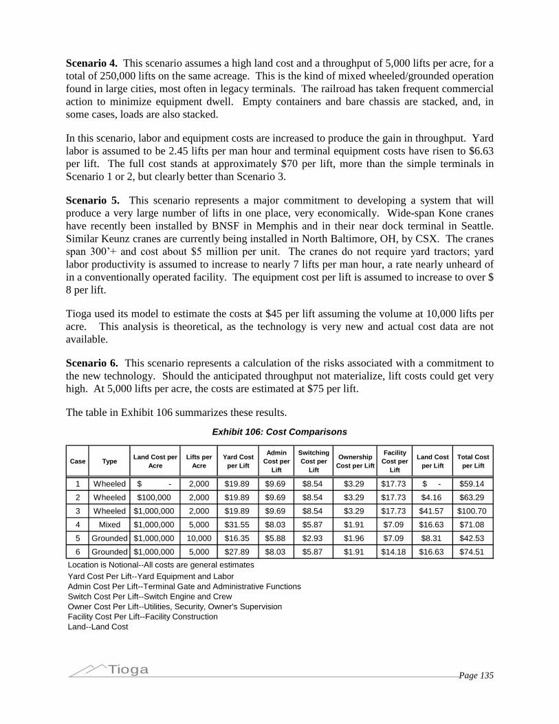
Page 135Tioga
Scenario 4. This scenario assumes a high land cost and a throughput of 5,000 lifts per acre, for atotal of 250,000 lifts on the same acreage. This is the kind of mixed wheeled/grounded operationfound in large cities, most often in legacy terminals. The railroad has taken frequent commercialaction to minimize equipment dwell. Empty containers and bare chassis are stacked, and, insome cases, loads are also stacked.
In this scenario, labor and equipment costs are increased to produce the gain in throughput. Yardlabor is assumed to be 2.45 lifts per man hour and terminal equipment costs have risen to $6.63per lift. The full cost stands at approximately $70 per lift, more than the simple terminals inScenario 1 or 2, but clearly better than Scenario 3.
Scenario 5. This scenario represents a major commitment to developing a system that willproduce a very large number of lifts in one place, very economically. Wide-span Kone craneshave recently been installed by BNSF in Memphis and in their near dock terminal in Seattle.Similar Keunz cranes are currently being installed in North Baltimore, OH, by CSX. The cranesspan 300’+ and cost about $5 million per unit. The cranes do not require yard tractors; yard labor productivity is assumed to increase to nearly 7 lifts per man hour, a rate nearly unheard ofin a conventionally operated facility. The equipment cost per lift is assumed to increase to over $8 per lift.
Tioga used its model to estimate the costs at $45 per lift assuming the volume at 10,000 lifts peracre. This analysis is theoretical, as the technology is very new and actual cost data are notavailable.
Scenario 6. This scenario represents a calculation of the risks associated with a commitment tothe new technology. Should the anticipated throughput not materialize, lift costs could get veryhigh. At 5,000 lifts per acre, the costs are estimated at $75 per lift.
The table in Exhibit 106 summarizes these results.
Exhibit 106: Cost Comparisons
Case TypeLand Cost per
AcreLifts per
AcreYard Cost
per Lift
AdminCost per
Lift
SwitchingCost per
Lift
OwnershipCost per Lift
FacilityCost per
Lift
Land Costper Lift
Total Costper Lift
1 Wheeled $ - 2,000 $19.89 $9.69 $8.54 $3.29 $17.73 $ - $59.14
2 Wheeled $100,000 2,000 $19.89 $9.69 $8.54 $3.29 $17.73 $4.16 $63.29
3 Wheeled $1,000,000 2,000 $19.89 $9.69 $8.54 $3.29 $17.73 $41.57 $100.70
4 Mixed $1,000,000 5,000 $31.55 $8.03 $5.87 $1.91 $7.09 $16.63 $71.08
5 Grounded $1,000,000 10,000 $16.35 $5.88 $2.93 $1.96 $7.09 $8.31 $42.53
6 Grounded $1,000,000 5,000 $27.89 $8.03 $5.87 $1.91 $14.18 $16.63 $74.51
Owner Cost Per Lift--Utilities, Security, Owner's SupervisionFacility Cost Per Lift--Facility ConstructionLand--Land Cost
Location is Notional--All costs are general estimatesYard Cost Per Lift--Yard Equipment and LaborAdmin Cost Per Lift--Terminal Gate and Administrative FunctionsSwitch Cost Per Lift--Switch Engine and Crew
Page 136Tioga
As the case study shows, land costs represent about $4 or less per lift at a typical wheeledintermodal terminal, less than 10% of the fully allocated cost per lift. When land costs increase,this cost grows proportionally until costly land saving strategies are instituted. These strategiesresult in an increase in the cost per lift as throughput per acre grows, but the cost increase is lessthan the cost of expansion property.
Scenario 5 shows that CSX and BNSF’s new wide crane technology holds some promise for lowcost terminal handling, but only if a very high volume is maintained and most likely only in afully stacked environment.