Improving Forecasts of State Failure - Gary King - Harvard University

World Politics 53.4, July 2001

Improving Forecasts of State Failure

Gary King Langche Zeng

Abstract

This article offers the first independent scholarly evaluation of the claims, forecasts,

and causal inferences of the State Failure Task Force and its efforts to forecast when

states will fail. State failure refers to the collapse of the authority of the central

government to impose order, as in civil wars, revolutionary wars, genocides,

politicides, and adverse or disruptive regime transitions. States that sponsor terrorism

or allow it to be organized within their borders are all failed states. This task force,

set up at the behest of Vice President Gore in 1994, has been led by a group of

distinguished academics working as consultants to the U.S. CIA. State Failure Task

Force reports and publications have received attention in the media, in academia, and

from public decision makers. The article identifies several methodological errors in

the task force work that cause its reported forecast probabilities of conflict to be too

large, its causal inferences to be biased in unpredictable directions, and its claims of

forecasting performance to be exaggerated. However, the article also finds that the

task force has amassed the best and most carefully collected data on state failure to

date, and the required corrections provided in this article, although very large in

effect, are easy to implement. The article also demonstrates how to improve

forecasting performance to levels significantly greater than even corrected versions

of its models. Although the matter is still a highly uncertain endeavor, the authors are

nevertheless able to offer the first accurate forecasts of state failure, along with

procedures and results that may be of practical use in informing foreign policy

decision making. The article also describes a number of strong empirical regularities

that may help in ascertaining the causes of state failure.

Subject Headings:

International relations -- Risk assessment.

International relations -- Forecasting.

State, The.

World Politics 53 ( July 2001), 623–58

Research Note

IMPROVING FORECASTS OF STATE FAILURE

By GARY KING and LANGCHE ZENG*

I. INTRODUCTION

STATE failure” refers to the complete or partial collapse of state au-thority, such as occurred in Somalia and Bosnia. Failed states have

governments with little political authority or ability to impose the ruleof law. They are usually associated with widespread crime, violent con-flict, or severe humanitarian crises, and they may threaten the stabilityof neighboring countries. States that sponsor international terrorism orallow it to be organized from within their borders are all failed states.Since the consequences for the citizens of these states can be very se-vere and the costs to the international community of rebuilding thestates are often substantial, there has long been considerable interest indeveloping methods of risk assessment and early warning systems inthe hope that foreign aid could be directed to prevent states from fail-ing. In 1994, with these goals in mind, the U.S. government, at the be-hest of Vice President Gore, established and funded the State FailureTask Force, a panel of distinguished academic social scientists, expertsin data collection, and consultants in statistical methods. Although the

* The authors have no formal or informal relationship with the State Failure Task Force or the taskforce’s sponsor, the U.S. Central Intelligence Agency. We thank Matt Baum for research assistance;Jim Alt, Aslaug Asgeirsdottir, Bob Bates, Ben Bishin, Lee Epstein, Jim Fearon, Charles Franklin,Jeff Frieden, Kristian Gleditsch, Jack Goldstone, David Laitin, Chris Murray, Kevin Quinn, KenScheve, Alan Stain, Ben Valentino, Jonathan Wand, and Mark Woodward for helpful discussions; theState Failure Task Force for collective written comments; Bob Bates for his suggestion that we take onthis project; and the National Science Foundation (SBR-9729884, SBR-9753126, and IIS-9874747),the National Institutes of Aging, and the World Health Organization for research support. For pro-viding us copy of the task force data, we thank task force members Bob Bates and Monte Marshall. Alldata referenced in this article are available at http://gking.harvard.edu, and for making this pos sible weare thankful for the guidance and assistance of Dick Cooper and the efforts of attorneys Kim Budd,Bob Donin, Allan Ryan, and Bob Iulioano in the Harvard University General Council's office.

“

v53.i4.623.king 9/27/01 5:25 PM Page 623

Aileen

task force does not use classified information, the data amassed arenonetheless impressive: more than a thousand variables, each carefullycollected and documented and many with value added beyond what isavailable from other sources. (See Appendix 1.) The task force, still inoperation, has produced over two hundred pages of widely distributedformal reports and analyses1 and several published article-length sum-maries.2 This work has received attention in the popular news media3

and “has gained substantial visibility and credibility among those re-sponsible for the analysis of global security and for planning U.S. for-eign policy,”4 an uncommon achievement for quantitative analyses inthis field.

The task force reports were aimed at policymakers, but the researchhas been of considerable interest to the scholarly community as well.The authors make stunning claims about their success at forecastingthese highly heterogeneous and idiosyncratic events, and they draw nu-merous important inferences about the causes of a critical and under-studied political phenomenon. In this article we provide the firstindependent scholarly evaluation of the methods, analyses, and claimsof the State Failure Task Force. We first identify and correct severalmethodological errors and then show how to use the task force’s datato improve forecasts of state failure substantially beyond even appropri-ately corrected versions of its statistical models. We hope that this arti-cle can then help to connect the goals and efforts of the policy andacademic communities in understanding and perhaps even addressingthis critical global problem. The work analyzed here also touches on anunusually wide range of underutilized methods and relevant method-ological issues; we seek to clarify some of these so that scholars can usethem more productively.

624 WORLD POLITICS

1 Daniel C. Esty, Jack Goldstone, Ted Robert Gurr, Pamela T. Surko, and Alan N. Unger, WorkingPapers: State Failure Task Force Report (McLean, Va.: Science Applications International Corporation,1995); Daniel C. Esty, Jack Goldstone, Ted Robert Gurr, Barbara Harff, Pamela T. Surko, Alan N.Unger, and Robert S. Chen, The State Failure Task Force Report: Phase II Findings (McLean, Va.: Sci-ence Applications International Corporation, 1998).

2 Daniel C. Esty, Jack Goldstone, Ted Robert Gurr, Barbara Harff, Pamela T. Surko, Alan N. Unger,and Robert S. Chen, “The State Failure Project: Early Warning Research for U .S. Foreign PolicyPlanning,” in John L. Davies and Ted Robert Gurr, eds., Preventive Measures: Building Risk Assessmentand Crisis Early Warning Systems (Lanham, Md.: Rowman and Littlefield, 1998); Daniel C. Esty, JackGoldstone, Ted Robert Gurr, Barbara Harff, Marc Levy, Geoffrey D. Dabelko, Pamela T. Surko, andAlan N. Unger, “The State Failure Report: Phase II Findings,” Environmental Change and SecurityProject Report 5 (Summer 1999).

3 For example, Tim Zimmermann, “CIA Study: Why Do Countries Fall Apart? Al Gore Wanted toKnow,” U.S. News and World Report, March 12, 1996.

4 Esty et al. (fn. 2, 1998), 27–38; and, e.g., John C. Gannon, The Global Infectious Disease Threat andIts Implications for the United States (U.S. National Intelligence Council, http://www.cia.gov/cia/publications/nie/report/nie99-17d.html, 2000).

v53.i4.623.king 9/27/01 5:25 PM Page 624

II. TASK FORCE DATA AND MODELS

According to the task force, a “state failure” consists of revolutionarywars (“sustained military conflicts between insurgents and central gov-ernments, aimed at displacing the regime”), genocides and politicides(“sustained policies by states or their agents and, in civil wars, by con-tending authorities that result in the deaths of a substantial portion ofmembers of communal or political groups”), and adverse or disruptiveregime transitions (“major, abrupt shifts in patterns of governance, in-cluding state collapse, periods of severe regime instability, and shifts to-ward authoritarian rule).”5 The authors intentionally included fairlydiverse events in their definition of state failure in order to follow theguidelines of policymakers as articulated to the task force. This may bea reasonable starting point, in part, because it increases the number ofevents in the data set, but also because it assumes that the benefits ofhaving more events outweigh the costs of lower predictive ability andmodel incoherence resulting from increased heterogeneity in the out-come variable. In this article we use the dependent variable as concep-tualized and measured by the task force (in order to isolate the effectsof our methodological corrections), but in all likelihood a differentcausal structure underlies each component of the constructed conceptof “state failure.” Although our very flexible model will pick up some ofthese differences, we recommend that future researchers experimentwith fitting different models to each component. We return to thisissue in the conclusion.

According to the definition used by the task force, 127 state failureshad commenced between 1955 and 1998 in some of 195 distinct coun-tries in the data set.6 Thus, the outcome variable is state failure, whichwe denote as Yi , coded 1 for country-years in which a state failurestarted and 0 for country-years with no failure. Since the goal of thetask force was to explain the onset of state failure (incidence rather thanprevalence, in epidemiological terms), subsequent years in which acountry remained in a state of failure are dropped.

The task force collected its data via a case-control design, which isespecially efficient for rare events data.7 First, it collects all cases of fail-

FORECASTS OF STATE FAILURE 625

5 Esty et al. (fn. 2, 1998), 27–38.6 Fewer than 195 countries appear in the data set in any one year. For example, Germany, East Ger-

many, and West Germany are three separate items in this count, even though for any one year in thedata set, either Germany or East and West Germany appear. Countries enter the data set in 1955 orwhen they first came into existence if later; countries remain in the data set after an episode of failure.In addition, the task force was required by the U.S. government to omit the United States from allanalyses. They also omitted countries with fewer than half a million people.

7 Norman E. Breslow, “Statistics in Epidemiology: The Case-Control Study,” Journal of the American

v53.i4.623.king 9/27/01 5:25 PM Page 625

ure. Then for each failure it randomly draws three nonfailures from thesame year. The advantage of this scheme is clear in comparison with arandom sample, which could by chance miss many important events.The 1:3 ratio is not required for case-control studies, although all casesof failure were used and every additional control adds progressively lessinformation after the first, so there is little point of continuing muchfurther if data collection is expensive. The task force then coded hun-dreds of explanatory variables.8

To choose a model, the task force authors lagged all the explanatoryvariables by two years so that their models would predict two years intothe future. They then conducted an extensive search process fittingtheir entire data set via logistic regression numerous times to differentspecifications (that is, sets of explanatory variables). They used geneticalgorithms, stepwise logistic regression, and other informal proceduresto examine other specifications. Listwise deletion was applied to eachspecification by deleting a country-year if any variable in the model wasmissing (so that each logit model was run on a different set of country-years). They also report performing a first cut, narrowing the list ofvariables to thirty-one on the basis of univariate t or chi-square tests.Then “combinations of two, three, five, and up to 14 variables con-tained in the 31-variable set were examined together in an inductiveapproach to specifying the most accurate analysis or model.”9 Even thissecond step was constrained by the qualitative knowledge of theauthors, as well as by some external rules, since the number of combi-nations of explanatory variables that could have been tested in this wayis over 773 million (if each combination took 10 seconds to run andevaluate, it would take 245 years to complete them all). The summarymeasure they used to judge the quality of each model was not identified.

This process led the task force to choose a simple logistic regressionmodel with three variables: democracy (the standard Polity III democ-racy and autocracy scores, collapsed into the categories of full democ-racy, partial democracy, and autocracy and coded as two dummyvariables), trade openness (the log of imports plus exports as a percentageof GDP), and infant mortality (the log of the ratio of the infant mortal-ity rate to the world median). (This entire process was repeated using

626 WORLD POLITICS

Statistical Association 91 (March 1996); Gary King and Langche Zeng, “Explaining Rare Events in In-ternational Relations,” International Organization (forthcoming), preprint at http://gking.harvard.edu.

8 We focus only on the task force’s so-called “global model.” Its data set includes 1,231 variables, al-though many of these are recodes of other variables or markers of problems with individual observa-tions. Although the task force writings indicate that it used only the case-control data, its data setcontains at least some information and always Yi, for every country.

9 Esty et al. (fn. 2, 1998).

v53.i4.623.king 9/27/01 5:25 PM Page 626

“neural network clustering,” the specific version of which the authorsdo not identify, although they conclude that it does no better than theirlogit model.)

There is much to criticize in this relatively atheoretical search pro-cedure, but without a theory that rules out hundreds of the variables inthe task force data set, uniformly superior statistical procedures do notyet exist (although see West et al.)10 The task force’s ultimate modelchoice was parsimonious and (aside from the case-control corrections,which had enormous effects) was not easy to surpass.

Since the analyses conducted by the task force and used by policy-makers are based on continuously updated data, variables, and meth-ods, we requested and received the data and results from their currentmodel of choice, which still includes the same three variables. In allother ways, too, differences between the data used in their publishedreport and those used in the newer version were minor and always in-consequential for the points discussed herein. Except where noted, webase all our analyses and comparisons on these new data. In the final taskforce model, 108 failures and 315 nonfailures were included, and 85 otherobservations were dropped due to the application of listwise deletion.

III. CORRECTING METHODOLOGICAL ERRORS

In this section we discuss methodological errors and opportunities forimproving on the State Failure Task Force statistical analyses. Weconsider problems stemming from (1) their case-control design, (2) theway they evaluate forecasting performance, (3) the way they distinguishin-sample fit from out-of-sample forecasts, and (4) the way they treatmissing data.

CASE-CONTROL PROBLEMS

The task force collects data by selecting on the dependent variable, aprocedure known to cause bias.11 As the task force makes no correctionfor this problem, all its estimates are therefore biased, in most casesquite severely.

Most obviously, the marginal distribution of Y is biased in case-control sampling. In the present case, the fraction of state failures in the


10 Mike West, Joseph R. Nevins, Jeffrey R. Marks, Rainer Spang, and Harry Zuzuan, “Bayesian Re-gression Analysis in the ‘Large p, Small n’ Paradigm with Application in DNA Microarray Studies”(Manuscript, Duke University, 2000).

11 For example, Gary King, Robert O. Keohane, and Sidney Verba, Designing Social Inquiry: Scien-tific Inference in Qualitative Research (Princeton: Princeton University Press, 1994).

v53.i4.623.king 9/27/01 5:25 PM 27

data, y–, is y– = 0.255, whereas the fraction of failures in the universe ofcountry-years, which we denote τ, is only τ = 0.0168.

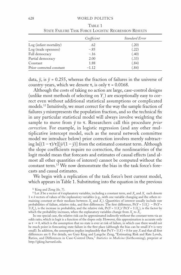
Although the costs of taking no action are large, case-control designs(unlike most methods of selecting on Yi ) are exceptionally easy to cor-rect even without additional statistical assumptions or complicatedmodels.12 Intuitively, we must correct for the way the sample fraction offailures y misrepresents the population fraction, and so the technical fixin any particular statistical model will always involve weighting thesample to move from y– to τ. Researchers call this procedure priorcorrection. For example, in logistic regression (and any other mul-tiplicative intercept model, such as the neural network committeemodel we introduce below) prior correction involves merely subtract-ing ln[(1 – τ)/τ][y–/(1 – y–)] from the estimated constant term. Althoughthe slope coefficients require no correction, the nonlinearities of thelogit model mean that forecasts and estimates of causal effects (and al-most all other quantities of interest) cannot be computed without theconstant term.13 We now demonstrate the bias in the task force’s fore-casts and causal estimates.

We begin with a replication of the task force’s best current model,which appears in Table 1. Substituting into the equation in the previous

628 WORLD POLITICS

12 King and Zeng (fn. 7).13 Let X be a vector of k explanatory variables, including a constant term, and X0 and X1 each denote

1 × k vectors of values of the explanatory variables (e.g., with one variable changing and the others re-maining constant at their medians between X0 and X1). Quantities of interest usually include rawprobabilities of failure, relative risks, and first differences. The first difference, Pr(Y = 1|X1) – Pr(Y =1|X0 ), is the increase in probability, and the relative risk, Pr(Y = 1|X1)/ Pr(Y = 1|X0 ), is the factor bywhich the probability increases, when the explanatory variables change from X0 to X1.

In one special case, the relative risk can be approximated indirectly without the constant term via anodds ratio, which in logit is a function of the slopes only. However, this approximation is accurate onlyas τ → 0, which is the assumption that no state is ever at risk of failure, in which case there would notbe much point in forecasting state failure in the first place (although the bias can be small if τ is verysmall). In addition, the assumption implies implausibly that Pr(Y = 1|X ) = 0 for any X and that all firstdifferences are 0. For details, see Gary King and Langche Zeng, “Estimating Risk and Rate Levels,Ratios, and Differences in Case-Control Data,” Statistics in Medicine (forthcoming), preprint athttp://gking.harvard.edu.

TABLE 1STATE FAILURE TASK FORCE LOGISTIC REGRESSION RESULTS

Coefficient Standard Error

Log (infant mortality) .62 (.20)Log (trade openness) –.85 (.22)Full democracy –.16 (.40)Partial democracy 2.00 (.33)Constant 1.88 (.84)Prior-corrected constant –1.12 (.84)

v53.i4.623.king 9/27/01 5:25 PM Page 628

paragraph, we calculate that the correction factor in this case is 3.0. Wethus subtract 3.0 from the logit constant to produce the prior-correctedconstant in the last line. (This may seem like a small number, but as weshall see, it has a large effect on the quantities of interest.)

BIAS IN TASK FORCE FORECASTS

Although the task force repeatedly refers to its forecast numbers as“probabilities,” they are not probabilities since they were not prior cor-rected. For an example of the bias in the numbers produced by the taskforce, consider the simple case with no explanatory variables (or nonewith an effect). In this situation a predicted probability of failure, basedon the global population of country-years or the corrected case-controlsample, would equal 0.0168. However, the uncorrected case-controlsample yields an estimate fifteen times larger, an incredible predictionthat slightly more than a quarter of the states in the world will fail inany one year. When the task force includes explanatory variables, someof the probabilities extend to 0.89, which is implausibly large for thisproblem.

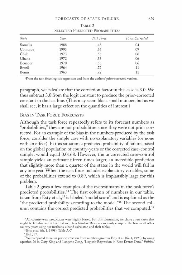
Table 2 gives a few examples of the overestimates in the task force’spredicted probabilities.14 The first column of numbers in our table,taken from Esty et al.,15 is labeled “model score” and is explained as the“the predicted probability according to the model.”16 The second col-umn contains the correct predicted probabilities that we computed.17


14 All country-year predictions were highly biased. For this illustration, we chose a few cases thatmight be familiar and a few that were less familiar. Readers can easily compute the bias in all othercountry-years using our methods, a hand calculator, and their tables.

15 Esty et al. (fn. 1, 1998), Table A-7.l6 Ibid., 57.17 We computed these via prior correction from numbers given in Esty et al. (fn. 1, 1998), by using

equation 26 in Gary King and Langche Zeng, “Logistic Regression in Rare Events Data,” Political

TABLE 2SELECTED PREDICTED PROBABILITIESa

State Year Task Force Prior Corrected

Somalia 1988 .45 .04Comoros 1995 .66 .09Chile 1973 .56 .06Ghana 1972 .55 .06Ecuador 1970 .58 .06Brazil 1964 .72 .11Benin 1963 .72 .11

aFrom the task force logistic regression and from the authors’ prior-corrected version.

v53.i4.623.king 9/27/01 5:25 PM Page 629

By any substantive or statistical measure, the task force estimates are farfrom accurate and range from 6.54 to 11.25 times too large. The taskforce authors included several long tables in their reports with numer-ous estimated probabilities, but unfortunately the lack of prior correc-tion means that every such estimate is incorrect, sometimes by moreand sometimes by less than the examples in Table 2. Fortunately, theseare easy to correct.

BIAS IN TASK FORCE CAUSAL INFERENCES

We demonstrate the bias in the causal effects estimated from the un-corrected case-control analysis with one key example, highly touted bythe task force in all its writings: the effect of democracy on the proba-bility of state failure. Table 3 gives relative risks and first differences(with 95 percent confidence intervals) computed from the original un-corrected model and with appropriate corrections. For example, when anation moves from autocratic to partial democracy and other variablesare held constant at their global medians, the task force’s biased esti-mate is that the probability of state failure more than triples (increasesby 3.66). However, the correct estimate (7.04) is nearly twice as large. Asimilar bias, of about a factor of two (4.14 to 8.08), occurs when mov-ing from full to partial democracy.

Unfortunately, the bias correction does not always increase the sizeof estimated effects as it happens to with these selected relative risks.

630 WORLD POLITICS

Analysis (forthcoming), preprint at http://gking.harvard.edu. Since the raw data are not needed for thiscalculation, we stuck to the published version, which was based on a data set that differed slightly fromthe updated one we used. We also reproduce this with the new data, and there were only very minordifferences.

TABLE 3BIASED AND CORRECTED QUANTITIES OF INTERESTa

(WITH 95% CONFIDENCE INTERVALS IN PARENTHESES)

Relative Risk First Difference

Autocracy to partial democracytask force 3.66 (2.45, 5.61) .42 (.27, .55)corrected 7.04 (3.57, 13.21) .06 (.03, .09)

Full to partial democracytask force 4.14 (2.37, 7.66) .43 (.27, .58)corrected 8.08 (3.58, 18.59) .06 (.03, .10)

aThe relative risk is the ratio and the first difference is the difference in the probability of state fail-ure when changing the democracy variables, holding other variables constant at their global medians.

v53.i4.623.king 9/27/01 5:25 PM Page 630

For example, we also computed first differences for these same causalcounterfactuals and found the bias to be in the opposite direction. Table3 shows that a change from autocracy to partial democracy is estimatedwith the task force’s methods to increase the probability of state failureby 0.42, which is an immense effect. The correction brings this down toa modest 0.06. A similar sevenfold change occurs when correcting thefirst difference for a change from full to partial democracy. (The direc-tion of bias between the relative risk and first difference results mayseem contradictory, but (a/b) and (a – b) are not constrained mathe-matically to change in the same direction as the estimates, a and b,change; the directions of the bias may also change in other examples.)

This same problem also occurs in the simpler context of comparingthe raw numbers the task report reports as probabilities, since the cor-rect probabilities are not preserved in the levels or even in the ratios ofor differences between their numbers. For example, when the explana-tory variables change from the profile of Somalia in 1988 to that ofBrazil in 1964 (both taken from the task force and Table A-7 repro-duced in our Table 2), the relative risk increases by a factor of 0.72/0.45= 1.6 according to their numbers, but a much larger 0.11/0.04 = 2.75when appropriately corrected. Similarly, the first difference indicates anincrease in the probability of 0.72 – 0.45 = 0.27 according to the taskforce but of only 0.11 – 0.04 = 0.07 when appropriately corrected.18

Task force estimates without prior correction do preserve the rank-ing of the (in-sample) probabilities, but this ranking by itself is not use-ful for any policy purpose: it indicates only which country has a higherrisk of failure, not whether any country is at high enough risk to war-rant spending money or risking troops. And, as we will see in the nextsection, the rankings are not preserved in real out-of-sample forecastprobabilities.

These results show that the causal estimates in the task force reportsare unreliable and the biases are in otherwise unexpected directions andmagnitudes. The biases in other comparisons of relative risks and firstdifferences that we calculated (not shown) vary widely. Fortunately, the


18 In our discussions with the task force, we learned that they sometimes estimated relative risks inTable 3 indirectly and approximately via an odds ratio (where prior correction is unnecessary; see fn.13), rather than directly and without prior correction, as assumed here. The indirect approach is alsobiased except when the expected population of failures becomes 0. The indirect approximation (andeven the phrase “odds ratio”) is never mentioned in the task force reports or other publications, but ifthe task force had used it for its written work, then its relative risk estimates computed from the logis-tic regression in Table 1 are more accurate than indicated in our Table 3. However, the task force esti-mates of relative risks, such as those computed from the probabilities in Table 2 and described in thetext above, would be as biased, and their estimates of probabilities and first differences would be con-siderably less accurate than we indicate.

v53.i4.623.king 9/27/01 5:25 PM Page 631

corrections we provide can easily be used in future work to generate ac-curate figures.

All quantities labeled “causal effects” in this section are calculatedbased on the assumptions that the counterfactuals necessary for makingcausal inferences are correct and that the task force’s model is appropri-ate. For the first, the task force assumes that infant mortality and tradeopenness are causally prior to the level of democracy. This means that ifwe could exogenously change the level of democracy in a country, theninfant mortality and trade openness would not change as a result, as as-sumed in Table 3. For the second, the task force assumes that if anycauses of state failure exist that are causally prior to and uncorrelatedwith democracy, then they are included in the equation; if an explana-tory variable exists that meets these conditions other than democracy,trade openness, and infant mortality, the task force model has addi-tional biases. The first assumption is implausible and unfortunately veryhard to correct. The second assumption is by definition unverifiable butis considerably more plausible given the task force’s extensive search forother predictive variables. We continue this discussion in Section VI.

EVALUATING FORECASTING SUCCESS

When appropriately corrected, the logistic regression models used bythe task force give estimates of the probability of state failure condi-tional on chosen values of the explanatory variables π̂ Pr(Y = 1|X ). Aseparate step, governed by decision theory, is required to decide on thebasis of π̂ whether the state in question will fail or not.

Let C denote the cost of mispredicting a state failure as a nonfailurerelative to the cost of mispredicting a nonfailure as a failure. Decisiontheory tells us that whatever C is, the optimal prediction (in the senseof minimizing total expected cost) is Y = 1 when π̂ > 1/(1 + C) and Y =0 otherwise.19 Hence, if the two possible mispredictions are equallycostly, then C = 1 and we would predict that a state will fail when π̂ >0.5. However, if the cost of mispredicting a state failure is, say, twice ascostly as mispredicting a nonfailure, then C = 2, and an optimal deci-sion process would predict state failure whenever π̂ > 1/3.

Only by applying decision theory in this way can we compare modeloutputs to the data and judge our success in prediction. The key, how-ever, is that the value of C must be decided independently of the dataand statistical results. The task force violated this rule and instead “di-

632 WORLD POLITICS

19 For example, B. D. Ripley, Pattern Recognition and Neural Networks (New York: Cambridge Uni-versity Press, 1996).

v53.i4.623.king 9/27/01 5:25 PM Page 632

vided errors evenly between ‘false positives’ and ‘false negatives.’” Ofcourse, the only way to “divide errors evenly” is to inspect the actual val-ues of Y and change C on that basis, which is inappropriate. This is easyto see when forecasting out of sample for genuine policy purposes, sincewe would not know the future values of Y when C was being chosen.

On the basis of its post hoc adjustment of C, the task force con-cludes: “The models classify correctly about 70% of historical cases. Amodel with 70% accuracy two years in advance would correctly identifyabout two out of three failures and two out of three stable countries.”(Using the task force’s methods with its new data results in nearly thesame number.) Since C cannot be adjusted post hoc in real forecasting,these figures are overstated.

Although the task force computes a threshold after the fact withoutknowingly choosing C, we can still back out its implicit choice. Ourcalculation indicates that its procedures assume that the costs of mis-predicting a state failure is C = 60.2 times more costly than mispredict-ing a nonfailure.20 This value for C would cause a bilateral orinternational aid agency to “waste” funds on sixty countries not at riskfor failure for every one that really is at risk. The task force’s given per-spective was to use its data and methods to help the U.S. foreign policyestablishment narrow its focus and direct foreign aid at a small numberof high-risk countries in hopes of making a difference. However, onlyabout three states fail in any one year. As such, C = 60 means that thefocus of foreign policy would almost not be reduced at all from the listof all countries in the world (191) to 3 × 60 = 180. With aid dollars asrestricted as they are, this seems like an implausible summary of the po-litical or economic situation and is probably not a useful decision rule.21

What is a reasonable summary of the task force’s forecasting perfor-mance? If C = 1, the most commonly used value in other contexts butprobably too small here, the task force would correctly classify 0 per-cent of failures accurately. If C were large enough, they could correctlyclassify as much as 100 percent of failures, at the cost of mispredictingmany nonfailures. Similarly, predicting that states will never fail wouldhave accurately predicted 98.3 percent of all state-years (that is, 100


20 Esty et al. (fn. 1, 1998) report using a 0.26 cutting point, and they use 0.25 in their new data(which may conceivably indicate that they intended, although failed, to assign C = 3) (p. 57). This, byapplying equation 26 from King and Zeng (fn. 17), translates to 0.01634 and thus implies that C =1/0.01634 – 1 = 60.2.

21 Of course, from the perspective of the people in countries at high risk, C = 60 might even be toosmall. A very useful future project would be to survey policymakers to measure their values for C. In allprobability, C varies to some extent over people, countries, and time, but there surely are some patternsthat would be helpful in evaluating future forecasting efforts.

v53.i4.623.king 9/27/01 5:25 PM Page 633

percent of nonfailures and 0 percent of failures). In Section IV we use amethod of evaluating the performance of forecasting models that workswhen we are unsure of an appropriate choice for C (or when differentpeople might choose different values).

FORECASTING VERSUS CAUSAL STRUCTURE

The primary goal of the task force is to make accurate forecasts, but italso draws causal inferences from the same models. Although many re-searchers seem to think that both goals cannot be accomplished withthe same statistical models, this is inaccurate. Indeed, the only way thatforecasts can remain accurate far into the future is if the causal struc-ture giving rise to the data remains stable. That means that any claim toaccurate forecasts is also implicitly a claim about causal structure. It istrue that forecasts are often made using proxy variables (such as infantmortality) and possibly even theoretically uninteresting measures, but,almost by definition, prediction efforts not based in some way on causalstructure will fail in the long run when the causal structure inevitablydeviates from the convenient measures with which they were once cor-related. The classic methodological warning about association notbeing causation applies equally well to forecasting efforts.

Similarly, almost all causal models that have been specified in inter-national relations implicitly claim that the causal structure being esti-mated is stable and will remain so for at least some time into the future.Since a finding about a causal structure that changes unpredictably overtime is of dubious value, most causal claims imply that accurate fore-casts are possible; and, indeed, accurate forecasts are often the mostpowerful observable implications of the same causal models and can beused as validation for them.

Although there are models that can discern causal structure and intheory are unable to forecast, they are quite unusual. The theory of ef-ficient markets in financial economics is the leading example. In thefield of international conflict, Gartzke22 and Bernstein et al.23 developtheories which imply that forecasting should be impossible. However,without an explicit theory like this or some knowledge of the kinds ofstructural breaks that may occur in the future, we must regard modelsthat make causal inferences as also capable of forecasting. If they arenot in practice, then their value as causal models must also be ques-

634 WORLD POLITICS

22 Erik Gartzke, “War Is in the Error Term,” International Organization 53 (Summer 1999).23 Steven Bernstein, Richard Ned Lebow, Janice Gross Stein, and Steven Weber, “God Gave Physics

the Easy Problems: Adapting Social Science to an Unpredictable World,” European Journal of Interna-tional Relations 6 (March 2000).

v53.i4.623.king 9/27/01 5:25 PM Page 634

tioned. As such, scholars would do well to judge all models in terms oftheir forecasting success, regardless of the purpose for which they wereoriginally developed.

In practice, of course, social science research is difficult. Optimally,the world produces a data set to compute forecasts, and new, truly out-of-sample data sets arrive daily that we can use to check the model con-tinually and thereby sequentially improve the forecasts. A large numberof out-of-sample tests enable us to rule out random chance and overfit-ting in accounting for any forecasting success.

Unfortunately, many applications offer only one data set, and in suchsituations it is difficult to know whether our statistical model is detect-ing the causal structure or the idiosyncratic features of the particularsample drawn. In the present case the task force had only one data setand tested countless specifications on it. At least according to the taskforce reports, no out-of-sample tests were conducted. As such, the oddsare high that the task force overfit the idiosyncrasies in its data ratherthan the underlying structure, although it was quite disciplined inkeeping to a parsimonious model. Indeed, the task force was careful toexplain that its “models are based on historical analysis. It remains tohe demonstrated that they will be equally accurate in identifyingprospective cases of state failure.”24 Despite these cautionary words,however, academics and policymakers have read the models as makingaccurate forecasts.

The only way to be reasonably certain about whether its models canforecast would be to wait for more data to come in, but this will takemany years, since state failures are rare events. By the time enough dataarrive, the international community may miss many opportunities toprevent these disastrous events. In addition, we might also reasonablyexpect the actual underlying causal structure to have changed to somedegree if we wait, and so waiting is not an effective option.

Instead, in our work below we follow standard procedure in forecast-ing studies and divide the observed sample into two parts, 1955–90 forfitting (or “training”) a statistical model and 1991–98 for out-of-sampletesting. We use the case-control data for our training set and the entireworld for our test set. This means that our out-of-sample test set is adifferent time period as well as a different set of countries, making itespecially difficult. Reserving multiple test sets would have been evenbetter, but the rareness of events (127 in the entire period and only 27since 1991) makes this infeasible. Overfitting and optimistic assess-


24 Esty et al. (fn. 2, 1998), 27–38.

v53.i4.623.king 9/27/01 5:25 PM Page 635

ments are still possible with only one test set, but it is considerably lesslikely than by evaluating out-of-sample forecasts from in-sample dataonly. Our choice of the point at which to split the sample betweentraining and test sets is arbitrary, but given the massive changes in theworld at about that time, from a cold war to post–cold war interna-tional regime, it may be the hardest test available to us. We also reportthe results of a variety of other stringent tests at the end of Section IV.

MISSING DATA

Listwise deletion, which the task force uses, is well known to be an in-efficient procedure for dealing with missing data (since so many datawere discarded). It also biases forecasts and causal inferences unlesssome implausible assumptions hold.25 In the task force’s final model,one of five observations was discarded. Bias also seems quite likely,since the state-years deleted were not representative of those included.For example, in the global data, 1.68 percent of state-years witnessedfailures, but after deleting observations with at least one missing valueon their three explanatory variables, this figure rose more than 50 per-cent to 2.58 percent (even though their dependent variable was fullyobserved). This would also seem to indicate that valuable informationexists in a missingness indicator variable that could be recovered with abetter procedure.

The problem of missing data in this application and the effects oflistwise deletion on the task force results appear to be more severe thanthe consequences of dropping a nonrandom 20 percent of state-yearsfrom the final model. Listwise deletion also constrained the choice ofmodel. As the authors write: “In many cases, we found that the gaps inthe range of particular variables were so great that any possible gains inprediction were offset by statistical uncertainties or missing data prob-lems associated with measuring those additional variables.”26 Becausethe task force has produced the best collections of data on state failurein existence, this problem results solely from its choice of a statisticalprocedure for dealing with missing data.

Since valuable information remains in the discarded cases and vari-ables and since we wish to avoid the other problems with listwise dele-tion, we use multiple imputation27 to impute the missing values (along

636 WORLD POLITICS

25 Gary King, James Honaker, Anne Joseph, and Kenneth Scheve, “Analyzing Incomplete PoliticalScience Data: An Alternative Algorithm for Multiple Imputation,” American Political Science Review95 (March 2001).

26 Esty et al. (fn. 1, 1998), 29.27 Donald Rubin, Multiple Imputations for Nonresponse in Surveys (New York: Wiley Press, 1996);

King et al. (fn. 25).

v53.i4.623.king 9/27/01 5:25 PM Page 636

with software by Honaker, King, Joseph, and Scheve).28 The idea ofmultiple imputation is to fill in each of the missing data with severalimputed values, creating several completed data sets (where the ob-served data are identical for all). Then whatever statistical procedurethat would have been used in the absence of missing data is applied toeach data set, and there is an easy procedure for combining the resultsfrom the different data sets. Unlike listwise deletion, this uses all infor-mation in the data and appropriately represents uncertainty by filling inthe missing values. Since the information to be imputed under our ap-proach is far less than the amount of data discarded under listwise dele-tion, imputation tends to be more robust. We encourage methodologiststo develop multidimensional neural network models for use in imput-ing missing data, since one could then improve on the missing valuetechniques used here.

IV. AN IMPROVED FORECASTING MODEL

We now discuss the statistical specification for our improved model,evaluate its forecasting performance, and summarize a variety of un-usually stringent additional tests we used to ensure against overfitting.In each case, we compare this model with the corrected version of thetask force model.

STATISTICAL SPECIFICATION

We began with the task force’s three-variable model and added fromtheir data set a variable we constructed for the military population (alogistic transformation of the fraction of the total population of acountry in the military).The logic is based on the “resource” (that is, ratherthan grievance) component of conflict theory:29 the larger the fraction ofthe population that has weapons and is trained in military conflict, themore risk there is that internal dissent may lead to state failure.30

We also built a population density variable (the log of the number ofpeople per square mile relative to the regional median), under the


28 James Honaker, Anne Joseph, Gary King, and Kenneth Scheve, “Amelia: A Program for MissingData” (http://gking.harvard .edu, 2000) .

29 Ted Robert Gurr, “Why Minorities Rebel: A Global Analysis of Communal Mobilization andConflict since 1945,” International Political Science Review 14, no. 2 (1993); James B. Rule, Theories ofCivil Violence (Berkeley: University of California Press, 1988), 178; Mark Lichbach, The Rebels’Dilemma (Ann Arbor: University of Michigan Press, 1995), 4–6.

30 See also John D. McCarthy and Mayer N. Zald, “Resource Mobilization and Social Movements:A Partial Theory,” American Journal of Sociology 82 (May 1977); Charles Tilly, From Mobilization toRevolution (New York: McGraw-Hill, 1978).

v53.i4.623.king 9/27/01 5:25 PM Page 637

simple theory that internal conflict requires people to be near otherswho might disagree. Population density is a very crude indicator ofphysical proximity, which, as Lichbach31 (and the many referencestherein) explains, should reduce collective action costs by making thecommunication of grievances easier and by allowing for repeated inter-actions and therefore more trust. Collier32 is also interested in popula-tion density but finds the opposite result. Fearon and Laitin33 findresults that support the theory they describe as not robust to specifica-tion decisions.

As a measure of the institutionalization of democratic institutions,we also included the task force’s measure of legislative effectiveness (qual-itatively coded as none, largely ineffective, partly effective, and effec-tive). Przeworski et al.34 argue that parliamentary institutions make ademocracy more likely to endure. Legislative effectiveness is an impor-tant component of democratization, but it is sufficiently distinctive anddivergent from the other components that we control for it separately.

Like the task force’s variables, our additions are reasonable choicesand widely discussed in the qualitative literature as possible risk factors,but they are not derived from anything approaching an empirically ver-ified formal theoretical model. A sufficiently convincing story can betold about the theoretical expectations for each of these six variables(seven, if we count the two democracy dummies separately), but insteadof pretending that our “hypotheses” were constructed ex ante, we preferto recognize this as an exploratory analysis. Our more modest goal forthis stage (that is, in addition to the more difficult goal of producing re-liable forecasts) is to identify empirical regularities that may help inbuilding theories rather than to test an existing fully specified theory.

This line of work is still quite valuable from a theoretical perspectiveby virtue of the substantial evidence it provides against all theories thatassign a role to any variable other than the six in the present analysis(from the task force’s original set of 1,231). The qualitative literature onthe causes of state failure and its various components is far richer thanis summarized in these six variables, but unless some case can be made

638 WORLD POLITICS

31 Lichbach (fn. 29), 158–65.32 Paul Collier, “Economic Causes of Civil Conflict and Their Implications for Policy,” in Chester A.

Crocker, Fen Osler Hampson, and Pamela Aall, eds., Managing Global Chaos (Washington, D.C.: U.S.Institute of Peace, 2000), 6.

33 James Fearon and David Laitin, “Weak States, Rough Terrain, and Large Scale Ethnic Violencesince 1945” (Paper presented at the annual meeting of the American Political Science Association, At-lanta, 1999).

34 Adam Przeworski, Michael Alvarez, J. A. Cheibub, and F. Limongi, “What Makes DemocraciesEndure,” Journal of Democracy 7 ( January 1996).

v53.i4.623.king 9/27/01 5:25 PM Page 638

that the largest state failure data set ever constructed excludes variablesidentified in these theories, these theories can be regarded as incon-sistent with the data and should be rejected.

Finally, our prior work suggests that we should expect massive inter-actions and nonlinearities, just as in international conflict data,35 in partsince the effects of the explanatory variables are expected to differ overtypes of countries and regions and because of the heterogenous defini-tion given for state failure. In contrast, assuming that all or most inter-actions are absent, as most scholars do (and as the task force did) whenthey use logit models even with some interactions, is a heroic assump-tion. The “curse of dimensionality” ensures that the six-dimensionalspace represented by all the linear and nonlinear interactions of our sixexplanatory variables, plus the possible nonlinearities in the main ef-fects, is almost incomprehensibly immense.36 Since no accepted theorycan rule them out, and few theories have even addressed the issue, weprefer not to assume knowledge of these interactions, beyond somesmoothness in the functional forms, and instead introduce a model ca-pable of estimating what it can from these data. We then use extensiveout-of-sample tests (described below) to protect against being fooledby overfitting. We therefore follow this rule when feasible: when weknow something, we assume it; when we don’t know, we estimate it. As longas the estimation process is scientifically disciplined, this approach issuperior to making draconian assumptions without empirical knowl-edge.

We impute the missing data and then use the neural network statis-tical model described in Beck, King, and Zeng,37 modified by what areknown as “committee methods.” A neural network model is parametricand is just like a logistic regression analysis except that the functionalform can take on many shapes in addition to the logit model’s escalator-


35 Nathaniel Beck, Gary King, and Langche Zeng, “Improving Quantitative Studies of InternationalConflict: A Conjecture,” American Political Science Review 94 (March 2000).

36 To understand the curse of dimensionality in this context, consider a regression with one contin-uous dependent variable and a single ten-category explanatory variable. To estimate this regressionwithout assumptions, we need to estimate ten quantities, the mean of Y within each of the ten cate-gories of X (e.g., the mean starting salary for people with each of ten levels of education). We couldeasily do this if we had, say, a sample of one hundred observations within each of the ten categories. Bycontrast, linear regression would summarize these ten numbers with only two, a slope and a constantterm, by making the assumption that nothing is being lost. Now suppose we added one more ten-category explanatory variable. The curse of dimensionality is that we need to multiply not add—to es-timate one hundred quantities, not merely twenty (graphically, we move from a bar chart to acheckerboard where the height of each square represents dollars of starting salary). An analysis with,say, ten ten-category explanatory variables requires the estimation of ten billion quantities, and sum-marizing that with a linear regression that has only eleven parameters and maybe even a few (linear)interaction terms is a stunningly strong assumption.

37 Beck, King, and Zeng (fn. 35).

v53.i4.623.king 9/27/01 5:25 PM Page 639

shaped curve (ignoring the steps!), depending on what the data suggest.We summarize these models in Appendix 2. The idea of committeemethods is to run a number of neural network models, varying thenumber of hidden neurons and prior weights (which together indicatehow much smoothness we expect in the functional form). The indi-vidual models are then combined, either by weighting them accordingto some estimate of performance or by simple averaging. Much empir-ical and some theoretical work indicates that simple averaging, whichwe use, usually works better because in-sample estimates of perfor-mance tend to be highly variable. Bishop38 proves that committeemethods improve out-of-sample performance through variance reduc-tion. Committee methods remove some of the arbitrariness that ac-companies the real use of most statistical methods that requirechoosing one model specification out of a large potential set.39

EVALUATING FORECASTING PERFORMANCE

We now provide evidence that our new model forecasts better than thetask force model, regardless of the costs one assigns to the two types ofmisclassification. To do this, we use a Receiver-Operating Characteristic(ROC) curve.40 (This obscure terminology comes from signal processingtheory, where the receiver [a decision maker in our framework] mustdecide whether each item in a string of noisy binary data is really a 0 ora 1.) The ROC graph thus has the fraction of 0s correctly predicted plot-ted vertically and the fraction of 1s corrected predicted plotted hori-zontally. The key point is that for any value of C, a model and data willproduce only one pair of numbers for the percentage of failures correctlypredicted and the percentage of nonfailures correctly predicted. Thisone pair of numbers appears as one point in an ROC graph, such as thatin Figure 1. Changing C a little at a time over its entire possible rangeand plotting the corresponding pairs of percentages correctly predictedvalues on the graph give the complete ROC curve.

640 WORLD POLITICS

38 Christopher M. Bishop, Neural Networks for Pattern Recognition (Oxford: Oxford University Press,1995), 366.

39 All members of the committee that constituted our model were based on the same input variablesand three numbers: a random number seed for the starting values (which we include here to make iteasier to replicate our results), the number of hidden neurons, and the prior standard deviation for theweights. The triples for the members of our committee are 45,3,1; 8,3,2; 908,3,3; 85,3,5; 908,4,2;35,5,1; 12345,5,5; 768,5,6; 134,5,10; 8,7,3; 9,8,5; 45,8,6; 923,10,1. In general these are all fairlysmooth neural network models. We chose this set based on our experience in fitting analyses to simi-lar data and through some preliminary analyses. We expect models that can forecast even better couldbe developed.

40 See D. M. Green and J. A. Swets, Signal Detection Theory and Psychophysics, rev. ed. (Huntington,N.Y.: Krieger, 1974); C. E. Metz, “Basic Principles of ROC Analysis,” Seminars in Nuclear Medicine 8(Spring 1978).

v53.i4.623.king 9/27/01 5:25 PM Page 640

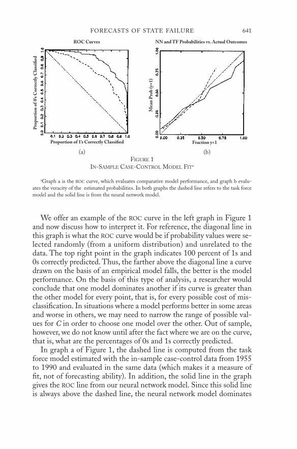
We offer an example of the ROC curve in the left graph in Figure 1and now discuss how to interpret it. For reference, the diagonal line inthis graph is what the ROC curve would be if probability values were se-lected randomly (from a uniform distribution) and unrelated to thedata. The top right point in the graph indicates 100 percent of 1s and0s correctly predicted. Thus, the farther above the diagonal line a curvedrawn on the basis of an empirical model falls, the better is the modelperformance. On the basis of this type of analysis, a researcher wouldconclude that one model dominates another if its curve is greater thanthe other model for every point, that is, for every possible cost of mis-classification. In situations where a model performs better in some areasand worse in others, we may need to narrow the range of possible val-ues for C in order to choose one model over the other. Out of sample,however, we do not know until after the fact where we are on the curve,that is, what are the percentages of 0s and 1s correctly predicted.

In graph a of Figure 1, the dashed line is computed from the taskforce model estimated with the in-sample case-control data from 1955to 1990 and evaluated in the same data (which makes it a measure offit, not of forecasting ability). In addition, the solid line in the graphgives the ROC line from our neural network model. Since this solid lineis always above the dashed line, the neural network model dominates


FIGURE 1IN-SAMPLE CASE-CONTROL MODEL FITa

aGraph a is the ROC curve, which evaluates comparative model performance, and graph b evalu-ates the veracity of the estimated probabilities. In both graphs the dashed line refers to the task forcemodel and the solid line is from the neural network model.

Proportion of 1’s Correctly Classified

(a)

Pro

port

ion

of0’

s Cor

rect

ly C

lass

ified

ROC Curves NN and TF Probabilities vs. Actual Outcomes

Mea

n P

rob

(y=1

)Fraction y=1

(b)

v53.i4.623.king 9/27/01 5:25 PM Page 641

the task force model, no matter what normative decision one mightmake about the costs of misclassification, C. Of course, since this graphis both fit and evaluated in the same data, it indicates that the neuralnetwork model fits the data better, not that it necessarily forecastsbetter.

Before moving to an evaluation of out-of-sample performance, wealso offer a test of the veracity of the estimated probabilities. A proba-bility that is accurate gives the fraction of times a state with the givencharacteristics will actually fail. To evaluate these probabilities, we sort estimated probabilities into bins of 0.1 width: [0,0.1),[0.1,0.2),…,[0.9,1]. For observations falling in each bin, we computethe mean predicted probability from the model (which will often besomewhere near the midpoint of each interval), as well as the observedfraction of 1s. If model probabilities are accurate, these two quantitiesshould be close: for example, if the probability of failure is forecast tobe 0.2 for a group of states, then about 20 percent of these states shouldactually fail. We then compare the two in graph b in Figure 1 to checkthe fit of the model in the training set (and below to evaluate the fore-casts in the test set). In this figure both models are fairly close to the45-degree line, indicating fairly accurate in-sample probabilities. Thegraph reveals the neural network model to have more informative prob-abilities (higher values), although these appear to be slightly underesti-mated (perhaps suggesting that the neural network priors should beadjusted to allow somewhat less smoothness, although we do not followup on this minor point).

We now consider the more important out-of-sample performance ofboth models. Figure 2 gives analogous graphs, estimated from the1955–90 data and evaluated in the 1991–98 data. When we refer to the“task force” model in these graphs, we make the case-control correc-tions described in Section III (otherwise, the probabilities in graph bwould be far worse).

As can be clearly seen, in the ROC graph a, the (solid) line for theneural network model is always above the (dashed) line representingtask force model. Thus, for every value of C, the neural network modelhas a higher percentage of 1s correctly predicted and a higher percent-age of 0s correctly predicted out of sample. Whatever one’s normativepreferences, therefore, the neural network model is superior to the(prior-corrected) task force model.

Graph b in Figure 2 indicates that the neural network probabilitiesare both more accurate (closer to the 45-degree line) and more infor-mative than those for the task force model (because they extend farther

642 WORLD POLITICS

v53.i4.623.king 9/27/01 5:25 PM Page 642

up the diagonal). The task force figures here are prior corrected, whichis why they do not extend as high as in Figure 1 and why they are any-where near the 45-degree line. Unfortunately, even with the correction,they do fairly poorly and are not accurate. Indeed, even prior correctionis insufficient, since the out-of-sample ranking of states in the proba-bility of failure is not preserved in the task force model. The dashed linedoubling back on itself means that higher estimated task force proba-bilities actually correspond to lower actual rates of state failure. Thesolid line, representing our neural network analysis, is not perfect, but itindicates that our estimated probabilities are at least monotonically re-lated to actual instances of state failure and are usually fairly close to thediagonal equality line. Taken together with the ROC graph, the availableevidence indicates that our neural network committee model offersout-of-sample forecasts that are better than the (prior-corrected) pre-dictions of the State Failure Task Force.41


41 Each of the methodological improvements we made to the task force model improved results overthe same model without that feature, and all were necessary to generate a model that dominated the(prior-corrected) task force model for any value of C. Of course, prior correction alone was sufficient toimprove a great deal on the original task force analysis. A rough ranking from most to least importantin changing the results is prior correction, neural networks, committee methods, the additional covari-ates, and multiple imputation for missing data.

FIGURE 2OUT-OF-SAMPLE GLOBAL MODEL FORECASTa

aGraph a is the ROC curve, which evaluates comparative model performance, and graph b evaluatesthe veracity of the estimated probabilities. In both graphs the dashed line refers to the task force model(although we also prior corrected, as in Section III) and the solid line is from the neural network model.

ROC Curves

Pro

port

ion

of0’

s Cor

rect

ly C

lass

ified

Proportion of 1’s Correctly Classified Fraction y = 1

Mea

n P

rob

(y =

1)

(b)(a)

NN and TF Probabilities vs. Actual Outcomes

v53.i4.623.king 9/27/01 5:25 PM Page 643

ADDITIONAL TESTS TO ENSURE AGAINST OVERFITTING

We conducted several additional tests to verify our claims to have builta model that can forecast more accurately and to have picked up somepiece of the underlying structure. In addition, we make these testssomewhat more difficult by using various subsets of our case-controldata for our training sets and subsets of the global data for our test set.Taking all this into account, we can think of no political science mod-eling exercise that has applied more stringent tests, whether for thepurpose of forecasting or for estimating causal effects.42

For our first test, we divided the country-years randomly betweentest and training sets and examined the ROC and probability graphs, asin Figures 1 and 2. In all cases, aside from what would be expected dueto random error, our neural network committee approach dominatedthe (prior-corrected) task force model. We also computed the marginaleffect graphs we report in Section VI and found that the causal struc-ture uncovered stays quite stable across the different random subsets.

We also use what we call the Stanford Test (so named because sev-eral Stanford faculty and fellows suggested it at a talk we gave there ona related subject), which combines a simple version of cross-validationwith out-of-sample verification. First, all countries are randomly di-vided into two groups, which we label A and B. The training and testsets are defined by dividing the sample chronologically at 1990, as be-fore. Then country group A in the training set is used to forecast coun-try group B in the test set. Similarly, country group B in the trainingset is used to forecast country group A in the test set. Hence, the fore-cast is both out of sample (to a future time) and out of space (to differ-ent countries). This is one of the hardest (reasonable) tests that can beconstructed to ascertain whether a statistical model has uncovered astable, causal structure and has not overfit the idiosyncrasies in the datathat do not persist. Although difficult, the Stanford Test is reasonableto apply to any analysis aimed at uncovering lawlike causal statementsor making genuine policy-relevant forecasts. (Although we do not pur-sue the possibility beyond the use of the test here, the procedure couldbe profitably generalized to all possible subsets A and B and formalizedto yield sampling probabilities.)

In the present case our test was made more difficult by the fact thatthere are only twenty-seven events in our test set after 1990 and thusonly about half that in country groups A and B. But even with the sam-

644 WORLD POLITICS

42 We summarize the results of these tests here, rather than presenting detailed accompanying fig-ures, since this would involve including numerous figures for each one presented in this paper.

v53.i4.623.king 9/27/01 5:25 PM Page 644

pling error induced by using only half the data at a time, the forecastingperformance, as judged by the ROC and probability graphs, and thecausal structure, as judged by our marginal effect plots, were all quiteconsistent with one another. In virtually all cases our neural networkcommittee approach dominated the (prior-corrected) task force model.

We also examined whether the substantive variables we measured,along with the estimated functional form, were sufficient to pick up theinformation represented in the country labels. That is, in almost anycountry-level analysis, a set of regional dummy variables will correlatehighly with the outcome variable. The key is determining whether one’ssubstantive variables pick up that variation, making the ad hoc idiosyn-crasies of including dummy variables unnecessary. In our case we com-pared the ROC curve for our model with one where we also added a setof regional dummy variables. Predictably, the model fit the in-sample(training set) much better. However, the key is that the out-of-sampleforecasts to our test set were considerably worse. This indicates that, in-deed, we were able to “get rid of proper nouns”:43 the dummy variablesare unnecessary and so our substantive variables apparently do not ex-clude any important structural components that correlate with thecountry names.

We also tried several measures of economic growth, because the lit-erature at least since Huntington44 has suggested that growth mightlead to state failure by empowering middle classes in authoritarianregimes. Unfortunately, we were unable to find evidence in support ofthis hypothesis or evidence that growth in any way adds forecastingpower to our models. We also tried adding the number of years sincethe last state failure, to model time-series dependence in the data,45 butwe found no evidence to support this variable either, although some ofthis effect might be represented in existing variables. In addition, wetried a time trend, but like the regional dummies it helped fit the in-sample data better but forecast considerably worse. We also examinedmany other individual variables from the task force data set, but findingno evidence that they could help in forecasting or would alter our sub-stantive conclusions, we excluded all of them.


43 Adam Przeworski and Henry Teune, The Logic of Comparative Social Inquiry (Malabar, Fla.:Krieger, 1982).

44 Samuel P. Huntington, Political Order in Changing Societies (New Haven: Yale University Press,1968).

45 Nathaniel Beck, Jonathan Katz, and Richard Tucker, “Taking Time Seriously: Time-Series-Cross-Section Analysis with a Binary Dependent Variable,” American Journal of Political Science 42(October 1998).

v53.i4.623.king 9/27/01 5:25 PM Page 645

The results of these successful validations from test sets defined onthe basis of time, random assignment, the Stanford Test, the regionaldummies, and other substantive variables cause us to be more confidentabout our ability to forecast and to believe we have found somethingapproximating causal structure. We could still be wrong, and past per-formance is no guarantee of future success; but it seems hard to arguethat these tests would not increase the chances that our model wouldhold for new data not yet collected. We think that future research bythe task force and others in this and related fields would benefit fromapplying these procedures.

V. SAMPLE FORECASTS

Studying individual forecast probabilities of state failure must be donecarefully, following the ideas about decision theory presented in SectionIV. A key issue is that a probability that may seem high from one per-spective could easily be considered low from another.

Our individual country-level forecasts easily distinguish countriesthat obviously do not have much risk of failure from those with somerisk, something that previous literature has not accomplished. For ex-ample, the published task force numbers—the only figures that havebeen used by policymakers—include a forecast that France would failin 1960 with an incredibly high 0.29 probability. In contrast, our modelforecasts a probability of state failure in France of nearly 0 for almostall years. More difficult is distinguishing among the countries withsome risk of failure. For example, with information available in 1964,our model gave a 0.35 probability of Uganda failing in 1966 (which isvery high for the probability of failure occurring in just one year).Uganda failed that year. By contrast, our model gave a forecast proba-bility of Kenya failing in that year of less than a third of the probabilityfor Uganda (Kenya did not fail).

Of course, these examples are anecdotes culled from the thousandsof predictions that come from our model and that cannot be fully pre-sented in this short article. Instead, we now summarize the numbers bygiving, in Table 4, our best and worst forecasts for all post-1990 coun-tries, based on the data from the case-control subset of countries up to1990. (Thus, our methods could be used to compute much better two-year-ahead forecasts than these by using all the information available;the 1998 forecasts, for example, are based on estimates from more thaneight years earlier.) For example, the ten country-years in the top leftsection of the table are those with the highest forecast probabilities of

646 WORLD POLITICS

v53.i4.623.king 9/27/01 5:25 PM Page 646

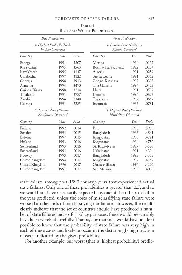
state failure among post-1990 country-years that experienced actualstate failures. Only one of these probabilities is greater than 0.5, and sowe would not have necessarily expected any one of the others to fail inthe year predicted, unless the costs of misclassifying state failure wereworse than the costs of misclassifying nonfailure. However, the resultsclearly indicate that the set of countries should have produced a num-ber of state failures and so, for policy purposes, these would presumablyhave been watched carefully. That is, our methods would have made itpossible to know that the probability of state failure was very high ineach of these cases and likely to occur in the disturbingly high fractionof cases indicated by the given probability.

For another example, our worst (that is, highest probability) predic-


TABLE 4BEST AND WORST PREDICTIONS

Best Predictions Worst Predictions

1. Highest Prob (Failure), 1. Lowest Prob (Failure),Failure Observed Failure Observed

Country Year Prob. Country Year Prob.

Senegal 1991 .5307 Mexico 1994 .0137Kyrgyzstan 1995 .4563 Bosnia-Herzegovina 1992 .0174Kazakhstan 1995 .4147 Algeria 1991 .0259Cambodia 1997 .4122 Sierra Leone 1991 .0312Georgia 1998 .3913 Congo-Kinshasa 1992 .0333Armenia 1994 .3470 The Gambia 1994 .0405Guinea-Bissau 1998 .3214 Haiti 1991 .0592Thailand 1991 .2787 Lesotho 1994 .0627Zambia 1996 .2348 Tajikistan 1992 .0667Georgia 1991 .2285 Indonesia 1997 .0781

2. Lowest Prob (Failure), 2. Highest Prob (Failure),Nonfailure Observed Nonfailure Observed

Country Year Prob. Country Year Prob.

Finland 1992 .0014 Peru 1998 .5955Sweden 1994 .0015 Bangladesh 1996 .4841Estonia 1997 .0015 Kyrgyzstan 1993 .4781Finland 1993 .0016 Kyrgyzstan 1994 .4752Switzerland 1993 .0016 St. Kitts-Nevis 1997 .4570Switzerland 1994 .0016 Uzbekistan 1991 .4394Norway 1993 .0017 Bangladesh 1995 .4355United Kingdom 1994 .0017 Kyrgyzstan 1997 .4187United Kingdom 1996 .0017 Guinea-Bissau 1996 .4110United Kingdom 1991 .0017 San Marino 1998 .4006

v53.i4.623.king 9/27/01 5:25 PM Page 647

tions among states that did not fail post-1990 are given in the bottomright of Table 4. If policy analysts had used our methods, they wouldhave expected to see some state failures among this group. Of course,the high probabilities without observed failures do not necessarily in-dicate a problem with our model, since the probabilities overall are ac-curate (that is, 30 percent of states with 0.3 probabilities really do fail30 percent of the time). If they were accurate for these countries, non-failure would be perfectly consistent with the model’s predictions forany one country at any one time, although for sets of countries theprobabilities ought to be realized in actual failures as predicted.

VI. EXPLORING EMPIRICAL REGULARITIES

In this section we discuss a variety of empirical regularities about statefailure uncovered by our analyses. These regularities are descriptive fea-tures of the underlying causal structure. The tests given in Section IVindicate that these empirical regularities are stable and predictable fea-tures of the world and account for some of our success at forecasting.They are not necessarily equivalent to causal effects, which require ad-ditional assumptions about counterfactuals, the validity of which nei-ther we nor the task force explores in any detail. For example, thatpeople with more education make more money is an empirical regular-ity. The claim that any one person, or people on average, would havemade more money if, ceteris paribus, they had received more educationis a causal claim. Causal claims are more difficult to substantiate be-cause they involve counterfactuals for which no direct evidence exists.46

Although different from causal effects, empirical regularities are stillvery valuable components of knowledge, since any theories of state fail-ure would need to be consistent with them. Similarly, any causal storywould need to account for these verified facts about the world.

Our procedure for summarizing the empirical regularities involvesusing marginal effect graphs—plots of the probability of state failure byone explanatory variable (at a time), while holding constant the set ofcontrol variables at different values to see how the relationships change.In addition, each marginal effect graph itself portrays an interaction be-tween democracy and another variable.

Figure 3 presents some of these marginal effect graphs. In eachgraph the predicted probability of state failure, computed from ourneural network committee model, is plotted vertically. One of the ex-planatory variables is plotted horizontally in each graph, with three

648 WORLD POLITICS

46 See King, Keohane, and Verba (fn. 11).

v53.i4.623.king 9/27/01 5:25 PM Page 648

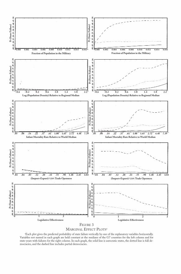
FIGURE 3MARGINAL EFFECT PLOTSa

aEach plot gives the predicted probability of state failure vertically by one of the explanatory variables horizontally.Variables not named in each graph are held constant at the medians of the G7 countries for the left column and forstate-years with failures for the right column. In each graph, the solid line is autocratic states, the dotted line is full de-mocracies, and the dashed line includes partial democracies.

0.000 0.002 0.004 0.006 0.008 0.010 0.012 0.014 0.016

Legislative Effectiveness Legislative Effectiveness

Pr (

Stat

e Fa

ilure

)

Pr (

Stat

e Fa

ilure

)P

r (St

ate

Failu

re)

(Import+Export)⁄GDP: Trade Openness (Import+Export)⁄GDP: Trade Openness

Pr (

Stat

e Fa

ilure

)

Infant Mortality Rate Relative to World Median

Pr (

Stat

e Fa

ilure

)

Pr (

Stat

e Fa

ilure

)

Infant Mortality Rate Relative to World Median

Fraction of Population in the Military Fraction of Population in the Military

Pr (

Stat

e Fa

ilure

)

Pr (

Stat

e Fa

ilure

)P

r (St

ate

Failu

re)

Pr (

Stat

e Fa

ilure

)

Log (Population Density) Relative to Regional MedianLog (Population Density) Relative to Regional Median–0.6 –0.2 0.2 0.6 1.0 1.4 1.8 2.2

.05 .08 .14 .22 .37 .61 1.00 1.65 2.72 4.48 7.39

.03 .04 .07 .12 .20 .33 .55 .90 1.48 2.45 4.03

0 1 2 3 0 1 2 3

.03 .04 .07 .12 .20 .33 .55 .90 1.48 2.45 4.03

–0.6 –0.2 0.2 0.6 1.0 1.4 1.8 2.2

.05 .08 .14 .22 .37 .61 1.00 1.65 2.72 4.48 7.39

0.000 0.002 0.004 0.006 0.008 0.010 0.012 0.014 0.016.00

.05

.10

.15

.20

.25

.30

.35

.40

.45

.50

.00

.05

.10

.15

.20

.25

.30

.35

.40

.45

.50

.00

.05

.10

.15

.20

.25

.30

.35

.40

.45

.50

.00

.05

.10

.15

.20

.25

.30

.35

.40

.45

.50

.00

.05

.10

.15

.20

.25

.30

.35

.40

.45

.50

.00

.05

.10

.15

.20

.25

.30

.35

.40

.45

.50

.00

.05

.10

.15

.20

.25

.30

.35

.40

.45

.50

.00

.05

.10

.15

.20

.25

.30

.35

.40

.45

.50

.00

.05

.10

.15

.20

.25

.30

.35

.40

.45

.50

.00

.05

.10

.15

.20

.25

.30

.35

.40

.45

.50

v53.i4.623.king 9/27/01 5:25 PM Page 649

lines drawn corresponding to full democracies (dotted), partial democ-racies (dashed), and autocracies (solid). The first column holds controlvariables (those not named on each graph) constant at the median valueof the G7 countries (except for the U.S., which is not included in thetask force data). The second column holds constant control variables atthe median for all countries with state failures. The graphs with con-trols held constant at the global median are similar to those in the sec-ond column, and so we do not present these. In addition, although ingeneral with flexible models like neural networks holding constant, thecontrol values at even slightly different values can result in very differ-ent looking marginal effect plots, such is less likely to be the case withour models since our priors impose smoothness on the functional form.(We exclude confidence intervals from these graphs for visual clarity,but all are sufficiently narrow to make the general interpretations fromthese lines reliable.)

The striking difference between the first and second columns of thisgraph shows that our model picks up the obvious differences betweenmajor industrial democracies and other countries as interactions amongsubstantive variables, rather than as indicator variables with country la-bels. Of all the variables examined in the first column, only very highlevels of infant mortality and, to some degree, very low levels of tradeopenness and ineffective legislatures increase the probability of statefailure to any significant level. The infant mortality result especially isfairly striking: only states with governments that are sufficiently com-petent to keep infant mortality below the global median have compar-atively low probabilities of state failure; other countries, even when theyare alike in all other measured respects to the G7, have substantialprobabilities of failure (as high as 0.25).

The second column represents time effects for countries that havevalues of their control variables like the median of those with state fail-ures. The fact that these graphs are so similar to ones drawn on thebasis of the global medians (not shown) indicates the stability and gen-eral applicability of the large effects witnessed there. Apparently, themain differences in the size and nature of the effects across the sampleof countries is between the G7 and everywhere else. An obvious effectoutside the G7 is the similar effect of democracy: for most of the rangesof all of the variables, partial democracies have a higher risk of failurethan either full democracies or autocracies. Most often, autocracieshave even lower risks than full democracies, although the differenceshere are mostly very small. We now interpret this effect along with thatfor legislative effectiveness in the bottom right corner of the figure. The

650 WORLD POLITICS

v53.i4.623.king 9/27/01 5:25 PM Page 650

story is similar to accounts such as Hibbs, Gurr, and Muller andWeede;47 what our data add to these is the qualification that it does notapply to countries when holding constant other variables at the level ofthe G7. That is, it is not only that the G7 countries are different or thatthey have some unmeasured characteristics that account for this differ-ence; it is instead that when the control variables take on values similarto those in the G7, even for non-G7 countries, this usual story aboutdemocracy is greatly reduced.

One version of this story is as follows.48 Autocracies are countriesthat have repressive central governments. Since dissent is nearly impos-sible, little conflict of any kind, much less state failure, is observed. Suchdifferences between the government and the people as may exist are notexpressed. In contrast, in partial democracies differences between thepeople and the government are publicly revealed to some degree. How-ever, because the institutions of democracy in partial democracies arenot capable of adjusting government policy quickly enough, public at-titudes can move far from the position of the government and staythere for a sustained period of time. In some cases, when the govern-ment cannot control this public conflict, the risk of state failure in-creases. We measure finer gradations of degrees of democracy in thepresent framework with the legislature effectiveness measure, which in-dicates the degree to which the legislature is channeling politicaldissent through electoral politics. The more this process is institution-alized, the lower the risks of state failure. Countries that are classified asfull democracies typically have high legislative effectiveness as well asmany of the other related attributes. Since public attitudes and govern-ment policy in these countries cannot stray far from one another forlong, the risks of state failure drop to low levels, even though there areexceptions. (Clearly this is a very different story from that told by theresults and arguments of the democratic peace literature, where themore democracy the better the chances of reducing conflict betweennations.)49


47 Douglas A. Hibbs Jr., Mass Political Violence: A Cross-National Causal Analysis (New York: Wiley,1973); Ted Robert Gurr, “Persistence and Change in Political Systems, 1800–1971,” American Politi-cal Science Review 68 (December 1974); Edward N. Muller and Erich Weede, “Cross-National Varia-tion in Political Violence: A Rational Action Approach,” Journal of Conflict Resolution 34 (December1990).

48 See, for example, Huntington (fn. 44); Ted Robert Gurr, “Why Minorities Rebel: A GlobalAnalysis of Communal Mobilization and Conflict since 1945,” International Political Science Review14, no. 2 (1993); R. J. Rummell, “Democracy, Power, Genocide, and Mass Murder,” Journal of ConflictResolution 39 (March 1995).

49 See also Edward Mansfield and Jack Snyder, “Democratization and War,” Foreign Affairs 74(1995).

v53.i4.623.king 9/27/01 5:25 PM Page 651

Just as having a gun in a household is a risk factor for murder andsuicide, the first graph in the second column of Figure 3 indicates thatlarger military populations are a risk factor for state failure. It is notclear whether this is because governments that fear failure increase thesize of their military in anticipation or whether larger fractions of thepopulation belonging to the military means that there are more poten-tial dissenters with access to weapons. Either way (and in all likelihood,both factors are operating), this result may provide additional motiva-tion for the ongoing movement of the international community towardconcepts of “human security.”50 Note also that most of the conditionaleffect of this variable occurs when the military fraction of the popula-tion is relatively small, with the effect still increasing but at a muchslower rate thereafter. Although this may suggest strategies for design-ing aid efforts that can achieve the largest effect for each dollar spent,further research would be required first.

The second row of the second column of Figure 3 shows that therisk of failure increases gradually with population density. This is afairly conventional result: people need to interact before they startfighting, but it could of course be some other characteristic of denselypopulated nations that is operating.

The third row illustrates the effects of infant mortality in partial de-mocracies sharply increasing the risks of state failure and then levelingoff. Infant mortality is a often a good proxy for the competence of thestate and it clearly picks this up here. When the infant mortality rate isequal to the world median or worse (a value of 1 or greater on the hor-izontal axis), the marginal probability of state failure is approximatelyconstant. However, in those countries where infant mortality is lower(to the left of 1)—and this is often a direct result of governmental in-tervention—the probability of state failure drops precipitously. Infantmortality is lower in most Western democracies, but there are numer-ous exceptions, most of which support the role of this variable as ameasure of state competence.51

652 WORLD POLITICS

50 For example, Lincoln C. Chen, “Human Security: Concepts and Approaches,” in T. Matsumaeand Lincoln C. Chen, eds., Common Security in Asia: New Concepts of Human Security (Tokyo: TokyoUniversity Press, 1995); Gary King and Christopher Murray, “Rethinking Human Security,” PoliticalScience Quarterly (forthcoming), preprint available at http://gking.harvard.edu.

51 For example, infant mortality in Cuba, where the government is so involved that the minister ofhealth chairs a separate meeting to investigate the case of each infant who dies in the country, is lowereven than the U.S. Some exceptions would include cases where natural disasters overwhelm the re-sources of even the most conscientious governments. Other exceptions include states where targetedinterventions, such as by the World Health Organization, reduce infant mortality without as muchhelp from the government involved (Ghana may be an example of this).

v53.i4.623.king 9/27/01 5:25 PM Page 652

The task force’s choice of a trade openness variable reflects the opti-mistic hypothesis that foreign policies designed to open markets mightalso reduce the incidence of state failure. We have found little directsupport for this idea in the literature, but a number of related variablesare relevant. For example, O’Kane52 uses export specialization (the per-centage of total export revenue derived from the largest single source ina country) to predict the probability of a coup. Her theory is that over-specialization leads to income instability, which in turn causes frustra-tion, low levels of development, and reduced governmental legitimacy.53

Export specialization is correlated with trade openness since countriesthat derive most of their GDP from a single export also receive most oftheir consumer goods and a lot of their food from abroad and so havehigh scores on the trade openness variable. This is consistent with ourresults, to which we now turn.

We find that high levels of trade openness are associated with theprobability of state failure, but with virtually all of the effect occurringin nations already having extremely high degrees of openness. Thisnonlinear trade openness result reveals significant biases in the taskforce’s logit results in Table 1: over most of the range there is no rela-tionship between trade openness and state failure. What the logitmodel is picking up (and incorrectly attributing to the entire range) isthe effect of outlier countries, the lower probability of state failure incountries with larger trading businesses than local economies (that is,when the horizontal axis is to the right of 1). These otherwise unex-pectedly wealthy countries include the oil-exporting states and stateslike Singapore that occupy the “middleman” trading positions.54

We reemphasize that these empirical regularities are marginal effectplots; they are obviously not the results of randomized experiments orof an observational study where we know the explanatory variables areexogenous. They are “partial” (or “direct”) causal effects that control forsome of the consequences of the causal variables being studied. Ourtests indicate that stable structures underlie these data, no matter howwe look at them, but whether these should be relied on to draw causalinferences or change foreign aid policy must be the subject of additionalstudy. Since foreign aid decisions are easier to identify and their moti-


52 Rosemary O’Kane, The Likelihood of Coups (Averbury: Aldershot, 1987).53 For a contrary view, see Collier (fn. 32).54 It is also worth noting that this result unfortunately blurs the distinction between variable-based

explanations, which we prefer, and country-based “proper noun” stories. More generally, this result alsosuggests, as is the case, that logistic regression results are more sensitive to outliers than are neural net-works. Whereas an outlier can throw off the entire logistic curve, neural networks, by contrast, willusually map outliers separately and localize their effects to small pieces of the functional form.

v53.i4.623.king 9/27/01 5:25 PM Page 653

vations could be (and have been) the subject of much analysis, we havea chance of ascertaining where foreign aid dollars would have theirlargest effects.

VII. CONCLUDING REMARKS

Although we find problems in the work of the State Failure Task Forcethat lead to overly large forecasts, exaggerated assessments of forecast-ing performance, and biased causal inferences, we wish to emphasizethat it has nonetheless accomplished a great deal. The members havemerged their deep knowledge of state failure to create a remarkable,carefully documented data set. The many millions of dollars invested increating these data far exceed the resources spent on any other data seton state failure, indeed, on almost all other data sets in the discipline.The data set codifies numerous qualitative insights and knowledgefrom a diverse variety of area studies and other experts brought in toadd their expertise to individual variables. The result is that it is nowpossible to test numerous theories systematically, many for the firsttime. Even their favored model, when appropriately corrected, per-forms quite well. We were able to outperform even corrected versionsof their forecasting model, but only by introducing new methods tobuild on what the task force had already produced.

We have no doubt that further work in data, methodological inno-vation, theory, or area studies would produce better forecasts than eventhose offered here. We hope this line of research also helps the aca-demic community and policymakers to understand, forecast, and ad-dress the critical problem of state failure.

As discussed in the introduction, the task force’s definition of statefailure is highly heterogeneous, and so progress would likely be madeby breaking down this variable into its component parts. We concludehere with a related issue and suggestion for further research. Althoughall forecasts reported here are “real” in the sense of being tested out ofsample, with data only available at least two years prior to the potentialevent, the logical status of each of the variables in the task force defini-tions is not entirely what was intended. In some sense, the explanatoryvariables (infant mortality, partial democracy, legislative [in]effective-ness, and so on) are really indirect indicators that the state has alreadyfailed, whereas their heterogeneous dependent variables (genocide, dis-ruptive regime transitions, and revolutionary wars aimed at displacingthe regime) are not really measures of state failure but instead are indi-cators of some of the disastrous consequences of state failure. Studies in-

654 WORLD POLITICS

v53.i4.623.king 9/27/01 5:25 PM Page 654

tending to forecast and explain the consequences of state failure are ob-viously important,55 but so would be a study that tried to predict andexplain the onset of state failure—the collapse of the central authoritystructures of the state. To do this would require a different strategy fordata collection than that pursued by the task force and a more tailored,operational definition of state failure and the institutionalization, legit-imacy, and authority of the state.

APPENDIX 1: STATE FAILURE DATA

The task force data set we received includes 1,231 variables for 195 dis-tinct countries between 1955 and 1998. Compiled from many sources,the data set provides information on political, sociological, economic,cultural, religious, educational, demographic, environmental, and publichealth characteristics of each country with a population greater than halfa million. The data set contains information from commercial sourcesand from sources in the public domain, and some of the data were cre-ated or corrected by the task force; none of the data were classified.

While the task force has made older versions of its dependent vari-able available on the web, it has until now prevented others from ac-cessing the rest of its extensive data collection and (for parts) has notindicated from which commercial source it can be purchased and pre-cisely how to merge the different sources to re-create their data set.Upon publication of this article, the full task force data set to which wehad access will be available at http://gking.harvard.edu. The task forcecontinues to update and improve its data, and we encourage it to releasesubsequent versions so that the scholarly community may continue tobenefit from its efforts and further improve forecasts of state failure.

This appendix lists some of the representative variables for interestedreaders. Due to space limitations, it is impossible to give detailed infor-mation on the variables (for example, measurement) here, and theoriginal data set should be consulted for that purpose. A complete listof data sources appears in the task force report.56

The data set includes such variables as country code/name, year, geo-graphic region, case-control indicators; information on leaders (name,education level/discipline, etc.); characteristics of the ruling elite; ethnic/


55 See Robert Melson, Revolution and Genocide: The Origins of the Armenian Genocide and the Holo-caust (Chicago: University of Chicago Press, 1992); Matt Krain, “State Sponsored Mass Murder: TheOnset and Severity of Genocides and Politicides,” Journal of Conflict Resolution 41 ( June 1997); Ben-jamin Valentino, “Final Solutions: The Causes of Genocide and Mass Killing,” Security Studies 9(Spring 2000).

56 Esty et al. (fn. 1, 1998).

v53.i4.623.king 9/27/01 5:25 PM Page 655

linguistic/religious groups; population (sizes, composition, density); in-come, GDP/GNP (various measures), consumption, government expen-ditures, money supply, price indexes, foreign investment, imports/exports, foreign aid, exchange rates, interest rates; labor force (sizes,composition, occupational distribution); democracy measures, defenseexpenditures, military expenditures, assassinations, coups, generalstrikes, guerrilla warfare, government crises, purges, riots, revolutions,antigovernment demonstrations, seats in the legislature, legislature size,legislative effectiveness, competitiveness of nominating process, partycoalitions, party legitimacy, type of regime, major constitutionalchanges, cabinet size, Freedom House political rights index, FreedomHouse civil liberties index, historical conflict information, regime dura-bility; school enrollment, illiteracy rate, pupil-teacher ratios, public ed-ucation expenditures; safe water access, natural disasters, cropland area,crop yield, fertilizer consumption, rail mileage, forest and woodland in-formation; physicians per capita, mortality rate, life expectancy, fertilityrate, information on AIDS, standard of living index, birthrate, deathrate; crime statistics; newspaper circulation; modernization and post-modernization indexes, cultural zone, and a subjective well-being score.

APPENDIX 2: A BRIEF INTRODUCTION TO

NEURAL NETWORK MODELS

Binary outcome variables are modeled with a Bernoulli probability dis-tribution, which means simply that the outcome variable Y takes on thevalue Y = 1 (for state failure) with probability π and Y = 0 (no failure)with probability 1– π. The only assumptions so far are that the defini-tion of the two categories are mutually exclusive and exhaustive, bothof which hold automatically because of the definition of state failure.

The question to be answered by statistical analysis is what the prob-ability of state failure (π) is for possible configurations of values of theexplanatory variables, x. In logistic regression, π is assumed to vary withx according to a logistic function, π = 1/(1 + e–α–xβ). That is, if we plot-ted x horizontally and π vertically, the logistic function would look likean escalator with π approaching 0 at the bottom and 1 at the top. Thedirection (from top left to bottom right or top right to bottom left) andsteepness of the escalator-shaped curve are determined by the values ofthe parameters α and β.

Choosing a logistic regression model is precisely the choice of a spe-cific family of possible curves, specific members of which are determinedby the values of α and β. Logistic regression analysis then involves

656 WORLD POLITICS

v53.i4.623.king 9/27/01 5:25 PM Page 656

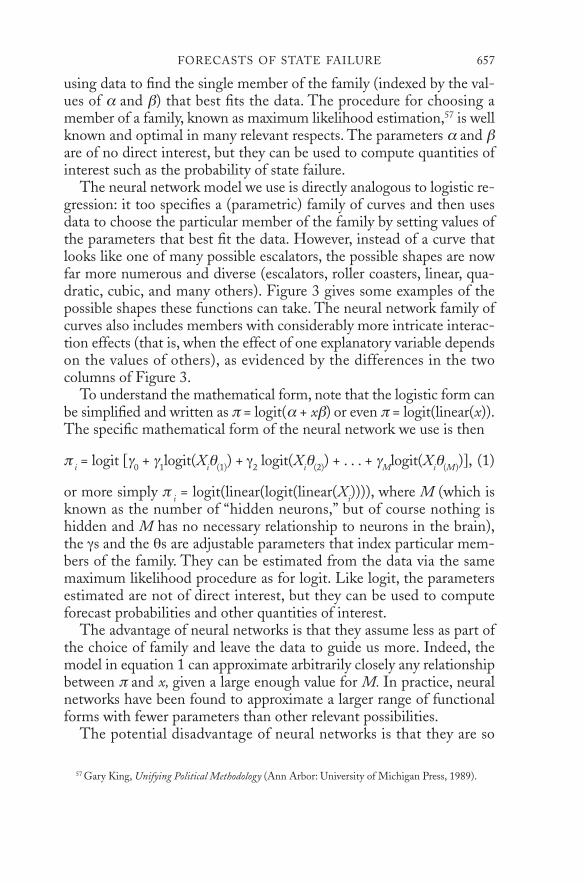
using data to find the single member of the family (indexed by the val-ues of α and β) that best fits the data. The procedure for choosing amember of a family, known as maximum likelihood estimation,57 is wellknown and optimal in many relevant respects. The parameters α and βare of no direct interest, but they can be used to compute quantities ofinterest such as the probability of state failure.

The neural network model we use is directly analogous to logistic re-gression: it too specifies a (parametric) family of curves and then usesdata to choose the particular member of the family by setting values ofthe parameters that best fit the data. However, instead of a curve thatlooks like one of many possible escalators, the possible shapes are nowfar more numerous and diverse (escalators, roller coasters, linear, qua-dratic, cubic, and many others). Figure 3 gives some examples of thepossible shapes these functions can take. The neural network family ofcurves also includes members with considerably more intricate interac-tion effects (that is, when the effect of one explanatory variable dependson the values of others), as evidenced by the differences in the twocolumns of Figure 3.

To understand the mathematical form, note that the logistic form canbe simplified and written as π = logit(α + xβ) or even π = logit(linear(x)).The specific mathematical form of the neural network we use is then

π i = logit [γ0 + γ1logit(Xiθ(1)) + γ2 logit(Xiθ(2)) + . . . + γMlogit(Xiθ(M))], (1)

or more simply π i = logit(linear(logit(linear(Xi)))), where M (which isknown as the number of “hidden neurons,” but of course nothing ishidden and M has no necessary relationship to neurons in the brain),the γs and the θs are adjustable parameters that index particular mem-bers of the family. They can be estimated from the data via the samemaximum likelihood procedure as for logit. Like logit, the parametersestimated are not of direct interest, but they can be used to computeforecast probabilities and other quantities of interest.

The advantage of neural networks is that they assume less as part ofthe choice of family and leave the data to guide us more. Indeed, themodel in equation 1 can approximate arbitrarily closely any relationshipbetween π and x, given a large enough value for M. In practice, neuralnetworks have been found to approximate a larger range of functionalforms with fewer parameters than other relevant possibilities.

The potential disadvantage of neural networks is that they are so


57 Gary King, Unifying Political Methodology (Ann Arbor: University of Michigan Press, 1989).

v53.i4.623.king 9/27/01 5:25 PM Page 657

flexible that they can fit idiosyncrasies in the data rather than structuralfeatures that persist, although we guard against this with the methodsoffered in Section IV. In only rare situations will a neural networkmodel be outperformed by a logistic model. Indeed, choosing a logisticmodel over a neural network model would be appropriate mainly ifthere existed strong substantive theory that ruled out all members ofthe neural network family of curves other than the logistic. In fact,however, we know of no such substantive theory of state failure thateven addresses these issues and so there exists little justification for logitover neural networks. See King, Beck, and Zeng58 for more detailsalong the same lines and Bishop59 for a complete presentation of neuralnetworks.

658 WORLD POLITICS

58 Beck, King, and Zeng (fn. 35).59 Bishop (fn. 38).

v53.i4.623.king 9/27/01 5:25 PM Page 658

Improving Forecasts of State Failure - Gary King - Harvard University

Documents

Transcript of Improving Forecasts of State Failure - Gary King - Harvard University