
Enhancing lives and improving drugs Update September 8, 2011.

Improving Efficiency and
Enhancing Utilizability of
Media-on-Demand Systems
Dem Fachbereich 03 — Mathematik/Informatik —
der Universität Bremen
zur Erlangung des akademischen Grades eines
Doktor-Ingenieurs (Dr.-Ing.)
eingereichte
Dissertation
von
Dipl.-Inf. Boris Nikolaus
aus
Berlin, Deutschland
Datum der Einreichung: 2008/07/01
Referent: Prof. Dr. Ute Bormann, Universität Bremen
Koreferent: Prof. Dr. Jörg Ott, Helsinki University of Technology
Tag der mündlichen Prüfung: 2008/09/05

Abstract
Nikolaus, Boris:
Improving Efficiency and Enhancing Utilizability of Media-on-Demand Systems
Media-on-demand is a method which extends traditional media transmissions by an important ser-
vice: While consumers depend on the schedule of broadcasting organizations in case of traditional
media transmissions like television or radio, they are granted the possibility to select a media
stream from the offer of the provider and request it at arbitrary time in case of media-on-demand.
Certainly, this surplus service creates additional requirements to the sender and receiver sys-
tems and to the network between these systems, especially when a large number of receiver
systems are simultaneously active. To keep these requirements low, many advanced media-on-
demand systems and transmission techniques have been proposed in recent years. Besides of
following different approaches, these systems differ by their goals and focus, their efficiency and
utilizability, and each of them brings its own advantages and drawbacks with it.
The aim of the present thesis is to improve the efficiency of media-on-demand transmissions
and to enhance the utilizability of media-on-demand systems. To achieve these goals, many media-
on-demand systems have been analyzed, and from the gained experience and knowledge, a new
and improved system has been developed. This new system distinguishes itself from existing
systems by incorporating nearly any of the advantages and extensions of the other systems while
operating at an efficiency near to the theoretical optimum and by providing a high flexibility and
robustness at the same time. To prove the practical benefit of the proposed system in real en-
vironments, an embedding into an existing real-time transport protocol has been proposed and a
comparison of the cost-effectiveness opposed to traditional media-on-demand systems has been
provided.
Media-on-Demand, Video-on-Demand, Interactive TV, Media Streaming


Zusammenfassung
Nikolaus, Boris:
Improving Efficiency and Enhancing Utilizability of Media-on-Demand Systems
Steigerung der Effizienz und Verbesserung der Einsetzbarkeit von Media-on-Demand-Systemen
Media-on-Demand ist ein Verfahren, das traditionelle Medienübertragungen um einen wichtigen
Dienst erweitert: Während bei traditionellen Medienübertragungen wie z. B. Fernsehen und Ra-
dio die Sendeanstalten das Programm festlegen, ist es dem Konsument bei Media-on-Demand
möglich, einen Medienstrom aus dem Angebot des Anbieters auszuwählen und zu beliebiger Zeit
anzufordern.
Dieser Mehrwert erzeugt natürlich zusätzliche Anforderungen an die Sende- und Empfangs-
systeme und an das Netzwerk zwischen diesen Systemen, insbesondere wenn eine große An-
zahl von Empfangssystemen zeitgleich aktiv sein kann. Um die Anforderungen möglichst gering
zu halten, wurden in den letzten Jahren viele hochentwickelte Media-on-Demand-Systeme und
-Übertragungstechniken vorgestellt. Neben der Verfolgung verschiedener Ansätze unterscheiden
sich diese Verfahren auch in ihren Zielsetzungen, Schwerpunkten, ihrer Effizienz sowie Einsetz-
barkeit und bringen unterschiedliche, systemimmanente Vor- und Nachteile mit sich.
Die vorliegende Arbeit hat die Zielsetzung, die Effizienz von Media-on-Demand-Übertragungen
zu steigern und die Einsetzbarkeit von Media-on-Demand-Systemen zu verbessern. Um diese Zie-
le zu erreichen, wurden eine große Anzahl bestehender Media-on-Demand-Verfahren analysiert
und mit den daraus gewonnenen Erfahrungen und Erkenntnissen ein neues, verbessertes System
entwickelt. Dieses neue System zeichnet sich dadurch aus, dass es nahezu alle Vorteile und Er-
weiterungen der bestehenden Verfahren in sich vereint, eine Effizienz nahe dem theoretischen
Optimum besitzt und zugleich äußerst flexibel und robust in seinem Einsatz ist. Um den prakti-
schen Nutzen des Systems in realen Einsatzgebieten zu belegen, wurde zusätzlich eine Einbettung
in ein existierendes Echtzeittransportprotokoll vorgestellt und in einem Kostenvergleich die wirt-
schaftliche Rentabilität der von traditionellen Media-on-Demand-Systemen gegenübergestellt.
Media-on-Demand, Video-on-Demand, interaktives Fernsehen, Medienstromübertragung


Acknowledgments
This thesis is the result of the research I carried out from 1998 to 2007 on the topic of media-on-
demand. Although I am the sole author of this thesis, many people have contributed to it, to my
education and to my live, and it is my greatest pleasure to take this opportunity to thank them.
First and foremost, I would like to express my greatest gratitude to Prof. Dr.-Ing. Jörg Ott. After
receiving much guidance from him when I wrote my diploma thesis at the Technische Universität
Berlin, I am very pleased that he decided to continue attending my academic career. Although liv-
ing about 300 km apart (and since 2005 even around 1100 km), he managed to meet me countless
times (while being always available by telephone) for our innumerable and fruitful discussions
which not only brought new ideas and approaches into view but also delighted and motivated me
much to continue my work on this long and sometimes stubborn path.
Furthermore, it gives me great pleasure to thank Prof. Dr.-Ing. Ute Bormann and Prof. Dr.-
Ing. Carsten Bormann for participating in many enlightening discussions and for their organiza-
tional and professional guidance to a successful thesis.
Additionally, I would like to thank Prof. Dr.-Ing. Ute Bormann for accepting supervision of
this thesis and Prof. Dr.-Ing. Jörg Ott for taking the role of the second thesis advisor.
There is one other friend I owe special thanks: During countless meetings, I got an invaluable
help from Dipl.-Inf. Frank Tscheuschner by proofreading my publications and parts of this thesis,
making critical remarks and useful suggestions and besides this for improving my English. I
also would like to offer my thanks to Dipl.-Ing. Stefan Schwabe, Dipl.-Ing. Martina Liggesmeier,
Dipl.-Ing. Tobias Poschwatta and Dipl.-Wirtschaftsinf. (FH) Christian Zanoth for proofreading
this thesis.
Finally, I would like to thank my parents and especially my wife for their patience, their encour-
agement and all the support they gave me to perform my researches and to successfully complete
this thesis.

Contents
1 Introduction 1
1.1 Media-on-Demand . . . . . . . . . . . . . . . . . . . . . . . . . . . . . . . . . 2
1.2 Motivation for Media-on-Demand . . . . . . . . . . . . . . . . . . . . . . . . . 4
1.3 Scope of this Thesis . . . . . . . . . . . . . . . . . . . . . . . . . . . . . . . . . 7
1.4 Structure of this Thesis . . . . . . . . . . . . . . . . . . . . . . . . . . . . . . . 9
2 Media-on-Demand Systems 11
2.1 Functioning and Capabilities of Media-on-Demand Systems . . . . . . . . . . . 12
2.2 Structure of Media-on-Demand Systems . . . . . . . . . . . . . . . . . . . . . . 13
2.2.1 Sender-Side Components of a Media-on-Demand System . . . . . . . . 15
2.2.2 Receiver-Side Components of a Media-on-Demand System . . . . . . . . 20
2.3 Topology of Media-on-Demand Systems . . . . . . . . . . . . . . . . . . . . . . 21
2.4 Classification of Media Transmission Systems . . . . . . . . . . . . . . . . . . . 25
2.4.1 Technical Classification of Media Transmission Systems . . . . . . . . . 26
2.4.2 Functional Classification for Media Transmission Systems . . . . . . . . 32
2.5 Media Content and Format . . . . . . . . . . . . . . . . . . . . . . . . . . . . . 37
2.5.1 Structure of Media Content . . . . . . . . . . . . . . . . . . . . . . . . . 38
2.5.2 Content of Media Streams . . . . . . . . . . . . . . . . . . . . . . . . . 39
2.5.3 Media Encodings . . . . . . . . . . . . . . . . . . . . . . . . . . . . . . 39
2.6 Summary . . . . . . . . . . . . . . . . . . . . . . . . . . . . . . . . . . . . . . 41
3 Media Transmission Schemes 43
3.1 Efficiency of Media Transmission Schemes . . . . . . . . . . . . . . . . . . . . 45
3.1.1 Request Pattern for Media-on-Demand Transmissions . . . . . . . . . . 46
3.1.2 Minimum Required Bandwidth for Reactive Transmission Schemes . . . 48
3.1.3 Minimum Required Bandwidth for Pro-Active Transmission Schemes . . 50
3.1.4 Efficiency Graphs . . . . . . . . . . . . . . . . . . . . . . . . . . . . . . 52
3.2 Traditional Media Transmission Schemes . . . . . . . . . . . . . . . . . . . . . 53

vi CONTENTS
3.2.1 Single Broadcast . . . . . . . . . . . . . . . . . . . . . . . . . . . . . . 53
3.2.2 Personal Tape Archive . . . . . . . . . . . . . . . . . . . . . . . . . . . 54
3.2.3 Video Rental Stores and Media Libraries . . . . . . . . . . . . . . . . . 55
3.2.4 Complete Preloading of Media Streams . . . . . . . . . . . . . . . . . . 55
3.2.5 Summary of Traditional Media Transmission Schemes . . . . . . . . . . 56
3.3 Reactive Media-on-Demand Transmission Schemes . . . . . . . . . . . . . . . . 57
3.3.1 Point-to-Point Transmissions . . . . . . . . . . . . . . . . . . . . . . . . 57
3.3.2 Batching . . . . . . . . . . . . . . . . . . . . . . . . . . . . . . . . . . 59
3.3.3 Adaptive Piggy-Backing . . . . . . . . . . . . . . . . . . . . . . . . . . 62
3.3.4 Patching . . . . . . . . . . . . . . . . . . . . . . . . . . . . . . . . . . . 63
3.3.5 Tapping . . . . . . . . . . . . . . . . . . . . . . . . . . . . . . . . . . . 66
3.3.6 Merging . . . . . . . . . . . . . . . . . . . . . . . . . . . . . . . . . . . 69
3.3.7 Virtual Batching . . . . . . . . . . . . . . . . . . . . . . . . . . . . . . 71
3.3.8 Peer-to-Peer Networks . . . . . . . . . . . . . . . . . . . . . . . . . . . 73
3.3.9 Comparison of Reactive Transmission Schemes . . . . . . . . . . . . . . 75
3.4 Non-Segmenting Pro-Active Transmission Schemes . . . . . . . . . . . . . . . . 78
3.4.1 Round-Robin Broadcasting . . . . . . . . . . . . . . . . . . . . . . . . . 79
3.4.2 Staggered Broadcasting . . . . . . . . . . . . . . . . . . . . . . . . . . 80
3.4.3 Comparison of Non-Segmenting Pro-Active Transmission Schemes . . . 81
3.5 Size-Based Segmenting Transmission Schemes . . . . . . . . . . . . . . . . . . 82
3.5.1 Pyramid Broadcasting . . . . . . . . . . . . . . . . . . . . . . . . . . . 84
3.5.2 Permutation-Based Pyramid Broadcasting . . . . . . . . . . . . . . . . . 85
3.5.3 Skyscraper Broadcasting . . . . . . . . . . . . . . . . . . . . . . . . . . 86
3.5.4 Mayan Temple Broadcasting . . . . . . . . . . . . . . . . . . . . . . . . 89
3.5.5 Client-Centric Approach . . . . . . . . . . . . . . . . . . . . . . . . . . 90
3.5.6 Greedy Disk-Conserving Broadcasting . . . . . . . . . . . . . . . . . . 91
3.5.7 Greedy Equal Bandwidth Broadcasting . . . . . . . . . . . . . . . . . . 93
3.5.8 Fibonacci Broadcasting . . . . . . . . . . . . . . . . . . . . . . . . . . . 95
3.5.9 Reliable Periodic Broadcasting/Generalized Fibonacci Broadcasting . . . 95
3.5.10 Comparison of Size-Based Segmenting Transmission Schemes . . . . . . 97
3.6 Bandwidth-Based Segmenting Transmission Schemes . . . . . . . . . . . . . . . 99
3.6.1 Harmonic Broadcasting . . . . . . . . . . . . . . . . . . . . . . . . . . 101
3.6.2 Cautious Harmonic Broadcasting . . . . . . . . . . . . . . . . . . . . . 102
3.6.3 Quasi-Harmonic Broadcasting . . . . . . . . . . . . . . . . . . . . . . . 104
3.6.4 Polyharmonic Broadcasting . . . . . . . . . . . . . . . . . . . . . . . . 104
3.6.5 Tailored Transmissions . . . . . . . . . . . . . . . . . . . . . . . . . . . 106

CONTENTS vii
3.6.6 Staircase Broadcasting . . . . . . . . . . . . . . . . . . . . . . . . . . . 108
3.6.7 Seamless Staircase Broadcasting . . . . . . . . . . . . . . . . . . . . . . 109
3.6.8 Comparison of Bandwidth-Based Segmenting Transmission Schemes . . 111
3.7 Frequency-Based Segmenting Transmission Schemes . . . . . . . . . . . . . . . 113
3.7.1 Harmonic Equal-Bandwidth Broadcasting . . . . . . . . . . . . . . . . . 114
3.7.2 Fast Broadcasting . . . . . . . . . . . . . . . . . . . . . . . . . . . . . . 114
3.7.3 Seamless Fast Broadcasting . . . . . . . . . . . . . . . . . . . . . . . . 117
3.7.4 Pagoda Broadcasting . . . . . . . . . . . . . . . . . . . . . . . . . . . . 118
3.7.5 New Pagoda Broadcasting . . . . . . . . . . . . . . . . . . . . . . . . . 119
3.7.6 Fixed Delay Pagoda Broadcasting . . . . . . . . . . . . . . . . . . . . . 121
3.7.7 Variable Bandwidth Broadcasting . . . . . . . . . . . . . . . . . . . . . 122
3.7.8 Greedy Broadcasting/Recursive Frequency Splitting . . . . . . . . . . . 124
3.7.9 Fuzzycast . . . . . . . . . . . . . . . . . . . . . . . . . . . . . . . . . . 125
3.7.10 Dual Broadcasting . . . . . . . . . . . . . . . . . . . . . . . . . . . . . 127
3.7.11 Comparison of Frequency-Based Segmenting Transmission Schemes . . 129
3.8 Reactive-Pro-Active-Hybrid Transmission Schemes . . . . . . . . . . . . . . . . 131
3.8.1 Unified Video-on-Demand Broadcasting . . . . . . . . . . . . . . . . . . 131
3.8.2 Batching Unified Video-on-Demand Broadcasting . . . . . . . . . . . . 131
3.8.3 Reactive Broadcasting . . . . . . . . . . . . . . . . . . . . . . . . . . . 132
3.8.4 Dynamic Skyscraper Broadcasting . . . . . . . . . . . . . . . . . . . . . 133
3.8.5 Partitioned Dynamic Skyscraper Broadcasting . . . . . . . . . . . . . . . 133
3.8.6 Universal Broadcasting . . . . . . . . . . . . . . . . . . . . . . . . . . . 135
3.8.7 Channel-Based Heuristic Distribution . . . . . . . . . . . . . . . . . . . 136
3.8.8 Comparison of Reactive-Pro-Active-Hybrid Transmission Schemes . . . 137
3.9 Summary . . . . . . . . . . . . . . . . . . . . . . . . . . . . . . . . . . . . . . 139
4 Generalized Greedy Broadcasting Scheme 143
4.1 Origin of Generalized Greedy Broadcasting . . . . . . . . . . . . . . . . . . . . 144
4.1.1 Requirements . . . . . . . . . . . . . . . . . . . . . . . . . . . . . . . . 144
4.1.2 Playback Function, Transmission Function and Cumulative Bandwidth
Function . . . . . . . . . . . . . . . . . . . . . . . . . . . . . . . . . . 145
4.1.3 Tree-Based Representation for Transmission Schemes . . . . . . . . . . 146
4.1.4 Greedy Broadcasting/Recursive Frequency Splitting Scheme . . . . . . . 149
4.2 Generalization of Greedy Broadcasting/Recursive Frequency Splitting . . . . . . 151
4.3 Efficiency Improvements . . . . . . . . . . . . . . . . . . . . . . . . . . . . . . 154
4.4 Increasing the Playback Delay . . . . . . . . . . . . . . . . . . . . . . . . . . . 157
4.4.1 Intention and Effects . . . . . . . . . . . . . . . . . . . . . . . . . . . . 158

viii CONTENTS
4.4.2 Transmission Function for Playback Delays . . . . . . . . . . . . . . . . 159
4.4.3 Application to the Generalized Greedy Broadcasting Scheme . . . . . . . 160
4.5 Reducing Segment Sizes . . . . . . . . . . . . . . . . . . . . . . . . . . . . . . 160
4.5.1 Intention and Effects . . . . . . . . . . . . . . . . . . . . . . . . . . . . 161
4.5.2 Transmission Function for Reduced Segment Sizes . . . . . . . . . . . . 163
4.5.3 Application to the Generalized Greedy Broadcasting Scheme . . . . . . . 163
4.6 Partial Preloading . . . . . . . . . . . . . . . . . . . . . . . . . . . . . . . . . . 164
4.6.1 Intention and Effects . . . . . . . . . . . . . . . . . . . . . . . . . . . . 164
4.6.2 Transmission Function for Partial Preloading . . . . . . . . . . . . . . . 167
4.6.3 Application to the Generalized Greedy Broadcasting Scheme . . . . . . . 167
4.7 Introducing Breaks into Transmissions . . . . . . . . . . . . . . . . . . . . . . . 168
4.7.1 Intention and Effects . . . . . . . . . . . . . . . . . . . . . . . . . . . . 168
4.7.2 Transmission Function for Insertion of Breaks . . . . . . . . . . . . . . . 168
4.7.3 Application to the Generalized Greedy Broadcasting Scheme . . . . . . . 170
4.8 Variable-Bit-Rate Media Transmissions . . . . . . . . . . . . . . . . . . . . . . 171
4.8.1 Smoothing Variable-Bit-Rate Media Streams . . . . . . . . . . . . . . . 171
4.8.2 Piecewise Smoothing of Variable-Bit-Rate Media Streams . . . . . . . . 172
4.8.3 Immediate Transmission of Variable-Bit-Rate Media Streams . . . . . . 173
4.8.4 Application to the Generalized Greedy Broadcasting Scheme . . . . . . . 173
4.9 Immediate Segment Reception . . . . . . . . . . . . . . . . . . . . . . . . . . . 175
4.9.1 Intention and Effects . . . . . . . . . . . . . . . . . . . . . . . . . . . . 175
4.9.2 Application to the Generalized Greedy Broadcasting Scheme . . . . . . . 176
4.10 Decoupled Channel-Bandwidth . . . . . . . . . . . . . . . . . . . . . . . . . . . 176
4.10.1 Intention and Effects . . . . . . . . . . . . . . . . . . . . . . . . . . . . 176
4.10.2 Application to the Generalized Greedy Broadcasting Scheme . . . . . . . 178
4.11 Channel Sharing . . . . . . . . . . . . . . . . . . . . . . . . . . . . . . . . . . . 178
4.11.1 Intention and Effects . . . . . . . . . . . . . . . . . . . . . . . . . . . . 178
4.11.2 Application to the Generalized Greedy Broadcasting Scheme . . . . . . . 179
4.12 Enhanced Startup . . . . . . . . . . . . . . . . . . . . . . . . . . . . . . . . . . 180
4.12.1 Intention and Effects . . . . . . . . . . . . . . . . . . . . . . . . . . . . 180
4.12.2 Modifying Transmission Schedules . . . . . . . . . . . . . . . . . . . . 181
4.12.3 Improved Startup Enhancement Algorithm . . . . . . . . . . . . . . . . 183
4.12.4 Lowering the Efficiency to Improve the Startup . . . . . . . . . . . . . . 187
4.13 Enhanced Termination . . . . . . . . . . . . . . . . . . . . . . . . . . . . . . . 188
4.13.1 Intention and Effects . . . . . . . . . . . . . . . . . . . . . . . . . . . . 189
4.13.2 Application to Generalized Greedy Broadcasting Scheme . . . . . . . . . 190

CONTENTS ix
4.14 Seamless Media Change . . . . . . . . . . . . . . . . . . . . . . . . . . . . . . 190
4.14.1 Intention and Effects . . . . . . . . . . . . . . . . . . . . . . . . . . . . 190
4.14.2 Application to Generalized Greedy Broadcasting Scheme . . . . . . . . . 191
4.15 Change of Media Bit Rate for Ongoing Transmissions . . . . . . . . . . . . . . . 193
4.15.1 Intention and Effects . . . . . . . . . . . . . . . . . . . . . . . . . . . . 193
4.15.2 Application to Generalized Greedy Broadcasting Scheme . . . . . . . . . 195
4.15.3 Alternative Solution: Layered Media Encodings . . . . . . . . . . . . . . 195
4.16 Change of Sender Bandwidth and Playback Delay for Ongoing Transmissions . . 196
4.16.1 Dynamic Channel Addition Algorithm . . . . . . . . . . . . . . . . . . . 196
4.16.2 Dynamic Channel Releasing Algorithm . . . . . . . . . . . . . . . . . . 198
4.16.3 Efficiency of Channel Adding Algorithm . . . . . . . . . . . . . . . . . 198
4.16.4 Application to Generalized Greedy Broadcasting Scheme . . . . . . . . . 200
4.16.5 Simplified Application for Basic Transmissions . . . . . . . . . . . . . . 202
4.16.6 Alternative Solution: Transition between different Transmission Schedules 204
4.16.7 Comparison . . . . . . . . . . . . . . . . . . . . . . . . . . . . . . . . . 206
4.17 Live Transmissions . . . . . . . . . . . . . . . . . . . . . . . . . . . . . . . . . 209
4.17.1 Intention and Effects . . . . . . . . . . . . . . . . . . . . . . . . . . . . 209
4.17.2 Application to Generalized Greedy Broadcasting Scheme . . . . . . . . . 210
4.18 Support for Receiver Systems with Limited Bandwidth . . . . . . . . . . . . . . 212
4.18.1 Intention and Effects . . . . . . . . . . . . . . . . . . . . . . . . . . . . 212
4.18.2 Application to Generalized Greedy Broadcasting Scheme . . . . . . . . . 214
4.19 Support for Receiver Systems with Limited Storage . . . . . . . . . . . . . . . . 216
4.19.1 Exact Calculation of Storage Requirements for Frequency-Based Trans-
mission Schemes . . . . . . . . . . . . . . . . . . . . . . . . . . . . . . 216
4.19.2 Approximation of Storage Requirements for Frequency-Based Transmis-
sion Schemes . . . . . . . . . . . . . . . . . . . . . . . . . . . . . . . . 220
4.19.3 Lowering the Storage Requirements . . . . . . . . . . . . . . . . . . . . 222
4.19.4 Application to Generalized Greedy Broadcasting Scheme . . . . . . . . . 222
4.20 Enhancing Interactivity . . . . . . . . . . . . . . . . . . . . . . . . . . . . . . . 224
4.20.1 Using Explicit Media Requests for Pro-Active Transmission Schemes . . 224
4.20.2 Increasing Supported Level of Playback Control . . . . . . . . . . . . . 224
4.20.3 Increasing Supported Level of Content Navigation . . . . . . . . . . . . 226
4.20.4 Application to the Generalized Greedy Broadcasting Scheme . . . . . . . 227
4.21 Conclusion . . . . . . . . . . . . . . . . . . . . . . . . . . . . . . . . . . . . . 227

x CONTENTS
5 Media Transport Enhancements 229
5.1 Error Detection, Correction and Recovery Schemes . . . . . . . . . . . . . . . . 229
5.1.1 ARQ-Based Error Recovery . . . . . . . . . . . . . . . . . . . . . . . . 230
5.1.2 FEC-Based Error Correction . . . . . . . . . . . . . . . . . . . . . . . . 231
5.1.3 Hybrid ARQ/FEC-Based Error Recovery . . . . . . . . . . . . . . . . . 233
5.1.4 Application to Segmented Media-on-Demand Transmission Scheme . . . 233
5.2 Layered Encoding . . . . . . . . . . . . . . . . . . . . . . . . . . . . . . . . . . 236
5.2.1 Use of Layered Encodings . . . . . . . . . . . . . . . . . . . . . . . . . 237
5.2.2 Application to Segmented Media-on-Demand Transmission Scheme . . . 237
5.3 Security . . . . . . . . . . . . . . . . . . . . . . . . . . . . . . . . . . . . . . . 238
5.3.1 Encryption . . . . . . . . . . . . . . . . . . . . . . . . . . . . . . . . . 239
5.3.2 Signing . . . . . . . . . . . . . . . . . . . . . . . . . . . . . . . . . . . 240
5.3.3 Watermarking . . . . . . . . . . . . . . . . . . . . . . . . . . . . . . . . 240
5.3.4 Chaffing and Winnowing . . . . . . . . . . . . . . . . . . . . . . . . . . 241
5.3.5 Key Management . . . . . . . . . . . . . . . . . . . . . . . . . . . . . . 242
5.3.6 Application to Segmented Media-on-Demand Transmission Scheme . . . 244
5.4 Embedding Media-on-Demand Transmissions in RTP . . . . . . . . . . . . . . . 244
5.4.1 Requirements for an RTP Payload Format for Segmented Media-on-
Demand Transmissions . . . . . . . . . . . . . . . . . . . . . . . . . . . 248
5.4.2 RTP Payload Format for Segmented Media-on-Demand Transmissions . 250
5.4.3 Summary . . . . . . . . . . . . . . . . . . . . . . . . . . . . . . . . . . 257
5.5 Segmented Media-on-Demand Session Descriptions with SDP . . . . . . . . . . 258
5.5.1 Requirements for an SDP Media Stream Format Description for Seg-
mented Media-on-Demand . . . . . . . . . . . . . . . . . . . . . . . . . 259
5.5.2 SDP Media Stream Format Description for Segmented Media-on-Demand 260
5.5.3 Summary . . . . . . . . . . . . . . . . . . . . . . . . . . . . . . . . . . 264
5.6 Conclusion . . . . . . . . . . . . . . . . . . . . . . . . . . . . . . . . . . . . . 265
6 Analysis of Media-on-Demand Application Cases 269
6.1 Cost Analysis of Media-on-Demand Systems . . . . . . . . . . . . . . . . . . . 270
6.1.1 Value Chain . . . . . . . . . . . . . . . . . . . . . . . . . . . . . . . . . 270
6.1.2 Preconditions . . . . . . . . . . . . . . . . . . . . . . . . . . . . . . . . 271
6.1.3 Costs and Revenue of Media-on-Demand . . . . . . . . . . . . . . . . . 277
6.2 Evaluation of Media-on-Demand in Ethernet-Based Environments . . . . . . . . 283
6.2.1 Point-to-Point Transmissions . . . . . . . . . . . . . . . . . . . . . . . . 284
6.2.2 Generalized Greedy Broadcasting Transmissions . . . . . . . . . . . . . 284
6.2.3 Hybrid Setup . . . . . . . . . . . . . . . . . . . . . . . . . . . . . . . . 285

CONTENTS xi
6.2.4 Result . . . . . . . . . . . . . . . . . . . . . . . . . . . . . . . . . . . . 286
6.3 Evaluation of Media-on-Demand in DSL-Based Environments . . . . . . . . . . 286
6.3.1 Point-to-Point Transmissions . . . . . . . . . . . . . . . . . . . . . . . . 287
6.3.2 Generalized Greedy Broadcasting Transmissions . . . . . . . . . . . . . 288
6.3.3 Hybrid Setup . . . . . . . . . . . . . . . . . . . . . . . . . . . . . . . . 289
6.3.4 Results . . . . . . . . . . . . . . . . . . . . . . . . . . . . . . . . . . . 289
6.4 Evaluation of Media-on-Demand in Satellite-Based Environments . . . . . . . . 290
6.4.1 Point-to-Point Transmissions . . . . . . . . . . . . . . . . . . . . . . . . 291
6.4.2 Generalized Greedy Broadcasting Transmissions . . . . . . . . . . . . . 292
6.4.3 Hybrid Setup . . . . . . . . . . . . . . . . . . . . . . . . . . . . . . . . 292
6.4.4 Results . . . . . . . . . . . . . . . . . . . . . . . . . . . . . . . . . . . 293
6.5 Conclusion . . . . . . . . . . . . . . . . . . . . . . . . . . . . . . . . . . . . . 293
7 Conclusion 295
7.1 Conceptual Achievements . . . . . . . . . . . . . . . . . . . . . . . . . . . . . 295
7.2 Efficiency Improvements . . . . . . . . . . . . . . . . . . . . . . . . . . . . . . 296
7.3 Extended Utilizability . . . . . . . . . . . . . . . . . . . . . . . . . . . . . . . . 298
7.4 Future of Media-on-Demand . . . . . . . . . . . . . . . . . . . . . . . . . . . . 299
A Algorithms 301
A.1 Tree-to-Tabular Representation Converter . . . . . . . . . . . . . . . . . . . . . 301
A.2 Tabular-to-Tree Representation Converter . . . . . . . . . . . . . . . . . . . . . 302
A.3 Generalized Greedy Scheduler . . . . . . . . . . . . . . . . . . . . . . . . . . . 303
A.4 Enhanced Startup . . . . . . . . . . . . . . . . . . . . . . . . . . . . . . . . . . 305
A.5 Brute-Force Storage Requirement Calculation . . . . . . . . . . . . . . . . . . . 308
A.6 Exact Storage Requirement Calculation . . . . . . . . . . . . . . . . . . . . . . 308
A.7 Fast Storage Requirement Estimation . . . . . . . . . . . . . . . . . . . . . . . 311
B Nomenclature 313
C Abbreviations 317
D Typesetting Conventions 321
E Available Media-on-Demand Systems 323
Bibliography 327


List of Figures
2.1 General structure of a media-on-demand system . . . . . . . . . . . . . . . . . . 14
2.2 A dissection of a media-on-demand sender system . . . . . . . . . . . . . . . . . 19
2.3 A dissection of a media-on-demand receiver system . . . . . . . . . . . . . . . . 22
2.4 Three example topologies for media-on-demand systems . . . . . . . . . . . . . 24
2.5 Example for decomposition of a piecewise continuous media stream . . . . . . . 38
3.1 Zipf distribution with parameter 0.729 for media stream popularity . . . . . . . . 47
3.2 Poisson distribution for media stream requests . . . . . . . . . . . . . . . . . . . 48
3.3 Minimum required bandwidth at the sender system for different receiver band-
width capacities . . . . . . . . . . . . . . . . . . . . . . . . . . . . . . . . . . . 53
3.4 Diagram of a Point-to-Point transmission. . . . . . . . . . . . . . . . . . . . . . 58
3.5 Diagram of a Batching transmission. . . . . . . . . . . . . . . . . . . . . . . . . 61
3.6 Diagram of an Adaptive Piggy-Backing transmission. . . . . . . . . . . . . . . . 64
3.7 Two different ways for the transmission of three media streams using patching. . 65
3.8 Four different Patch transmission strategies. . . . . . . . . . . . . . . . . . . . . 67
3.9 Example of a full transmission and a partial tap stream transmission together with
the buffering . . . . . . . . . . . . . . . . . . . . . . . . . . . . . . . . . . . . . 68
3.10 Comparison of Patching and Tapping. . . . . . . . . . . . . . . . . . . . . . . . 68
3.11 Comparison of different Stream Merging strategies. . . . . . . . . . . . . . . . . 71
3.12 Example of a Virtual Batching transmission . . . . . . . . . . . . . . . . . . . . 73
3.13 Comparison of efficiency of reactive transmission schemes with immediate service 78
3.14 Efficiency of reactive transmission schemes with delayed service . . . . . . . . . 78
3.15 Diagram of a Round-Robin Broadcasting transmission. . . . . . . . . . . . . . . 80
3.16 Diagram of a staggered transmission. . . . . . . . . . . . . . . . . . . . . . . . . 81
3.17 Three different approaches for segmented media-on-demand transmissions . . . . 83
3.18 Pyramid Broadcasting . . . . . . . . . . . . . . . . . . . . . . . . . . . . . . . . 85
3.19 Pyramid Broadcasting . . . . . . . . . . . . . . . . . . . . . . . . . . . . . . . . 86
3.20 Skyscraper Broadcasting . . . . . . . . . . . . . . . . . . . . . . . . . . . . . . 88

xiv LIST OF FIGURES
3.21 Mayan Temple Broadcasting . . . . . . . . . . . . . . . . . . . . . . . . . . . . 90
3.22 Client-Centric Approach . . . . . . . . . . . . . . . . . . . . . . . . . . . . . . 91
3.23 Greedy Disk-Conserving Broadcasting . . . . . . . . . . . . . . . . . . . . . . . 93
3.24 Greedy Equal Bandwidth Broadcasting . . . . . . . . . . . . . . . . . . . . . . . 94
3.25 Fibonacci Broadcasting . . . . . . . . . . . . . . . . . . . . . . . . . . . . . . . 96
3.26 Reliable Periodic Broadcasting/Generalized Fibonacci Broadcasting . . . . . . . 97
3.27 Efficiency of size-based schemes when only twice the media bit rate can be received 100
3.28 Efficiency of size-based schemes when the whole transmission can be received at
once . . . . . . . . . . . . . . . . . . . . . . . . . . . . . . . . . . . . . . . . . 100
3.29 Efficiency of size-based schemes where the receiver has to receive two high-
bandwidth channels . . . . . . . . . . . . . . . . . . . . . . . . . . . . . . . . . 101
3.30 Harmonic Broadcasting . . . . . . . . . . . . . . . . . . . . . . . . . . . . . . . 102
3.31 Example for failure of Harmonic Broadcasting: The blackened parts at the recipi-
ent are missing when the media stream is played . . . . . . . . . . . . . . . . . . 102
3.32 Cautious Harmonic Broadcasting . . . . . . . . . . . . . . . . . . . . . . . . . . 103
3.33 Quasi-Harmonic Broadcasting with parameter m = 4 . . . . . . . . . . . . . . . 105
3.34 Polyharmonic Broadcasting . . . . . . . . . . . . . . . . . . . . . . . . . . . . . 106
3.35 Staircase Broadcasting . . . . . . . . . . . . . . . . . . . . . . . . . . . . . . . 108
3.36 Comparison of different sub-segmentation schemes . . . . . . . . . . . . . . . . 109
3.37 Seamless Staircase Broadcasting . . . . . . . . . . . . . . . . . . . . . . . . . . 110
3.38 Seamless Staircase Broadcasting . . . . . . . . . . . . . . . . . . . . . . . . . . 111
3.39 Efficiency of bandwidth-based schemes . . . . . . . . . . . . . . . . . . . . . . 113
3.40 Harmonic Equal-Bandwidth Broadcasting . . . . . . . . . . . . . . . . . . . . . 114
3.41 Fast Broadcasting . . . . . . . . . . . . . . . . . . . . . . . . . . . . . . . . . . 115
3.42 Comparison of different representations for a frequency-based transmission scheme 117
3.43 Example for a channel addition in an ongoing transmission using the Seamless
Fast Broadcasting scheme . . . . . . . . . . . . . . . . . . . . . . . . . . . . . . 118
3.44 Pagoda Broadcasting . . . . . . . . . . . . . . . . . . . . . . . . . . . . . . . . 119
3.45 Tree representation of a Pagoda Broadcasting transmission scheme . . . . . . . . 119
3.46 New Pagoda Broadcasting . . . . . . . . . . . . . . . . . . . . . . . . . . . . . 120
3.47 Two different representations of a New Pagoda transmission scheme . . . . . . . 121
3.48 Fixed Delay Pagoda Broadcasting . . . . . . . . . . . . . . . . . . . . . . . . . 122
3.49 Two different representations of a Fixed Delay Pagoda transmission scheme . . . 122
3.50 Variable Bandwidth Broadcasting . . . . . . . . . . . . . . . . . . . . . . . . . 123
3.51 Ongoing transmissions may be interrupted when a channel is added using the Vari-
able Bandwidth Broadcasting scheme . . . . . . . . . . . . . . . . . . . . . . . 124

LIST OF FIGURES xv
3.52 Greedy Broadcasting/Recursive Frequency Splitting . . . . . . . . . . . . . . . . 125
3.53 Tree representation of a Greedy Broadcasting/Recursive Frequency Splitting
transmission scheme . . . . . . . . . . . . . . . . . . . . . . . . . . . . . . . . 126
3.54 Dual Broadcasting . . . . . . . . . . . . . . . . . . . . . . . . . . . . . . . . . 128
3.55 Efficiency of frequency-based schemes if the playback delay equals the slot interval 130
3.56 Efficiency of frequency-based schemes for which the slot interval can be decreased
independent of the playback delay . . . . . . . . . . . . . . . . . . . . . . . . . 130
3.57 Dynamic Skyscraper Broadcasting . . . . . . . . . . . . . . . . . . . . . . . . . 134
3.58 Partitioned Dynamic Skyscraper Broadcasting . . . . . . . . . . . . . . . . . . . 135
3.59 Universal Broadcasting . . . . . . . . . . . . . . . . . . . . . . . . . . . . . . . 136
3.60 Channel-based Heuristic Distribution . . . . . . . . . . . . . . . . . . . . . . . . 137
3.61 Efficiency of hybrid transmission schemes with immediate service . . . . . . . . 139
3.62 Comparison of efficiency of hybrid transmission schemes with delayed service . . 139
4.1 Cumulative bandwidth and playback function . . . . . . . . . . . . . . . . . . . 146
4.2 Example for the a transmission scheme in tabular and in tree representation . . . 148
4.3 Example for the transmission order for a transmission scheme in tree representation 148
4.4 Example for three different tree representations for one and the same transmission
schedule . . . . . . . . . . . . . . . . . . . . . . . . . . . . . . . . . . . . . . . 150
4.5 Step-by-step generation of a transmission schedule using the Greedy Broadcast-
ing/Recursive Frequency Splitting scheme for three channels . . . . . . . . . . . 152
4.6 Prime factor splitting of the Greedy Broadcasting scheme . . . . . . . . . . . . . 153
4.7 Efficiency of the Greedy Broadcasting/Recursive Frequency Splitting scheme . . 153
4.8 Efficiency of the generalized version of the Greedy Broadcasting scheme for dif-
ferent starting periods and 7200 segments . . . . . . . . . . . . . . . . . . . . . 154
4.9 Example for increased efficiency from enhanced splitting . . . . . . . . . . . . . 156
4.10 Efficiency of the enhanced Generalized Greedy Broadcasting scheme . . . . . . . 157
4.11 Efficiency of the enhanced Generalized Greedy Broadcasting scheme for different
starting periods and 7200 segments . . . . . . . . . . . . . . . . . . . . . . . . 158
4.12 Impact of playback delay to minimum required bandwidth . . . . . . . . . . . . 159
4.13 Playback function when a playback delay is in effect . . . . . . . . . . . . . . . 160
4.14 Example for bandwidth saving by halving the segment size . . . . . . . . . . . . 162
4.15 Bandwidth saving from reduction of slot interval . . . . . . . . . . . . . . . . . 162
4.16 Comparison of Generalized Greedy Broadcasting scheme for bound and decou-
pled segment sizes . . . . . . . . . . . . . . . . . . . . . . . . . . . . . . . . . 164
4.17 Impact of partial preloading to minimum required bandwidth . . . . . . . . . . . 166
4.18 Playback function when partial preloading is used . . . . . . . . . . . . . . . . . 167
xvi LIST OF FIGURES
4.19 Impact of insertion of breaks into a stream transmission at different times . . . . 169
4.20 Playback function with a break inserted . . . . . . . . . . . . . . . . . . . . . . 170
4.21 Example for smoothing of a variable-bit-rate media stream . . . . . . . . . . . . 172
4.22 Example for a variable-bit-rate transmission using the maximum possible segment
period for each segment . . . . . . . . . . . . . . . . . . . . . . . . . . . . . . . 174
4.23 Example for bandwidth saving by starting reception immediately . . . . . . . . . 177
4.24 Example showing that it is possible to leave out a segment transmission at media
startup without interfering with any receptions . . . . . . . . . . . . . . . . . . . 181
4.25 Example showing functioning of the startup enhancement algorithm . . . . . . . 184
4.26 Example for determining the lower bound for a segment to be inserted . . . . . . 185
4.27 Example showing the difference between the one-round and the two-round startup
enhancement algorithm . . . . . . . . . . . . . . . . . . . . . . . . . . . . . . . 186
4.28 Worst case storage requirements when enhanced termination is used . . . . . . . 190
4.29 Example of a seamless media change using the Fast Broadcasting scheme . . . . 191
4.30 Example of a media change for the Generalized Greedy Broadcasting scheme
where the terminating and the upcoming media streams are transmitted simul-
taneously . . . . . . . . . . . . . . . . . . . . . . . . . . . . . . . . . . . . . . 192
4.31 Example of a media change for the Generalized Greedy Broadcasting scheme
where the upcoming media stream is delayed until the terminating media stream
has released the channels . . . . . . . . . . . . . . . . . . . . . . . . . . . . . . 192
4.32 Example of a seamless media change for the Generalized Greedy Broadcasting
scheme using enhanced startup and termination . . . . . . . . . . . . . . . . . . 192
4.33 Example of an overlapping seamless media change for the Generalized Greedy
Broadcasting scheme exploiting savings from startup and termination enhance-
ment by overlapping the transmissions . . . . . . . . . . . . . . . . . . . . . . . 193
4.34 Example of an enhanced seamless media change for the Generalized Greedy
Broadcasting scheme using temporarily an additional channel . . . . . . . . . . . 193
4.35 Example showing the functioning of the dynamic channel addition algorithm . . 199
4.36 Example of a dynamic bandwidth change for a transmission scheme using a play-
back delay of twelve slot intervals . . . . . . . . . . . . . . . . . . . . . . . . . 204
4.37 Example of a dynamic bandwidth change for a transmission scheme using a play-
back delay of twelve slot intervals, but with a reduced period for segments #8 and
further . . . . . . . . . . . . . . . . . . . . . . . . . . . . . . . . . . . . . . . . 205
4.38 Examples of a bandwidth change using enhanced transitions between two schedules 206
4.39 Example of a live media transmission using the Greedy Broadcasting scheme and
an additional live channel . . . . . . . . . . . . . . . . . . . . . . . . . . . . . . 210
LIST OF FIGURES xvii
4.40 Max. bandwidth requirements of two recipients of a Generalized Greedy Broad-
casting scheme transmission with 7 200 segments and a playback delay of 60 slot
intervals . . . . . . . . . . . . . . . . . . . . . . . . . . . . . . . . . . . . . . . 213
4.41 Max. bandwidth requirements of two recipients of a Generalized Greedy Broad-
casting scheme transmission . . . . . . . . . . . . . . . . . . . . . . . . . . . . 213
4.42 Storage requirements of a 720 segment transmission schedule with a 6 slot interval
playback delay . . . . . . . . . . . . . . . . . . . . . . . . . . . . . . . . . . . 220
4.43 Exact and approximated storage requirement calculation of a 720 segment trans-
mission schedule with a 6 slot interval playback delay . . . . . . . . . . . . . . . 222
4.44 Minimum bandwidth requirements for a Generalized Greedy Broadcasting trans-
mission with 7 200 segments and a playback delay of 60 slot intervals using a
segment period limit . . . . . . . . . . . . . . . . . . . . . . . . . . . . . . . . 223
4.45 Storage requirements for a Generalized Greedy Broadcasting transmission with
7 200 segments and a playback delay of 60 slot intervals using a segment period
limit of 1 800 . . . . . . . . . . . . . . . . . . . . . . . . . . . . . . . . . . . . 223
5.1 Application of encryption at different places to a segmented media-on-demand
transmission . . . . . . . . . . . . . . . . . . . . . . . . . . . . . . . . . . . . . 245
5.2 RTP packet format . . . . . . . . . . . . . . . . . . . . . . . . . . . . . . . . . 247
5.3 RTCP packet format . . . . . . . . . . . . . . . . . . . . . . . . . . . . . . . . 248
5.4 Segmented media-on-demand transmissions using inserting a layer in the RTP stack 251
5.5 Segmented media-on-demand transmissions using RTP translators . . . . . . . . 251
5.6 Segmented Media-on-Demand RTP packet format . . . . . . . . . . . . . . . . . 252
5.7 RTCP packet format for encapsulated transmission of RTCP messages . . . . . . 254
5.8 Relationship between SDP session, SDP media streams and RTP streams . . . . 258
5.9 Example media specifications in SDP . . . . . . . . . . . . . . . . . . . . . . . 260
5.10 Media specifications in SDP . . . . . . . . . . . . . . . . . . . . . . . . . . . . 265
5.11 Segmented media-on-demand media specifications using partial preloading . . . 266
6.1 Structure for a setup where the Generalized Greedy Broadcasting scheme can be
used to serve 200 receiver systems using 100 Mbit/s and 1 Gbit/s Ethernet only . 276
6.2 Transmission technique-dependent costs for Ethernet-based setups in relation to
the media assortment size . . . . . . . . . . . . . . . . . . . . . . . . . . . . . . 286
6.3 Transmission technique-dependent costs for DSL-based setups in relation to the
media assortment size . . . . . . . . . . . . . . . . . . . . . . . . . . . . . . . . 290
6.4 Transmission technique-dependent costs for a larger DSL-based setup in relation
to the media assortment size . . . . . . . . . . . . . . . . . . . . . . . . . . . . 291


List of Tables
2.1 Functions of the presented dissection of a media-on-demand sender system . . . 18
2.2 Functions of the presented dissection of a media-on-demand receiver system . . . 23
3.1 Request frequencies for the most popular parts of the media stream assortment for
a assortment of 1 000 media streams . . . . . . . . . . . . . . . . . . . . . . . . 47
3.2 Value of ηR and the bandwidth requirements of the sender system B−b
for different
values of receiver bandwidth R and request frequencies λ . . . . . . . . . . . . . 49
3.3 Value of ηR,ε and the bandwidth requirement B−b
of the sender system for different
values of receiver bandwidth R and request frequencies λ . . . . . . . . . . . . . 50
3.4 Classification for Single Broadcast transmissions . . . . . . . . . . . . . . . . . 54
3.5 Classification for Personal Tape Archives . . . . . . . . . . . . . . . . . . . . . 55
3.6 Classification for Video Rental Stores and Media Libraries . . . . . . . . . . . . 56
3.7 Classification for Complete Preloading . . . . . . . . . . . . . . . . . . . . . . . 57
3.8 Classification for Point-to-Point transmissions . . . . . . . . . . . . . . . . . . . 59
3.9 Classification for Batching transmissions . . . . . . . . . . . . . . . . . . . . . . 61
3.10 Classification for Adaptive Piggy-Backing transmissions . . . . . . . . . . . . . 65
3.11 Classification for Patching transmissions . . . . . . . . . . . . . . . . . . . . . . 67
3.12 Classification for Tapping transmissions . . . . . . . . . . . . . . . . . . . . . . 69
3.13 Classification for Merging transmissions . . . . . . . . . . . . . . . . . . . . . . 72
3.14 Classification for Virtual Batching transmissions . . . . . . . . . . . . . . . . . . 74
3.15 Classification for Peer-to-Peer transmissions . . . . . . . . . . . . . . . . . . . . 75
3.16 Classification for Round-Robin Broadcasting transmissions . . . . . . . . . . . . 80
3.17 Classification for Staggered Broadcasting transmissions . . . . . . . . . . . . . . 81
3.18 Optimal values for the parameter α of the Pyramid Broadcasting scheme . . . . . 84
3.19 Classification for Pyramid Broadcasting transmissions . . . . . . . . . . . . . . 85
3.20 Classification for Permutation-based Pyramid Broadcasting transmissions . . . . 87
3.21 Classification for Skyscraper Broadcasting transmissions . . . . . . . . . . . . . 88
3.22 Classification for Mayan Temple Broadcasting transmissions . . . . . . . . . . . 90

xx LIST OF TABLES
3.23 Classification for Client-Centric Approach transmissions . . . . . . . . . . . . . 92
3.24 Classification for Greedy Disk-Conserving Broadcasting transmissions . . . . . . 93
3.25 Classification for Greedy Equal Bandwidth Broadcasting transmissions . . . . . 95
3.26 Classification for Fibonacci Broadcasting transmissions . . . . . . . . . . . . . . 96
3.27 Classification for Reliable Periodic Broadcasting/Generalized Fibonaccy Broad-
casting transmissions . . . . . . . . . . . . . . . . . . . . . . . . . . . . . . . . 98
3.28 Classification for Harmonic Broadcasting transmissions . . . . . . . . . . . . . . 103
3.29 Classification for Cautious Harmonic Broadcasting transmissions . . . . . . . . . 104
3.30 Classification for Quasi-Harmonic Broadcasting transmissions . . . . . . . . . . 105
3.31 Classification for Polyharmonic Broadcasting transmissions . . . . . . . . . . . . 107
3.32 Classification for Tailored Broadcasting transmissions . . . . . . . . . . . . . . . 107
3.33 Classification for Staircase Broadcasting transmissions . . . . . . . . . . . . . . 109
3.34 Classification for Seamless Staircase Broadcasting transmissions . . . . . . . . . 112
3.35 Classification for Harmonic Equal-Bandwidth Broadcasting transmissions . . . . 115
3.36 Classification for Fast Broadcasting transmissions . . . . . . . . . . . . . . . . . 117
3.37 Classification for Seamless Fast Broadcasting transmissions . . . . . . . . . . . 118
3.38 Classification for Pagoda Broadcasting transmissions . . . . . . . . . . . . . . . 120
3.39 Classification for New Pagoda Broadcasting transmissions . . . . . . . . . . . . 120
3.40 Classification for Fixed-Delay Pagoda Broadcasting transmissions . . . . . . . . 123
3.41 Classification for Variable Bandwidth Broadcasting transmissions . . . . . . . . 124
3.42 Classification for Greedy Broadcasting/Recursive Frequency Splitting transmis-
sions . . . . . . . . . . . . . . . . . . . . . . . . . . . . . . . . . . . . . . . . . 126
3.43 Classification for Fuzzycast Broadcasting transmissions . . . . . . . . . . . . . . 127
3.44 Classification for Dual Broadcasting transmissions . . . . . . . . . . . . . . . . 128
3.45 Classification for Unified Video-on-Demand Broadcasting transmissions . . . . . 132
3.46 Classification for Batching Unified Video-on-Demand Broadcasting transmissions 132
3.47 Classification for Reactive Broadcasting transmissions . . . . . . . . . . . . . . 133
3.48 Classification for Dynamic Skyscraper Broadcasting transmissions . . . . . . . . 134
3.49 Classification for Partitioned Dynamic Skyscraper Broadcasting transmissions . . 135
3.50 Classification for Universal Broadcasting transmissions . . . . . . . . . . . . . . 137
3.51 Classification for Channel-based Heuristic Broadcasting transmissions . . . . . . 138
4.1 Bandwidth requirements for transmission of variable-bit-rate media streams com-
pared to theoretical minimum . . . . . . . . . . . . . . . . . . . . . . . . . . . . 175
4.2 Amount of saved bandwidth of the first media transmission . . . . . . . . . . . . 187
4.3 Effects of lowering segment periods artificially to enhance startup . . . . . . . . 188

LIST OF TABLES xxi
4.4 Efficiency effects of dynamic channel addition algorithm for adding one channel
to a two hour media stream with one second slot intervals . . . . . . . . . . . . . 200
4.5 Comparison of the two proposed algorithms for changing the bandwidth of an
ongoing transmission . . . . . . . . . . . . . . . . . . . . . . . . . . . . . . . . 208
4.6 Comparison of the efficiency of the transmission schemes used by the two pro-
posed algorithms . . . . . . . . . . . . . . . . . . . . . . . . . . . . . . . . . . 208
4.7 Classification for Generalized Greedy Broadcasting transmissions . . . . . . . . 228
5.1 Session description parameters in SDP . . . . . . . . . . . . . . . . . . . . . . . 259
5.2 Media description parameters in SDP . . . . . . . . . . . . . . . . . . . . . . . 259
6.1 Value chain for media-on-demand . . . . . . . . . . . . . . . . . . . . . . . . . 270
6.2 Bandwidth requirements for Point-to-Point transmissions . . . . . . . . . . . . . 274
6.3 Bandwidth requirements for Generalized Greedy Broadcasting transmissions . . 275
6.4 Examples of set-top boxes of different type . . . . . . . . . . . . . . . . . . . . 280
6.5 Overview of costs which depend on the used transmission technique . . . . . . . 282
6.6 Transmission technique-dependent costs for Ethernet-based Point-to-Point trans-
missions . . . . . . . . . . . . . . . . . . . . . . . . . . . . . . . . . . . . . . . 284
6.7 Transmission technique-dependent costs for Ethernet-based Generalized Greedy
Broadcasting transmissions . . . . . . . . . . . . . . . . . . . . . . . . . . . . . 284
6.8 Transmission technique-dependent costs for Ethernet-based Generalized Greedy
Broadcasting transmissions assuming different media assortment sizes . . . . . . 285
6.9 Transmission technique-dependent costs for Ethernet-based hybrid Point-to-
Point/Generalized Greedy Broadcasting setups . . . . . . . . . . . . . . . . . . . 285
6.10 Transmission technique-dependent costs for Ethernet-based hybrid Point-to-
Point/Generalized Greedy Broadcasting setups assuming different media assort-
ment sizes . . . . . . . . . . . . . . . . . . . . . . . . . . . . . . . . . . . . . . 285
6.11 Transmission technique-dependent costs for DSL-based Point-to-Point transmis-
sions . . . . . . . . . . . . . . . . . . . . . . . . . . . . . . . . . . . . . . . . . 288
6.12 Transmission technique-dependent costs for DSL-based Generalized Greedy
Broadcasting transmissions . . . . . . . . . . . . . . . . . . . . . . . . . . . . . 288
6.13 Transmission technique-dependent costs for DSL-based Generalized Greedy
Broadcasting transmissions assuming different media assortment sizes . . . . . . 288
6.14 Transmission technique-dependent costs for DSL-based hybrid Point-to-
Point/Generalized Greedy Broadcasting setups . . . . . . . . . . . . . . . . . . . 289

xxii LIST OF TABLES
6.15 Transmission technique-dependent costs for DSL-based hybrid Point-to-
Point/Generalized Greedy Broadcasting setups assuming different media as-
sortment sizes . . . . . . . . . . . . . . . . . . . . . . . . . . . . . . . . . . . . 289
6.16 Transmission technique-dependent costs for satellite-based Point-to-Point trans-
missions . . . . . . . . . . . . . . . . . . . . . . . . . . . . . . . . . . . . . . . 291
6.17 Transmission technique-dependent costs for satellite-based Generalized Greedy
Broadcasting transmissions . . . . . . . . . . . . . . . . . . . . . . . . . . . . . 292
6.18 Transmission technique-dependent costs for satellite-based Generalized Greedy
Broadcasting transmissions assuming different media assortment sizes . . . . . . 292
6.19 Monthly bandwidth costs for satellite-based Generalized Greedy Broadcasting
transmissions using different transmission parameters . . . . . . . . . . . . . . . 293
E.1 Available media-on-demand systems (selection) . . . . . . . . . . . . . . . . . . 324
E.2 Available Media-on-Demand Systems . . . . . . . . . . . . . . . . . . . . . . . 325

Chapter 1
Introduction
SINCE the invention of the first electromechanical television system in 1884 by Paul Gottlieb
Nipkow, it took a long time until television became a full grown-up technique: The first public
demonstration of a working television system was not performed before 1925, and the first fully
electronic system which was able to transmit open air captures went online in 1932 [Wik08c].
From this time, the number of television (TV) households was steadily increasing, e. g. passing
the 10 % border in 1951, 50 % in 1954, 90 % in 1962, 98 % in 1978 and 98.2 % in 2002 in the
United States (US), and it is estimated that more than one billion TV sets have been sold worldwide
until 2005 [Tvh05, Usc05a, Man05].
TV systems get most attraction from supplying entertainment and serving recreational pur-
poses, e. g. by transmission of movies, TV series, studio programs and sporting events, but also
for providing up-to-date information, e. g. daily news, stock market information or weather fore-
cast. But in addition to these two main types of broadcast, media transmissions can also be used
for education, research or home shopping. Even democratic rights like freedom of speech and
free political forming of opinion can benefit from media transmissions if the content providers and
broadcasting organizations are politically independent.
Concurrently to the spread of TV systems, technical enhancements in transmission techniques
have been encountered. For example, progresses in high frequency electronics and broadcast
networks allowed to increase the number of channels by a magnitude: While a US household
was able to receive an average number of 18.8 TV channels in 1985, this number increased to
92.6 channels in 2005 [Man05]. Advancements in digital video compression of the last recent
years may increase this number to several hundreds in near future.
But even if the number of channels increases, not all consumers can be satisfied because trans-
missions are still scheduled at times which are laid down by the broadcasting organizations. The
only choice which is left to the consumer is the selection of the channel he wants to tune in and

2 CHAPTER 1. INTRODUCTION
— for the rare case of request programs — the voting for one movie from a very limited list of
typically less than five movies he would like to see soon.
Although the broadcasting institutions optimize their program to serve an audience as large
as possible, most viewers demand a higher flexibility: They want to select themselves what to
see and the time when to see it. Using video cassette recorders (VCRs) for delayed playback of
transmissions is one popular solution for this problem (91.4 % of all US TV households owned a
VCR in 2002 [Usc05a]), renting movies at video stores just another. But in all cases the possibility
for a playback on demand is very limited: For the VCR solution, the customers have to wait for
the next transmission of a movie if it is not contained in their home video archive, and to get a
movie from a video rental store they have to drive to the store (or request a postal or messenger
delivery if offered) and depend on fortune that the favored movie is currently available.
But with the growing bandwidth of broadcasting networks (e. g. satellite and cable TV net-
works) and home Internet access (e. g. based on DSL techniques), better solutions are conceiv-
able: The viewer is sitting at home in front of her TV system, selects the movie she wants to see by
her remote control, and when she made her choice, the movie is transmitted almost immediately
to her TV system.
This idea — requesting the playback of a selected audio-visual stream at a consumer chosen
time — is generally known as video-on-demand or media-on-demand. Many providers offer
media-on-demand services today, probably a result of the convergence of audio, video and data
onto a single network (TriplePlay, QuadruplePlay, TV-over-DSL), but these services are usually
based on simple stream transmissions for each active customer which require a lot of bandwidth
and server resources. The goal of this thesis is to examine the advantages and drawbacks of this
simple solution and of alternative techniques and to propose enhancements and improvements to
increase efficiency and extend utilizability of media-on-demand transmission systems.
1.1 Media-on-Demand
To provide a definition for media-on-demand, the search has to be routed back to the more ancient
terms video-on-demand and interactive television and to the term media. Unfortunately, there is
not a single, exact definition for video-on-demand available: Depending on the consulted ency-
clopedia, different aspects of video-on-demand are outlined to distinguish video-on-demand from
other video transmitting systems.
For example, Wikipedia [Wik08e] currently defines video-on-demand systems as
[. . . ] systems [which] allow users to select and watch video and clip content over a
network as part of an interactive television system. [. . . ]

1.1. MEDIA-ON-DEMAND 3
whereas video-on-demand is defined in the Computer Desktop Encyclopedia [Com07] in a more
general way which does not rely on a network for the transmission of video streams:
Video on Demand: The ability to deliver a movie, sports event or other video program
to a TV set whenever the customer requests it. [. . . ]
Although this would mean that a “call-a-video” service (i. e. a video rental service which accepts
request via telephone and supplies the requested videos through a delivery service) has to be
entitled as video-on-demand service, video-on-demand is used in this thesis only in the context of
non-physical video delivery techniques.
Interestingly, some commercial companies even define video-on-demand in such a way that the
definition incorporates their main business. For example, Cisco [Cis05] defines video-on-demand
as
A system that uses video compression to supply programs to viewers when requested,
via ISDN or cable.
limiting the type of network just to ISDN and cable and making video compression a requirement
for video-on-demand.
Condensed, video-on-demand means that a video is supplied on-demand with no or short ser-
vice delay to the viewer for playback using non-physical transport. Accordingly, a video-on-
demand system describes a setup of one (or sometimes several) video-on-demand sender systems,
(typically) several video-on-demand receiver systems and a network which allows the transmis-
sion of video streams from sender to receiver systems and of control data between sender and
receiver systems (sometimes but not necessarily in both directions).
Interactive television is a term which is often used in the context of video-on-demand
although this term describes a more general type of interactivity: As currently defined in
Wikipedia [Wik08h],
Interactive television describes a number of techniques which allow viewers to inter-
act with television content [. . . ].
By this definition, the interactivity supplied by interactive television systems is not only limited to
the selection of the content but includes also actions after the playback has started. Typical exam-
ples for interactive television which exceed video-on-demand are view angle selection, voting in
TV shows or TV-based ordering of product samples when presented in commercials.
Recognizing that video-on-demand systems are a subtype of interactive television systems al-
lows delimiting them from content distribution systems: For content distribution systems, the
content is transmitted to the receiver system at arbitrary times (depending on the schedule of the

4 CHAPTER 1. INTRODUCTION
broadcasting organization) and is used some time after the transmission completed. For video-on-
demand systems, the content is played as result of a request from the consumer, so it has to be
transmitted on-demand to the receiver system and (typically) played concurrently to its reception1
Although the term video-on-demand is commonly used, the more general term media-on-
demand is preferred within this thesis: As the proposed services are not limited to the transmission
of video content, they are described more accurately by media-on-demand services than video-on-
demand services. The term media in the context of media-on-demand means streaming media,
i. e. content which
• has a continuous (or at least piecewise continuous) structure (thus the term stream), and
• imposes real-time constraints for playback.
This means that e. g. video, audio and real-time text ticker data (as well as any combinations of
them, e. g. audio-visual data or video data with subtitles) are valid media types for a media-on-
demand system while images, newspaper, magazines and World Wide Web sites are not2.
These requirements also hint at the problem which has to be solved by media-on-demand sys-
tems: A media stream has to be transferred from one or several sender systems to typically several
receiver systems on request in such a way that playbacks concurrently to the receptions (probably
with initial delays) are possible.
1.2 Motivation for Media-on-Demand
Up to now, media streams are transmitted in most cases using traditional media broadcasting
systems where media streams are broadcast at times which are chosen by the broadcasting orga-
nizations or rented from video stores. Although this provides entertainment to many people at the
same time, this has to be viewed as an archaic system which does not fit the demands of the service
society of the twenty-first century: Today, people are used to be served with what they want and
at any time they want.
Ordering a media stream electronically using a media-on-demand system seems to be the log-
ical successor to traditional media transmissions as this provides the best possible service to the
viewer:1By theory, it is also possible to use content distribution systems to provide media-on-demand services by pushing
the whole media library to all receiver systems, so a playback of any media streams is possible on demand. In thissetup, the differentiation between video-on-demand system and content distribution system is not possible from thetype of transmission. Hybrid solutions where part of the content is transmitted using a content distribution system andthe remainder using video-on-demand system approaches are also possible and reviewed later.
2It is possible to define additional constraints so that the latter media types are also valid media types for media-on-demand systems, e. g. by adding a read out system at the receiver side which reads the newspaper at a predefinedspeed or using a slide show system which presents images with specified delays, but these cases can be regardedas conversions into one of the aforementioned media types. On the other side, even media-on-demand systems cantheoretically be used to transmit non-media content, ignoring the real-time capabilities for media stream transmissionsof media-on-demand systems.

1.2. MOTIVATION FOR MEDIA-ON-DEMAND 5
Flexibility: The viewer attains a high flexibility as he can view the media stream he just wants to
consume and at the time he wants to consume it.
Spontaneity: The viewer gains a high level of spontaneity as consuming a media stream needs
not to be planned in advance.
Independence: The viewer gets independent from the transmission schedules of the broadcasting
organizations.
Topicality: As media streams can be updated by the providers at any time, the media assortment
can contain the most up-to-date media streams. This includes both the selection of streams
(e. g. the provider can include the newest movies in its offer) and updates to streams itself
(e. g. slots in news transmissions may be updated with new facts and evolutions).
Convenience: The viewer can request the media stream from its home, even without leaving her
arm chair.
Time savings: As no additional efforts are required, no time has to be spent to run to a video
rental, to maintain a personal tape archive or to observe TV programs for a long awaited
transmission.
The idea to provide a media-on-demand service is not new: Even in 1990, a feasibility anal-
ysis has estimated that media-on-demand becomes possible before year 2000 [Sin90]. Many
companies have recognized this trend in recent years and extended their business accordingly:
Software companies started to develop media-on-demand solutions (see appendix E), hardware
producers began building systems which provide high data throughput for media-on-demand
sender systems and designed low-cost set-top boxes (see section 6.1.3) with integrated media
decoder chips for receiver systems, network providers set up simple media-on-demand services
for their networks (e. g. [Deu, Arc, Han07], content providers and producers entered negotiation
for media-on-demand based distribution licenses with media-on-demand providers [Goo05], mar-
ket research institutions observe the service and provide recommendations for entering the market
(e. g. [Poi04, loo01]) and research journals publish new approaches and advancements in media-
on-demand transmission techniques (see Bibliography section for many examples).
Although good progress has been made by each of these groups, media-on-demand services
have not spread widely until now: For example in the USA, an adult person consumes an average
of 1 701 hours per year watching TV but only two hours per year consuming video-on-demand in
2002 [Usc05b].
This leads directly to an examination of the requirements for media-on-demand to spread:
Technical feasibility: The most important precondition is surely the technical feasibility. First of
all, this means that the media-on-demand system must fulfill the theoretical requirements of
6 CHAPTER 1. INTRODUCTION
on-demand media streaming, i. e. a requested media stream must be transmitted from the
media-on-demand sender system to the receiver system in such a way that it can be played
without interruptions (except for unforeseen network problems) after a preset playback de-
lay. But technical feasibility hereby not only means that the proposed technique is capable
to function theoretically or work in a prototype environment, it must also be possible to use
it in “real-world” environments. These environments may include setups with huge num-
bers of recipients, possibly inhomogeneous receiver system equipment and varying network
quality.
Cost effectiveness: The major reason for companies to provide a new service is expected gain,
and media-on-demand will not make an exception. Hence it is important to analyze the costs
and the requirements for providers in order to examine how a media-on-demand system
can be used with high economic efficiency. Another important subject to mention here is
security: If the provider does not protect its service from unlicensed viewers, escaped profits
would lower the cost-effectiveness and possibly encumber the media-on-demand system
unnecessarily.
Availability: In any case, cost-effectiveness cannot be reached if the provider cannot acquire
enough customers for its service. Therefore a media-on-demand service should provide a
high connectivity which allows connecting a large number of customers. Certainly, this has
also implications on the used transmission technique as it must be able to support a huge
number of recipients simultaneously in an efficient and cost-effective way.
Attractiveness: But even if many customers can be reached through the network, the customers
have to subscribe the service to keep the total costs per customer low and competitive to
video stores or other traditional media transmission systems. Therefore expenses for the
customers must be kept low and the service should be made as manifold and attractive as
possible (e. g. by providing a large and up-to-date media assortment with high media quality
and short playback delays).
Utilizability: Additionally, the media-on-demand server system should be capable to handle com-
mon requirements of providers: For example, it should offer efficient ways for adding media
streams to the media assortment or removing others from it or for modifying parameters
(e. g. playback delay, bandwidth assignments, media quality) of active streams without in-
terrupting ongoing transmissions. For better acceptance and easier integration in existing
systems, the system should also support standardized, quality-proven components (e. g. for
media formats or for transmission of real-time data).
Other aspects which may influence the spread of media-on-demand services (e. g. acquaintance

1.3. SCOPE OF THIS THESIS 7
of the service) are general problems of new branches of trade. As they are independent of media-
on-demand, a further study of these topics is out of the scope of this thesis.
Currently used media-on-demand transmission techniques lack in one or several of these re-
quirements: For Point-to-Point transmissions, each receiver system is served with a dedicated
media stream transmission (see section 3.3.1). This allows to provide a very good playback delay
to the customers but as the media-on-demand server throughput and the server bandwidth require-
ments are proportional to the number of concurrently active transmissions, this raises the costs of
the service considerably for huge systems and limits the use on networks which cannot be extended
when the number of recipients increase (e. g. cable TV networks or satellite networks).
In contrast, the Staggered Broadcasting scheme transmits the media stream on several channels
in parallel with a different phase shift for each channel (see section 3.4.2). Although the bandwidth
requirements for this transmission scheme are independent from the number of active receivers,
the needed number of channels for acceptable service latency is too high to make the service
profitable.
For the Batching transmission scheme (see section 3.3.2), requests for the same media stream
are aggregated and served with a single transmission. This lowers the number of concurrently
active transmissions but increases the playback delay at the same time. In the marginal case where
requests are performed at a high frequency, Batching even converges to the Staggered Broadcasting
scheme with the same problems as described above.
Conversely, when using Complete Preloading (see section 3.2.4), the media streams are trans-
mitted in advance to the receiver systems and stored for playback at a later time. Thus Complete
Preloading benefits from an increasing number of recipients (assuming a broadcast network), has
very low bandwidth requirements and provides immediate playback, i. e. the best possible play-
back delay. Unfortunately, it is unemployable in many practical setups because the costs for
receiver systems are far too expensive: To provide a real media-on-demand service this way, the
receiver system would have to store all media streams on its storage device which requires a giant
hard disk at each receiver system for media assortments of acceptable size.
Limiting the drawbacks of the different approaches of the transmission schemes and finding a
suitable compromise is one of the main goals of this thesis.
1.3 Scope of this Thesis
In order to facilitate the spread of media-on-demand, this thesis proposes methods for improving
the efficiency and extending the utilizability of media-on-demand systems. In detail, this compre-
hends the following topics:
Analysis of the structure of media-on-demand systems and extensions thereof:
8 CHAPTER 1. INTRODUCTION
To get an overview of the functioning and the comprising components of a media-on-
demand system, the structure has to be analyzed. This allows to identify the functional
parts of the system and to apply some general extensions.
Derivation of a measurement for efficiency of media-on-demand transmission schemes from
theoretical bandwidth requirement analysis:
To compare the utilizability of media-on-demand transmission systems, it is not sufficient to
enumerate only functional features and drawbacks of the schemes: As the resource require-
ments influence the acceptance and deployment of media-on-demand services, it is very
important to compare these requirements, too. One of the most critical resources in many
media-on-demand systems is the bandwidth of media-on-demand transmissions. To get an
unbiased bandwidth comparison of media-on-demand transmission schemes, the theoretical
bandwidth requirements for a transmission have to be analyzed and a measurement for the
efficiency of the transmission scheme has to be defined which takes all parameters of the
transmission into account.
Development of algorithms for measurement of memory requirements of media-on-demand
transmission schemes:
Besides of the bandwidth requirements, other characteristics determine the cost-
effectiveness and utilizability of the system. One of such parameters is the size of storage
which is needed at the receiver system. Unfortunately, this is a transmission scheme imma-
nent parameter which cannot be retrieved in a simple way for all schemes, so a method to
determine it has to be developed.
Evaluation of a wide range of media-on-demand transmission schemes for advancements,
drawbacks and efficiency:
Many approaches have been proposed in recent years for media-on-demand. Although not
all of these transmission schemes are in practical use, it is beneficial to evaluate the existing
schemes to get an overview of enhancements and drawbacks and to evaluate their efficiency.
Proposal of a new media-on-demand transmission scheme which combines most of the fea-
tures of the existing transmission schemes while providing an increased efficiency and en-
hanced utilizability:
One main topic of this thesis is the proposal of a new transmission scheme. This trans-
mission scheme, the Generalized Greedy Broadcasting Scheme, is highly generic which
allows incorporating most of the features and extensions of other schemes into this sin-
gle scheme. At the same time, this transmission scheme provides a very high efficiency
(near to the theoretical optimum), making this scheme a “one-fits-all” solution for media-
on-demand.

1.4. STRUCTURE OF THIS THESIS 9
Adaption of standardized real-time transport protocols to be applicable to media-on-
demand:
For the transmission of real-time media data, the Real-Time Transport Protocol [SCFJ03]
has evolved to be a suitable and efficient solution. Although the new generation of media-
on-demand transmission schemes have slightly different requirements (e. g. many of them
have to split the media streams into small parts and transmit the parts repeatedly in a special
order), they still need to transmit data in a real-time like manner. Providing a new payload
format for the Real-Time Transport Protocol which extends the Real-Time Transport Pro-
tocol to the requirements of the new generation of media-on-demand transmission schemes
allows combining the benefits of both worlds.
Cost comparison of the proposed media-on-demand system in different application cases:
To compare the proposed media-on-demand system with the simple, most commonly used
Point-to-Point media-on-demand solutions, a comparison of costs is important.
Summary of Scope
Summarizing the above, the subject of this thesis can be defined as follows:
Analysis, improvement and enhancement of media-on-demand systems and transmission
schemes with respect to efficiency, utilizability and applicability in different use-cases.
1.4 Structure of this Thesis
This thesis consists generally of four parts: In the first part (chapter 2), the structure and capabil-
ities of media-on-demand systems are analyzed. This involves a dissection of media-on-demand
systems into components and a description of their cooperation, a classification of media-on-
demand system types and a short overview of media content and formats.
The most significant task of a media-on-demand system is the transmission of media streams.
As there are a lot of approaches for a more or less efficient transmission of media streams, the
second part (chapter 3) takes existing media transmission schemes into focus. This involves an
outline of the functioning of nearly fifty media transmission schemes, a description of their benefits
and drawbacks and a comparison of their efficiency.
In the third part (chapters 4 and 5), a new media-on-demand transmission scheme is proposed
which combines a high efficiency with most of the features and benefits of the existing transmis-
sion schemes. This task is performed by defining a generalization of an existing transmission
scheme and by adopting the resulting scheme to different application cases which influence the
bandwidth requirements or the utilizability of the transmission scheme (chapter 4). Another issue

10 CHAPTER 1. INTRODUCTION
which is covered in this part is the enhancement of the media transport by transmission scheme in-
dependent means, e. g. the introduction of security and an embedding into a standardized real-time
transport protocol (chapter 5).
The last part (chapter 6) addresses financial issues of media-on-demand systems: Although
media-on-demand is technically feasible for years, only few media-on-demand services have
evolved, mainly based on simple and inefficient transmission schemes. Thus to verify the practical
utilizability of the proposed media-on-demand system, this part performs a cost analysis compar-
ison of a simple and an enhanced media-on-demand system.
Following these four parts, the last chapter (chapter 7) concludes this thesis with a summary of
all obtained research and engineering results.
Chapter 2
Media-on-Demand Systems
THE introduction provided an overview of the objectives of media-on-demand systems as
well as a reasoning of the needs for media-on-demand transmissions. To get a deeper look
inside media-on-demand systems, this chapter covers the basic setup and functioning of media-
on-demand systems.
As a starting point the next section provides an introduction into the general structure of media-
on-demand systems.
In section 2.2 and 2.3, the functioning of media-on-demand systems is analyzed in further
detail. Therefore, in section 2.2 a media-on-demand system is dissected into components and their
cooperation is described and in section 2.3 the topology of media-on-demand systems is examined.
After the analysis of media-on-demand systems, classifications for media-on-demand systems
are proposed. Classifications are especially useful for a justified comparison of the existing trans-
mission schemes which will be presented in the chapter 3, and to identify the advantages of the
newly proposed transmission scheme in chapter 4, and also for a clarification of the capabilities
of media-on-demand systems in general and to delimit media-on-demand from other interactive
media services. Therefore, section 2.4 provides a detailed list of technical and functional classifi-
cations.
Section 2.5 goes into some details of the most valuable element of a media-on-demand system:
the media content. This includes the structure and encoding as well as some properties of it, e. g.
bit rate variations and fault tolerance.
In the last section of this chapter, a summary of the results is presented.

12 CHAPTER 2. MEDIA-ON-DEMAND SYSTEMS
2.1 Functioning and Capabilities of Media-on-Demand Systems
This section provides an introduction into the structure and capabilities of media-on-demand sys-
tems. For this, both a simple and a more complex media-on-demand system are proposed and
compared:
• The presumably most simple media-on-demand system consists of a media-on-demand
sender system and one or several media-on-demand receiver systems where each of the
receiver systems is connected to the sender system via a bidirectional network connection.
When a consumer requests a media stream from the receiver system, the receiver system
sends a playback request to the sender system. As soon as resources are available, the
sender system starts to transmit the media stream to the receiver system at media stream bit
rate. When the media stream is received by the receiver system, the playback can com-
mence by displaying the stream to the consumer (typically with minor delay for jitter com-
pensation).
The consumer may also control the playback, e. g. by using pause, rewind, fast forward
or jumping to specific positions. These playback control requests are sent to the sender
system where they are executed.
Some media streams even support non-continuous content navigation (interactive TV), e. g.
selection of alternative endings or different view angles. In this case, the content navigation
requests are sent to the sender system.
• A more complex approach is selected in the following media-on-demand system: The
sender system prepares the media stream in such a way that it can be transmitted perma-
nently on a set of broadcast channels. When a consumer wants to join the transmission, the
receiver system has to tune into the appropriate channels and starts the playback (usually
after a short playback delay).
To assure a continuous playback, the media-on-demand system has to adhere to a defined
transmission schedule. For example, this schedule may define that the media stream is to be
cut into small pieces — called segments throughout this thesis — and how these segments
have to be arranged across the channels for transmission. By adhering to the schedule, it
is assured that the receiver system gets each segment of the media stream in due time for
playback.
In this latter example, the communication between sender and receiver systems is only uni-
directional: The sender system sends data to the receiver system but not vice versa. Con-
sequently, the media-on-demand sender system has to work without processing playback

2.2. STRUCTURE OF MEDIA-ON-DEMAND SYSTEMS 13
control (and content navigation) requests, these request have to be handled locally at the
receiver system as far as possible1.
These two examples should have given a small insight into media-on-demand systems and
into the manifold of approaches which can be used by media-on-demand systems, although many
topics — e. g. encryption, error correction and the exact functioning of transmission schedules —
have been omitted in these examples to keep them simple.
To organize the features and functional units of a media-on-demand system, the following three
sections provide a detailed look at the components of media-on-demand systems, their topological
arrangement and a classification of the capabilities.
2.2 Structure of Media-on-Demand Systems
In the previous section, a simple introduction into the basic functioning of media-on-demand sys-
tems has been provided. Before looking deeper at the media-on-demand transmission schemes,
this section describes the parts a media-on-demand system consists of.
As a first, very rough partitioning, a media-on-demand system can be divided into five parts in
accordance to the Digital Audio Visual Council2 (DAVIC) reference model [Dav99, MS02]:
• A content provider system (CPS) which offers and sells media streams to service
providers,
• a service provider system (SPS) which stores media streams from the content provider
system in its media database and which accepts and processes schedules (either fixed ones
or based on requests) for transmission of media streams to service consumer systems,
• a service consumer system (SCS) which allows a consumer to receive a media stream
from a service provider system and which is implemented in a customer premise equipment
(CPE),
• a CPS-SPS network for the transmission of media streams from the CPS to the SPS and
• a SPS-SCS network for the transmission of media streams from the SPS to the SCS and of
other data between the SPS and the SCS.
As the main focus of this thesis lies in the efficient transmission of media streams from the service
provider system to the service consumer system, a more simplified division is used:
1As will be explained later, pro-active systems normally cannot provide the same level of interactivity as the afore-mentioned reactive system, therefore only a subset of playback control and content navigation requests can be sup-ported.
2The Digital Audio Visual Council is a non-profit organization which has been created to provide end-to-end inter-operability of broadcast and interactive digital audio-visual information and of multimedia communication. Unfortu-nately, it has been closed in 1999 and only focused on Point-to-Point (see section 3.3.1) and Staggered Broadcasting(see section 3.4.2) transmissions which were the most popular ones at this time.

14 CHAPTER 2. MEDIA-ON-DEMAND SYSTEMS
• The content provider system, service provider system and the network between these two
systems are combined to a media-on-demand sender system, which is responsible for
providing the media stream data,
• analogously the service consumer system is called media-on-demand receiver system in
this thesis and is liable for receiving one (in some cases several) media streams and display-
ing them for playback and
• the SPS-SCS network is split into a media data transport system, some kind of real-time
transport connection from the sender to the receiver system, and
• optionally an auxiliary data transport system, a transport system for transmission of any
non-media data between sender and receiver systems. The auxiliary data transport system
can be used for transmission of media playback requests, playback control requests, con-
tent navigation requests, error recovery information, security means and/or accounting and
payment information, but it may also be unavailable.
Transport System
.
Media−on−Demand
Sender−System
Media−on−Demand
Receiver System
Auxilliary Data
Transport System
Playback Requests, Navigation Control Data, Error Recovery Data,
Encryption Keys, Accounting Data, Payment Information, ...
Media Streams Data
Media Data
Figure 2.1: General structure of a media-on-demand system
The two transport systems differ much in their properties: While the media transport system
is a high-bandwidth, real-time aware, unidirectional connection which has to provide a sufficient
quality of service for media transmission, the auxiliary data transport system is typically only a
low-bandwidth, but sometimes bidirectional and reliable connection. These requirements are not
specifically for media-on-demand systems, thus their functioning is not described in more detail
in this thesis.
Both the media-on-demand sender and receiver system parts can be further decomposed into
several small components which are presented in the next two subsections. Not every media-on-
demand system always contains all described components of the following subsections: Some

2.2. STRUCTURE OF MEDIA-ON-DEMAND SYSTEMS 15
components may be missing as they are not required by the used transmission scheme (e. g. the
segment storage at the receiver will not be necessary if the transmission scheme does not require
to store any segments), other components may be left out on purpose (e. g. some components for
encryption and error correction may be missing if these functionalities are not desired). Further-
more, the decisions where to put the cuts into identifiable components are artificial and may not
always represent the internal structure of existing systems, in fact the parts which are discussed in
this thesis in more detail are dissected into more and smaller pieces than other, surrounding parts.
Nevertheless, this decomposition is proposed for a better understanding of the overall functioning
of media-on-demand systems and for the determination of related terms which are used throughout
this thesis.
2.2.1 Sender-Side Components of a Media-on-Demand System
This subsection describes several aspects of a media-on-demand sender system. As a side effect,
many terms are defined and reasons for splitting the sender system at the chosen boundaries are
provided at the end of this section.
Media Source
The first thing we have to observe on the way of a media stream from the sender system to the
receiver system is the source of the media: Typically, each new media stream will be entered
manually through a media database administration component into the media database of a
media-on-demand system, e. g. it may be supplied using a data medium like a DVD or by down-
loading it from the content provider. The media streams will be saved in the media database, most
probably on large hard disc arrays, but for seldom requested media streams larger (and slower)
storage systems may also be used (e. g. disk arrays, juke boxes or tape robots)3.
This feeding of the media system can also be automated, e. g. the system may look regularly for
new media streams at some predefined places somewhere in the Internet or it may integrate new
media streams automatically when they are sent to it by the content provider or an administrator
from a remote place. To prevent unwanted manipulations, any access to the media database should
be protected.
For live transmissions a complete other type of media source is used: Hereby the media stream
has to be captured and encoded in real-time and saved into the media database, from where it
can be transmitted to the recipient system almost without further delay. Near-live transmissions
are possible the same way, and in section 4.17 the impacts of live transmissions and near-live
transmissions on the transmission schemes and their efficiency is examined.
3The authors of [Wol04] show a table for different media storage types, pointing out the oppositeness of short accesstimes and low costs.

16 CHAPTER 2. MEDIA-ON-DEMAND SYSTEMS
If a media-on-demand system is an intermediate media-on-demand system (see section 2.3),
media streams are received from other media-on-demand sender systems through an attached
media-on-demand receiver system instead of being entered through the media administration or
through live capturing.
Transmission Scheduling
Besides of the media source management, several further components are needed at the sender sys-
tem. Firstly, for managing the available bandwidth and distribute it to the scheduled transmissions,
a transmission scheduler is needed. The transmission schedule decides which media streams are
transmitted at a time, depending on either a predefined schedule (the only solution if no back-
channel is available) which can be managed through the schedule administration component,
a dynamically created schedule (which considers customer requests for playback) or something
in between (e. g. the provider may decide to transmit some popular movies without requests and
leave the remaining bandwidth for individual requests). An electronic program guide genera-
tion component may be used to transmit the media stream assortment to the media-on-demand
receiver systems.
Transmission scheduling biased on user requests is very difficult as soon as the resource limit is
reached: The system has to find a balance between fairness (which means that the same maximum
playback delay is granted to every request) and efficiency (which increases most when the media
streams with the highest number of requests are transmitted first). Thereby none of these extremes
provides the optimal solution (measured in number of satisfied requests per time unit): Serving
all requests in a fair way keeps waiting times for seldom requested media streams low, but the
efficiency is low as a high amount of bandwidth is consumed by only few consumers. On the other
side, serving highly requested media streams first increases the efficiency, but media streams with
low request rates have long service times, causing the customers to renege the service. Different
batching schemes which focus on this problem are examined in section 3.3.2.
Media Stream Transmission
The next attention attracting component at the sender system is the media stream transmission:
As already introduced in section 2.1, many of the media-on-demand transmission schemes split
media streams into segments for transmission. To assure that all connected media-on-demand re-
ceiver systems will have received the segments in due time for playback, the segments have to be
transmitted on a set of channels at specific times as defined in the transmission schedule. Deter-
mining the (sometimes very complex) transmission schedule for a media-on-demand transmission
is the main task of the segment scheduler. In chapter 3, schedules of different types of transmis-

2.2. STRUCTURE OF MEDIA-ON-DEMAND SYSTEMS 17
sion schemes are examined and compared and in chapter 4, an improved transmission scheme is
proposed.
Some transmission schemes use segments of equal size and channels of equal bandwidth (or
fractions of a base bandwidth). In this case, the duration it takes to transmit a segment on a (base)
channel is called slot interval and the available capacity of each channel is divided into chunks
(called slots), each capable to transmit a segment. The segment scheduler is then responsible for
assigning segments of the media stream to slots of the channels.
The determined segment schedules are needed by the segment sender, which reads segments
from the media database and transmits them to the receiver systems according to the arranged
schedule.
Error Correction
Optionally, the provider may decide to improve the reception quality of the transmission by sup-
porting forward error correction, ARQ-based error recovery or a combination thereof. Sec-
tion 5.1 examines the different approaches for error correction and their impacts (e. g. to the
playback delay) in more detail.
Security
If a back-channel from the receiver system to the sender system exists, media stream requests can
be accepted by the sender system. For correct billing and to prevent requests from unlicensed
customers, a customer authentication component can be used to verify incoming requests.
Another option is encryption, signing or watermarking of the media stream or using other
means of security to protect it from unlicensed viewers, alterations or to prove the origin of a
copy, resp. If the encryption and signing keys are not static, a key distribution system will also
be needed for transmitting the active set of keys to all licensed viewers. Security related issues for
media streams are examined more precisely in section 5.3.
Accounting & Customer Administration
To limit access to the system, a customer database can be used which stores authentication data
of all licensed customers. To maintain this database, a customer database administration com-
ponent may be used.
To support pay-per-view semantics, a customer accounting component will be required, which
registers (authorized) incoming requests for media streams.
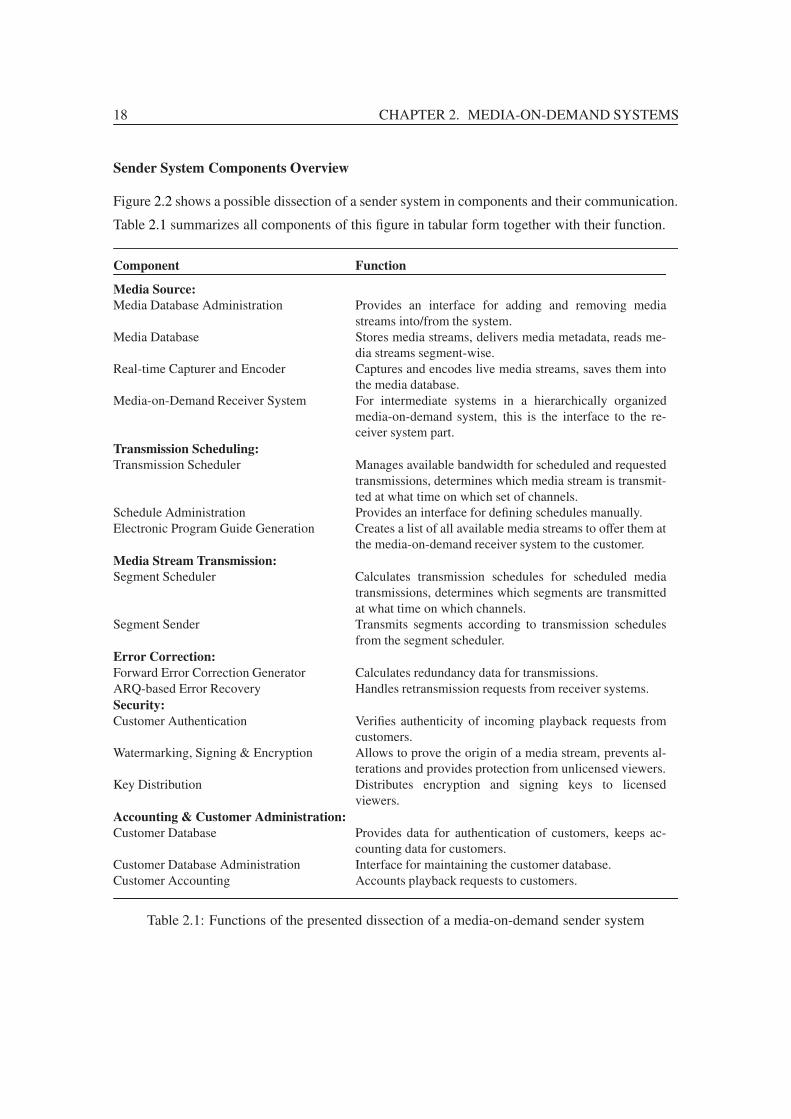
18 CHAPTER 2. MEDIA-ON-DEMAND SYSTEMS
Sender System Components Overview
Figure 2.2 shows a possible dissection of a sender system in components and their communication.
Table 2.1 summarizes all components of this figure in tabular form together with their function.
Component Function
Media Source:
Media Database Administration Provides an interface for adding and removing mediastreams into/from the system.
Media Database Stores media streams, delivers media metadata, reads me-dia streams segment-wise.
Real-time Capturer and Encoder Captures and encodes live media streams, saves them intothe media database.
Media-on-Demand Receiver System For intermediate systems in a hierarchically organizedmedia-on-demand system, this is the interface to the re-ceiver system part.
Transmission Scheduling:
Transmission Scheduler Manages available bandwidth for scheduled and requestedtransmissions, determines which media stream is transmit-ted at what time on which set of channels.
Schedule Administration Provides an interface for defining schedules manually.Electronic Program Guide Generation Creates a list of all available media streams to offer them at
the media-on-demand receiver system to the customer.Media Stream Transmission:
Segment Scheduler Calculates transmission schedules for scheduled mediatransmissions, determines which segments are transmittedat what time on which channels.
Segment Sender Transmits segments according to transmission schedulesfrom the segment scheduler.
Error Correction:
Forward Error Correction Generator Calculates redundancy data for transmissions.ARQ-based Error Recovery Handles retransmission requests from receiver systems.Security:
Customer Authentication Verifies authenticity of incoming playback requests fromcustomers.
Watermarking, Signing & Encryption Allows to prove the origin of a media stream, prevents al-terations and provides protection from unlicensed viewers.
Key Distribution Distributes encryption and signing keys to licensedviewers.
Accounting & Customer Administration:
Customer Database Provides data for authentication of customers, keeps ac-counting data for customers.
Customer Database Administration Interface for maintaining the customer database.Customer Accounting Accounts playback requests to customers.
Table 2.1: Functions of the presented dissection of a media-on-demand sender system

2.2. STRUCTURE OF MEDIA-ON-DEMAND SYSTEMS 19MediaInput
Med
ia D
atab
ase
Adm
inis
trat
ion
Sch
edul
e
Adm
inis
trat
ion
Cus
tom
er D
atab
ase
Adm
inis
trat
ion
Cus
tom
er
Aut
hent
icat
ion
Med
ia D
atab
ase
Rea
l−ti
me
Cap
ture
r &
Enco
der
Med
ia−
on−
Dem
and
Rec
eiver
Syst
em
Tra
nsm
issi
on
Sch
edule
r
Ele
ctro
nic
Pro
gra
m
Guid
e G
ener
atio
n
Seg
men
t S
ched
ule
r
Seg
men
t S
ender
Cust
om
er D
atab
ase
Cust
om
er
Acc
ounti
ng
AR
Q−
bas
ed
Err
or
Rec
over
y
Forw
ard E
rror
Corr
ecti
on
Key
Dis
trib
uti
on
Wat
erm
arkin
g
Sig
nin
g &
Encr
ypti
on
Request
Playback
Authenticated
Cust
om
er
Dat
aS
ched
ule
Dat
a
Pla
nned
Med
ia S
trea
ms
Pre
−re
cord
ed
Live Media
Stream Sender System
on−Demand
To Parent Media−
Med
ia
So
urc
e
Tra
nsm
issi
on
Sch
edu
lin
g
Cu
sto
mer
Acc
ou
nti
ng
&
Ad
min
istr
.
Sec
uri
ty
Med
iaS
trea
mT
ran
smis
sio
nE
rro
rCo
rrec
tio
n
Signing Keys
Encryption &Media Stream
Segments
Secured
Med
ia S
trea
m D
ata
Med
ia R
eques
ts
Cust
om
er D
ata
Sch
eduli
ng D
ata
Encr
ypti
on K
eys
Pro
gra
m G
uid
e
Leg
end:
Electronic
Program Guide
Fro
nte
nd
NetworktoReceiver
Fig
ure
2.2:
Adi
ssec
tion
ofa
med
ia-o
n-de
man
dse
nder
syst
em

20 CHAPTER 2. MEDIA-ON-DEMAND SYSTEMS
2.2.2 Receiver-Side Components of a Media-on-Demand System
On the receiver side, the system can be dissected in a very similar way into components:
Reception Scheduling
To start a media-on-demand reception, the customer has to select the media stream he wants to
see through the media stream selection component, probably using data from the electronic pro-
gram guide storage or information passed outside the scope of the media-on-demand system (e. g.
a printed program guide, advertisements, a permanent program guide channel, . . . ). Additionally,
the reception scheduler has to check if enough resources (e. g. bandwidth, storage) are available
for the reception of the selected media stream and reserve the required resources for the duration
of the reception.
Media Reception
When a media stream has been selected for reception, the playback scheduler has to evaluate the
transmission parameters: Each media-on-demand transmission may use a set of channels which
must be joined and left at specific times (esp. if the reception bandwidth of the media-on-demand
receiver system is limited). Additionally, several further channels may be used for optional ser-
vices (e. g. to increase the media stream quality or to add error correction redundancies). The
playback scheduler selects the channels to join and instructs the segment receiver to receive seg-
ments from the channels.
Media Destination
The segment receiver then tunes into the selected channels and forwards the received segments to
the segment storage. Depending on the type of interactivity and the used transmission scheme,
this segment storage may be very small (only a buffer for compensating jitter of the media data
transport system) up to very huge (e. g. to provide some support for playback control requests to
transmission schemes which do not support any type of interactivity by themselves).
From the segment storage, the segments are read by the media player and presented to the
consumer. For interactive media streams, the consumer can send playback control or content
navigation requests to the aforementioned reception scheduler, so it can update its schedule and
instruct the playback scheduler about the new schedule.
If the media-on-demand receiver system is an intermediate system (see section 2.3), the re-
ceiver system obtains its requests from the attached media-on-demand sender system and forwards
all received data to this system.

2.3. TOPOLOGY OF MEDIA-ON-DEMAND SYSTEMS 21
Error Correction
To compensate for lost (or corrupted) data on the media data transport system, the sender system
may have added forward error correction redundancy, support ARQ-based error recovery or
a combination thereof. The receiver system may benefit from forward error correction if it can
reconstruct lost or corrupted data with the help of the redundancy data or by requesting retrans-
missions.
Security
Analogical to the security components of the sender system, corresponding components at the
receiver side are required: If a back-channel from the receiver system to the sender system is
available, the media-on-demand sender system may require a playback request for the transmission
of the media stream. To authenticate the customer to the media-on-demand sender system, a
customer authentication component may be required. Accordingly, a decryption & signature
checking component and a key reception component are needed to decrypt the media stream or
to verify the stream integrity and to obtain the used encryption and signing keys if non-static keys
are used.
Customer Identification
To identify a customer in the media-on-demand receiver system, a customer login component
may be used.
Receiver System Components Overview
Figure 2.3 shows a dissection of a receiver system into the aforementioned components and their
communication. Table 2.2 summarizes all components of this figure in tabular form together with
their function.
2.3 Topology of Media-on-Demand Systems
Simple media-on-demand systems depict a star topology, where the center node is the sender
system and the other nodes are receiver systems (see figure 2.4a). But for large media-on-demand
installations it may be advisable to use a more complex topology where sender systems are repli-
cated for reliability, load balancing or for locality reasons.
Higher reliability can be reached if several sender systems are located within the reception area
of each receiver system. In case of a failure, other systems must be able to take over existing
transmissions of the failed system or at least serve new media requests. Similarly, to lower load
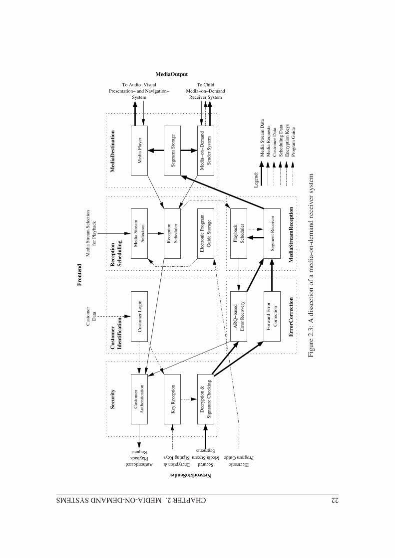
22CHAPTER2.MEDIA-ON-DEMANDSYSTEMS
MediaOutput
Cus
tom
erA
uthe
ntic
atio
nC
usto
mer
Log
in
AR
Q−
bas
ed
Err
or
Rec
over
y
Forw
ard E
rror
Corr
ecti
on
Seg
men
t R
ecei
ver
Pla
ybac
k
Sch
edule
r
Ele
ctro
nic
Pro
gra
m
Guid
e S
tora
ge
Rec
epti
on
Sch
edule
r
Med
ia S
trea
m
Sel
ecti
on
Med
ia P
layer
Seg
men
t S
tora
ge
Med
ia−
on−
Dem
and
Sen
der
Syst
em
Key
Rec
epti
on
Dec
rypti
on &
Sig
nat
ure
Chec
kin
g
Request
Playback
Authenticated Encryption &
Signing Keys
Secured
Media Stream
Segments
Electronic
Program Guide
Med
ia S
trea
m D
ata
Med
ia R
eques
ts
Cust
om
er D
ata
Sch
eduli
ng D
ata
Encr
ypti
on K
eys
Pro
gra
m G
uid
e
Leg
end:
Cust
om
er
Dat
afo
r P
laybac
k
Med
ia S
trea
m S
elec
tion
To Audio−Visual
Presentation− and Navigation−
System Receiver System
Media−on−Demand
To Child
Sec
uri
tyC
ust
om
er
Iden
tifi
cati
on
Rec
epti
on
Sch
edu
lin
g
Med
iaD
esti
na
tio
n
Err
orC
orr
ecti
on
Med
iaS
trea
mR
ecep
tio
n
Fro
nte
nd
NetworktoSender
Fig
ure
2.3:
Adi
ssec
tion
ofa
med
ia-o
n-de
man
dre
ceiv
ersy
stem

2.3. TOPOLOGY OF MEDIA-ON-DEMAND SYSTEMS 23
Component Function
Reception Scheduling:
Media Stream Selection Handles selection of a media stream to request.Electronic Program Guide Storage Keeps a list of the currently available media streams for
playback.Reception Scheduler Manages available bandwidth for scheduled and requested
receptions, determines which media stream is received atwhat time.
Media Reception:
Playback Scheduler Determines which segments have to be received until whattime on which channels.
Segment Receiver Receives segments and stores them into the segmentstorage.
Media Destination:
Segment Storage Stores media stream data segment-wise.Media Player Presents the media stream to the consumer, forwards navi-
gation requests to the playback scheduler.Media-on-Demand Sender System For intermediate systems in a hierarchically organized
media-on-demand system, this is the interface to the sendersystem part.
Error Correction:
Forward Error Correction Recovery Evaluates redundancy data for recovery of lost or corruptedsegments.
ARQ-based Error Recovery Requests retransmission for lost or corrupted segmentsfrom the sender system.
Security:
Customer Authentication Authenticates outgoing playback requests.Decryption & Signature Checking Decrypts encrypted transmissions and checks digital signa-
tures of signed transmissions.Key Reception Receives encryption and signing keys.Customer Identification:
Customer Login Accepts identification data of the customer.
Table 2.2: Functions of the presented dissection of a media-on-demand receiver system
and bandwidth usage of sender systems or of the network, requests of receiver systems can be
distributed to different sender systems, e. g. taking the current load or the distance between the
sender and receiver system into account or using a random or preset assignment.
Reducing the network distance between sender and receiver systems can have several reasons
which mostly depend on the type of the used network. One possible reason is to reduce the load
of the network: The shorter the network distance between sender and receiver, the less routers or
switches and the less data link connections are affected by the transmission. Sometimes locality is
even required due to missing routing capabilities of the underlying network (e. g. if multicasting
capabilities are required for the media stream transmission).
Besides of simply using several independent sender systems (see figure 2.4b), the sender sys-
tems can also be connected to each other. If a strict hierarchy is used for all sender systems (i. e.

24 CHAPTER 2. MEDIA-ON-DEMAND SYSTEMS
one designated sender system serves as master to all other sender systems, either directly or indi-
rectly), this leads to a tree topology (see figure 2.4c): In this tree the master sender system is
located at the root of the tree, the remaining non-leaf nodes work as intermediate sender systems
and the receiver systems are positioned at the leaf nodes.
R
R
R
R
R R
S
(a) Media-on-demand system using a star topology
S
R
S
R
R
R
R
R
RR RR
R
R
S
R
R R
R RR
(b) Several independent star topologies which serve re-ceiver systems locally
R
S
R
SR
R R
R
R
S
RR RRR RR R
S
(c) Hierarchically organized media-on-demand system using a tree-topology
Figure 2.4: Three example topologies for media-on-demand systems
Using a tree topology for organizing huge media-on-demand systems has the advantage that
maintenance is much easier: Changes to the media assortment must not be performed on every
media-on-demand sender system but only on the master sender system from where the changes are
distributed to the intermediate sender systems. When a request for a media stream is received by
an intermediate system, it can request the media stream on its parent media-on-demand system
and send the received media data to its child systems. Besides of only forwarding media streams,
intermediate systems can also cache the received media streams into their media database for
answering subsequent requests for the same media stream without involving their parent media-
on-demand system again.
But instead of using some file transfer software for transferring media streams between sender
systems, it is possible to use media-on-demand transmissions at every level in the hierarchy. This
gives two advantages: Firstly, by using media-on-demand transmissions even between sender
systems, duplicate requests from several intermediate sender systems to a common parent system
can be combined into a single transmission in the same way as duplicate requests from several

2.4. CLASSIFICATION OF MEDIA TRANSMISSION SYSTEMS 25
receiver systems to a common sender system, saving bandwidth for the transmissions between
sender systems. Secondly, when a media stream is transmitted linearly from the parent media-on-
demand system to an intermediate media-on-demand system at the time of the request from the
media-on-demand receiver system, the intermediate media-on-demand system has no immediate
access to the full media stream but just to the currently received part. This is comparable to
a live (or near-live) transmission for the intermediate media-on-demand system which results in
higher bandwidth requirements for some transmission schemes. Using the same media-on-demand
transmission scheme at every level of the topology allows the intermediate systems to just forward
the received data; no access to missing parts of the media stream is required at any time.
From another point of view, a hierarchical media-on-demand system can be regarded as an
assembly of several simple media-on-demand systems, using a star topology at each subtree in
the complete hierarchy tree: While the master sender at the root of the hierarchy serves as media-
on-demand sender system only, intermediate systems are constituted out of a media-on-demand
receiver system (for receiving media streams from their parent system) and a sender system (for
sending media streams to their child systems). The receiver systems at the leaf nodes remain
unchanged; the full topology is hidden at this level.
Several other topologies are possible, too, e. g. setups where all sender systems are connected in
a ring or constitute a complete or incomplete (perhaps even irregular) mesh and receiver systems
may be connected to one or several sender systems in rings or stars, but these setups loose most of
the above mentioned advantages of the tree topology.
2.4 Classification of Media Transmission Systems
Classification of media transmission systems is a difficult matter as there are a lot of characteristics
which can be used for a classification. Most commonly, media transmission systems are divided
into groups depending on the supported level of user interactivity, but from a provider’s point of
view many other criteria may be more important, e. g. the required communication type of the
network or the ability to transmit live streams.
In the following subsections, several classification schemes are introduced which help to bench-
mark and compare the transmission schemes which are proposed in the next chapter. For a better
overview, the given classifications are presented in two groups:
• Technical classification schemes:
This group is the larger one and includes classifications by communication type, network
type, transmission scheme and many less important ones.
• Functional classification schemes:

26 CHAPTER 2. MEDIA-ON-DEMAND SYSTEMS
This group contains classifications which concern the range of supported functions of the
transmission system, examining both capabilities for providers and for consumers.
2.4.1 Technical Classification of Media Transmission Systems
The technical classification of media-on-demand systems is a very important issue as this clas-
sification allows a provider to perform a preselection of transmission schemes which fit to her
prevailing conditions. For example, if a provider wants to use a wide-area broadcasting network
for media-on-demand (e. g. using satellites), he cannot use transmission schemes which serve
only a single customer for each transmission (or at least not cost-effective). Thus technical clas-
sifications characterize if a transmission scheme can (theoretically and practically) be used when
the technical infrastructure is preset and immotile. Otherwise, if the infrastructure has not been
specified, technical classifications can help to define the requirements.
Communication Type
One important characteristic for media-on-demand systems is the communication type: Tradi-
tional media-on-demand systems are based on one-to-one transmissions for the delivery of media
streams. As a consequence, the bandwidth and throughput requirements for media-on-demand
sender systems are proportional to the number of concurrently active media-on-demand receiver
systems.
One-to-many transmissions provide a way to lower these requirements: The media-on-demand
system sends the data once on a broadcast or multicast channel and it is up to the network protocol
to deliver the data to all active receiver systems efficiently. This way, the sender system can trans-
mit data to an arbitrary number of receiver systems without increasing the bandwidth requirements
of the sender system proportional to the number of transmissions.
It is also possible to use a combination of one-to-one and one-to-many transmissions, e. g.
sending often requested media streams using one-to-many transmissions and seldom requested
streams using one-to-one transmissions. Some transmission schemes even combine one-to-one
and one-to-many transmissions for a single transmission, e. g. a one-to-many transmission is used
for the main part and one-to-one transmissions are used for missed parts of latecomers.
Nearly any communication network can be used for media transmissions (provided that the net-
work offers a suitable bandwidth, short latency and a sufficient quality-of-service), so this section
can only give a short overview of the most commonly used network types for media-on-demand.
Broadcasting Networks: Broadcasting networks have a long history for non-interactive media
transmissions (i. e. traditional radio and TV) as they can be used to reach a huge number
of recipients at once. Plain analog over-the-air (i. e. radio wave based) transmissions have

2.4. CLASSIFICATION OF MEDIA TRANSMISSION SYSTEMS 27
been used anciently, followed by analog broadcasts over cable TV (CATV) networks, and
further followed by digital broadcasts over satellite, air, cable and cellular phone networks.
For media-on-demand, digital networks are required by nearly any of the transmission
schemes, so the digital successors (e. g. based on DVB-T, DVB-C and DVB-S) are can-
didates for media-on-demand. But also cellular phone networks (e. g. using GPRS, UMTS
or DVB-H) or short-range networks like local area networks of different type (e. g. Ethernet
or wireless LAN) can be used for media-on-demand transmissions.
All of the aforementioned networks can be used for one-to-many transmissions in media-on-
demand systems. They mainly differ in the number of recipients they can reach (satellite-
based networks can typically reach more recipients than terrestrial networks, cable TV net-
works, cellular phone networks or even local area networks).
The more recipients a sender system can reach, the higher is the availability of the provided
service. But at the same time, the more recipients are reached, the more recipients have to
share the same bandwidth. Thus, reaching a high number of recipients through broadcast-
ing is only advantageous if all recipients request the same small set of media streams. If
many different media streams are requested, several small broadcasting networks are more
beneficial.
Multicast-Capable Networks: Many networks provide a way which can be used to transmit
a media stream from one sender to several recipients without sending the data several
times over a link. The most common multicast-capable communication protocols com-
prise multicast-capable IP networks (e. g. the M-BONE, a satellite link using MPE, ULE or
GSE encapsulation to transmit IP packets or local area networks) and ATM networks. Ad-
ditionally, it is possible to setup tunnels through unicast networks to bypass non-multicast
links. If the Internet provider where the home systems are connected to (e. g. by DSL)
supports multicasting, it is even possible to provide multicast service up to the home4.
Similar to broadcasting networks, multicast-capable networks can be used for one-to-many
transmissions in media-on-demand systems.
Unicast Networks: Unfortunately, the major part of the current Internet does not provide mul-
ticast services yet. But all of the aforementioned multicast-capable networks also provide
unicast functionality, and even the broadcast networks can be used for unicast transmissions,
so all mentioned protocols can be used for one-to-one transmissions in media-on-demand
systems. But as the available bandwidth is typically the more expensive the more recipients
can be reached with it, large broadcasting networks are not cost-effective if they are used
4Unfortunately, many Internet providers do not provide multicast services to their customers yet, often not becauseof technical problems but just because of missing means for accounting multicast traffic at the sender side.

28 CHAPTER 2. MEDIA-ON-DEMAND SYSTEMS
to transmit large amounts of data to single recipients. (Chapter 6 presents a comparison of
the costs for unicast- and multicast-based media-on-demand systems in different network
setups.)
Back-Channel Support
For some media-on-demand transmission systems it is necessary that requests for media streams
are transferred from the media-on-demand receiver system to the sender system. These systems
are called reactive, online, close-loop or user-centered. The counterpart of these systems, the
pro-active, offline, open-loop or data-centered media-on-demand systems, perform permanent
broadcasts, independent of any signaling of receiver systems.
Both types of systems have their own advantages: A reactive system can provide immediate
service and can omit unnecessary transmissions because it has knowledge about active recipients
of ongoing transmissions. Additionally, a reactive system can provide a much higher type of
interactivity (up to virtual reality, see section 2.4.2). Accounting (e. g. pay-per-view), encryption
(e. g. using keys which are only announced to active recipients) and error correction (e. g. using a
NACK-based mechanism) benefit from a back-channel, too.
But pro-active systems have the advantage that they provide a better scalability in huge sys-
tems: As a pro-active system does not get any feedback from the receiver systems, their operation
is not influenced by the number of active receiver systems. Esp., pro-active systems always pro-
vide the same quality of service: The playback delay will always be determined by the provider
when scheduling the media stream transmission, it will never be the case that the playback delay
increases because the media transport system is overloaded from too many active recipients. Last
but not least, pro-active systems do not require a back-channel, so they can even be used if the
transport system only provides a unidirectional service.
To benefit from several of the advantages of both types, reactive-pro-active hybrid systems
combine mechanisms from both sides, so they can provide immediate service, a better scalability
and a bandwidth reduction at the same time.
Topology of Media Transmission Systems
The media content in a media transmission system can travel on different ways, but in total it
is transferred from a single or limited number of sender systems to a huge number of receiver
systems. As stated in section 2.3, several topologies are possible, e. g. stars, trees or any type of
meshes.
The advantage of using complex topologies instead of a simple star topology is to limit the
number of playbacks of each sender system so the load and bandwidth use can be lowered. Another
advantage is increased robustness to failures of sender systems if other sender systems can take

2.4. CLASSIFICATION OF MEDIA TRANSMISSION SYSTEMS 29
over the tasks of failed systems. The disadvantage of using multiple, possibly distributed sender
systems are higher installation and maintenance costs.
Besides of utilization and failover reasons, the use of complex topologies depends as well
on the type of the network: For example, if the media stream is transmitted via satellite with all
receiver systems in the satellite footprint, complex topologies do not make any sense as all receiver
systems share the same data link between sender and receiver systems, but for large media-on-
demand systems using point-to-point connections or routing multicast connections, hierarchies or
meshes are very beneficial.
In some cases, even both ways are possible: For example for cable TV networks, the band-
width of the network will be most probably the limiting factor which determines the number of
concurrently active media streams, so if only a few, popular media streams should be transmitted,
no hierarchies are needed. At the other extreme, if the media assortment is very large and does not
contain many popular media streams, placing one intermediate sender system at each cable TV
network segment feed allows to transmit the same number of concurrently active media streams at
each segment as before in the whole setup.
Another problem of retrieving a media stream through a chain of sender systems (e. g. along
the path from the master sender system through intermediate sender systems to the receiver sys-
tem in case of a tree topology) occurs at the intermediate sender systems: When media streams
are transmitted to intermediate sender systems as a result of a request from a receiver system, the
intermediate sender system has no access to the whole media stream during the transmission but
only to the yet received parts. This is a situation similar to the live streaming problem (see sec-
tion 4.17) where the sender system cannot access future parts of the media stream for transmission.
Fortunately, one advantage over live streaming exists: If the intermediate sender system uses the
same transmission scheme as its parent system, the received data can simply be forwarded without
caring for live streaming issues because the parent sender system already guarantees that all data
will be available in due time.
Bandwidth Requirements
The bandwidth requirements at the sender side and at the receiver side depend on many parameters.
For the media-on-demand sender system, the following parameters may influence the bandwidth
requirements:
• The number of transmitted media streams,
• the number and join times of receiver systems receiving a media stream,
• the number and bandwidth of the channels used for the transmissions (which may in turn
depend on the transmission parameters, e. g. the playback delay),

30 CHAPTER 2. MEDIA-ON-DEMAND SYSTEMS
• the amount of bandwidth which is needed for preloading (see section 3.5.4 and 4.6).
For the receiver system, only the following parameters are of interest:
• the number and bandwidth of the channels used for the transmissions,
• the amount of bandwidth which is needed for preloading.
To describe the bandwidth requirements of a transmission scheme, it is sensible to describe the
sender and receiver bandwidth requirements in multiples of the media stream bit rates and to
mention if it is possible to adapt the transmission scheme to a specific receiver system bandwidth
(probably with impacts to other parameters, e. g. the sender system bandwidth requirements or the
playback delay).
Storage System Requirements
The size requirements of the storage system at the sender side are very obvious: The media-on-
demand sender system must be able to keep all media streams of the offered media assortment into
its media database. The throughput of this storage system equals the sender system bandwidth
(ignoring the fact that parts of the media stream may reside in the file system cache if they are
transmitted twice within short time).
Unfortunately, size and throughput are not the only requirements to the storage system: If the
sender system is sending a lot of media streams (or a lot of segments of a single media stream) at
the same time, the storage system must be able to perform this many direct accesses to the media
streams. For systems using hard disks, this requires a lot of seek operations which slows down the
throughput of the storage system. If we assume a fixed amount of memory for read-ahead for a
whole media stream transmission, the only value which influences the seek rate is the number of
media stream positions from which data is read in parallel during the transmission:
One position per channel: The media stream data is read from one position for each transmitted
channel.
One position per slot: The media stream data is read from several positions for each transmitted
channel, but only from one position for each slot on the channel.
Multiple positions per slot: The media stream data is read from several positions for each trans-
mitted channel, even for each slot on the channel.
The size requirements of the storage system at the receiver side depend on several parameters:
• The size of the received media streams,
• the amount of the media stream which must be buffered (which depends on the used trans-
mission scheme),

2.4. CLASSIFICATION OF MEDIA TRANSMISSION SYSTEMS 31
• the time the received media streams should be available after reception,
• the amount of storage which is needed by preloading.
For the classification of the receiver system storage requirements, we use the following classes:
No media stream buffering: The receiver system does not store any media stream data except
for jitter compensation.
Partial media stream buffering: The receiver system must buffer part of the media stream.
Configurable media stream buffering: The receiver system must buffer part of the media
stream, the amount can be configured freely (but may influence other parameters, e. g. the
sender bandwidth requirements)
Full media stream buffering: The receiver system must buffer the whole media stream.
Partial media stream buffering and partial preloading: The receiver system must buffer part
of the media stream and additionally the beginning of several/all media streams of the media
assortment.
Configurable media stream buffering and partial preloading: The receiver system must
buffer part of the media stream, the amount can be configured freely; additionally the
beginning of several/all media streams of the media assortment must be stored.
Full preloading: The receiver system must buffer all media streams of the media assortment.
The throughput of the receiver storage system equals the receiver system bandwidth plus the bit
rate of the played media streams (again ignoring the file system cache).
Similar to the sender system, direct access operations are required for storing all received seg-
ments of each media stream (either when receiving them or when assembling them for playback).
The seek rate of the receiver system can then be classified as:
One position per channel: The media stream data is written to one position for each received
channel.
One position per slot: The media stream data is written to several positions for each received
channel, but only from one position for each slot on the channel.
Multiple positions per slot: The media stream data is written to several positions for each re-
ceived channel, even for each slot on the channel.
Some transmission schemes do not require any data to be stored, but on the other side, they
require a high sender system bandwidth. Other transmission schemes concentrate on lowering the
sender system requirements but have high receiver system requirements and storage requirements.
In general, storage and bandwidth requirements of sender and receiver are contrary parameters of a

32 CHAPTER 2. MEDIA-ON-DEMAND SYSTEMS
media-on-demand transmission scheme and it is not possible to keep them all low at the same time.
An ideal media-on-demand transmission scheme should therefore be adjustable in the parameters
to find the right compromise between these parameters.
2.4.2 Functional Classification for Media Transmission Systems
In this section, several classifications are introduced which can be used to grade a media trans-
mission system. While the technical classifications of the last section are almost only relevant
for providers, most of the functional classifications are interesting for the consumer, too, as these
classifications specify the capabilities of the media transmission system.
Media Scheduling
Requesting a media playback can be as simple as tuning into an ongoing transmission, but often a
more complex procedure is required, e. g. sending a request to a remote system and negotiating the
playback. Throughout this thesis, the following terms are used for describing the different classes
for media scheduling:
Prearranged: The media transmissions are scheduled to fixed dates. No request processing from
client systems is possible; the media transmission has to be joined at the scheduled trans-
mission time to be received.
Pro-active media-on-demand: The media transmission is performed permanently. No request
processing from client system is required; the media transmission can be joined at any time
(probably with a reasonable playback delay).
Reactive media-on-demand: The media transmission is performed on demand. The media trans-
mission can be joined only after a request has been issued (possibly with a reasonable play-
back delay).
Combinations: For example, the media transmission can be joined at any time when a long play-
back delay is accepted, but by sending a request, an additional transmission is scheduled.
Other combinations (e. g. combining prearranged with reactive media-on-demand) are also
possible.
Interactivity Levels of Media Transmission Systems
In [GKSW91], the authors classified media-on-demand and interactive TV services by their level
of interactivity into the following five categories:
Broadcast (No-VoD): No interactive control.
Pay-per-view (PPV): Viewer signs up for specific programming.
2.4. CLASSIFICATION OF MEDIA TRANSMISSION SYSTEMS 33
Quasi video-on-demand (Q-VoD): Users are grouped based on a threshold of inter-
est, users can switch to a different group.
Near video-on-demand (N-VoD): Limited interactive control, e. g. rewind and fast
forward in steps of 5 minutes.
True video-on-demand (T-VoD): Full control over playback.
Although this classification allows a simple classification of media-on-demand and interactive
TV services of the early nineties, it brings several drawbacks and limitations when classifying
today’s media-on-demand services:
• Different types of classification are mixed together, e. g. communication type (broad-
cast), accounting type (pay-per-view), media scheduling (on-demand) and playback control
(rewind, fast forward).
• The selected classes only represented the available types of media-on-demand/interactive
TV services of the late eighties/early nineties (e. g. quasi video-on-demand describes Batch-
ing transmissions (see 3.3.2) and near video-on-demand describes channel changes of Stag-
gered transmissions (see 3.4.2)). Later developments cannot be assigned to any of these
classes (e. g. it is not possible to find a class for a transmission scheme which delivers a
media on request with a short delay but allows nearly no other type of interactivity which is
common for pro-active transmission schemes).
• The classes do not allow a precise specification of the possible types of interactivity. For
example, a class where the user can pause or rewind the playback but cannot use fast forward
is not given.
• The used terms unnecessarily cause the impression that the transmission system can only be
used for one type of media content (video).
For a better classification of the media-on-demand schemes, a more fine-grained classification
of interactivity is beneficial. Because of the huge breadth of different types of interactivity, the
interactivity classification is split into two distinct classes5:
Playback Control: Playback control means the navigation on the media stream in a VCR-like
manner, e. g. pause, fast forward, rewind, slow motion, etc., but also jumping to a scene in
the past or future of the media stream. To specify a playback control class completely, one
normally would have to enumerate all types of possible playback control. Fortunately, the
support for different types of playback controls are not unrelated to each other in media-on-
demand transmission schemes, so only the following few classes are of interest:
5The other aspects of the quoted classification — communication type, back-channel support and accounting type— are presented separately.

34 CHAPTER 2. MEDIA-ON-DEMAND SYSTEMS
No playback control: No playback control is supported.
Fixed jump playback control: No playback control is supported except for jumping for-
ward or backward for a large, fixed amount and pausing for a long, fixed time.
Playback control within received part: All types of playback control which navigate
within the transmitted part of the media are supported. This includes pause, slow
motion and rewind, but also fast forward up to the point of the initial transmission.
Jumping to specific locations in the media (either specified by time or chapter) and
search forward and backward are possible, too (with the same restriction as for fast
forward). This is the maximum possible level of playback control for a live transmis-
sion and typically the maximum possible level of playback control for pro-active and
prearranged transmissions. (Today’s digital video recorders often support this kind of
interactivity as part of the time shifting features.)
Full playback control: All playback controls can be used, including jumping to specific
locations (e. g. using an index of scenes or selecting a specific chapter by number or
time) in past and future parts of the media stream.
The level of playback control can always be raised up to rewind interactivity if the receiver
system has the ability to store the whole received part of the media stream while it is received
at single playback rate.
Content Navigation: Content navigation can be distinguished from playback control by the type
of interaction: While playback control only influences the speed of the playback and rep-
etitions of it, content navigation changes the displayed content of the media stream itself.
For example, playback control requests can be used to see the ending of a movie at the be-
ginning of the playback, but content navigation requests can be used to select an alternative
ending for the movie. In this sense one can regard playback control as a way to navigate on
continuous media streams while content navigation is used for non-continuous navigation
(see also section 2.5.1 for a detailed description of the media content structure). Within this
thesis, the following classification for content navigation is used:
No non-continuous navigation: No content navigation is supported.
Branch navigation: If the media stream contains branches (e. g. alternative scenes, view
angles), the consumer is able to choose which fork she wants to follow.
Multi-branch navigation: If the media stream contains branches, the consumer is able to
switch between the branches at any time or display several branches at once (“Picture-
in-Picture”).
Full content navigation: Any type of content navigation is possible (e. g. virtual reality).
2.4. CLASSIFICATION OF MEDIA TRANSMISSION SYSTEMS 35
Many other types of content navigation are conceivable (e. g. accessing extra information,
change of language, interactive shopping, interactive advertisements, navigating between different
media streams [LV93]) but they can be reduced to the above given list of interactivities (e. g.
access to extra information can be viewed as a branch in the media), a combination from the
reception of several media streams (e. g. if one audio stream per language and one video stream
are transmitted in parallel, a change of the language is simply a change of the audio stream) or to
activities which do not influence the design of a media-on-demand transmission schemes (e. g. if
payment information have to be transmitted for interactive shopping).
Dynamic Schedule Changes
For pro-active transmissions, the provider has to decide which media streams she wants to transmit
and divide the available bandwidth to these transmissions. Therefore, the provider has to configure
a bunch of properties which influence the bandwidth of a transmission, e. g. the media stream
encoding and bit rate, the transmission scheme to use, the maximum tolerated playback delay and
the amount of added redundancy for error correction.
For many of these decisions, the provider does not want to tie himself down to fixed values. For
example, the popularity of media streams may depend on the daytime, the day of week, special
events or even the weather. The flexibility and dynamic adaptability of the used transmission
scheme is therefore described by the dynamic scheduling classification:
No dynamic change support: None of the parameters of a transmission can be changed dynam-
ically.
Dynamic bandwidth and playback delay change support: The bandwidth and the playback
delay can be changed dynamically. Typically, bandwidth and playback delay are opposi-
tional parameters, i. e. the bandwidth increases when the playback delay is decreased and
vice versa.
Dynamic stream duration prolongation: For live transmissions, the total media stream duration
may be unknown in advance, thus it may be necessary to keep the media stream duration
dynamic.
Dynamic content support: For some transmissions, it may be useful to exchange the content of
the transmission dynamically: For example in a news transmission, single contributions may
be replaced by newer ones.
Depending on the transmission scheme, these changes may come into effect immediately or after
some delay. Furthermore the impact of dynamic changes may differ as some transmission schemes
perform less efficient if dynamic changes are used or even made possible.

36 CHAPTER 2. MEDIA-ON-DEMAND SYSTEMS
Variable-Bit-Rate Media Support
When a media stream is to be encoded, the producer has great latitude how to encode the media
stream: Besides of selecting a media format (see section 2.5.3), it is often possible to select the
encoding quality of the resulting media stream. Typically, the encoding quality is determined by
configuring a target bit rate.
Many media formats use lossy encodings which remove some of the highest details when the
target bit rate is too low. These media formats often allow two different configurations:
Constant-bit-rate (CBR): The media stream has a (nearly) constant bit rate.
Variable-bit-rate (VBR): The bit rate of the media stream varies over time.
Although the variable-bit-rate encoding provides the higher quality of these two (for the same
average bit rate), it is not supported by every transmission scheme. In this case smoothing to
constant-bit-rate (see section 4.8) can be utilized as a bypass.
Live Streaming Capability
Live streaming means the capability to transmit a media stream which is just captured and encoded.
The reason why live streaming is mentioned for classification is that live transmissions impose
several problems to the transmission scheme: Many of the transmission schemes assume that the
media stream is completely known and available at media startup, but for live transmissions this is
not true:
• The duration of a live transmission may be unknown.
• The media content is not known in advance, only the yet captured and encoded part of the
media stream is accessible, which disallows the transmission of later parts of the media
stream.
• Any additional information about the media stream is unknown for the remaining part, e. g.
the time, duration and strength of bandwidth variations of a variable-bit-rate media stream
are unpredictable.
While the first item objects the dynamic stream duration prolongation capability which has
already been mentioned above, the latter ones require a further classification:
Not live streaming capable: The transmission scheme does not support live streaming at all.
CBR live streaming capable: The transmission scheme supports only live streaming of constant-
bit-rate media streams.
Full live streaming capable: The transmission scheme supports live streaming of CBR and VBR
media streams.

2.5. MEDIA CONTENT AND FORMAT 37
Similarly to live streaming, near-live streaming means the capability to transmit a media stream
with a short delay after capture. As near-live streaming does not lower the requirements of live
streaming to the media transmission system significantly no further classification is introduced
for near-live streaming. The main advantage of near-live streaming to real live streaming is an
improved result for smoothing of bandwidth variations.
Accounting Type
Financing of media-on-demand services is possible in different ways:
Free access: The service may be accessible for no charge. This may apply if the service is state-
subsidized or financed through commercials.
Pay-per-view: The consumer has to pay for each requested media stream transmission.
Pay-per-subscription: The consumer pays regular fees for the media streams of a media stream
set.
Combinations: Any type of combination is possible, too: For example, a pay-per-view system
with additional regular fees or a service where the consumer can select between advertising
sponsored transmissions and paid, ad-free ones.
Besides of the requirement of a back-channel for pay-per-view and of access restrictions (e. g.
using encryption) for non-free access, these accounting types have no effects on media-on-demand
transmissions and are not examined in this thesis.
2.5 Media Content and Format
The most important value for media-on-demand systems is the media itself. The media content
may be as simple as a continuous video stream but also as complex as any graph-structured, piece-
wise continuous, real-time data collection, containing alternative endings, different view angles,
selectable languages and subtitles, breaks for commercials, dynamically updated parts, etc. The
first subsection of this section gives an overview of the different structures for media content of
media-on-demand systems.
Media streams can carry different content types of media, e. g. movies, news, or radio plays,
and can use a manifold of different encodings. In subsections 2.5.2 and 2.5.3, several media types
and encodings are presented, resp., and their structure is analyzed. Additionally, properties like
variable-bit-rate and fault tolerance are reviewed.

38 CHAPTER 2. MEDIA-ON-DEMAND SYSTEMS
2.5.1 Structure of Media Content
The basic structure for the content of a media-on-demand system is a real-time data stream. The
term “real-time” herein means that a timing constraint exists: If the media content is split into
small pieces, it is possible to assign time stamps to each of them, which describe the time offset
relative to the beginning of the playback when the respective pieces are needed at the receiver
system6. The term “data stream” indicates that the media stream must have a continuous structure,
i. e. that the time stamps of the pieces are monotonously increasing.
Although the continuous structure is typical for media-on-demand content, this requirement
can be loosened: A reactive system which handles each receiver system separately can support any
type of media structure (including virtual reality). But even for pro-active systems, it is possible
to loosen the continuity requirement:
To support piecewise continuous real-time data streams, every continuous piece can be thought
of as a separate transmission, using a playback delay equal to the first possible playback time of
the piece7 after the media playback has been started (see figure 2.5 for an example).
Delay
2
D2
AB
C D1 1
AlternativeEndings
DifferentView Angles
Playback
B
(a) Example of a piecewise continuous media stream
2
A
B
B
C
D
D
1
2
1
(b) Decomposition into several continuous mediastream transmissions
Figure 2.5: Example for decomposition of a piecewise continuous media stream
Allowing piecewise continuous real-time data streams, it is possible to support all real-time
media data where the continuous pieces can be arranged as edges of a directed graph. This allows
handling the following media structures:
• Branches
• Joins
• Alternatives
• Insertions
6Exactly, it is possible to state that every data transmission has a real-time requirement which matches this definitionby stating that the whole file is needed at some time after the download has been started. Consequently, a good media-on-demand transmission scheme would find the same method for transmitting files as used in content distributionsystems: Depending on the type of connectivity either point-to-point transmission (via one-to-one connections) ora round-robin broadcast (via one-to-many connections). This way a media-on-demand system can be regarded as ageneralization of content distribution systems.
7Depending on the transmission protocol it may be possible to combine these separate transmissions into a single,comprehensive one.

2.5. MEDIA CONTENT AND FORMAT 39
Even loops are possible this way (but very uncommon).
Beneath the static structure of the media stream, the content may also change dynamically: The
simplest change is the replacement of one media stream by another (e. g. substitution of a news
transmission by an updated recording), but replacing only parts of a media are possible, too (e. g.
updating individual contributions in a news transmission).
2.5.2 Content of Media Streams
When regarding the media stream content instead of its structure, several commonly used types
can be found:
• Video streams (movies, news, . . . ): The mostly used media content type for media-on-
demand systems will be video streams8. The video stream may be as simple as a continuous
stream (as it is contained on video cassettes) but piecewise continuous stream features that
are known from DVDs can be supported, too, like
– alternative endings (branches)
– alternative beginnings (joins)
– different view angles (alternatives)
– director’s comments, deleted scenes (insertions)
• Audio streams (music, radio plays, news, . . . ): Audio streams behave very similar to video
streams, but have a much lower bandwidth; therefore the bandwidth requirements are much
lower for audio-on-demand than for video-on-demand.
• Text streams (books, tickers, subtitles): Except for subtitles to a video stream, text streams
are very uncommon for media-on-demand transmissions: Although they are normally con-
tinuous streams, a real-time requirement is very artificial (due to different and varying speed
of readers). Another issue is that pure text is very compact (a typical reader will read at most
some tens of characters per second) and only few large texts will be read without interrup-
tion, so downloading the text entirely (using either pull or push technology) probably gives
nearly the same result with much less effort.
2.5.3 Media Encodings
Because of the high bit rates of typical media streams (esp. of video streams), media-on-demand
systems utilize media compression to reduce bandwidth requirements. Media compression can
8According to the common usage, the term “video stream” hereby means an “audio-visual stream”.

40 CHAPTER 2. MEDIA-ON-DEMAND SYSTEMS
work in two ways, utilizing spatial and temporal redundancies, e. g. in case of video compres-
sion, similarities within a frame (spatial) or between frames (temporal) are registered and en-
coded. Although removal of redundancies allows creating lossless media compression schemes,
nearly all media compression schemes generally work lossy, i. e. some information is lost through
compression and cannot be retained from the compressed media stream at decompression time.
Fortunately, human senses are too imprecise and inert to recognize many of these changes as long
as only details are affected. Many media compression schemes are even specialized to human
recognition to improve the compression ratio without lowering the recognizable quality.
From the point of cost-effectiveness, the media encoding has to be selected very carefully: A
higher compression ratio reduces the required bandwidth at the media-on-demand sender system
and therefore reduces the costs for transmissions or increases the possible number of concur-
rently active playbacks. A higher compression ratio also lowers the bandwidth requirements of
the receiver system, reducing the hardware and connectivity requirements for media-on-demand
receiver systems. On the other side, high compression rates require more complex encoding hard-
ware at the sender system (which may get more relevance in case of live transmissions) and decod-
ing hardware at the receiver system, which conversely increases the costs for media-on-demand
systems.
Today, MPEG-2 [Itu00] decoder chips are very cheap (as they are produced in huge
amounts for DVB receiver systems and DVD players) and MPEG-4/Part 2 [Itu04] and
H.264/MPEG-4 AVC [Itu05b] decoder chips are available for reasonable prices today, too9.
But not only is the total bit rate of the media stream of interest: One other important issue
is the varying of the bit rate. Some media encoders produce a media stream at constant-bit-rate,
which can be handled by all media-on-demand transmission schemes, but if a variable-bit-rate
encoding is used, a higher quality can be obtained for the same average bit rate. Unfortunately,
not all transmission schemes support VBR media streams, so it is necessary to smooth the media
stream bit rate variations in these cases, loosing a lot of efficiency (see section 4.8).
Another problem is fault tolerance of the media encoding: Even if some type of error correction
is used, it is not possible to prevent losses completely (without blocking the playback for an
indefinite time). As a consequence only encodings should be used which can handle losses within
the media stream by re-synchronizing at the next logical boundary (e. g. frame or group-of-pictures
in case of video data).
9For example, Sigma Designs offers a chip which supports VC-1, WMV9, H.264/MPEG-4 AVC besides MPEG-2and MPEG-4/Part 2 as well as a wide range of audio formats (including Dolby Digital, WMA, WMA Pro, AACand MP3), encryption (including AES, DES, Triple-DES, RC4, CSS, DVB-CSA and Multi-2) and many interfaces(Ethernet 10/100, USB 2.0, IDE, PCI) [Sig06].

2.6. SUMMARY 41
2.6 Summary
This chapter provided a deep insight look into the general functioning of media-on-demand sys-
tems: Firstly, many terms related to media-on-demand have been defined and explained, the struc-
ture of media-on-demand sender and receiver systems has been shown and commented on by de-
composing them into functional units and the creation of hierarchical media-on-demand systems
has been proposed as a first, structural enhancement.
Secondly, several classifications have been proposed for media-on-demand systems. Many of
them, esp. the technical ones, determine if a specific type of media-on-demand system can be
used in a prevailing setup or which changes are required, e. g. the communication type, while the
functional classifications can be used to differentiate the provided service and utilizability of a
media-on-demand system.
Finally, the structure and content of media streams have been analyzed and properties of en-
codings have been outlined.
In the next chapter, the functioning of different types of media-on-demand systems will be
analyzed and compared to each other, using the classifications introduced in this chapter to char-
acterize the functional and technical attributes of each system.


Chapter 3
Media Transmission Schemes
IN the previous chapter, an introduction to media transmission systems has been presented,
covering the structure and operation of sender and receiver systems, an analysis of content
types and encodings of transmitted media streams and an examination of different network types
which can be used for media transmissions. This chapter focuses on one single (but important)
part of a media transmission system: the media transmission scheme.
The media transmission scheme of a media transmission system describes how a media stream
is transferred from a sender system to receiver systems. Currently, a wide range of transmission
schemes have been proposed, and the goal of this chapter is to provide an overview about their
functioning and basic approaches, their differences and commonalities and their advantages and
drawbacks.
The main goal thereby is not to present a detailed and complete description of every transmis-
sion scheme but to show the basic idea behind each of them. This understanding of the differences
between the schemes is particularly important to comprehend the evaluation and comparison pro-
cess of the transmission schemes which concludes each of the sections describing transmission
schemes.
For a further description, the classes which have been introduced in the section 2.4 are used
to classify each presented transmission scheme. Therefore, a classification table follows each
presented transmission scheme, containing the following entries:
• Technical classifications (see section 2.4.1 for a detailed description):
Communication type: The communication type which is used by the transmission
scheme.
Back-channel: Indication if a back-channel is required by the transmission scheme.
Media-on-demand topology: Topology of a media-on-demand system using this transmis-
sion scheme.

44 CHAPTER 3. MEDIA TRANSMISSION SCHEMES
Sender bandwidth: Amount of bandwidth needed at the sender system when sending a
media stream using this transmission scheme.
Receiver bandwidth: Amount of bandwidth needed at the receiver system when receiving
a media stream using this transmission scheme.
Receiver storage size: Amount of storage needed at the receiver system when receiving a
media stream using this transmission scheme.
Sender storage seeks: Amount of storage seeks needed at the sender system when sending
a media stream using this transmission scheme.
Receiver storage seeks: Amount of storage seeks needed at the receiver system when re-
ceiving a media stream using this transmission scheme.
• Functional classifications (see section 2.4.2 for a detailed description):
Media scheduling: Type of scheduling of media streams for this transmission scheme.
Playback control: Types of playback control natively supported by this transmission
scheme.
Content navigation: Types of content navigation natively supported by this transmission
scheme.
Dynamic schedule changes: Indication if changes to the schedule for ongoing transmis-
sions are possible.
Dynamic content changes: Indication if changes to the content for ongoing transmissions
are possible.
Variable-bit-rate media support: Indication if the transmission scheme supports variable-
bit-rate media streams without smoothing to constant-bit-rate.
Live streaming capability: Indication if the transmission scheme allows live (or near-live)
transmissions.
Important entries (signalling restrictions or extensions) are marked with an exclamation mark (!)
at the left, entries with mark severe restrictions with three exclamation marks (!!!).
Besides the textual (and sometimes mathematically supported) descriptions, diagrams are com-
monly added for better understanding, showing the internal structure of the transmission scheme
or presenting an example transmission in a graphical notation. The used diagram types are intro-
duced in the subsections where they are used for the first time, in particular
• channel-oriented diagrams in section 3.3.1 on page 58,
• stream-oriented diagrams in section 3.3.3 on page 63,
• enumerating transmission schedules in section 3.7.2 on page 114,
3.1. EFFICIENCY OF MEDIA TRANSMISSION SCHEMES 45
• tabular transmission schedules in section 3.7.2 on page 116,
• rectangular transmission schedules in section 3.7.2 on page 115,
• tree transmission schedules in section 3.7.2 on page 116.
Before starting with the presentation of existing transmission schemes, the following sec-
tion 3.1 provides the mathematical background for an efficiency analysis of the required band-
width of the schemes which is used to rate the schemes. In the six sections following this one,
many different schemes are presented:
Starting with some traditional media transmission schemes in section 3.2, this chapter contin-
ues with a group of reactive media-on-demand transmission schemes in section 3.3 and strides
ahead to the — most interesting — pro-active media-on-demand transmission schemes, which
are presented in sections 3.4 to 3.7. Finally, section 3.8 presents the last group of transmission
schemes which combine reactive and pro-active approaches.
In the last section of this chapter, a short summary and overall comparison of the presented
transmission schemes and enhancements is given.
3.1 Efficiency of Media Transmission Schemes
Each of the following sections concludes with a comparison of the proposed transmission schemes.
The most important issue for a comparison of different schemes is the transmission efficiency,
i. e. the bandwidth consumption for a specific setup (e. g. the required sender bandwidth for a given
maximum playback delay in case of pro-active schemes or for a given maximum playback delay
and for a specific client request pattern in case of reactive schemes) compared to the theoretical
lower limit of bandwidth which is needed to serve the same setup.
Bandwidth requirements of a transmission scheme depend very much on the prevailing condi-
tions: While the media bit rate influences the transmission bandwidth requirements linearly and
thus can be ignored in an analysis of the transmission scheme, the efficiency of a particular trans-
mission scheme is mainly influenced by parameters like playback delay and the request pattern.
For these reasons, typical request patterns for media-on-demand transmissions are examined in
the next subsection.
For a comparison of transmission schemes, an efficiency value is used which can be visualized
for different preconditions in charts at the end of each following section. This efficiency value η is
calculated by
η =B−
B(3.1)
where B is the average bandwidth consumption of the transmission scheme and B− is the mini-
mum required bandwidth for the same setup.

46 CHAPTER 3. MEDIA TRANSMISSION SCHEMES
As B ≥ B− > 0 is always fulfilled, the resulting value range of the efficiency is 0 < η ≤ 1,
where η = 1 means a perfect transmission scheme in respect to its average bandwidth consumption.
This comparison introduces a question which has first been formulated in [EVZ99a] for reactive
transmission schemes and in [ES01] for pro-active schemes: What is the minimum required band-
width to serve all requests of a given media-on-demand setup? In subsections 3.1.2 and 3.1.3, this
question is discussed and solutions for different preconditions and types of transmission schemes
are presented.
3.1.1 Request Pattern for Media-on-Demand Transmissions
The minimum required bandwidth of reactive media-on-demand transmissions is strongly influ-
enced by the request pattern for the media streams. As requests for media-on-demand transmis-
sions are in mostly any case not predictable, random processes have to be used when evaluating
transmission schemes mathematically. When request patterns for media streams are analyzed,
typically two probability distributions have to be examined:
The first distribution describes how customers’ requests are spread over the provider’s media
assortment. This distribution depends very much from the topicality and popularity of the media
streams as well as from advertisements or sales discounts, but also from time, date, season, weather
or competitive offers [LV93].
Interestingly, if the probabilities are not artificially impaired too much by the provider, the
distribution is nearly identical in mostly any case: Media streams in media-on-demand systems
are requested approximately according to the Zipf distribution with a parameter s≈ 0.729 [DPK94,
DSS94] where the Zipf distribution is defined through the probability function [KRB06a, Wik08f]
Ps[X = n] =n−s
N∑i=1
i−s(3.2)
In this formula, X is the variable of the random process, N is the total number of media streams in
the media assortment, 1 ≤ n ≤N is the rank of the examined media stream and s is the parameter
of the distribution. The resulting distribution is shown in figure 3.1 for different numbers of media
streams.
In the context of media-on-demand, the most important fact about this distribution is that most
requests are performed for a very low number of media streams: For example in case of an assort-
ment consisting of 1 000 media streams, about 36.2 % of all requests are sent for the most popular
5 % of the streams. Table 3.1 gives further examples for this distribution.
The other distribution of relevance describes how requests for a single media stream are dis-
tributed along time. Although the request rate for a single media stream varies over time (which

3.1. EFFICIENCY OF MEDIA TRANSMISSION SCHEMES 47
0
0.02
0.04
0.06
0.08
0.1
1 5 10 15 20 25
Req
uest
pro
babi
lity
Rank of media stream
Zipf distribution (N=100)Zipf distribution (N=200)Zipf distribution (N=500)
Zipf distribution (N=1000)
Figure 3.1: Zipf distribution with parameter 0.729 for media stream popularity
Number of Fraction of Fraction ofrequested media streams requested media streams requests
1 0.1% 4.8%2 0.2% 7.6%5 0.5% 13.1%
10 1.0% 18.4%20 2.0% 25.1%50 5.0% 36.2%
100 10.0% 46.7%200 20.0% 59.4%500 50.0% 80.3%
Table 3.1: Request frequencies for the most popular parts of the media stream assortment for aassortment of 1 000 media streams
may even change the popularity ranking of the media stream and shows up in the Zipf distribu-
tion), short term observations show that requests are Poisson distributed, a result which shows a
high independence of request times of different customers1.
The Poisson distribution [KRB06b, Wik08d] is parameterized by a single parameter λ and is
1Other distributions may occur if the transmission is time-bounded, e. g. most people would join the eight o’clocknews at the same time for custom reasons or join a football transmission with curiosity nearly without delay.

48 CHAPTER 3. MEDIA TRANSMISSION SCHEMES
defined by the following probability function
Pλ[X = n] =λn · e−λ
n!(3.3)
where X is again the variable of the random process, n is the number of requests during a prede-
fined period and e is the base of the natural logarithm (e ≈ 2.718281828). Figure 3.2 shows some
examples for Poisson distributions using different parameters.
0
0.02
0.04
0.06
0.08
0.1
0.12
0.14
0 20 40 60 80 100 120 140
Pro
babi
lity
Number of requests during one media stream duration
Poisson distribution (λ=10)Poisson distribution (λ=20)Poisson distribution (λ=50)
Poisson distribution (λ=100)
Figure 3.2: Poisson distribution for media stream requests
3.1.2 Minimum Required Bandwidth for Reactive Transmission Schemes
For reactive transmission schemes and a limited receiver bandwidth of R times the (constant2)
media bit rate b, the authors of [EVZ99a, EVZ01] presented the following formula assuming
Poisson distributed requests of parameter λ:
B− ≈ b · ηR · ln
(1+
λ ·dηR
)(3.4)
2Bandwidth variations are typically ignored when calculating the bandwidth requirements of a particular transmis-sion scheme. See section 4.8 for impacts of variable-bit-rate media streams to transmission schemes and the efficiencyloss which has to be expected when the transmission scheme does not support variable-bit-rate media streams natively.

3.1. EFFICIENCY OF MEDIA TRANSMISSION SCHEMES 49
where ηR is the positive real constant which satisfies the following equation:
ηR ·(
1−(
ηR
ηR+1
)R)
= 1 (3.5)
This formula has been obtained by assuming that infinitely small segments are transmitted on
channels at the media bit rate and calculating the transmission frequency of each segment from
probabilities. Table 3.2 shows the value of ηR and B−b
for some values of R and λ.
R ηRB−b
for λ = 10 B−b
for λ = 100 B−b
for λ = 10002.0 1.618 3.190 6.699 10.4013.0 1.191 2.669 5.292 8.0234.0 1.078 2.512 4.895 7.3675.0 1.035 2.450 4.742 7.116∞ 1.000 2.398 4.615 6.909
Table 3.2: Value of ηR and the bandwidth requirements of the sender system B−b
for differentvalues of receiver bandwidth R and request frequencies λ
If the segments are transmitted on channels at a bandwidth below the media bit rate instead,
more channels are needed, but the total required bandwidth at the sender system is even lower. The
authors of the above equation provided in [EVZ01] the result if the channel bandwidth is reduced
to 0 < C < 1 times the media bit rate:
B− ≈ b · ηR,C · ln
(1+
λ ·dηR,C
)(3.6)
where ηR,C is the positive real constant which satisfies the following equation:
ηR,C ·(
1−(
ηR,C
ηR,C +C
)RC
)= 1 (3.7)
If C tends towards zero, the bandwidth at the sender system is minimized. The value of ηR,C
converges in this case to the constant ηR,ε which satisfies the following equation:
ηR,ε ·(
1− e− R
ηR,ε
)= 1 (3.8)
Table 3.3 shows the value of ηR,ε and B−b
for some values of R.

50 CHAPTER 3. MEDIA TRANSMISSION SCHEMES
R ηR,εB−b
for λ = 10 B−b
for λ = 100 B−b
for λ = 10001.0 ∞ 10.000 100.000 1000.0001.2 3.188 4.527 11.085 18.3351.5 1.716 3.296 7.004 10.9292.0 1.255 2.753 5.510 8.3862.5 1.120 2.571 5.044 7.6133.0 1.063 2.491 4.843 7.2814.0 1.020 2.428 4.688 7.0285.0 1.007 2.408 4.641 6.950∞ 1.000 2.398 4.615 6.909
Table 3.3: Value of ηR,ε and the bandwidth requirement B−b
of the sender system for differentvalues of receiver bandwidth R and request frequencies λ
3.1.3 Minimum Required Bandwidth for Pro-Active Transmission Schemes
For pro-active transmission schemes, the minimum required bandwidth has been examined several
times if no restriction is put on the recipient bandwidth, e. g. by the authors of [ES02] which
provided the following formula for the lower bound of required bandwidth:
B− ≈ b ·
(ln
(1+
d
W +
)+O
(δ
W +
))(3.9)
where B− is the lower bound for the required bandwidth for the transmission, b is the bit rate of
the media stream, W + is the (maximum) playback waiting time, d is the duration of the media
stream and δ is the duration of each segment of the media stream.
In the more detailed article [ES01] of the same authors, this lower bound has been calculated
exactly as:
B−= b ·
(Ψ0
(d+W +
δ
)−Ψ0
(W +
δ
))(3.10)
where Ψ0 is the digamma function [Wal01a, Wei06] which fulfills Ψ0(x) =∑x−1
i=11i− γ where
γ ≈ 0.577215665 is the Euler-Mascheroni constant [Wal01b]. As this formula is based on infor-
mation theoretic arguments, the bandwidth of no pro-active on-demand transmission scheme can
fall below it. But as shown later (see subsections 3.6.4 and 3.7.1) it is possible for a pro-active
transmission scheme to reach this lower bound.
For huge values of x, Ψ0 can be approximated by Ψ0(x) ≈ lnx which gives the result of equa-
tion (3.9). But the above formula also allowed the authors to derive a more exact approximation

3.1. EFFICIENCY OF MEDIA TRANSMISSION SCHEMES 51
using a better approximation for Ψ0:
B− ≈ b ·
⎛⎜⎝ln
(1+
d
W +
)+
1
2W +
δ
(1+ W +
d
) +O
(δ2
W +2
)⎞⎟⎠ (3.11)
In this thesis, always the exact formula of equation (3.10) is used to compute the efficiency
of pro-active transmission schemes. Only when estimating the effects of some enhancements, the
approximations are used.
Unfortunately, no lower limit has been given yet in literature when the receiver system is not
able to receive all transmission channels at once. Therefore, the following model is used to calcu-
late the lower limit:
• The media stream is split into equally sized segments.
• Each segment is transmitted round-robin on its own channel.
• All segments are transmitted using the lowest possible bandwidth. The bandwidth of each
channel has to reflect the playback time of the segment and the joining delay of receiver
systems for this channel.
• The receiver system joins the channels starting with the first one, up to the bandwidth limit
of the receiver system.
• When the receiver has got all data of a channel, the channel is released and the regained
bandwidth is used to continue joining of further channels.
• To find the bandwidth limit, the number of segments into which the media stream is split is
increased infinitely.
The limit where this algorithm converges to can also be retrieved by moving to continuous
functions. This yields to the following definitions:
1. Calculate the position in the media stream until which the receiver system can join the
reception immediately:
t0 =W+ · (eR −1) (3.12)
2. Let F (t) be the bandwidth characteristics of the media stream transmission at time t. Then
for t ≤ t0, let F (t) be
F (t) =b
W + + t(3.13)
3. Let F (t) be an antiderivative of F (t). Therefrom follows for t ≤ t0 that F (t) equals
F (t) = b · ln(W ++ t)+C (3.14)

52 CHAPTER 3. MEDIA TRANSMISSION SCHEMES
with some constant C.
4. For t > t0, let F (t) and its antiderivative F (t) be the solution of the following differential
equation:
F (t) = b ·R+F(t− R
F (t)
)(3.15)
Then the required bandwidth for the transmission of the media stream from time offset t1
to t2 is
B−=
t2∫t1
F (t)dt = F (t2)−F (t1) (3.16)
Unfortunately, there is no closed formula known for equation (3.15) so it must be solved numeri-
cally.
Although no prove for the optimality of this model is given here, these approaches (which
converge to the same results) can be seen as a straightforward extension of the Polyharmonic
Broadcasting scheme which has been proven to be optimal (see section 3.6.4).
Figure 3.3 shows the so gained minimum bandwidth requirements at the sender system for dif-
ferent receiver bandwidths. The most interesting fact about the resulting bandwidth requirement
is that the influence of the receiver bandwidth is much minor than expected: Even for a very short
playback delay of 17200 of the media stream duration (which equals 1 second for a two hour media
stream), the bandwidth requirements for a transmission which considers a three channel receiver
bandwidth capacity is less than 4 % higher than the bandwidth requirement without receiver band-
width restriction. Because of this result, lowering the receiver system bandwidth requirements is
studied in more detail for the Generalized Greedy Broadcasting scheme in section 4.18.
3.1.4 Efficiency Graphs
The media-on-demand transmission schemes which are proposed in this chapter react very dif-
ferently on changes of parameters, and esp. the efficiency of some transmission schemes varies
strongly for different sets of parameters.
To make the transmission schemes comparable, their efficiency is drawn into a graph at the end
of each section. For reactive transmission schemes, the efficiency is drawn for request rates ranging
from 1 to 1 000 per media stream duration, for pro-active transmission schemes, the efficiency is
shown for maximum playback delays between 17200 and 1
5 of the media stream duration (which
equals a delay between 1 second and 24 minutes in case of a two-hour media stream). This allows
comparing the efficiency for different request rates or maximum playback delays as well as to
observe the stability of the efficiency in case of parameter changes.

3.2. TRADITIONAL MEDIA TRANSMISSION SCHEMES 53
0
2
4
6
8
10
0.0001 0.0002 0.0005 0.001 0.002 0.005 0.01 0.02 0.05 0.1 0.2
Ban
dwid
th r
equi
rem
ent
as m
ulti
ple
of m
edia
str
eam
bit
rate
Playback delay as fraction of media stream duration
Limit (rcvbw = 1 * mediabw)Limit (rcvbw = 1.5 * mediabw)
Limit (rcvbw = 2 * mediabw)Limit (rcvbw = 3 * mediabw)Limit (rcvbw = 4 * mediabw)Limit (rcvbw = 5 * mediabw)
Limit (rcvbw unlimited)
Figure 3.3: Minimum required bandwidth at the sender system for different receiver bandwidthcapacities
3.2 Traditional Media Transmission Schemes
Before introducing “advanced” media-on-demand transmission schemes, this subsection presents
some traditional media transmission schemes. The term “traditional” thereby is used to indicate
that these schemes have been invented long time ago and provide simple and (partially) trivial
solutions for media stream transmissions. Some of these systems do not even offer “on-demand”
support, and others provide on-demand services using non-technical solutions. But for complete-
ness and as these schemes are the origins of the media-on-demand idea, a short overview of these
transmission schemes is given in this section.
3.2.1 Single Broadcast
Since the invention of radio and television broadcasting (in 1893 and 1925, respectively [Wik08c,
Wik08a]), broadcasting organizations established and started to transmit media streams (tradi-
tionally news, music and movies) regularly. The schedule which is used by the broadcasting
companies is usually very irregular: For a viewer it is mostly impossible to predict the schedule
of a specific transmission. Nevertheless, single broadcasts are very popular today and are used
broadly.

54 CHAPTER 3. MEDIA TRANSMISSION SCHEMES
To make the transmissions more predictable for viewers, several solutions have been estab-
lished:
• A TV/radio guide lists the schedule for the next week(s).
• Some transmissions are broadcast at regular times (e. g. many radio stations transmit news
every full hour, and episodes of TV series are transmitted daily or weekly at the same time).
• Special events (e. g. sport events, concerts) are transmitted without delay (live) or with
minor delay (near-live).
• For request programs, viewers can vote for their favorite movie which is then transmitted at
a preallocated slot in the schedule. Similarly, many radio stations allow their hearers to send
their music wishes by telephone, mail or Internet.
But howsoever, for a viewer it is nearly impossible to determine when a specific movie will be
transmitted the next time, so this transmission scheme cannot be classified as “on-demand”.
Technical classification Functional classification
Communication type:
One-to-manyBack-channel:
Not requiredMedia-on-demand topology:
StarSender bandwidth:
Single media stream bit rateSender storage seeks:
One position per channelReceiver bandwidth:
Single media stream bit rateReceiver storage size:
No media stream bufferingReceiver storage seeks:
—
Media scheduling:
! PrearrangedPlayback control:
No playback controlContent navigation:
No non-continuous navigationDynamic schedule changes:
Full dynamic scheduling change supportDynamic content changes:
Full dynamic content supportVariable-bit-rate media support:
Full dynamic content supportLive streaming capability:
Full live streaming capable
Table 3.4: Classification for Single Broadcast transmissions
3.2.2 Personal Tape Archive
Keeping a personal tape archive is a very simple form of traditional media-on-demand: It allows
requesting a media from a given assortment within a relative short time (depending only on the
cataloging and organization of the archive). Besides of the space consumption of a personal video
assortment, the main disadvantage of this type of media-on-demand lies in the availability of media
streams in the archive: Each media stream has to be bought or recorded from another source (e. g.

3.2. TRADITIONAL MEDIA TRANSMISSION SCHEMES 55
a previous broadcast transmission) before it can be viewed, so the assortment typically does not
contain the newest media streams and is acquainted within short time.
Technical classification Functional classification
Communication type:
NoneBack-channel:
NoneMedia-on-demand topology:
NoneSender bandwidth:
NoneSender storage seeks:
NoneReceiver bandwidth:
NoneReceiver storage size:
Full media streamReceiver storage seeks:
One position per channel
Media scheduling:
Reactive media-on-demandPlayback control:
Full playback interactivityContent navigation:
Multi-branch navigationDynamic schedule changes:
No dynamic scheduling change supportDynamic content changes:
No dynamic content supportVariable-bit-rate media support:
No dynamic content supportLive streaming capability:
Not live streaming capable
Comment:
! Based on manually administered archive
Table 3.5: Classification for Personal Tape Archives
3.2.3 Video Rental Stores and Media Libraries
An alternative to personal tape archives are commercial or public ones: Video rental stores or
media libraries. In contrast to personal tape archives, their assortment does not require any space
at home, is usually up-to-date and contains many new movies. The main disadvantages of these
solutions are that it takes some time and (sometimes) self conquest to fetch a movie and some luck
that the wanted movie is available. Additionally, the movie has to be returned afterwards.
3.2.4 Complete Preloading of Media Streams
Complete Preloading of media streams (also known as “push video-on-demand”) means that
streams are transmitted to the receiver system in advance (i. e. before a playback request is re-
ceived) and stored on the receiver system until they are requested. Although this media transmis-
sion scheme has the best efficiency conceivable, it does not provide a media-on-demand access in
the strict sense as the media reception is independent from the media request and the media stream
is not received concurrently to the media playback.
Complete preloading has a lot of disadvantages: Firstly, the receiver system must have enough
storage to save a whole copy of all media streams at once which imposes high costs for receiver

56 CHAPTER 3. MEDIA TRANSMISSION SCHEMES
Technical classification Functional classification
Communication type:
NoneBack-channel:
NoneMedia-on-demand topology:
NoneSender bandwidth:
NoneSender storage seeks:
NoneReceiver bandwidth:
NoneReceiver storage size:
Full media streamReceiver storage seeks:
One position
Media scheduling:
Reactive media-on-demandPlayback control:
Full playback interactivityContent navigation:
Multi-branch navigationDynamic schedule changes:
No dynamic scheduling change supportDynamic content changes:
No dynamic content supportVariable-bit-rate media support:
No dynamic content supportLive streaming capability:
Not live streaming capable
Comment:
! Based on physical delivery
Table 3.6: Classification for Video Rental Stores and Media Libraries
systems (or limits the size of the media assortment badly). Secondly, the receiver system has to
stay tuned on to the preloading transmission permanently to receive and store all pushed streams.
Thirdly, the media streams on the systems have to be protected from being viewed or copied from
the storage, esp. if payment is on a per-view basis.
Instead of preloading all media streams, it is also possible that the customer performs a selec-
tion some time before the playback is requested [WMS06]. The receiver system then can tune to
exactly the selected media streams and store them until the playback is requested. While this re-
duces the storage requirements of the receiver system, it does not allow any spontaneous requests
for media streams other than the selected ones.
3.2.5 Summary of Traditional Media Transmission Schemes
Traditional media transmission schemes do not provide a media-on-demand service in the strict
sense: The transmission schemes do not provide the media stream on request, use physical de-
livery, require huge storage devices or a preselection of the transmitted media streams. Ignoring
these problems, Complete Preloading provides the best approximation to media-on-demand.

3.3. REACTIVE MEDIA-ON-DEMAND TRANSMISSION SCHEMES 57
Technical classification Functional classification
Communication type:
One-to-manyBack-channel:
Not requiredMedia-on-demand topology:
StarSender bandwidth:
Any (even lower than single media stream bit rate)Sender storage seeks:
One position per channelReceiver bandwidth:
Equal to sender system bandwidthReceiver storage size:
Full preloadingReceiver storage seeks:
One position per channel
Media scheduling:
Pro-active media-on-demandPlayback control:
Full playback interactivityContent navigation:
Multi-branch navigationDynamic schedule changes:
No dynamic scheduling change supportDynamic content changes:
No dynamic content supportVariable-bit-rate media support:
No dynamic content supportLive streaming capability:
Not live streaming capable
Comment:
! Huge storage requirement for large media assortments
Table 3.7: Classification for Complete Preloading
3.3 Reactive Media-on-Demand Transmission Schemes
After the presentation of these very simple, traditional media transmission schemes in the last
section, this section advances to more modern solutions which provide real media-on-demand
service.
In this section, several reactive media-on-demand transmission schemes are described. The first
two of them are still very simple and transmit the media streams as a whole, but the following four
schemes use partial transmissions to lower the bandwidth requirements. The transmission schemes
presented in the last two subsections of this section differ from the above ones completely in the
type of media distribution because the media stream is forwarded between recipient systems.
3.3.1 Point-to-Point Transmissions
For Point-to-Point transmissions (which are sometimes referred to as streaming [Wik08b] in the
context of media transmissions), the media stream is transmitted to the receiver system just-in-
time on request (probably with a delay if not enough resources are available to handle the request),
using a one-to-one (Point-to-Point) transport connection. Point-to-Point transmissions allow the
highest level of interactivity, as any request from the receiver system can be handled at the sender
system without influencing other receivers. But on the other side, using one dedicated channel per
active receiver system causes high bandwidth requirements for the sender system as the sender
system must be able to attend all active recipients at the same time. Besides of the high bandwidth

58 CHAPTER 3. MEDIA TRANSMISSION SCHEMES
requirements, the playback delay of this transmission scheme depends very much on the load of
the sender system: If enough resources are available, the media stream can be served immediately,
but otherwise the transmission has to be delayed until resources from another transmission are
released.
For managing the available sender system resources, a simple scheduling strategy can be used,
e. g. incoming requests may be appended to a first-in-first-out (FIFO) queue and removed from the
queue whenever resources are available, but also more complex scheduling strategies are possible
(e. g. priorizing premium customers).
To visualize this type of transmission scheme, a channel-based diagram is used: In channel-
based diagrams, the transmitted part of the media stream of all channels are shown using bars,
which are arranged in rows, one below the other. If the media stream has been cut into several
segments, the bars may be labeled with indexes to name the segments they carry (see figure 3.20
for an example). If channels of different or varying bandwidth are used, the thickness of the bars
is used to indicate the bandwidth (see figure 3.32 for an example).
Sometimes it is desirable to show a playback together with the transmission. In this case the
received parts of the transmission are shaded (using different types of shading if several receptions
are shown) and an additional bar (per visualized playback) below the time axis shows the time of
playback. The time when the playback request has been issued by the receiver system is shown
with a small triangle in front of the playback bar3.
Figure 3.4 shows a channel-based diagram for three Point-to-Point transmissions, together with
the playbacks of the recipients.
Recipient #3:
t
Channel #3:
Channel #2:
Channel #1:
Recipient #1:
Recipient #2:
Figure 3.4: Diagram of a Point-to-Point transmission.
3Delays from network transmissions and for jitter compensation are not shown in these figures for better compre-hensibility.

3.3. REACTIVE MEDIA-ON-DEMAND TRANSMISSION SCHEMES 59
Technical classification Functional classification
Communication type:
! One-to-oneBack-channel:
RequiredMedia-on-demand topology:
StarSender bandwidth:
Multiple of media stream bit rateSender storage seeks:
One position per channelReceiver bandwidth:
Single media stream bit rateReceiver storage size:
No media stream bufferingReceiver storage seeks:
One position per channel
Media scheduling:
Reactive media-on-demandPlayback control:
Full playback interactivityContent navigation:
Full content navigationDynamic schedule changes:
Full dynamic scheduling change supportDynamic content changes:
Full dynamic content supportVariable-bit-rate media support:
Full dynamic content supportLive streaming capability:
Full live streaming capable
Comment:
! High bandwidth requirements at sender system for large setups
Table 3.8: Classification for Point-to-Point transmissions
3.3.2 Batching
Batching is a very old and intuitive way to lower the bandwidth requirements of the Point-to-Point
transmission scheme by using one-to-many transmissions. In Batching systems, several requests
from receiver systems for the same media stream are served at once in a batch, using a single
transmission.
As it is a seldom coincidence that several receiver systems ask simultaneously for the same
media stream, receiver requests have to be collected for some time, delaying the playback for the
first receivers. For making the decision when to start a transmission, several different strategies
exist, always trying to make a compromise between fairness and the number of served recipients.
To find a balance between fairness and the number of served recipients is very important for
Batching schemes [GH90, BCMM00, CT99, PCL98a]: If the system weights fairness to high, it
serves requests too inefficient and therefore decreases the number of served recipients. On the
other side, if media streams with many outstanding requests are preferred to media streams with
few requests, the consumers of the latter streams have to wait too long and may reject the service
at all.
The most popular Batching algorithms for media-on-demand are:
• First-come-first-served (FCFS) [DSS94]: Requests are inserted into one waiting queue.
Whenever a channel becomes available, the longest waiting request is removed from the
queue and served (together with all other requests for the same media stream). This Batch
60 CHAPTER 3. MEDIA TRANSMISSION SCHEMES
algorithm is the fairest one as the maximum playback delay is independent from the re-
quested media stream.
• Delayed First-come-first-served (Delayed FCFS): Same basic algorithm as in FCFS, but
requests are never served immediately but always after a short delay, so the available band-
width at the sender system is not exhausted as fast as when using FCFS.
• Maximum-queue-length (MQL) [DSS94]: For each media stream, a separate queue is
maintained. When a channel becomes available, the queue with the most requests is
searched and the media stream of this queue is sent. This algorithm has a much lower
average service time, but handles requests for seldom media streams very unfair as these
customers may have to wait a long time for their request being served. In case of high uti-
lization of the sender system, requests for seldom media streams may even never get served.
• Maximum-factored-queue-length (MFQL) [AWY01]: Whenever a channel becomes
available, the media stream with the highest factored queue length is scheduled where the
factored queue length is the product of the queue length and of the reciprocal of the square
root of the request frequency of the media stream. This strategy depicts a compromise be-
tween MQL (which does not consider that viewers may renege because of too long waiting
times) and FCFS (which does not take queue lengths into account).
• Prioritized Queuing: FCFS-like Batching, but requests can additionally be prioritized to
pass other requests with low priority. For example, requests of premium customers can be
assigned a higher priority to provide lower waiting times to them.
• Combinations of a Batching scheme with n Staggered Broadcasting transmissions (e. g.
FCFS-n, MQL-n [DSS94] or MFQL-n): The hottest n media streams are transmitted using
Staggered Broadcasting (see section 3.4.2) and the remaining media streams are served
using a Batching algorithm. As a consequence, the n hottest media streams have a fixed
maximum playback delay while the remaining media streams can be handled as desired.
• Combinations of a Batching scheme with Single Broadcasting: As an alternative to queuing
requests which cannot be fulfilled immediately, it is possible to allow the consumer switch-
ing onto the last requested transmission of the media stream. If the consumer chooses this
option, she misses the beginning of the media stream but she is not required to wait until
bandwidth becomes available for the next transmission of this media stream.
Besides of these ones, many schemes from other Batching systems may also be used for media-
on-demand systems as well as other combinations or minor modifications of the above presented
schemes.
Batching schemes can lower the bandwidth requirements a lot but they also reduce the in-
teractivity which can be granted to each consumer compared to Point-to-Point transmissions as
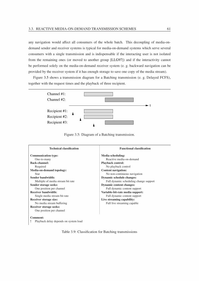
3.3. REACTIVE MEDIA-ON-DEMAND TRANSMISSION SCHEMES 61
any navigation would affect all consumers of the whole batch. This decoupling of media-on-
demand sender and receiver systems is typical for media-on-demand systems which serve several
consumers with a single transmission and is indispensable if the interacting user is not isolated
from the remaining ones (or moved to another group [LLG97]) and if the interactivity cannot
be performed solely on the media-on-demand receiver system (e. g. backward navigation can be
provided by the receiver system if it has enough storage to save one copy of the media stream).
Figure 3.5 shows a transmission diagram for a Batching transmission (e. g. Delayed FCFS),
together with the request times and the playback of three recipient.
Recipient #3:
t
Channel #2:
Channel #1:
Recipient #1:
Recipient #2:
Figure 3.5: Diagram of a Batching transmission.
Technical classification Functional classification
Communication type:
One-to-manyBack-channel:
RequiredMedia-on-demand topology:
StarSender bandwidth:
Multiple of media stream bit rateSender storage seeks:
One position per channelReceiver bandwidth:
Single media stream bit rateReceiver storage size:
No media stream bufferingReceiver storage seeks:
One position per channel
Media scheduling:
Reactive media-on-demandPlayback control:
No playback controlContent navigation:
No non-continuous navigationDynamic schedule changes:
Full dynamic scheduling change supportDynamic content changes:
Full dynamic content supportVariable-bit-rate media support:
Full dynamic content supportLive streaming capability:
Full live streaming capable
Comment:
! Playback delay depends on system load
Table 3.9: Classification for Batching transmissions
62 CHAPTER 3. MEDIA TRANSMISSION SCHEMES
3.3.3 Adaptive Piggy-Backing
While Batching benefits from one-to-many transmissions by allowing several recipients to listen to
one media stream, the Adaptive Piggy-Backing transmission scheme [GLM95, GLM96, AWY96a]
introduced a completely new approach to reduce the bandwidth in media-on-demand transmis-
sions: The basic idea of the Adaptive Piggy-Backing transmission scheme is that a recipient can
benefit from other ongoing transmissions of the same media stream.
The Adaptive Piggy-Backing transmission scheme accomplishes this by joining a new and an
ongoing transmission at some time. To bring two media stream transmissions to the same time
of transmission without interrupting the old one or skipping part of the transmission in the new
one, the display frame rate of the transmissions is modified at the receiver system for the Adaptive
Piggy-Backing transmission scheme. This allows delaying the ahead-running transmission and
to speed-up the later transmission until both transmissions reach the same point in the media
stream. A bandwidth gain is then achieved because the channel of one of the transmissions can be
terminated and used for the next request when the transmissions have been joined.
The authors of the article describing the Adaptive Piggy-Backing transmission scheme also
stated that
[. . . ] the video editing industry have assured [them] that alterations of the actual
display rate in the 2-3 % range or expansion and contraction (through interpolation)
in the 8 % range can be accomplished without being noticeable to the viewer.
But even if one media stream is expanded by 8 % and the next following one contracted by 8 %,
two requests can only be merged if the time between their arrivals is shorter than 16 % of the media
duration. For example for a two hour media stream, the requests can only be merged if the second
request arrives within 19.2 minutes after the first one. And the bandwidth reduction is very small,
even when the offset of the second request is as near as 9.6 minutes, only the half media stream
transmission can be left out.
Another drawback of this approach is that this creates additional requirements to the display
system: Assuming a transmission which includes a visual stream, the display system must be
able to adapt its frame rate to the display frame rate which has been determined by the Adaptive
Piggy-Backing transmission scheme. If this is not supported by the display system, interpolated
frames have to be inserted into or surplus frames have to be deleted from the transmitted stream
for presentation to adjust the display frame rate. These changes typically cause irritating judders
and thereby reduce the media quality significantly during presentation.
In [GLM95, GLM96], four different algorithms for the selection of the streams for which to
adjust the display frame rate have been proposed:
• Odd-Even Reduction Policy: The media stream for the first request is adjusted to the

3.3. REACTIVE MEDIA-ON-DEMAND TRANSMISSION SCHEMES 63
lowest possible bit rate, the next request (within a given window) uses the maximum bit
rate until the streams merge. If the next request arrives very late (e. g. at a time so it cannot
be merged) or if a third request arrives, the algorithm is restarted, serving the request again
using the lowest possible bit rate.
• Simple Merging: For the first stream, the lowest bit rate is used, for all further streams
within a fixed window the maximum bit rate is used.
• Greedy Policy: Same as odd-even policy, but after a merging or when reaching the window
when no other stream can merge to it, the algorithm is applied again to this stream. This
way, merged streams can be merged to other merged ones.
• Limited Merging: Merging is restricted to a predefined first part of the media, so the whole
media needs not to be available using several bit rates on the sender system.
For the Adaptive Piggy-Backing transmission scheme, a new type of diagram is needed as the
merging process is not clearly visible in the channel-based type of diagram which has been used
to illustrate the previously described transmission schemes. In stream-oriented diagrams, each
stream transmission is represented by a diagonal line. The bit rate of the transmission is shown by
the slope of the line, and a premature termination of a channel can be identified by the fact that
the line does not reach the height of the end stream marker at the left, vertical axis. Horizontal,
dashed lines are sometimes added at the premature termination of a stream to show which stream
is used to continue the playback. (This only applies to transmission schemes which buffer data.
For Adaptive Piggy-Backing, the continuation stream meets the terminating stream, so this line is
not necessary.)
Figure 3.6 shows a transmission diagram for the Adaptive Piggy-Backing transmission scheme,
illustrating the playback of three recipients. The transmission of the second recipient could be
merged to the first one in this example.
3.3.4 Patching
Patching [HCS98b] uses the same idea as Adaptive Piggy-Backing to reduce the bandwidth of the
sender system: Recipients benefit from other ongoing transmissions of the same media stream.
But instead of modifying the display frame rate of transmissions, Patching requires that the clients
receive data from another transmission concurrently to the reception and playback of the actual
transmission.
Therefore, two types of transmissions are possible for the Patching scheme: Firstly, the sender
system can transmit a media stream in its whole, as it has been done in the Batching scheme. The
first request for a media stream is always served using such a full transmission. But secondly,
if a request arrives a short time after a full transmission has been started, the sender system can

64 CHAPTER 3. MEDIA TRANSMISSION SCHEMES
Channel #3:
t
Channel #2:
Channel #1:
Recipient #1:
Recipient #2:
Recipient #3:
(a) Adaptive Piggy-Backing in a channel-based diagram
Recipients
Str
eam
Tra
nsm
issi
on
t#1 #2 #3
(b) Adaptive Piggy-Backing in a transmission-based diagram
Figure 3.6: Diagram of an Adaptive Piggy-Backing transmission.
decide to send only the “missed” part to the recipient. The recipient has to listen to both the new
patch transmission and the ongoing full transmission in this case, buffering the data of the full
transmission and “patching” the parts together when playing.
While full transmissions must be sent using one-to-many transmissions, the patch transmission
can use either one-to-one transmissions (if the recipient request is to be served immediate), or
one-to-many transmissions (if several recipients are served with the patch transmission, e. g. if
Batching is used to collect several requests).
As already mentioned above, the Patching scheme introduces two new requirements to the
receiver system compared to the Batching scheme:
• The receiver system must be able two receive two transmissions at the same time, so the
bandwidth requirement of the receiver system is twice the (maximum) media stream bit
rate.

3.3. REACTIVE MEDIA-ON-DEMAND TRANSMISSION SCHEMES 65
Technical classification Functional classification
Communication type:
One-to-manyBack-channel:
RequiredMedia-on-demand topology:
StarSender bandwidth:
Multiple of media stream bit rateSender storage seeks:
One position per channelReceiver bandwidth:
Single media stream bit rateReceiver storage size:
No media stream bufferingReceiver storage seeks:
One position per channel
Media scheduling:
Reactive media-on-demandPlayback control:
No playback controlContent navigation:
No non-continuous navigationDynamic schedule changes:
Full dynamic scheduling change supportDynamic content changes:
No dynamic content supportVariable-bit-rate media support:
No dynamic content supportLive streaming capability:
Full live streaming capable
Comment:
! Display frame rate depends on merging strategies
Table 3.10: Classification for Adaptive Piggy-Backing transmissions
• The receiver system must have a buffer where the data of the full transmission is stored
while the patch stream is played.
The efficiency of the Patching scheme depends very much on the decision when a full trans-
mission is to be started for an incoming request and when a patch stream is used instead. Unfor-
tunately, using patch transmissions whenever possible does not always result in the lowest band-
width consumption as illustrated in figure 3.7: In figure 3.7a, both transmissions #2 and #3 merge
to transmission #1, resulting in a total of 2.5 media stream transmissions, whereas in figure 3.7b
only transmission #3 merges to the previous full transmission #2 and the needed bandwidth totals
to 136 ≈ 2.17 media stream transmissions.
Recipientt
Str
eam
Tra
nsm
issi
on
#1 #2 #3
(a) Both streams #2 and #3 patch to the full transmission#1
Recipientt
Str
eam
Tra
nsm
issi
on
#1 #2 #3
(b) Only the last stream #3 patch to the preceding fulltransmission #2
Figure 3.7: Two different ways for the transmission of three media streams using patching.

66 CHAPTER 3. MEDIA TRANSMISSION SCHEMES
Another problem arises if the buffer size of the recipient system is not large enough to hold
half of the media stream. (It is not possible that the receiver system has to buffer more than half of
the media stream as only two transmissions are received and one of them is played immediately.)
In [HCS98b, CHV99], some algorithms for the merge decision have been proposed for this case:
• Greedy Patching: If the client buffer is too small for the missed part, the last part of the full
transmission is buffered and the patch has to transmit the remainder.
• Grace Patching: If the client buffer is too small for the missed part, a new full transmission
is scheduled.
• Patching with Fixed Window: If the client request arrives within a fixed window after a
full transmission, only the patch is transmitted, otherwise a new full transmission is started.
For this algorithm, the client buffer must be large enough to store a part of the media stream
of the size of the fixed window.
• Optimal Patching [CHV99, GT01, GT99]: Same as patching with fixed window, but the
window size is calculated using the request arrival rate of the recipients. Assuming a Poisson
distribution of the client requests, this algorithm calculates the window size so that the
average bandwidth is minimized.
Figure 3.8 shows the four different approaches how a receiver request is handled if it arrives so
late that the missed part cannot be cached by the client. To emphasize the differences, a very small
buffer has been chosen.
The authors of [BNL04] provided an algorithm of complexity O(n2) for calculating the optimal
merge decisions for a set of request times. Although this algorithm cannot be used in a practical
environment (as the request times are normally not known in advance), it is possible to use this
algorithm to examine the theoretical limit which can be reached by the Patching transmission
scheme at all.
3.3.5 Tapping
Tapping [CL97, SGRT99] can be seen as an improved version of Patching4. While the Patching
scheme only differentiated two types of transmissions — full transmissions and patch transmis-
sions — the Tapping transmission scheme uses three classes: original streams for full transmis-
sions, full tap streams for patch transmissions and partial tap streams as new class of transmis-
sion.
Partial tap streams are used when a stream should be merged to another transmission but the
buffer of the receiver system is too small to save the missed part of the transmission. For partial
4Strictly speaking, Tapping has been published before Patching, so Patching has to be looked at as a simplifiedversion of Tapping. But for better understanding, Patching has been presented before Tapping in this thesis.

3.3. REACTIVE MEDIA-ON-DEMAND TRANSMISSION SCHEMES 67
Buffer Size
Str
eam
Tra
nsm
issi
on
Full Patch Greedy Patcht
(a) Greedy Patching
Buffer Size
Str
eam
Tra
nsm
issi
on
Full Patch Fullt
(b) Grace Patching
t
Str
eam
Tra
nsm
issi
on
Full FullPatch
Window Size
(c) Patching with Fixed Window
t
Str
eam
Tra
nsm
issi
on
Full Patch Full Full PatchPatch
Window Size Changed Window Size
(d) Optimal Patching
Figure 3.8: Four different Patch transmission strategies.
Technical classification Functional classification
Communication type:
One-to-manyBack-channel:
RequiredMedia-on-demand topology:
StarSender bandwidth:
Multiple of media stream bit rateSender storage seeks:
One position per channelReceiver bandwidth:
! Twice the media stream bit rateReceiver storage size:
Partial media stream bufferingReceiver storage seeks:
One position per channel
Media scheduling:
Reactive media-on-demandPlayback control:
No playback controlContent navigation:
No non-continuous navigationDynamic schedule changes:
Full dynamic scheduling change supportDynamic content changes:
No dynamic content supportVariable-bit-rate media support:
No dynamic content supportLive streaming capability:
Full live streaming capable
Table 3.11: Classification for Patching transmissions
tap streams, the buffer of the receiver system is first filled with the data of the ongoing original
transmission until it is full. When the data of the tap stream reaches the buffered position, the
transmission on the tap stream can be interrupted and the receiver system can play the buffered
data. While playing data from the buffer and therefore emptying it, the receiver system again

68 CHAPTER 3. MEDIA TRANSMISSION SCHEMES
listens for new data from the original transmission and saves it into the buffer. When the data of
the buffer has been played, the stream is again continued at the tap stream, until the position in the
buffer is reached and the procedure is repeated. Figure 3.9 shows this in an example.
2 4 6
Buffer Size
7654321
7654321
7531
7654321
t
Channel #2:
Channel #1:
Recipient #1:
Recipient #2:
of Recipient #2:Buffer Content
Figure 3.9: Example of a full transmission and a partial tap stream transmission together with thebuffering
Figure 3.10 shows a (greedy) Patching transmission compared to an original Tapping trans-
mission, a Tapping transmission using extra tapping and a Tapping transmission using stream
stacking.
Buffer Size
Str
eam
Tra
nsm
issi
on
Full Patch Greedy Patcht
(a) Greedy Patching
Partial Tap
Buffer Size
Str
eam
Tra
nsm
issi
on
Fullt
(b) Tapping
Partial Tap
Buffer Size
Str
eam
Tra
nsm
issi
on
tFull
Full Tap
(c) Extra Tapping
Partial Tap #2
Buffer Size
Str
eam
Tra
nsm
issi
on
Fullt
FullPartial Tap #1
(d) Tapping with Stream Stacking
Figure 3.10: Comparison of Patching and Tapping.
The idea of Tapping has also been published from other authors under the terms Generalized

3.3. REACTIVE MEDIA-ON-DEMAND TRANSMISSION SCHEMES 69
Buffer Reuse Patching or Optimized Patching [SGRT99]. Additionally, in [Pâr01c], the authors
improved the performance of Tapping by preloading a part of the media stream to the receiver
system some time before the stream is requested. The effects of partial preloading are examined
in detail in section 4.6.
If the receiver system can receive more than two streams at once, extended versions of Tap-
ping [CL99, CLP00] can be used:
• Extra tapping: The receiver system can tap to any ongoing stream transmission, not only
to the original transmission.
• Stream stacking: When the receiver system has space left in its buffer and another channel
is not used at the moment (e. g. a partial tap stream), the order of the transmissions may be
rearranged, using the suspended other channel for the transmission. This does not reduce
the total bandwidth to transmit but allows releasing channels earlier.
Technical classification Functional classification
Communication type:
One-to-manyBack-channel:
RequiredMedia-on-demand topology:
StarSender bandwidth:
Multiple of media stream bit rateSender storage seeks:
One position per channelReceiver bandwidth:
! Twice the media stream bit rateReceiver storage size:
Partial media stream bufferingReceiver storage seeks:
One position per channel
Media scheduling:
Reactive media-on-demandPlayback control:
No playback controlContent navigation:
No non-continuous navigationDynamic schedule changes:
Full dynamic scheduling change supportDynamic content changes:
No dynamic content supportVariable-bit-rate media support:
No dynamic content supportLive streaming capability:
Full live streaming capable
Table 3.12: Classification for Tapping transmissions
3.3.6 Merging
Merging [EVZ99b, EVZ99a, EVZ01] is the most generalized version of Patching and Tapping:
The Merging scheme allows receiver systems to be merged to any stream, not only to full trans-
missions.
This improves the performance, but at the same time it increases the complexity at the sender
side: The sender system must not only decide if a full or patch transmission should be used for a
request, all merge decisions have to be evaluated.

70 CHAPTER 3. MEDIA TRANSMISSION SCHEMES
Merging is a very efficient transmission scheme for media-on-demand, and several strategies
which streams to merge with which other stream have been proposed:
• Earliest Reachable Merge Target (ERMT) [EVZ99b, EVZ99c]: For the Earliest Reach-
able Merge Target strategy, the first possible merge target is selected when the merging
process of all (yet) existing streams is simulated.
• Simple Reachable Merge Target (SRMT) [EVZ99b, EVZ99c]: As the decision for Earli-
est Reachable Merge Target is very complicated to calculate in large systems, this strategy
uses a more simple one: A merge target is only selected if the merge time of the merge target
with its immediately preceding stream lies behind the start time of the examined stream.
• Closest Target (CT) [EVZ99b, EVZ99c]: Another simplification of the Earliest Reachable
Merge Target strategy is to always merge to the closest preceding stream which still exists
and restart the search when the chosen stream terminates as it merged to another stream.
• Dyadic Stream Merging (2-Dyadic) [CJM02]: For the Dyadic Stream Merging strategy,
the interval of a full playback is divided into dyadic intervals of parameter 2 (i. e. into inter-
vals which are obtained by splitting the interval into two halves and recursively continuing
splitting the first half interval again and again). The first request of the second half always
starts a new full transmission in this scheme, therefore no requests of the second half have
to be considered here. For requests of the first half, the first request in each of the dyadic
intervals is merged directly to the full transmission. For the remaining request, the intervals,
starting at these requests until the end of their dyadic interval are again split into dyadic
intervals and requests in them are merged in the same manner, continuing until all requests
have been processed.
• Dyadic Stream Merging with golden ratio (φ-Dyadic) [BNGLT02]: This strategy uses
the same merging algorithm as the Dyadic Stream Merging strategy, but instead of halving
intervals, they are split according to the golden ratio 1+√
52 [BS91]. The authors of the Dyadic
Stream Merging strategy have proven that this is the optimal merging strategy for Poisson
distributed request arrivals if the requests are not known in advance.
• Optimal stream forest calculation [LLG98, BNL04]: For a given list of request times it is
possible to calculate the optimal merging combinations in O(n2) using dynamic program-
ming. This approach cannot be used in real environments as the list of request times is not
known in advance.
• Optimal off-line merging trees [BNGL03]: For a pro-active transmission scheme (some-
times called off-line transmission scheme), it is possible to compute merging trees in ad-
vance. The optimal merging trees in this case are Fibonacci trees, i. e. trees which are

3.3. REACTIVE MEDIA-ON-DEMAND TRANSMISSION SCHEMES 71
defined by a recursive, Fibonacci-like function:
S(i) =
⎧⎪⎨⎪⎩
the single node i if i ≤ 2
the tree obtained by adding S(i−2) as
last child to the root node of S(i−1)if i > 3
(3.17)
Figure 3.11 shows an example how one request pattern is handled differently by the ERMT,
SRMT, CT, 2-Dyadic, φ-Dyadic and optimal off-line merging strategies.
Str
eam
Tra
nsm
issi
on
E FCBA D Gt
(a) ERMT Stream Merging
Str
eam
Tra
nsm
issi
onE FCBA D G
t
(b) SRMT Stream Merging
Str
eam
Tra
nsm
issi
on
E FCBA D Gt
(c) CT Stream Merging
Str
eam
Tra
nsm
issi
on
E FCBA D Gt
(d) 2-Dyadic Stream Merging
Str
eam
Tra
nsm
issi
on
E FCBA D Gt
(e) φ-Dyadic Stream Merging
Str
eam
Tra
nsm
issi
on
t
(f) Optimal Off-line Stream Merging
Figure 3.11: Comparison of different Stream Merging strategies.
3.3.7 Virtual Batching
Virtual Batching (sometimes also referred to as Chaining) [SHH97, SHT97] differs from the above
transmission schemes by requiring that each receiver system can send a media stream to another
receiver system. Virtual Batching uses this capability to create chains of receivers, where each re-

72 CHAPTER 3. MEDIA TRANSMISSION SCHEMES
Technical classification Functional classification
Communication type:
One-to-manyBack-channel:
RequiredMedia-on-demand topology:
StarSender bandwidth:
Multiple of media stream bit rateSender storage seeks:
One position per channelReceiver bandwidth:
Multiple of media stream bit rateReceiver storage size:
Partial media stream bufferingReceiver storage seeks:
One position per channel
Media scheduling:
Reactive media-on-demandPlayback control:
No playback controlContent navigation:
No non-continuous navigationDynamic schedule changes:
Full dynamic scheduling change supportDynamic content changes:
No dynamic content supportVariable-bit-rate media support:
No dynamic content supportLive streaming capability:
Full live streaming capable
Table 3.13: Classification for Merging transmissions
ceiver passes the media stream data to another receiver with a delay (which is realized by buffering
the data before passing it). Whenever a new recipient requests the media stream before the buffer
of the last recipient in the chain was exhausted, the new recipient can simply be added to the end
of the chain, otherwise the receiver system becomes the first system in a new chain. Figure 3.12
illustrates this with five receiver systems in two chains, showing the used buffer size of the receiver
systems as bars below them.
Using receiver systems as further senders reduces the bandwidth requirements of the sender
system a lot, but induces several problems:
• At first, the receiver systems must be able to send the media stream to another receiver
system. This is probably the biggest problem as the upstream bandwidth of the receiver
system often does not provide enough bandwidth (if available anyhow).
• The receiver system must provide means for resource reservations: It has to provide buffer
space for delaying the media stream in the chain and it has to reserve bandwidth for sending
the media stream to the next system in the chain.
• The media transmission system is more error-prone as it requires proper working of receiver
systems. For example, switching a receiver system off or a power failure at one of the
receiver system breaks the chain and causes an abortion of the stream transmission at all
systems in the tail of the chain.
• All receiver systems in the chain must be trusted that they send the data unmodified. Prob-
ably, the media stream has to be signed using an asymmetrical algorithm, so the recipient
systems can check if the media stream has not been altered.

3.3. REACTIVE MEDIA-ON-DEMAND TRANSMISSION SCHEMES 73
Recipient #5:
t
Sent by sender system:
Sent by recipient #1:
Sent by sender system:
Sent by recipient #3:
Sent by recipient #4:
Recipient #1:
Recipient #2:
Recipient #3:
Recipient #4:
(a) Virtual Batching Transmissions
Recipient #1
Sender Media Database
Buffer of
Recipient #1
Recipient #2
Recipient #3
Recipient #4
Recipient #5
(b) Chains in Virtual Batching Transmission
Figure 3.12: Example of a Virtual Batching transmission
• It may be undesirable that a receiver system can detect its successor system in the chain for
privacy reasons.
3.3.8 Peer-to-Peer Networks
A generalization of Virtual Batching is provided by Peer-to-Peer Networks: In a Peer-to-Peer
Network, the sender and receiver roles are merged to a single peer role, so every node can consume
data and provide data at the same time.
Similar to some advanced media-on-demand transmission schemes, today’s Peer-to-Peer Net-
works split files into several small parts which are retrieved separately and finally concatenated. In

74 CHAPTER 3. MEDIA TRANSMISSION SCHEMES
Technical classification Functional classification
Communication type:
One-to-manyBack-channel:
Required, supporting media bit rate to anotherrecipient
Media-on-demand topology:
StarSender bandwidth:
Multiple of media stream bit rateSender storage seeks:
One position per channelReceiver bandwidth:
! Single media stream bit rateReceiver storage size:
Partial media stream bufferingReceiver storage seeks:
One position per channel
Media scheduling:
Reactive media-on-demandPlayback control:
No playback controlContent navigation:
No non-continuous navigationDynamic schedule changes:
Full dynamic scheduling change supportDynamic content changes:
No dynamic content supportVariable-bit-rate media support:
No dynamic content supportLive streaming capability:
Full live streaming capable
Comment:
! Receiver systems must forward media streams
Table 3.14: Classification for Virtual Batching transmissions
contrast to advanced media-on-demand transmission schemes where the splitting of media streams
into segments is used to lower the total bandwidth consumption for a media stream transmission to
several recipients, the reason for splitting them in Peer-to-Peer Networks only serves the purpose
to lower the send bandwidth requirements of the peers5. The total bandwidth consumption for me-
dia stream transmissions using Peer-to-Peer Networks will still be the same as for Point-to-Point
Transmissions because no multicasting transmissions are used.
Similar to Virtual Batching, Peer-to-Peer Networks have several drawbacks if used for media-
on-demand (i. e. if the media stream is transmitted on request and consumed concurrently to its
reception):
• The peer must be able to send the media stream to another peer. In contrast to Virtual
Batching, the peer must not support sending the media stream at full media bit rate if several
peers send the media stream together to a receiving peer.
• The peer must provide means for resource reservations: As for Virtual Batching, buffer
space and bandwidth for sending media stream segments must be reserved.
• The Peer-to-Peer Network will fail to work if the total media bandwidth of all active requests
exceeds the total transmission bandwidth of all peers. As peers in Peer-to-Peer Networks
have often only a low upstream bandwidth (e. g. using ADSL), the upstream bandwidth of
5The peers of Peer-to-Peer Networks have often only a low upstream bandwidth (e. g. using ADSL), so severalpeers are combined in a Peer-to-Peer Network to transmit the file in an acceptable time.

3.3. REACTIVE MEDIA-ON-DEMAND TRANSMISSION SCHEMES 75
several peers is required for the transmission of one media stream to a requesting peer. This
disallows using Peer-to-Peer Networks for media-on-demand when it is possible that a high
ratio of the peers is requesting a media stream concurrently.
• The peer must provide real-time semantics so each segment is available in due time when
needed for playback. Peer-to-peer software which is currently used for file distribution does
not provide any timing constraints for transmissions. This makes it currently unusable for
real-time transmissions like media-on-demand stream transmissions.
• The last three bullets of the list of drawbacks of Virtual Batching (more error-prone, security
considerations, privacy concerns) apply to Peer-to-Peer Networks, too.
Technical classification Functional classification
Communication type:
One-to-manyBack-channel:
RequiredMedia-on-demand topology:
MeshSender bandwidth:
AnySender storage seeks:
One position per channelReceiver bandwidth:
Single media stream bit rateReceiver storage size:
Full media stream bufferingReceiver storage seeks:
One position per channel
Media scheduling:
Reactive media-on-demandPlayback control:
No playback controlContent navigation:
No non-continuous navigationDynamic schedule changes:
No dynamic scheduling change supportDynamic content changes:
No dynamic content supportVariable-bit-rate media support:
No dynamic content supportLive streaming capability:
Not live streaming capable
Comment:
! Receiver systems must forward partial media streams
Table 3.15: Classification for Peer-to-Peer transmissions
3.3.9 Comparison of Reactive Transmission Schemes
A comparison of the above reactive transmission schemes is very difficult as the schemes differ in
many parameters, e. g.:
• average needed bandwidth of the sender system,
• maximum of needed bandwidth of the sender system,
• disposable bandwidth of the sender system,
• maximum bandwidth capacity of the receiver system,

76 CHAPTER 3. MEDIA TRANSMISSION SCHEMES
• maximum storage requirements of the receiver system,
• playback request pattern,
• average playback delay,
• maximum playback delay,
To get an overview of the efficiency, the following assumptions are made for the forthcoming
comparison:
• Playback requests are Poisson distributed with parameter λ.
• Receiver systems have enough storage to buffer any necessary amount of media data.
• The transmission of a single media stream is examined.
The first of these assumptions can be accepted as long as requests from different receiver sys-
tems are independent from each other (see section 3.1.1). The second assumption can be validated
by observing the steadily falling costs of memory and hard disk storage: Memory is nowadays
cheaper than EUR 20 per gigabyte, and hard disks are available for EUR 0.20 per gigabyte, mak-
ing tight restrictions on storage requirements nearly obsolete. The restriction to a single media
stream is valid as long as all media transmissions are independent from each other.
Using these assumptions, the following schemes can be omitted in the comparison:
• FCFS Batching, MQL Batching and MFQL Batching only differ in the way how they handle
requests for different media streams. Because of restriction three, these Batching schemes
give equal results in this comparison.
• Prioritized Queuing Batching assumes different classes of recipients. This favors some re-
quests by penalizing other ones, but the overall performance is lowered.
• The Adaptive Piggy-Backing transmission scheme modifies the display rate of the media
stream to accomplish merges. As this violates the real-time constraint of media-on-demand
transmission schemes (see section 1.1), the Adaptive Piggy-Backing scheme is excluded
here.
• The different Patching schemes assume limited receiver storage. Due to restriction two, only
Patching with sufficient large storage space and an optimal patching window (calculated
according to [EVZ99a, EVZ01] from the average request rate) is used.
• The Tapping schemes are equivalent to Patching if no limit on the storage size of the recipi-
ent systems is imposed.
• Virtual Batching and Peer-to-Peer Networks are omitted as they use recipient systems as
additional senders.

3.3. REACTIVE MEDIA-ON-DEMAND TRANSMISSION SCHEMES 77
To compare the remaining transmission schemes, they are evaluated using simulated, Poisson
distributed client requests of different request rates. Each simulation is run 50 times and the
observed interval is chosen each time to contain 5 000 requests to get meaningful results.
For transmission schemes which provide immediate service, the efficiency of the transmission
scheme is then retrieved by calculating the minimum required bandwidth using the formula given
in section 3.1.2 and dividing this value by the average bandwidth of the simulations as described
in section 3.1. Figure 3.13 shows the results for request rates between 1 and 1 000 requests per
media stream duration.
The results of the Optimal Merge Decision Patching algorithm (see section 3.3.4) have been
included in this graph although it requires knowledge of the request times in advance. As this
knowledge gives the algorithm an advantage to transmission schemes which have to react on ran-
dom request patterns, it has a higher efficiency. For low request rates, its “efficiency” is even higher
than 100 % as the efficiency calculation assumes a random Poisson process for the distribution of
requests without knowledge of future requests.
For the Point-to-Point transmission scheme, a receiver bandwidth equal to the media bit rate has
to be asserted. Under this precondition, the Point-to-Point transmission scheme has an efficiency of
100 % as it is the optimal (and apart from channel permutations the only) solution which provides
immediate service if the receiver systems cannot receive more than the media bit rate. To prove
that the Point-to-Point transmission scheme looses its attractiveness if the receiver bandwidth is
not limited to the media stream bit rate, the efficiency of the Point-to-Point transmission scheme
has been added a second time to the graph for the case that the receiver system is able to receive
twice the media bit rate.
Besides of this special case for the Point-to-Point transmission scheme, it is clearly visible
that the ERMT Merging algorithm has the highest efficiency of all reactive transmission schemes.
Another important point about reactive transmission schemes is that they are less efficient for high
media request rates.
For the Batching transmission scheme which serves requests delayed, the bandwidth require-
ments are measured for a maximum playback delay of 1120 of the media stream duration (which
corresponds to a playback delay of one minute for a two hour media stream) and compared to the
theoretical minimum to calculate the efficiency of this scheme. Figure 3.14 shows the result of
this analysis. As for the Point-to-Point transmission scheme, the Batching transmission scheme
requires only a receiver bandwidth equal to the media bit rate and has an efficiency of nearly
100 % under this precondition. As above, the efficiency of the Batching scheme for a receiver
bandwidth of twice the media bit rate has been added to the graph to make it comparable with
other transmission schemes if this precondition is not necessary.

78 CHAPTER 3. MEDIA TRANSMISSION SCHEMES
10%
20%
30%
40%
50%
60%
70%
80%
90%
100%
1 2 5 10 20 50 100 200 500 1000
Ban
dwid
th e
ffic
ienc
y
Average number of requests per media stream duration
Point-to-Point (R=1)Optimal Merge Decision Patching
ERMT MergingCT Merging
Phi-Dyadic Merging2-Dyadic MergingOptimal Patching
SRMT MergingPoint-to-Point (R=2)
Figure 3.13: Comparison of efficiency of reactive transmission schemes with immediate service
10%
20%
30%
40%
50%
60%
70%
80%
90%
100%
1 2 5 10 20 50 100 200 500 1000
Ban
dwid
th e
ffic
ienc
y
Average number of requests per media stream duration
Batching (R=1)Batching (R=2)
Figure 3.14: Efficiency of reactive transmission schemes with delayed service
3.4 Non-Segmenting Pro-Active Transmission Schemes
In the last section, reactive transmission schemes have been examined. Starting with this section
and extending up to section 3.7, the large group of pro-active transmission schemes is examined.

3.4. NON-SEGMENTING PRO-ACTIVE TRANSMISSION SCHEMES 79
In contrast to reactive schemes which transfer media streams (immediately or with some delay)
as a result of individual request from consumers, pro-active transmission schemes transmit media
streams continuously, independent of any requests. This has several advantages over reactive
schemes:
• Playback requests must not be forwarded from the receiver system to the sender system, it
is actually possible to drop any communication from the receiver system towards the sender
system.
• Resource requirements (bandwidth, memory) and service guarantees (playback delay) can
be calculated independent of the number of concurrent transmissions and the pattern of
client requests.
• The needed server bandwidth for highly requested media streams is lower if a pro-active
scheme is used.
• The transmission schedule has not to be created dynamically but can be computed in ad-
vance which lowers the real-time requirements of the sender system and removes some
complexity.
The main disadvantage of a pro-active transmission scheme is that it cannot save bandwidth when
only few or even no recipients listen to the transmission. Solutions to this problem are addressed
in more detail in sections 3.8 and 4.20.1.
The remainder of this section describes two very old and simple pro-active transmission
schemes. These transmission schemes always transmit media streams as a whole and are gen-
erally only interesting because of their simplicity. Several more advanced schemes are presented
in the sections after this one in three groups, sorted by their functioning.
3.4.1 Round-Robin Broadcasting
A simple type of media-on-demand is to transmit one (or several) media streams per transmission
channel permanently in a round-robin manner. This type of media-on-demand is very popular in
small, ancient media-on-demand systems and can sometimes still be found in hotels. Its main
advantages are low system requirements: Besides of accounting, the media-on-demand receiver
system has no other requirements than a normal TV system, and at the sender side, usual video
cassette recorders with automatic rewind or endless tapes can be used. The main disadvantage
of Round-Robin Broadcasting is the high playback delay: In worst case, a consumer has to wait
nearly one whole media playback duration until the media stream is started again.
Figure 3.15 shows a transmission diagram for a Round-Robin Broadcasting transmission, to-
gether with the media playback by one recipient.

80 CHAPTER 3. MEDIA TRANSMISSION SCHEMES
Media Playback
t
Recipient:
Channel:
Media Request
Figure 3.15: Diagram of a Round-Robin Broadcasting transmission.
Technical classification Functional classification
Communication type:
One-to-manyBack-channel:
Not requiredMedia-on-demand topology:
StarSender bandwidth:
Single media stream bit rateSender storage seeks:
One position per channelReceiver bandwidth:
Single media stream bit rateReceiver storage size:
No media stream bufferingReceiver storage seeks:
One position per channel
Media scheduling:
Pro-active media-on-demandPlayback control:
No playback controlContent navigation:
No non-continuous navigationDynamic schedule changes:
Full dynamic scheduling change supportDynamic content changes:
Full dynamic content supportVariable-bit-rate media support:
Full dynamic content supportLive streaming capability:
Full live streaming capable
Comment:
! Maximum playback delay equals media stream duration
Table 3.16: Classification for Round-Robin Broadcasting transmissions
3.4.2 Staggered Broadcasting
An improvement to the Round-Robin Broadcasting scheme presented above is the Staggered
Broadcasting scheme (also known as Baseline transmissions) [PLE03]: For Staggered Broadcast-
ing transmissions, each media stream is transmitted several times in parallel, using different phase
shifts for each transmission. As a result, the playback delay is reduces to a fraction equivalent to
the reciprocal of the number of used channels.
Another improvement of this transmission scheme is the possibility to navigate within the
media stream: By changing to another transmission of the same media stream, the receiver system
can jump within the media stream in a limited way (fixed jump playback control).
Although the improvement over Round-Robin Broadcasting is very high, this transmission
scheme requires a lot of sender bandwidth, so the number of transmitted media streams is typically
low.

3.4. NON-SEGMENTING PRO-ACTIVE TRANSMISSION SCHEMES 81
Figure 3.16 shows a transmission diagram for a transmission using three channels for the Stag-
gered Broadcasting scheme, together with the playback by one recipient.
Channel #3:
t
Recipient:
Channel #2:
Channel #1:
Figure 3.16: Diagram of a staggered transmission.
Technical classification Functional classification
Communication type:
One-to-manyBack-channel:
Not requiredMedia-on-demand topology:
StarSender bandwidth:
Multiple of media stream bit rateSender storage seeks:
One position per channelReceiver bandwidth:
! Single media stream bit rateReceiver storage size:
No media stream bufferingReceiver storage seeks:
One position per channel
Media scheduling:
Pro-active media-on-demandPlayback control:
Fixed jump playback controlContent navigation:
No non-continuous navigationDynamic schedule changes:
Full dynamic scheduling change supportDynamic content changes:
No dynamic content supportVariable-bit-rate media support:
No dynamic content supportLive streaming capability:
Full live streaming capable
Comment:
! High server bandwidth requirements if short playback delays should be provided
Table 3.17: Classification for Staggered Broadcasting transmissions
3.4.3 Comparison of Non-Segmenting Pro-Active Transmission Schemes
Round-Robin Broadcasting transmissions and the Staggered Broadcasting transmission scheme
are two very simple but widely used versions for pro-active media-on-demand. Their main advan-
tages lay in the low requirements for the receiver systems and their simplicity for both sender and
receiver systems. But for short playback delays, they are practically of no use:
• For the Round-Robin Broadcasting scheme, no modification of the playback delay is possi-
ble, the worst case playback delay is always equal to the media stream duration.
82 CHAPTER 3. MEDIA TRANSMISSION SCHEMES
• For the Staggered Broadcasting scheme, the required bandwidth is inversely proportional
to the playback delay, i. e. the bandwidth at the sender system increases very fast if the
playback delay becomes small.
The efficiency of the Round-Robin Broadcasting scheme is 100 % for the single set of sup-
ported parameters (playback delay equals stream duration), but as no modification of the playback
delay is supported, the use of this transmission scheme is very limited.
Calculating the efficiency for the Staggered Broadcasting scheme depends very much on the
prerequisites: Assuming that the receiver system can only receive one channel at media stream bit
rate, it is not possible to create a pro-active transmission scheme with lower bandwidth require-
ments than the Staggered Broadcasting scheme provides, i. e. the efficiency η is 100 %.
But if the receiver systems can receive more than a single channel at media stream bit rate, the
efficiency decreases very fast for short playback delays. For example, if a playback delay of 1120 of
the media stream duration is desired (which equals a playback delay of one minute for a two hour
media stream) and the receiver system is able to receive six times the media bit rate (which is
the bandwidth needed by one of the advanced transmission scheme presented later for the same
setup), the efficiency of the Staggered Broadcasting scheme is only6
η =
Ψ0
(1+ 1
1201
7200
)−Ψ0
( 1120
17200
)120
=Ψ0(7260)−Ψ0(60)
120≈ 4.0% (3.18)
3.5 Size-Based Segmenting Transmission Schemes
The last section introduced the idea of pro-active transmission schemes with two very inefficient
approaches. Starting with this section and continued up to section 3.7, a group of advanced, much
more efficient, pro-active media-on-demand transmission schemes is examined.
One common fact for this group of schemes is that the media stream is not transmitted se-
quentially any more. Instead, the media stream is split into several segments, which are broadcast
according to a fixed or calculated transmission schedule by the sender system. On the receiver
system side, all received segments have to be saved for these schemes and must be reassembled
when they are needed for playback.
The main advantage of this segmentation procedure is that bandwidth can be saved: As receiver
systems do not need the later segments of a media stream until all preceding segments have been
played, these segments can be transmitted less frequently.
Three different ways how segmented transmissions can be performed have evolved:
6This calculation is based on equation (3.10) using a slot interval of δ = d7200 which equals segments of one second
in case of a two hour media stream.

3.5. SIZE-BASED SEGMENTING TRANSMISSION SCHEMES 83
• Size-based approach: All segments are transmitted in parallel at the same time using the
same bandwidth, but the segment sizes are increasing. This way, the size of a segment
determines the frequency for the transmission of the data of the segment, and increasing
the size for later segments of a stream therefore reduces the transmission frequency of these
segments.
• Bandwidth-based approach: The media stream is split into segments of equal size, which
are transmitted in parallel, using decreasing bandwidths. Using this approach, the band-
width determines the frequency for the segment transmissions. As the bandwidth for later
segments of a media stream is decreased, their transmission frequency is lowered.
• Frequency-based approach: The media stream is split into segments of equal size, which
are transmitted using the same bandwidth for all segments but only at increasing periodic
intervals. As the segment period determines the frequency for the segment transmission
in this approach, the frequency for the transmission of later segments of a media stream is
decreased by increasing the periods of these segments.
Figure 3.17 illustrates the the differences between these three approaches.
3 3
t
1 1 1 1 1
2 2
1 1 1 1 1 1
2 2 2 2 2 2 2
111111 1
3 3 3
(a) Size-based approach
1 1
2
10
1
.
1
..
1 1 1 1 1 1 1 1 1 1
t
1 1 1 1
(b) Bandwidth-based approach
4
1 1 1 1 1 1
2 4 2 5 2 4 2 5
3 6 8 3 7 9
t
3 6 8 3 7 9
2 4 2 5 2 4 2 5
3 6 8 3 7 9
1 1 1 1 1 11 1 1 1 1 1
2
(c) Frequency-based approach
Figure 3.17: Three different approaches for segmented media-on-demand transmissions
The remainder of this section describes transmission schemes which use the size-based ap-
proach, while transmission schemes of bandwidth-based and frequency-based approaches are de-
scribed in the next two sections 3.6 and 3.7, resp.

84 CHAPTER 3. MEDIA TRANSMISSION SCHEMES
3.5.1 Pyramid Broadcasting
The Pyramid Broadcasting scheme [VI96] was the first published transmission scheme which used
the segmenting approach. Although its origins lay rather in TV network based transmissions, it
can be used on any other multicast or broadcast capable network.
For the Pyramid Broadcasting scheme, each media stream is split into segments of geometri-
cally increasing size, i. e. the size of the i-th segment is αi−1 times the size of the first segment.
The parameter α thereby is chosen by the Pyramid Broadcasting Scheme in such a way that the
maximum playback delay is minimized. As the maximum playback delay W + can be calculated
from α and the number of channels N (which is the same as the number of segments n for the
Pyramid Broadcasting scheme) by
W+= d · α−1
α · (αN −1)(3.19)
it is only possible to calculate the optimum values for α by applying a numerical minimum search.
Table 3.18 shows the results of this calculation for two to eight channels.
Number of channels α
2 1.71053 2.05564 2.23975 2.34856 2.41837 2.46648 2.5012∞ e ≈ 2.7182
Table 3.18: Optimal values for the parameter α of the Pyramid Broadcasting scheme
For the Pyramid Broadcasting scheme, all media streams are transmitted on the same set of
channels, thus the total available bandwidth of the sender system is divided into as many channels
as segments are used in each media stream (which assumes that all media streams have the same
duration).
To receive a media stream, the receiver system has to join the first channel and has to wait for
the next transmission of the first segment of the desired media stream. The segment data is then
received into a buffer and the playback is started. While playing the segment, the receiver system
joins the next channel, waits for the beginning of the next segment and appends it to the buffer.
This procedure is continued until all segments have been received and played.
Figure 3.18 shows a media transmission using the Pyramid Broadcasting scheme for three
channels and two media streams (one consisting of segments 1 to 3, the other of segments A to C).
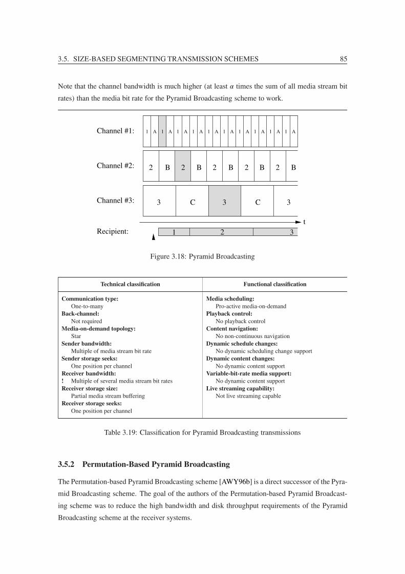
3.5. SIZE-BASED SEGMENTING TRANSMISSION SCHEMES 85
Note that the channel bandwidth is much higher (at least α times the sum of all media stream bit
rates) than the media bit rate for the Pyramid Broadcasting scheme to work.
Channel #1:
Channel #3:
tRecipient:
1
2 B 2 BB 2 B 2 B 2
3 C 3 C 3
A 1 A 1 A 1 A 1 A 1 A 1 A 1 A 1 A 1 A
1 2 3
Channel #2:
Figure 3.18: Pyramid Broadcasting
Technical classification Functional classification
Communication type:
One-to-manyBack-channel:
Not requiredMedia-on-demand topology:
StarSender bandwidth:
Multiple of media stream bit rateSender storage seeks:
One position per channelReceiver bandwidth:
! Multiple of several media stream bit ratesReceiver storage size:
Partial media stream bufferingReceiver storage seeks:
One position per channel
Media scheduling:
Pro-active media-on-demandPlayback control:
No playback controlContent navigation:
No non-continuous navigationDynamic schedule changes:
No dynamic scheduling change supportDynamic content changes:
No dynamic content supportVariable-bit-rate media support:
No dynamic content supportLive streaming capability:
Not live streaming capable
Table 3.19: Classification for Pyramid Broadcasting transmissions
3.5.2 Permutation-Based Pyramid Broadcasting
The Permutation-based Pyramid Broadcasting scheme [AWY96b] is a direct successor of the Pyra-
mid Broadcasting scheme. The goal of the authors of the Permutation-based Pyramid Broadcast-
ing scheme was to reduce the high bandwidth and disk throughput requirements of the Pyramid
Broadcasting scheme at the receiver systems.
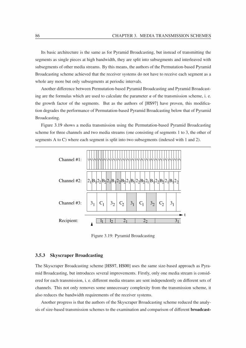
86 CHAPTER 3. MEDIA TRANSMISSION SCHEMES
Its basic architecture is the same as for Pyramid Broadcasting, but instead of transmitting the
segments as single pieces at high bandwidth, they are split into subsegments and interleaved with
subsegments of other media streams. By this means, the authors of the Permutation-based Pyramid
Broadcasting scheme achieved that the receiver systems do not have to receive each segment as a
whole any more but only subsegments at periodic intervals.
Another difference between Permutation-based Pyramid Broadcasting and Pyramid Broadcast-
ing are the formulas which are used to calculate the parameter α of the transmission scheme, i. e.
the growth factor of the segments. But as the authors of [HS97] have proven, this modifica-
tion degrades the performance of Permutation-based Pyramid Broadcasting below that of Pyramid
Broadcasting.
Figure 3.19 shows a media transmission using the Permutation-based Pyramid Broadcasting
scheme for three channels and two media streams (one consisting of segments 1 to 3, the other of
segments A to C) where each segment is split into two subsegments (indexed with 1 and 2).
A A1 1 1 1 1 1 1 1 1 1 1 1 1 1 1AAA2 2 2 2 2 2 2 2 2A1AA211111 22222222221 1 1 1
1 1 1 1 12 222
11 12 2212 13
Channel #1:
Channel #2:
Channel #3:
2
tRecipient:
3 3 3 3 3CC C C
1 1 1 1 1 1 1 1 1 1
1 1 11 1 12 2 2 2 2 1 2 12 2 12 22B B B B B B B B B122222 2 2
1 1 11 1A A A A A A A A A A A A
Figure 3.19: Pyramid Broadcasting
3.5.3 Skyscraper Broadcasting
The Skyscraper Broadcasting scheme [HS97, HS00] uses the same size-based approach as Pyra-
mid Broadcasting, but introduces several improvements. Firstly, only one media stream is consid-
ered for each transmission, i. e. different media streams are sent independently on different sets of
channels. This not only removes some unnecessary complexity from the transmission scheme, it
also reduces the bandwidth requirements of the receiver systems.
Another progress is that the authors of the Skyscraper Broadcasting scheme reduced the analy-
sis of size-based transmission schemes to the examination and comparison of different broadcast-

3.5. SIZE-BASED SEGMENTING TRANSMISSION SCHEMES 87
Technical classification Functional classification
Communication type:
One-to-manyBack-channel:
Not requiredMedia-on-demand topology:
StarSender bandwidth:
Multiple of media stream bit rateSender storage seeks:
One position per channelReceiver bandwidth:
! Multiple of several media stream bit ratesReceiver storage size:
Partial media stream bufferingReceiver storage seeks:
One position per channel
Media scheduling:
Pro-active media-on-demandPlayback control:
No playback controlContent navigation:
No non-continuous navigationDynamic schedule changes:
No dynamic scheduling change supportDynamic content changes:
No dynamic content supportVariable-bit-rate media support:
No dynamic content supportLive streaming capability:
Not live streaming capable
Table 3.20: Classification for Permutation-based Pyramid Broadcasting transmissions
ing series, where each broadcasting series simply describes the (relative) sizes of the segments of
the examined transmission scheme. For example, the broadcasting series of Pyramid Broadcasting
is the geometric series 1,α,α2,α3, . . . because the size of the i-th segment is αi−1 times the size of
the first segment for this transmission scheme.
For Skyscraper Broadcasting, a new broadcasting series has been introduced which is recur-
sively defined by the following function:
S(i) =
⎧⎪⎪⎪⎪⎪⎪⎪⎪⎪⎪⎪⎪⎪⎨⎪⎪⎪⎪⎪⎪⎪⎪⎪⎪⎪⎪⎪⎩
1 if i = 1,
2 if i = 2 or i = 3,
2 ·S(i−1)+1 if i ≥ 4, i mod 4 = 0,
S(i−1) if i ≥ 4, i mod 4 = 1,
2 ·S(i−1)+2 if i ≥ 4, i mod 4 = 2,
S(i−1) if i ≥ 4, i mod 4 = 3
(3.20)
The broadcasting series generated by this function starts with
1,2,2,5,5,12,12,25,25,52,52,105,105,212,212,425, . . . (3.21)
and results in shorter playback delays than the geometric series of Pyramid Broadcasting.
Another advantage of Skyscraper Broadcasting is that the broadcasting series can be adjusted to
the receiver systems storage size: If an upper bound is applied to the elements of the broadcasting
series, the required storage of the receiver system can be limited (at the cost of a longer playback

88 CHAPTER 3. MEDIA TRANSMISSION SCHEMES
delay or higher sender bandwidth requirements). In section 4.19, this approach is revived in the
context of a frequency-based transmission scheme.
Skyscraper Broadcasting uses channels which have the same bandwidth as the media stream
to transmit7 instead of high bandwidth channels which are required for Pyramid Broadcasting
and Permutation-based Pyramid Broadcasting. Of these channels, the receiver systems must be
able to receive two channels simultaneously for Skyscraper Broadcasting transmissions, but as
the channel bandwidth is much lower than for the Pyramid Broadcasting scheme, the bandwidth
requirements have been much relaxed for the receiver systems.
Figure 3.20 shows a media transmission using the Skyscraper Broadcasting scheme for five
channels.
4Recipient:
t
Channel #1:
Channel #2:
Channel #3:
Channel #4:
Channel #5: 5
4 4 4 4
5 5 5
1
2
3
1 1 1
2
3
1
2
3
1 1 1
2
3
1
2
3
1 1 1
2
3
1
2
3
1 1 1
2
3
1
2
3
1 1 1
2
3
1 2 3 5
Figure 3.20: Skyscraper Broadcasting
Technical classification Functional classification
Communication type:
One-to-manyBack-channel:
Not requiredMedia-on-demand topology:
StarSender bandwidth:
Multiple of media stream bit rateSender storage seeks:
One position per channelReceiver bandwidth:
! Twice the media stream bit rateReceiver storage size:
! Configurable media stream bufferingReceiver storage seeks:
One position per channel
Media scheduling:
Pro-active media-on-demandPlayback control:
No playback controlContent navigation:
No non-continuous navigationDynamic schedule changes:
No dynamic scheduling change supportDynamic content changes:
No dynamic content supportVariable-bit-rate media support:
No dynamic content supportLive streaming capability:
! Full live streaming capable
Table 3.21: Classification for Skyscraper Broadcasting transmissions
7Skyscraper Broadcasting does not support media streams which use a variable-bit-rate encoding.

3.5. SIZE-BASED SEGMENTING TRANSMISSION SCHEMES 89
3.5.4 Mayan Temple Broadcasting
The Mayan Temple Broadcasting scheme [PLM99] generalizes the Skyscraper Broadcasting
scheme in mainly three points: Firstly, it requires that the receiver system receives the data from
all channels at once. Although this increases the requirements for the receiver systems, the needed
sender bandwidth is reduced this way.
Secondly, it does not use a fixed broadcasting series but a function which calculates the size
of the segments from the cumulative bandwidth function of the media stream8. The major advan-
tage of this approach is that the Mayan-Temple Broadcasting scheme can support variable-bit-rate
media streams. As a consequence, the channel bandwidth can be selected independently from the
media stream bit rate, even for constant-bit-rate media streams.
Lastly, the Mayan Temple Broadcasting scheme supports a mechanism called partial preload-
ing. Partial preloading means that a part (sensibly the beginning) of the media stream is transmit-
ted to the recipient system before the client requests the media stream. By partial preloading, the
Mayan Temple Broadcasting scheme provides support for immediate playback. The disadvantage
of partial preloading is, that the beginnings of all media streams have to be transmitted periodi-
cally on an additional channel and have to be saved by the recipient systems for later playback.
The advantages and drawbacks of partial preloading will be reviewed in section 4.6.
The formula for the duration δi of segment i ≥ 2 of the Mayan Temple Broadcasting scheme is
given as:
δi = f−1
(f
(W
++
i−1∑j=2
δj
)+β ·
(W
++
i−1∑j=2
δj
))−W
++
i−1∑j=2
δj (3.22)
where f is the cumulative bandwidth function (see section 4.1.2), f−1 is the inverse cumulative
bandwidth function (see section 4.7.3) and β is the channel bandwidth. This formula can be
reduced to
δi =W+ ·
i−1∑j=1
(β
β1
)j
·(i−2
j−1
)(3.23)
if all segments have the same average bit rate β1 (which is esp. true for constant-bit-rate media
streams)9.
For a constant-bit-rate media stream and channels at media stream bit rate, this formula gener-
ates the following broadcasting series:
(1),1,2,4,8,16,32,64,128,256,512,1024,2048,4096,8192,16384, . . . (3.24)
8The cumulative bandwidth function describes the characteristics of the bit rate variations of a variable-bit-ratemedia stream. A definition of the cumulative bandwidth function is presented in section 4.1.2.
9Please take care when reading the article about the Mayan Temple Broadcasting scheme [PLM99] as in theirformula the binomial coefficient is accidentally missing.

90 CHAPTER 3. MEDIA TRANSMISSION SCHEMES
The first segment from this series is typically transmitted in advance (i. e. preloaded) for this trans-
mission scheme (denoted by the parenthesis in the broadcasting series) but may also be transmitted
on a separate channel if preloading is not used.
Figure 3.21 shows a media transmission using the Mayan Temple Broadcasting scheme for
four channels and a preloading of segment #1.
2
t
Channel #2:
Channel #3:
Channel #4:
2 2 2 2 2 2 2 2 2 2 2 2 2 2 2 2 2 2 2
3 3 3 3 3 3 3 3 3 3
4 4 4 4 4
5 5 5
Recipient: 1 2 3 4 5
Preloading:
Channel #1:
1
Figure 3.21: Mayan Temple Broadcasting
Technical classification Functional classification
Communication type:
One-to-manyBack-channel:
Not requiredMedia-on-demand topology:
StarSender bandwidth:
Multiple of media stream bit rateSender storage seeks:
One position per channelReceiver bandwidth:
Multiple of media stream bit rateReceiver storage size:
! Configurable partial preloadingReceiver storage seeks:
One position per channel
Media scheduling:
Pro-active media-on-demandPlayback control:
No playback controlContent navigation:
No non-continuous navigationDynamic schedule changes:
No dynamic scheduling change supportDynamic content changes:
No dynamic content supportVariable-bit-rate media support:
No dynamic content supportLive streaming capability:
! Full live streaming capable
Table 3.22: Classification for Mayan Temple Broadcasting transmissions
3.5.5 Client-Centric Approach
The Client-Centric Approach transmission scheme [HCS98a] has its origins at the Skyscraper
Broadcasting scheme, but it allows specifying the number of channels R which a receiver system
can join simultaneously. It uses another broadcasting series, which is defined by the following

3.5. SIZE-BASED SEGMENTING TRANSMISSION SCHEMES 91
function10:
SR(i) =
⎧⎪⎪⎪⎨⎪⎪⎪⎩
1 if i = 1,
2 ·S(i−1) if i ≥ 2, i mod R �= 1,
S(i−1) if i ≥ 2, i mod R = 1
= 2i−� iR
(3.25)
For R = 2, . . . ,5, the broadcasting series of this scheme are
R = 2 : 1,2,2,4,4,8,8,16,16,32,32,64,64,128,128,256, . . .
R = 3 : 1,2,4,4,8,16,16,32,64,64,128,256,256,512,1024,1024, . . .
R = 4 : 1,2,4,8,8,16,32,64,64,128,256,512,512,1024,2048,4096, . . .
R = 5 : 1,2,4,8,16,16,32,64,128,256,256,512,1024,2048,4096,4096, . . .
(3.26)
Figure 3.22 shows an example for R = 2 and three recipients.
��
��4
t
Channel #1:
Channel #2:
Channel #3:
Channel #4:
Channel #5:
Recipient #1:
Recipient #3:
Recipient #2:
1
2
3
4
5
1 1 1
2
3
1
2
3
4
5
1 1 1
2
3
1
2
3
4
5
1 1 1
2
3
1
2
3
4
5
1 1 1
2
3
1
2
3
4
5
1 1 1
2
3
1 2 3 4 5
1 2 3 4 5
1 2 3
Figure 3.22: Client-Centric Approach
3.5.6 Greedy Disk-Conserving Broadcasting
The Greedy Disk-Conserving Broadcasting scheme [GKT02] is another successor of the
Skyscraper Broadcasting scheme. Similar to the Client-Centric Approach, it allows creating a
broadcasting series for receiver systems which can receive a specific number of R channels simul-
10The recursive version of the formula in [HCS98a] is unfortunately wrong, but the closed form is correct.

92 CHAPTER 3. MEDIA TRANSMISSION SCHEMES
Technical classification Functional classification
Communication type:
One-to-manyBack-channel:
Not requiredMedia-on-demand topology:
StarSender bandwidth:
Multiple of media stream bit rateSender storage seeks:
One position per channelReceiver bandwidth:
! Configurable multiple of the media stream bit rateReceiver storage size:
! Configurable media stream bufferingReceiver storage seeks:
One position per channel
Media scheduling:
Pro-active media-on-demandPlayback control:
No playback controlContent navigation:
No non-continuous navigationDynamic schedule changes:
No dynamic scheduling change supportDynamic content changes:
No dynamic content supportVariable-bit-rate media support:
No dynamic content supportLive streaming capability:
! Full live streaming capable
Table 3.23: Classification for Client-Centric Approach transmissions
taneously. The used broadcasting series is defined by the following function for R = 2:
S2(i) =
⎧⎪⎪⎪⎪⎪⎪⎪⎪⎪⎪⎨⎪⎪⎪⎪⎪⎪⎪⎪⎪⎪⎩
2i−1 if i ≤ 3,
4 if i = 4,
10 if i = 5 or i = 6,
24 if i = 7 or i = 8,
5 ·S2(i−4) if i ≥ 9
(3.27)
and the following one for R ≥ 3:
SR(i) =
⎧⎪⎪⎪⎪⎪⎪⎨⎪⎪⎪⎪⎪⎪⎩
2i−1 if i ≤ R+1,⎢⎢⎢⎢⎢⎢⎣i−1∑
k=i−RSR(k)
SR(i−R)
⎥⎥⎥⎥⎥⎥⎦ ·SR(i−R) if i > R+1(3.28)
For R = 2, . . . ,5, this gives the following broadcasting series:
R = 2 : 1,2,4,4,10,10,24,24,50,50,120,120,250,250,600,600, . . .
R = 3 : 1,2,4,8,14,24,40,70,120,200,350,600,1000,1750,3000,5000, . . .
R = 4 : 1,2,4,8,16,30,56,104,192,360,672,1248,2304,4320,8064,14976, . . .
R = 5 : 1,2,4,8,16,32,62,120,232,448,864,1674,3240,6264,12096,23328, . . .
(3.29)

3.5. SIZE-BASED SEGMENTING TRANSMISSION SCHEMES 93
Figure 3.23 shows an example for R = 2 and two recipients.
3 5
t
Channel #1:
Channel #2:
Channel #3:
Channel #4:
Channel #5: 5 5
1
2
3
4
1 1 1
2
1
2
3
4
1 1 1
2
1
2
3
4
1 1 1
2
1
2
3
4
1 1 1
2
1
2
3
4
1 1 1
2
Recipient #1:
Recipient #2:
1 2 3 4 5
1 2 4
Figure 3.23: Greedy Disk-Conserving Broadcasting
Technical classification Functional classification
Communication type:
One-to-manyBack-channel:
Not requiredMedia-on-demand topology:
StarSender bandwidth:
Multiple of media stream bit rateSender storage seeks:
One position per channelReceiver bandwidth:
! Configurable multiple of the media stream bit rateReceiver storage size:
! Configurable media stream bufferingReceiver storage seeks:
One position per channel
Media scheduling:
Pro-active media-on-demandPlayback control:
No playback controlContent navigation:
No non-continuous navigationDynamic schedule changes:
No dynamic scheduling change supportDynamic content changes:
No dynamic content supportVariable-bit-rate media support:
No dynamic content supportLive streaming capability:
! Full live streaming capable
Table 3.24: Classification for Greedy Disk-Conserving Broadcasting transmissions
3.5.7 Greedy Equal Bandwidth Broadcasting
With the Greedy Equal Bandwidth Broadcasting scheme [HNvB99], the authors wanted to get the
most efficient transmission scheme of the size-based, segmenting group. Therefore, the authors
of this scheme proved that their scheme uses the best bandwidth to channel division (which is an
equal bandwidth division) and best segment sizes for the size-based class of broadcasting schemes.
To achieve this maximum of efficiency, the Greedy Equal Bandwidth Broadcasting requires that
the receiver systems can join all used transmission channels at once.
One major advantage of the Greedy Equal Bandwidth Broadcasting scheme to the previously

94 CHAPTER 3. MEDIA TRANSMISSION SCHEMES
presented schemes is that the playback delay can be specified independently of the segment sizes.
This way, the number of segments can be increased without changing the playback delay, only the
channel bandwidth, the number of channels and the size of the segments change when the number
of segments is modified. This idea is reviewed again in section 4.5.
Another change to the above described transmission schemes is the starting point of data recep-
tion: Instead of waiting for the beginning of the next segment after joining a channel, the receiver
systems have to receive the media stream transmission immediately when joining the channel. By
starting the reception immediately (an idea which has been proposed earlier for the Polyharmonic
Broadcasting scheme which is presented in section 3.6.4), the broadcasting scheme becomes more
efficient because segments can be played at the receiver systems immediately after their transmis-
sion period has elapsed, even if the channel bandwidth is lower than the media bit rate. (If the
receiver system awaits the beginning of the segment instead, the segment cannot be played if it is
received concurrently to its playback and if the channel bandwidth is lower than the media bit rate
because the receiver system would run out of data.) Again, this idea is analyzed in more detail
later in this thesis in section 4.9.
The broadcasting series of the Greedy Equal Bandwidth Broadcasting scheme is defined by the
following function:
S(i) =
(d
W ++1
) i−1n
(3.30)
where d is the total length of the media stream and W + is the desired maximum playback delay.
If the playback delay is set to the playback duration of the first segment (for better comparison
with the previous schemes), this formula gives the following broadcasting series:
1,2,4,8,16,32,64,128,256,512,1024,2048,4096,8192,16384,32768, . . . (3.31)
Figure 3.24 shows an example for two recipients. While it would be possible for recipient #1
to receive only two channels at once in this example, recipient #2 has to receive all four channels.
Recipient #2:
1 1 1
2
3
4
2
1 1 1 1
2 2
3
t
41 2 3
Channel #1:
Channel #2:
Channel #3:
Channel #4:
1 1 1 1
2
3
2
1 1 1 1
2
3
4
2
1 1 1 1
2 2
3
4
41 2 3Recipient #1:
1
Figure 3.24: Greedy Equal Bandwidth Broadcasting
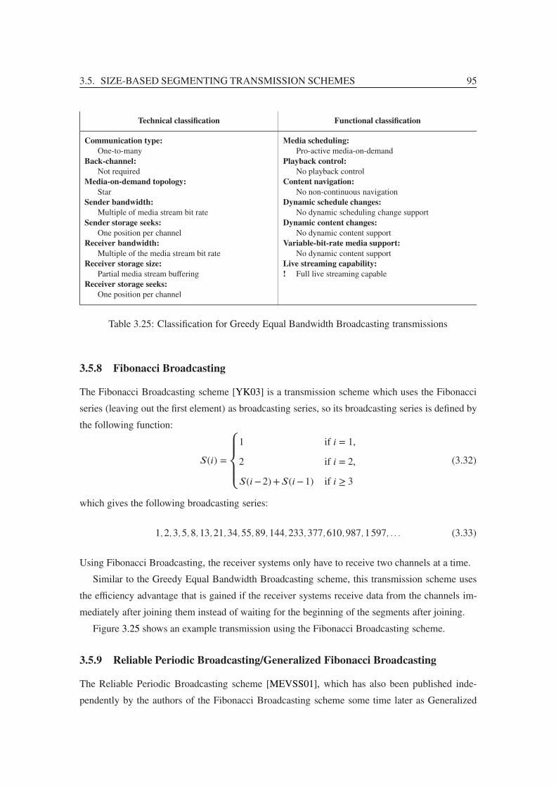
3.5. SIZE-BASED SEGMENTING TRANSMISSION SCHEMES 95
Technical classification Functional classification
Communication type:
One-to-manyBack-channel:
Not requiredMedia-on-demand topology:
StarSender bandwidth:
Multiple of media stream bit rateSender storage seeks:
One position per channelReceiver bandwidth:
Multiple of the media stream bit rateReceiver storage size:
Partial media stream bufferingReceiver storage seeks:
One position per channel
Media scheduling:
Pro-active media-on-demandPlayback control:
No playback controlContent navigation:
No non-continuous navigationDynamic schedule changes:
No dynamic scheduling change supportDynamic content changes:
No dynamic content supportVariable-bit-rate media support:
No dynamic content supportLive streaming capability:
! Full live streaming capable
Table 3.25: Classification for Greedy Equal Bandwidth Broadcasting transmissions
3.5.8 Fibonacci Broadcasting
The Fibonacci Broadcasting scheme [YK03] is a transmission scheme which uses the Fibonacci
series (leaving out the first element) as broadcasting series, so its broadcasting series is defined by
the following function:
S(i) =
⎧⎪⎪⎪⎨⎪⎪⎪⎩
1 if i = 1,
2 if i = 2,
S(i−2)+S(i−1) if i ≥ 3
(3.32)
which gives the following broadcasting series:
1,2,3,5,8,13,21,34,55,89,144,233,377,610,987,1597, . . . (3.33)
Using Fibonacci Broadcasting, the receiver systems only have to receive two channels at a time.
Similar to the Greedy Equal Bandwidth Broadcasting scheme, this transmission scheme uses
the efficiency advantage that is gained if the receiver systems receive data from the channels im-
mediately after joining them instead of waiting for the beginning of the segments after joining.
Figure 3.25 shows an example transmission using the Fibonacci Broadcasting scheme.
3.5.9 Reliable Periodic Broadcasting/Generalized Fibonacci Broadcasting
The Reliable Periodic Broadcasting scheme [MEVSS01], which has also been published inde-
pendently by the authors of the Fibonacci Broadcasting scheme some time later as Generalized

96 CHAPTER 3. MEDIA TRANSMISSION SCHEMES
��������
4
t
Channel #1:
Channel #2:
Channel #3:
Channel #4:
Channel #5: 5
4 4 4 4
5 5
1
3
2
1 1 1 1 1
2 2
3
1
3
2
1 1 1 1 1
2 2
3
1
3
2
1 1 1 1 1
2 2
3
1
3
2
1
Recipient: 1 2 3 5
Figure 3.25: Fibonacci Broadcasting
Technical classification Functional classification
Communication type:
One-to-manyBack-channel:
Not requiredMedia-on-demand topology:
StarSender bandwidth:
Multiple of media stream bit rateSender storage seeks:
One position per channelReceiver bandwidth:
! Twice the media stream bit rateReceiver storage size:
Partial media stream bufferingReceiver storage seeks:
One position per channel
Media scheduling:
Pro-active media-on-demandPlayback control:
No playback controlContent navigation:
No non-continuous navigationDynamic schedule changes:
No dynamic scheduling change supportDynamic content changes:
No dynamic content supportVariable-bit-rate media support:
No dynamic content supportLive streaming capability:
! Full live streaming capable
Table 3.26: Classification for Fibonacci Broadcasting transmissions
Fibonacci Broadcasting scheme [YK03], can be seen as a successor of the Fibonacci Broadcast-
ing scheme. Compared to the Fibonacci Broadcasting scheme, it has been generalized in such a
way that the channel bandwidth and the number of channels a receiver system is able to receive
simultaneously can be configured.
The broadcasting series of the Reliable Periodic Broadcasting scheme/Generalized Fibonacci
Broadcasting scheme can be determined from the following formula:
S(i) =
⎧⎪⎪⎪⎪⎪⎪⎪⎨⎪⎪⎪⎪⎪⎪⎪⎩
1+
i−1∑k=1
S(k)
gif i ≤R,
i−1∑k=i−R
S(k)
gif i > R
(3.34)

3.5. SIZE-BASED SEGMENTING TRANSMISSION SCHEMES 97
where g is a parameter which specifies the bandwidth of the transmission channels, i. e. the band-
width of the channels is 1g
times the media bit rate.
For g = 1 (for better comparison), this gives the following broadcasting series:
R = 2 : 1,2,3,5,8,13,21,34,55,89,144,233,377,610,987,1597,2584, . . .
R = 3 : 1,2,4,7,13,24,44,81,149,274,504,927,1705,3136,5768,10609, . . .
R = 4 : 1,2,4,8,15,29,56,108,208,401,773,1490,2872,5536,10671,20569, . . .
R = 5 : 1,2,4,8,16,31,61,120,236,464,912,1793,3525,6930,13624,26784, . . .
(3.35)
As one can see, g = 1 and R = 2 gives the broadcasting series of the Fibonacci Broadcasting
scheme and g = 1 and R =∞ gives the broadcasting series of the Greedy Equal Bandwidth Broad-
casting scheme.
Again, this transmission scheme requires that the receiver systems receive data from the chan-
nels immediately after joining them.
Figure 3.26 shows an example transmission using the Reliable Periodic Broadcasting
scheme/Generalized Fibonacci Broadcasting scheme using channels of half the media bit rate
and a receiver bandwidth of three channels (g = 2, R = 3).
1
22
3 3
4 4
5 5Channel #5:
Recipient: 1
t
2 3 4
Channel #1:
Channel #2:
Channel #3:
Channel #4:
1 1 1 1
2
Figure 3.26: Reliable Periodic Broadcasting/Generalized Fibonacci Broadcasting
3.5.10 Comparison of Size-Based Segmenting Transmission Schemes
Comparing all size-based transmission schemes with each other is very difficult as the transmission
schemes differ in several points:
• The number of channels which have to be received simultaneously by the client systems
are not the same for all transmission schemes: For Pyramid Broadcasting and Permutation-
based Pyramid Broadcasting, just one channel has to be received at once, for Skyscraper
Broadcasting and Fibonacci Broadcasting, two channels must be received in parallel, for
Mayan Temple Broadcasting and Greedy Equal Bandwidth Broadcasting, all channels have

98 CHAPTER 3. MEDIA TRANSMISSION SCHEMES
Technical classification Functional classification
Communication type:
One-to-manyBack-channel:
Not requiredMedia-on-demand topology:
StarSender bandwidth:
Multiple of media stream bit rateSender storage seeks:
One position per channelReceiver bandwidth:
! Configurable multiple of the media stream bit rateReceiver storage size:
Partial media stream bufferingReceiver storage seeks:
One position per channel
Media scheduling:
Pro-active media-on-demandPlayback control:
No playback controlContent navigation:
No non-continuous navigationDynamic schedule changes:
No dynamic scheduling change supportDynamic content changes:
No dynamic content supportVariable-bit-rate media support:
No dynamic content supportLive streaming capability:
! Full live streaming capable
Table 3.27: Classification for Reliable Periodic Broadcasting/Generalized Fibonaccy Broadcastingtransmissions
to be received simultaneously and using the Client-Centric Approach, the Greedy Disk-
Conserving Broadcasting or the Reliable Periodic Broadcasting/Generalized Fibonacci
Broadcasting, it is possible to specify the number of receiver channels.
• For the Pyramid Broadcasting and the Permutation-based Pyramid Broadcasting scheme,
the bandwidth of the channels is higher than the media bit rate while all other transmission
schemes allow using a channel bandwidth equal to the media bit rate. The Mayan Temple
Broadcasting scheme and the Reliable Periodic Broadcasting/Generalized Fibonacci Broad-
casting scheme even allow specifying a channel bandwidth independent of the media stream
bit rate.
• The Mayan Temple Broadcasting scheme supports variable-bit-rate media streams, all other
transmission schemes only support constant-bit-rate media streams.
• The Skyscraper Broadcasting scheme and the Mayan Temple Broadcasting scheme allow
specifying a limit for the required storage of the receiver system.
• The Mayan Temple Broadcasting scheme supports partial preloading.
• The Greedy Equal Bandwidth Broadcasting scheme allows defining the playback delay in-
dependent of the size of the first segment.
To get an overview of the efficiency of all size-based transmission schemes, most of these features
have to be ignored and only a few setups are examined: In a first setup, the receiver system can
only receive two channels equal to the media bit rate, while in a second setup, no limit is imposed
on the receiver bandwidth. To include Pyramid Broadcasting and Permutation-based Pyramid

3.6. BANDWIDTH-BASED SEGMENTING TRANSMISSION SCHEMES 99
Broadcasting in this comparison, a special setup is examined where the receiver system is allowed
to receive a channel of a bandwidth higher than the media bit rate11. In all setups, the receiver
storage is pretended to be sufficiently large and neither partial preloading nor variable-bit-rate
media streams are used in any of the setups. Additionally, a minimum segment size of 17200 of the
media stream size is assumed to limit splitting of the media stream.
Figures 3.27 to 3.29 show the results for each of the three setups, resp.12 For the two-channel
setup (see figure 3.27), the Reliable Periodic Broadcasting/Generalized Fibonacci Broadcasting
scheme performs best if it is used with high parameter g. The reason for this is that the Reliable
Periodic Broadcasting/Generalized Fibonacci Broadcasting scheme allows increasing the number
of segments independent from the sender and receiver bandwidth which allows approximating
the transmission frequency of the transmitted parts more exactly near to the theoretically needed
frequency. For g = 1, the Reliable Periodic Broadcasting/Generalized Fibonacci Broadcasting
scheme is identical to the Fibonacci Broadcasting scheme.
If the receiver system is able to receive the complete transmission at once (see fig-
ure 3.28), the Greedy Equal Bandwidth Broadcasting scheme and the Reliable Periodic Broad-
casting/Generalized Fibonacci Broadcasting scheme produce the same results (if the channel band-
width of the Greedy Equal Bandwidth Broadcasting scheme is set to 1g
of the media stream bit rate
where g is the parameter of the Reliable Periodic Broadcasting/Generalized Fibonacci Broadcast-
ing scheme). The Greedy Disk Conserving Bandwidth scheme and the Client Centric Approach
deliver the same results as the Greedy Equal Bandwidth Broadcasting scheme and the Reliable
Periodic Broadcasting/Generalized Fibonacci Broadcasting scheme with g = 1.
From figure 3.29 it is clearly visible that the Pyramid Broadcasting scheme and the
Permutation-based Pyramid Broadcasting scheme perform much worse than the other size-based
schemes. Please note that these schemes use integer arithmetic to calculate some of their parame-
ters which results in several lines in the efficiency graph. As the parameters are not a direct result
of the playback delay, several parameters are even valid for some playback delay values.
3.6 Bandwidth-Based Segmenting Transmission Schemes
In the previous section, the size-based transmission schemes improved the efficiency of the media-
on-demand transmissions by increasing the size of later segments and therefore reducing the trans-
mission frequency of these segments. The bandwidth-based transmission schemes use another
11The channel bandwidth of Pyramid Broadcasting and Permutation-based Pyramid Broadcasting varies dependingon the total bandwidth and the calculated α-parameter. As the efficiency values of both the Pyramid Broadcastingscheme and the Permutation-based Pyramid Broadcasting scheme are very poor, this is not examined in more detail inthis thesis.
12Please note that some of the graphs have been truncated because the segments became smaller than 17200 of the
media stream duration.

100 CHAPTER 3. MEDIA TRANSMISSION SCHEMES
10%
20%
30%
40%
50%
60%
70%
80%
90%
100%
0.0002 0.0005 0.001 0.002 0.005 0.01 0.02 0.05 0.1 0.2
Ban
dwid
th e
ffic
ienc
y
Playback delay as fraction of media stream duration
Reliable Periodic Broadcasting/Generalized Fibonacci Broadcasting (g=10)Reliable Periodic Broadcasting/Generalized Fibonacci Broadcasting (g=5)Reliable Periodic Broadcasting/Generalized Fibonacci Broadcasting (g=2)Reliable Periodic Broadcasting/Generalized Fibonacci Broadcasting (g=1)
Fibonacci BroadcastingGreedy Disk Conserving Broadcasting
Client Centric ApproachSkyscraper Broadcasting
Figure 3.27: Efficiency of size-based schemes when only twice the media bit rate can be received
10%
20%
30%
40%
50%
60%
70%
80%
90%
100%
0.0002 0.0005 0.001 0.002 0.005 0.01 0.02 0.05 0.1 0.2
Ban
dwid
th e
ffic
ienc
y
Playback delay as fraction of media stream duration
Greedy Equal Bandwidth Broadcasting (g=10)Reliable Periodic Broadcasting/Generalized Fibonacci Broadcasting (g=10)
Greedy Equal Bandwidth Broadcasting (g=3)Reliable Periodic Broadcasting/Generalized Fibonacci Broadcasting (g=3)
Greedy Equal Bandwidth Broadcasting (g=1)Reliable Periodic Broadcasting/Generalized Fibonacci Broadcasting (g=1)
Greedy Disk Conserving BroadcastingClient Centric Approach
Figure 3.28: Efficiency of size-based schemes when the whole transmission can be received atonce
approach to achieve a similar effect: Similar to the size-based transmission schemes, they use one
channel for the transmission of each segment, but instead of increasing the segment sizes for later
segments, segments of equal size are used and the bandwidth of the channels is decreased. The

3.6. BANDWIDTH-BASED SEGMENTING TRANSMISSION SCHEMES 101
10%
20%
30%
40%
50%
60%
70%
80%
90%
100%
0.0002 0.0005 0.001 0.002 0.005 0.01 0.02 0.05 0.1 0.2
Ban
dwid
th e
ffic
ienc
y
Playback delay as fraction of media stream duration
Pyramid Broadcasting (Var. a)Pyramid Broadcasting (Var. b)
Permutation-Based Pyramid Broadcasting (Var. a)Permutation-Based Pyramid Broadcasting (Var. b)
Figure 3.29: Efficiency of size-based schemes where the receiver has to receive two high-bandwidth channels
result of this bandwidth modification is that later segments take longer to be transmitted, so their
transmission frequency is lowered this way.
The remainder of this section describes transmission schemes which benefit from this approach.
The first published scheme of this class is especially interesting as it supplies some mathemati-
cal background for the calculation of a lower bound for on-demand transmissions, although the
scheme is not functional (as proven in [PCL98b]). It is followed by a series of transmission
schemes which correct this problem in different ways or focus on some other issues.
3.6.1 Harmonic Broadcasting
The Harmonic Broadcasting scheme [JT97a] uses segments of equal size and a very simple for-
mula for the bandwidth of the channels on which the segments are transmitted:
Bi =b
i(3.36)
Figure 3.30 shows an example transmission using the Harmonic Broadcasting scheme.
The idea behind this simple formula is that segment i can be transmitted at one i-th of the
media bit rate because the receiver system has i times the duration of the first segment to receive
segment #i before it is needed for playback.
The above formula assures that the segment start is received when the playback time of the

102 CHAPTER 3. MEDIA TRANSMISSION SCHEMES
5
t
Channel #1:
Recipient:
Channel #2:
Channel #3:
Channel #4:
Channel #5:
4
5 5
4 4 4 4
5 5
1
2
3 3
2 2
1 1 1 1 1 1
2
3 3
2 2
1 1 1 1 1 1
2
3 3
2 2
1 1 1 1 1 1 1
2
3
1 2 3 4
Figure 3.30: Harmonic Broadcasting
segment is reached and that the segment has been completely received when its playback time
ends. But unfortunately, this does not ensure that the segment can be played as is illustrated in
figure 3.31, a problem which results from the fact that the channel bandwidth is lower than the
media bit rate. A simple way to correct this problem is to double the playback waiting time at the
receiver side, but this decreases the efficiency of the transmission scheme a lot. In the following
subsections, other solutions are proposed.
41 2 3 5
t
Channel #1:
Recipient:
Channel #2:
Channel #3:
Channel #4:
Channel #5: 5
4 4
5 5 5
4 4 4
1 1 1 1
2 2 2
1 1
3 3
1 1 1 1
2 2 2
1 1
3 3
1 1 1 1
2 2 2
1 1
3 3
1 1
2
3
Figure 3.31: Example for failure of Harmonic Broadcasting: The blackened parts at the recipientare missing when the media stream is played
Although this means that the transmission scheme is non-functional, it marks a very important
step in the evolution of transmission schemes as it introduced a new and very efficient class of
transmission schemes.
3.6.2 Cautious Harmonic Broadcasting
The authors of [PCL98b] not only discovered that the Harmonic Broadcasting Protocol is not
working in the proposed version, they also provided three broadcasting schemes as solutions which
are presented in this and the following two subsections.
The Cautious Harmonic Broadcasting scheme [PCL98b] is one of their solutions. For this
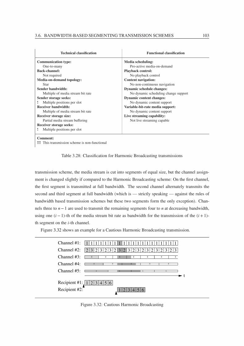
3.6. BANDWIDTH-BASED SEGMENTING TRANSMISSION SCHEMES 103
Technical classification Functional classification
Communication type:
One-to-manyBack-channel:
Not requiredMedia-on-demand topology:
StarSender bandwidth:
Multiple of media stream bit rateSender storage seeks:
! Multiple positions per slotReceiver bandwidth:
Multiple of media stream bit rateReceiver storage size:
Partial media stream bufferingReceiver storage seeks:
! Multiple positions per slot
Media scheduling:
Pro-active media-on-demandPlayback control:
No playback controlContent navigation:
No non-continuous navigationDynamic schedule changes:
No dynamic scheduling change supportDynamic content changes:
No dynamic content supportVariable-bit-rate media support:
No dynamic content supportLive streaming capability:
Not live streaming capable
Comment:
!!! This transmission scheme is non-functional
Table 3.28: Classification for Harmonic Broadcasting transmissions
transmission scheme, the media stream is cut into segments of equal size, but the channel assign-
ment is changed slightly if compared to the Harmonic Broadcasting scheme: On the first channel,
the first segment is transmitted at full bandwidth. The second channel alternately transmits the
second and third segment at full bandwidth (which is — strictly speaking — against the rules of
bandwidth based transmission schemes but these two segments form the only exception). Chan-
nels three to n−1 are used to transmit the remaining segments four to n at decreasing bandwidth,
using one (i− 1)-th of the media stream bit rate as bandwidth for the transmission of the (i+ 1)-
th segment on the i-th channel.
Figure 3.32 shows an example for a Cautious Harmonic Broadcasting transmission.
6
Channel #1:
Recipient #1:
Channel #2:
Channel #3:
Channel #4:
Channel #5:
Recipient #2:
t
11 1 1 11 1 1 11 1 1 11 1 1 11 1 1
2 2 2 2 2 2 2 2 2 2
1 2 3 4 5
1 2 3 4 5
3 3 3 3 3 3 3 3 3
6
6
34 4 4 4 4 4 4
5 5 5 5 5
6 6 6
Figure 3.32: Cautious Harmonic Broadcasting

104 CHAPTER 3. MEDIA TRANSMISSION SCHEMES
Technical classification Functional classification
Communication type:
One-to-manyBack-channel:
Not requiredMedia-on-demand topology:
StarSender bandwidth:
Multiple of media stream bit rateSender storage seeks:
! Multiple positions per slotReceiver bandwidth:
Multiple of media stream bit rateReceiver storage size:
Partial media stream bufferingReceiver storage seeks:
! Multiple positions per slot
Media scheduling:
Pro-active media-on-demandPlayback control:
No playback controlContent navigation:
No non-continuous navigationDynamic schedule changes:
No dynamic scheduling change supportDynamic content changes:
No dynamic content supportVariable-bit-rate media support:
No dynamic content supportLive streaming capability:
Not live streaming capable
Table 3.29: Classification for Cautious Harmonic Broadcasting transmissions
3.6.3 Quasi-Harmonic Broadcasting
The Quasi-Harmonic Broadcasting scheme [PCL98b] is another solution to solve the problems of
the Harmonic Broadcasting Protocol.
For the Quasi-Harmonic Broadcasting scheme, the media stream is not only cut into segments
of equal size, all segments except the first one are further cut into smaller subsegments and trans-
mitted using a complex scheme:
The first segment is simply transmitted on the first channel at the full media stream bit rate.
But channel i ≥ 2 transmits all subsegments of the segment i at mi·m−1 times the media stream bit
rate in the order specified by the series
⎛⎝⎧⎨⎩i · (t mod m)+
⌊tmod im
m
⌋if t mod m �= m−1,
(t mod (i−1))+1 if t mod m = m−1
⎞⎠
t∈{0,1,2,...,i·m−1}
(3.37)
where m ≥ 2 is a parameter. The advantage of the Quasi-Harmonic Broadcasting scheme is that
it converges to the same bandwidth requirements as the non-functional Harmonic Broadcasting
scheme if m tends towards infinity. Figure 3.33 shows an example transmission for the Quasi-
Harmonic Broadcasting scheme.
3.6.4 Polyharmonic Broadcasting
The Polyharmonic Broadcasting scheme [PCL98c] uses another trick to get around the design er-
ror of Harmonic Broadcasting: Instead of starting the playback when the beginning of the first

3.6. BANDWIDTH-BASED SEGMENTING TRANSMISSION SCHEMES 105
����������
����������
����������������������������
����������7 11 15 1
10 15 1 65 11 16 2 7 1712 3 8 13 18 4 9 14 19 1
4 8 12 2
3 6 9 1 4 7 2 5 8 311 1 3 6 9 1 4 7310 310 2
4 6 1 3 5 7 12 2 4 6 1 3 5 7 1 2 4 6 1
t
Channel #1:
Recipient #1:
Channel #2:
Channel #3:
Channel #4:
Channel #5:
1 2 3 4 5
2
3
4
5
1 1 1 1 1
2 2 2 2 2 2 2 2 2 2 2 2 2 2 2 2 2 2 2
3 3 3 3 3 3 3 3 3 3 3 3 3 3 3 3
4 4 4 4 4 4 4 4 4 4 4 4 4 4 4 4 4 4 4
5 5 5 5 5 5 5 5 5 5 5 5 5 5 5 5 5 5 5
4 8 12 1 2 35 9 13 6 10 14
Figure 3.33: Quasi-Harmonic Broadcasting with parameter m = 4
Technical classification Functional classification
Communication type:
One-to-manyBack-channel:
Not requiredMedia-on-demand topology:
StarSender bandwidth:
Multiple of media stream bit rateSender storage seeks:
! Multiple positions per slotReceiver bandwidth:
Multiple of media stream bit rateReceiver storage size:
Partial media stream bufferingReceiver storage seeks:
! Multiple positions per slot
Media scheduling:
Pro-active media-on-demandPlayback control:
No playback controlContent navigation:
No non-continuous navigationDynamic schedule changes:
No dynamic scheduling change supportDynamic content changes:
No dynamic content supportVariable-bit-rate media support:
No dynamic content supportLive streaming capability:
Not live streaming capable
Table 3.30: Classification for Quasi-Harmonic Broadcasting transmissions
segment is received (and therefore the next slot interval boundary is reached), Polyharmonic
Broadcasting uses the fixed wait policy which already has been presented in section 3.5.7 for
the Greedy Equal Bandwidth Broadcasting scheme, i. e. segments are received immediately after
joining the channel (instead of waiting for the next segment boundary when joining) and the play-
back is started a fixed time after the receiver system started reception (and not at the next segment
boundary). This way, Polyharmonic Broadcasting assures that each segment has been completely
received when its playback is started.
As the bandwidth division and segment mapping are the same as of Harmonic Broadcasting,
Polyharmonic Broadcasting reaches the bandwidth promises of Harmonic Broadcasting. The only
difference is that the minimum playback delay equals the maximum playback delay for the Poly-
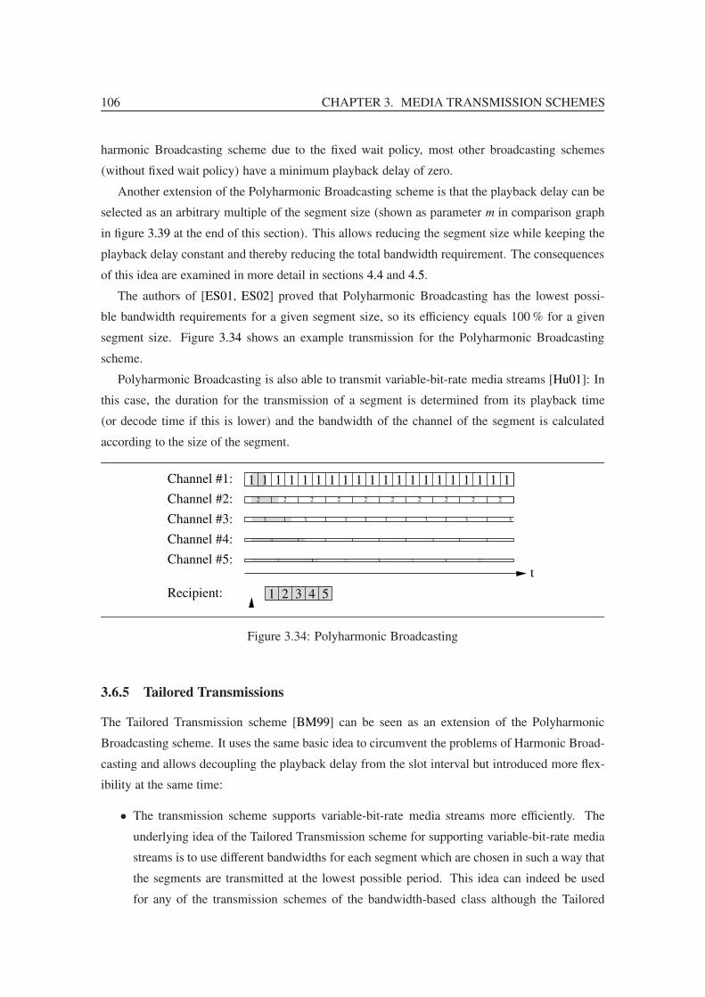
106 CHAPTER 3. MEDIA TRANSMISSION SCHEMES
harmonic Broadcasting scheme due to the fixed wait policy, most other broadcasting schemes
(without fixed wait policy) have a minimum playback delay of zero.
Another extension of the Polyharmonic Broadcasting scheme is that the playback delay can be
selected as an arbitrary multiple of the segment size (shown as parameter m in comparison graph
in figure 3.39 at the end of this section). This allows reducing the segment size while keeping the
playback delay constant and thereby reducing the total bandwidth requirement. The consequences
of this idea are examined in more detail in sections 4.4 and 4.5.
The authors of [ES01, ES02] proved that Polyharmonic Broadcasting has the lowest possi-
ble bandwidth requirements for a given segment size, so its efficiency equals 100 % for a given
segment size. Figure 3.34 shows an example transmission for the Polyharmonic Broadcasting
scheme.
Polyharmonic Broadcasting is also able to transmit variable-bit-rate media streams [Hu01]: In
this case, the duration for the transmission of a segment is determined from its playback time
(or decode time if this is lower) and the bandwidth of the channel of the segment is calculated
according to the size of the segment.
3����
t
Channel #1:
Recipient:
Channel #2:
Channel #3:
Channel #4:
Channel #5: 5
4 4 4 4
5 5 5
1
3
2
1 1 1 1 12 2
3
1
3
2
1 1 1 1 12 2
3
1
3
2
1 1 12
3
1 2 3 4 5
1 12
1 12
4
����
Figure 3.34: Polyharmonic Broadcasting
3.6.5 Tailored Transmissions
The Tailored Transmission scheme [BM99] can be seen as an extension of the Polyharmonic
Broadcasting scheme. It uses the same basic idea to circumvent the problems of Harmonic Broad-
casting and allows decoupling the playback delay from the slot interval but introduced more flex-
ibility at the same time:
• The transmission scheme supports variable-bit-rate media streams more efficiently. The
underlying idea of the Tailored Transmission scheme for supporting variable-bit-rate media
streams is to use different bandwidths for each segment which are chosen in such a way that
the segments are transmitted at the lowest possible period. This idea can indeed be used
for any of the transmission schemes of the bandwidth-based class although the Tailored

3.6. BANDWIDTH-BASED SEGMENTING TRANSMISSION SCHEMES 107
Technical classification Functional classification
Communication type:
One-to-manyBack-channel:
Not requiredMedia-on-demand topology:
StarSender bandwidth:
Multiple of media stream bit rateSender storage seeks:
! Multiple positions per slotReceiver bandwidth:
Multiple of media stream bit rateReceiver storage size:
Partial media stream bufferingReceiver storage seeks:
! Multiple positions per slot
Media scheduling:
Pro-active media-on-demandPlayback control:
No playback controlContent navigation:
No non-continuous navigationDynamic schedule changes:
No dynamic scheduling change supportDynamic content changes:
No dynamic content supportVariable-bit-rate media support:
No dynamic content supportLive streaming capability:
Not live streaming capable
Table 3.31: Classification for Polyharmonic Broadcasting transmissions
Transmission scheme is the only one which describes this approach. Further information on
variable-bit-rate transmissions is given in section 4.8.
• The transmission scheme allows selecting all but one of the design parameters media length,
playback delay, receiver bandwidth, transmission bandwidth and receiver storage require-
ments and throughput to create a matching transmission scheme.
Technical classification Functional classification
Communication type:
One-to-manyBack-channel:
Not requiredMedia-on-demand topology:
StarSender bandwidth:
Multiple of media stream bit rateSender storage seeks:
! Multiple positions per slotReceiver bandwidth:
Multiple of media stream bit rateReceiver storage size:
Partial media stream bufferingReceiver storage seeks:
! Multiple positions per slot
Media scheduling:
Pro-active media-on-demandPlayback control:
No playback controlContent navigation:
No non-continuous navigationDynamic schedule changes:
No dynamic scheduling change supportDynamic content changes:
No dynamic content supportVariable-bit-rate media support:
No dynamic content supportLive streaming capability:
Not live streaming capable
Table 3.32: Classification for Tailored Broadcasting transmissions

108 CHAPTER 3. MEDIA TRANSMISSION SCHEMES
3.6.6 Staircase Broadcasting
The Staircase Broadcasting scheme [JT97b] is another transmission scheme of the class of
bandwidth-based transmission schemes. In contrary to the above ones, it is based on a binary
splitting of the bandwidth, i. e. segments #2k to #2k+1 − 1 are transmitted at 12k
of the media bit
rate (k ≥ 0). As a result, the channels of the transmission can be aggregated into channels at media
bit rate.
3 4
21 22
41
51 52
42 43
53 54
44
3231
Recipient: 141424344
313222
21
54535251
64636261
74737271
t
11 1 1 1 1 1 1 1 1
Channel #7:Channel #6:Channel #5:Channel #4:
Channel #3:
Channel #2:
Channel #1:
2 21 22 21 22 21 22 21 2
3 31 23 31 2 3 31 2 3 31 2
4 41 24 41 2 4 43 4
5 51 25 51 2 5 53 4
6 61 26 61 2 6 63 46 61 2 6 63 4
7 71 27 71 2 7 73 4 7 71 2 7 7
Figure 3.35: Staircase Broadcasting
To circumvent the problems of Harmonic Broadcasting, the authors of the Staircase Broadcast-
ing scheme used another type of subsegment splitting: Instead of splitting a segment into sub-
segments of same duration to transmit them on low bandwidth channels (vertical partitioning),
they split the segment transmission into streams of same bandwidth (horizontal partitioning).
This allows playing a segment even when the first subsegment is just received — which was the
problem of Harmonic Broadcasting. Figure 3.35 shows an example for a Staircase Broadcasting
transmission and figure 3.36 shows the difference between vertical and horizontal partitioning for
a two segment transmission.
Although this splitting technique seems to be a completely new idea, it has already been pro-
posed similarly in a previous transmission scheme. To understand this, it is important to realize
that transmitting a segment in streams of same bandwidth has to be performed by splitting it into
small parts which are interleaved for transmission. But this introduces an additional, small play-
back delay as the first part of the first subsegment has to be played at full speed while it is received
with lower bandwidth. This problem can be solved if the first parts of the first subsegments of
the segments are transmitted more often. Exactly this approach is used in the Quasi-Harmonic
Broadcasting scheme, where the parameter m describes in how many parts a subsegment is split.

3.6. BANDWIDTH-BASED SEGMENTING TRANSMISSION SCHEMES 109
��������1
221 2
1
21
1 1 1 1
2 212
t
Channel #1:
Recipient:
Channel #2:
1
22 2
(a) Subsegments of same duration produce problems atHarmonic Broadcasting
��������
21
21
22
1
21
1 1 1 1
2 212
t
Channel #1:
Recipient:
Channel #2:
1
22
(b) Subsegments of same bandwidth can be used for in-stead
Figure 3.36: Comparison of different sub-segmentation schemes
Technical classification Functional classification
Communication type:
One-to-manyBack-channel:
Not requiredMedia-on-demand topology:
StarSender bandwidth:
Multiple of media stream bit rateSender storage seeks:
! Multiple positions per slotReceiver bandwidth:
Multiple of media stream bit rateReceiver storage size:
Partial media stream bufferingReceiver storage seeks:
! Multiple positions per slot
Media scheduling:
Pro-active media-on-demandPlayback control:
No playback controlContent navigation:
No non-continuous navigationDynamic schedule changes:
No dynamic scheduling change supportDynamic content changes:
No dynamic content supportVariable-bit-rate media support:
No dynamic content supportLive streaming capability:
Not live streaming capable
Table 3.33: Classification for Staircase Broadcasting transmissions
3.6.7 Seamless Staircase Broadcasting
The Seamless Staircase Broadcasting scheme [TCS04] has a very similar structure as the Staircase
Broadcasting scheme which has been proposed in the previous subsection. Similar to the Staircase
Broadcasting scheme, the segments are transmitted for this transmission scheme in such a way that
the channels can be aggregated into channels at media bit rate.
The main difference between the Seamless Staircase Broadcasting scheme and the Staircase
Broadcasting scheme is that the Seamless Staircase Broadcasting scheme does not use the binary
horizontal partitioning scheme for the first three channels. Instead, the following schedule is used:
• The first segment is transmitted at media bit rate.
• The second and third segment are transmitted at media bit rate alternately.
• Segment #3 ·2k +1 to #3 ·2k+1 are transmitted at 13·2k of the media bit rate (k ≥ 0).
Figure 3.37 shows an example for a Seamless Staircase Broadcasting transmission.
Although this transmission scheme is less efficient than the original Staircase Broadcasting

110 CHAPTER 3. MEDIA TRANSMISSION SCHEMES
1 62 63 61 62 63 6161 62 63
1Recipient: 2 3 42 52 6
4
2
1 51 61
643 53 3
51 52 53 51 52 53 5151 52 53Channel #4−6:
t
2 3 2 3 2 3 2 3 2 3Channel #2+3:
Channel #1: 11 1 1 1 1 1 1 1 1
41 42 43 41 42 43 4141 42 43
6
Figure 3.37: Seamless Staircase Broadcasting
scheme, the Seamless Staircase Broadcasting scheme can be regarded as an enhanced version
of the former one as it supports a seamless bandwidth change: Often the media-on-demand
providers want be able to change the bandwidth assignments to media streams to increase or
decrease the playback delay dynamically. As ongoing transmissions should not be disrupted, the
only chance to perform these changes for most transmission schemes is to start the transmission
with the new parameters in parallel to the ongoing one and “fading out” the old transmission. The
disadvantage of this procedure is that both transmissions consume bandwidth during the transition
time.
With the Seamless Staircase Broadcasting scheme, the bandwidth can be increased dynamically
(in steps of the media bit rate): Each time the bandwidth is increased by the media bit rate, the
playback delay halves a short time thereafter13. It is even possible to double the playback delay at
a later time up to the initial value, thereby releasing bandwidth again after the transition finished.
Figure 3.38 shows an example where bandwidth is dynamically added, including an ongoing
playback (recipient #1 in the figure) which continues uninterrupted after the bandwidth change and
a playback (recipient #2) which is served after the bandwidth has been changed. Seamless band-
width changes are re-examined in section 4.16 as an extension to the newly proposed Generalized
Greedy Broadcasting scheme.
13Unfortunately, the Seamless Staircase Broadcasting scheme cannot serve playback requests while this transitiontakes place, a fact which has not been mentioned by the authors of the transmission scheme.

3.6. BANDWIDTH-BASED SEGMENTING TRANSMISSION SCHEMES 111
2D5 5
553A5 5
3D55
1C1D1B
1A55
55
2A2B
2C2D
5 555
3A3B
3C5 53D55
1D1A6 6
6 62A
2D66 6
6 3A66 3D6
6
2A2B
2C2D
66 6
6
1C1D1B
1A6 66 6
3A3B
3C66 3D6
6
2A2D
66 6
6
2A2B
2C2D
66 6
6
2B2C
3B3C
1B1C
2B2C 3C
3B1C
1B
2B 3B 1B 2B 3B 1B2C 3C 1C 2C 3C 1C
2B 3B 1B 2B 3B 1B2C 3C 1C 2C 3C 1C
Recipient #1:
Recipient #2:
t
41 42 43
51 52 53 51
61 62 63 61
2 3 2 3
11 1 1
1 3D44
44
3A4
44
42A2D 4
44
41D
1A
1D1A5
555
1D1A6 6
6 6
2A2D
3A5 5 5 53D5555
3A66 3D6
6
1B2A1B2A1B2A1B2A1B2A
1A1A1A1A1A1A1A1A1A1A1A
4
D2 B C D2 2 2 B C D2 2 2 B C2 2
3C
3F 3 3D E
3 3A B 3 3 3C A B
3 3 3D EF 3 3 3D EF
3 3 3C A B
42 52
643 53 3
41 51 61
1 2 3
1A
1A
2A1B
2A1B
2D B C2 2
3 3A B
3 3D E 3F
3C
B2
C2
2D
3B
3C
A3 3D
3E
3F
1D444
4 1C1B1A
2D444
42A2B
2C
44
43A3B
3C
1D444
41A2D4
44
42A 44
43A
3D4
3D4
1D1A5
555
2A
Figure 3.38: Seamless Staircase Broadcasting
3.6.8 Comparison of Bandwidth-Based Segmenting Transmission Schemes
Comparing all bandwidth-based segmenting transmission schemes with each other imposes simi-
lar difficulties as the comparison of the size-based segmenting transmissions schemes:
• The Quasi-Harmonic Broadcasting scheme, the Polyharmonic Broadcasting scheme and the
Tailored Transmission scheme support a parameter14, which, if set to a high value, increases
the efficiency. For the Polyharmonic Broadcasting scheme and the Tailored Transmission
scheme, the efficiency even tends towards 100 % if the parameter is increased indefinitely.
(But as this also increases the number of segments, calculations are stopped when the trans-
mission scheme uses more segments than the lower bound bandwidth calculation assumed,
otherwise the efficiency of these transmission schemes would advance beyond 100 % be-
cause of the smaller segment sizes.)
• The Polyharmonic Broadcast scheme and the Tailored Transmission scheme also supports
14In the original article of the Tailored Transmission scheme, the ratio of playback delay to segment size has not beennamed. As the Tailored Transmission scheme can be seen as an extension of the Polyharmonic Broadcasting scheme,
the same parameter definition m = W +
δis used in this thesis.

112 CHAPTER 3. MEDIA TRANSMISSION SCHEMES
Technical classification Functional classification
Communication type:
One-to-manyBack-channel:
Not requiredMedia-on-demand topology:
StarSender bandwidth:
Multiple of media stream bit rateSender storage seeks:
! Multiple positions per slotReceiver bandwidth:
Multiple of media stream bit rateReceiver storage size:
Partial media stream bufferingReceiver storage seeks:
! Multiple positions per slot
Media scheduling:
Pro-active media-on-demandPlayback control:
No playback controlContent navigation:
No non-continuous navigationDynamic schedule changes:
! Full dynamic scheduling change supportDynamic content changes:
No dynamic content supportVariable-bit-rate media support:
No dynamic content supportLive streaming capability:
Not live streaming capable
Comment:
!!! No playback requests can be processed during bandwidth change
Table 3.34: Classification for Seamless Staircase Broadcasting transmissions
variable-bit-rate media streams and allows restricting the receiver bandwidth, receiver stor-
age size and throughput.
• The Seamless Staircase Broadcasting scheme supports seamless bandwidth changes for on-
going transmissions.
• For the Polyharmonic Broadcasting scheme and the Tailored Transmission scheme, the
minimum playback delay equals the maximum playback delay, for the other transmission
schemes of the bandwidth based group, the minimum playback delay is zero.
To compare the bandwidth-based transmission schemes, the following assumptions have been
made:
• The bandwidth of the receiver systems is high enough to receive any of the transmissions.
• The storage space available at the receiver systems and the throughput of it are high enough
to cope with the transmission.
• A constant-bit-rate media stream is transmitted.
• Only the maximum playback delay is taken into account when the efficiency is calculated.
Under these preconditions, figure 3.39 shows the efficiency of the bandwidth-based transmission
schemes. (The Harmonic Broadcasting scheme has been omitted as it is not working correctly, see
section 3.6.1.) It is clearly visible, that the Polyharmonic Broadcasting scheme and the Tailored

3.7. FREQUENCY-BASED SEGMENTING TRANSMISSION SCHEMES 113
Transmission scheme (which produce identical results under the above preconditions) outperform
the other bandwidth-based transmission schemes.
10%
20%
30%
40%
50%
60%
70%
80%
90%
100%
0.0002 0.0005 0.001 0.002 0.005 0.01 0.02 0.05 0.1 0.2
Ban
dwid
th e
ffic
ienc
y
Playback delay as fraction of media stream duration
Polyharmonic Broadcasting (m=10)Tailored Transmissions (m=10)
Polyharmonic Broadcasting (m=3)Tailored Transmissions (m=3)
Polyharmonic Broadcasting (m=1)Tailored Transmissions (m=1)
Quasi-Harmonic Broadcasting (m=10)Quasi-Harmonic Broadcasting (m=3)Quasi-Harmonic Broadcasting (m=2)
Cautious Harmonic BroadcastingStaircase Broadcasting
Seamless Staircase Broadcasting
Figure 3.39: Efficiency of bandwidth-based schemes
3.7 Frequency-Based Segmenting Transmission Schemes
The third class of pro-active media-on-demand transmission schemes uses channels of equal band-
width where segments of equal size are transmitted. Instead of using segments of increasing size
or decreasing bandwidth, the frequency-based transmission schemes transmit the segments at de-
creasing frequency. As the average bandwidth which is used for the transmission of the segments
decreases for the later segments, bandwidth is saved.
The main advantage of this procedure is that all segments are of equal size and that all channels
use the same bandwidth. But to perform a successful frequency-based transmission, the segments
have to be arranged on the channels in such a way that no two segments of one channel have to
be transmitted at the same time. As the calculation of the optimal arrangement is NP-hard (this
problem is a variant of the bin-packing problem [Wik08g] as proven in [BNBNS98]), only non-
perfect solutions are available for large transmission schedules, so the transmission schemes which
are presented in this section mainly differ in the algorithm they use for arranging the segments.

114 CHAPTER 3. MEDIA TRANSMISSION SCHEMES
3.7.1 Harmonic Equal-Bandwidth Broadcasting
Although never published separately, this broadcasting scheme is referenced several times when
it comes to frequency-based transmission schemes. The reason therefore is that it is the most
efficient frequency-based transmission scheme: It has an efficiency of 100 %.
The Harmonic Equal-Bandwidth Broadcasting scheme uses a single channel for each segment,
each at the media stream bit rate (assuming a constant-bit-rate media stream), and the i-th seg-
ment is transmitted every i+⌊W +
δ
⌋−1 slot intervals on its channel. (Similar to the Polyharmonic
Broadcasting scheme, it is possible to use a playback delay independent from the segment size
to increase the efficiency.) Due to its similarities with the Polyharmonic Broadcasting scheme,
the Harmonic Equal-Bandwidth Broadcasting scheme reaches the same efficiency as the Polyhar-
monic Broadcasting scheme, but without the need for a fixed wait policy.
Unfortunately, the bandwidth of this transmission scheme is extremely varying: At the be-
ginning of the transmission (t = 0), only one channel transmits a segment, but at time off-
set t = δ · lcm1≤i≤n
i all n channels are in use15 which makes the transmission scheme unusable in
practical environments. Figure 3.40 shows an example for five channels.
Recipient #1:Recipient #2:
Channel #4:Channel #3:Channel #2:Channel #1:
Channel #5:
1 1 1 1 11 1 1 1 1 1 1 11 1
4 4 44 4
3 3 3 3 33
2 2 2 2 2 2 2 2 2 2
t5 5 5 5
1 2 3 54
1 2 3 54
1111 1
Figure 3.40: Harmonic Equal-Bandwidth Broadcasting
3.7.2 Fast Broadcasting
The Fast Broadcasting transmission scheme [JT98] was the first scheme which has been published
for the frequency-based class and started this new, very efficient and useful type of transmission
schemes. It uses a simple, binary scheme for the segment arrangement as illustrated in figure 3.41.
To write a frequency-based transmission scheme down, several different notations are used in
the literature. The following are the most important ones:
• As frequency-based transmission schemes are periodic, the most simple method for showing
a frequency-based transmission scheme is to enumerate the segments of one period for each
channel. Sadly, the period becomes very large for some transmission schemes, e. g. the
15The lcm operator denotes the least common multiple.
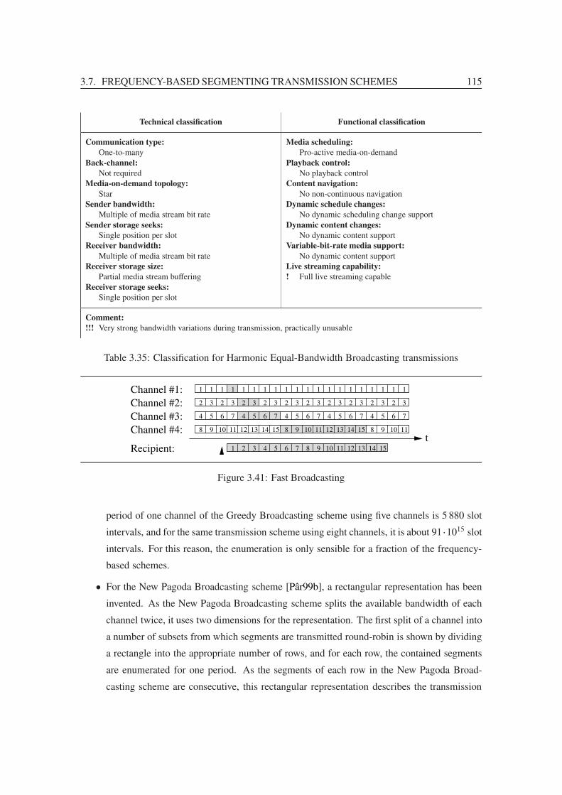
3.7. FREQUENCY-BASED SEGMENTING TRANSMISSION SCHEMES 115
Technical classification Functional classification
Communication type:
One-to-manyBack-channel:
Not requiredMedia-on-demand topology:
StarSender bandwidth:
Multiple of media stream bit rateSender storage seeks:
Single position per slotReceiver bandwidth:
Multiple of media stream bit rateReceiver storage size:
Partial media stream bufferingReceiver storage seeks:
Single position per slot
Media scheduling:
Pro-active media-on-demandPlayback control:
No playback controlContent navigation:
No non-continuous navigationDynamic schedule changes:
No dynamic scheduling change supportDynamic content changes:
No dynamic content supportVariable-bit-rate media support:
No dynamic content supportLive streaming capability:
! Full live streaming capable
Comment:
!!! Very strong bandwidth variations during transmission, practically unusable
Table 3.35: Classification for Harmonic Equal-Bandwidth Broadcasting transmissions
Recipient:
Channel #4:Channel #3:Channel #2:Channel #1: 1 1
32
4 5 6 7
8 9 10 11
32
1 1 1 1 1 1 11 1 1 1 1 1 1 11 1
32322 33232322 332
54 76 4 5 7654 4 5 76
8 9 11101312 1514 8 9 1110t
1312 1514
76
761 2 3 54 15148 9 1110 1312
1
Figure 3.41: Fast Broadcasting
period of one channel of the Greedy Broadcasting scheme using five channels is 5 880 slot
intervals, and for the same transmission scheme using eight channels, it is about 91 ·1015 slot
intervals. For this reason, the enumeration is only sensible for a fraction of the frequency-
based schemes.
• For the New Pagoda Broadcasting scheme [Pâr99b], a rectangular representation has been
invented. As the New Pagoda Broadcasting scheme splits the available bandwidth of each
channel twice, it uses two dimensions for the representation. The first split of a channel into
a number of subsets from which segments are transmitted round-robin is shown by dividing
a rectangle into the appropriate number of rows, and for each row, the contained segments
are enumerated for one period. As the segments of each row in the New Pagoda Broad-
casting scheme are consecutive, this rectangular representation describes the transmission
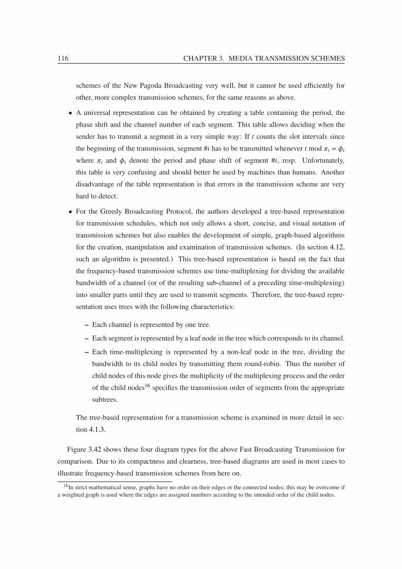
116 CHAPTER 3. MEDIA TRANSMISSION SCHEMES
schemes of the New Pagoda Broadcasting very well, but it cannot be used efficiently for
other, more complex transmission schemes, for the same reasons as above.
• A universal representation can be obtained by creating a table containing the period, the
phase shift and the channel number of each segment. This table allows deciding when the
sender has to transmit a segment in a very simple way: If t counts the slot intervals since
the beginning of the transmission, segment #i has to be transmitted whenever t mod πi = φi
where πi and φi denote the period and phase shift of segment #i, resp. Unfortunately,
this table is very confusing and should better be used by machines than humans. Another
disadvantage of the table representation is that errors in the transmission scheme are very
hard to detect.
• For the Greedy Broadcasting Protocol, the authors developed a tree-based representation
for transmission schedules, which not only allows a short, concise, and visual notation of
transmission schemes but also enables the development of simple, graph-based algorithms
for the creation, manipulation and examination of transmission schemes. (In section 4.12,
such an algorithm is presented.) This tree-based representation is based on the fact that
the frequency-based transmission schemes use time-multiplexing for dividing the available
bandwidth of a channel (or of the resulting sub-channel of a preceding time-multiplexing)
into smaller parts until they are used to transmit segments. Therefore, the tree-based repre-
sentation uses trees with the following characteristics:
– Each channel is represented by one tree.
– Each segment is represented by a leaf node in the tree which corresponds to its channel.
– Each time-multiplexing is represented by a non-leaf node in the tree, dividing the
bandwidth to its child nodes by transmitting them round-robin. Thus the number of
child nodes of this node gives the multiplicity of the multiplexing process and the order
of the child nodes16 specifies the transmission order of segments from the appropriate
subtrees.
The tree-based representation for a transmission scheme is examined in more detail in sec-
tion 4.1.3.
Figure 3.42 shows these four diagram types for the above Fast Broadcasting Transmission for
comparison. Due to its compactness and clearness, tree-based diagrams are used in most cases to
illustrate frequency-based transmission schemes from here on.
16In strict mathematical sense, graphs have no order on their edges or the connected nodes; this may be overcome ifa weighted graph is used where the edges are assigned numbers according to the intended order of the child nodes.
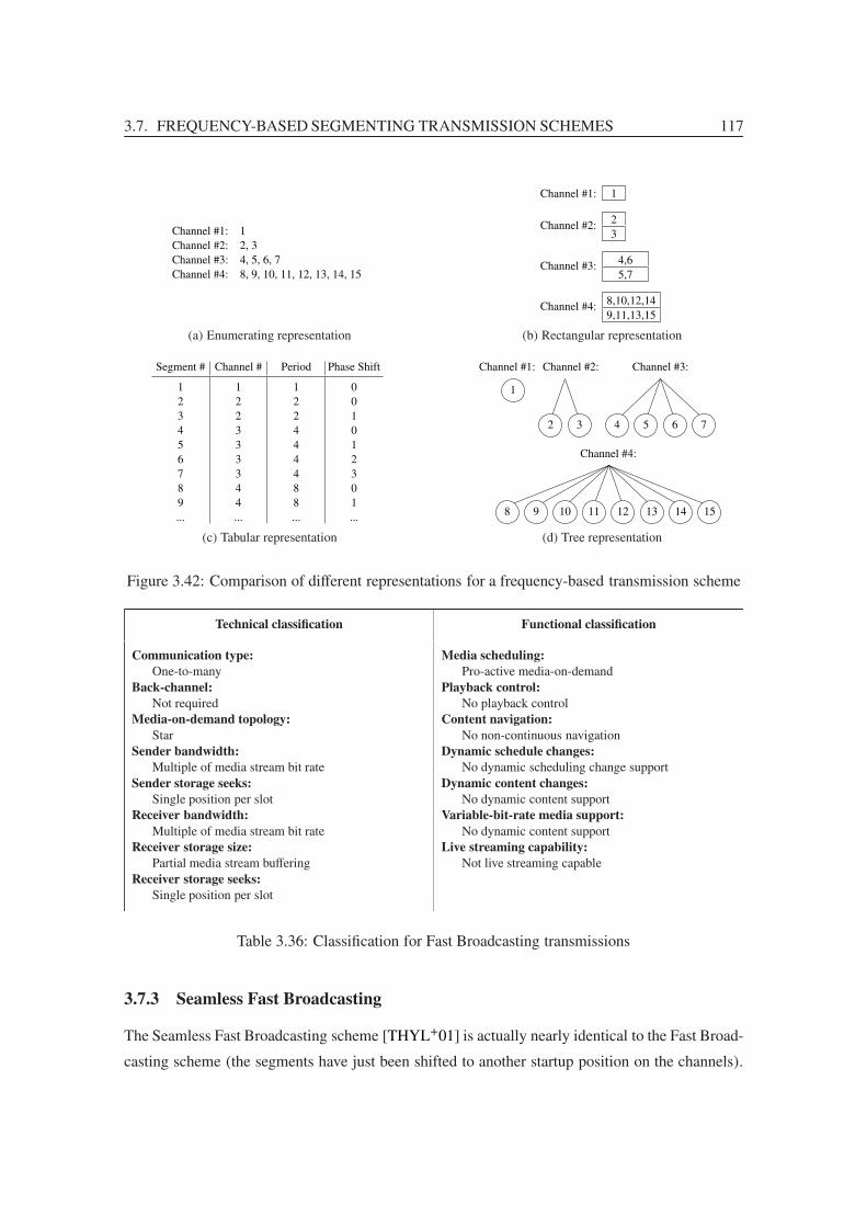
3.7. FREQUENCY-BASED SEGMENTING TRANSMISSION SCHEMES 117
8, 9, 10, 11, 12, 13, 14, 15
Channel #2:Channel #3:Channel #4:
12, 34, 5, 6, 7
Channel #1:
(a) Enumerating representation
8,10,12,149,11,13,15
23
1
Channel #2:
Channel #4:
Channel #3:
Channel #1:
5,74,6
(b) Rectangular representation
...
Channel # Period Phase ShiftSegment #
123456789...
122333344...
122444488...
001012301
(c) Tabular representation
Channel #2:
Channel #4:
8 9 10 11 12 13 14 15
2 3 4 5 6 7
1
Channel #3:Channel #1:
(d) Tree representation
Figure 3.42: Comparison of different representations for a frequency-based transmission scheme
Technical classification Functional classification
Communication type:
One-to-manyBack-channel:
Not requiredMedia-on-demand topology:
StarSender bandwidth:
Multiple of media stream bit rateSender storage seeks:
Single position per slotReceiver bandwidth:
Multiple of media stream bit rateReceiver storage size:
Partial media stream bufferingReceiver storage seeks:
Single position per slot
Media scheduling:
Pro-active media-on-demandPlayback control:
No playback controlContent navigation:
No non-continuous navigationDynamic schedule changes:
No dynamic scheduling change supportDynamic content changes:
No dynamic content supportVariable-bit-rate media support:
No dynamic content supportLive streaming capability:
Not live streaming capable
Table 3.36: Classification for Fast Broadcasting transmissions
3.7.3 Seamless Fast Broadcasting
The Seamless Fast Broadcasting scheme [THYL+01] is actually nearly identical to the Fast Broad-
casting scheme (the segments have just been shifted to another startup position on the channels).

118 CHAPTER 3. MEDIA TRANSMISSION SCHEMES
But similar to the Seamless Staircase Broadcasting scheme (see section 3.6.7), the Seamless Fast
Broadcasting scheme supports bandwidth changes for ongoing transmissions.
Figure 3.43 shows the process of a seamless channel addition for the Seamless Fast Broadcast-
ing scheme.
Recipient #2:
Added Ch.:Channel #1:Channel #2:Channel #3:
Recipient #1:B2 2 3 3 4 4 5 5
A B A B6 6 7 7
A B A B6 6 7 7
t
A
BA
BA
B
A
4
1
2 1
24
1
−
A
BA
BA
B
A
4
1
2 1
24
1
−
1 11 1
6 7
2 3
4
23
5
3
5
1
1 2 3 4 5
A
BA
BA BA
BA
BA
A
BA
BA
BA
A A
BA
BA
BA BA
BA
BA
AA A A A A
6 6 7 7 5 5 6 6 7 7
2
1 1 1 1 1
2 21 1 1 12 2
1 1
2 334 33 2 334
1 1A1
B1
AB1A1 B A B A B A
Figure 3.43: Example for a channel addition in an ongoing transmission using the Seamless FastBroadcasting scheme
Technical classification Functional classification
Communication type:
One-to-manyBack-channel:
Not requiredMedia-on-demand topology:
StarSender bandwidth:
Multiple of media stream bit rateSender storage seeks:
Single position per slotReceiver bandwidth:
Multiple of media stream bit rateReceiver storage size:
Partial media stream bufferingReceiver storage seeks:
Single position per slot
Media scheduling:
Pro-active media-on-demandPlayback control:
No playback controlContent navigation:
No non-continuous navigationDynamic schedule changes:
! Full dynamic scheduling change supportDynamic content changes:
No dynamic content supportVariable-bit-rate media support:
No dynamic content supportLive streaming capability:
Not live streaming capable
Table 3.37: Classification for Seamless Fast Broadcasting transmissions
3.7.4 Pagoda Broadcasting
As the Fast Broadcasting transmission scheme only performs with poor efficiency, the authors of
the Pagoda Broadcasting scheme [YP01] improved it by using another transmission schedule: In-
stead of a simple binary scheme, Pagoda Broadcasting uses a scheme which has been manually
optimized for the first channels while it follows mostly a simple scheme for the latter ones. Fig-
ure 3.44 shows an example for four channels and figure 3.45 shows the tree representation of the
used transmission schedule.
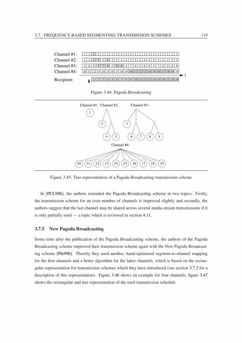
3.7. FREQUENCY-BASED SEGMENTING TRANSMISSION SCHEMES 119
Channel #3:Channel #2:Channel #1:
Recipient:
Channel #4: 10 11 12 13
111 1 1 1 1 1 11 1 1 1 1 1 1 11
1514 11 1312 1514
2 4 52 2 4 52 2 4 52 2 4 52 2 4 5
8 3 97 3 6 8 3 97 3 6 3 97 3 63 6
1716 18 19 1716 18 19
761 2 3 54 15148 9 1110 1312 1716 18 19
11
2 2
8 8
10 10t
1
Figure 3.44: Pagoda Broadcasting
19
1
4 5
Channel #3:Channel #2:Channel #1:
3
6 7 8 9
Channel #4:
11 12 13 14 15 16 17 1810
2
Figure 3.45: Tree representation of a Pagoda Broadcasting transmission scheme
In [PCL99b], the authors extended the Pagoda Broadcasting scheme in two topics: Firstly,
the transmission scheme for an even number of channels is improved slightly and secondly, the
authors suggest that the last channel may be shared across several media stream transmissions if it
is only partially used — a topic which is reviewed in section 4.11.
3.7.5 New Pagoda Broadcasting
Some time after the publication of the Pagoda Broadcasting scheme, the authors of the Pagoda
Broadcasting scheme improved their transmission scheme again with the New Pagoda Broadcast-
ing scheme [Pâr99b]. Thereby they used another, hand-optimized segment-to-channel mapping
for the first channels and a better algorithm for the latter channels, which is based on the rectan-
gular representation for transmission schemes which they have introduced (see section 3.7.2 for a
description of this representation). Figure 3.46 shows an example for four channels, figure 3.47
shows the rectangular and tree representation of the used transmission schedule.

120 CHAPTER 3. MEDIA TRANSMISSION SCHEMES
Technical classification Functional classification
Communication type:
One-to-manyBack-channel:
Not requiredMedia-on-demand topology:
StarSender bandwidth:
Multiple of media stream bit rateSender storage seeks:
Single position per slotReceiver bandwidth:
Multiple of media stream bit rateReceiver storage size:
Partial media stream bufferingReceiver storage seeks:
Single position per slot
Media scheduling:
Pro-active media-on-demandPlayback control:
No playback controlContent navigation:
No non-continuous navigationDynamic schedule changes:
No dynamic scheduling change supportDynamic content changes:
No dynamic content supportVariable-bit-rate media support:
No dynamic content supportLive streaming capability:
Not live streaming capable
Table 3.38: Classification for Pagoda Broadcasting transmissions
Channel #3:Channel #2:Channel #1:
Channel #4:
Recipient: 19
5 10 15 18
761 2 3 54
111 1 1 1 1 1 11 1 1 1 1 1 1 11 1
521 105t
2017 523
15148 9 1110 1312
2 4 82 2 4 92 2 4 82 2 4 92 2 4 82
12 3 137 3 6 14 3 257 3 6 12 3 137 3 63 6
1611 19 22 1511 18 24
1716 18
1
Figure 3.46: New Pagoda Broadcasting
Technical classification Functional classification
Communication type:
One-to-manyBack-channel:
Not requiredMedia-on-demand topology:
StarSender bandwidth:
Multiple of media stream bit rateSender storage seeks:
Single position per slotReceiver bandwidth:
Multiple of media stream bit rateReceiver storage size:
Partial media stream bufferingReceiver storage seeks:
Single position per slot
Media scheduling:
Pro-active media-on-demandPlayback control:
No playback controlContent navigation:
No non-continuous navigationDynamic schedule changes:
No dynamic scheduling change supportDynamic content changes:
No dynamic content supportVariable-bit-rate media support:
No dynamic content supportLive streaming capability:
Not live streaming capable
Table 3.39: Classification for New Pagoda Broadcasting transmissions
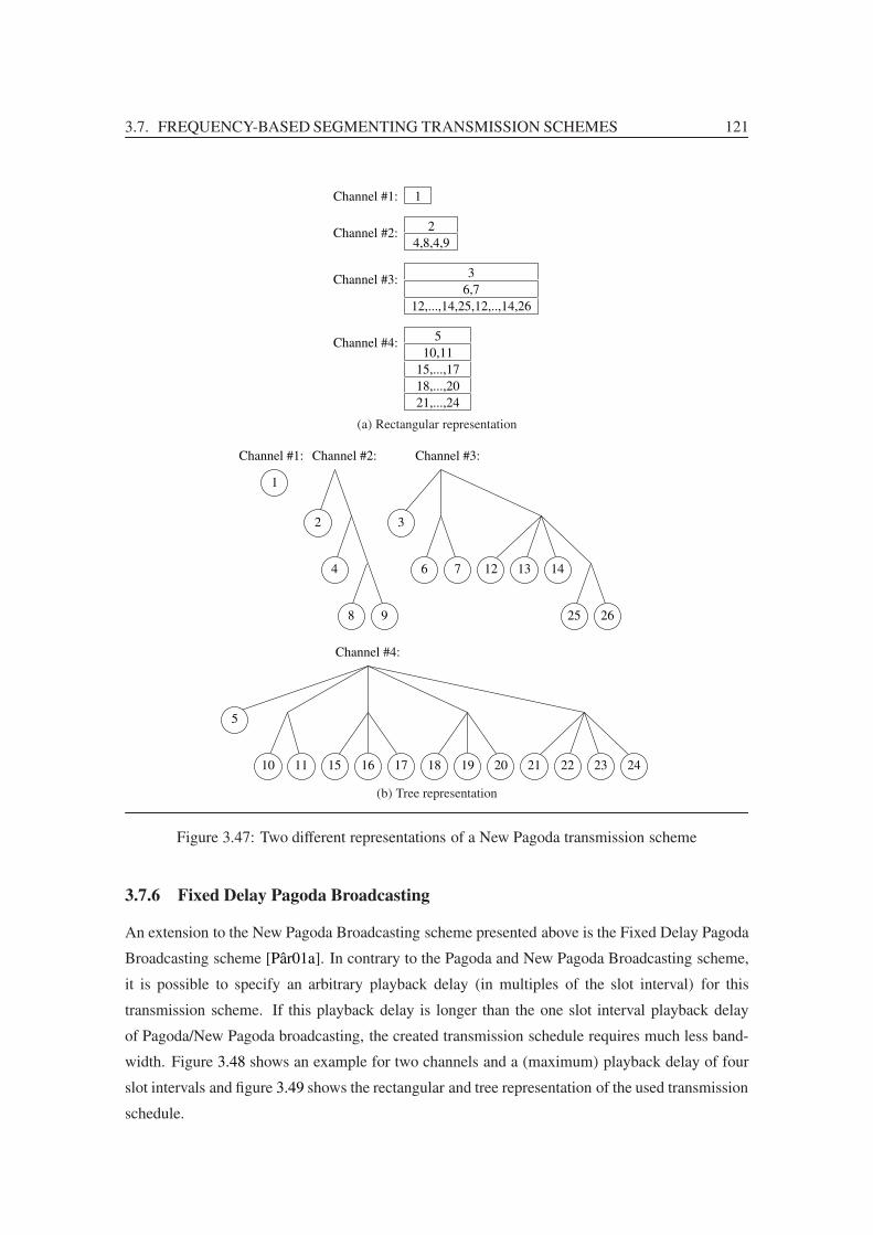
3.7. FREQUENCY-BASED SEGMENTING TRANSMISSION SCHEMES 121
Channel #2:
Channel #3:
Channel #1: 1
Channel #4: 5
4,8,4,92
10,11
18,...,2015,...,17
21,...,24
6,73
12,...,14,25,12,..,14,26
(a) Rectangular representation
Channel #3:
2
1
4
Channel #1:
6 7
8 9
12 13 14
25 26
3
10 11 15 16 17 18 19 20 21 22 23 24
Channel #4:
Channel #2:
5
(b) Tree representation
Figure 3.47: Two different representations of a New Pagoda transmission scheme
3.7.6 Fixed Delay Pagoda Broadcasting
An extension to the New Pagoda Broadcasting scheme presented above is the Fixed Delay Pagoda
Broadcasting scheme [Pâr01a]. In contrary to the Pagoda and New Pagoda Broadcasting scheme,
it is possible to specify an arbitrary playback delay (in multiples of the slot interval) for this
transmission scheme. If this playback delay is longer than the one slot interval playback delay
of Pagoda/New Pagoda broadcasting, the created transmission schedule requires much less band-
width. Figure 3.48 shows an example for two channels and a (maximum) playback delay of four
slot intervals and figure 3.49 shows the rectangular and tree representation of the used transmission
schedule.

122 CHAPTER 3. MEDIA TRANSMISSION SCHEMES
Additionally, the Fixed Delay Pagoda Broadcasting scheme allows defining a limit for the
receiver bandwidth to create a transmission schedule which does not exceed this limit.
In sections 4.4 and 4.5, the effects of the playback delay and decoupling the playback delay
from the slot interval are examined in detail, in section 4.18 the consequences of a limited receiver
bandwidth is studied again.
Channel #1:
Recipient:
Channel #2:
1 24 5
6 9 713 10 14 118 15 6 1612 7 9 817 10 13 86
1 3 2 4 1 5 2 3 1 3 2 4 1 5 2 3
7654 15148 9 1110 1312 1631 2
t
Figure 3.48: Fixed Delay Pagoda Broadcasting
6,...,89,...,1213,...,17
1,23,...,5
Channel #2:
Channel #1:
(a) Rectangular representation
Channel #1:
7 8 9 10 11 12 13 14 15 16 17
Channel #2:
1 2 3 4 5
6
(b) Tree representation
Figure 3.49: Two different representations of a Fixed Delay Pagoda transmission scheme
3.7.7 Variable Bandwidth Broadcasting
The Variable Bandwidth Broadcasting scheme [PL03] is an enhanced version of the New Pagoda
Broadcasting scheme: It uses a similar layout and reaches an efficiency similar to the Fixed Delay

3.7. FREQUENCY-BASED SEGMENTING TRANSMISSION SCHEMES 123
Technical classification Functional classification
Communication type:
One-to-manyBack-channel:
Not requiredMedia-on-demand topology:
StarSender bandwidth:
Multiple of media stream bit rateSender storage seeks:
Single position per slotReceiver bandwidth:
! Configurable multiple of media stream bit rateReceiver storage size:
Partial media stream bufferingReceiver storage seeks:
Single position per slot
Media scheduling:
Pro-active media-on-demandPlayback control:
No playback controlContent navigation:
No non-continuous navigationDynamic schedule changes:
No dynamic scheduling change supportDynamic content changes:
No dynamic content supportVariable-bit-rate media support:
No dynamic content supportLive streaming capability:
Not live streaming capable
Table 3.40: Classification for Fixed-Delay Pagoda Broadcasting transmissions
Pagoda Broadcasting scheme with W + = δ. Figure 3.50 shows an example of a Variable Band-
width Broadcasting transmission.
Channel #2:Channel #1:
Channel #3:
Recipient: 2 3 5 97
1 11 11 111 11 11
252 2524 524
3 3 97 3 6 38 97
4
4
6
6
8
8
2
t1
Figure 3.50: Variable Bandwidth Broadcasting
The most interesting point about the Variable Bandwidth Broadcasting scheme is that it sup-
ports dynamic bandwidth changes, similar to the Seamless Staircase Broadcasting scheme and the
Seamless Fast Broadcasting scheme.
The authors of the Variable Bandwidth Broadcasting scheme also analyzed one of the condi-
tions which is necessary for supporting dynamic bandwidth changes: When a channel is added
and the playback delay is decreased from one to a half slot interval, all segments which had been
scheduled with their maximum required period are sent too infrequently in the new transmission
scheme. The Variable Bandwidth Broadcasting scheme solves this problem by moving these seg-
ments to new positions (typically by moving all these segments in a chain by one position, i. e. by
moving the first segment to the new channel, the second to the old position of the first segment and
so on). The authors also proposed the idea to artificially decrease the period by one for the latter
segments to prevent that too much segments have to be moved and the transition takes too long.
Unfortunately, the authors missed to recognize a second condition: When a segment is moved

124 CHAPTER 3. MEDIA TRANSMISSION SCHEMES
forward in time, it is possible that this interrupts ongoing playbacks. Figure 3.51 shows an example
where this segment moving causes a hole in a playback. This approach (together with a solution
for the moving problem) is revised in section 4.15.
Recipient:
5
BA7 7B3 B6 BA− 8 8B6−
1 2 5 A B6 6
A4
B4
B4A4 BA8 8
BA9 9BA8 8
9
97
73
1 11 11 A BA
A
BA
A A
BA BA
AA A A A A
2
1 1 1 1 1
2 21 1 1 12 2
1 11 1A1
B1
t
A
BA
A1
2 1
1 A
BA
A1
2 1
1
25242
338
A A3 3A6 B2 BA5 5 B2 A3A6 B4 B2 BA5
Figure 3.51: Ongoing transmissions may be interrupted when a channel is added using the VariableBandwidth Broadcasting scheme
Technical classification Functional classification
Communication type:
One-to-manyBack-channel:
Not requiredMedia-on-demand topology:
StarSender bandwidth:
Multiple of media stream bit rateSender storage seeks:
Single position per slotReceiver bandwidth:
Multiple of media stream bit rateReceiver storage size:
Partial media stream bufferingReceiver storage seeks:
Single position per slot
Media scheduling:
Pro-active media-on-demandPlayback control:
No playback controlContent navigation:
No non-continuous navigationDynamic schedule changes:
! Full dynamic scheduling change supportDynamic content changes:
No dynamic content supportVariable-bit-rate media support:
No dynamic content supportLive streaming capability:
Not live streaming capable
Comment:
!!! Dynamic scheduling change support is malfunctioning
Table 3.41: Classification for Variable Bandwidth Broadcasting transmissions
3.7.8 Greedy Broadcasting/Recursive Frequency Splitting
The next transmission scheme has been developed independently by two groups at nearly the
same time as Greedy Broadcasting scheme [BNL02, BNL03, CST00] and Recursive Frequency
Splitting scheme [TYC02].
While the Recursive Frequency Splitting scheme uses a more mathematical description of the
algorithm, the authors of the Greedy Broadcasting scheme introduced the tree-based representation
for transmission schemes and developed a graph-based algorithm for generating the tree. This

3.7. FREQUENCY-BASED SEGMENTING TRANSMISSION SCHEMES 125
algorithm inserts the segments one-by-one as nodes into the transmission trees at a position which
is selected by a simple heuristic:
1. Primarily, the segment is inserted in such a way that the segment is transmitted as often as
necessary but as infrequently as possible, so it satisfies the condition for correct playback
but wastes the least bandwidth.
2. If the bandwidth loss for several nodes is equal, the node with the highest transmission
period is selected, leaving the nodes with low periods for the remaining segments.
3. If this node has a transmission period low enough to carry more than the segment to be
inserted, it is split into several parts of equal period, leaving the remaining nodes for other
segments. In the tree representation, these splits are represented by non-leaf nodes, while
the inserted segments are the leaf-nodes.
Figure 3.52 shows an example for four channels and figure 3.53 shows the tree representation of the
used transmission schedule. This transmission scheme will be reviewed extensively in chapter 4
as its full potential has not been tapped yet.
Channel #3:Channel #2:Channel #1:
Channel #4:
Recipient: 19
5 10 12 14
761 2 3 54
111 1 1 1 1 1 11 1 1 1 1 1 1 11 1
515 105t
1412 525
15148 9 1110 1312
2 4 82 2 4 162 2 4 82 2 4 172 2 4 82
9 3 187 3 6 22 3 97 3 6 19 3 237 3 63 6
1311 20 24 1311 21 15
1716 18
1
Figure 3.52: Greedy Broadcasting/Recursive Frequency Splitting
3.7.9 Fuzzycast
Fuzzycast [JWX02] is based on the Harmonic Equal-Bandwidth Broadcasting scheme, but re-
moves its high bandwidth requirements using a heuristic algorithm: When it encounters a slot
interval which contains too many segments, it decides to move the highest segment(s) to another
slot interval, either forward or backward in time. Unfortunately, moving segments has a draw-
back: If segments are transmitted earlier this way, the bandwidth is increased and the transmission
scheme looses some efficiency. If segments are transmitted later, the playback delay has to be
increased, which lowers the efficiency, too.
A major disadvantage of the Fuzzycast transmission scheme is that its bandwidth requirement
or playback delay cannot be guaranteed for a permanent transmission: As the moving process
is heuristic, there is no way to predict how much free slots are available in the neighborhood of
a specific segment position (assuming that the granted bandwidth is not so high that nearly no

126 CHAPTER 3. MEDIA TRANSMISSION SCHEMES
21
1
4
Channel #1:
6 7
8
9
22 23
3
Channel #2: Channel #3:
16 17
18 19
10 11 12 13 14 15 24 25
Channel #4:
5
20
2
Figure 3.53: Tree representation of a Greedy Broadcasting/Recursive Frequency Splitting trans-mission scheme
Technical classification Functional classification
Communication type:
One-to-manyBack-channel:
Not requiredMedia-on-demand topology:
StarSender bandwidth:
Multiple of media stream bit rateSender storage seeks:
Single position per slotReceiver bandwidth:
Multiple of media stream bit rateReceiver storage size:
Partial media stream bufferingReceiver storage seeks:
Single position per slot
Media scheduling:
Pro-active media-on-demandPlayback control:
No playback controlContent navigation:
No non-continuous navigationDynamic schedule changes:
No dynamic scheduling change supportDynamic content changes:
No dynamic content supportVariable-bit-rate media support:
No dynamic content supportLive streaming capability:
Not live streaming capable
Table 3.42: Classification for Greedy Broadcasting/Recursive Frequency Splitting transmissions
moving is required). As a consequence, the Fuzzycast scheme has an unpredictable bandwidth
consumption or playback delay because the bandwidth can only be examined if the playback is

3.7. FREQUENCY-BASED SEGMENTING TRANSMISSION SCHEMES 127
simulated until end. Nevertheless, the idea of moving segments is revised later in section 4.13 in
the context of efficient terminations of ongoing transmissions.
One interesting improvement to reduce the number of segment moves has been mentioned by
the authors of the Fuzzycast Broadcasting scheme: If several transmissions are grouped together,
the probability to find a free slot at the destined position or in its near neighborhood is much higher
than for a single transmission. Therefore, the sender bandwidth can be reduced by this grouping
for each of the transmissions. The not mentioned drawback of this grouping is that the receiver
bandwidth must be higher when one transmission uses free slots of another one. This idea is
resumed in section 4.11.
Technical classification Functional classification
Communication type:
One-to-manyBack-channel:
Not requiredMedia-on-demand topology:
StarSender bandwidth:
Multiple of media stream bit rateSender storage seeks:
Single position per slotReceiver bandwidth:
Multiple of media stream bit rateReceiver storage size:
Partial media stream bufferingReceiver storage seeks:
Single position per slot
Media scheduling:
Pro-active media-on-demandPlayback control:
No playback controlContent navigation:
No non-continuous navigationDynamic schedule changes:
No dynamic scheduling change supportDynamic content changes:
No dynamic content supportVariable-bit-rate media support:
No dynamic content supportLive streaming capability:
Not live streaming capable
Table 3.43: Classification for Fuzzycast Broadcasting transmissions
3.7.10 Dual Broadcasting
The Dual Broadcasting scheme [PCL99a] is a transmission scheme which supports receiver sys-
tems without and with local storage. To support both systems at the same time, a transmission
scheme which requires no storage (e. g. Round-Robin transmissions or Staggered Broadcasting)
and one which uses storage at the recipient systems (e. g. Fast Broadcasting or Pagoda Broadcast-
ing) have to be used at the same time.
But a simple combination of these two transmission schemes is a waste of bandwidth as the
recipient systems which are equipped with storage could benefit from the no-storage transmissions.
The authors of the Dual Broadcasting scheme therefore developed a transmission scheme where
the storage-based transmission relies on the no-storage transmission.
Figure 3.54 shows an example for a Dual Broadcasting transmission. Recipient #1 in this

128 CHAPTER 3. MEDIA TRANSMISSION SCHEMES
example does not need any storage whild recipient #2 joined the transmission at a time where
storage is required.
Recipient #1:
Channel #4:Channel #3:Channel #2:
Recipient #2:
Channel #1:
t
16 1712 1310 1198 14 154 5321 6 7
1 2 3 4
10 5 11 12
5 6 7 8 9 1110 12 13 14 15 16 17 21 3
313 34 5 84
2 1 11 1 1 11 1 1 11 1 1 11 1 2 11
7 2 214 8 2 16 2 26 7 2 3 2 36 4 73 4
415 3 5 109 5 11−
761 2 3 54 15148 9 1110 1312 1716
4 5 6 7 8 9 10
1 1 1 1 1 1 1
2 14 2 8 2 216
3 312 13 15 4 5
Figure 3.54: Dual Broadcasting
Unfortunately, the Dual Broadcasting scheme is not a pure frequency-based transmission
scheme as it transmits the segments at non-constant frequency. As a consequence, transmission
schemes according to this scheme cannot be created as simple as the other proposed schemes.
Even the authors of the Dual Broadcasting scheme only presented two schedules for this scheme
(one for three and one for four channels) without providing an algorithm for general construction.
Another thing to note here is that the Fast Broadcasting scheme (see section 3.7.2) already sup-
ports a reception without storage with a maximum playback delay of one media stream duration,
but the Dual Broadcasting scheme outperforms this.
Technical classification Functional classification
Communication type:
One-to-manyBack-channel:
Not requiredMedia-on-demand topology:
StarSender bandwidth:
Multiple of media stream bit rateSender storage seeks:
Single position per slotReceiver bandwidth:
Multiple of media stream bit rateReceiver storage size:
! None or partial media stream bufferingReceiver storage seeks:
! None or single position per slot
Media scheduling:
Pro-active media-on-demandPlayback control:
No playback controlContent navigation:
No non-continuous navigationDynamic schedule changes:
No dynamic scheduling change supportDynamic content changes:
No dynamic content supportVariable-bit-rate media support:
No dynamic content supportLive streaming capability:
Not live streaming capable
Comment:
! Different service for receiver systems with and without storage
Table 3.44: Classification for Dual Broadcasting transmissions

3.7. FREQUENCY-BASED SEGMENTING TRANSMISSION SCHEMES 129
3.7.11 Comparison of Frequency-Based Segmenting Transmission Schemes
Comparing the frequency-based segmenting transmission schemes with each other is a much sim-
pler task than comparing size-based or bandwidth-based schemes as the differences between the
various frequency-based schemes are much less significant. Besides of the layout of the segments
on the channels, the transmission schemes differ in the following points:
• For the Fixed Delay Pagoda Broadcasting scheme and the Harmonic Equal-Bandwidth
Broadcasting scheme, the playback delay can be defined independent of the segment size.
• The Fixed Delay Pagoda Broadcasting scheme supports receiver systems with limited re-
ceiver bandwidth or storage size.
• The Fast Broadcasting scheme and the Dual Broadcasting scheme support receiver systems
without storage.
• The Seamless Fast Broadcasting scheme and the Variable Bandwidth Broadcasting scheme
support seamless bandwidth changes for ongoing transmissions.
Similar to the comparison charts for size- and bandwidth-based transmission schemes, it is as-
sumed that the receiver systems provide an unlimited amount of bandwidth and storage to receive
the transmission. Additionally, the ability to change the playback delay dynamically is ignored
here.
Figure 3.55 shows the efficiency of the frequency-based transmission schemes if the slot
duration equals the playback delay. As expected, the (practically unusable) Harmonic Equal-
Bandwidth Broadcasting scheme provides the highest efficiency of all these transmission schemes,
nearby followed by the Greedy Broadcasting/Recursive Frequency Splitting scheme. But the Har-
monic Equal-Bandwidth Broadcasting scheme is still far away from the theoretical lower bound
(i. e. from an efficiency η = 1) if the segment size is bound to the playback delay, esp. for long
playback delays.
If the transmission scheme supports to select the playback delay independent from the segment
size, the segment size can be decreased while keeping the playback delay constant. Figure 3.56
shows the result of this procedure for the two transmission schemes which support this functional-
ity. In this case, both transmission schemes operate much better, the Harmonic Equal-Bandwidth
Broadcasting scheme even operates at 100 %.
The Dual Broadcasting scheme has been omitted from these comparisons as no algorithm for
generation of large Dual Broadcasting transmission schedules is available.

130 CHAPTER 3. MEDIA TRANSMISSION SCHEMES
10%
20%
30%
40%
50%
60%
70%
80%
90%
100%
0.0002 0.0005 0.001 0.002 0.005 0.01 0.02 0.05 0.1 0.2
Ban
dwid
th e
ffic
ienc
y
Playback delay as fraction of media stream duration
Harmonic Equal Bandwidth Broadcasting (W+=δ)Greedy Broadcasting/Recursive Frequency Splitting
New Pagoda BroadcastingVariable Bandwidth Broadcasting
Fixed Delay Pagoda Broadcasting (W+=δ)Pagoda Broadcasting
Fast BroadcastingSeamless Fast Broadcasting
Figure 3.55: Efficiency of frequency-based schemes if the playback delay equals the slot interval
10%
20%
30%
40%
50%
60%
70%
80%
90%
100%
0.0002 0.0005 0.001 0.002 0.005 0.01 0.02 0.05 0.1 0.2
Ban
dwid
th e
ffic
ienc
y
Playback delay as fraction of media stream duration
Harmonic Equal Bandwidth Broadcasting (δ=d/7200)Fixed Delay Pagoda Broadcasting (δ=d/7200)
Figure 3.56: Efficiency of frequency-based schemes for which the slot interval can be decreasedindependent of the playback delay

3.8. REACTIVE-PRO-ACTIVE-HYBRID TRANSMISSION SCHEMES 131
3.8 Reactive-Pro-Active-Hybrid Transmission Schemes
The above presented transmission schemes are either reactive or pro-active by design. In this
section, reactive-pro-active-hybrid transmission schemes are presented which use combinations
of reactive and pro-active design patterns.
One way to combine reactive and pro-active transmission schemes is to send part of the media
stream using a reactive transmission scheme and the remainder using a pro-active scheme. The
reason for combining a reactive and a pro-active transmission scheme this way is that the most
bandwidth of a media transmission is required for the transmission of the first segments which are
received only by a few recipients, thus the most bandwidth is wasted by the transmission of the
first part of the media stream if only few recipients are listening to the transmission. If a reactive
transmission scheme is used for the first part of the media stream, this bandwidth can be saved,
providing at the same time a short playback delay (or even immediate access, depending only on
the reactive scheme).
Another way to apply reactive behavior to a pro-active transmission scheme is to use playback
request to evaluate which segment transmissions are not needed by any recipient and omitting the
transmission of these segments in a pro-active transmission schedule.
3.8.1 Unified Video-on-Demand Broadcasting
The Unified Video-on-Demand Broadcasting scheme [Lee99] is a combination of the Staggered
Broadcasting scheme (see section 3.4.2 with Point-to-Point transmissions (see section 3.3.1: As
the playback delay of the Staggered Broadcasting scheme is very high, the Unified Video-on-
Demand Broadcasting scheme uses Point-to-Point transmissions to transmit the beginning of the
media stream to recipients which called in at an ongoing transmission. That way, the Unified
Video-on-Demand Broadcasting scheme provides immediate access without the need to transmit
the whole media stream to the recipients.
3.8.2 Batching Unified Video-on-Demand Broadcasting
Similar to the Unified Video-on-Demand Broadcasting scheme of the last subsection, the Batching
Unified Video-on-Demand Broadcasting scheme [LL00] benefits from the Staggered Broadcast-
ing scheme. But instead of using Point-to-Point transmissions for the beginning of the media
streams, this scheme broadcasts the beginning at times determined by a Batching scheme (see
section 3.3.2). Consequently, the Batching Unified Video-on-Demand Broadcasting scheme does
not offer immediate access any more but still reduces the playback delay of the Staggered Broad-
casting scheme.

132 CHAPTER 3. MEDIA TRANSMISSION SCHEMES
Technical classification Functional classification
Communication type:
One-to-manyBack-channel:
RequiredMedia-on-demand topology:
StarSender bandwidth:
Multiple of media stream bit rateSender storage seeks:
Single position per channelReceiver bandwidth:
! Twice the media stream bit rateReceiver storage size:
Partial media stream bufferingReceiver storage seeks:
Single position per channel
Media scheduling:
! Combined reactive/pro-active media-on-demandPlayback control:
! Fixed jump playback controlContent navigation:
No non-continuous navigationDynamic schedule changes:
No dynamic scheduling change supportDynamic content changes:
No dynamic content supportVariable-bit-rate media support:
No dynamic content supportLive streaming capability:
! Live streaming capable
Table 3.45: Classification for Unified Video-on-Demand Broadcasting transmissions
Technical classification Functional classification
Communication type:
One-to-manyBack-channel:
RequiredMedia-on-demand topology:
StarSender bandwidth:
Multiple of media stream bit rateSender storage seeks:
Single position per channelReceiver bandwidth:
Twice the media stream bit rateReceiver storage size:
Partial media stream bufferingReceiver storage seeks:
Single position per channel
Media scheduling:
! Combined reactive/pro-active media-on-demandPlayback control:
! Fixed jump playback controlContent navigation:
No non-continuous navigationDynamic schedule changes:
No dynamic scheduling change supportDynamic content changes:
No dynamic content supportVariable-bit-rate media support:
No dynamic content supportLive streaming capability:
! Live streaming capable
Table 3.46: Classification for Batching Unified Video-on-Demand Broadcasting transmissions
3.8.3 Reactive Broadcasting
Similar to the above two transmission schemes, the Reactive Broadcasting scheme [PCL00a] is
actually a combination of two transmission schemes: A reactive transmission is used for the trans-
mission of the first segment of the media stream and a pro-active transmission scheme is used
for the remaining segments. But instead of using Staggered Broadcasting combined with Point-
to-Point Transmissions or Batching, the authors of [PCL00a] suggested to use Tapping (see sec-
tion 3.3.5) as reactive scheme and a Pagoda-like scheme (see section 3.7.4) as pro-active scheme.

3.8. REACTIVE-PRO-ACTIVE-HYBRID TRANSMISSION SCHEMES 133
Technical classification Functional classification
Communication type:
One-to-manyBack-channel:
RequiredMedia-on-demand topology:
StarSender bandwidth:
Multiple of media stream bit rateSender storage seeks:
Single position per slotReceiver bandwidth:
Multiple of media stream bit rateReceiver storage size:
Partial media stream bufferingReceiver storage seeks:
Single position per slot
Media scheduling:
! Combined reactive/pro-active media-on-demandPlayback control:
No playback controlContent navigation:
No non-continuous navigationDynamic schedule changes:
No dynamic scheduling change supportDynamic content changes:
No dynamic content supportVariable-bit-rate media support:
No dynamic content supportLive streaming capability:
Not live streaming capable
Table 3.47: Classification for Reactive Broadcasting transmissions
3.8.4 Dynamic Skyscraper Broadcasting
The Dynamic Skyscraper Broadcasting scheme [EV98] makes two modifications to the Skyscraper
Broadcasting scheme presented in section 3.5.3. Firstly, it divides subsequent segment transmis-
sions up to a specific length to transmission clusters and allows that transmission clusters can
be dropped if no recipient is listening to the appropriate transmission. As they suggest using the
same transmission cluster sizes for all media streams, this spare bandwidth can simply be reused
for other media stream transmissions. Figure 3.57 illustrates the use of transmission clusters.
Secondly, they proposed three new broadcasting series:
A : 1,2,2,4,4,8,8,16,16,32,32,64,64,128,128, . . .
B : 1,2,2,6,6,12,12,24,24,48,48,96,96,192,192, . . .
C : 1,2,2,6,6,12,12,36,36,72,72,216,216,432,432, . . .
(3.38)
These broadcasting series avoid conflicts and holes in transmission clusters which would occur if
the original broadcasting series are used. Broadcasting series B and C additionally require that the
receiver system is able to receive three channels at a time, while for sequence A two channels still
suffice.
3.8.5 Partitioned Dynamic Skyscraper Broadcasting
The Partitioned Dynamic Skyscraper Broadcasting scheme [EFV99] is a variant of the Dynamic
Skyscraper Broadcasting scheme presented above. Instead of using a single sender, the Partitioned
Dynamic Skyscraper Broadcasting scheme assumes a hierarchical setup, consisting of a global

134 CHAPTER 3. MEDIA TRANSMISSION SCHEMES
6
1 1 1 1 1 1 1 1Channel #1:
Channel #2:
Channel #3:
Channel #4:
Channel #5:
Channel #6:
TransmissionCluster Size
Recipient:
5 5
6
4 4
3 3 3 3
2 2 2 2
1 2 3 4 5t
Figure 3.57: Dynamic Skyscraper Broadcasting
Technical classification Functional classification
Communication type:
One-to-manyBack-channel:
RequiredMedia-on-demand topology:
StarSender bandwidth:
Multiple of media stream bit rateSender storage seeks:
Single position per slotReceiver bandwidth:
! Twice or three times the media stream bit rateReceiver storage size:
Partial media stream bufferingReceiver storage seeks:
Single position per slot
Media scheduling:
! Combined reactive/pro-active media-on-demandPlayback control:
No playback controlContent navigation:
No non-continuous navigationDynamic schedule changes:
No dynamic scheduling change supportDynamic content changes:
No dynamic content supportVariable-bit-rate media support:
No dynamic content supportLive streaming capability:
Not live streaming capable
Table 3.48: Classification for Dynamic Skyscraper Broadcasting transmissions
sender system and a set of regional sender systems. Therefore, the Partitioned Dynamic Skyscraper
Broadcasting scheme requires that the receiver systems are able to receive data simultaneously
from the global sender system and from its next regional sender system (doubling the bandwidth
requirement for the clients and assuming a network which benefits from regional sender systems).
The Partitioned Dynamic Skyscraper Broadcasting scheme uses this setup by transmitting the
first segments of a media stream using regional sender systems and sending the latter segments
from the global sender system. This reduces the global network utilization as the most bandwidth
is required for the first segments which are only transmitted regionally. Figure 3.58 shows an
example for a Partitioned Dynamic Skyscraper Broadcasting transmission.

3.8. REACTIVE-PRO-ACTIVE-HYBRID TRANSMISSION SCHEMES 135
2 4 5
t
1 1Regional channel #1:
Regional channel #2:
Regional channel #3:
1 1
2 2
3 3
Regional TransmissionCluster Size
Remote TransmissionCluster Size
Remote channel #1:
Remote channel #2:
4
5
4
Recipient: 1 3
Figure 3.58: Partitioned Dynamic Skyscraper Broadcasting
Technical classification Functional classification
Communication type:
One-to-manyBack-channel:
RequiredMedia-on-demand topology:
StarSender bandwidth:
Multiple of media stream bit rateSender storage seeks:
Single position per slotReceiver bandwidth:
! Four to six times the media stream bit rateReceiver storage size:
Partial media stream bufferingReceiver storage seeks:
Single position per slot
Media scheduling:
! Combined reactive/pro-active media-on-demandPlayback control:
No playback controlContent navigation:
No non-continuous navigationDynamic schedule changes:
No dynamic scheduling change supportDynamic content changes:
No dynamic content supportVariable-bit-rate media support:
No dynamic content supportLive streaming capability:
Not live streaming capable
Table 3.49: Classification for Partitioned Dynamic Skyscraper Broadcasting transmissions
3.8.6 Universal Broadcasting
The Universal Broadcasting scheme [PCL00b] is based on the Fast Broadcasting scheme (see
section 3.7.2), but it uses two modifications to save bandwidth if only few recipients are requesting
the media:
1. Only required segments are sent at the latest possible time. To ascertain which segments are
required, this transmission scheme is based on requests from recipient systems to determine
at which slot intervals recipients have started a playback.

136 CHAPTER 3. MEDIA TRANSMISSION SCHEMES
2. The segments of each channel may be shifted if no ongoing playback is interfered thereby.
Figure 3.59 shows an example for a Universal Broadcasting transmission with two recipients.
Recipient #1:
Channel #1:
Channel #4:Channel #3:Channel #2:
Recipient #2: 12
32
761 2 3 54
1 2 3 54
654
1
32
54
8 9 1110t
1312 1514
1514
76
76
8 9 1110 1312
8 9 1110 13
1
Figure 3.59: Universal Broadcasting
Using these two modifications, the Universal Broadcasting scheme needs no bandwidth if no
playbacks are active and it only needs one transmission channel if only one request is active.
As the authors have examined, the Universal Broadcasting scheme needs less bandwidth than
the (pro-active) New Pagoda transmission scheme for up to 55 requests per hour if a two hour
media stream is transmitted in 127 segments. For higher request rates, the Universal Broadcasting
scheme converges to the Fast Broadcasting scheme.
Another thing to note here is that it is possible to apply the first of the aforementioned mod-
ifications — suppression of segment transmissions which are not needed by any receiver system
— to any segmenting transmission scheme. The second modification — shifting of segments in
channels — can only by applied to transmission schemes which transmit all segments of a chan-
nel with the same frequency, thus it can only be applied to the Fast Broadcasting scheme of the
presented frequency-based group of transmission schemes. (By theory, it would also be possible
to apply it to transmission schemes of e. g. the size-based group as they only transmit a single
segment per channel, but as their efficiency is below that of Fast Broadcasting this is not studied
here in more detail.)
In section 4.12, the idea behind this approach is reviewed in a generalized version.
3.8.7 Channel-Based Heuristic Distribution
The Channel-based Heuristic Distribution scheme [ZP02] is the result of a further development
of the Universal Broadcasting scheme. It produces similar results as the Universal Broadcasting
scheme, but it has been extended to support increased playback delays. Figure 3.60 shows an
example for this transmission scheme with a playback delay of two slot intervals.
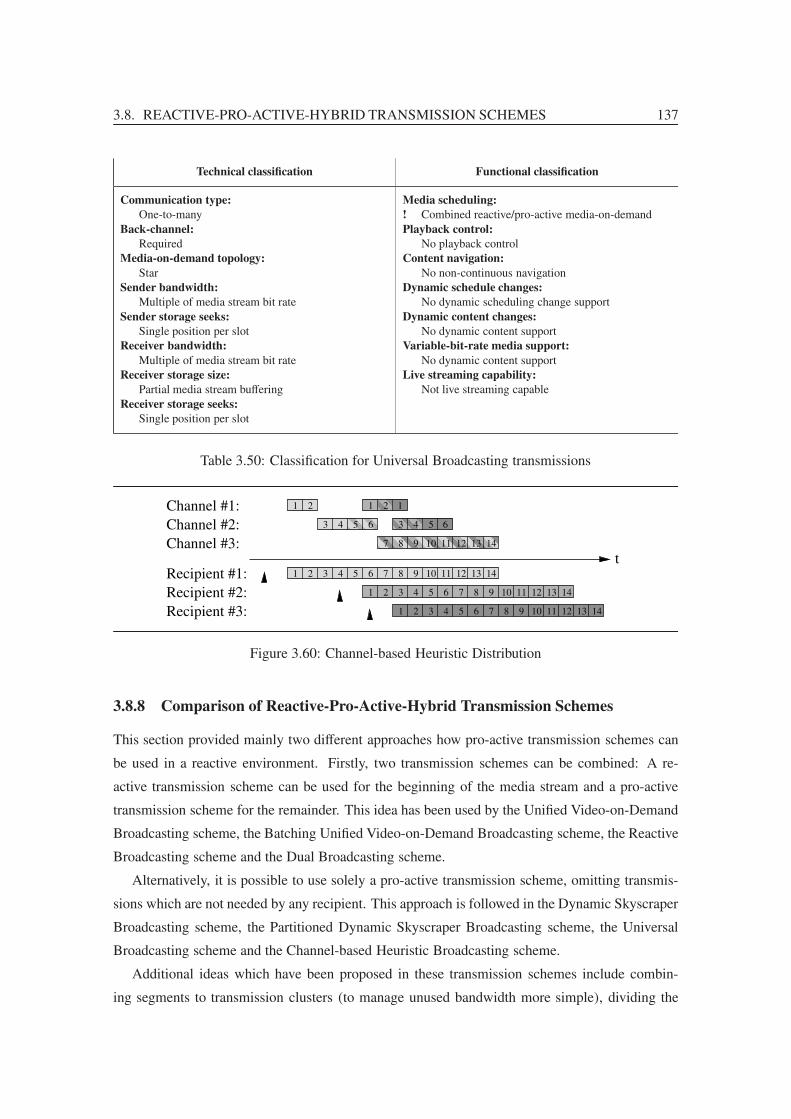
3.8. REACTIVE-PRO-ACTIVE-HYBRID TRANSMISSION SCHEMES 137
Technical classification Functional classification
Communication type:
One-to-manyBack-channel:
RequiredMedia-on-demand topology:
StarSender bandwidth:
Multiple of media stream bit rateSender storage seeks:
Single position per slotReceiver bandwidth:
Multiple of media stream bit rateReceiver storage size:
Partial media stream bufferingReceiver storage seeks:
Single position per slot
Media scheduling:
! Combined reactive/pro-active media-on-demandPlayback control:
No playback controlContent navigation:
No non-continuous navigationDynamic schedule changes:
No dynamic scheduling change supportDynamic content changes:
No dynamic content supportVariable-bit-rate media support:
No dynamic content supportLive streaming capability:
Not live streaming capable
Table 3.50: Classification for Universal Broadcasting transmissions
Recipient #1:
Channel #1:Channel #2:Channel #3:
Recipient #3:Recipient #2:
t761 2 3 54 8 9 1110 1312 14
1 2 3 54 76 8 9 1110 1312 14
1 2
1 2 3 54 76 8 9 1110 1312 14
1 2 1
7 148 9 1110 1312
3 54 6 3 54 6
Figure 3.60: Channel-based Heuristic Distribution
3.8.8 Comparison of Reactive-Pro-Active-Hybrid Transmission Schemes
This section provided mainly two different approaches how pro-active transmission schemes can
be used in a reactive environment. Firstly, two transmission schemes can be combined: A re-
active transmission scheme can be used for the beginning of the media stream and a pro-active
transmission scheme for the remainder. This idea has been used by the Unified Video-on-Demand
Broadcasting scheme, the Batching Unified Video-on-Demand Broadcasting scheme, the Reactive
Broadcasting scheme and the Dual Broadcasting scheme.
Alternatively, it is possible to use solely a pro-active transmission scheme, omitting transmis-
sions which are not needed by any recipient. This approach is followed in the Dynamic Skyscraper
Broadcasting scheme, the Partitioned Dynamic Skyscraper Broadcasting scheme, the Universal
Broadcasting scheme and the Channel-based Heuristic Broadcasting scheme.
Additional ideas which have been proposed in these transmission schemes include combin-
ing segments to transmission clusters (to manage unused bandwidth more simple), dividing the

138 CHAPTER 3. MEDIA TRANSMISSION SCHEMES
Technical classification Functional classification
Communication type:
One-to-manyBack-channel:
RequiredMedia-on-demand topology:
StarSender bandwidth:
Multiple of media stream bit rateSender storage seeks:
Single position per channelReceiver bandwidth:
Multiple of media stream bit rateReceiver storage size:
Partial media stream bufferingReceiver storage seeks:
Single position per channel
Media scheduling:
! Combined reactive/pro-active media-on-demandPlayback control:
No playback controlContent navigation:
No non-continuous navigationDynamic schedule changes:
No dynamic scheduling change supportDynamic content changes:
No dynamic content supportVariable-bit-rate media support:
No dynamic content supportLive streaming capability:
Not live streaming capable
Table 3.51: Classification for Channel-based Heuristic Broadcasting transmissions
transmission into a global and several regional parts (to reduce global bandwidth consumption by
frequent transmissions of media stream beginnings) and shifting of segments in channels (to lower
bandwidth consumption).
For a comparison of hybrid transmission schemes, the scheme which provides immediate ser-
vice (the Reactive Broadcasting scheme) and the schemes which require a playback delay after
requests (the Unified Video-on-Demand Broadcasting, the Batching Unified Video-on-Demand
Broadcasting, the Dynamic Skyscraper Broadcasting, the Partitioned Dynamic Skyscraper Broad-
casting, the Universal Broadcasting and the Channel-based Heuristic Distribution scheme) have
to be examined separately, similar to the comparison of reactive transmission schemes in sec-
tion 3.3.9.
The Reactive Broadcasting scheme, the only proposed hybrid transmission scheme with imme-
diate service, shows a poor efficiency for very low request rates as shown in figure 3.61, a result
of the permanent transmission of the latter part of the media stream. For higher request rates,
the efficiency stays nearly constant around the one of the used pro-active Pagoda Broadcasting
scheme.
Of the transmission schemes which require a playback delay, the Channel-based Heuristic Dis-
tribution scheme provides the best efficiency for all request rates. Figure 3.62 shows the efficiency
of these transmission schemes with a playback delay of 1120 of the media stream duration.

3.9. SUMMARY 139
10%
20%
30%
40%
50%
60%
70%
80%
90%
100%
1 2 5 10 20 50 100 200 500 1000
Ban
dwid
th e
ffic
ienc
y
Average number of requests per media stream duration
Reactive
Figure 3.61: Efficiency of hybrid transmission schemes with immediate service
10%
20%
30%
40%
50%
60%
70%
80%
90%
100%
1 2 5 10 20 50 100 200 500 1000
Ban
dwid
th e
ffic
ienc
y
Average number of requests per media stream duration
Channel-based HeuristicUniversal
Partitioned Dynamic SkyscraperDynamic Skyscraper
Batching UVoDUVoD
Figure 3.62: Comparison of efficiency of hybrid transmission schemes with delayed service
3.9 Summary
In this chapter, many different approaches for transmission schemes have been presented. Gen-
erally, they can be divided into three groups: The reactive transmission schemes which rely on

140 CHAPTER 3. MEDIA TRANSMISSION SCHEMES
playback requests from the receiver systems, the pro-active transmission schemes which transmit
the media streams independent of any requests and hybrid schemes which combine reactive and
pro-active approaches.
The first and third group can be further divided into schemes which deliver a media stream
immediately on request and schemes which use a playback delay to reduce bandwidth require-
ments. Of the schemes which provide immediate service, the ERMT Merging scheme provides
the highest efficiency for few to medium requested streams but also requires a lot of calculation
for each playback request. The CT Merging and the φ-Dyadic Merging schemes are not yet as
efficient as the ERMT Merging scheme but are much more simple to implement. Only for high
request rates (more than approximately 150 requests per media stream duration), the Reactive
Broadcasting scheme performs better than the ERMT Merging scheme. The reason therefore is
that the Reactive Broadcasting scheme requires a permanent (pro-active) transmission of the latter
part of the media stream which seems to be profitable only if the media stream is requested often
enough.
Of the reactive and hybrid group of transmission schemes which require a playback delay, the
Channel-based Heuristic Broadcasting scheme performs best.
The segmenting pro-active transmission schemes can be subdivided into three groups, based
on the mechanism which is used to reduce the sender bandwidth consumption for a trans-
mission: Size-based transmission schemes use increasing segment sizes at equal bandwidth,
bandwidth-based schemes transmit segments of equal size in channels of decreasing bandwidth
and frequency-based schemes send segments of equal size on channels of equal bandwidth at de-
creasing frequency. Although all this three groups reach the same goal (transmitting the latter
parts of a media stream less frequently than the former parts), they perform very different:
The size-based group is probably the simplest but at the same time the least efficient one: The
reason for this efficiency loss is that the later segments of a media stream become very large which
prevents a fine-grained scheduling.
The bandwidth-based schemes provide nearly ideal theoretical conditions: The efficiency can
be increased to reach the theoretical limit and many enhancements (e. g. adaption to variable-bit-
rate media streams, support for receiver system constraints and seamless bandwidth changes) have
been proposed for these schemes. Unfortunately, these transmission schemes perform very poor
in practical environments for several reasons:
• If many segments are used (which is necessary to achieve a high efficiency), the bandwidth
for the later segment transmissions becomes very low. Effectively, the media bit rate of the
last segments is so low that it is practically impossible to transmit data at these bit rates17.
17If a two-hour media stream of 2 Mbit/s is transmitted with a playback delay of 60 seconds and a segment size equalto one second, the last segment would have to be sent at approximately 275.5 bit/s.

3.9. SUMMARY 141
Therefore, many channels have to be aggregated into channels of higher bandwidth which
imposes several additional problems (e. g. handling of fractions in bit rates, identification
of aggregation boundaries for splitting into subsegments at the receiver side and increased
damage in case of data losses if one aggregated packet is lost). Additionally, every segment
is transmitted at a different bit-rate which makes any calculations more complex.
• The bandwidth-based schemes are based on the fact that part of each segment is transmitted
at every slot interval. This means that even a short transmission failure causes holes in all
segments if it cannot be repaired. For example for video streams, a loss of all data of one
slot interval of a transmission would cause decoding problems in every segment of the whole
remaining media stream playback.
• Another consequence of the idea that part of each segment is transmitted at every slot inter-
val is that both the sender and the receiver systems have to access all segments at each slot
interval. This increases the hardware requirements for receiver and sender systems dramat-
ically: To save the data of one slot interval to the corresponding segments on a hard disk,
the disk must support high-speed random access which makes these systems very expen-
sive18. Advanced caching strategies may be used to reduce the number of disk accesses by
increasing the needed amount of memory.
The frequency-based schemes do not have any of these problems: All segments have the same
size and are transmitted at the same bandwidth, only few segments have to be accessed each slot
interval and data losses only affect a few segments at a time. When comparing the frequency-based
schemes, the Fixed-Delay Pagoda Broadcasting scheme provides the highest efficiency, nearby
followed by the Greedy Broadcasting/Recursive Frequency Splitting scheme. Unfortunately, these
schemes do not provide the same efficiency as the bandwidth-based schemes.
Even some of the less efficient transmission schemes qualify for a more precise examination
because some of them provide worthwhile enhancements, e. g. dynamic bandwidth changes for
ongoing transmissions or support for variable-bit-rate transmissions.
Unfortunately, there is no efficient transmission scheme which provides a high efficiency and
which supports all these enhancements at once. For this reason, a new transmission scheme is
proposed in the next chapter which benefits from several perceptions of this chapter and which
incorporates many approaches of the examined transmission schemes.
18For example, during the first slot interval of a two hour media stream with one second playback delay, parts of7 200 segments are transmitted. This would require 7 200 disk accesses per second and yields seek times of 138 μs(typical seek times of today’s disks are around 9 ms). Saving the received data linearly onto disk and assembling it atplayback time does not help either, the disk seeks are required at assembly time this way.


Chapter 4
Generalized Greedy Broadcasting
Scheme
MANY of the transmission schemes which have been presented in the last chapter provide
excellent solutions to individual cases, but none of these transmission schemes is able to
combine all the benefits without any major drawback. Some examples:
• The ERMT Merging scheme performs well for low request rates but has a poor efficiency
and an unpredictable maximum bandwidth for high request rates.
• The Tailored Transmission scheme allows arbitrary playback delays independent of the seg-
ment size and is capable of transmitting variable-bit-rate media streams, but as a member of
the bandwidth-based class of transmission schemes, it has high receiver storage throughput
requirements and reacts displeasingly to data losses.
• The Greedy Broadcasting/Recursive Frequency Splitting scheme shows a good efficiency
in the frequency-based class but does not support to select a playback delay independently
from the segment size or to transmit variable-bit-rate media streams efficiently.
• The Fixed Delay Pagoda Broadcasting scheme has a very good efficiency and allows decou-
pling the segment size from the playback delay but does not support variable-bit-rate media
stream transmissions efficiently, too.
Due to these problems, a new transmission scheme is proposed in this chapter. This new
scheme, the Generalized Greedy Broadcasting scheme, is a successor of the Greedy Broadcasting
scheme/Recursive Frequency Splitting scheme and has been designed to fulfill most of the require-
ments at once by combining the approaches from several transmission schemes, superseding the
existing schemes for mostly any setup.

144 CHAPTER 4. GENERALIZED GREEDY BROADCASTING SCHEME
4.1 Origin of Generalized Greedy Broadcasting
To justify the development of a new transmission scheme, it is important to have a look at the
requirements first. These requirements also allow classifying the new scheme in the row of existing
schemes as well as referencing solutions for some of the requirements from other schemes.
4.1.1 Requirements
The above proposed transmission schemes have been divided into two major groups: reactive and
pro-active schemes. While the reactive transmission schemes provide a good efficiency for few
requests, their efficiency decreases when they are used for highly requested media streams. Worse,
the maximum server bandwidth of these schemes is not bound to an upper limit without loosing a
guaranteed playback delay. Therefore, the only way to provide a predictable and efficient service
for any number of recipient systems is to use a pro-active transmission scheme. Additionally, this
provides the highest utilizability for the transmission scheme as it will not require a back-channel.
As described in the previous chapter, the group of pro-active transmission schemes can be di-
vided into three subgroups, the size-based, the bandwidth-based and the frequency-based schemes.
(The non-segmenting schemes are ignored because of their poor efficiency.) While size-based
transmission schemes use a very simple design, they cannot reach the same efficiency as the
bandwidth-based or frequency-based ones for short playback delays. The bandwidth-based trans-
mission schemes provide a very high efficiency and flexibility, but they have major disadvantages
as described in the section 3.9. Only the frequency-based transmission schemes do not suffer from
any of the above problems: They have a good efficiency, do not require much disk seeks (only one
segment per channel is received every slot interval) and are comparatively robust to data losses.
The only disadvantage of frequency-based transmission schemes is that an efficient transmission
schedule has to be found for a particular transmission.
Unfortunately, the generation of an optimal transmission schedule is impossible in an accept-
able amount of time: The algorithmic problem behind this is related to the bin packing prob-
lem [HSR98a] and has been proven to be NP complete [BNBNS98]. Fortunately, it is possible to
create nearly optimal solutions using heuristic algorithms.
Besides high bandwidth efficiency for any setup, the new transmission scheme should provide
support for:
• playback delays independent from the slot interval,
• (optional) partial preloading,
• live transmissions,
• dynamic change of transmission parameters, e. g. change of playback delay for ongoing
transmissions,

4.1. ORIGIN OF GENERALIZED GREEDY BROADCASTING 145
• seamless media changes,
• receiver systems with limited receiver bandwidth or storage capacity,
• a channel bandwidth independent of the media bit rate,
• adoption to variable-bit-rate media streams,
• pro-active environments,
• bandwidth savings by evaluating requests in reactive environments.
4.1.2 Playback Function, Transmission Function and Cumulative Bandwidth
Function
To formalize a playback including a playback delay, partial preloading, breaks and possibly
variable-bit-rate transmissions (as described in the next sections), a function is useful which maps
each point in time after the playback request to an offset in the media stream data. As this playback
function is the result of the application of several distinct tasks (insertion of breaks, preloading
part of the media stream, applying a playback delay) to a media stream (constant- or variable-bit-
rate encoded), it is defined in the following sections in exactly this way: by applying transmission
functions (each describing a single task which is performed to the transmission) to a cumulative
bandwidth function (which describes the media stream bandwidth variations).
The cumulative bandwidth function constitutes the base of the playback function: It counts
the amount of data which has to be received by the receiver system at a given time after start of
the playback1. That is, the cumulative bandwidth function increases every time when the receiver
system needs data for decoding and stays constant during the remaining time. (Depending on the
media encoding, decoding and displaying of data can happen at different times: For example for
displaying a B-frame of an MPEG encoded media stream, the next succeeding P- or I-frame must
be decoded in advance.)
Starting with this cumulative bandwidth function, several different transmission functions can
be applied to obtain the resulting playback function which characterizes the media data consump-
tion at the receiver system. Figure 4.1a shows an example for the beginning of a cumulative band-
width function for a variable-bit-rate media stream and figure 4.1b gives an example of a playback
function for the same media stream after application of a playback delay and partial preloading.
1When variable-bit-rate media stream transmissions are examined, one could assume a (direct) bandwidth functionis more simple to obtain, but the reverse is true: As the receiver system needs the media data at singular points (i. e.when it needs to decode a frame in case of video), the bandwidth at these points is theoretically infinitely high foran infinitely short duration, making any meaningful definition of this function impossible. Defining a “cumulative”bandwidth function instead (which can be looked at as the antiderivative of the bandwidth function) is no problem asthe singular points convert into points of discontinuity, i. e. the cumulative bandwidth function has a staircase step witha finite increase at each such point.

146 CHAPTER 4. GENERALIZED GREEDY BROADCASTING SCHEME
Offset in media stream data
Time afterplayback start
(a) Example for a cumulative bandwidth function
delay
Preloaded
Playback timeof preloaded
data
amount
Time after
Maximum
Offset in transmitted data
playback request
playback−
(b) Example for a playback function
Figure 4.1: Cumulative bandwidth and playback function
In general, the cumulative bandwidth function can be defined by
f (t) =∑
1≤i≤nτi≤t
σi (4.1)
where τi is the decode time of segment #i after the beginning of the playback, σi is the size of
segment #i and n is the number of segments of the media stream. For constant-bit-rate media
streams, this formula is equivalent to
f (t) =⌊ tδ+1⌋·σ (4.2)
where δ is the duration of the slot interval and σ is the size of the segments. Transmission func-
tions for application of a playback delay, partial preloading and insertion of breaks are given in
sections 4.4, 4.6 and 4.7, respectively
4.1.3 Tree-Based Representation for Transmission Schemes
One of the best heuristic algorithms for the generation of transmission schedules has been pro-
posed by the authors of the Greedy Broadcasting scheme/Recursive Frequency Splitting scheme.

4.1. ORIGIN OF GENERALIZED GREEDY BROADCASTING 147
The authors of these two transmission schemes used a tree-based representation for the transmis-
sion schedules2 which has already been described shortly in section 3.7.2 and is defined in more
detail in the following:
Accurately treated, each tree-based representation is an ordered list of trees where the order of
child nodes of each node is significant3. In these trees, each segment is attached to a different leaf
node.
To extract the tabular representation from a tree-based one, the following algorithm can be
used: Each node N in the trees of the tree-based representation is assigned a period ΠN , a phase
shift ΦN and a channel KN using the following set of rules:
1. If N is a node of the i-th tree (starting with one), the channel of N is KN = i.
2a. If N is a root node, its period is ΠN = 1.
2b. If N is not a root node, let P be its parent node and c be the number of child nodes of P (i. e.
the number of sibling nodes of N including N itself). Then the period of N is ΠN = c ·ΠP .
3a. If N is a root node, its phase shift is ΦN = 0.
3b. If N is not a root node, let P be its parent node and i count what number N is of P in the
line of children (starting with zero). Then the phase shift of N is ΦN =ΦP + i ·ΠP .
Using these rules, the period ΠN , phase shift ΦN and channel KN of each leaf node N specify
the period πi, phase shift φi and channel κi for the segment #i which is attached to the leaf node.
Figure 4.2 shows an example for a tabular and a tree-based representation together with the period
and phase shift values of the nodes and figure 4.3 illustrates by an example how these leaf nodes
map to the time slots of a transmission scheme. The complete algorithm for this conversion is
given in appendix A.1.
The above description of the algorithm guarantees that
• Each node of the trees is assigned exactly to one channel,
• the bandwidth of a node is either completely available to the node itself (if the node is a leaf
node) or divided equally to its child nodes by time-multiplexing (if the node is not a leaf
node), and
2The authors of the Recursive Frequency Splitting scheme used a recursive list representation as notation which is
equivalent to the tree notation of the Greedy Broadcasting scheme.3If the order of the trees and the order of the child nodes within the trees is changed, valid transmission schemes with
the same average and maximum bandwidth are obtained, so it may appear as if the order is insignificant. But to obtain
a unambiguous mapping from a tree-based to a tabular representation, the order is significant. Another ramification of
the order of the nodes in the trees is shown in sections 4.12 and 4.19 when a method for reducing the bandwidth at the
beginning of a transmission and an algorithm for determining the memory requirements at the receiver system side are
proposed.

148 CHAPTER 4. GENERALIZED GREEDY BROADCASTING SCHEME
1 3 0
B
C
D
E
1
1
1
1
6
6
6
6
1
4
2
5
Tree−based representation:
Phase Shift
Tabular representation:
Segment No. Channel Period
A
D4/6
0/1
1/3
C
A0/3
E1/6
A0/1
B
Segment Number
Phase Shift/PeriodLegend:
5/62/6
2/3
Figure 4.2: Example for the a transmission scheme in tabular and in tree representation
Transmission example:
Segment A is transmitted.
B C D
A
E
t = 0:
Segment B is transmitted.
B C D
A
E
t = :δ
Segment D is transmitted.
B C D
A
E
δt = 2 :
Segment A is transmitted.
B C D
A
E
t = 3 :δ
Segment C is transmitted.
B C D
A
E
t = 4 :δ
Segment E is transmitted.
B C D
A
E
t = 5 :δ
A B D A C E A B D
t
Figure 4.3: Example for the transmission order for a transmission scheme in tree representation
• the phase shift of each multiplexing differs in such a way that the child nodes are transmitted
round-robin and only at the times which are specified by the period and phase shift of their
parent node (as ΦN mod ΠP =ΦP and ΦN div ΠP = j if N is the j-th child node of P ).

4.1. ORIGIN OF GENERALIZED GREEDY BROADCASTING 149
This means that the leaf nodes of each tree identify one-to-one the time slots of a channel.
Conversely, this means that a transmission scheme can be created by assigning all segments to
leaf nodes of transmission trees in such a way that the period of the node is less or equal to the
maximum period of the assigned segment, which is the basic principle of the functioning of the
Greedy Broadcasting/Recursive Frequency Splitting scheme.
In the opposite way, to extract a tree-based representation from a tabular one, the following
algorithm can be used:
1. Start with as many empty trees as channels are used.
2. Let i be one of the segments which still has to be inserted into the transmission trees. Search
the node P in the transmission trees with the highest node period ΠP , a matching phase
shift ΦP = πi mod ΠP and a matching tree number KP = κi. (This node always exists and
is unambiguous; it is the deepest existing node in the current trees where the segment is a
child of.)
(a) If ΠP = πi, the node for the segment has been found and the segment is attached to
the node.
(b) Otherwise calculate k as the greatest common divisor of all segment periods πj of the
segments #j where φj mod ΠP =ΦP and κj =KP , add kΠP
child nodes to P and redo
step 2. The search for the greatest common divisor is needed to assure that all child
nodes of P can be inserted later.
Redo this step until all segments have been inserted into the trees.
This algorithm, which is given in more detail in appendix A.2, completes the interchangeability of
tree-based and tabular representations for frequency-based transmission schemes.
Please note that there may exist several tree representations for one transmission scheme, e. g.
figure 4.4 shows three different tree representations for one transmission scheme. A canonical tree
representation can only be obtained if additional constraints are defined, e. g. by only allowing
nodes with a prime number of child nodes and using the smaller number of child nodes in the
parent node when several different tree representations are possible.
4.1.4 Greedy Broadcasting/Recursive Frequency Splitting Scheme
The algorithms of the Greedy Broadcasting scheme and Recursive Frequency Splitting scheme
benefit from the tree-based representation by using them to construct transmission schedules in a
graph-based way. They start with one empty tree (i. e. root node) per transmission channel and a
sorted list of segments which have to be inserted into the transmission schedule. Then they take

150 CHAPTER 4. GENERALIZED GREEDY BROADCASTING SCHEME
A C E B D F
(a) One tree representation
A D B E C F
(b) Another tree representation for the same scheme
A B C D E F
(c) A tree representation combining the two hierarchical
divisions into a single one
5
Segment #
A
B
C
D
E
F
Period
6
6
6
6
6
6
Phase Shift
0
1
2
3
4
(d) Tabular representation of the transmission schedule
Figure 4.4: Example for three different tree representations for one and the same transmission
schedule
one segment from the list after another in ascending order and insert them at appropriate positions
into the trees:
• Primarily, the segments are inserted in such a way that the segment is transmitted as often as
necessary but as infrequently as possible, so the transmission schedule is valid but the least
bandwidth is wasted.
• Secondly, if the bandwidth usage for several nodes is equal, the node with the highest trans-
mission period is selected, leaving the nodes with low periods for the remaining segments.
• And last but not least, if a selected node has a transmission period low enough to carry more
than the segment to be inserted (i. e. if the period of the segment is greater or equal to twice
the period of the node), the node is split into several “parts” (represented as child nodes) of
equal frequency and only one of these parts is used for the current segment.
More strictly speaking, to insert segment #i into the transmission schedule, the algorithms first
select all nodes N where ΠN ≤ π+i , i. e. which have a period low enough to transmit the segment.
Then they calculate π+i mod ΠN as a measurement for the bandwidth loss for these nodes (the
modulo operation takes the splits of the third item into account) and look for the node with the
lowest result, i. e. the lowest bandwidth loss. If the bandwidth losses are equal for several nodes,
the node with the highest period ΠN is selected thereof. (If even then several nodes qualify with
the same results, the nodes are regarded as equally good and anyone is chosen.) The identified
node is then split into π+i div ΠN parts if π
+i div ΠN > 1. This splitting is represented in the trees
by adding π+i div ΠN child nodes to the found node and selecting one of them. The selected node
is then marked as allocated for segment #i and the algorithm proceeds with the next segment.

4.2. GENERALIZATION OF GREEDY BROADCASTING 151
Figure 4.5 shows an example for the creation of a transmission schedule for nine segments:
1. In the first step, segment #1 with period π+1 = 1 is inserted. All three root nodes can be used
for this segment in the same way, so it does not matter which of them is selected. In this
example, the first one has been chosen.
2. Segment #2 with period π+2= 2 can be inserted at both remaining trees. As the period of
the segment is two, only half of the bandwidth of one of the root nodes is needed, so the
segment can be inserted as one of two children of one of the root node. All four positions
have the same properties, so the first one of the second tree is selected in this example.
3. Segment #3 with period π+3= 3 can be inserted as other child of the second tree or as one of
three children of the root node of the third tree. The bandwidth usage for the second node
is higher than for the positions in the third tree, so one of the positions in the third tree is
selected.
4. Similarly, segment #4 can be inserted as one of two children of the free node of the second
tree or in one of the nodes of the third tree. This time, insertion into the second node is
better.
5. The same applies to segment #5.
6. Segments #6 to #9 are inserted into child nodes of the third tree.
One further optimization has been stated in [BNL02]: When a node is split into a non-prime
number of child nodes, it is advantageous to perform one split for each prime factor (best in
ascending order) instead of one huge split. This way, more large fragments are left which can
be used more efficiently for the insertion of the remaining segments. Figure 4.6 shows examples
where a node is split into six parts, once leaving five nodes with a period of six unused and the
other time leaving one node of period two and two nodes of period six unused.
For comparison with later enhancements, figure 4.7 shows the efficiency of the Greedy Broad-
casting/Recursive Frequency Splitting scheme.
4.2 Generalization of Greedy Broadcasting/Recursive Frequency
Splitting
The authors of the Greedy Broadcasting scheme only considered constant-bit-rate media streams
where π+i = i, i. e. they assumed that segments with periods 1,2, . . . ,n are inserted into the trees
and they reached a fine efficiency when doing so. But the true potential of this idea is not tapped
this way: Instead of inserting segments #1 to #n into the transmission schedule with periods 1 to

152 CHAPTER 4. GENERALIZED GREEDY BROADCASTING SCHEME
1
0
1
0
1
0
Selected:
Π:π Π:mod
Channel #3:
+
Channel #1: Channel #2:
(a) Insertion of the first segment
0
22
0 0
Selected:
Π:π
Channel #3:Channel #1: Channel #2:
Π:mod+
1
22
0
(b) Insertion of the second segment
0
2
1
Selected:
Π:π
Channel #3:Channel #1: Channel #2:
Π:mod+
2
1
3 33
0 0
(c) Insertion of the third segment
Selected:
Π:π
Channel #3:Channel #1: Channel #2:
Π:mod+
32
1
4
0
3
1
3
1
4
0
(d) Insertion of the fourth segment
Selected:
Π:π
Channel #3:Channel #1: Channel #2:
Π:mod+
4
32
1
4
1
3
2
3
2
(e) Insertion of the fifth segment
π
Channel #3:Channel #1: Channel #2:
Π:mod+
4
3
5
2
1
6
0
6
0
6
00
6
Selected:
Π:
(f) Insertion of the sixth segment
Channel #1: Channel #2:
Π:mod+
4
3
5
2
1
6
6
1
6
1
6
1
Selected:
Π:π
Channel #3:
(g) Insertion of the seventh segment
+
4
3
5
2
1
6 7
6
2
6
2
Selected:
Π:π
Channel #3:Channel #1: Channel #2:
Π:mod
(h) Insertion of the eighth segment
+
4
3
5
2
1
6 7 8
6
3
Selected:
Π:π
Channel #3:Channel #1: Channel #2:
Π:mod
(i) Insertion of the ninth segment
Channel #2:
3
5
2
1
6 7 8 9
Channel #3:Channel #1:
4
(j) Resulting transmission schedule
Figure 4.5: Step-by-step generation of a transmission schedule using the Greedy Broadcast-
ing/Recursive Frequency Splitting scheme for three channels
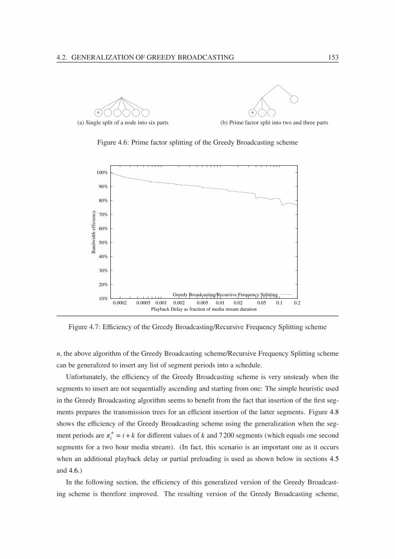
4.2. GENERALIZATION OF GREEDY BROADCASTING 153
6
(a) Single split of a node into six parts
6
(b) Prime factor split into two and three parts
Figure 4.6: Prime factor splitting of the Greedy Broadcasting scheme
10%
20%
30%
40%
50%
60%
70%
80%
90%
100%
0.0002 0.0005 0.001 0.002 0.005 0.01 0.02 0.05 0.1 0.2
Ban
dw
idth
eff
icie
ncy
Playback Delay as fraction of media stream duration
Greedy Broadcasting/Recursive Frequency Splitting
Figure 4.7: Efficiency of the Greedy Broadcasting/Recursive Frequency Splitting scheme
n, the above algorithm of the Greedy Broadcasting scheme/Recursive Frequency Splitting scheme
can be generalized to insert any list of segment periods into a schedule.
Unfortunately, the efficiency of the Greedy Broadcasting scheme is very unsteady when the
segments to insert are not sequentially ascending and starting from one: The simple heuristic used
in the Greedy Broadcasting algorithm seems to benefit from the fact that insertion of the first seg-
ments prepares the transmission trees for an efficient insertion of the latter segments. Figure 4.8
shows the efficiency of the Greedy Broadcasting scheme using the generalization when the seg-
ment periods are π+i = i+k for different values of k and 7200 segments (which equals one second
segments for a two hour media stream). (In fact, this scenario is an important one as it occurs
when an additional playback delay or partial preloading is used as shown below in sections 4.5
and 4.6.)
In the following section, the efficiency of this generalized version of the Greedy Broadcast-
ing scheme is therefore improved. The resulting version of the Greedy Broadcasting scheme,

154 CHAPTER 4. GENERALIZED GREEDY BROADCASTING SCHEME
10%
20%
30%
40%
50%
60%
70%
80%
90%
100%
0.0002 0.0005 0.001 0.002 0.005 0.01 0.02 0.05 0.1 0.2
Ban
dw
idth
eff
icie
ncy
Playback Delay as fraction of media stream duration
Unenhanced Generalized Greedy Broadcasting
Figure 4.8: Efficiency of the generalized version of the Greedy Broadcasting scheme for different
starting periods and 7200 segments
called Generalized Greedy Broadcasting scheme in the following, shows not only a steady high
efficiency, it even outperforms any transmission scheme of the frequency-based class.
In sections 4.5 to 4.11, the positive effects of this generalization are further exploited in several
application cases which partially have been proposed in chapter 3 in the context of other transmis-
sion schemes.
4.3 Efficiency Improvements
To improve the efficiency and to make the efficiency less fluctuating at the same time, the heuristic
decision of the Greedy Broadcasting scheme has to be improved: As described above, the Greedy
Broadcasting scheme takes two measurements for each node N into account when it searches the
best place for a segment #i:
1. The wasted bandwidth, measured by π+i mod ΠN and
2. the period of the node ΠN .
The Greedy Broadcasting algorithm evaluates these two measurements in this order, i. e. it first
checks which nodes provide the lowest bandwidth wastage and examines the second condition
only for the nodes which qualified equally according to the first condition.
Better results can be obtained if these two measurements are combined to a single “quality”
function. For this purpose the measurements have to be normalized and weighted: The following
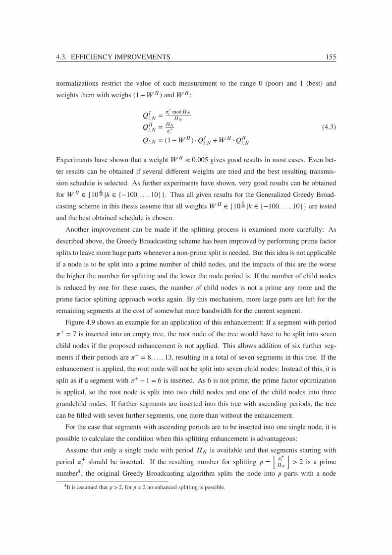
4.3. EFFICIENCY IMPROVEMENTS 155
normalizations restrict the value of each measurement to the range 0 (poor) and 1 (best) and
weights them with weighs (1−W II ) and W II :
QIi,N =
π+i modΠN
ΠN
QIIi,N
=ΠN
π+i
Qi,N = (1−W II ) ·QIi,N +W II ·QII
i,N
(4.3)
Experiments have shown that a weight W II ≈ 0.005 gives good results in most cases. Even bet-
ter results can be obtained if several different weights are tried and the best resulting transmis-
sion schedule is selected. As further experiments have shown, very good results can be obtained
for W II ∈ {10k20 |k ∈ {−100, . . . ,10}}. Thus all given results for the Generalized Greedy Broad-
casting scheme in this thesis assume that all weights W II ∈ {10k20 |k ∈ {−100, . . . ,10}} are tested
and the best obtained schedule is chosen.
Another improvement can be made if the splitting process is examined more carefully: As
described above, the Greedy Broadcasting scheme has been improved by performing prime factor
splits to leave more huge parts whenever a non-prime split is needed. But this idea is not applicable
if a node is to be split into a prime number of child nodes, and the impacts of this are the worse
the higher the number for splitting and the lower the node period is. If the number of child nodes
is reduced by one for these cases, the number of child nodes is not a prime any more and the
prime factor splitting approach works again. By this mechanism, more large parts are left for the
remaining segments at the cost of somewhat more bandwidth for the current segment.
Figure 4.9 shows an example for an application of this enhancement: If a segment with period
π+ = 7 is inserted into an empty tree, the root node of the tree would have to be split into seven
child nodes if the proposed enhancement is not applied. This allows addition of six further seg-
ments if their periods are π+ = 8, . . . ,13, resulting in a total of seven segments in this tree. If the
enhancement is applied, the root node will not be split into seven child nodes: Instead of this, it is
split as if a segment with π+− 1 = 6 is inserted. As 6 is not prime, the prime factor optimization
is applied, so the root node is split into two child nodes and one of the child nodes into three
grandchild nodes. If further segments are inserted into this tree with ascending periods, the tree
can be filled with seven further segments, one more than without the enhancement.
For the case that segments with ascending periods are to be inserted into one single node, it is
possible to calculate the condition when this splitting enhancement is advantageous:
Assume that only a single node with period ΠN is available and that segments starting with
period π+i should be inserted. If the resulting number for splitting p =
⌊π+i
ΠN
⌋> 2 is a prime
number4, the original Greedy Broadcasting algorithm splits the node into p parts with a node
4It is assumed that p > 2, for p = 2 no enhanced splitting is possible.

156 CHAPTER 4. GENERALIZED GREEDY BROADCASTING SCHEME
7
9
7
11
7
12
7
13
Π:π :+ 10
4
7
321 5 6 7
7
7
7
8
(a) Splitting the root node into seven segments gives a
transmission schedule with seven segments
11
10
12
10
13
10
14
Π:π :+ 10
4
10
1 2 3 5 6 7 8
6
7
6
8
6
9
10
(b) Splitting the root node into six segments instead al-
lows to use prime factor optimization (split by two first
and then by three) thus yielding eight segments in total
Figure 4.9: Example for increased efficiency from enhanced splitting
period p ·ΠN each. These nodes can then only be used to transmit p segments as the segment
periods do not allow further splitting. (See figure 4.9a for an example.)
But when the node is split into p− 1 parts instead (as done in figure 4.9b), the prime factor
splitting can be used because p− 1 is dividable by 2 if p > 2 is a prime. Thus this prime factor
splitting gives two nodes C1 and C2 of period 2 ·ΠN . C1 is then split further and can carry at least
p−12
nodes (the exact number may be higher ifp−1
2is not prime and prime splitting can be applied
again or if this enhanced splitting is advantageous for C1). When these parts are used up, C2 has to
be split into (at least)
⌊π+i +
p−12
2·ΠN
⌋nodes which allows to insert (at least)
⌊π+i +
p−12
2·ΠN
⌋further segments.
Therefore, the total number of inserted segments using enhanced splitting is (at least)
n ≥ p−12
+
⌊π+i +
p−12
2·ΠN
⌋
≥ p−12
+⌊π+i +ΠN
2·ΠN
⌋+
⌊p−1
2−ΠN
2·ΠN
⌋
=p−1
2+
⌊π+i
Πi+1
2
⌋+
⌊p−1
2−ΠN
2·ΠN
⌋
≥ p−12
+
⎢⎢⎢⎣⌊
π+i
Πi
⌋+1
2
⎥⎥⎥⎦+
⌊p−1
2−ΠN
2·ΠN
⌋
=p−1
2+
p+12
+
⌊p−1
2−ΠN
2·ΠN
⌋
= p+
⌊p−1
2−ΠN
2·ΠN
⌋= p+
⌊p−1−2·ΠN
4·ΠN
⌋
(4.4)
This means that decreasing the split number if it is prime yields at least the same number of
segments if p ≥ 2 ·ΠN +1 and definitively more segments if p ≥ 6 ·ΠN +1.
Even though this result cannot be generally applied if more than one node is available or the
segment periods are not continuously increasing by one, it shows that it may be beneficial to

4.4. INCREASING THE PLAYBACK DELAY 157
prohibit splitting by a large prime number. Experiments have shown that good results are gained
if prime number splits for p ≥ L ·ΠN +1 with L = 7 are prevented. Better results can be obtained
again if several different limits for the above fraction are applied and the best result is used. For
the results in this thesis, the limits L ∈ {5,7,∞} have been used.
Figure 4.10 shows the efficiency of the enhanced Generalized Greedy Broadcasting scheme
for different playback delays, once with W II = 10−4620 and L = 7 and once using the best result
from using W II ∈ {10k20 |k ∈ {−100, . . . ,10}} and L ∈ {5,7,∞}. Although this enhancement
seems to show only minor effect when compared to figure 4.7, the enhancement justifies itself
when examining the efficiency for different starting periods as shown in figure 4.11 compared to
figure 4.8.
10%
20%
30%
40%
50%
60%
70%
80%
90%
100%
0.0002 0.0005 0.001 0.002 0.005 0.01 0.02 0.05 0.1 0.2
Ban
dw
idth
eff
icie
ncy
Playback Delay as fraction of media stream duration
Generalized Greedy Broadcasting (best result)Generalized Greedy Broadcasting (single set of parameters)
Figure 4.10: Efficiency of the enhanced Generalized Greedy Broadcasting scheme
4.4 Increasing the Playback Delay
Starting with this section, several enhancements for media-on-demand transmissions are exam-
ined. Many of these enhancements are part of one of the transmission schemes which have been
proposed in chapter 3, but it is often possible to extract the mechanisms behind them and apply
the underlying techniques to other transmission schemes — including the Generalized Greedy
Broadcasting scheme — to improve the efficiency or enhance the usability.
In this section and the next section, the effect of modifying the playback delay to the re-
quired server bandwidth is examined. In general, nearly every pro-active transmission scheme

158 CHAPTER 4. GENERALIZED GREEDY BROADCASTING SCHEME
10%
20%
30%
40%
50%
60%
70%
80%
90%
100%
0.0002 0.0005 0.001 0.002 0.005 0.01 0.02 0.05 0.1 0.2
Ban
dw
idth
eff
icie
ncy
Playback Delay as fraction of media stream duration
Generalized Greedy Broadcasting (best result)Generalized Greedy Broadcasting (single set of parameters)
Figure 4.11: Efficiency of the enhanced Generalized Greedy Broadcasting scheme for different
starting periods and 7200 segments
(the Round-Robin Broadcasting scheme is an exception) supports modifications of the playback
delay: For some transmission schemes, the playback delay is strictly coupled to the duration of
the first segment and can only be modified by changing the segment sizes, but other transmission
schemes allow separate modifications to the playback delay. As a first step, all calculations in this
section assume that the playback delay is equal to the duration of the first segment (i. e. to the
slot interval). The effects of modifying the playback delay independently of the slot interval are
examined in the next following section.
4.4.1 Intention and Effects
The advantage of increasing the playback delay is that the receiver system has more time for
receiving each segment, or in other words: All segments can be transmitted less frequently which
lowers the bandwidth requirements. The bandwidth savings which are gained thereby can be
approximated from the formula for the minimum required bandwidth: If the playback delay is
increased from W + = δ to W +′ = δ′, the required bandwidth reduces by
B−b− B−′
b=(Ψ0
(d+W +
δ
)−Ψ0
(W +
δ
))−(Ψ0
(d+W + ′
δ′
)−Ψ0
(W + ′δ′
))≈ ln
(d+W +
W +
)+ γ− ln
(d+W + ′W + ′
)− γ
= ln(
d+W +
d+W + ′
)− ln
(W + ′W +
)≈ ln
(W +
W + ′
)(4.5)

4.4. INCREASING THE PLAYBACK DELAY 159
The last approximation is only valid if the media stream duration is much larger than the playback
delay.
This formula shows that an increase of the playback delay by a factor of approximately
e ≈ 2.718 (the Euler constant) reduces the bandwidth by one channel of media stream bit rate.
Figure 4.12 shows the effect of modifying the playback delay to the minimum required bandwidth,
still assuming that the slot interval is equal to the playback delay.
3
4
5
6
7
8
9
10
0 0.01 0.02 0.03 0.04 0.05
Ban
dw
idth
in
mu
ltip
les
of
med
ia s
trea
m b
itra
te
Playback delay as fraction of media stream duration
Average server bandwidth
Figure 4.12: Impact of playback delay to minimum required bandwidth
The above formulas can also be used in the reverse case to estimate the playback delay which
has to be used if only a limited amount of bandwidth is available.
4.4.2 Transmission Function for Playback Delays
As the playback function should define how much data of the media stream is required at a given
time at the receiver system (relative to a playback request), a playback delay simply shifts the
cumulative bandwidth function by the duration of the playback delay in the direction of the positive
time axis, so that the corresponding transmission function can be defined by
Tplaybackdelay(t) = t−W+
(4.6)
The resulting playback function for a playback delay is
F (t) = f (Tplaybackdelay (t))
= f (t−W +)(4.7)

160 CHAPTER 4. GENERALIZED GREEDY BROADCASTING SCHEME
where F denotes the playback function and f is the cumulative bandwidth function of the media
stream.
Figure 4.13 shows an example for a transmission function where a playback delay has been
applied to.
playback request
Maximum
Time after
Offset in transmitted data
playback−
delay
Figure 4.13: Playback function when a playback delay is in effect
4.4.3 Application to the Generalized Greedy Broadcasting Scheme
Increasing the playback delay for transmissions using the Generalized Greedy Broadcasting
scheme by increasing the segment sizes gives nearly the same results as of the bandwidth cal-
culations above. Only for very large segment sizes a higher efficiency loss emerges. A solution to
this problem is presented in the following section.
4.5 Reducing Segment Sizes
This section examines the idea of decoupling the slot interval from the playback delay. For most
transmission schemes, the slot interval for a transmission is determined by the playback delay:
After the recipient system has joined the transmission, it awaits the next slot boundary and starts
playback when the boundary is reached. (Both the network delay for joining the transmission
and a delay for compensation of network jitter are disregarded here.) Therefore, the maximum
playback delay is equal to the duration of the slot interval and the minimum playback delay is
zero.
When the transmission scheme allows to select the playback delay independently (or at least as
an integer multiple) of the slot interval, it is possible to reduce the segment size while keeping the
maximum playback delay constant. In this case, the receiver system does not start the playback
immediately when reaching the first slot boundary but after an additional playback delay.

4.5. REDUCING SEGMENT SIZES 161
4.5.1 Intention and Effects
Reducing the segment size independent of the playback delay has several advantages: Firstly, it is
possible to use a segment size which matches the requirements of the media stream, independent
of the playback delay. Secondly, the frequency-based transmission schemes perform at a higher
efficiency in the case of a long playback delay: By using a slot interval much shorter than the play-
back delay, the number of segments is increased which allows for a more fine-grained scheduling
of the segments. Thirdly, by decoupling the playback delay from the slot interval, the minimum
playback delay is increased which reduces the bandwidth requirements without an increase of the
maximum playback delay.
To demonstrate the bandwidth saving which is gained this way, a media stream of two segments
is assumed as shown in figure 4.14a. When the slot interval is halved, the maximum playback
delay would be halved at the same time, so an additional playback delay of one slot interval is
introduced as demonstrated in figure 4.14b. But according to the additional playback delay, the
even numbered halved segments can be transmitted less frequently as before, causing a bandwidth
saving of about a forth of the media stream bit rate in this example. (For better understanding, the
Harmonic Equal-Bandwidth Broadcasting scheme has been used, even if this transmission scheme
is practically unusable.)
Figure 4.15 shows the bandwidth saving which is gained by reducing the segment size for a
playback delay of 1120
of the media stream duration. Please note that the bandwidth does not
diverge towards infinity if the segment size tends to zero:
limδ→0
B−b= lim
δ→0
(Ψ0
(d+W +
δ
)−Ψ0
(W +
δ
))≈ lim
δ→0
(ln(d+W +
δ
)− ln
(W +
δ
))= ln
(d+W +
W +
)= ln
(1+ d
W +
)(4.8)
Often this formula is used to calculate the minimum required bandwidth for a media on demand
transmission (as an approximation to equation (3.9) in section 3.1.3), disregarding that the seg-
ment size may not become infinitely small.
Due to this convergence, the amount of bandwidth which can be saved by reducing the segment
size is also limited: If the slot interval is reduced from δ =W + to an infinitely small value δ′ → 0,
the bandwidth savings are
B−b− B−′
b= lim
δ→W +
(Ψ0
(d+W +
δ
)−Ψ0
(W +
δ
))− lim
δ′→0
(Ψ0
(d+W +
δ′
)−Ψ0
(W +
δ′
))≈ (ln(1+ d
W +
)+ γ)−(ln(1+ d
W +
))= γ
(4.9)

162 CHAPTER 4. GENERALIZED GREEDY BROADCASTING SCHEME
Channel #2:
Recipient:
Channel #1:
1 b
Bandwidth usageSegment #
Total
1/2 b
3/2 b
Maximum playback delay
1 1 11 11 11 1
22222
1
t21
1
2
(a) Transmission schedule with original segment size and no additional playback delay
Channel #4:
Channel #1:
Channel #3:
Recipient:
Channel #2:
Maximum playback delay
1 11 1 11 1 1 1
2 2 2 2 2
3 3 3
4 4 4
3
t21 43
4
3
2
1
1
2
3
1/2 b
1/3 b
1/4 b
4
Total
1/5 b
77/60 b
Bandwidth usageSegment #
(b) Transmission schedule with halved segment size and an additional playback delay
Figure 4.14: Example for bandwidth saving by halving the segment size
0
0.1
0.2
0.3
0.4
0.5
0.6
0 0.2 0.4 0.6 0.8 1
Ban
dw
idth
sav
ing
as
mu
ltip
les
of
med
ia s
trea
m b
itra
te
Segment duration as fraction of maximum playback delay
Average server bandwidth saving
Figure 4.15: Bandwidth saving from reduction of slot interval

4.5. REDUCING SEGMENT SIZES 163
Depending on the ratio of the playback delay to the media stream duration, the bandwidth saving
can be up to γ ≈ 0.577215665 times the media stream bit rate.
As mentioned above, the minimum playback delay increases when an additional playback delay
is introduced, thus this optimization must not be applied if the minimum (or average) playback
delay is to be minimized.
4.5.2 Transmission Function for Reduced Segment Sizes
Reducing segment sizes has no effect on the transmission function because no part of the media
stream is played back earlier or later. The change of the segment size only influences the gran-
ularity with which the resulting playback function is sampled by the transmission scheme when
splitting the media stream into segments.
4.5.3 Application to the Generalized Greedy Broadcasting Scheme
The ability to decouple the segment size from other parameters like playback delay and preloaded
amount of data (see next section) is one major advantage of the Generalized Greedy Broadcast-
ing scheme: As the Generalized Greedy Broadcasting scheme allows to specify arbitrary segment
periods when a transmission schedule is created, the segment periods can be calculated to respect
any desired playback delay up to the resolution of one slot interval5. Figure 4.16 shows the effi-
ciency of the Generalized Greedy Broadcasting scheme, once for the case that the playback delay
equals the slot interval and once if the playback delay is decoupled from the slot interval and
7 200 segments are used. It is clearly visible that the decoupling of the playback delay increases
the efficiency and removes the inefficiency peaks of long playback delays which result from bad
scheduling capabilities for low numbers of segments.
The needed segment periods can be calculated using the following formula for constant-bit-rate
media streams:
π+i = i−1+
⌊W +
δ
⌋(4.10)
The transmission of variable-bit-rate streams is examined in section 4.8 in more detail, including
a new formula for segment period calculation which takes playback delay and partial preloading
together with bandwidth variations into account.
5Although the Generalized Greedy Broadcasting scheme makes no assumption about segment sizes, it is suggested
to align them to media integral boundaries (e. g. group-of-pictures or single frames) or to the size of data units of the
lower-level protocols.

164 CHAPTER 4. GENERALIZED GREEDY BROADCASTING SCHEME
10%
20%
30%
40%
50%
60%
70%
80%
90%
100%
0.0002 0.0005 0.001 0.002 0.005 0.01 0.02 0.05 0.1 0.2
Ban
dw
idth
eff
icie
ncy
Playback Delay as fraction of media stream duration
Generalized Greedy Broadcasting (decoupled segment sizes)Generalized Greedy Broadcasting (bound segment sizes)
Figure 4.16: Comparison of Generalized Greedy Broadcasting scheme for bound and decoupled
segment sizes
4.6 Partial Preloading
This section examines a mechanism called partial preloading [PL01, Pâr02, Pâr01c, PLM99]
which has similar bandwidth savings as an increased playback delay. Partial preloading means
that a part of the media stream is preloaded to the recipient systems storage at some time before
the transmission is requested by the consumer.
4.6.1 Intention and Effects
Preloading has several impacts on the setup of the receiver system:
• The receiver system must always (or at least at the time of preloading) be activated if the
media assortment is modified and preloading has to take place.
• The receiver system must always (or at least at the time of preloading) be connected to the
network. In case of power or network failures, it may be possible that the customer cannot
view a media stream until the preloaded part has been transmitted again.
• The receiver system must reserve part of its bandwidth for the reception of the preloaded
data.
• The receiver system has to receive the preloaded parts before it can be used for the first time

4.6. PARTIAL PRELOADING 165
(i. e. after buying the system, it cannot be used immediately unless the latest version of the
preloaded parts have been stored on the system).
• The receiver system must reserve storage space for preloaded data.
But partial preloading has a lot of advantages at the same time:
• Sender and receiver bandwidth requirements for media stream transmissions are signifi-
cantly lower,
• zero-delay playback is possible, even for pro-active transmission schemes, and
• preview of the beginning of media streams is possible at any time without additional band-
width consumption or playback delay.
Theoretically, every media transmission scheme can use partial preloading by simply transmitting
some part of the media stream to the receiver system in advance and applying the transmission
scheme to the remaining part of the media stream (increasing the maximum playback delay by the
duration of the preloaded part).
As the first segments of the media stream consume the most bandwidth in a transmission,
the highest bandwidth saving is achieved if the beginning of a media stream is preloaded. More
precisely, if a part of size P of the media stream is preloaded, the minimum required bandwidth of
the non-preloaded transmission can be calculated using the following formula:
B−b= Ψ0
(d+W +
δ
)−Ψ0
(f−1(P )+W +
δ
)≈ ln
(d+W +
f−1(P )+W +
) (4.11)
Therefrom follows that the required bandwidth is reduced by partial preloading by
B−b− B−′
b=(Ψ0
(d+W +
δ
)−Ψ0
(W +
δ
))−(Ψ0
(d+W +
δ
)−Ψ0
(f−1(P )+W +
δ
))≈ ln
(d+W +
W +
)− ln
(d+W +
f−1(P )+W +
)= ln
(1+
f−1(P )
W +
) (4.12)
Figure 4.17 shows the effect of modifying the amount of preloading to the minimum required
bandwidth for a constant-bit-rate media stream transmission with different numbers of segments.
As mentioned above, partial preloading also allows for zero-delay playback. This can be iden-
tified when the minimum bandwidth formula is examined for the case that W + tends toward
0: While the bandwidth without preloading diverges to infinity, the bandwidth stays limited if
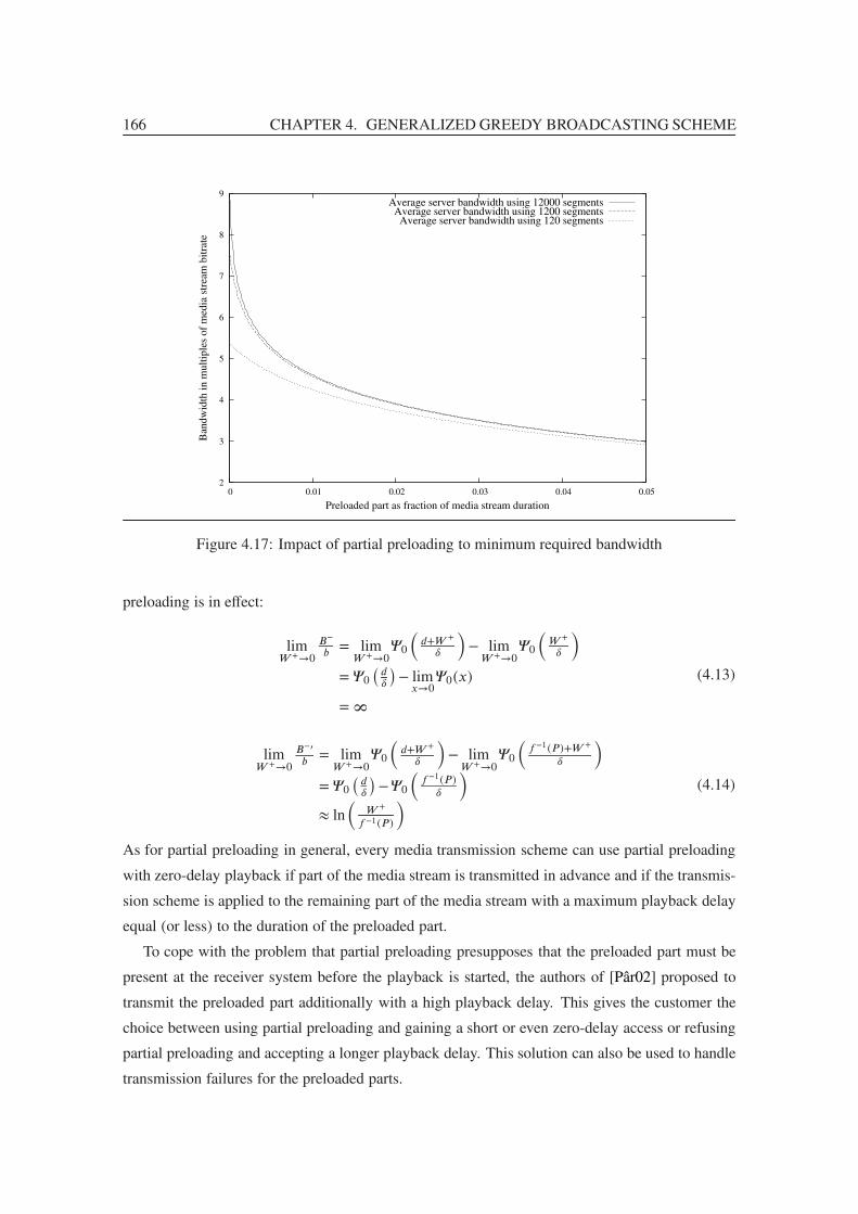
166 CHAPTER 4. GENERALIZED GREEDY BROADCASTING SCHEME
2
3
4
5
6
7
8
9
0 0.01 0.02 0.03 0.04 0.05
Ban
dw
idth
in
mu
ltip
les
of
med
ia s
trea
m b
itra
te
Preloaded part as fraction of media stream duration
Average server bandwidth using 12000 segmentsAverage server bandwidth using 1200 segmentsAverage server bandwidth using 120 segments
Figure 4.17: Impact of partial preloading to minimum required bandwidth
preloading is in effect:
limW +→0
B−b= lim
W +→0Ψ0
(d+W +
δ
)− lim
W +→0Ψ0
(W +
δ
)= Ψ0
(dδ
)− limx→0
Ψ0(x)
=∞(4.13)
limW +→0
B−′b
= limW +→0
Ψ0
(d+W +
δ
)− lim
W +→0Ψ0
(f−1(P )+W +
δ
)= Ψ0
(dδ
)−Ψ0
(f−1(P )
δ
)≈ ln
(W +
f−1(P )
) (4.14)
As for partial preloading in general, every media transmission scheme can use partial preloading
with zero-delay playback if part of the media stream is transmitted in advance and if the transmis-
sion scheme is applied to the remaining part of the media stream with a maximum playback delay
equal (or less) to the duration of the preloaded part.
To cope with the problem that partial preloading presupposes that the preloaded part must be
present at the receiver system before the playback is started, the authors of [Pâr02] proposed to
transmit the preloaded part additionally with a high playback delay. This gives the customer the
choice between using partial preloading and gaining a short or even zero-delay access or refusing
partial preloading and accepting a longer playback delay. This solution can also be used to handle
transmission failures for the preloaded parts.

4.6. PARTIAL PRELOADING 167
4.6.2 Transmission Function for Partial Preloading
Similar to a playback delay, partial preloading shifts the cumulative bandwidth function, but in a
different direction: As partial preloading modifies the amount of data which has to be transmitted
to the receiver system while leaving the playback time of any part of the media stream unmodified,
the cumulative bandwidth function is shifted in the direction of the transmission offset in the media
stream by the amount of preloaded data P :
Tpartialpreloading(p) = p−P (4.15)
The resulting playback function can be obtained the following way:
F (t) = Tpartialpreloading(f (t))
= f (t)−P(4.16)
Again, F denotes the playback function and f the cumulative bandwidth function of the media
stream.
Figure 4.18 shows an example for a playback function where partial preloading has been used.
Offset in transmitted data
Playback time
of preloaded
data
Time after
playback requestPreloaded
amount
Figure 4.18: Playback function when partial preloading is used
4.6.3 Application to the Generalized Greedy Broadcasting Scheme
Preloading a part of the media stream equal to the segment size is the simplest way to use partial
preloading with the Generalized Greedy Broadcasting scheme. But if a larger amount is to be
preloaded, the segment sizes become very large this way which causes some efficiency losses.
One way to circumvent this problem (which also occurred in the section 4.4 in the context of
increased playback delay) is to shorten the slot interval independently of the amount of preloaded
data as described in the previous section for the playback delay. The needed segment periods can
be calculated in case of partial preloading using the following formula for constant-bit-rate media

168 CHAPTER 4. GENERALIZED GREEDY BROADCASTING SCHEME
streams:
π+i = i−1+
⌊W + +f−1(P )
δ
⌋(4.17)
From this equation, it is readily identifiable that W + +f−1(P ) ≥ δ is necessary to ensure that all
segment periods are non-zero, i. e. that it is possible to create a transmission schedule.
Optional partial preloading, i. e. transmitting the preloaded part additionally with a higher
playback delay for receiver systems that do not have the preloaded parts, is also possible with
the Generalized Greedy Broadcasting scheme: As the Generalized Greedy Broadcasting scheme
allows to define an arbitrary period for each segment, any desired additional playback delay can
be applied to the segments of the preloaded part.
4.7 Introducing Breaks into Transmissions
While an additional playback delay can be seen as a break at the beginning of the playback, it is
also possible to insert breaks at any position into the media stream [PQ02]. These breaks may
be required by the broadcasting organizations to show advertisements which can be transmitted
alongside the media transmission or which have been preloaded to the receiver system.
4.7.1 Intention and Effects
Besides of commercial reasons in case of advertisements, breaks have a lowering effect on the
bandwidth requirements: The part of the media stream after the break has to be transmitted less
frequently after insertion of a break because the receiver system can use the duration of the break
for receiving further media stream data.
Unfortunately, the bandwidth requirements of later parts of a media stream transmission need
much less bandwidth than the former parts, so the saved bandwidth is the lower the later the break
is inserted. Figure 4.19 shows the bandwidth reducing effect of a break of 124
of the stream duration
(this equals a five minute break in a two hour stream) using a playback delay of 1120
of the stream
duration (this corresponds to one minute of a two hour media stream) depending on the time of
the break.
4.7.2 Transmission Function for Insertion of Breaks
Inserting breaks into a transmission has a similar effect to the playback function as a playback
delay; the only difference is that the shifting is delayed to the position of the break. Therefore, the
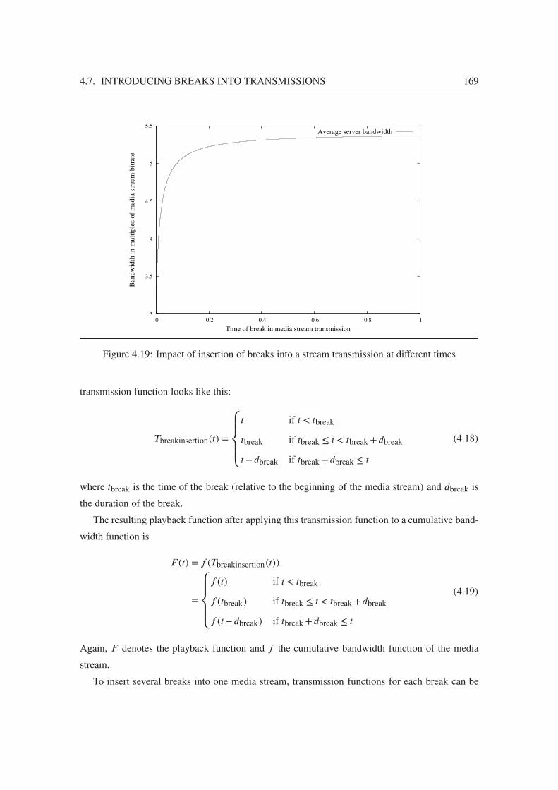
4.7. INTRODUCING BREAKS INTO TRANSMISSIONS 169
3
3.5
4
4.5
5
5.5
0 0.2 0.4 0.6 0.8 1
Ban
dw
idth
in
mu
ltip
les
of
med
ia s
trea
m b
itra
te
Time of break in media stream transmission
Average server bandwidth
Figure 4.19: Impact of insertion of breaks into a stream transmission at different times
transmission function looks like this:
Tbreakinsertion(t) =
⎧⎪⎪⎪⎨⎪⎪⎪⎩t if t < tbreak
tbreak if tbreak ≤ t < tbreak +dbreak
t−dbreak if tbreak +dbreak ≤ t
(4.18)
where tbreak is the time of the break (relative to the beginning of the media stream) and dbreak is
the duration of the break.
The resulting playback function after applying this transmission function to a cumulative band-
width function is
F (t) = f (Tbreakinsertion(t))
=
⎧⎪⎪⎪⎨⎪⎪⎪⎩f (t) if t < tbreak
f (tbreak) if tbreak ≤ t < tbreak +dbreak
f (t−dbreak) if tbreak +dbreak ≤ t
(4.19)
Again, F denotes the playback function and f the cumulative bandwidth function of the media
stream.
To insert several breaks into one media stream, transmission functions for each break can be

170 CHAPTER 4. GENERALIZED GREEDY BROADCASTING SCHEME
applied:
F (t) = f ((Tbreakinsertionk ◦ · · · ◦Tbreakinsertion1 )(t))
= f (Tbreakinsertionk (· · · (Tbreakinsertion1 (t)) · · · ))(4.20)
where Tbreakinsertion1 , . . . ,Tbreakinsertionk are transmission functions for each break, sorted by the
time of the break (i. e. Tbreakinsertion1 is the transmission function for the first break). The times of
the breaks must be specified relative to the beginning of the media stream (ignoring all breaks) if
the transmission functions are applied in this order.
Figure 4.20 shows an example for a playback function where one break has been inserted.
Break
Offset in transmitted data
playback request
Time after
Figure 4.20: Playback function with a break inserted
4.7.3 Application to the Generalized Greedy Broadcasting Scheme
Using the Generalized Greedy Broadcasting scheme, breaks can be introduced at any time by
adjusting the segment periods accordingly. If F−1 denotes the inverse of the desired playback
function6 the segment periods can be calculated by the following formula:
π+i =
⌊F−1((i−1) ·σ)
δ
⌋(4.21)
These segment periods can then be used by the Generalized Greedy Broadcasting algorithm to
create a transmission schedule which benefits from partial preloading, increased playback delay
and breaks.
Another interesting detail is, that it is still possible to derive that F−1(0) = f−1(0+P )+W + =
f−1(P )+W + ≥ δ must be fulfilled to prevent zero segment periods from the above formulas, i. e.
that the sum of the playback delay and the duration of the preloaded part must be greater than or
equal to the slot interval.
6As the playback function is a staircase function, it is not invertible in a strict mathematical sense as it is not bijective.
Assume therefore the following definition for the inverse playback function: F−1(p) = min{t |F (t) ≥ p}

4.8. VARIABLE-BIT-RATE MEDIA TRANSMISSIONS 171
4.8 Variable-Bit-Rate Media Transmissions
The transmission of variable-bit-rate media streams is an important issue because most of the me-
dia encodings used today (e. g. H.261 [Itu93a], MPEG-1 part 2 [Itu93b], MPEG-2 part 2 [Itu00],
H.263 [Itu05a], MPEG-4 part 2 [Itu04], H.264/MPEG-4 part 10 AVC [Itu05b], VC-1 [Soc06] and
many others) perform better when generating variable-bit-rate output instead of (nearly) constant-
bit-rate streams: To reduce the bandwidth as much as possible, the video compression algorithms
benefit from two facts (see also section 2.5.3):
• The frames of the media stream contain a high amount of redundancy (which can be ex-
ploited through spatial compression).
• Consecutive frames often only differ in minor parts (which is often exploited through tem-
poral compression).
Although many compression algorithms support generation of constant-bit-rate output by adapting
the compression rate on-the-fly, the result has a lower quality than a variable-bit-rate encoded
media stream of the same average bandwidth (and often even of a lower than average bandwidth):
As the media encoder has to produce the same bit rate for parts of the media stream with low
redundancy (complex frames, high motion) as for parts with high redundancy (simple frames, less
or no motion), the further ones have to be encoded with a high compression rate (loosing many
details) while the latter ones can be encoded using a low compression rate (producing a higher
quality than average for these parts).
4.8.1 Smoothing Variable-Bit-Rate Media Streams
Instead of creating constant-bit-rate output, it is possible to use variable-bit-rate streams and apply
a smoothing algorithm to them for transmission. Smoothing [SRR99, SRR04, ASS01, RR99]
of a media stream is a mechanism to convert a variable-bit-rate media stream into a constant-
bit-rate one where high bandwidth parts of the variable-bit-rate media stream are transmitted in
advance using times of lower bandwidth for compensation. The advantage of smoothing is that
the created output can be transmitted the same way as a constant-bit-rate media stream without
loss of quality or increase of the average media bandwidth. Therefore, any media-on-demand
transmission scheme can handle variable-bit-rate media streams by smoothing them beforehand.
Smoothing can benefit from the playback delay by using part of the delay for smoothing which
results in a lower smoothed media bit rate. This is esp. important for the beginning of the media
stream as no preceding part is available where high bandwidth parts can be moved to. On the
other side, lowering the playback delay this way increases the bandwidth which is needed for
the transmission in the same way as a reduction of the playback delay or the preloaded amount.

172 CHAPTER 4. GENERALIZED GREEDY BROADCASTING SCHEME
Therefore, one difficulty of smoothing is that the playback delay has to be divided optimally into
a part which is used by the transmission schedule and a part which is used for smoothing.
Figure 4.21 shows an example for smoothing a variable-bit-rate media stream transmission
which uses different amounts of the playback delay for smoothing.
using about 10% of the delay
Cumulative Decode BitrateCumulative Smoothed Bitrate
Cumulative Smoothed Bitrate
Cumulative Smoothed Bitrate
using about 90% of the delay
Preloaded
Segment #2
Segment #1
Amount
Segment #4
Segment #3
Amount of media stream data
Delay
Maximum
Playback−
t
using about 50% of the delay
Figure 4.21: Example for smoothing of a variable-bit-rate media stream
4.8.2 Piecewise Smoothing of Variable-Bit-Rate Media Streams
Using one smoothing bandwidth for the whole media stream has mainly two disadvantages:
Firstly, the smoothing bandwidth may be much higher than e. g. the average bandwidth of the
media stream which reduces the efficiency of the transmission scheme. And secondly, smoothing
increases the memory requirements at the receiver side as any part which is transmitted in advance
due to smoothing has to be stored at the receiver system. The authors of [LT95] and [SZKT96]
therefore developed heuristic algorithms to split a media stream into pieces of different bit rate
so that the bit rate within each piece remains constant and a given smoothing buffer size is not
exceeded. But even for piecewise smoothing, a compromise between a low number of bandwidth
changes and a small buffer size for smoothing has to be found.
To benefit from piecewise smoothing in case of a frequency-based transmission scheme which
cannot transmit variable-bit-rate media streams, each piece of the media stream for which a new
bandwidth has been selected has to be scheduled in a separate transmission scheme. This creates
a lot of scheduling overhead and complexity, so piecewise smoothing looses lots of its advantages
for this type of transmission schemes.

4.8. VARIABLE-BIT-RATE MEDIA TRANSMISSIONS 173
4.8.3 Immediate Transmission of Variable-Bit-Rate Media Streams
While the smoothing approaches remove the complexity of variable-bit-rate transmissions from
the transmission scheme, they have several disadvantages:
• By moving high bit rate parts of the media stream backward in time to a position of low
bit rate, the needed transmission bandwidth is increased (and therefore the efficiency of the
transmission reduced) as the former parts of a transmission are transmitted more frequently
and thus require more bandwidth than the latter parts.
• Live transmissions cannot be smoothed (if no further delay for smoothing is added) as it is
not possible to transmit any media stream data in advance, i. e. before it has been captured.
• The storage requirements at the receiver system are increased slightly by smoothing as the
earlier transmitted parts have to be stored until they are played.
To support variable-bit-rate media streams directly, the transmission scheme must be able to
create a transmission schedule which adapts to the bandwidth variations of the media stream as
much as possible. For example, the authors of [SRR99] and [LN99] proposed algorithms to calcu-
late broadcasting series for size-based transmission schemes which performs this adaption to the
bandwidth variations, the authors of [Pâr99a] proposed bandwidth calculations for the bandwidth-
based Cautious Harmonic Broadcasting scheme and the authors of [LN00] for the bandwidth-
based Staircase Broadcasting scheme.
4.8.4 Application to the Generalized Greedy Broadcasting Scheme
Using the inverse playback function F−1, the maximum period for segment #i of a variable-bit-rate
media stream can be calculated as follows:
π+i = min
0≤x≤σ
⌊F−1((i−1)σ +x)− x
β
δ
⌋(4.22)
This function calculates the maximum period of a segment by examining each offset within the
segment and using the minimum of the calculated periods. This minimum search is necessary
to prevent that a buffer underflow happens within a segment at the receiver system: Even if the
beginning of a segment arrives just-in-time, it is not guaranteed that all data of the segment is
received when it is needed due to the bit rate variations within the segment. By searching the
minimum period for every stream offset of the segment, the segment period is adjusted accordingly.
As the Generalized Greedy Broadcasting scheme allows defining an arbitrary sequence of non-
descending segment periods when generating a transmission schedule, the above formula suffices
to create a schedule which can be used to transmit the media stream in an efficient way. Figure 4.22

174 CHAPTER 4. GENERALIZED GREEDY BROADCASTING SCHEME
shows an example transmission of the beginning of a variable-bit-rate transmission together with
the needed segment periods for the same transmission.
Playback−
Slot Duration
Preloaded
Segment #2
Segment #1
Amount
Segment #4
Segment #3
Amount of media stream dataCumulative Decode BitrateCumulative Receive Bitrate
Segment # Segment Period
1
2
3
4
3
5
5
9
Delay
t
Maximum
Figure 4.22: Example for a variable-bit-rate transmission using the maximum possible segment
period for each segment
To verify the results for adapting to a variable-bit-rate media stream instead of smoothing to
constant-bit-rate, several publicly available video traces [FR01] have been used. To get com-
parable results, all video traces have been extended to two hours. Additionally, a playback de-
lay of 60 seconds has been assumed to make smoothing possible. Table 4.1 shows the addi-
tional bandwidth requirements of the video traces for three transmission methods (Fixed-Delay
Pagoda Broadcasting and Generalized Greedy Broadcasting, both using a smoothed version of the
variable-bit-rate media stream, and the Generalized Greedy Broadcasting using the variable-bit-
rate media stream directly) relative to the theoretical minimum of the bandwidth for the transmis-
sion.
Although the results for the smoothed video streams show strong variations (between 11%
and 53% more bandwidth than the theoretical minimum) a significant decrease of the bandwidth
requirements is achieved when the Generalized Greedy Broadcasting scheme is applied to the
variable-bit-rate media stream: While the average bandwidth requirement for the smoothed media
streams lies 25% above the theoretical minimum, it is less than 1% away from the theoretical
minimum for all examined video traces when using the variable-bit-rate media stream directly.

4.9. IMMEDIATE SEGMENT RECEPTION 175
Additional Additional Additional
Media name Bandwidth Bandwidth Bandwidth
(smoothed, (smoothed, (VBR,
FDPB) GGB) GGB)
Aladdin +40.7% +36.0% +0.4%
Die Hard (III) +26.9% +23.3% +0.3%
From Dusk till Dawn +22.9% +18.6% +0.4%
Jurassic Park +24.0% +20.2% +0.3%
Mr. Bean +27.0% +22.8% +0.4%
Robin Hood +32.8% +28.8% +0.2%
Silence of the Lambs +57.0% +52.9% +0.5%
Simpsons +14.2% +11.3% +0.2%
South Park +17.9% +14.4% +0.5%
Star Trek, First Contact +36.9% +30.9% +0.5%
Star Wars IV +27.7% +21.4% +0.7%
Starship Troopers +25.2% +21.0% +0.4%
The Firm +27.8% +22.0% +0.7%
Average +29.3% +24.9% +0.4%
Table 4.1: Bandwidth requirements for transmission of variable-bit-rate media streams compared
to theoretical minimum
4.9 Immediate Segment Reception
For the Polyharmonic Broadcasting scheme (see section 3.6.4), the authors introduced a fixed-
wait policy to circumvent a design error of the Harmonic Broadcasting scheme (see section 3.6.1).
This fixed-wait policy requires that the reception is started immediately when the channels are
joined instead of delaying the reception until the next segment boundary is reached7 and starting
the playback after a fixed delay instead when reaching the next segment boundary.
4.9.1 Intention and Effects
Joining an ongoing transmission immediately has the advantage that it is assured that a segment
has been completely received after a delay equivalent to the segment period, even if the bandwidth
of the transmission channel is lower than the media bit rate. (This is the way how the Polyharmonic
Broadcasting scheme works around the problem of the Harmonic Broadcasting scheme.) But the
same advantage can also be used in other cases where the bandwidth of the transmission channel
is (permanently or temporarily) lower than the media bit rate, e. g. when transmitting a variable-
bit-rate media stream as explained in the previous section. Figure 4.23 shows an example of the
same frequency-based transmission of a variable-bit-rate media stream as in section 4.8, this time
7Strictly speaking, it is not possible to join an ongoing transmission immediately, at least delays from link layer
access (e. g. tuning to the right satellite frequency), routing (e. g. IGMP group join delays) and packetization (for
packet-based protocols) must be accepted. If these delays are added to the maximum playback at a later stage, they can
be ignored here for improved comprehension.

176 CHAPTER 4. GENERALIZED GREEDY BROADCASTING SCHEME
utilizing immediate receptions: As segments are never received concurrently to their playback in
this case, the cumulative receive bandwidth is a staircase function (figure 4.23b shows the result of
the immediate reception compared to figure 4.23a with delayed reception). This allows to increase
the segment period for some segments (as illustrated in figure 4.23c).
The only disadvantage of immediately receiving data instead of awaiting the next segment
boundary is a gain of a little bit more complexity, slightly higher storage requirements and an
increase of the minimum playback delay up to the maximum playback delay.
If the bandwidth of the transmission channels equal the media bit rate (e. g. when a constant-
bit-rate media stream is transmitted using a typical frequency-based transmission scheme) starting
the reception immediately has no advantages as the data is delivered with the same rate as it is
consumed.
4.9.2 Application to the Generalized Greedy Broadcasting Scheme
The Generalized Greedy Broadcasting scheme benefits from immediate segment receptions for
variable-bit-rate transmissions as it allows lowering of segment periods in some cases. Even the
complexity of the segment period calculation is lowered when immediate segment receptions are
allowed: The maximum period for segment #i can then be calculated by:
π+i =
⌊F−1((i−1) ·σ)
δ
⌋(4.23)
Compared to equation (4.22) of section 4.8, this formula lacks the minimum search as it is suffi-
cient in this case to check if the beginning of a segment arrives just-in-time.
4.10 Decoupled Channel-Bandwidth
Most of the frequency-based transmission schemes require that the channel bandwidth equals the
media bit rate. Although this makes the transmission scheme more simple, it may not fit to existing
environments, e. g. if the network provides channels of fixed bandwidth or if the total available
bandwidth is not an integer multiple of the media bit rate.
4.10.1 Intention and Effects
In these cases, selecting an arbitrary channel bandwidth according to the network and indepen-
dent of the media bit rate helps to utilize the full network bandwidth. Theoretically, any channel
bandwidth is possible as long as the resulting maximum period for the first non-preloaded seg-
ment is non-zero. But practically, a low channel bandwidth prohibits a fine-grained scheduling of
segments as the slot interval increases (assuming that the segment size is kept constant).

4.10. DECOUPLED CHANNEL-BANDWIDTH 177
tPreloaded
Segment #2
Segment #1
Amount
Segment #4
Segment #3
Amount of media stream dataCumulative Decode BitrateCumulative Receive Bitrate
Delay
Maximum
Playback−
Slot Duration
(a) Transmission with delayed reception
Playback−
Slot Duration
Preloaded
Segment #2
Segment #1
Amount
Cumulative Decode BitrateCumulative Receive Bitrate
Amount of media stream data
Segment #4
Segment #3
Delay
t
Maximum
(b) Transmission with immediate reception but unmodified segment periods
t
Cumulative Decode BitrateCumulative Receive Bitrate
Preloaded
Segment #2
Segment #1
Amount
Segment #4
Segment #3
Amount of media stream data
Delay
Maximum
Playback−
Slot Duration
(c) Transmission with immediate reception when segment periods are increased
Figure 4.23: Example for bandwidth saving by starting reception immediately

178 CHAPTER 4. GENERALIZED GREEDY BROADCASTING SCHEME
accordingly, so the total bandwidth requirements stay the same (apart from rounding errors in the
period calculation).
4.10.2 Application to the Generalized Greedy Broadcasting Scheme
As the Generalized Greedy Broadcasting scheme supports variable-bit-rate media streams directly,
it does not rely on the media stream bit rate for channels. The segment periods have to be calcu-
lated in this case in the same way as for variable-bit-rate media streams.
If channels of high bandwidth are used and the receiver systems are able to receive all channels
at once, no significant advantage is measured for the Generalized Greedy Broadcasting scheme as
it already operates near the theoretic limit.
Nevertheless, decoupling the channel bandwidth may be beneficial when the maximum receiver
bandwidth is not an exact multiple of the media bit rate (see also section 4.18) and a decoupling
of the channel bandwidth from the media bit rate may be advantageous if the channel bandwidth
cannot be modified.
4.11 Channel Sharing
When the segment size and playback function are specified in advance, it is the normal case that
the transmission scheme used does not consume all needed channels completely. This section
covers topics how the remainders of partially used channels can be utilized.
4.11.1 Intention and Effects
The unused bandwidth of the last channel may be used for several purposes (e. g. transmission of
media stream beginnings for partial preloading, preloading of commercials for breaks, software
updates, electronic program guides or other non-real-time services), but the authors of [PCL99b]
suggested that channel may be shared among several transmissions so this bandwidth can still be
used for media-on-demand transmissions.
Unfortunately, sharing channels raises several problems, esp. for frequency-based transmission
schemes:
• The receiver system has to identify the media streams on the shared channel so it can discard
any data from foreign transmissions.
• The channel parameters (segment size, channel bandwidth) must be equal for all transmis-
sions which use the shared channels to allow an efficient sharing.
• In some cases, it may be necessary that more than one shared channel has to be used for
a single transmission (e. g. if three transmission schemes all need two thirds of a channel,

4.11. CHANNEL SHARING 179
one of them has to use the leftover parts of the others). This has to be considered when
determining the receiver system bandwidth requirements.
• When a new schedule is created, the free slots of the shared channel have to be known. As
a consequence, transmission schedules cannot be generated in advance but must be created
at media startup.
• Additionally, a fragmentation problem might occur after some media allocations and re-
leases, comparable to the fragmentation problems of dynamic heap memory allocation. A
channel compaction algorithm may resolve this issue but must take care not to disrupt on-
going transmissions.
Some of these problems are relatively simple to solve, others — depending on the transmission
scheme — much more difficult:
• To distinguish several transmissions on a shared channel, different addresses (or media
stream identifiers if addressing within a channel is not supported by the lower layer pro-
tocols) can be used for each transmission.
• Using equal segment sizes and bandwidths for all transmissions is no problem if the trans-
mission scheme supports that the segment size can be selected independently from the play-
back delay and that the channel bandwidth can be chosen independently from the media
stream bit rate.
• The increase of the receiver system bandwidth has to be taken into account. If the receiver
systems do not support a higher bandwidth, channel sharing has to be limited accordingly.
For the last two problems, a better solution is provided below.
4.11.2 Application to the Generalized Greedy Broadcasting Scheme
One way to apply channel sharing to the Generalized Greedy Broadcasting scheme is to gener-
ate a schedule which exactly consumes the holes of the currently active transmissions. But this
procedure has two big disadvantages: Firstly, the unused parts of the transmission schedule are dis-
tributed across several channels which make it difficult to utilize them by other schedules without
increasing the receiver bandwidth requirements too much. Secondly, when the active transmission
terminates, segments from later started transmissions still allocate some segment positions in the
transmission schedule and prevent that the schedule can be torn down. As a result, the next trans-
mission schedule has to align itself with the remaining tree structure of the previous transmission
which typically results in a worse efficiency.
As a solution, it is advisable to put a fixed structure on the last channel (e. g. split it into a num-
ber of equally sized subtrees) and modify the schedule generating algorithm in such a way that as

180 CHAPTER 4. GENERALIZED GREEDY BROADCASTING SCHEME
few parts of the last channel are used as possible when the transmission scheme is generated. This
way, the “holes” are forcibly combined to the unused parts where they can simply be exchanged
by parts from other schedules which have been created in the same way. Another advantage of
this procedure is that the transmission schedule generation is decoupled from active transmissions
so the schedule can still be generated in advance.
4.12 Enhanced Startup
A topic which has been paid very little attention to in recent pro-active transmission scheme de-
velopment is startup and termination of media-on-demand transmissions. This section provides
an algorithm for enhancing the startup of the Generalized Greedy Broadcasting scheme which can
also be applied to other frequency-based schemes.
4.12.1 Intention and Effects
When a media transmission is started, all segments of the media stream are transmitted in the order
which is defined by the transmission schedule. An interesting fact at startup is that some segments
are transmitted this way although no receiver system will use them8: If a segment is transmitted at a
period lower than necessary, it is possible that the segment is received twice by the receiver system
before it is played9. While, at a later stage of a transmission, none of the segment transmissions
can be omitted without disrupting possibly ongoing transmissions, it is possible to leave out the
first of these broadcasts at the beginning of a newly started media stream transmission. Figure 4.24
shows an example where the transmission of segment #14 can be omitted once at media startup
without destroying the continuity of any playback.
Although an examination of Generalized Greedy transmission schedules shows that only very
few segment transmissions can be dropped this way (e. g. none of the 1 572 segments of a trans-
mission schedule for eight channels and only two out of the 11 936 segments of a schedule for
ten channels), this approach shows its full benefits when applied to transmission schedules which
have been prepared accordingly.
8In this thesis, it is assumed that the receiver systems always try to receive only the latest transmission of a segment.
Another approach would be to store any received segment, even if the transmission schedule would guarantee that
the segment is transmitted in due time again. Although the latter approach provides a lower loss probability for these
segments, it is not examined further as the loss probability is only decreased for a limited number of segments and
only for a low number of receiver systems, so this effect is barely utilizable (see section 5.1 for better error correction
schemes). Another disadvantage is an increase of the storage requirements when segments are stored prematurely.9Although a transmission with a lower period means that the transmission scheme is non-optimal, it is the common
case for most of the segments: For example, only about 17 % of all segments of a Generalized Greedy Broadcasting
transmission schedule using eight channels are scheduled with their maximum period.

4.12. ENHANCED STARTUP 181
Recipient #3:
Channel #1:
Channel #4:
Recipient #2:
Channel #3:
Channel #2:
Recipient #1:
Recipient #4:
1 1
5 10 12 14
1 1 1 1 1 1 11 1 1 1 1 1 1 11 1
515 105
t1412 525
2 4 82 2 4 162 2 4 82 2 4 172 2 4 82
9 3 187 3 6 22 3 97 3 6 19 3 237 3 63 6
1311 20 24 1311 21 15
20761 2 3 54 15148 9 1110 1312 1716 18 19
761 2 3 54 15148 9 1110 1312 1716 18 19
761 2 3 54 15148 9 1110 1312 1716 18
761 2 3 54 15148 9 1110 1312 1716
1
(a) The first transmission of segment #14 can be omitted
4
4
8
88
16
16
16
17
3
3
1
3 3
6
6 7
6 9
9
9 9
18
18
18
19
18
22
18
23
1
5
5
5
10
11
10
10
5
10
13
10
12
5
15
25
15
24
15
15
5
10
20
20
20
21
10
14
1
1
2
2
1
2
4
(b) Transmission trees of the used schedule
Figure 4.24: Example showing that it is possible to leave out a segment transmission at media
startup without interfering with any receptions
4.12.2 Modifying Transmission Schedules
One way to get transmission schedules which allow leaving out more segments at startup is to
modify the transmission schedule algorithm of the Generalized Greedy Broadcasting scheme, e. g.
the quality function which is responsible for the placement of the segments in the transmission
trees. Although this approach allows creating transmission schedules where more segments can
be left out at startup, the long term efficiency of the Generalized Greedy Broadcasting scheme
182 CHAPTER 4. GENERALIZED GREEDY BROADCASTING SCHEME
is lowered for a short term startup enhancement. For this reason, another approach is proposed
here which enhances the startup of a previously created, frequency-based transmission schedule
without changing its (long-term) efficiency.
To enhance the startup of a transmission schedule it is important to identify the condition when
a segment transmission can be left out. The basic principle has already been stated above: The first
transmission of a segment can be left out if all receivers get the segment twice before they need it
for playback, i. e. if segment #i is received twice within the first π+i slot intervals. As segment #i
is transmitted at t = φi · δ the first time and at t = (φi + πi) · δ the second time, this means, the
algorithm has to move as many segments as possible in such a way that φi+πi < π+i is satisfied
for them.
To preserve the efficiency of the transmission scheme, only a limited number of modifications
are allowed. The proposed algorithm actually only uses the following two transformations:
T1 Exchange of segments of the transmission trees if the periods of all affected nodes are less
than or equal to the required periods of the newly assigned segments10.
T2 Exchange of (sub)trees if the period of their root nodes are equal.
With these basic principles in the mind, the enhancement algorithm works the following way:
As a first step, it extracts the interior structure of the transmission schedule, i. e. for each node
of the tree representation of the transmission schedule, the node period and the number of child
nodes are fetched and saved.
In a second step, the transmission schedule is rebuilt from scratch, using only the extracted
information and the list of segments and their required periods. This step works like assembling
pieces of a puzzle: The algorithm starts with empty trees (one for each channel) and re-inserts all
segments into them in ascending order. To find the best position where a segment is inserted, the
algorithm tries every possible leaf node in the trees which can be constructed using the (remaining)
extracted information pieces about the former structure of the trees. Thereby, it assembles the
extracted information pieces using the following rules:
1. Only a piece with period “1” can be used as root of a tree.
This is necessary according to transformation T2 for the whole tree.
2. A piece can only be the root of the subtree if its period matches the period of the position
where it is inserted.
This is necessary according to transformation T2 for a subtree.
10This transformation requires that both the needed and utilized period is known for all segments. While the utilized
periods can be extracted from the transmission schedule even if the playback function of the media stream is not known
any more, the required periods have to be provided additionally.

4.12. ENHANCED STARTUP 183
3. Each node must have exactly the number of child nodes as defined in the information piece
which has been assigned to it.
This is necessary according to transformation T2, only a whole subtree may be exchanged.
4. A segment can only be assigned to a leaf node, i. e. the associated piece must define that
the node has no children. The period of the node must additionally be less or equal to the
required period of the segment.
This is a direct implication of transformation T1.
5. Each piece must be used exactly once in all trees together.
Transformations T1 and T2 only allow exchanges of segments or (sub)trees, so omissions
and duplications are not allowed.
This yields a non-empty11 list of positions N where segment #i can be inserted. From this list,
a node N is selected according to the following rules:
Let P ={N ∈N
∣∣ΦN +ΠN < π+i
}be the list of segment positions so that segment #i can be
placed in such a way that its first transmission can be omitted.
1. If P �= ∅, select (one of) the node(s) of this set which provides the latest segment transmis-
sion, i. e. N ∈ argmaxM∈P
(ΦM +ΠM ).
2. If P = ∅, select the node with the latest segment transmission of all possible nodes, i. e.
N ∈ argmaxM∈N
(ΦM +ΠM ).
Thereafter the selected node N is realized in the trees, the segment is assigned to the leaf node
and the algorithm continues with the next segment.
If the first of the above alternatives for the position of a segment has been selected, the segment
has been put at a position where it can be left out at its first transmission, if the second one has
been selected, it cannot be left out. The maximum conditions in both alternatives are used to leave
better positions for the remaining segments if possible.
Figure 4.25 demonstrates the application of the algorithm to a transmission schedule using
three logical channels. The alternative positions for each segment have been plotted into the figure
using dashed lines.
4.12.3 Improved Startup Enhancement Algorithm
The startup enhancement algorithm can even be improved further if the segments are inserted in
two rounds in the transmission trees: In the first round, only segments are inserted which can be
11It is always possible to complete the trees as the used information has been extracted from a valid construction
and the periods are kept the same for each subtree. The segments can always be assigned to the leaf nodes as they are
inserted in ascending order, i. e. even if a segment uses a leaf node with a lower period than originally, it is assured that
the segment which previously occupied the leaf node has already been assigned to another node.

184 CHAPTER 4. GENERALIZED GREEDY BROADCASTING SCHEME
3
3
1
3
6
6 7
6
3
98
6 6
1
1
2
2
4
4
1
2
4
5
(a) Original transmission trees
2 2 3 3
3 4 4 6 6 6 6
111
(b) Extracted information
1
1 11
Π+Φ:Π+Φ<π:Selected:
1 1
1
no
1
no
1
no
(c) Insertion of first segment
1 11
Π+Φ:Π+Φ<π:Selected:
2
2
2
2
2
2
2
2
2
no
2
no
3
no
3
no
1
(d) Insertion of second segment
1
2
2
Π+Φ:Π+Φ<π:Selected:
3
3
3
3
3
3
5
no
43
nono
1
1 1
(e) Insertion of third segment
2
1
2 3
2
4 4
3
Π+Φ:Π+Φ<π:Selected:
4
no
6
no
1
1 1
4 4
(f) Insertion of fourth segment
2
1
2 3
2
5 4
3
Π+Φ:Π+Φ<π:Selected:
4
yes
1
1 1
4 4
(g) Insertion of fifth segment
1
2
6 6
3 3
2
5 4 6 66
3
Π+Φ:Π+Φ<π:
9
no
Selected:
6
7
no
6
no
10
no
1
1 1
3
6 64 4
2
(h) Insertion of sixth segment
yes
1
1 1
3
6 64 4
2
1
2
6 6
3 3
2
5 4 7 67
3
Π+Φ:Π+Φ<π:
9
no
Selected:
7
7
no
6
(i) Insertion of seventh segment
1
2
6 6
3 3
2
5 4 7 68
3
Π+Φ:Π+Φ<π:
9
no
Selected:
8
7
yes
1
1 1
3
6 64 4
2
(j) Insertion of eighth segment
1
2
9
6 6
3 3
2
5 4 7 68
3
Π+Φ:Π+Φ<π:
9
no
Selected:
1
1 1
3
6 64 4
2
(k) Insertion of ninth segment
2
9
6 6
3 3
2
5 4 7 68
3
1
1 1
3
6 64 4
2
1
(l) Resulting transmission trees
Figure 4.25: Example showing functioning of the startup enhancement algorithm

4.12. ENHANCED STARTUP 185
positioned in such a way that they can be left out at their first transmission, i. e. the segments for
which it is possible to apply the first alternative of the above description. In a second round the
remaining segments are inserted. This enables the remaining segments to catch better positions
and therefore increases the number of segments which can be dropped at their first transmission.
When using two rounds, it is important to observe that the remaining segments can be inserted
into the transmission trees in the second round: As the segments are not inserted in ascending
order any more (and therefore not in ascending order of their required periods), it is possible that
segments of the first round occupy the positions in the trees which are needed for segments of the
second round.
This problem can be solved if a lower bound for the period is applied when the best position
for a segment is searched. To keep track of the positions which are needed for the segments in
the second round, two lists have to be maintained by the algorithm: The first list contains the
required periods of all segments which have been rejected in the first round, sorted in ascending
order. The second list enumerates the periods of the free leaf nodes, i. e. the periods of the leaf
node information pieces, sorted in ascending order, too. It is obvious that each element of the first
list must be greater than or equal to its corresponding element of the second list and that these
relations guarantee that all rejected segments can be inserted into the trees in the second round. To
prevent that removal of an element from the second list destroys this condition, one can try which
of the elements can be removed to find the allowed periods. A more simple approach is to remove
the first element of the second list and match the remaining elements to the elements of the first
list. The last element in the second list which violates the relation then gives the lower bound for
the period for the insertion. Figure 4.26 shows an example how this lower bound search works
when a position for the seventh segment of the example of figure 4.25 is searched.
Order of examination
Periods of remaining
Required periods
of segments:1 2 3 4 6 7
information nodes:
Required period is
greater than or equal
to node’s period, try
left.
next element on the
Required period is
less than node’s
period, found lower
bound (6)!
First element is
removed/ignored
by this algorithm
1 632 4 66 6
Figure 4.26: Example for determining the lower bound for a segment to be inserted
Figure 4.27 shows the results of both the simple and two rounds variants of the enhancement
algorithm for a four channel transmission scheme.
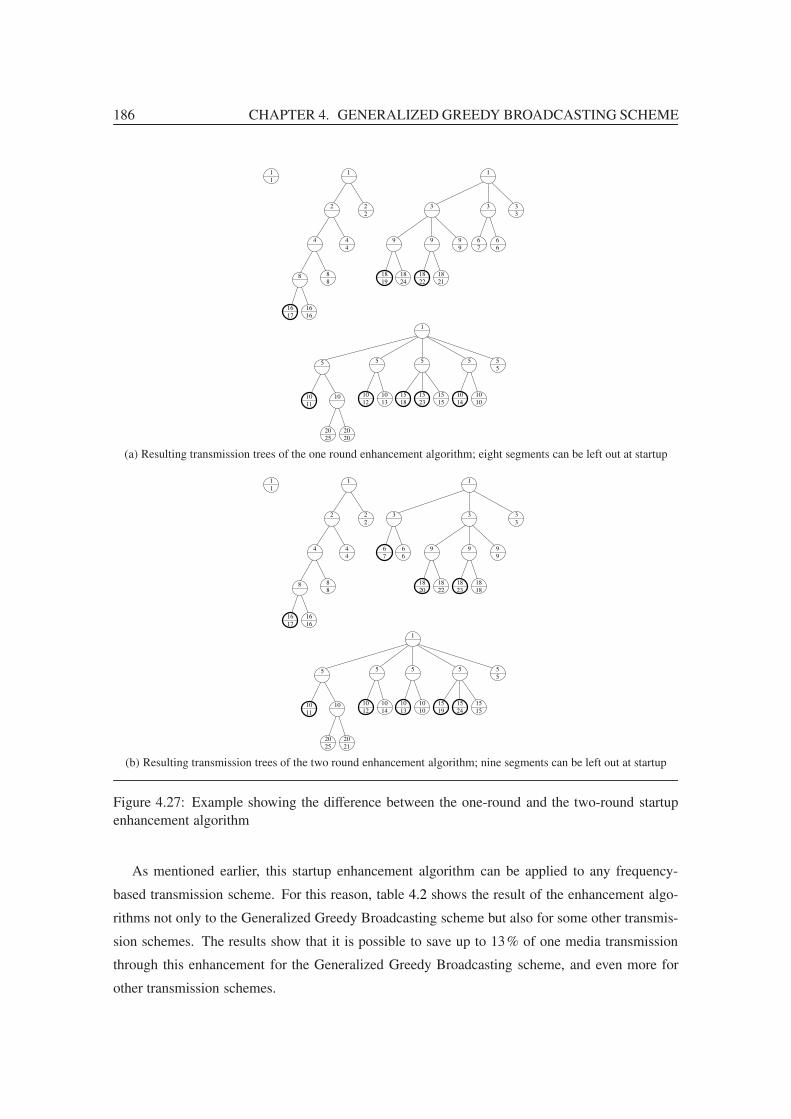
186 CHAPTER 4. GENERALIZED GREEDY BROADCASTING SCHEME
1
5
10
14
10
10
5
5
12
10
5
13
10 15 15
23
15
15
5
1
10
11
10
20
25
20
5
21
20
18
1
1
8 8
8
16
1617
16
4 4
4
2 2
2
1
18
19 24
18 18
22
18
99
3 3 3
3
6
67
69
9
(a) Resulting transmission trees of the one round enhancement algorithm; eight segments can be left out at startup
24
1
1
1
8 8
8
16
1617
16
4 4
4
2 2
2
1
3
3
5
5
12
10
5
1010
11
10
20
25
20
21
5
3
6
67
6
18 18 18 18
18
99
3
9
9
20 22 23
14
1
5
10 10
10
15 15 15
15
5
13 19
(b) Resulting transmission trees of the two round enhancement algorithm; nine segments can be left out at startup
Figure 4.27: Example showing the difference between the one-round and the two-round startup
enhancement algorithm
As mentioned earlier, this startup enhancement algorithm can be applied to any frequency-
based transmission scheme. For this reason, table 4.2 shows the result of the enhancement algo-
rithms not only to the Generalized Greedy Broadcasting scheme but also for some other transmis-
sion schemes. The results show that it is possible to save up to 13% of one media transmission
through this enhancement for the Generalized Greedy Broadcasting scheme, and even more for
other transmission schemes.

4.12. ENHANCED STARTUP 187
Saved b/w Saved b/w
Broadcasting Protocol by omitting when using
segments at proposed
startup algorithm
Fast Broadcasting:
N=4, n=15 0 %/73.3 % 73.3 %
N=6, n=63 0 %/90.5 % 90.5 %
N=8, n=255 0 %/96.9 % 96.9 %
Greedy Broadcasting:
N=4, n=26 3.8 % 26.9 %
N=6, n=203 0.5 % 21.2 %
N=8, n=1 563 0.3 % 14.3 %
New Pagoda:
N=4, n=26 0.0 % 30.8 %
N=6, n=172 3.5 % 27.7 %
N=8, n=1 166 2.0 % 17.4 %
Fixed Delay Pagoda
Broadcasting:
N=2, W +=100δ, n=568 1.9 % 17.1 %
N=4, W +=20δ, n=802 2.9 % 20.7 %
N=6, W +=10δ, n=2 367 1.3 % 14.7 %
Generalized Greedy
Broadcasting:
N=2, W +=100δ, n=609 0.7 % 13.0 %
N=4, W +=20δ, n=1 028 0.0 % 9.9 %
N=6, W +=10δ, n=4 022 0.7 % 7.8 %
Table 4.2: Amount of saved bandwidth of the first media transmission
4.12.4 Lowering the Efficiency to Improve the Startup
The reason why some transmission schemes benefit more from the startup enhancement algorithm
than others (esp. than the Generalized Greedy Broadcasting scheme) is the high efficiency of
these transmission schemes: The worse the efficiency of a transmission scheme is, the higher is
the difference between the required period and the utilized period for the segments, and the higher
this difference is, the higher is the probability to find a position where the segment can be left out
in the first transmission. This raises the question if it is possible to improve the startup further by
reducing the efficiency artificially, e. g. by lowering the required period for some segments when
a transmission schedule is created.
It is interesting to note in this context is that the bandwidth gain when suppressing a segment
transmission at startup is independent of the segment period: A segment with a high period gives
the same bandwidth savings at startup as a segment with a low period, in both cases one segment
transmission can be omitted at startup. This is a main difference to the bandwidth requirements of
the continuous transmission where the average bandwidth requirements for the transmission of a
segment are inversely proportional to the utilized period of the segment. As a consequence, it is

188 CHAPTER 4. GENERALIZED GREEDY BROADCASTING SCHEME
sufficient to decrease the period of the later segments of the transmission so the total bandwidth
requirements are nearly uneffected.
Table 4.3 shows the bandwidth requirements of a transmission with 7 200 segments and a play-
back delay of 60 slot intervals for different artificially reductions of the segment periods. As this
table shows, bandwidth increase (i. e. efficiency loss) from the reduction of periods is very minor
(less than 0.1 % in most cases), the number of omissable segments can be increased significantly.
Nevertheless, it is important to recognize that the efficiency loss will outweigh the additional sav-
ings for long-term transmissions. The last column in the table indicates this time in multiples of
the media stream duration.
First Amount of Average b/w Percentage of Number of Percentage of Number of
segment period requirements bandwidth omissable omissable transmissions
with reduction in multiples increase segments segments where segment
lowered of media at startup at startup omissions outweigh
period bit rate b/w increase
— 0 4.827136 0.00% 221 3.1% —
1 200 1 4.827880 0.02% 305 4.2% 15.7
1 200 2 4.828569 0.03% 366 5.1% 14.1
1 200 5 4.830575 0.07% 502 7.0% 11.3
1 200 10 4.834049 0.14% 653 9.1% 8.7
1 200 20 4.840500 0.28% 857 11.9% 6.6
2 400 1 4.827407 0.01% 274 3.8% 27.2
2 400 2 4.827677 0.01% 324 4.5% 26.4
2 400 5 4.828707 0.03% 443 6.2% 19.6
2 400 10 4.830060 0.06% 570 7.9% 16.6
2 400 20 4.832975 0.12% 746 10.4% 12.5
3 600 1 4.827271 0.00% 262 3.6% 42.2
3 600 2 4.827406 0.01% 304 4.2% 42.7
3 600 5 4.827858 0.01% 387 5.4% 31.9
3 600 10 4.828535 0.03% 482 6.7% 25.9
3 600 20 4.830194 0.06% 624 8.7% 18.3
4 800 1 4.827203 0.00% 249 3.5% 58.0
4 800 2 4.827271 0.00% 275 3.8% 55.6
4 800 5 4.827474 0.01% 326 4.5% 43.1
4 800 10 4.827924 0.02% 389 5.4% 29.6
4 800 20 4.828610 0.03% 480 6.7% 24.4
Table 4.3: Effects of lowering segment periods artificially to enhance startup
4.13 Enhanced Termination
After enhancing the startup of media-on-demand transmissions, this section discusses the media
termination. Similar to the startup, it is possible to save bandwidth by enhancing it.
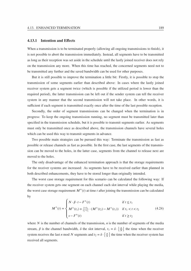
4.13. ENHANCED TERMINATION 189
4.13.1 Intention and Effects
When a transmission is to be terminated properly (allowing all ongoing transmissions to finish), it
is not possible to abort the transmission immediately. Instead, all segments have to be transmitted
as long as their reception was set aside in the schedule until the lastly joined receiver does not rely
on the transmission any more. When this time has reached, the concerned segments need not to
be transmitted any further and the saved bandwidth can be used for other purposes.
But it is still possible to improve the termination a little bit: Firstly, it is possible to stop the
transmission of some segments earlier than described above: In cases where the lastly joined
receiver system gets a segment twice (which is possible if the utilized period is lower than the
required period), the latter transmission can be left out if the sender system can tell the receiver
system in any manner that the second transmission will not take place. In other words, it is
sufficient if each segment is transmitted exactly once after the time of the last possible reception.
Secondly, the order of segment transmissions can be changed when the termination is in
progress: To keep the ongoing transmission running, no segment must be transmitted later than
specified in the transmission schedule, but it is possible to transmit segments earlier. As segments
must only be transmitted once as described above, the transmission channels have several holes
which can be used this way to transmit segments in advance.
Two possible main strategies can be pursued this way: Terminate the transmission as fast as
possible or release channels as fast as possible. In the first case, the last segments of the transmis-
sion can be moved to the holes, in the latter case, segments from the channel to release next are
moved to the holes.
The only disadvantage of the enhanced termination approach is that the storage requirements
for the receiver systems are increased: As segments have to be received earlier than planned in
both described enhancements, they have to be stored longer than originally intended.
The worst case storage requirement for this scenario can be calculated the following way: If
the receiver system gets one segment on each channel each slot interval while playing the media,
the worst case storage requirement M+(t) at time t after joining the transmission can be calculated
by
M+
(t) =
⎧⎪⎪⎪⎨⎪⎪⎪⎩N ·β · t−F+(t) if t ≤ t1
M+(t1)+t−t1t2−t1 · (M
+(t2)−M+(t1)) if t1 < t < t2
s−F+(t) if t ≥ t2
(4.24)
where N is the number of channels of the transmission, n is the number of segments of the media
stream, β is the channel bandwidth, δ the slot interval, t1 = δ · ⌊ nN
⌋the time when the receiver
system receives the last n mod N segments and t2 = δ ·⌈ nN
⌉the time when the receiver system has
received all segments.

190 CHAPTER 4. GENERALIZED GREEDY BROADCASTING SCHEME
Figure 4.28 shows the storage requirements for a constant-bit-rate transmission for different
numbers of channels. It can be observed that the worst case storage requirement rises to the
fraction N−1N
of the whole media stream, thus this enhancement can only be used if the receiver
systems has enough storage for nearly the whole media stream.
0
0.2
0.4
0.6
0.8
1
0 1000 2000 3000 4000 5000 6000 7000
Fra
ctio
n o
f m
edia
str
eam
to
sto
re t
emp
ora
rily
at
rece
iver
Time
using 8 channelsusing 6 channelsusing 4 channelsusing 2 channels
Figure 4.28: Worst case storage requirements when enhanced termination is used
4.13.2 Application to Generalized Greedy Broadcasting Scheme
The proposed enhancement is applicable to any frequency-based transmission scheme, including
the Generalized Greedy Broadcasting scheme.
4.14 Seamless Media Change
When the provider decides to replace streams in its media assortment, another problem emerges:
To allow active recipients to finish the reception of the replaced media stream, its transmission
cannot be terminated immediately. On the other hand, the new media stream needs bandwidth for
its transmissions.
4.14.1 Intention and Effects
To prevent that the bandwidth requirements increase when replacing media streams, the authors
of [THYL+01] showed that the Fast Broadcasting scheme supports a seamless media change: As
the Fast Broadcasting schemes transmits 2k segments on the k-th channel and as the terminating
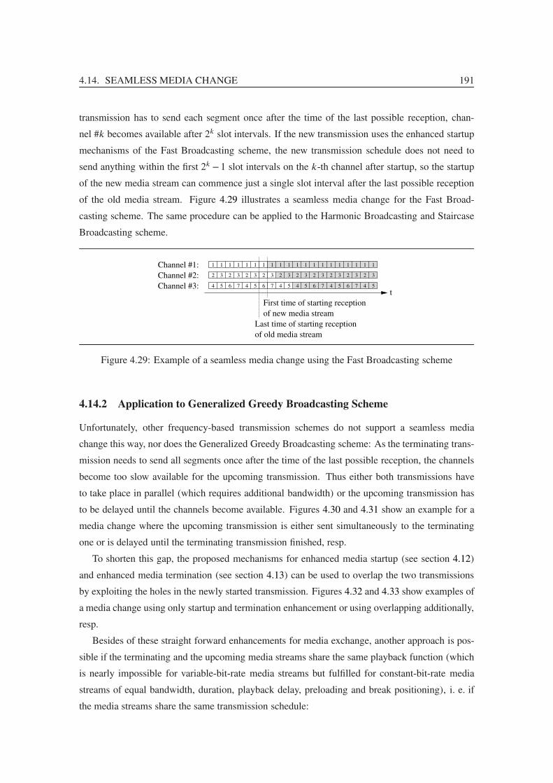
4.14. SEAMLESS MEDIA CHANGE 191
transmission has to send each segment once after the time of the last possible reception, chan-
nel #k becomes available after 2k slot intervals. If the new transmission uses the enhanced startup
mechanisms of the Fast Broadcasting scheme, the new transmission schedule does not need to
send anything within the first 2k −1 slot intervals on the k-th channel after startup, so the startup
of the new media stream can commence just a single slot interval after the last possible reception
of the old media stream. Figure 4.29 illustrates a seamless media change for the Fast Broad-
casting scheme. The same procedure can be applied to the Harmonic Broadcasting and Staircase
Broadcasting scheme.
Last time of starting reception
t
1 1 1 1
Channel #2:
Channel #3:
1 1 1 1 1 11 1 1 1 1 1 1 11 1
2 2 2 2 2 2 2 2 23 3 23 3 3 3
4 5 6 7 4 5 6 7
Channel #1:
3 3 3 3
4 5 4 5 6 7 4 5 6 7 54
of new media stream
of old media stream
First time of starting reception
Figure 4.29: Example of a seamless media change using the Fast Broadcasting scheme
4.14.2 Application to Generalized Greedy Broadcasting Scheme
Unfortunately, other frequency-based transmission schemes do not support a seamless media
change this way, nor does the Generalized Greedy Broadcasting scheme: As the terminating trans-
mission needs to send all segments once after the time of the last possible reception, the channels
become too slow available for the upcoming transmission. Thus either both transmissions have
to take place in parallel (which requires additional bandwidth) or the upcoming transmission has
to be delayed until the channels become available. Figures 4.30 and 4.31 show an example for a
media change where the upcoming transmission is either sent simultaneously to the terminating
one or is delayed until the terminating transmission finished, resp.
To shorten this gap, the proposed mechanisms for enhanced media startup (see section 4.12)
and enhanced media termination (see section 4.13) can be used to overlap the two transmissions
by exploiting the holes in the newly started transmission. Figures 4.32 and 4.33 show examples of
a media change using only startup and termination enhancement or using overlapping additionally,
resp.
Besides of these straight forward enhancements for media exchange, another approach is pos-
sible if the terminating and the upcoming media streams share the same playback function (which
is nearly impossible for variable-bit-rate media streams but fulfilled for constant-bit-rate media
streams of equal bandwidth, duration, playback delay, preloading and break positioning), i. e. if
the media streams share the same transmission schedule:

192 CHAPTER 4. GENERALIZED GREEDY BROADCASTING SCHEME
Last time of starting reception
t
of old media stream
1 1 1 1 1 1 1
2
8
4
3
2
9
5
6
2
3
4
7
2
8 3
5
6
1 1 1 1 1 1 1 11 1
4 2
3
2 2
3
2
8 3
2 2
3
of new media stream
4−
9 −
1
7
1
3
5 4 5 4 5
6 8 7 9 6 7 9
1
2
Channel #3:
Channel #2:
Channel #1:
Channel #3:
Channel #2:
Channel #1:
First time of starting reception
Figure 4.30: Example of a media change for the Generalized Greedy Broadcasting scheme where
the terminating and the upcoming media streams are transmitted simultaneously
First time of starting reception
Last time of starting reception
t
1 1 1 1 1
4 2
3
2 2
3
1 1
3
5 4 5
6 8 7 9 6
1
2
of old media stream
Channel #2:
Channel #3:
Channel #1:
of new media stream
1 1 1 1 1 1 1
2
8
4
3
2
9
5
6
2
3
4
7
2
8 3
5
6
4−
9 − 7
Figure 4.31: Example of a media change for the Generalized Greedy Broadcasting scheme where
the upcoming media stream is delayed until the terminating media stream has released the channels
Last time of starting reception
t
of old media stream
1 1 1 1 1 1 1
2
8
4
3
2
9
5
6
2
3
4
7
2
8 3
5
6
1 1 1 1 1 1 1 11 11
of new media stream
9
1 1
4
7
2 4 2 5 2 4 2 5 2 4 2 5
3 9 6 3 7 8 3 9 6 3 7Channel #3:
Channel #3:
Channel #2:
Channel #1:
Channel #2:
Channel #1:
First time of starting reception
Figure 4.32: Example of a seamless media change for the Generalized Greedy Broadcasting
scheme using enhanced startup and termination
If the schedule is not changed, it is possible to just replace the slot content in the old transmis-
sion with the new content as soon as it is not needed by any ongoing transmission, i. e. if it has
been transmitted once after the last time for a reception of the old media stream. But as segment #i
is used by the old schedule for at most πi slot intervals after the last time for a reception of the
old media stream, it is not possible for the new schedule to transmit segment #i within the first
πi slot intervals. As this is similar a requirement of live streaming (see requirement R1 in sec-

4.15. CHANGE OF MEDIA BIT RATE 193
Last time of starting reception
t
1 1 1 1
Channel #2:
Channel #3:
1 1 1 1 11 1 1 1 1 1 1 11 1Channel #1:
of old media stream
2
8
4
3
2
9
5
6
2
3
4
7
2
8 3
7
5 4
9
of new media stream
2
6
4
3
2
9
5
6
2
3
4
7
2
8
5
3
2
9
4
6
2
3
First time of starting reception
Figure 4.33: Example of an overlapping seamless media change for the Generalized Greedy
Broadcasting scheme exploiting savings from startup and termination enhancement by overlap-
ping the transmissions
tion 4.17), this problem can be solved by adding a single transmission of the whole media stream
on a separate channel. Figure 4.34 presents an example for a seamless media change using this
algorithm.
First time of starting reception
t
1 1 1 1 1 1 1 1 11 1
2
8
4
3
2
9
5
6
2
3
4
7
2
8 3
5
9 3 3 3 3
2
6 7 8 9 6 7 8
4 2 5 2 4 2 5 2 4 2 5
1
1 1 11 1 1 1 11
2 3 4 5 6 7 8 9
of new media stream
of old media stream =
Temporary Ch.:
Channel #1:
Channel #2:
Channel #3:
Last time of starting reception
Figure 4.34: Example of an enhanced seamless media change for the Generalized Greedy Broad-
casting scheme using temporarily an additional channel
4.15 Change of Media Bit Rate for Ongoing Transmissions
Instead of only starting and terminating a media-on-demand transmission, it is often desired to
modify an ongoing transmission. These modifications can be necessary when the media content
has to be updated (e. g. for a news transmission) or if the provider wants to change some parame-
ters of the transmission (e. g. to reduce the bandwidth or reduce the playback delay, depending on
the current request statistics or to adapt to expected intra-day request variations). Some of these
changes are discussed in this and the following sections.
4.15.1 Intention and Effects
A similar problem as for media replacements occurs if the bit rate of a media stream is changed:
Ongoing transmissions must not be disturbed while new transmissions should benefit from the

194 CHAPTER 4. GENERALIZED GREEDY BROADCASTING SCHEME
new media bit rate. But as the media content is identifical, some special cases can be examined to
improve the performance.
When the media bit rate is changed, several cases can be distinguished how ongoing transmis-
sions should act:
• Ongoing transmissions should be continued with the old media stream; only future requests
are served using the new media bit rate:
One solution for this case is simple but requires additional bandwidth for the time of transi-
tion: As the current transmission should continue, it has to be terminated orderly (transmit-
ting all segments which are needed to allow a proper playback for ongoing transmissions,
see section 4.13) while the new media stream transmission is started at the same time. This
means that two transmissions of the same media stream (with different bit rates) take place
at the same time until the first transmission is finished. As no receiver of one of these trans-
missions can benefit from the other transmission, this change is identical to a media content
change (see section 4.14).
If the transmission schedule can be kept (e. g. if a constant-bit-rate media stream is sent or
if the bit rate change has been foreseen when the schedule has been created), the transition
can be performed in the same way as it has been proposed for media content change with
identical transmission schedule. In this case the bit rate of the channels has to be set to
the maximum of the former and later channel bit rate during transition and one additional
channel of the target media bit rate is temporarily needed.
• Ongoing transmissions can be continued with the old or the new media stream, changing
back and forth at each segment boundary:
If segments can be played independently of each other and corresponding segments of both
media streams contain the same content (e. g. if segment boundaries are aligned to group-
of-pictures and if each segment from either transmission contains the same frames or group-
of-pictures) the change can simply be performed at the next segment boundary: The trans-
mission schedule is simply continued but the segments are replaced with the new ones and
the bandwidth of the channels is adjusted according to the new schedule. Ongoing trans-
missions will play segments of the old bit rate if these segments have been received earlier
and segments of the new bit rate if they are received after the change.
This is another case where no bandwidth is wasted, but difficult to achieve for compressed
media streams because of the fixed assignment of frames or group-of-pictures to segments.
• Ongoing transmissions can be continued with the old media stream or the new media stream,
but only a single point of change from the old to the new media stream is allowed:
4.15. CHANGE OF MEDIA BIT RATE 195
This variant poses a huge problem: As a change back to the old media stream is not allowed,
each ongoing transmission would have to play the new media stream after some time. This
means, switching to the new bit rate causes expiry of all segments which have been received
earlier for the time after the change. Thus to assure a continuous playback, the receiver
system must be able to get all these segments again in due time.
If switching to the new bit rate is scheduled with a fixed delay after start of the new trans-
mission, all segments of the new transmission must be transmitted at least once within this
delay (at least for pure pro-active systems). Unfortunately, this means that a multiple of
the new media stream bit rate is needed during the transition time (similar to the Staggered
Broadcasting scheme), so the first solution is preferred to this one.
• Ongoing transmissions can be continued with the old media stream or the new media stream,
but changes require additional data:
For the same reasons as of the previous case, no change should be applied to ongoing trans-
missions and the first variant should be used instead.
Summarizing the above, if ongoing transmissions can change back and forth between the old
and the new media stream, it is most efficient (and most simple) to perform the change immediately
at the next segment boundary. Otherwise ongoing transmissions should continue at their current
bit rate and the bit rate change is handled like a media change.
4.15.2 Application to Generalized Greedy Broadcasting Scheme
The proposed enhancement is applicable to any frequency-based transmission scheme, including
the Generalized Greedy Broadcasting scheme.
4.15.3 Alternative Solution: Layered Media Encodings
An alternative solution is possible if layered encodings are used (see also section 5.2): In this case,
a bit rate change can be realized by adding or removing enhancement layers. Similar to the above,
this can be performed in different ways:
• If ongoing transmissions should stay at their current bit rate, enhancement layers can be
added or removed as described for media startup or termination, respectively.
• If it is acceptable that ongoing transmissions will change back and forth between a different
number of layers at each segment boundary, enhancement layers can be added or removed
at the next segment boundary.

196 CHAPTER 4. GENERALIZED GREEDY BROADCASTING SCHEME
• If a single point of change is acceptable, it is also possible to add or remove the enhancement
layers and request all ongoing transmissions to ignore the added enhancement layer or to
drop data previously received for the enhancement layer, respectively.
• Changes which require additional data should still be avoided.
As the base layer (and probably some of the enhancement layers) is shared for different bit
rates, layered encodings allow a more efficient media bit rate change if ongoing transitions should
continue at their current bit rate. The only disadvantage of layered encodings is a slightly higher
total bit rate for layered media streams compared to non-layered ones.
4.16 Change of Sender Bandwidth and Playback Delay for Ongoing
Transmissions
Another possible request for modifications of ongoing transmissions is to change the playback
delay and thereby the sender bandwidth.
The simplest solution for changing the bandwidth and the playback delay is to terminate the
current transmission properly and start a new one (with a new transmission schedule) which uti-
lizes the new bandwidth and playback delay. This solution is very inefficient as several segments
are transmitted more often than necessary.
In the following, two better solutions are proposed to reduce the overhead of the change: For
the first one, a transmission schedule is created which supports halving the playback delay as well
as doubling it again later to return to the original playback delay, for the second one, a modified
version of the startup enhancement algorithm is used.
4.16.1 Dynamic Channel Addition Algorithm
Due to its binary construction, the Fast Broadcasting Protocol supports a bandwidth change in a
simple way [YCTY+01]: To add a channel, all segments are halved and the first half of the lowest
segment of each channel is moved to the next channel, i. e. the first half of segment #1 is moved to
a new channel, the first half of segment #2 to the previous position of the first half of segment #1,
the first half of segment #4 to the previous position of the first half of segment #2, and so on.
For other broadcasting protocols, a more complex algorithm has to be used, e. g. the one which
has been proposed in [PL03]: Similar to the Fast Broadcasting channel addition algorithm, this
algorithm assumes that the worst case playback delay equals the slot interval, that a constant-
bit-rate media stream is transmitted and that one channel is added to halve the playback delay.
The basic idea behind this algorithm comes from the observation that it is possible to halve the
playback delay by halving the slot interval with only one exception: The first half of all segments

4.16. CHANGE OF SENDER BANDWIDTH AND PLAYBACK DELAY 197
which had been scheduled at their required period are transmitted too seldom when the playback
delay is halved, their utilized period in the obtained transmission schedule is one too high. For
example, if the required and the utilized period of segment #i were π+i = πi = i, the period of the
first half of this segment is πi1′ = 2 · i after halving the slot interval12, but for a continuous playback
with a halved playback delay, π+i1′ = 2 · i−1 is required. The authors of the aforementioned article
solved this problem by moving these segments: The first of these segments (i. e. segment #11) is
moved to the added channel, the second one to the position of the first segment (which provides at
least a period two smaller than the old position and therefore a period which is low enough), and
so on until all necessary segments have been moved.
The complete algorithm can be described as follows:
1. A new channel is allocated and all segments of the media stream transmission are divided
into two parts of equal size, i. e. segment #i is divided into segments #i1 and #i2.
2. All segments are examined in ascending order:
• If the utilized period of the segment is equal to the required period of the segment, the
first half of the segment has to be “shifted” to a new position: Segment #11 is moved
to the new channel (where it is transmitted with the same period as before), the next
segment is moved to the previous position of segment #11, and so on. The previous
position of the last shifted segment is left unused.
• If the utilized period of the segment is lower than the required period of the segment,
it is not modified.
3. If a segment is moved to a position where it would be sent later than in its current position
(or exactly: if it is moved to a position so it is not transmitted for one period after its last
transmission), this may interrupt the continuity of ongoing playbacks. To prevent this, three
solutions are proposed:
• Additional channels can be used where these segments are transmitted once.
• As the added channel of step 1 is only used for half of the time yet, the unused positions
in it can be used for the transmission of an additional repetition of the moved segment.
• The shifting of the segment (and consequently the shifting of all following ones) can
be delayed until the segment has been transmitted the next time or until one of the
above solutions can be applied.
The first solution is the simplest one but requires temporarily additional sender bandwidth
and increases the bandwidth requirements of the receiver systems. The second solution is
12Periods are measured in multiples of the slot interval, so the period doubles if the slot interval is halved. For
clearness, the variables which refer to values after halving are marked with a tick ′.

198 CHAPTER 4. GENERALIZED GREEDY BROADCASTING SCHEME
the most elegant one, but it cannot be used in all cases as it only allows a transmission of
one further segment every slot interval. The third proposed solution has the advantage that
it does not require additional bandwidth, but it will prolong the duration of the transition
and therefore retard the halving of the playback delay.
4. When the shifting process completed, the transmission period of segment #11 is halved, so
it is transmitted permanently on the added channel thereafter. Starting from this moment,
the transmission can be joined with halved maximum playback delay.
Figure 4.35 shows an example for a dynamic addition of one channel to halve the playback delay.
It also illustrates some of the problems described above and that the change may take some time
to complete. During this time, intermediate versions of the transmission schedule are used and the
playback delay is still unmodified. Only after the change has completed, the new playback delay
can be utilized.
It is also possible to apply the bandwidth addition algorithm several times: Each time when
one channel is added, the playback delay can be halved.
4.16.2 Dynamic Channel Releasing Algorithm
To release one channel, the algorithm is applied in reverse order: Firstly, the period of segment #11
is doubled and then all segments are moved back to their original positions in reverse order (taking
the same precautions as above when a segment is moved to a later position). When all (halved)
segments have been moved to their original positions, they can be merged with their counterparts
and the (in between unused) first channel can be released.
As the releasing process only reverses the adding process, it is obvious that channels can only
be released if they have been added previously. Therefore, if a transmission scheme is needed
where k out of n channels can be released at a later time, a transmission scheme for n−k channels
has to be created and k channels have to be added using the channel addition algorithm. If this
step is performed before the transmission of the media stream is started, no ongoing transmissions
exist which can be interrupted. Therefore, the segments can be moved in any direction by the
algorithm at this time, making step 3 of the channel adding algorithm obsolete.
4.16.3 Efficiency of Channel Adding Algorithm
The efficiency of a transmission scheme where a channel has been added is unfortunately much
lower than the efficiency of a transmission scheme which has been created for the total number
of channels: Adding k channels using the channel adding algorithm increases the bandwidth by
k times the channel bandwidth and halves the playback delay k times, i. e. the efficiency η′ can be

4.16. CHANGE OF SENDER BANDWIDTH AND PLAYBACK DELAY 199
Channel #2:
−−
Channel #3:
−
111
Added Ch.:
5
1
2 44
1
3 7
1
9 36
1
8
Time of bandwidth change
−
2
1
3
2 5
8
Channel #1:
−
2
− −
(a) Original transmission and time of bandwidth in-
crease
1 2111 11 21 11 21
12 22 15 25 12 22
13 23
− −
11 21
14 24
13 23
Channel #1:
Channel #2:
Channel #3:
Added Ch.:
Time of bandwidth change
1
2
8
−
11 21
15 25 12 22 14 24
13 23 17 27 19 29 16 26 18 28
− − − − − − − − − − −
11 21 11 2
(b) Segments are halved
1 21 21
15 25 2222
13 23
12
− − − − − −
12 12
Channel #1:
Channel #2:
Channel #3:
Added Ch.: 11 −
− 21
2414
13 23
Time of bandwidth change
1
2
8
−
21
15 22 14 24
23 17 27 19 29 16 26 18 28
11
13
25
11 − 11 − 11 − 11 − 11 −
21 21 2
(c) Segment #11 is moved to the added channel
1 21 21
15 25 2222
13 23
12 12 12 12 12 12
− − −
Channel #1:
Channel #2:
Channel #3:
Added Ch.: 11 −
12 21
13 23
14 24
Time of bandwidth change
1
2
8
−
21
15 22 14 24
23 17 27 19 29 16 26 18 28
11
13
25
11 − 11 − 11 − 11 − 11 −
21 21 2
(d) Segment #21 is moved to the previous position of
segment #11
12 21 12 21 12 21 12 21 12 21
13 22 25 13 22
11 −
12 21
14 24
− 2323
11
Channel #1:
Channel #2:
Channel #3:
Added Ch.:
Time of bandwidth change
Current end of transition
1
2
8
−
21
15 22 14 24 15
23 17 27 19 29 16 26 18 28
11
12
13
25 13
−
− − − −−11 11 11 11
(e) Segment #31 would have to be moved forward to
fill the previous position of segment #21 which would
infringe ongoing playbacks; therefore it is transmitted
once in its old position, which allows to move the next
transmission of segment #31
5 13 2
−
4
−
6
−
2
−
3
11
Current end of transition
11
1
11
4
11
−
12
1
21
4
12 21
1
12
1
21 12
1
21
4
12 21
2
13
3
22
1
2 2
8
5
−
−
21
115 322
Channel #1:
24 215 2
23
Channel #2:
17
1
27
1
19Channel #3: 29
−
26
Added Ch.:
18
1
28
2
11
Time of bandwidth change
12 2
13
1
2
1
(f) Segment #41 would have to be moved forward, too,
but here another solution is possible: It is moved to its
new position and is additionally transmitted in an un-
used slot of the added channel
5 13 2
−
4
−
Channel #1:
−
2
−
3
11
Channel #2:
11
1
11
4
11
Channel #3:
12
1
21
4
12
Added Ch.:
21
1
12
6
21 12
1
21
1
12 21
1
13
4
22
1
2 2
8
5
−
2
21
115 322
3
24 215 2
23
Time of bandwidth change
17
1
27
1
19 −29
−
26
Current end of transition
18
1
28
2
11
1
12 2
13
1
2 6
(g) Segment #61 is moved to the previous position of
segment #41
1 12 21 12 21
13 22 13 22
11
12 21
24
2314
16
−
16
1114
14
25
23
− − − − − −
Channel #1:
Channel #2:
Channel #3:
Added Ch.:
Time of bandwidth change
End of transition
1
2
8
21
15 22 24 15
23 17 27 19 29 26 18 28
11
12
13
25 13
11 11 11 11
12 21 12 21 12 2
(h) Segment #41 is moved to an earlier unused position
on the added channel
1 12 21 12 21
13 22 13 22
11
12 21
24
2314
16
−
16
1114
14
25
23
11 11 11 11 11 11
Channel #1:
Channel #2:
Channel #3:
Added Ch.:
Time of bandwidth change
End of transition
1
2
8
21
15 22 24 15
23 17 27 19 29 26 18 28
11
12
13
25 13
11 11 11 11
12 21 12 21 12 2
(i) The transmission frequency of segment #11 is dou-
bled after the transition has finished
Figure 4.35: Example showing the functioning of the dynamic channel addition algorithm

200 CHAPTER 4. GENERALIZED GREEDY BROADCASTING SCHEME
calculated from the efficiency of the original transmission schedule η by
η′ = η ·Ψ0
(d+W + ·2−k
δ
)−Ψ0
(W + ·2−k
δ
)Ψ0
(d+W +
δ
)−Ψ0
(W +
δ
)+k
≈ η ·ln(
1+ d
W +·2−k)
ln(
1+ d
W +
)+k
(4.25)
Table 4.4 shows the efficiency for different playback delays. This table shows that the efficiency
of the transmission schedule is lowered by a factor of approximately 0.903 if the playback delay is
halved from ten to five minutes this way. On the other hand, the efficiency stays nearly unchanged
if the playback delay is very short (e. g. near to the slot interval).
Original New Efficiency quotient
playback delay playback delayη′η
10 min 5 min 0.903
5 min 2.5 min 0.923
2 min 1 min 0.939
1 min 30 s 0.948
20 s 10 s 0.959
10 s 5 s 0.967
6 s 3 s 0.973
4 s 2 s 0.981
2 s 1 s 0.999985
Table 4.4: Efficiency effects of dynamic channel addition algorithm for adding one channel to a
two hour media stream with one second slot intervals
4.16.4 Application to Generalized Greedy Broadcasting Scheme
To apply this algorithm to the Generalized Greedy Broadcasting scheme, it has to be generalized as
the Generalized Greedy Broadcasting scheme allows to increase the playback delay independently
of the segment size (see section 4.5) and even allows to create transmission schemes which adapt
to a given playback function of a media stream (see sections 4.7 and 4.8). The effects of these
generalizations to the bandwidth changing algorithms are proposed in this section in several steps:
Firstly, the mechanisms of the above algorithm are described separately and are generalized. This
is necessary as they are actually independent from each other and are not needed all at the same
time in every setup. In a second step, one special case is examined: Transmission schemes which
have a linear playback function (i. e. for a constant-bit-rate media stream with playback delay and
partial preloading, but no other extensions). In a third step, proposals for improvements are given,
e. g. ways to reduce the transition time from one schedule to another.
The algorithm which has been proposed above is comprised out of several mechanisms:
• Preparing to change the playback delay:
4.16. CHANGE OF SENDER BANDWIDTH AND PLAYBACK DELAY 201
This step seems to be the most simply one: The playback delay is changed internally to the
desired value. But as the transition to the new schedule may take some time, the receiver
systems must not use the new playback delay until the transition completed.
The algorithm proposed in [PL03] only examined the process of halving the playback delay
by adding one channel. This can be generalized: In the following, any reduction of the
playback delay is examined. The additionally needed bandwidth in this case may be higher
or lower than one channel and is also influenced by some other conditions (e. g. the amount
of preloading or the playback function in case of variable-bit-rate media streams).
• Splitting segments and the slot interval:
In the algorithm proposed in [PL03], all segments are halved in this step. This was necessary
as the playback delay is equal to the slot interval in the supported transmission schemes of
the described algorithm and the playback delay was to be halved.
For the generalized case, any type of splitting is to be examined: A split into more than one
subsegment may be interesting if the playback delay is reduced to a value shorter than half of
the slot interval or if the desired playback delay cannot be reached accurately enough using
the halved playback delay (i. e. if it is not close to a multiple of the halved slot interval).
Instead of splitting segments into two or even more parts, it may be unnecessary to perform
any splitting in other cases. For example, if the desired playback delay can be expressed as
a multiple of the slot interval or if the segment size is already as small as practically possible
or desired (as described in section 4.5, some bandwidth can be saved if segments are made
as small as possible), further splitting is actually unnecessary or impossible.
Strictly speaking, the bandwidth savings by splitting are the same that are gained by de-
coupling the playback delay and the slot interval (see section 4.5). As described there, the
bandwidth requirements can be reduced by using as small segments as possible (always
keeping the overhead in mind which is necessary at the receiver to identify the segments as
well as the storage seek overhead which grows if the segments become smaller). Therefore,
if the results of decoupling the playback delay have been considered when the transmission
scheme has been generated, further splitting is neither required nor advisable.
• Moving segments:
To allow a continuous playback with the new playback delay, some segments have to be
moved to a position with a lower period. In the algorithm proposed in [PL03], the first half
of all segments which had been scheduled to a position where their utilized period equals
the required period had to be moved. The algorithm moved the first segment to the added
channel and moved the latter segments to the released positions of the preceding moved
segments. This way a queue of segments is build which are shifted by one position.

202 CHAPTER 4. GENERALIZED GREEDY BROADCASTING SCHEME
In the generalized case, it may be necessary to move more segments than described above
and to move the segments in the queue by more than one position: For the most generalized
case, a playback function describes the playback time for any part of the media stream
(see section 4.1.2), and equation (4.22) defines how the required segment period can be
calculated from a cumulative bandwidth function. As the cumulative bandwidth function
includes the playback delay, a change of the playback delay results in a new cumulative
bandwidth function f ′ and a new sequence of required segment periods (π+i′)i∈{1,...,n}. Using
this sequence of required periods and the sequence of utilized periods of the old schedule, it
is possible to calculate the number of positions k by which the segments have to be shifted
in the queue using the following equation:
k = min{j ∈ {1, . . . ,n} | ∀i ∈ {j+1, . . . ,n} : π
+i′ ≥ πi−j
}(4.26)
The bandwidth which is additionally required in this moving process is equal to the band-
width of the first k segment transmissions. To schedule these segments efficiently, the Gen-
eralized Greedy Broadcasting algorithm can be used again.
• Utilizing the changed playback delay:
After the transition completed, the new playback delay can be used by the recipients.
4.16.5 Simplified Application for Basic Transmissions
As a special case, a transmission scheme which uses increased playback delay and partial preload-
ing but no other of the previously described extensions is examined below. These schemes have
two benefits: They are very simple (e. g. in contrary to variable-bit-rate transmission schemes
where the required periods of the segments depend on the playback function of the media stream)
and very popular (because constant-bit-rate media streams are still very common).
Additionally, it is assumed that the schedule already uses the smallest utilizable segment size
to save the bandwidth which is gained by this procedure (see section 4.5) so the splitting step for
segments can be skipped. (Otherwise splitting can simply be performed beforehand and indepen-
dently of the playback delay and bandwidth modification.)
If an increased playback delay and/or partial preloading is used for a constant-bit-rate media
stream, the required period of segment #i can be calculated by π+i = i− 1+
⌊W ++f−1(P )
δ
⌋(see
equation (4.17)). Similarly, to allow a continuous playback using a new playback delay W +′,
the period of segment #i must be less or equal to π+i′ = i− 1+
⌊W + ′+f−1(P )
δ
⌋. According to this,
all segments #i with πi > π+i′ have to be moved. In case of a perfect schedule, where πi = π
+i is
fulfilled for all segments #i (which is impracticable, see section 3.7.1), this means that all segments

4.16. CHANGE OF SENDER BANDWIDTH AND PLAYBACK DELAY 203
would have to be moved by
k = min{j ∈ {1, . . . ,n} | ∀i ∈ {j+1, . . . ,n} : π+i′ ≥ πi−j}
= min{j ∈ {1, . . . ,n} | ∀i ∈ {j+1, . . . ,n} : π+i′ ≥ π
+i−j}
= min{j ∈ {1, . . . ,n} | ∀i ∈ {j+1, . . . ,n} :
i−1+⌊W + ′+f−1(P )
δ
⌋≥ i− j−1+
⌊W ++f−1(P )
δ
⌋}
= min{j ∈ {1, . . . ,n} |⌊W + ′+f−1(P )
δ
⌋≥⌊W ++f−1(P )
δ
⌋− j}
=⌊W ++f−1 (P )
δ
⌋−⌊W + ′+f−1(P )
δ
⌋(4.27)
positions.
In a realistic transmission schedule, πi is very near but often smaller than π+i , so only few
segments have to be moved if k is very small. On the other side, if k is huge (i. e. if the playback
delay is reduced considerably), most segments have to be moved.
Figure 4.36 illustrates this in an example where one channel is added to a transmission schedule
which has a maximum playback delay of twelve slot intervals: Adding one channel allows to halve
the maximum playback delay, so the period of all segments must be reduced by six in the resulting
schedule. As no segment has been scheduled with a period six higher than needed, all segments
have to be moved in this example.
At first glance, this generalization seems to be much worse than the algorithm proposed by the
authors of [PL03] where only few segments had to be moved by k = 1 positions in the queue. The
reason for this is hidden in the slot interval: The original algorithm is based on the fact that the slot
interval is as long as the (worst case) playback delay while the above proposed algorithm allows
to use a playback delay of several slot intervals. In other words: The original algorithm benefited
from the fact that the schedule was indeed very inefficient compared to the schedule using the
short slot interval.
This insight can be used to lower the number of segments which have to be moved: If seg-
ments are intentionally scheduled in such a way that their utilized period is k lower than their
required period, these segments are not involved in the moving process. The bandwidth loss can
be controlled much more precisely than by using a longer slot interval: As the first segments need
the most bandwidth, they can be scheduled as good as possible, while only the latter segments
are excluded from the moving process by lowering their period requirements artificially for the
scheduling process. If several bandwidth changes are intended, it is possible to adjust the periods
for the shortest of the playback delays. Alternatively, it is even possible to reduce the period of
different numbers of segments for each planned playback delay.
The efficiency loss by decreasing the period of the latter part of a media stream is exactly
the same as the efficiency gain that has been described for the insertion of breaks into a stream

204 CHAPTER 4. GENERALIZED GREEDY BROADCASTING SCHEME
Channel #1
2 3 4 9876
16151413
12111051
(a) Original transmission schedule before bandwidth change
Added Channel
151413121110987
3654
21−
−
−−−−
−−
Channel #1
16
(b) Resulting transmission schedule after halving the playback delay
Figure 4.36: Example of a dynamic bandwidth change for a transmission scheme using a playback
delay of twelve slot intervals
transmission. This is evident as decreasing the period of the latter part equals to moving this part
to an earlier position in the playback, thus it can be contemplated as a negative break.
Figure 4.37 illustrates this in a similar setup as of the previous example: The original maximum
playback delay is twelve slot intervals and it should be halved by adding a channel. In contrast to
the previous example, segments #8 and higher have been scheduled with a period six lower than
necessary. (Therefore, only fourteen instead of sixteen segments fit into the schedule.) When the
playback delay is halved in this case, only the first seven segments have to be moved.
4.16.6 Alternative Solution: Transition between different Transmission Schedules
Instead of adding one channel and moving segments in a queue-like fashion to transit from the old
schedule to the new one, another solution is presented in this subsection. This approach is based
on the simple idea to transmit data for two different transmission schemes (one utilizing the old
playback delay and one for the new playback delay) in parallel, using the enhanced termination
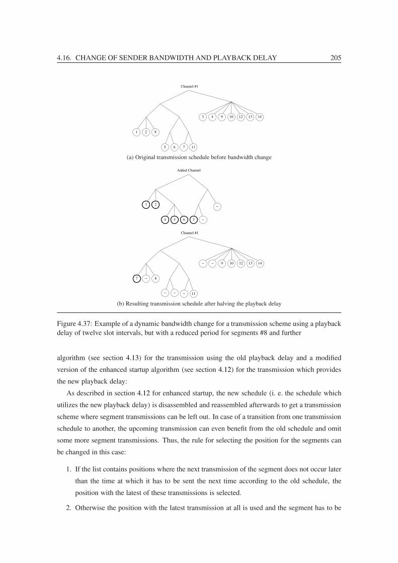
4.16. CHANGE OF SENDER BANDWIDTH AND PLAYBACK DELAY 205
Channel #1
134 9 103 12
11765
1 2 8
14
(a) Original transmission schedule before bandwidth change
Added Channel
7
3654
21
−
− − −
− −
−
−
14139 10 12
11
Channel #1
8
(b) Resulting transmission schedule after halving the playback delay
Figure 4.37: Example of a dynamic bandwidth change for a transmission scheme using a playback
delay of twelve slot intervals, but with a reduced period for segments #8 and further
algorithm (see section 4.13) for the transmission using the old playback delay and a modified
version of the enhanced startup algorithm (see section 4.12) for the transmission which provides
the new playback delay:
As described in section 4.12 for enhanced startup, the new schedule (i. e. the schedule which
utilizes the new playback delay) is disassembled and reassembled afterwards to get a transmission
scheme where segment transmissions can be left out. In case of a transition from one transmission
schedule to another, the upcoming transmission can even benefit from the old schedule and omit
some more segment transmissions. Thus, the rule for selecting the position for the segments can
be changed in this case:
1. If the list contains positions where the next transmission of the segment does not occur later
than the time at which it has to be sent the next time according to the old schedule, the
position with the latest of these transmissions is selected.
2. Otherwise the position with the latest transmission at all is used and the segment has to be

206 CHAPTER 4. GENERALIZED GREEDY BROADCASTING SCHEME
transmitted once additionally not later than the time at which the segment has to be sent
according to the old schedule.
Similar to the enhanced startup, the results can be improved by using two rounds for the reassem-
bly.
Figure 4.38 shows examples of a playback delay change of a media stream with eight segments,
from six slot intervals to two intervals and vice versa. For the change from six to two intervals, a
transition from a one-channel transmission to a two-channel transmission is performed, and due
to the modified enhanced startup, the old transmission can be terminated immediately. For the
reverse direction, two segments have to be transmitted once before the old transmission can be
terminated.
1 3 1
t761 2 3 54 8
761 2 3 54 8
761 2 3 54 8Recipient #3:
Recipient #2:
Recipient #1:
1 1 13 2 5 7 4 6 2 3 8 5 4 2 6 7 3 − − −− 8
4
5 8 2
4 1 3 1
8 27 6 2
1 3 1
7 6 2
4
5 5
4
New channel #2:
New channel #1:
Old channel #1:
(a) Transition from a schedule with a playback delay of six slot intervals to a schedule with two slot intervals
5 5
t
Recipient #2:
Recipient #3:
Recipient #1:
Old channel #1:
Old channel #2:
New channel #1:
4
5 8 2
4 1 3 1
8 27 6 2
1 3
7 6
4
5 5
1 3 1
1 3 2 8 6 1 2 3 7 1 3 2
−
8
− −
−
1 2 3 4 5 6 7 8
761 2 3 54 8
761 2 3 54 8
4
(b) Transition from a schedule with a playback delay of two slot intervals to a schedule with six slot intervals
Figure 4.38: Examples of a bandwidth change using enhanced transitions between two schedules
4.16.7 Comparison
Both of these procedures, the channel adding algorithm and the transition between different trans-
mission schemes, have their own benefits: The advantage of the former channel adding algorithm
is that the bandwidth change can be performed without any further additional bandwidth resources.
As a disadvantage, the transitions may take a long time. During these transition times, the trans-
mission consumes the higher of the bandwidths of the two schedules without granting the lower
playback delay. Thus the schedule is very inefficient while the transition takes place (e. g. the
efficiency is lowered to about 89,88% if the halved playback delay is 17200
of the media stream
duration and about 71,95% if the halved playback delay is 112
of the media stream duration13).
13These fractions equal to a playback delay of one second and 10 minutes of a two hour media stream.

4.16. CHANGE OF SENDER BANDWIDTH AND PLAYBACK DELAY 207
Additionally, the transition to a different transmission scheme has the advantage that it is based on
more efficient transmission schedules.
To make the schemes comparable, additional channels are provided for both algorithms which
are used to transmit segments when they do not fit in the transition schedule. Providing these
additional channels, both algorithms can perform the playback delay change immediately and
their efficiency can be measured by examining the amount of additionally transmitted segments
and the efficiency of the used schedules. For the comparison, a constant-bit-rate media stream of
7 200 segments is assumed.
Table 4.5 shows the fraction of the media stream which has to be transmitted on additional
channels by the two algorithms when performing a change from one playback delay to another.
This fraction varies between 35.47 % and 64.63 % in this example when the playback delay is
changed using the segment shifting algorithm and between 3.47 % and 28.17 % when the media
transition algorithm is used.
In addition to the amount of additionally needed bandwidth during transition, the efficiency of
schedule after changing the playback delay is also important because it has long-term effects on
the needed bandwidth. Table 4.6 shows the efficiency of the resulting transmission schemes after
reducing the playback delay from 900 slot intervals to value between 1 and 240 slot intervals for
both algorithms. While the efficiency of the schedules of the segment shifting algorithm drops to
values below 80 % when performing significant changes of the playback delay, the efficiency for
the media transition algorithm stays always above 99 %.
Due to these results, the media transition algorithm should be preferred in any case as it needs
to transmit much less segments on the additional channel (in some cases about only one tenth of
the amount of the shifting algorithm) and grants a much better transmission schedules at the same
time.
As described earlier, the number of segments which have to be moved by the shifting algorithm
can be reduced by decreasing the periods artificially. But besides lowering the number of segments
to move, this reduces the efficiency of the transmission schedules further, so the gap between the
two algorithms cannot be closed this way. (Lowering the periods shows also positive effects for
the adjusting algorithm.)
This means that the adjusting algorithm should be preferred in all cases where possible (i. e.
where additional bandwidth for the time of the transition is available). The only disadvantage of
this procedure is that the receiver systems must be able to receive the additional channels, i. e.
the necessary receiver bandwidth is increased for the duration of the transition for all ongoing
receptions, too.
Another advantage of the above proposed adjusting transmission schedule transition algorithm
is that this procedure allows to transit between arbitrary schedules for the same media stream:

208 CHAPTER 4. GENERALIZED GREEDY BROADCASTING SCHEME
New Old Playback Delay (in slot intervals)
Playback
Delay 1 4 15 60 240 900
1 — 35.47% 45.60% 46.19% 43.32% 36.33%
4 64.51% — 44.68% 46.22% 42.38% 35.29%
15 54.13% 55.24% — 44.08% 46.18% 35.53%
60 53.75% 52.82% 55.69% — 44.56% 35.94%
240 56.65% 57.57% 53.56% 54.58% — 39.85%
900 63.63% 64.63% 64.46% 63.96% 60.11% —
(a) Amount of a 7 200 segment media stream which has to be transmitted on additional channels when the playback
delay is changed using the shifting algorithm
New Old Playback Delay (in slot intervals)
Playback
Delay 1 4 15 60 240 900
1 — 10.08% 9.01% 8.31% 4.81% 3.47%
4 8.13% — 9.01% 7.14% 4.31% 3.69%
15 9.06% 11.44% — 9.65% 5.40% 3.58%
60 10.81% 12.42% 11.44% — 5.85% 4.50%
240 14.46% 16.19% 15.14% 14.17% — 5.56%
900 26.89% 28.17% 26.58% 26.83% 21.01% —
(b) Amount of a 7 200 segment media stream which has to be transmitted on additional channels when the playback
delay is changed using the adjusting algorithm
Table 4.5: Comparison of the two proposed algorithms for changing the bandwidth of an ongoing
transmission
Playback Delay 1 4 15 60 240 900
Efficiency 79.85% 77.46% 77.96% 80.46% 86.00% 99.63%
(a) Efficiency of transmission schemes which are gained by shifting algorithm, starting with the transmission scheme
for a playback delay of 900 slot intervals
Playback Delay 1 4 15 60 240 900
Efficiency 99.66% 99.54% 99.48% 99.27% 99.52% 99.63%
(b) Efficiency of transmission schemes which are gained by adjusting algorithm, starting with the transmission scheme
for a playback delay of 900 slot intervals
Table 4.6: Comparison of the efficiency of the transmission schemes used by the two proposed
algorithms
Besides of using the algorithm for changing the playback delay, it is also possible to insert, remove
or modify breaks in the transmission or to change the amount of preloading.

4.17. LIVE TRANSMISSIONS 209
4.17 Live Transmissions
Live streaming means the ability to capture a media stream and transmit it immediately after
capturing. This imposes additional requirements to the transmission scheme as no data can be
transmitted in advance, i. e. before it has been captured.
Unfortunately, nearly all of the broadcasting schemes assume that the media stream is com-
pletely available at the beginning of the transmission, thus most of them cannot be used for live
transmissions originally.
4.17.1 Intention and Effects
In order to modify transmission schemes for live transmission support, it is important to exam-
ine the characteristics of a broadcasting scheme which supports live streaming. The authors
of [YCTY+01, YYT03] summarized these characteristics in form of three requirements, but as
one of these requirements (the transfer rate for the segments must not be higher than the media
production rate) cannot be applied to variable-bit-rate media streams, a modified version of these
requirements is presented here:
R1. The transmission schedule must not demand to broadcast media data before it has been
captured.
If a transmission schedule requires transmitting data which has not yet been captured, it
cannot be sent at this moment. Delaying the transmission until it has been captured may
exceed the available bandwidth and sending it at its next planned transmission time may be
too late for a continuous playback at the receiver system.
R2. The transmission scheme must tolerate the varying length of the live program.
As the available bandwidth is limited in most cases, the transmission schedule cannot re-
quest more bandwidth if the media becomes longer than expected. Instead, other parameters
(e. g. playback delay) should be changed in this case.
The first requirement is satisfied only by Harmonic Broadcasting, Staircase Broadcasting and
Fast Broadcasting (with minor changes as shown in [YCTY+01]), but by increasing the bandwidth
temporarily (for the duration of one transmission of the media stream) for one additional trans-
mission of the live media stream as described in [YYT03], it is possible to fulfill this requirement
for any frequency-based transmission scheme, too.
Figure 4.39 shows an example of a frequency-based transmission where an additional live chan-
nel has been added. In this figure, segments which cannot be transmitted in the original schedule
(as they have not yet been captured) have been marked with a cross and segment transmissions
which can be omitted (because they have already been sent on the live channel) have been marked
with a slash.

210 CHAPTER 4. GENERALIZED GREEDY BROADCASTING SCHEME
Channel #1:
Channel #2:
Channel #3:
Channel #4:
Live Channel: 762 3 54 158 9 1110 1312 1716 18 19 20
1
4
3 6
5 10 12
9
8 16 17
7 18 22 19 23
14 15
1
2
14
1
14
1
1 1 1 1 1 1 1 1 11 1 1 1 1 1 11
5 105
t12 525
2 2 4 2 2 4 82 2 4 2 2 4 82
3 3 6 3 97 3 6 3 7 3 6
1311 20 24 1311 21 15
Figure 4.39: Example of a live media transmission using the Greedy Broadcasting scheme and an
additional live channel
To fulfill requirement R2, it is necessary to reduce the total bandwidth requirements of an
ongoing transmission dynamically, so that the gained bandwidth can be used for a prolongation of
the transmission as necessary. This can be achieved by increasing the playback delay as described
in section 4.16. Unfortunately, this either needs additional bandwidth for the time of the transition
to the longer playback delay or takes some time, thus a bandwidth change has to be considered
timely in advance.
If additional bandwidth for an extension is available, a new channel can be allocated and the
next segments scheduled onto it. The transmission schedule created this way is expected to be
slightly less efficient than one which has been created initially for the increased bandwidth but
provides still the same playback delay.
Similar but not as strict requirements apply for near-live streaming, where a short delay between
capture and transmission is used. This delay increases the number of duplicate segments of the live
channel and the ordinary transmission schedule and therefore can be used to lower the additionally
needed bandwidth slightly.
4.17.2 Application to Generalized Greedy Broadcasting Scheme
Using a live channel to fulfill requirement R1 can also be used for the general case in conjunction
with the Generalized Greedy Broadcasting scheme with the following constrictions:
• Similar to above, the media stream duration is not always known in advance. Therefore, the
transmission schedule may use too much channels if the duration is overestimated and may
be less efficient if an additional channel is added in case of an underestimation.
• If the cumulative bandwidth function is not known in advance (e. g. if the media stream
uses a variable-bit-rate encoding or if the location of breaks is not known in advance), the
schedule cannot be generated in advance at all. Instead, each segment has to be added in
real-time into the transmission schedule using the Generalized Greedy Broadcasting sched-
uler algorithm. This means that it is not possible to try different weights in the Generalized
Greedy Broadcasting scheduler algorithm to improve the efficiency of the schedule. An-
other consequence is that it is not possible to calculate the needed bandwidth for a given

4.17. LIVE TRANSMISSIONS 211
media stream duration in advance as the bandwidth depends on the cumulative bandwidth
functions.
• In case of a variable-bit-rate media stream, the live channel must be able to transmit the
variable-bit-rate media stream. Due to the live constraint, no smoothing is possible to elim-
inate bandwidth peaks.
To reduce the impacts of these problems, the following enhancements can be used:
• When the live transmission ends (i. e. the media stream is completely available at the sender
system), it is possible to create a better transmission schedule and migrate to this one us-
ing the transition algorithm for different playback delays which has been presented in sec-
tion 4.16.6. This may be esp. beneficial if the efficiency of the transmission schedule is low
as a result of using a single weight combination for the Generalized Greedy Broadcasting
schedule algorithm when generating a schedule for variable-bit-rate live media streams.
• To reduce the number of segments which have to be transmitted additionally due to the live
channel transmission, another modified version of the startup enhancement algorithm (see
section 4.12) can be used. The rule for selecting the best node N for a segment #i from the
list of all possible nodes N is changed as follows:
LetP ={N ∈N
∣∣ΦN +2 ·ΠN < 2 ·π+i
}be the list of segment positions so that segment #i
can be placed in such a way that its first two transmissions can be omitted.
1. If P �= ∅, select (one of) the node(s) of this set which provides the latest segment
transmission, i. e. N ∈ argmaxM∈P
(ΦM +2 ·ΠM ).
2. If P = ∅, select the node with the latest segment transmission of all possible nodes,
i. e. N ∈ argmaxM∈N
(ΦM +2 ·ΠM ).
These rules are similarly designed as the ones in section 4.12 with the exception that they
exploit the segment transmission on the live channel: As each segment is transmitted on the
live channel at its latest possible time (i. e. at t = δ ·π+i ), the next segment transmission is
not needed before 2 · δ ·π+i . This allows to omit the first segment transmission in all cases
and the second one if it occurs before slot 2 ·π+i (which is the case if the first of the above
two rules applies).
• If a near-live transmission is sufficient (i. e. a delay between capturing and transmission can
be accepted), a limited smoothing is possible which reduces the bandwidth peaks of the live
channel a bit.
Summarizing the above, the Generalized Greedy Broadcasting scheme allows live transmis-
sions if an additional live channel is temporarily added. Problems like an unknown media stream

212 CHAPTER 4. GENERALIZED GREEDY BROADCASTING SCHEME
duration, a minor efficiency loss when generating the schedule at real-time, the additional amount
of bandwidth for the live channel and the varying of the bandwidth of the live channel can be
solved very efficiently with the Generalized Greedy Broadcasting scheme.
4.18 Support for Receiver Systems with Limited Bandwidth
Most of the proposed segmenting transmission schemes benefit from the fact that segment trans-
missions can be received by several receiver systems if the systems are already listening to the
transmission. But this requires that all receiver systems are able to receive many segments at once
and that they are able to store them temporarily. As this causes high bandwidth and storage re-
quirements for the receiver systems, it is important to examine these requirements and search for
alternative solutions. In the following of this section, the bandwidth requirements are examined
and, in the next section, an inspection of the storage requirements is given.
4.18.1 Intention and Effects
For most of the presented transmission schemes (and nearly all of the frequency-based schemes),
the receiver systems must be able to receive all data which is sent by the sender system, i. e.
the receive bandwidth requirements of the receiver systems are equal to the send bandwidth re-
quirements of a sender system for one media stream. But as all segments must only be received
once, the bandwidth requirements of the receiver system decrease throughout the transmission.
Figure 4.40 shows how long the channels of a transmission have to be joined by two recipients
which joined the reception at different times and thus the bandwidth requirements of the two re-
cipients. Because of the different join times, the bandwidth requirements of the two recipients
differ slightly. Figure 4.41 shows this for a more simple example for two receivers: The maxi-
mum bandwidth requirements for recipient #1 is three times the media bit rate while recipient #2
only has to receive data of twice the media bit rate, and the bandwidth requirements differ mainly
during the transmission for these recipients.
If the bandwidth of the receiver system does not allow a reception of all channels of a media
transmission at once, the sender system can accommodate the transmission schedule to allow a
media reception by these recipients:
The basic idea here is that the receiver system uses a sliding window for the channels it receives:
If the receiver system can only receive R out of N channels at once, it first receives the first R
channels. When the first of these channels is not needed any more, it is dropped and the next
channel is joined. This is continued until all channels have been joined. In other words, the
receiver system first receives channels #1, . . . ,#R, then #2, . . . ,#(R+1), and so on, until finally the
channels #(N −R+1), . . . ,#N are received.

4.18. RECEIVER SYSTEMS WITH LIMITED BANDWIDTH 213
0
1
2
3
4
5
0 1000 2000 3000 4000 5000 6000 7000
Ban
dw
idth
in m
ult
iple
s of
med
ia b
itra
te
Time after reception beginning
Max. bandwidth of recipient 1Max. bandwidth of recipient 2
Figure 4.40: Max. bandwidth requirements of two recipients of a Generalized Greedy Broadcast-
ing scheme transmission with 7 200 segments and a playback delay of 60 slot intervals
of recipient #2:
Recipient #1:
Bandwidth req.
Channel #3:
of recipient #1:
Channel #2:
Recipient #2:
Channel #1:
Bandwidth req.
1
987654321
1 1 1 1 1 1 1 1 1 11 1 1 1 1 1 1 11 1
2 2 2 2 2 2 2 2 2 2
3 3 3 3 3 33
t98 8 9 8 9 6
545 4 5 4 5 4 5 4
66 677 7
987654
3
0
3
0
32
Figure 4.41: Max. bandwidth requirements of two recipients of a Generalized Greedy Broadcast-
ing scheme transmission
When the transmission schedule for a channel #i > R for such a system is created, one has
to consider that the channel is joined with the latency Ji by the recipients. This latency can
be calculated from the join latency Ji−R of the left channel #(i−R), the (worst case) channel
reception duration (which is equal to the maximum segment period Pi−R of this channel times the
slot interval δ) and the time which is required for leaving and joining channels J :

214 CHAPTER 4. GENERALIZED GREEDY BROADCASTING SCHEME
Ji =
⎧⎨⎩Ji−R+Pi−R · δ+J if i > R,
0 if i ≤R
=� i−1
R �∑j=1
(Pi−j·R · δ+J
)Pi = max{πj|1 ≤ j ≤ n ∧ κj = i}
(4.28)
This idea (without an extra channel leave/join latency) has been studied in [PL00] for the Fast
Broadcasting and New Pagoda Broadcasting schemes and gives good results in many cases.
4.18.2 Application to Generalized Greedy Broadcasting Scheme
This approach can be applied nearly unmodified to the Generalized Greedy Broadcasting scheme.
Similar to the procedure in [PL00], best results are achieved by this approach for the Generalized
Greedy Broadcasting scheme if the segments on the first N −R channels are scheduled on one
channel after another. That is the first segments are scheduled on the first channel, when it is full
the next channel is filled, and so on until N −R channels have been filled. The last R channels
can be filled at once.
This means that the scheduling algorithm of the Generalized Greedy Broadcasting scheme has
to be adjusted slightly:
• To fill one channel after another, the Generalized Greedy scheduler algorithm is applied to a
single channel only. When the channel is full, the Generalized Greedy scheduler algorithm is
called again for the next channel, supplying the list of remaining segments to the scheduler.
This is continued until N −R channels have been filled. For the remaining R channels, the
Generalized Greedy scheduler algorithm is called a last time and the channels are filled at
once with the remaining segments.
• When searching for a node in the transmission trees which can be used for the transmission
of a segment, the join delay of the channel has to be taken into account: To allow a continu-
ous playback at the receiver side, the join delay has to be subtracted from the playback time
when calculating the required period of the segment, i. e. the needed period of segment #i
on channel #j can be calculated by
π+i,j =
⌊F−1((i−1) ·σ)−Jj
δ
⌋(4.29)
if an inverse playback function F−1 is used and immediate segment reception is possible (see
section 4.9). Additionally, the efficiency of the resulting transmission schedule is increased
if the quality function for the search of the best fitting node for a segment takes the join

4.18. RECEIVER SYSTEMS WITH LIMITED BANDWIDTH 215
latency of the node into account:
QIi,N
=π+i,KN
modΠN
ΠN
QIIi,N
=ΠN
π+i,KN
QIIIi,N
=JKN
π+i,KN
·δ
Qi,N = (1−W II −W III ) ·QIi,N +W II ·QII
i,N +W III ·QIIIi,N
(4.30)
But when this approach is applied to the Generalized Greedy Broadcasting scheme, the results
sometimes lag behind the ones of the New Pagoda Broadcasting scheme, and in other cases they
are much behind the theoretical limit for this setup. The reason for this penalty is that the General-
ized Greedy Broadcasting scheme is too efficient: The Generalized Greedy Broadcasting scheme
manages to put more segments in the first channels than the New Pagoda Broadcasting scheme as
it uses higher segment periods. As a result, the former channels must be joined for a longer time
due to the higher periods. This increases the channel join latencies of the later channels which
thereby loose much of their efficiency.
The solution is to lower the efficiency of the Generalized Greedy Broadcasting scheme for the
first channels to improve the overall efficiency: If a segment period limit P+i is introduced for
channel #i, the duration for reception of this channel can be shortened. As the receiver is able
to receive R channels at once, this limit is only needed for the first N −R channels, for the last
R channels no limit is required nor beneficial.
To calculate the optimal segment period limit for a channel, the remainder of this section has
to make the additional assumption that each segment can always be scheduled with its maximum
period (or the segment period limit of the channel, whichever is lower). This is normally not true
as nearly any transmission scheme schedules some segments at a lower segment period than they
require in order to fit them into the transmission schedule. As a minor compensation, the channel
bandwidth is lowered by 1 % for these calculations, which should reflect that the Generalized
Greedy Broadcasting scheme operates at an efficiency around 99 %.
Using these assumptions, the consumed bandwidth of a segment #i on channel #κi can be
calculated as max{
1
π+i
, 1
P+κi
}. As the bandwidth of each channel is limited, the following relation
has to be fulfilled at the same time:
0.99 ≥
⎧⎪⎪⎨⎪⎪⎩
xk∑i=xk−1+1
max{
1
π+i
, 1
P+k
}if k ≤N −R
xk∑i=xk−1+1
1
π+i
if k >N −R
(4.31)
where xk is the index of the last segment which can be transmitted on channel #k. (x0 is assumed
to be 0 to omit an extra case for k = 1.)
216 CHAPTER 4. GENERALIZED GREEDY BROADCASTING SCHEME
To get the best efficiency, the total number of segments n= xN has to be maximized by selecting
the optimal set of channel period limits P+i for all channels #i ≤N −R. The search for the best
set of channel period limits can be performed using a brute-force algorithm which tries different
limits and calculates n = xN using the above relation.
For example, for a constant-bit-rate media stream or 7 200 segments, a playback delay of 60 slot
intervals and a receiver bandwidth limit of twice the media bit rate, the Fixed Delay Pagoda Broad-
casting scheme needs a total bandwidth of 6.759 times the media bit rate. Without application of
period limits, the Generalized Greedy Broadcasting scheme needs 6.596 times the media bit rate
(i. e. about 2.41% less than the Fixed Delay Pagoda Broadcasting scheme) and 6.282 times the
media bit rate if the period limits 111, 302, 575, 1201 and 2716 are applied to the first five chan-
nels, respectively (about 7.05% less than the Fixed Delay Pagoda Broadcasting scheme).
4.19 Support for Receiver Systems with Limited Storage
Similar to a limitation of the receiver bandwidth, receiver systems may be short of storage for
buffering segments for later playback. This leads to two new topics which needs further exami-
nation: How much storage is required for a successful reception and playback of a media stream
for a given transmission schedule and how can the memory requirements be lowered for poorly
equipped receiver systems? In the following of this section, two algorithms for calculating the
memory requirements are proposed, followed by a mechanism to lower the storage requirements.
4.19.1 Exact Calculation of Storage Requirements for Frequency-Based Transmis-
sion Schemes
The calculation of the storage requirements for a frequency-based transmission schedule has
turned out to be very complicated: As the storage requirements depend on the exact time when the
recipient joined the transmission, the brute-force approach would demand to calculate the require-
ments for every distinguishable join time. Although it is very simple to calculate the exact storage
requirements for a given joining time (by simulating the transmission), the number of simula-
tions which have to be performed this way equals the period of the whole transmission schedule.
The period of the whole transmission schedule equals the least common multiple of all segment
periods of the transmission schedule and is very high for most transmission schedules14: For ex-
ample, the period of a transmission schedule of the Generalized Greedy Broadcasting scheme for
7 200 segments and a maximum playback delay of 60 slot intervals is about 5 ·1044.
The following algorithm circumvents this brute-force examination by splitting the transmission
schedule into independent sub-schedules: Two (or several) sub-schedules are considered to be
14The most prominent exceptions is Fast Broadcasting where the transmission schedule has a period of 2N−1.

4.19. RECEIVER SYSTEMS WITH LIMITED STORAGE 217
independent if the set of prime factors of all periods of the segments for each of the sub-schedules
are pairwise disjoint. For example, if the schedule contains the segments with periods from 2 to 9,
three independent sub-schedules can be created: One sub-schedule contains the segment with the
period 5, one sub-schedule the segment with the period 7 and one sub-schedule the remaining
segments 2, 3, 4, 6, 8 and 9.
The advantage of independent sub-schedules is that their storage requirements can be calcu-
lated independently from each other and be added afterwards: As the periods of all sub-schedules
have no common factors, the worst case of all sub-schedules can be reached at the same time and
the storage requirements must therefore be added to find the maximum storage requirements of the
whole schedule. The other point is that these sub-schedules have much lower total periods than the
complete schedule: As the total period equals the least common multiple of the segment periods
of the schedule, the product of the total periods of the sub-schedules equals the total period of the
complete schedule.
Unfortunately, a large schedule can only be dissected very seldom into independent sub-
schedules: Even the simple 3-channel Greedy schedule contains the periods 1, 2, 3, 4 and 6
which cannot be dissected into disjoint sets of prime factors. For this reason, a third mechanism is
required: The schedule needs to be de-factorized.
De-factorization means that a prime factor p of a segment period of a schedule is selected and
all possible values q ∈ {0, . . . ,p− 1} for this factor are examined consecutively. For example, if
one segment of the transmission schedule has a period which is 3 or a multiple of 3, the transmis-
sion schedule is examined once for receiver systems with s mod 3 = 0, once for receiver systems
with s mod 3 = 1 and once for system with s mod 3 = 2, where s denotes the time when the re-
ceiver systems joined the transmission, measured in slot intervals relative to the beginning of the
media stream transmission. For each value of the prime factor, each segment falls into one of the
following categories:
1. If the segment is never transmitted for the selected de-factorization combination, the storage
requirement is left unchanged and the segment needs not to be considered in any further
examinations, too.
2. If the segment is always transmitted for the selected de-factorization combination, the stor-
age requirement is increased by one and the segment must not be considered in any further
examinations.
3. Otherwise the segment is left in the schedule for further examination.
This de-factorization fulfills two purposes: The schedule is shortened as some of the segments
can be dropped (first two cases) and for the remaining segments, fewer prime factors have to be
considered for further examination if the segment period used this prime factor. In total, it is

218 CHAPTER 4. GENERALIZED GREEDY BROADCASTING SCHEME
more probable that the schedule can be dissected into independent sub-schedules after some prime
factors have been removed this way.
De-factorization itself does not reduce the number of combinations which need to be examined
as all possible values for each prime factor would have to be gone over. But if the above two
procedures, de-factorization and dissection into independent sub-schedules, are used alternatingly,
the size of the examined sub-schedules is reduced further and further because de-factorization
removes the dependencies between segments step-by-step so the dissection can split the schedules
into smaller sub-schedules. This process is continued until the sub-schedules only contain a single
segment (in which case the worst case storage requirement of the sub-schedule is one) or are
empty (and therefore need no storage).
To implement the algorithm described above, some additional formulas are needed which are
provided here:
• Let t be the time within the playback (measured in slot intervals) and i be the index of the
examined segment. To check if segment #i has already been played, the following relation
can be checked:
t ≥ π+i (4.32)
• Let additionally s be the time of joining the transmission after the schedule has been started
(measured in slot intervals, too). To check which recipients (designated by their joining
time s) were able to receive segment #i, the following relation can be checked:
(s+ t−φi) mod πi < t+1 (4.33)
• To check which recipients were able to receive segment #i and will not be able to receive it
later in due time (i. e. must have the segment in their buffer), the following relation can be
checked:
(s+ t−φi) mod πi < t+1+πi−π+i (4.34)
For conciseness, let ri = t+1+πi−π+i .
• Let p be the prime number which has been selected for de-factorization and k be the num-
ber how often p has already been selected for de-factorization. To check if segment #i is
independent of this prime factor (i. e. if it has to be examined further as it is not affected by
the performed de-factorization), the following equation can be checked:
πi mod pk �= 0 (4.35)
• Let pq1
1, . . . ,p
qnn be the prime factors of the period of segment #i, k1, . . . ,kn be the expo-

4.19. RECEIVER SYSTEMS WITH LIMITED STORAGE 219
nents of the currently selected de-factorization combination for the same prime factors
(the remaining factors of the de-factorization combination are not relevant for the exam-
ined segment), mj = min{qj,kj} and d1, . . . ,dn be the values of the currently examined
de-factorization combination, i. e. ∀j ∈ {1, . . . ,n} : 0 ≤ dj < pkj
j .
To determine the period πi′ and the phase φi
′ which have been selected by the de-
factorization relative to the period of the segment (i. e. only regarding the prime factors
of the period of the segment), πi′ can be calculated by
πi′ =
∏1≤j≤n
pmi
i (4.36)
and a value for φi′ has to be found which satisfies
∀j ∈ {1, . . . ,n} : φi′ mod p
mj
j = dj mod pmj
j (4.37)
Finding φi′ so that equation (4.37) is fulfilled is a well known problem which is mostly
cited as Chinese Remainder Problem [HSR98b]. This problem can be solved by repeatedly
applying the extended Euclidean algorithm [Knu97]: The extended Euclidean algorithm
finds values u,v for given numbers f,g so that gcd(f,g) = f · u+ g · v. To apply it to this
problem, let f0 = 1, x0 = 0, fj = fj−1 · pmj
j , gj = pmj
j and xj = fj−1 · uj · qj + gj · vj · xj−1
successively for all j ∈ {1, . . . ,n} where uj and vj are the values found by the Euclidean
algorithm for the numbers fj and gj. Then φi′ = xn fulfills the above condition.
• For a segment #i which has been received under the condition (s+ t−φi) mod πi < ri (see
above), one of the following three cases is valid:
1. If
ri < πi′ ∧ (φi
′+ t−φi) mod πi′ ≥ ri (4.38)
the segment is not received under the selected de-factorization combination (i. e. the
storage requirement must be left unchanged and the segment needs no further exami-
nation for this de-factorization).
2. If this condition is not true but πi = πi′, the segment is received under the selected de-
factorization (i. e. the storage requirement has to be increased and the segment needs
no further examination for this de-factorization).
3. Otherwise the segment has to be examined further for this de-factorization.
The complete algorithm for storage calculation is given in appendix A.6.
The storage requirement for a 720 segment transmission schedule of the Generalized Greedy

220 CHAPTER 4. GENERALIZED GREEDY BROADCASTING SCHEME
Broadcasting scheme using a playback delay of 6 slot intervals is shown in figure 4.42. The
maximum storage requirements in this case are 324 out of 720 segments (45.0 %).
0
50
100
150
200
250
300
350
0 100 200 300 400 500 600 700
Sto
rag
e re
qu
irem
ents
as
frac
tio
n o
f co
mp
lete
med
ia s
trea
m
Time after request
Exact Storage Requirements
Figure 4.42: Storage requirements of a 720 segment transmission schedule with a 6 slot interval
playback delay
4.19.2 Approximation of Storage Requirements for Frequency-Based Transmis-
sion Schemes
The above proposed algorithm still needs very much time if the schedule is large15. If only an
approximation is needed, it is possible to use a much faster algorithm: This algorithm is based on
the tree-based representation of the transmission schedule and assumes that the worst case storage
requirements of sibling-subtrees can be added, i. e. it may overestimate the storage requirements
sometimes. In no case a too low storage requirement is calculated by this algorithm, so if the
storage of a receiver system suffices according to the value given by this algorithm, the media
stream can be received without risking running out of storage.
Similar to the algorithm above, the storage requirement is calculated for each time of the play-
back separately. But instead of examining which receiver systems have to store which of the seg-
ments depending on the joining time, this algorithm examines the trees recursively to determine
the worst case storage requirement.
The basic idea behind the algorithm is that if a node of a tree has been transmitted k times,
each of the child nodes of the node have been sent either⌈kl
⌉or⌊kl
⌋times where l is the number
of child nodes of the node. The former formula has to be applied k mod l times and the latter one
15For example, the calculation of the storage requirements given in figure 4.42 took a total of roughly 1 200 hours on
a farm of PC systems.

4.19. RECEIVER SYSTEMS WITH LIMITED STORAGE 221
l− (k mod l) times. The selection of the child nodes where the former or latter formula has to
be used is unknown as this depends on the joining time of the receiver. But independent of the
joining time, the nodes where either of the formula has to be applied to are consecutive (in a cyclic
manner) as the child nodes of a node are transmitted consecutively.
For example, if a node has been transmitted eight times and the node has five child nodes,
three of them have been transmitted twice and the other two of them have been transmitted only
once. Five possible combinations have to be calculated in this case: Child nodes #1,#2,#3 have
been transmitted twice (and the remaining child nodes once), child nodes #2,#3,#4 have been
transmitted twice, child nodes #3,#4,#5, child nodes #4,#5,#1 or child nodes #5,#1,#2.
This leads to the following algorithm: If t is the time after the media request in slot intervals,
N a node of one of the trees of the the transmission schedule and k the number of times for which
N has been transmitted, then:
• If k = 0 or if N is an unused leaf node or if N is a used leaf node which transmits segment i
but segment i has already been played, return the storage requirement 0 for node N.
• Otherwise: If N is a leaf node, return the storage requirement 1.
• Otherwise: Let l be the number of child nodes of N. Call this algorithm for each of the child
nodes of N, using once⌈kl
⌉and once
⌊kl
⌋as number of times how often each of the child
nodes has been transmitted. Then add the results of k mod l consecutive nodes (in a circular
manner) which used the up-rounding formula and the results of the remaining nodes which
used the down-rounding formula and return the highest of these sums. (If k mod l = 0, i. e.
if⌈kl
⌉=⌊kl
⌋, this step can be simplified to call this algorithm for each of the child nodes
of N using kl
as number of times how often each of the child nodes has been transmitted
and returning the sum of these values.)
If this algorithm is applied to each of the root nodes of the transmission schedule, using t+1 as
number of times how often the root nodes have been transmitted (including the current transmis-
sion), and the results from applying the algorithm to each root node are added, an upper estimation
for the storage requirement is gained.
The approximate storage requirement for a 720 segment transmission schedule of the General-
ized Greedy Broadcasting scheme using a playback delay of six slot intervals is given in figure 4.43
together with the exactly calculated storage requirements which have been gained in the previous
subsection. In this case, the maximum worst case storage requirements of the fast algorithm are
around 7.4 % higher than the corresponding value of the exact algorithm.

222 CHAPTER 4. GENERALIZED GREEDY BROADCASTING SCHEME
0
50
100
150
200
250
300
350
0 100 200 300 400 500 600 700
Sto
rag
e re
qu
irem
ents
as
frac
tio
n o
f co
mp
lete
med
ia s
trea
m
Time after request
Estimated Storage RequirementsExact Storage Requirements
Figure 4.43: Exact and approximated storage requirement calculation of a 720 segment transmis-
sion schedule with a 6 slot interval playback delay
4.19.3 Lowering the Storage Requirements
To lower the memory requirements, the authors of [Pâr01a] proposed a simple solution: A limit is
put on the required period for the segments. When such a limit is in effect, no segment must be
stored longer than this limit specifies (in units of slot intervals) at the receiver system.
Unfortunately, limiting the required period increases the bandwidth requirements for a trans-
mission: Segments which would normally be scheduled with a period higher than the period limit
require the same bandwidth as segments of the period limit. This means that the bandwidth grows
linearly for segments above the period limit instead of nearly logarithmically. The minimum re-
quired bandwidth can be calculated for this case using the following equation:
B−
b=
n∑i=1
min{π+i ,π
+} (4.39)
where π+ is the proposed period limit. For constant-bit-rate media streams, this equals
B−
b= Ψ0(π
+)−Ψ0
(P +W +
δ
)+
d+W +
δ−π+−1
π+(4.40)
4.19.4 Application to Generalized Greedy Broadcasting Scheme
The algorithms described above for determining or estimating the storage requirements can be
used for all frequency-based transmission schedules, including the Generalized Greedy Broad-

4.19. RECEIVER SYSTEMS WITH LIMITED STORAGE 223
casting scheme. Likewise, a bound for the segment periods can be used to limit the storage re-
quirements of receiver systems when the Generalized Greedy Broadcasting scheme is used.
Figure 4.44 shows the effect of a period limit on the minimum bandwidth requirement in an
example. This figure illustrates that the bandwidth requirements grow rapidly if the period limit
is below about 20 % of the media stream duration, i. e. if the receiver system can only store less
than 20 % of the media stream. Thus, receiver systems should be equipped with at least as much
memory as needed to store 20 % of the media stream.
0
2
4
6
8
10
12
0 0.2 0.4 0.6 0.8 1
Ban
dw
idth
in m
ult
iple
s of
med
ia s
trea
m b
itra
te
Period limit as fraction of media stream duration
Minimum server bandwidth
Figure 4.44: Minimum bandwidth requirements for a Generalized Greedy Broadcasting transmis-
sion with 7 200 segments and a playback delay of 60 slot intervals using a segment period limit
Figure 4.45 shows the resulting storage requirements for a period limit of 25 % of the media
stream duration.
0
500
1000
1500
2000
2500
3000
3500
0 1000 2000 3000 4000 5000 6000 7000
Sto
rage
requir
emen
ts a
s fr
acti
on o
f co
mple
te m
edia
str
eam
Time after request
Estimated Storage Requirement without Segment LimitEstimated Storage Requirement with Segment Limit
Figure 4.45: Storage requirements for a Generalized Greedy Broadcasting transmission with
7 200 segments and a playback delay of 60 slot intervals using a segment period limit of 1 800

224 CHAPTER 4. GENERALIZED GREEDY BROADCASTING SCHEME
4.20 Enhancing Interactivity
In section 2.4.2, three different types of interactivity have been proposed:
• The Media Scheduling classifies how the media stream has to be requested from the sender
system (prearranged, pro-active, reactive, . . . ).
• The Playback Control specifies how far navigation within a continuous media stream is
supported by the transmission scheme (rewind, fast forward, pause, jumping to scenes . . . ).
• Content Navigation describes which non-continuous navigation requests are supported by
the transmission scheme (branches, switching between branches, virtual reality, . . . ).
This section discusses how a pro-active transmission scheme can be used in a reactive manner and
how the interactivity levels of a transmission scheme can be increased (e. g. adding support for
rewind and pause).
4.20.1 Using Explicit Media Requests for Pro-Active Transmission Schemes
In [PCL00b], the authors describe how a pro-active transmission scheme can be used in a reactive
manner: When recipient systems send their playback requests to the sender system, the sender
system can detect which segment transmissions are really needed by the receiver systems and
which of the transmissions can be left out as they are not needed by any receiver. This way, every
pro-active transmission scheme can be used in a reactive manner.
The advantage of using a pro-active scheme in a reactive environment is that the better of the
two worlds is combined: As only segments are transmitted which are needed for at least one
recipient, no bandwidth is wasted by transmitting segments unnecessarily. In particular, nothing
is transmitted if no recipient is present. On the other side, as segments are transmitted according
to a pro-active schedule, the maximum server bandwidth and service delay are determined by the
schedule and are never exceeded.
4.20.2 Increasing Supported Level of Playback Control
It is obvious that every transmission scheme is able to navigate within the received part of the
media stream without any interaction with the sender system: The receiver system saves the re-
ceived segments in the same way as it would do when a playback is active and plays the segments
repeatedly (if using rewind) or with a delay (when the user has rewound the media stream). The
disadvantage of this enhancement is an increase of the storage requirements at the receiver system:
If it is allowed to rewind the media stream from the end to a position in the very beginning, the
whole media stream has to be present on the receiver system.

4.20. ENHANCING INTERACTIVITY 225
To lower the storage requirements, a limited version of this type of playback control enhance-
ment can be implemented which limits rewinding to a specific amount of time (e. g. up to 5 min-
utes).
If only support for pause and/or slow motion is needed, a solution without additional storage re-
quirements is possible, too: If the receiver system gets knowledge of the schedule (e. g. by adding
the next transmission time to each segment), the receiver system can release received segments as
soon as it determined that it will receive the segment again in due time. But unfortunately, this is
not possible for all transmission schemes:
• When the media stream is terminated, no further transmissions will occur.
• For reactive schemes, no general statement can be made about the next transmission of
segments.
• When a pro-active transmission scheme is used in a reactive manner, the sender system has
to be informed about the delay which is introduced by using pause or slow motion so it can
reschedule the affected segments.
• When the media stream is terminated, the sender system may not be willing to reschedule
segments because the channel may be needed for other transmissions after the expected
delay from termination.
For these reasons, adding this type of playback control is generally not advisable even if possible.
To support full playback control (including fast forward or jumping forward within the play-
back), the sender system has to be involved, too: For this, the authors of [Pâr01b] proposed two
approaches:
• One additional contingency stream can be used for each receiver system where a fast for-
ward is applied: On this channel, all segments can be transmitted which the receiver system
will not receive in due time after it has performed the fast forward operation. These contin-
gency streams can even be shared between several receiver systems to lower the additional
bandwidth requirements at the sender system.
• If a period limit is applied in such a way that all segments #i are scheduled with a period
πi ≤ π+ and the receiver system saves all segments #i when receiving them (regardless of
the fact that they may be received again in due time), the receiver system is able to perform
fast forward actions as soon as the time of the period limit has been reached. This approach
is additionally interesting as a similar type of period limit has been proposed in section 4.19
to limit the required receiver storage. In other words, the period limit can be either used
to lower the receiver storage requirements (if the receiver system releases segments which
are retransmitted in due time) or to allow fast forward actions in the latter part of the media
stream (if the receiver system is able to store all these segments).

226 CHAPTER 4. GENERALIZED GREEDY BROADCASTING SCHEME
Combining these two approaches, additional contingency streams are only needed to support fast
forward within the first part of the media stream while the second approach can be used to support
fast forward after a given playback time, providing (regular playback) support for poorly equipped
systems at the same time.
The authors of [THS02] proposed that an additional transmission is added where a condensed
version of the media stream is transmitted to support fast forward and fast rewind interactivity.
Although this allows to perform a fast forward with displaying the skipped parts, this approach
does not solve the problem that the media stream must have been received when the playback is
resumed. Nevertheless, this approach can be used to lower the amount of data which has to be
transmitted on contingency streams while fast forwarding or rewinding, but it is questionable if
this compensates for the additional amount of bandwidth for the condensed transmission.
The authors of [LKCC02] incorporated the condensed stream in the normal transmission.
Therefore, the media stream is transmitted at twice the playback speed and displaying just I-
frames (assuming MPEG encoding) for fast forward. Although this idea can generally be applied
to any transmission scheme, the doubling of the bandwidth requirements degrade the efficiency of
the transmission scheme by a huge amount.
Summarizing the above, playback control within the received media stream can be supported
without any server interaction if enough storage (up to the whole media stream) is available at the
receiver system, but for any playback interactivity level above this, additional server interaction
and/or additional bandwidth is required. Thus depending on the receiver systems equipment,
playback control within the received media stream part may be implemented but for large media-
on-demand systems, a higher level of playback interactivity than this is not recommended.
4.20.3 Increasing Supported Level of Content Navigation
To support branch and multi-branch content navigation, the transmission scheme just has to sup-
port an increased playback delay: As the media stream can be split into several continuous streams
(e. g. one main part and two endings for a simple media stream with two alternative endings), each
of them can be scheduled as a separate transmission with an appropriate playback delay. The in-
crease in bandwidth requirements for media streams with branches depends very much on the
location and duration of the branches: If alternative beginnings are used, the two beginning me-
dia streams will require a lot of bandwidth, if just alternative endings are used, the bandwidth
requirements are only slightly increased.
If multi-branch interactivity is not needed and branch interactivity is sufficient (i. e. switching
between branches is not required), it is even possible to join just one of the beginning streams
in case of alternative beginnings, so the number of alternative beginnings does not influence the
receiver bandwidth requirements. In case of alternative endings, this approach cannot be applied

4.21. CONCLUSION 227
if the selection of the desired ending is not known at the beginning of the transmission. For
multi-branch interactivity, the bandwidth requirements of both the receiver and sender system are
increased because of the transmissions (and receptions) of all branches.
Full content navigation (virtual reality and similar) are only possible with sender system sup-
port. As it is expected that no two receiver systems navigate identically in this case, this type of
interactivity should only be used with the Point-to-Point Transmission scheme.
4.20.4 Application to the Generalized Greedy Broadcasting Scheme
All the described approaches can be applied to the Generalized Greedy Broadcasting scheme, with
the aforementioned limitations:
For using the Generalized Greedy Broadcasting scheme in a reactive environment, the only dif-
ference to the simple cases described above is that an increased playback delay, partial preloading
and/or breaks or variable-bit-rate have to be taken into account when examining which segments
are needed by the receivers. Additionally, the media startup can be delayed to the first request to
benefit from the enhanced startup algorithm and the media termination can be enhanced slightly
as not all segments have to be transmitted once when the stream is terminated (see sections 4.12
and 4.13) but only the segments which are needed by active recipients. Esp. if the last request for
a media stream was long ago, this shortens the time of the media termination.
When increasing the supported level of playback control, playback control within the received
part of the media stream can be supported in the same way as described above, assuming that
the receiver system provides enough storage. If full playback control (including fast forward
advancing the current playback time) is required, the proposed mechanisms from [Pâr01b] have
to be applied.
To support content navigation up to multi-branch interactivity, the continuous parts of the media
stream can even be scheduled into the main transmission scheme for the Generalized Greedy
Broadcasting scheme by assigning appropriate needed segment periods16.
4.21 Conclusion
The Generalized Greedy Broadcasting scheme which has been proposed in this chapter has many
properties which delimit it from any other known transmission scheme: It supports nearly any
enhancement of the transmission schemes which have been examined in chapter 3 (e. g. support
for decoupled playback delay, (optional) partial preloading, variable-bit-rate media streams, live
transmissions, dynamic changes of parameters, support for poorly equipped receiver systems)
16As the algorithm for generating Generalized Greedy Broadcasting transmission schemes assumes that segments
are ordered by their needed segment period, the segments have to be sorted once before applying the algorithm.

228 CHAPTER 4. GENERALIZED GREEDY BROADCASTING SCHEME
while performing at the same time at an efficiency very near to the theoretical optimum for all
particular cases. At the same time, it is based on the simple idea of frequency-based transmission
schemes which allows detailed examinations (e. g. of receiver storage requirements or bandwidth
consumption) and simple proves of correctness.
Technical classification Functional classification
Communication type:
One-to-many
Back-channel:
! Optional (prevents unneeded transmissions if
available)
Media-on-demand topology:
! Star or tree
Sender bandwidth:
Multiple of media stream bit rate
Sender storage seeks:
Single position per slot
Receiver bandwidth:
! Configurable multiple of media stream bit rate
Receiver storage size:
! Configurable media stream buffering and optional
partial preloading
Receiver storage seeks:
Single position per slot
Media scheduling:
! Pro-active or combined reactive/pro-active
media-on-demand
Playback control:
! Limited playback control within received part,
playback control within received part or full
playback control (with different impacts to receiver
storage requirements and sender bandwidth
requirements)
Content navigation:
! Branch navigation, multi-branch navigation (with
different impacts to receiver storage and bandwidth
requirements)
Dynamic schedule changes:
! Full dynamic scheduling change support
Dynamic content changes:
! Full dynamic content support
Variable-bit-rate media support:
! Full dynamic content support
Live streaming capability:
! Live streaming capable
Table 4.7: Classification for Generalized Greedy Broadcasting transmissions
Altogether, the Generalized Greedy Broadcasting scheme not only makes media-on-demand
more feasible, it also gives media-on-demand services the best possible cost-effectiveness by
its high efficiency, its capability to scale for large environments and a high level of utilizability
through its great flexibility.
The most notable limitations of the Generalized Greedy Broadcasting scheme are that it re-
quires a multicast-capable network and receiver systems which are capable of receiving a media-
on-demand transmission at a higher bit rate than a single media stream and that are equipped with
storage for temporarily buffering parts of the media stream.
In the next chapter, media-on-demand transmissions are analyzed from a financial point of
view. Therefore, the Point-to-Point transmission scheme which is used in many media-on-demand
systems and the Generalized Greedy Broadcasting scheme which has been proposed in this chapter
are compared.

Chapter 5
Media Transport Enhancements
IN the previous two chapters, many transmission schemes have been proposed, including the
Generalized Greedy Broadcasting scheme which has emerged to be one of the most efficient
transmission schemes. In this chapter, the focus is moved away from how a media stream can
be transmitted most efficiently. Instead, mechanisms are examined which can by applied to many
transmission schemes to enhance media-on-demand transmissions:
In section 5.1, problems around error correction are reviewed for media-on-demand transmis-
sions and in section 5.2 the benefits of layered encodings are examined. In section 5.3, security
related issues like confidentiality and authenticity are discussed. Last but not least, it is examined
how advanced media-on-demand transmissions fit into currently used media transport protocols in
sections 5.4 and 5.5, exemplifying this on the Real-time Transport Protocol RTP in combination
with the Session Description Protocol SDP.
5.1 Error Detection, Correction and Recovery Schemes
During a media transmission, several transmission errors can occur: Data may get lost, duplicated,
corrupted or packets may be re-ordered (assuming a packetized transport protocol). Most of these
errors are very simple to detect: Duplications and out-of-order transmissions can be detected and
repaired by adding sequence numbers to the packets, corrupted data can be detected with a very
high probability if a checksum is added to the packet (e. g. CRC [PB61, Koo02], Adler32 [PD96]
or others). But in case data has been lost or has been discarded because of data corruption, a
treatment has to be determined.
The simplest reaction in case of lost data is to leave a hole in the media stream. As it is
not possible to guarantee that a lost packet can be recovered by any mechanism in due time,
a receiver system should always be able to deal with partial losses. Today’s media encod-
ings (e. g. MPEG [Itu00, Itu04, Itu05b]) can handle intermittent packet losses by means of re-

230 CHAPTER 5. MEDIA TRANSPORT ENHANCEMENTS
synchronization, i. e. the media codecs continue to work correctly when they reach the next syn-
chronization point (e. g. the next frame or group of pictures) and other receiver side error conceal-
ment techniques (like interpolation for missing frames).
In the following, different ways are addressed to minimize the losses to be dealt with.
5.1.1 ARQ-Based Error Recovery
Another simple reaction to lost data is to request a retransmission, either by requesting the data di-
rectly (negative acknowledge (NAK)-based error recovery) or by omitting an acknowledgment
for proper reception of the data (acknowledge (ACK)-based error recovery, together known as
automatic repeat request (ARQ) error recovery) [CDJC84]. If the Point-to-Point transmission
scheme is used, this is in most cases the solution of choice, although ARQ-based error recovery
always introduces a delay of at least one round-trip time. To prevent halts of the media stream
playback, the playback delay has to be increased.
But for other transmission schemes, ARQ-based error recovery has several additional major
drawbacks:
• A back-channel from the receiver system to the sender system is required. Although this
channel must only provide a low bandwidth, this means that this solution cannot be used in
one-way environments.
• The receiver system needs a mechanism to detect which data has been lost. This can be
accomplished by either giving the receiver system knowledge about the used transmission
schedule or by adding sequence numbers to enumerate parts of transmitted data.
• The receiver system has to reserve additional bandwidth for retransmissions. Esp. if re-
transmissions are broadcast, this additional bandwidth may be very high as it is shared by
all receiver systems. Distributed repeater systems may be used for retransmissions which
serve only a small (possibly regional) group of receiver systems to reduce the amount of
globally needed bandwidth for retransmissions.
• Similarly, the sender system needs additional bandwidth for sending retransmissions. Esp.
if retransmissions are not broadcast, a transmission error which strikes many receivers (e. g.
if the data has been lost near the sender) requires a large amount of retransmissions.
• Error recovery based on retransmissions does not scale for large numbers of recipients: If a
packet loss occurs which strikes many receivers, each of them sends a retransmission request
for the same part of the media stream to the sender system which becomes flooded with
these requests (“NAK implosion”). This effect can be reduced if retransmission requests are
broadcast after a random delay by receiver systems (assuming a broadcast/multicast capable
back-channel) and if receiver systems suppress their request if they receive a retransmission

5.1. ERROR DETECTION, CORRECTION AND RECOVERY SCHEMES 231
request for the same piece of data by another receiver system (“NAK suppression”) or if
retransmission requests from several receiver systems are handled regionally or aggregated
regionally and forwarded in a hierarchical way (“NAK aggregation”), but this still increases
the time for error recovery.
• The performance of retransmissions is determined by the receiver system with the worst
reception quality as this receiver system sends the most requests for retransmissions. Esp.
a failure at one receiver system can occupy most of the bandwidth which is available for
retransmissions. As a solution, the amount of retransmissions a receiver system is allowed
to request can be made dependent from the reception quality of the receiver system.
5.1.2 FEC-Based Error Correction
A different approach is to add redundancy to the media stream transmission in such a way that
it can be used to recover lost data (forward error correction, FEC). The most simple form of
this type of redundancy (besides duplicate transmissions) is to perform some type of arithmetic or
logic operation (e. g. addition or exclusive-or) of the data of two or several data units and transmit
the result — together with an identification which data units have been combined — to the receiver
systems. If one of the data units has been lost, it can be reconstructed by performing the reverse
operation (e. g. subtraction or exclusive-or in case of addition or exclusive-or, respectively) of the
received data units and the redundancy.
Better results are obtained if a more advanced erasure-resilient coding scheme is
used [Riz97]. The group of maximum distance separable codes provides the highest value
of these coding schemes: For a number of n code words1 these codes are able to create an arbi-
trary number of m redundancy code words in such a way that all n code words can be reconstructed
if a subset of n of the n+m code words are available.
The most commonly used representative of this group of maximum distance separable erasure-
resilient coding schemes are maximum distance separable Reed-Solomon codes. Reed-
Solomon codes are based on linear systems of equations over finite fields GF [pL] (also known
as Galois fields [vdW91] with pL elements where p is a prime integer (typically 2) and L is an
arbitrary positive integer). If �d= (d1,...,n), d1,...,n ∈GF [2L] are the data code words, the code words
to transmit �e = (e1,...,n+m) can be calculated using a matrix multiplication by
�e =G · �d (5.1)
where G is the generator matrix of the code, containing n+m rows and n columns.
1A code word constitutes the smallest amount of data the coding scheme operates on, typically one or two octets in
case of binary encoded data with octet granularity.

232 CHAPTER 5. MEDIA TRANSPORT ENHANCEMENTS
If the upper n rows of G equal to the identity matrix, the erasure-resilient code is called sys-
tematic. Systematic codes are very beneficial because they keep the original data code words as
first n generated code words. This has advantages for both the encoder and the decoder systems:
For the encoder system, only m code words have to be calculated instead of n+m code words, and
for the decoder system only as many code words have to be reconstructed as have been lost, i. e.
no computations are necessary if none of the first n words has been lost.
To recover �d from a received set of code words �r = (r1,...,n) = (ek1,...,kn ) with 1≤ k1 < k2 < · · ·<kn ≤ n+m, the data can be calculated by
�d = G′−1 · �r (5.2)
where G′ is a matrix which only contains the rows k1,...,n of G and G′−1 denotes the inverse of G′.
To ensure that the inverse of G′ can be calculated, the generator matrix must be selected in such a
way that every square sub-matrix of it is regular. Often rows from Vandermond matrixes [Ber05a]
are added to the identity matrix to obtain a valid generator matrix which guarantees this property.
One disadvantage of maximum distance separable Reed-Solomon codes is that they require
a lot of operations for encoding and recovering: Typical algorithms for inverting a matrix re-
quire O(n3) operations. As an improvement, lines from Cauchy matrixes [Ber05b] can be used
instead of lines from Vandermond matrixes as time of inversion can be reduced this way to
O(n2) [BKKK+95]2.
An alternative to maximum distance separable Reed-Solomon codes are low-density parity-
check codes (LDPC-codes [LMSS01, RSU01], also known as Tornado codes) [LMSS+97,
LMS98a, LMS98b]. These codes are not maximum distance separable any more (and therefore
do not guarantee that the data code words can be reconstructed from any n received code words).
But as compensation, these codes are much faster: Instead of adding dense rows to the generator
matrix (which are needed by maximum distance separable Reed-Solomon because of the regular-
ity of sub-matrixes), low-density parity codes use sparse rows which contain zeros on most entries
and only few ones. As a consequence, both encoding and recovery are much faster: For encoding,
each redundancy code word can be generated by adding3 a small number of code words. And even
for decoding, a very simple linear system of equations has to be solved — a result of the simple
generator matrix again4.
2Theoretically, it is possible to decode Reed-Solomon based codes in time O(n · log2 n · log logn) [LMSS+97] with
a huge constant factor, which is slightly better than quadratic complexity for huge n, but the huge constant factor
eliminates the positive effects in mostly any practical case. For small n and m it is also possible to precalculate all(n+mn
)inverted matrixes.
3Addition is still performed in the field of GF [2L], i. e. to add two code words they are combined using a bitwise
exclusive-or operation.4The inversion of the matrix is often replaced by a graph-based propagation algorithm. This makes implementations
of low-density parity codes very efficient even if n and m are large [BLMR98a, BLMR98b, BLM99, BLM98] although
it may not recover as many erasures as possible.
5.1. ERROR DETECTION, CORRECTION AND RECOVERY SCHEMES 233
Another approach is to use unequal priority codes/priority encoding transmissions [Xu03,
ABEL94], i. e. codes which provide a different level of protection for subsets of data code words.
These codes can be used if parts of the media encoding have different importance for a receiver. For
example for an MPEG media stream, a higher recovery rate for I-frames than for P- or B-frames
may provide an increased playback quality compared to an equally applied error correction.
5.1.3 Hybrid ARQ/FEC-Based Error Recovery
A hybrid approach combining ARQ-based and FEC-based error recovery is presented in [NBT98]:
Similar to the ARQ-based scheme, the sender system reacts on retransmission requests, but instead
of retransmitting the lost packets, the sender system broadcasts redundancy packets which com-
bine lost packets of several receiver systems. The advantage of this approach is that the sender
system has to perform much less retransmissions as each redundancy packet can treat a loss of any
of the packets which have been used to calculate the redundancy packet at any receiver.
Similar to the FEC-based error recovery, the sender system can actually add some redundancy
data to all transmissions to keep the number of retransmission requests low. It is even possible to
adjust the amount of redundancy dynamically according to the number of reported losses.
Although hybrid error recovery performs much better than ARQ-based or FEC-based error
correction alone, most of the aforementioned problems of ARQ- and FEC-based error recovery
still apply to hybrid ARQ/FEC-based error correction.
5.1.4 Application to Segmented Media-on-Demand Transmission Scheme
While ARQ-based error recovery does not impose any problems other than the ones described
above when applying it to a segmented media-on-demand transmission scheme like the General-
ized Greedy Broadcasting scheme, integration of forward error correction leaves many possibili-
ties for the place of application:
Segment-based FEC: Redundancy is calculated for each distinct segment.
Stream-based FEC: Redundancy for error correction is calculated for groups of consecutive seg-
ments of the media stream, independent of the arrangement of the segments during trans-
mission.
Channel-based FEC: Redundancy is calculated for sequences of consecutively transmitted seg-
ments of each channel.
Transmission-based FEC: Redundancy is calculated for segments of all channels of a transmis-
sion together.
Each of these places for application has its own advantages and disadvantages:

234 CHAPTER 5. MEDIA TRANSPORT ENHANCEMENTS
• Playback delay and bandwidth efficiency:
Data can only be recovered if enough segments of the forward error correction group have
been successfully received. This means that the time for playback of a segment is deter-
mined by the reception time of the last segment of the FEC group.
For stream-based and channel-based FEC, this means the playback delay for the trans-
mission has to be increased by the duration of a FEC group at the receiver systems. For
transmission-based FEC, all channels are combined into a single FEC group, therefore the
playback delay needs only be increased by 1N
of the above described FEC group duration.
For segment-based FEC, the segment is immediately available when it has been completely
received, thus the playback delay must only be increased by one slot interval.
For stream-based FEC, the opposite approach is also possible: All segments of a group can
be scheduled at the time of the first segment of the group. In this case the playback delay
can be kept unmodified and the efficiency of the transmission schedule is higher than for
the approaches described above. Nevertheless, the efficiency of the transmission is lowered
by the introduction of FEC in a similar way as larger segments decrease the efficiency (see
section 4.5).
• FEC group size:
While the former item implicitly suggests using small FEC groups, large FEC groups have
a benefit, too: Depending on the data loss characteristics of the used network, a large FEC
group may be required to handle bursts of data losses.
Segment-based FEC is not able to recover data if the loss affects a too big part of it,
transmission-based FEC has a similar problem if the other channels of the FEC group are
affected, too. The FEC groups of stream-based and esp. of channel-based FEC span a long
time in transmission and are most robust to burst data losses.
• Sender and receiver bandwidth:
The redundancy has to be transmitted somehow to the receiver system, thus the required
bandwidth increases for both the sender (to provide the FEC) and the receiver system (to
consume the FEC). If separate channels are used for FEC, the most flexibility is provided:
The receiver system can decide if it joins the additional FEC channels, depending on its
capability to receive it, the quality of the received data or the users’ preferences (e. g. the
user may select if she attaches more importance to a high playback quality or to a short
playback delay). It is even possible to split the redundancy data onto several channels:
For example, if one channel carries one third of the redundancy data and the other channel
two thirds, a receiver system can either join the first, the second or both of the redundancy
channels, gaining different levels of FEC.

5.1. ERROR DETECTION, CORRECTION AND RECOVERY SCHEMES 235
In case of stream-based FEC, the redundancy data will be needed in the same real-time
fashion as the media data, so it can be scheduled with the Generalized Greedy Broadcasting
scheme with its own schedule. For segment-based, channel-based and transmission-based
FEC, the redundancy data has to be transmitted periodically, so it can be streamed continu-
ously on separate channels.
• Impacts for receiver systems with limited receiver bandwidth (see section 4.18):
To recover segments, the receiver systems must have received enough segments of each
FEC group. In case of transmission-based FEC the segments of each FEC group are dis-
tributed across all channels. In case of receiver systems with limited receiver bandwidth, the
receiver systems cannot receive all channels at once, so it is not possible to use this type of
FEC grouping. An alternative is to create transmission-based FEC for subsets of channels,
once for each occurring join combination of channels. But as this increases the amount of
redundancy to send by a factor of N −R+1, other types of forward error correction should
be preferred if sender bandwidth matters.
• Storage size requirements:
The storage requirements of the receiver system are increased by FEC, too, as the receiver
system must be able to keep the segments of all currently active FEC groups in its storage.
For transmission-based FEC, it must be possible to keep one FEC group in storage, and
for segment-based and channel-based FEC, one FEC group per channel has to be kept. For
stream-based FEC, recovery is not always possible concurrently to media reception: The
transmission scheme only assure that segments are available when needed for playback, so
all FEC data must be kept in storage until playback for stream-based FEC.
• Storage throughput requirements:
Besides of the additionally needed amount of storage, the storage throughput is increased
by FEC, too, because the receiver system has to access all segments of the FEC group
when reconstructing a lost segment. For segment-based, channel-based and transmission-
based FEC, recovery is performed concurrently to the reception: Even if the receiver system
has enough system memory to keep all segments of active FEC groups in it, the storage
throughput will change: When segments are lost, the current throughput will be below the
average throughput, and when segments have been recovered, it will be above average. For
stream-based FEC, the storage throughput is increased by the bandwidth used for FEC data
because the FEC data has to be written to the storage and read shortly prior to playback if it
is needed for recovery.
• FEC efficiency:
In case of channel-based and transmission-based FEC, segments which are sent very often

236 CHAPTER 5. MEDIA TRANSPORT ENHANCEMENTS
(e. g. because of low segment periods) are included in many FEC groups. This has several
disadvantages: Firstly, the receiver system has to receive these segments at each FEC group
(even if they have already been played) or keep them in its storage so it is possible to recover
segments of this FEC group. Secondly, the effective size of the FEC groups is lowered
during playback because the more the playback advances the more segments are in the FEC
groups which are not needed any more, lowering the recovery rate of the added redundancy.
• Media format dependency:
Some FEC methods perform better if they have knowledge about the data to encode. For
example, unequal priority codes can protect important parts of media streams with a higher
recovery probability. Unfortunately, this causes varying bandwidths of the redundancy chan-
nel, depending on the media data which is included in the FEC group. In case of stream-
based FEC, the transmission schedule for the FEC data can be generated according to the
bandwidth variations which are caused by media-dependent FEC and therefore provide a
constant FEC channel bandwidth. Segment-, channel- and transmission-based FEC cannot
handle these bandwidth variations efficiently.
In summary, all types of FEC provide their own advantages and disadvantages: Segment-based
FEC has the lowest effects on the transmission and system requirements, but has the smallest FEC
group size of the four alternatives. Stream-based FEC can use larger FEC groups and maintains
the highest FEC efficiency but has impacts on storage size and bandwidth requirements of receiver
systems. Channel-based FEC is very robust to bursts data losses but requires the highest increase of
the playback delay of the proposed FEC types. And lastly, transmission-based FEC only requires
a minor increase of the playback delay but cannot be implemented efficiently for systems with
limited receiver bandwidth. As each of the four alternatives is superior to the other ones in some
property, a general recommendation is not possible; the decision for one of the FEC schemes has
to be done depending on the system limits and preferences for the capabilities.
5.2 Layered Encoding
Another enhancement for media-on-demand systems are layered encodings [JL02]. For layered
media encodings, the media stream is split into several sub-streams in such a way that progressive
reconstruction at increasingly higher quality is possible: The first stream (the base layer) contains
the most significant data and provides a base quality version of the media stream. If this stream is
combined with the next higher one (the first enhancement layer), the quality is increased, until the
last stream finishes the media stream to its finest quality.
Many different techniques for creating layered video streams exist [ML05]. The most common
types are temporal layering, spatial layering and signal-to-noise-ratio layering: For temporal lay-

5.2. LAYERED ENCODING 237
ering, individual frames of a video sequence are distributed over a set of layers. Thus, the more
temporal layers are available to the receiver system, the higher is the frame rate of the video. In
spatial layering, a multi-resolution representation is used to split each frame into a set of layers.
When the number of layers is increased for the receiver system, the resolution of the video frames
increases, too. In case of signal-to-noise-ratio layering, the amount of lossy compression applied
through quantization is progressively adjusted.
5.2.1 Use of Layered Encodings
Layered encodings are very useful when heterogeneous receiver conditions should be supported:
Instead of transmitting the media stream several times in parallel at different qualities (e. g. using
different bit rates to support various receiver bandwidths), a layered encoding allows transmitting
the media stream only once in several layers. This reduces the bandwidth requirements at the
sender side as the base and medium quality parts of all transmissions are shared.
Receiver systems can select which of the layers of interest they are capable to receive depending
on knowledge of the bandwidth from the sender to the receiver system or by measuring packet
losses and estimating the receiver bandwidth therefrom [MJV96, SmNs04]. Another way is to
rely on quality of service markers: If the base quality stream is tagged with a higher priority (e. g.
utilizing quality-of-service tags of the lower protocol layers) than the high quality streams, the
high quality data will be dropped when a bandwidth shortage occurs somewhere on the path from
the sender to the receiver. This procedure relies on capabilities of the routers to distinguish the
different quality-of-service groups and to drop the low priority data before dropping high priority
one.
Another advantage of layered encodings has been mentioned in section 4.15: Using layered
encodings, a change of the media bit rate for ongoing transmissions is possible by dynamically
adding or removing another layer.
5.2.2 Application to Segmented Media-on-Demand Transmission Scheme
To use a layered encoding with segmented media-on-demand transmission schemes, each layer
must be received independent of the other ones (or at least independent of the higher quality
layers). This is best obtained if the layers are transmitted independent of each other, i. e. if they
are segmented, scheduled and transmitted on distinct sets of channels.
This allows providing the highest flexibility:
• The receiver system can select which quality of the media stream it wants to (and is able to)
receive.
238 CHAPTER 5. MEDIA TRANSPORT ENHANCEMENTS
• Each set of channels can be assigned a quality of service to assure that the base quality
media layers are delivered more reliable than the high quality media layers.
• Bandwidth variations of the layers can be exploited better if transmission schedules are
generated for each layer instead of the total stream.
The only disadvantage which is to be expected by layered encoding is that the total media bit rate
and the protocol overhead are slightly higher than for a single, non-layered transmission.
5.3 Security
The purposes of security in a media-on-demand system are manifold but the main reason why
security techniques are implemented in a media-on-demand system is access control: To prevent
that unlicensed viewers receive the media streams, the data of the transmission has to be made
confidential. But confidentiality can also be necessary if a limit audience is intended for other
reasons, e. g. if a transmission contains company secrets and therefore should not be received
by third parties, to prevent that a media stream can be received in regions where no license for
distribution has been acquired for, or to exclude underage viewers from adult content.
To achieve confidentiality in a media-on-demand transmission, one of the following three
mechanisms is generally used: The most straightforward way is to encrypt the media stream (see
section 5.3.1). Another interesting way to keep a transmission confidential is chaffing and win-
nowing (see section 5.3.4): Instead of using encryption algorithms, chaffing and winnowing only
uses digital signing (which can be implemented using a cryptographic one-way hashing function
like SHA-2 [Fip02] or MD5 [Riv92]) and therefore can help to circumvent local law restrictions
on the use of encryption. A third solution for confidentiality is steganography: Using steganogra-
phy, the confidential information is embedded into a larger piece of information, making it difficult
to detect the information. As this adds a lot of redundancy to the transmission, steganography is
not analyzed in more detail for media-on-demand transmissions5.
Other scopes of security involve authenticity and integrity: For example in case of news trans-
missions, it may be important that nobody can fake or alter the media stream unnoticed. If the
authenticity and integrity should be perusable by every receiver, the best way to achieve this goal
is digital signing based on asymmetric encryption. If it is adequate if the check is only performed
by a trusted third party (or the producer itself), signing based on symmetric encryption (with a
shared, secret key) or watermarking can be used, too.
Another use for watermarking is to mark a media stream invisibly in order to discover or prove
the source, e. g. of pirate copies. Depending on the quality of the watermark, this only works as
5Steganography is sometimes entitled as insecure because many people expect that it is possible to extract the
information if one knows where the information is hidden, but if implemented properly (e. g. using a pseudo random
number generator which generates the correct locations depending on a key) it is as secure as Winnowing/Chaffing.

5.3. SECURITY 239
long as nobody detects the watermark or accidentally removed the watermark (e. g. by converting
into another media format).
Non-repudiation, the fourth attainment of electronic security, is typically not needed for the
media stream. Nevertheless it is automatically achieved if the content is signed by the provider if
the provider is the only holder of the private key which has been used for the signature.
The following four subsections describe in more detail how the described mechanisms (encryp-
tion, signing, watermarking and winnowing/chaffing) can be used for media-on-demand transmis-
sions. The last subsection describes a follow-up problem of encryption, signing and winnow-
ing/chaffing: As all these mechanisms are based on keys, the task of transferring keys to the
receiver systems has to be examined.
5.3.1 Encryption
Encryption provides the most simple (and most common known) way for confidential transmis-
sions. Through encryption, a message (typically called plaintext or cleartext in the context of
cryptography) is transformed into an encrypted message (the ciphertext) in such a way that its
substance is hidden. Conversely, the cyphertext can be converted back into the plaintext by de-
crypting it.
While the mean of security of ancient encryption algorithms was the algorithm itself, modern
algorithms are parameterized by a key: As the keys are part of the encryption and decryption
process, it is not possible to reveal the plaintext from the cyphertext without knowledge of the
decryption key, even if the decryption algorithm is known6. The introduction of keys to crypro-
graphic algorithms allows relying on encryption algorithms which are quality-proven without loss
of security.
Generally, two classes of encryption algorithms are available: Symmetric and asymmetric en-
cryption algorithms. For symmetric encryption algorithms, the encryption and decryption keys are
identitical, so they must be shared between the encrypting entity and the decrypting one. Asym-
metric encryption algorithms use key pairs, of which one is used for encryption and the other for
decryption. This allows publishing one of the keys as long as the other one is kept secret.
To provide confidentiality, either symmetric or asymmetric encryption algorithms can be used,
but as symmetric encryption is much faster than asymmetric encryption, symmetric encryption is
typically utilized.
The main problem of encryption is that the sender and receiver systems have to use the same
keys (or keys of the same key-pair in case of asymmetric encryption) for the transmission. In case
of Point-to-Point transmissions, these keys can differ for each receiver, making it very difficult to
6Two exceptions must be made to this general clause: If the key space is too small, it is possible to try each key (if
it is possible to identify the plaintext if it is revealed). Additionally, some algorithms have “weak” keys which must be
avoided because they cause the algorithms to degrade to limited security.
240 CHAPTER 5. MEDIA TRANSPORT ENHANCEMENTS
snoop a transmission, but if more receiver systems listen to one transmission the key has to be
shared between all these receiver systems. Thus keeping the keys secret is an additional problem
which gets the more difficult the more receiver systems share the same key.
Another problem may arise when new receivers enter a transmission or receivers are excluded
from an ongoing transmission: To prevent that new receivers are able to decrypt transmitted data
before they were allowed to join the transmission or that excluded receivers are able to decrypt
transmitted data after they have been excluded, the encryption key must be changed and announced
to all licensed receivers.
5.3.2 Signing
Digital signatures are typically based on asymmetric encryption: The signer encrypts the data (or
a one-way hash of the data) using its private key. As this encryption can be reversed with the
known public key of the signer7, authenticity can be proven if decoding reveals the correct plain
data (or the one-way hash of the data, respectively).
Alternatively, a symmetric encryption procedure or a one-way hashing algorithm can be used
if the key is shared between the signer and the verifier of the signature. This means on the other
hand that the verifier must be a trusted party as it is the only one which can verify the signature
without publishing the key.
5.3.3 Watermarking
Watermarking is a technique where some data (e. g. information about the copyright or the li-
censee) is hidden invisibly within other data (e. g. the media stream). Typically, high frequency
parts of images, movies or audio streams are used for hiding a watermark, but many other types
of data within media streams can be used as well (e. g. the lowest bits of time stamps in a media
stream, parts of the media stream which are not accessed for decoding or the presence of redundant
additional information at specific locations). As these changes are not visible/audible, the viewer
does not register that the media stream has been marked8.
As the watermark is not needed for playing a media stream, this means that it is possible to
remove the watermark without negative effects as soon as its location is known. Often it is even
sufficient if the media stream is converted into another encoding to destroy the watermark. Thus
watermarking is an unstable marking procedure if it is not integrated very well into the media
content and if the marking process is not kept secret.
7It is also possible to attach the public key to the data together with a certificate from a trusted entity, i. e. a digital
signature from a trusted entity that the attached public key is valid and who the owner is. This way only the public key
of the trusted entity must be known.8In this sense, a digital watermark differs from physical watermarks which are used as a mean of copy protection:
Physical watermarks (e. g. on bank notes) are difficult to reproduce and simple to verify, while digital watermarks are
simple to reproduce and difficult to detect.

5.3. SECURITY 241
5.3.4 Chaffing and Winnowing
Chaffing and winnowing [Riv98] is a technique which provides confidentiality without using en-
cryption. The advantage of avoiding encryption is that strong encryption (i. e. encryption with a
long key and a secure algorithm) is prohibited in some countries by law.
The basic idea behind winnowing and chaffing is that data must not be encrypted to protect it
from eavesdropping. Instead, it can be split into small pieces and mixed with a lot of white noise.
To allow the receiver to distinguish which of the pieces constitute the original data and which are
garbage, the pieces are signed (e. g. using a one-way hash with a shared key): The receiver system
can verify the signature if it has the key and sort out the garbage whereas the eavesdropper has no
way to distinguish which parts contain the transmitted data and which parts are simply noise9.
Instead of mixing the media stream with white noise, it is also possible to mix several trans-
missions as long as different keys are used for every transmission. This way, no bandwidth of
the server is wasted by transmitting white noise while at the other side the level of security is
maintained unchanged.
The disadvantage of winnowing and chaffing is that the receiver system must be able to receive
data of several transmissions (or additional white noise) and identify the valid data of the correct
transmission.
Address-Based Winnowing and Chaffing
This problem can be solved if a multicast address space is used instead of (or in addition to)
signatures in the data: The sender system calculates a one-way hash over a sequence number and
the secret key of the transmission, converts this hash into a multicast address of the given address
range and uses this address for the transmission of the next piece of information. If (and only if)
the receiver system has the secret key of the transmission, it can calculate these addresses, too, so
it can join the multicast channel accurately timed to receive the transmitted data.
This model makes several additional assumptions about the receiver system:
• The sequence number of the receiver system must be synchronized with the number of
the sender system. This can be solved if the server announces its currently used sequence
number periodically on a global or transmission specific channel.
• If the multicast address space is too small to ensure that no two transmissions use the same
multicast addresses at the same (or nearly the same) time, the receiver systems must be able
to receive more than one data stream. As a resort, it is possible to use address adjustments for
single transmissions which may be announced together with the current sequence number
or to skip sequence numbers which cause conflicts.
9There is a low probability that the random signature of noise data accidentally matches the transmission signature.
This chance can be reduced to nearly zero if the signature is long enough.

242 CHAPTER 5. MEDIA TRANSPORT ENHANCEMENTS
• The join delay must be determined by the receiver system to join the channel accurately in
advance. Additionally, the overhead of joining and leaving multicast addresses must be low.
• Similarly, the leave delay must be short because an address must not be reused during this
time by other transmissions.
• There must be enough concurrently active media stream transmissions on the selected mul-
ticast address space to prevent that all data is received and the streams assembled afterwards
using heuristic algorithms (e. g. based on frame content, MPEG time stamps, RTP source
identifiers, . . . ). This can be made difficult if the pieces are very small.
• The receiver system must be able to receive data on a high number of multicast addresses
concurrently without switching into promiscuous mode when several transmissions are sent
on the network link of the receiver system (e. g. for satellite-based transmissions).
Depending on the lower layer protocols, it may be possible that this address-based approach
cannot be used. For example, multicast routing in the Internet is based on IGMP [CDKF+02,
Fen97], which causes very high delays for joining and leaving multicast groups and produces a lot
of additional routing protocol traffic. Additionally, the old version 1 of IGMP [Dee89] does not
support active leave requests for multicast groups so the multicast addresses must not be reused
before the IGMP group membership expires. In contrast, join and leave delays within local area
networks or single link networks (e. g. satellite-based networks) can be very short and thus can be
used without problems.
If the number of concurrent transmissions is really huge (i. e. if the total bandwidth exceeds
the receive bit rate of an eavesdropper by a multiple), the data pieces can be made larger and the
address-based approach can even be used in the aforementioned problematic cases: As long as
an eavesdropper cannot receive all channels at once, she has to select an arbitrary subset of the
channels to join, thus she only receives pieces of different media streams.
5.3.5 Key Management
While it is simple to exchange keys secretly for Point-to-Point transmissions (e. g. using the Diffie-
Hellman-Merkle key exchange technique [Sch96, Hel02]), distributing and changing keys for a
broadcast service is much more difficult: On one hand, all receiver systems have to receive the
same key because the sender system can only use a single key for encryption when the media
stream is broadcast to all receiver systems. But on the other hand, the transmitted key has to be
protected from unlicensed receivers (e. g. customers who never joined the service or who canceled
it).
Hierarchical key management schemes [Tan81] are broadly used to handle encryption for
broadcast media-on-demand services: The International Telecommunication Union standardized

5.3. SECURITY 243
such a system in [Itu92] and the obsolescent EUROCRYPT system [CMS93, MQ95] utilize a sim-
ilar approach. For these systems, subscription channels are grouped by the providers according
to the subscription types and each group uses one authorization key for encryption. These keys
are changed frequently and distributed periodically to all receivers, encrypted with a distribution
key which is stored in a protected part of the receiver system (e. g. a smart card). Although this
mechanism uses a temporary authorization key for encryption (which lowers the consequences
after discovery of this key), they are based on the secrecy of the distribution key.
The authors of [Lee96] and [HSW00] propose a four-level hierarchy to be used for encryption
instead of the two-level hierarchy of the above proposed one. For this scheme, the key of the next
upper level is used for encryption of the key of the former lower one:
• A control word is used to encrypt the stream content. This key is replaced very frequently
(typically every 10 to 120 seconds).
• An authorization key is used to encrypt the control word and is updated at short intervals
(e. g. daily).
• A distribution key is used to encrypt the authorization key and is updated at long intervals
(e. g. monthly).
• A secret key is saved at the receiver system and is installed during registration.
This scheme distinguishes itself from the previous one because it supports different secret keys for
receiver systems. This allows excluding receiver systems from transmissions if their subscription
is canceled, a procedure which had been performed by the receiver systems themselves for the
previous approach (and thus invited for manipulation of this part of the receiver system). The
successor of the EUROCRYPT system, the widely used DVB-CSA [CHIS05] standard, uses such
a four-level hierarchy with receiver system specific keys, stored on smart cards.
Nevertheless, even these schemes require that keys are transmitted to all subscribed receiver
systems. As this does not scale to a huge number of receiver systems, new multicast-based
key distribution schemes have to be utilized. The standard approach to this problem, as de-
scribed in [WHA99a, WHA99b, WGL00], is to assign several, partially different keys to the
receiver systems. These keys can be used to address selected subsets of receiver systems and
can be used to efficiently communicate key changes to this subgroup. The solution described
in [WHA99b, WGL00] requires the transmission of 2 · log2 n messages for a key change which
has to be performed each time a user leaves or joins the group, and in [WHA99a], a more com-
mon solution which requires k · logk n− 1 messages is proposed where n denotes the size of the
group and k the degree of the key management tree which is internally maintained. The authors
of [CGIM+99] proposed an improved solution which reduces the number of messages by a fac-

244 CHAPTER 5. MEDIA TRANSPORT ENHANCEMENTS
tor of 2, and the authors of [MP04] proved that this is the lower bound for multicast-based key
distribution.
Summarizing the above, both approaches should be combined for media-on-demand: Hierar-
chical keys can be used so that keys can be updated frequently with low overhead and multicast-
based key distribution schemes can be used to perform join and leave operations in an efficient and
effective manner.
5.3.6 Application to Segmented Media-on-Demand Transmission Scheme
When applying encryption (or chaffing and winnowing) to a segmented media-on-demand trans-
mission scheme, the place of encryption is significant:
If the media stream is encrypted before it is segmented and transmitted, the receiver system will
receive segments which have been encrypted with different keys if more than one key is used for
the encryption of the media stream. Additionally, several receiver systems will require the same
encryption key at different times because the time of decryption depends on the playback time.
A better way to apply encryption to a segmented media-on-demand transmission scheme is to
encrypt segments when they are sent by the transmission scheme. This allows changing the key
periodically and distributing them concurrent to the changes to all licensed receiver systems at the
same time. Figure 5.1 shows this difference in an example.
For signing and watermarking, it is assumed that the key will not change during transmission,
so no additional problems arise when applying it to a segmented media-on-demand transmission
scheme.
5.4 Embedding Media-on-Demand Transmissions in RTP
Real-time transmissions of media streams impose many requirements to the underlying lower
protocol layers: At first, the data has to be transmitted in real-time (i. e. with low delay and jitter),
with an acceptable reliability and preserving the sequence. But often, a well timed playback of
received data is also required by many receiver systems as the display systems are not capable of
storing much data. Additionally, multiplexing of several streams of one transmission (e. g. audio
and video or different layers for layered encodings) may also be important. The impact of this
demand is the capability to identify different streams of a transmission and to synchronize them
for playback. In case of multiple sender systems, source identification may also be important, so
that the media streams (e. g. audio streams of a conference) can be identified. Error correction
mechanisms, confidentiality, authentication and other enhancing or security related issues are of
interest, too.
A solution to these requirements is the Real-time Transport Protocol (RTP) [SCFJ03] which

5.4. EMBEDDING MEDIA-ON-DEMAND TRANSMISSIONS IN RTP 245
Recipient #1:
Channel #1:
Channel #2:
Channel #3:
Recipient #2:
1 2 3 54 8 9
Decryption with key:
Playback #1:
A B CA A B B C C
761 2 3 54 8 9
Decryption with key:
Playback #2:
1A 2A 3A 4B 5B 6B 7C 8C 9C
B CA B B C C
761 2 3 54 8 9
AA
1A 2A 3A 4B 5B 6B 7C 8C 9C
1A 1A 1A 1A 1A 1A 1A 1A 1A 1A 1A 1A 1A 1A 1A 1A 1A 1A 1A 1A
2A 2A 2A 2A 2A 2A 2A 2A 2A 2A
3A 3A 3A 3A 3A 3A 3A
4B 5B 4B 5B 4B 5B 4B 5B 4B 5B
6B 6B 6B 6B8C 7C 9C 8C 7C 9C 8C 7C 9C
t1A 2A 3A 4B 5B 6B 7C 8C 9C
Cypher media stream:
Encryption with key:
Plain media stream:
BB BA AA CC C
76
(a) Encryption before segmenting: Recipients need same decryption keys at different time
Plain channel #2:
Plain channel #1:
Recipient #1:
Cypher channel #2:
Cypher channel #3:
Cypher channel #1:
Plain channel #3:
Recipient #2:
1 3 54 8 9
1B
2B 4B 5C
3C 8C 7D 9D6C
B B C C D D
761 2 3 54 8 9
t1A
1A 1A 1A
2A 2A
3A
5B 4B
8C
1B 1B 1B 1C 1C 1C 1D 1D 1D 1E 1E 1E 1F 1F 1F 1G 1G
4A 2B 2C 5C 2C 4D 2D 5D 2E 4E 2E 5F 2F 4F 2G 5G
6A 8A 3B 7B 9B 3C 6C 3D 7D 9D 3E 6E 8E 3F 7F 9F 3G 6G
2A 5B
3B 8C
4A
6A 7B 9B
AA A BB B CC C D E F GD D E E F F GEncryption with key:
Plain media stream:
1
2
3 6
4
1 1
2
8 3
5
1 1 1
42
7 9 3
2
1 1
5
6 8
2
1 1
4
3 7
1
2 5
1
9 3
2
1 1
4
6 8
2
1 1
5
3 7
2
1 1
4
9 3
2
1 1
5
6
A A B B B CDecryption with key:
761 2 3 54 8 9Playback #1:
Playback #2:
Decryption with key: C
762
(b) Encryption before transmission: Recipients need keys at same time
Figure 5.1: Application of encryption at different places to a segmented media-on-demand trans-
mission
addresses many topics of real-time transmissions. RTP is designed as a layer on top of the packet-
based Internet User Datagram Protocol (UDP) [Pos80] but it may also be used with other suitable
246 CHAPTER 5. MEDIA TRANSPORT ENHANCEMENTS
underlying transport protocols (e. g. on stream-based protocols like the Transmission Control Pro-
tocol (TCP) [Pos81]) as defined in [Laz06, SRL98]. Today, it is used for several applications,
including multi-participant multimedia conferencing and voice over IP [Itu98, RSCJ+02] besides
audio-visual media stream broadcasting.
As described in the standard [SCFJ03], RTP provides the following services:
• End-to-end delivery of data with real-time characteristics,
• payload type identification,
• sequence numbering,
• timestamping, and
• delivery monitoring.
To provide these services, RTP works closely together with the RTP Control Protocol (RTCP):
While RTP is responsible for the transmission of data with real-time properties, RTCP is used
to monitor the quality of service and to convey information about the participants in an ongoing
session.
Many advanced topics are handled in separate RTP profile definitions which describe the inter-
pretation of some RTP header fields for specific environments, and in RTP payload format defini-
tions where the structure of RTP payload data is specified. For audio and video transmissions, the
commonly used RTP profile RTP/AVP is specified in [SC03] and for different media types and
encodings, several RTP payload format definitions have been standardized (e. g. for MPEG-1 and
MPEG-2 [HFGC98], MPEG-4 [KNFM+00, vdMMSS+03], H.261 [Eve06], H.263 [OBSW+07],
H.264 [WHSW+05], VC-1 [Kle06] and many audio encodings [SCFJ03, LHF05]).
Another purpose of RTP profile and payload format definitions is to add further enhancements
to RTP, e. g. by encapsulating the payload of otherwise encoded RTP packets. For example,
SRTP/SRTCP [BMNC+04] describes a way how protective measures can be added to an RTP
session10 and [(Ed07] propose mechanisms to add forward error correction to RTP. For better
understanding of the remainder of this section, figures 5.2 and 5.3 show the structure of RTP and
RTCP packets, respectively, which consist of the following fields:
V: Version
P: Padding indicator
X: Extension header indicator
CC: Contributing source (s. b.) count
10The original RTP standard [SCFJ03] also defines methods for encryption of RTP and RTCP data but
for [BMNC+04] only the payload data is encrypted, making header compression [CJ99, BBDF+01, KCGT+03] and
monitoring on the encrypted streams possible.

5.4. EMBEDDING MEDIA-ON-DEMAND TRANSMISSIONS IN RTP 247
M: Marker bit, interpretation is profile dependent
PT: Payload Type
Sequence Number: Sequence number, incremented by one for each RTP packet of an RTP ses-
sion
Timestamp: Sampling instant of the first octet in the RTP data, used clock frequency is profile
dependent
Synchronization Source (SSRC) Identifier: Unambiguous identifier for one source in an RTP
session
Contributing Source (CSRC) Identifiers: Identifiers of contributing sources for the payload
Header Extension Id: Identification or parameters of the header extension as defined by the pro-
file, only present if X=1
Header Extension Len: Length of the header extension, only present if X=1
Header Extension: Profile specific extension to the RTP header, only present if X=1
RTP Payload Data: RTP payload data, payload type specific format
Padding: Padding octets, only present if P=1
Padding Len: Number of Padding octets (including the Padding Len octet), only present if P=1
PT specific: Value with Payload Type specific meaning
Length: Length of RTCP packet
RTCP Payload Data: RTCP payload data, payload type specific format
Header Extension Id
P X CC M PT Sequence Number
Timestamp
Synchronization Source (SSRC) Identifier
Contributing Source (CSRC) Identifiers
...
Header Extension
...
RTP Header
RTP Payload
DataPadding (opt.) Padding (opt.) Padding Len (opt.)
0
V=2
31
RTP Header
Extension (opt.)
RTP Payload Data
...
Header Extension Len
Figure 5.2: RTP packet format

248 CHAPTER 5. MEDIA TRANSPORT ENHANCEMENTS
...
P
0
V=2
31
Length
Synchronization Source (SSRC) Identifier
PTPT specific
Padding (opt.) Padding (opt.) Padding Len (opt.)
RTCP
Header
Payload Data
RTCPRTCP Payload Data
Figure 5.3: RTCP packet format
As media-on-demand transmissions involve a real-time transmission of media streams with
similar requirements for enhancements, RTP seems to be a suitable transport protocol. Unfortu-
nately, RTP has not been designed to handle media stream transmissions where packets are sent
disordered as required by most of the proposed media-on-demand transmission schemes: RTP
provides only a 16 bit sequence number in its header and this number is assumed to wrap around
for long transmissions as explicitly stated in the protocol definition, therefore it does not provide
a way for identifying the absolute position of a packet in a whole media stream. Packets which
have sequence numbers differing significantly from expected ones are even rejected by RTP data
header validity checks which conform to the RTP standard. Additionally, sequence numbers are
used to detect packet losses during reception which is only possible if the sequence numbers of
the transmission are strictly consecutive.
Another problem which results from the disordered transmission concerns the timestamps of
RTP packets. RTP receivers and monitors use the timestamps for synchronization of several RTP
sessions (together with information which is gained from RTCP sender reports which correlate the
timestamps of all RTP transmissions to a common wall clock) and for jitter estimation. If RTP
packets are intentionally transmitted disordered, the receivers and monitors would not be able to
synchronize these media streams (as they do not have any corresponding wall clock information
for timestamps of disordered packets) and they would not be able to determine the jitter.
As a solution, a new RTP payload format11 has to be defined which encapsulates the payload
of an arbitrary other RTP payload format for transmission.
5.4.1 Requirements for an RTP Payload Format for Segmented Media-on-Demand
Transmissions
An RTP payload format for segmented media-on-demand transmissions has to fulfill the following
requirements:
1. The payload format should comply fully to the RTP standard.
11An alternative to defining a new RTP payload format would be a new RTP profile. But unfortunately, RTP profiles
are not “stackable” like RTP payload formats, so one new RTP profile per existing profile would have to be defined.

5.4. EMBEDDING MEDIA-ON-DEMAND TRANSMISSIONS IN RTP 249
2. Packet-losses have to be determined just-in-time to give the sender immediate feedback if
desired.
3. Duplications and disorders which are caused by the network should be resolvable.
4. Receiver systems and monitors should be able to estimate the jitter.
5. Receiver systems should be able to synchronize several segmented media-on-demand RTP
streams.
6. Receiver systems should be able to rearrange RTP content to the correct media stream order.
7. Receiver systems should be able to detect duplicate packets which are caused by intentional
repeated transmissions from a sender system (as requested by the transmission schedule).
8. RTP receiver systems should be able to determine the playback time for RTP packets without
analysis of the media data.
9. A conversion between an RTP media stream (of any payload format, even encrypted) and
a segmented media-on-demand transmission should be possible either in the sender and/or
receiver system or by using RTP translators for either direction.
10. Other RTP profiles and payload formats, e. g. forward error correction and security, should
be combinable with segmented media-on-demand transmissions as far as possible.
Essentially, to fulfill these requirements, the plain media representation is transformed at the
sender into the segmented media-on-demand RTP payload format system and back into the plain
representation at the receiver system.
But these requirements also have a wide influence on the design of the new segmented media-
on-demand RTP payload format: The first three requirements demand that the sequence number
of the RTP header is used as described in the RTP specification, i. e. it should be incremented by
one for each transmitted packet (independent of the absolute position of the contained media data
of the packet).
Determining a jitter is not as important for media-on-demand as for interactive transmissions
(e. g. phone calls or multimedia conferences): For interactive transmissions, a delay above 100 ms
is noticed slightly and delays beyond 300 ms disturb human communication [Iec05]. As the de-
coder has to delay the playback to compensate for the jitter (so the decoder does not run out of
data), the jitter has to be kept low to keep the total delay short. For media-on-demand trans-
missions, it is feasible to overestimate the jitter because a delay of some hundred milliseconds
increases the playback delay only insignificantly. Nevertheless, to allow an estimation of the jit-
ter, the timestamp field in the RTP packets must not contain the capture timestamp of the media
content as this timestamp would vary independent of the transmission time of the RTP packets.
Instead, the timestamp field is filled by the sender with the designated transmission time of the

250 CHAPTER 5. MEDIA TRANSPORT ENHANCEMENTS
RTP packet. (The designated transmission time should be preferred to the real transmission time
if possible to include operating system dependent jitter for sending packets.)
For rearranging all packets and for detection of duplicate transmissions, absolute sequence
numbers are additionally required which identify the position of RTP payload uniquely in the
media stream.
To transfer the playback time of an RTP packet, the original timestamp of the RTP media stream
has to be preserved. Similarly, the marker bit and the padding bit have to survive the segmented
media data transfer process.
To allow synchronization of several segmented media-on-demand RTP streams (e. g. video
and audio), the receiver system has to get access to the RTCP sender reports which accompany
the media stream transmission. This may also apply to some other RTCP messages (e. g. source
description RTCP packets or goodbye RTCP packets).
SRTP protects RTP data and RTP headers by including both in the signing process when au-
thentication is requested. Thus to support SRTP authentication, the complete header (including
the original sequence number) must be preserved through the transfer process. As a consequence,
in case of packet losses before transforming RTP media stream packets into segmented media-
on-demand RTP packets, these losses are still visible after the unpacking process without the
possibility to determine the location where the packets have been lost12.
5.4.2 RTP Payload Format for Segmented Media-on-Demand Transmissions
The following RTP payload format proposal can be seen as a layer on the RTP processing stack
between the RTP application and the transport layer: At the sender side, RTP packets from the ap-
plication are converted into segmented media-on-demand RTP packets and (possibly at later time
and more often than once) passed to the transport layer and at the receiver side, RTP packets are
received from the transport layer and — at correct playback time — passed to the RTP-aware ap-
plication. Figure 5.4 shows this setup using a segmented media-on-demand layer in the processing
stack.
As an alternative to the insertion of a layer into the processing stack of the sender and receiver
applications, it is also possible to use RTP translators for one or both of the conversions: As an RTP
translator is an intermediate system that forwards RTP packets from one RTP session into another,
probably performing conversions, an RTP translator can convert an RTP session into a segmented
media-on-demand RTP session or vice versa. By this approach, existing RTP applications can
be used without any changes for RTP-based segmented media-on-demand. Figure 5.5 shows this
approach, using segmented media-on-demand translators for both the sending and receiving side.
As the segmented media-on-demand payload format encoding increases the length of the gen-
12This problem has already been noted in the RTP standard in the context of RTP translators.
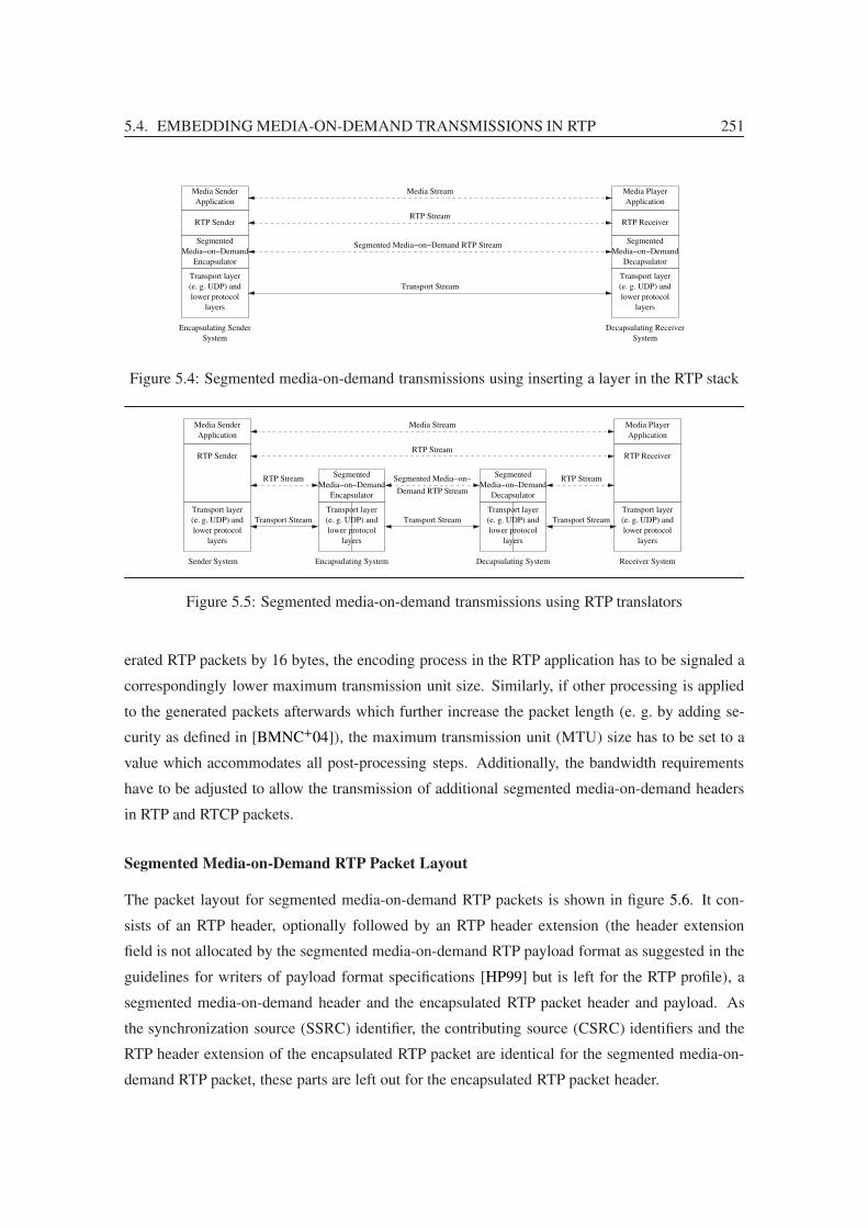
5.4. EMBEDDING MEDIA-ON-DEMAND TRANSMISSIONS IN RTP 251
Transport Stream
Segmented
Media−on−Demand
Encapsulator
Transport layer
(e. g. UDP) and
lower protocol
layers
RTP Sender
Media Sender
Application
Transport layer
(e. g. UDP) and
lower protocol
layers
Segmented
Media−on−Demand
Decapsulator
Media Player
Application
RTP Receiver
Media Stream
RTP Stream
Segmented Media−on−Demand RTP Stream
Encapsulating Sender
System
Decapsulating Receiver
System
Figure 5.4: Segmented media-on-demand transmissions using inserting a layer in the RTP stack
Decapsulating System
Media Sender
Application
Transport layer
(e. g. UDP) and
lower protocol
layers
RTP Sender
Media Player
Application
RTP Receiver
Transport layer
(e. g. UDP) and
lower protocol
layers
Segmented
Media−on−Demand
Encapsulator
Transport layer
(e. g. UDP) and
lower protocol
layers
Transport layer
(e. g. UDP) and
lower protocol
layers
Segmented
Media−on−Demand
Decapsulator
Media Stream
RTP Stream
Segmented Media−on−
Demand RTP Stream
RTP Stream RTP Stream
Sender System Receiver System
Transport Stream Transport Stream Transport Stream
Encapsulating System
Figure 5.5: Segmented media-on-demand transmissions using RTP translators
erated RTP packets by 16 bytes, the encoding process in the RTP application has to be signaled a
correspondingly lower maximum transmission unit size. Similarly, if other processing is applied
to the generated packets afterwards which further increase the packet length (e. g. by adding se-
curity as defined in [BMNC+04]), the maximum transmission unit (MTU) size has to be set to a
value which accommodates all post-processing steps. Additionally, the bandwidth requirements
have to be adjusted to allow the transmission of additional segmented media-on-demand headers
in RTP and RTCP packets.
Segmented Media-on-Demand RTP Packet Layout
The packet layout for segmented media-on-demand RTP packets is shown in figure 5.6. It con-
sists of an RTP header, optionally followed by an RTP header extension (the header extension
field is not allocated by the segmented media-on-demand RTP payload format as suggested in the
guidelines for writers of payload format specifications [HP99] but is left for the RTP profile), a
segmented media-on-demand header and the encapsulated RTP packet header and payload. As
the synchronization source (SSRC) identifier, the contributing source (CSRC) identifiers and the
RTP header extension of the encapsulated RTP packet are identical for the segmented media-on-
demand RTP packet, these parts are left out for the encapsulated RTP packet header.

252 CHAPTER 5. MEDIA TRANSPORT ENHANCEMENTS
Header Extension Len
Synchronization Source (SSRC) Identifier
Contributing Source (CSRC) Identifiers
...
RTP Header
0 31
Header Extension
...
RTP Header
Extension (opt.)
P X CC M PT Sequence Number
Timestamp
V=2
Playback Timestamp (fractional secs) Header
Media−on−Demand
Segmented
Slot Counter Playback Timestamp (seconds)
Absolute Sequence Number
Original Timestamp
Original Sequence Number
Padding (opt.) Padding (opt.) Padding Len (opt.)
RTP Payload Data
... Encapsulated
RTP Payload
Packet Header (stripped)
Encapsulated RTP
Header Extension Id
Figure 5.6: Segmented Media-on-Demand RTP packet format
RTP Header for Segmented Media-on-Demand Packets
The version field (V) is set to 2. The padding bit (P), the extension bit (X), the marker bit (M),
the synchronization source (SSRC) identifier, the contributing source identifier count (CC), the
contributing source (CSRC) identifiers and the RTP header extension are identical for segmented
media-on-demand RTP packets and the encapsulated RTP packets. The sequence number is set to
a random value for the first packet and is incremented by one (wrapping around on overflow) for
any further packet.
The assignment of an RTP payload type has to be performed in a dynamic way. The proposed
segmented media-on-demand payload format does not preserve the payload type of the encapsu-
lated media RTP packet (esp. in case of statically assigned payload types this is not recommend-
able), therefore a one-to-one mapping between the used payload type and the payload type of the
media RTP packet has to be set-up and signaled outside of RTP (e. g. using SDP, see section 5.5).
The timestamp is set to the absolute transmission time of the packet plus an initial startup
offset which is chosen randomly. Either the clock of the encapsulated media stream or a clock
with sufficient precision (e. g. 90 kHz) if the clock of the encapsulated data is unknown should be
used13.
Segmented Media-on-Demand Header
The segmented media-on-demand header contains the following fields:
13The used clock frequency must be signaled outside of RTP, e. g. using SDP (see section 5.5).
5.4. EMBEDDING MEDIA-ON-DEMAND TRANSMISSIONS IN RTP 253
Absolute Sequence Number: The absolute sequence number of the encapsulated RTP packet in
the original media stream transmission. The absolute sequence number must be independent
from the sequence number in the RTP header as the media-on-demand transmission scheme
may require repeated transmissions of segments. The absolute sequence number should
start with 0 at the beginning of the complete media stream and has to be incremented by
one for any further RTP packet14. If packet losses are detected at the encapsulation side, the
absolute packet number should reflect the losses if possible.
Slot Counter: This is a counter which is increased by one for each slot interval (and wraps around
on overflow). It can be used by the receiver system to locate slot boundaries which may
be necessary if the used transmission scheme requires that playbacks are delayed to slot
boundaries. The slot counter should start with a random value.
Playback Timestamp: As the unpacking process may have no knowledge of the used media
clock (and may have no access to sender reports to estimate it in case of encryption), this
timestamp provides the instant when the encapsulated packet has to be passed to the receiver
system. This timestamp uses a 65 536 Hz clock15 independent of the payload format of the
encapsulated RTP packet and starts with 0 at the beginning of the complete media stream.
Due to its size, the Playback Timestamp should not wrap around for a media-on-demand
transmission.
Segmented Media-on-Demand RTCP Packet Layout
The service provided by RTCP can be divided in two types for segmented media-on-demand trans-
missions: Some of the services should be provided end-to-end (e. g. sender reports which can be
used to synchronize several RTP streams to a common wall clock), others only within each of the
RTP sessions between sender, encapsulator, decapsulator and/or receiver (e. g. receiver reports).
While session-specific RTCP packets like receiver reports can be evaluated and handled sep-
arately for each of the RTP sessions (except if encrypted), end-to-end RTCP packets like sender
reports (esp. if encrypted) must be carried to the receivers without any change. To transfer these
RTCP packets from the sender to the receiver without interfering with the segmented RTP commu-
nication between the encapsulator and decapsulator, the RTCP packets have to be encapsulated in
a similar way as the RTP packets16. Figure 5.7 shows the layout of segmented media-on-demand
14This means that the absolute sequence numbers of a segmented media-on-demand transmission which is preceded
by a preloaded part does not start with 0 but continues the sequence numbers of the preloaded part. The same applies
to the playback timestamp.15A 65 536 Hz clock corresponds to an NTP [Mil92] clock as described in the RTP standard for wall clock timestamps
in RTCP sender report packets (omitting the least significant 16 bit). If the sender process can access the wall clock
timestamps of sender reports, this clock allows a simple interpolation.16Although sender reports can partly be reconstructed by the decapsulator from segmented media-on-demand RTP

254 CHAPTER 5. MEDIA TRANSPORT ENHANCEMENTS
packets which are used for this purpose. As requested by the RTP standard, an RTCP packet of
type “APP” is used for this purpose.
Packet Header (stripped)
P
0
V=2
31
LengthSubType=0 PT=APP=204
Synchronization Source (SSRC) Identifier
Name="SMOD"
Absolute Sequence Number
RTCP APP
Header
Header
Media−on−Demand
Segmented
PT specificRsvd.
Playback Timestamp (seconds)Slot Counter
Playback Timestamp (fractional secs)
Original PT
Padding (opt.) Padding (opt.) Padding Len (opt.)RTCP Payload
RTCP Payload Data
... Encapsulated
Encapsulated RTCP
Figure 5.7: RTCP packet format for encapsulated transmission of RTCP messages
RTCP Header for Segmented Media-on-Demand Packets
The version field (V) is set to 2. The padding bit (P) and the synchronization source (SSRC)
identifier are identical for segmented media-on-demand RTCP packets and encapsulated RTCP
packets. The subtype (SubType) is set to 0 and the packet type (PT) to APP=204. The length
field of the segmented media-on-demand RTCP packet is 4 higher than the length field of the
encapsulated RTCP packet. (The length field measures in units of 32 bit.) The Name field is set
to the ASCII representation of “SMOD” (as abbreviation of segmented media-on-demand).
Segmented Media-on-Demand Header
The segmented media-on-demand RTCP header contains the following fields:
Absolute Sequence Number: The absolute sequence number of the encapsulated RTCP packet
in the original media stream control transmission. The absolute sequence number has to
start with 0 and has to be incremented by one for any further segmented media-on-demand
RTCP packet.
Slot Counter: This is a counter which is increased by one for each slot interval (and wraps around
on overflow). It can be used by the receiver system to locate slot boundaries (even if no
RTP traffic is sent) which may be necessary if the used transmission scheme requires that
playbacks are delayed to slot boundaries. The slot counter should start with the same value
as the slot counter in the RTP data stream and should be increased synchronously with it.
packets by evaluating the playback timestamp, this reconstruction is incomplete (e. g. packet losses at the encapsulator
cannot be recorded in the sender reports) and impossible in case of encryption.
5.4. EMBEDDING MEDIA-ON-DEMAND TRANSMISSIONS IN RTP 255
Playback Timestamp: As the decapsulating process may have no knowledge of the used media
clock (and may have no access to sender reports to estimate it in case of encryption), this
timestamp provides the instant when the encapsulated packet has to be passed to the play-
back system. This timestamp uses a 65 536 Hz clock independent of the payload format of
the encapsulated RTCP packet and starts with 0 at the beginning of the whole media stream.
RTP/RTCP Packet Encapsulation Process
The sender shall perform the following steps to construct a segmented media-on-demand RTP
packet from an RTP packet of one RTP stream:
• Copy the RTP header, RTP extension header and payload data into the appropriate positions
of the segmented media-on-demand RTP packet. Thereby copy the sequence number and
timestamp of the RTP header and the payload data into the corresponding fields of the
encapsulated packet position.
• Replace the sequence number in the RTP header with the number one higher than the RTP
header sequence number of the last packet (or a random value for the first packet). Replace
the timestamp in the RTP header with the calculated instant when the RTP packet should be
transmitted, in units of the clock of the media stream if known or a 90 kHz clock otherwise.
At the beginning of the transmission, the timestamp should start with a random value.
• Calculate the playback time which corresponds to the timestamp of the RTP packet from
sender reports (if available and not encrypted), from the media timestamp (if the media
clock is known) or from the capturing instant and place it in the playback timestamp field of
the segmented media-on-demand header of the RTP packet. Place the least significant bits
of the current slot interval number in the slot counter field.
RTCP packets are processed in the same way.
RTP/RTCP Packet Decapsulation Process
The receiver has to keep the following context for the playback:
• The absolute sequence number of the next RTP packet to play,
• the absolute sequence number of the next RTCP packet to play,
• the current slot counter,
• a storage for RTP packets and
• a storage for RTCP packets.

256 CHAPTER 5. MEDIA TRANSPORT ENHANCEMENTS
The receiver shall perform the following steps when it receives a segmented media-on-demand
RTP packet:
• When a higher slot counter value than stored in the context is received (considering wrap
around on overflow), signal the start of a new slot boundary if the playback awaits this.
• If the absolute sequence number of the RTP packet is lower than the next absolute sequence
number to play or if a packet with the same absolute sequence number already exists in the
storage, ignore the packet.
• Reconstruct the encapsulated RTP packet from fields of the RTP packet and the encapsulated
RTP packet.
• Save the packet together with the absolute sequence number and playback timestamp in the
RTP packet storage.
Concurrently, it has to perform the following steps for playback:
• Check if the playback time for any unplayed packet in the storage has been reached17:
Therefore, calculate the playback time for all packets in the storage with an absolute se-
quence number greater or equal to the next absolute sequence number of the context by
adding the request time of the playback, the playback delay of the transmission (which has
to be transmitted outside of the scope of RTP, e. g. through the session description protocol
[HJP06], see section 5.5) and the playback timestamp. If the playback time for a packet has
been reached, play all RTP packets in the storage up to this packet and update the absolute
sequence number of the next packet to play in the context.
• If rewinding interactivity is not supported by the playback system, all played RTP packets
can be removed from the storage.
RTCP packets are processed in the same way.
Encryption and Forward Error Correction
Authentication and encryption [BMNC+04] as well as forward error correction [(Ed07] can be
applied to the segmented media-on-demand transmission to protect it. If forward error correction is
applied to the segmented media-on-demand transmission using [(Ed07], segment-based, channel-
based or transmission-based FEC can be achieved.
17The calculated playback time of RTP packet may be non-monotonic for some profiles if the synchronization time-
stamp is derived from the RTP media timestamp. For example in H.264, frames which are required to calculate interpo-
lated frames are transmitted in advance although their RTP timestamp is higher than the timestamp of the interpolated
frames. Therefore, it is not sufficient to examine only the playback time of the next packet to play. But in most cases it
should suffice to examine the next few packets instead of all unplayed packets.

5.4. EMBEDDING MEDIA-ON-DEMAND TRANSMISSIONS IN RTP 257
But it is also possible to tunnel an authenticated, encrypted and/or FEC-enhanced media stream
transparently through the segmented media-on-demand transmission encapsulation. This has been
made possible by a transparent transfer of media data independent of the payload type and by
preserving all fields of the RTP/RTCP packets. If forward error correction is applied to the original
media stream, the result corresponds to the stream-based FEC.
For encryption, it is more beneficial if it is applied after the transformation into a segmented
media-on-demand transmission, so the encapsulator has access to RTCP sender reports. Another
advantage if encryption is applied after the encapsulation (or a second time after encapsulation) is
that the encryption key can be changed for long-term segmented media-on-demand transmissions.
Extended RTP Profiles for RTCP-based Feedback
In [OWSB+06] and [OC08], RTP profiles are defined which allow receiver systems to give timely
feedback to sender systems. For segmented media-on-demand transmissions, this feedback cannot
be provided end-to-end because the lifetime of communication between sender system, encapsula-
tor, decapsulator and receiver system is independent from each other: For example, the encapsula-
tor may perform a segmented media-on-demand transmission for a long time, although the sender
system has finished the media stream transmission, and the decapsulator may continue stream-
ing the media stream data to the receiver system even if the encapsulator has already finished the
transmission.
For this reason, each of the translators should replace the “RTP/AVPF” or “RTP/SAVPF” pro-
file with “RTP/AVP” or “RTP/SAVP”, respectively, or vice versa, corresponding to the support
of feedback and security for their session.
5.4.3 Summary
This section proposed a simple but effective way how segmented media-on-demand transmissions
can be performed using the standardized real-time transport protocol RTP. Using a similar ap-
proach as SRTP, the plain media stream data is converted into a new format at the sender system
and back into the original stream at the receiver system. Nearly all of the benefits and extensions
which are available for RTP can be used for segmented media-on-demand transmissions, too, if
the proposed encapsulation scheme is used.
Besides of this, the proposed RTP payload format allows performing the conversion between
the original RTP media stream and the segmented media-on-demand RTP stream in separate sys-
tems. This gives the possibility for a smooth transition to segmented media-on-demand systems
as changes in existing applications are not necessary.
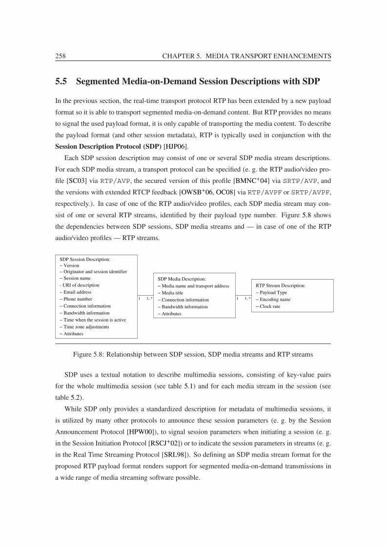
258 CHAPTER 5. MEDIA TRANSPORT ENHANCEMENTS
5.5 Segmented Media-on-Demand Session Descriptions with SDP
In the previous section, the real-time transport protocol RTP has been extended by a new payload
format so it is able to transport segmented media-on-demand content. But RTP provides no means
to signal the used payload format, it is only capable of transporting the media content. To describe
the payload format (and other session metadata), RTP is typically used in conjunction with the
Session Description Protocol (SDP) [HJP06].
Each SDP session description may consist of one or several SDP media stream descriptions.
For each SDP media stream, a transport protocol can be specified (e. g. the RTP audio/video pro-
file [SC03] via RTP/AVP, the secured version of this profile [BMNC+04] via SRTP/AVP, and
the versions with extended RTCP feedback [OWSB+06, OC08] via RTP/AVPF or SRTP/AVPF,
respectively.). In case of one of the RTP audio/video profiles, each SDP media stream may con-
sist of one or several RTP streams, identified by their payload type number. Figure 5.8 shows
the dependencies between SDP sessions, SDP media streams and — in case of one of the RTP
audio/video profiles — RTP streams.
SDP Session Description:
1 1..*
− Media name and transport address
− Media title
− Connection information
− Bandwidth information
SDP Media Description:
− Attributes
1 1..* − Encoding name
− Clock rate
RTP Stream Description:
− Payload Type
− Session name
- URI of description
− Email address
− Phone number
− Connection information
− Bandwidth information
− Time when the session is active
− Time zone adjustments
− Attributes
− Originator and session identifier
− Version
Figure 5.8: Relationship between SDP session, SDP media streams and RTP streams
SDP uses a textual notation to describe multimedia sessions, consisting of key-value pairs
for the whole multimedia session (see table 5.1) and for each media stream in the session (see
table 5.2).
While SDP only provides a standardized description for metadata of multimedia sessions, it
is utilized by many other protocols to announce these session parameters (e. g. by the Session
Announcement Protocol [HPW00]), to signal session parameters when initiating a session (e. g.
in the Session Initiation Protocol [RSCJ+02]) or to indicate the session parameters in streams (e. g.
in the Real Time Streaming Protocol [SRL98]). So defining an SDP media stream format for the
proposed RTP payload format renders support for segmented media-on-demand transmissions in
a wide range of media streaming software possible.

5.5. MEDIA-ON-DEMAND SESSION DESCRIPTIONS WITH SDP 259
Key Meaning of Value
v Version
o Originator and session identifier
s Session name
i Session information
u URI of description
e Email address
p Phone number
c Connection information for all media
b Bandwidth information for all media
t Time when the session is active
r Times of repetitions of the session
z Time zone adjustments
k Encryption key for all media
a Attributes for all media
Table 5.1: Session description parameters in SDP
Key Meaning of Value
m Media name and transport address
i Media title
c Connection information
b Bandwidth information
k Encryption key
a Attributes
Table 5.2: Media description parameters in SDP
5.5.1 Requirements for an SDP Media Stream Format Description for Segmented
Media-on-Demand
The SDP media stream format description for the segmented media-on-demand RTP payload for-
mat has to fulfill the following requirements:
1. The media stream format description should comply fully to the SDP standard.
2. The media stream format description should cover all media-on-demand specific transmis-
sion parameters (e. g. for playback delay, partial preloading).
3. The original payload format should be encapsulated in the new media stream format de-
scription.
4. Other RTP profiles and payload formats, e. g. forward error correction and security, should
be combinable with segmented media-on-demand transmissions.

260 CHAPTER 5. MEDIA TRANSPORT ENHANCEMENTS
The ability to convert a media stream description is very important as only this allows translat-
ing an RTP media stream together with its description into the segmented media-on-demand RTP
payload format and back into its native payload format.
5.5.2 SDP Media Stream Format Description for Segmented Media-on-Demand
To signal the payload format of media streams in SDP using the RTP/AVP profile or one of its
variants, either a statically assigned payload type number can be used or the assignment can be
done dynamically using an “a=rtpmap:” attribute. The “a=rtpmap:” attribute thereby is
assembled in the following way:
a=rtpmap: 〈payload type〉 〈encoding name〉/〈clock rate〉[/〈encoding parameters〉]
〈payload type〉: The payload type number for which to specify a mapping.
〈encoding name〉: The name of the payload format used for the encoding.
〈clock rate〉: The clock rate of the encoding.
〈encoding parameters〉: Arbitrary encoding parameters.
Examples (extended excerpt from [HJP06]) for this are given in figure 5.9.
Session level information:
v=0o=bn 3417930927 3417930927 IN IP4 83.246.72.241s=SDP Examplei=Example showing SDP [email protected]=3417930927 3417930927a=recvonly
Statically assigned payload format:
m=audio 49232 RTP/AVP 0c=IN IP4 224.2.3.4/127
Dynamically assigned payload format:
m=audio 49233 RTP/AVP 96c=IN IP4 224.2.3.5/127a=rtpmap:96 L16/16000/2
Several payload formats:
m=audio 49232 RTP/AVP 97 98 99c=IN IP4 224.2.3.6/127a=rtpmap:97 L8/8000a=rtpmap:98 L16/8000a=rtpmap:99 L16/11025/2
Figure 5.9: Example media specifications in SDP

5.5. MEDIA-ON-DEMAND SESSION DESCRIPTIONS WITH SDP 261
To use the segmented media-on-demand payload format, only the dynamically assigned pay-
load type specification can be used because the segmented media-on-demand payload format has
not yet been statically assigned in any RTP profile. To translate a media description with a stati-
cally assigned payload format into one using the segmented media-on-demand payload format, an
unused payload type number must be searched and substituted for the statically assigned payload
type.
As a next step, the payload format has to be changed to “SMOD” (segmented media-on-demand)
and the clock rate should be set to 90 kHz if it is unknown. Thereby the original payload format
must be preserved so the decapsulator can signal the original payload format to the application
later. The standard states that
encoding parameters added to an “a=rtpmap:” attribute SHOULD only be those
required for a session directory to make the choice of appropriate media to participate
in a session
and that other parameters should be added in other attributes. As the original payload format is
important for the choice of the appropriate media, it must be added as encoding parameter to the
“a=rtpmap:” line. For this, the following format will be used for the 〈encoding parameters〉 of
the “a=rtpmap:” line:
• If a statically assigned payload type had been used (which has been converted into a dynamic
one as described above):
static/〈original payload type〉
• If a dynamically assigned payload type had been used:
dynamic/〈original encoding name〉/〈original clock rate〉[/〈original encod-
ing parameters〉]
Some other fields of the session description must be updated when translating a session de-
scription into one using segmented media-on-demand transmissions at the encapsulator or back to
the original format at the decapsulator:
• The “c=” connection field should be updated by the encapsulator and decapsulator: Firstly,
for the segmented media-on-demand transmission, multicast addresses should be used, so
several decapsulators can receive the transmission. But even if multicast addresses have
already been used by the sender, these addresses should be exchanged by other multicast
addresses to prevent that the original media streams are routed to the decapsulators18 . The
18If the sender, encapsulator and decapsulator all use different IP addresses, source-specific multicast routing could
also be used if utilized by all participants.

262 CHAPTER 5. MEDIA TRANSPORT ENHANCEMENTS
decapsulator should replace the multicast addresses either by one other set of addresses per
receiver or use its own unicast address. Additionally, the port numbers in the “m=” media
formats must be updated so they are (at least for equal connection addresses) unique.
• The “t=” timing and “r=” repeat times fields should be adjusted to reflect the segmented
media-on-demand transmission: The timing field should be updated to indicate the start
and end of the segmented media transmission and the repeat times field should signal any
scheduled repetitions of the segmented media-on-demand transmission. Any existing “z=”
zone offset must be replaced according to time zone adjustments which occur during the
segmented media-on-demand transmission (which may take place at a different time than
the original transmission). The decapsulator will derive the “t=” timing for the playback
using the media playback time as start time and calculating the end time from the duration
in the “r=” repeat time field.
• The “b=” bit rate field should be updated to reflect the overhead of the segmented media-
on-demand RTP encapsulation. To allow reconstruction of the original values after decap-
sulation, the original values should be transmitted in “a=smod-b:” attributes.
• The “o=” origin field contains a globally unique identification of the session and a version
number for the session. As each translator forwards data from one RTP session into another
one, the sessions must be named differently.
• An “a=recvonly” attribute should be added if not already present. “a=sendrecv”
attributes should be deleted. (If an “a=sendonly” attribute is present, this should be
considered as an error.)
Playback Delays
In addition to the above described modifications to standard parameters, some media-on-demand
specific attributes must be added to the media description.
To indicate the playback delay to the decapsulator, the minimum and maximum playback delay
are encoded using an “a=smod-delay:” media stream attribute. This attribute is defined as
follows:
a=smod-delay: 〈minimum delay〉 [〈maximum delay〉]
〈minimum delay〉: The minimum playback delay in clocks of the segmented media-on-demand
media stream.
〈maximum delay〉: The maximum playback delay in clocks of the segmented media-on-demand
media stream. The maximum playback delay actually works as a flag, indicating if the
playback should start with 〈minimum delay〉 after a slot boundary has been reached. The

5.5. MEDIA-ON-DEMAND SESSION DESCRIPTIONS WITH SDP 263
signaled value can be used to indicate the maximum playback delay to the user or to imple-
ment a timeout. If minimum and maximum playback delay equal in the used transmission
scheme (see section 4.9), the maximum value must be omitted or set to the same value as
〈minimum delay〉.
Note that the Playback Timestamps in the segmented media-on-demand RTP packets are
always starting with 0 at the beginning of a media stream, any delays which are specific to the
scheduling parameters are signaled in SDP. This has the advantage that the scheduling parameters
can be changed dynamically (see section 4.15 and 4.16) without updates in the segmented media
stream, a prerequisite for not interrupting ongoing transmissions.
Partial Preloading
Partial preloading consists of two processes: The preloading of a part of the media stream and the
playback of a preloaded media stream as part of a segmented media-on-demand transmission.
Although preloading does not require real-time transmission and can be performed e. g. using
content distribution systems, this section describes a way to transfer the preloaded part of a media
stream using RTP for convenience19 .
For the preloading process, a means to signal the preloading (and thus storing the media stream)
is required. This is indicated by an “a=smod-preload:” attribute in the media description:
a=smod-preload: 〈payload type〉 〈expiry time〉 〈username〉 〈preload-id〉〈preload-version〉 〈nettype〉 〈addrtype〉 〈unicast-address〉
〈payload type〉: The payload type number of the media stream which is to be preloaded. The
content is named separately for each payload type during preloading so it is possible to
associate multiple streams with their continuation at playback.
〈expiry time〉: The time when the preloaded data can be dropped because it is not needed any
more. This value is the decimal representation of a Network Time Protocol (NTP) [Mil92]
time value in seconds since 1900.
〈username〉: The user’s login on the originating host, or “-” if the originating host does not sup-
port the concept of user IDs.
〈preload-id〉: A numeric string such that the tuple of 〈username〉, 〈preload-id〉, 〈nettype〉,〈addrtype〉, and 〈unicast-address〉 forms a globally unique identifier for the preloaded data.
The method of 〈preload-id〉 allocation is up to the creating tool, but Network Time Protocol
(NTP) [Mil92] format timestamps are suggested to ensure uniqueness.
19If preloaded parts are transmitted using other means, the proposed naming scheme must be followed, so receiver
systems are able to insert the media stream on playback.

264 CHAPTER 5. MEDIA TRANSPORT ENHANCEMENTS
〈preload-version〉: A version number for the preloaded data. Its usage is up to the creating tool,
so long as 〈preload-version〉 is increased when a modification is made to the preloaded data.
Again, it is recommended that an NTP format timestamp is used.
〈nettype〉: A text string giving the type of network, e. g. “IN” for “Internet”.
〈addrtype〉: A text string giving the type of address that follows, e. g. “IP4” or “IP6”.
〈unicast-address〉: The address of the machine on which the preloaded data was created.
The above attributes assure that the preloaded media stream data is uniquely named (using the
same approach as SDP uses for the “o=” origin field), has a version number (so the decapsu-
lator can replace old versions with new ones) and an expiry date (to enable the decapsulator to
delete the preloaded data after some time). When the decapsulator receives a media stream with
the “a=smod-preload:” present, it should save the media stream together with the media
description for later playback.
To request playback of a preloaded media stream at the beginning of a segmented media-on-
demand transmission20, an “a=smod-insert:” attribute is used:
a=smod-insert: 〈payload type〉 〈username〉 〈preload-id〉 〈preload-version〉〈nettype〉 〈addrtype〉 〈unicast-address〉
〈payload type〉: The payload type number of the media stream where to insert the preloaded part
of the media stream.
〈username〉, 〈preload-id〉, . . . : Identification of the preloaded part.
Example
Figure 5.10 shows the result of this procedure for the above given examples, using a (minimum
and maximum) playback delay of 10 seconds, and figure 5.11 shows an example using a 10 second
partial preloading.
5.5.3 Summary
SDP is a commonly used specification to describe session parameters, esp. in combination with
RTP. Specifying a media format description for the previously proposed RTP payload format com-
pletes the payload format specification and supports the use of the segmented media-on-demand
RTP payload format in a wide range of media streaming applications.
20Only preloading to the beginning of a media stream is supported with this attribute; introducing breaks into a media
stream which are filled with preloaded data is out of the scope of SDP.

5.6. CONCLUSION 265
Session level information:
v=0o=bn 3417930927 3417930927IN IP4 83.246.72.241
s=SDP Examplei=Example showing SDP [email protected]=3417930927 3417938127a=recvonly
Statically assigned payload format:
m=audio 49232 RTP/AVP 0c=IN IP4 224.2.3.4/127
Dynamically assigned payload format:
m=audio 49232 RTP/AVP 96c=IN IP4 224.2.3.5/127a=rtpmap:96 L16/16000/2
Several payload formats:
m=audio 49232 RTP/AVP 97 98 99c=IN IP4 224.2.3.6/127a=rtpmap:97 L8/8000a=rtpmap:98 L16/8000a=rtpmap:99 L16/11025/2
(a) Example media specifications in SDP
Session level information:
v=0o=bn 3417930937 3417930937
IN IP4 83.246.72.242s=SDP Examplei=Example showing SDP [email protected]=3417930927 3420522927r=10 7200 0a=recvonly
Statically assigned payload format:
m=audio 49232 RTP/AVP 100c=IN IP4 224.2.4.4/127a=rtpmap:100 SMOD/90000/static/0a=smod-delay:100 900000
Dynamically assigned payload format:
m=audio 49232 RTP/AVP 95c=IN IP4 224.2.4.5/127a=rtpmap:96 SMOD/16000/dynamic/L16/16000/2a=smod-delay:96 160000
Several payload formats:
m=audio 49232 RTP/AVP 97 98 99c=IN IP4 224.2.4.6/127a=rtpmap:97 SMOD/8000/dynamic/L8/8000a=rtpmap:98 SMOD/8000/dynamic/L16/8000a=rtpmap:99 SMOD/11025/dynamic/L16/11025/2a=smod-delay:97 80000a=smod-delay:98 80000a=smod-delay:99 110250
(b) Translated segmented media-on-demand media specifica-
tions in SDP
Figure 5.10: Media specifications in SDP
5.6 Conclusion
In this chapter, several enhancements have been proposed which can be applied to media-on-
demand transmissions independent of the used transmission scheme:
To handle partial loss of data of a transmission, several treatments have been described, one
reactive (ARQ-based error recovery), one pro-active (FEC) and the combination of these two
approaches (HARQ-based error recovery). It has been analyzed that it is more efficient to apply
forward error correction to the media stream directly instead of applying it to the sequence of
segments which are sent on one or all channels.
To support systems with low receiver bandwidth, modifications to the Generalized Greedy
Broadcasting scheme have been proposed in the previous chapter. Another approach is to use
layered encodings where the media stream is split into a common, base-quality part and one or

266 CHAPTER 5. MEDIA TRANSPORT ENHANCEMENTS
Preloading:
v=0o=bn 3417930927 3417930927 IN IP4 83.246.72.242s=SDP Examplei=Example showing SDP [email protected]=3417930927 3417930987a=recvonly
m=video 49152 RTP/AVP 96c=IN IP4 224.2.4.4/127a=rtpmap:96 SMOD/90000/dynamic/H264/90000a=smod-preload:96 3420522927 bn 3417930927 3417930927 IN IP4 83.246.72.241
Playback inserting preloaded data into a transmissions:
v=0o=bn 3417934537 3417934537 IN IP4 83.246.72.242s=SDP Examplei=Example showing SDP [email protected]=3417934587 3420522987r=1 7200 0a=recvonly
m=video 49153 RTP/AVP 97c=IN IP4 224.2.4.5/127a=rtpmap:97 SMOD/90000/dynamic/H264/90000a=smod-delay:97 0a=smod-insert:97 bn 3417930927 3417930927 IN IP4 83.246.72.241
Figure 5.11: Segmented media-on-demand media specifications using partial preloading
several enhancing parts. Depending on the available bandwidth, the receiver system can decide
how much of these streams are received.
To protect the media stream transmission, several security related issues have been addressed:
Encryption for confidentiality, signing for authenticity and integrity, and watermarking for recog-
nition of unlicensed copies. As an alternative approach to encryption, chaffing and winnowing has
been proposed and extended to lower the bandwidth requirements of receiver systems.
To assist embedding of segmented media-on-demand transmissions in current environments,
a payload format for the real-time transport protocol RTP and a media format specification for
the proposed payload format in SDP have been defined: Using the segmented media-on-demand
payload format, it is possible to transmit segmented media-on-demand transmissions of all size-
based and frequency-based transmission schemes while benefiting from the capabilities of the
real-time transport protocol at the same time.
Additionally, the proposed RTP payload format can be implemented in separate systems. This
allows extending existing RTP-based media-on-demand system to support segmented media-on-
demand transmissions using any size- or frequency-based segmented transmission scheme (e. g.

5.6. CONCLUSION 267
the Generalized Greedy Broadcasting scheme proposed in chapter 4) including the other above
described enhancements without changing the existing system.


Chapter 6
Analysis of Media-on-Demand
Application Cases
THIS chapter presents an analysis of the cost-effectiveness of different media-on-demand ap-
proaches in various application cases. Instead of differentiating the proposed media trans-
mission schemes by their requirements or efficiency as done in chapter 3, their costs and benefits
are balanced against each other in this chapter.
After starting with some basic calculations about cost analysis for media-on-demand in the
next section, three application cases of different size are examined in sections 6.2 to 6.4, resp. This
examination in three groups of different size is commendable due to the effects on the number of
receiver systems and bandwidth availability:
• In small environments, media-on-demand systems have to serve only a low number of re-
ceiver systems while typically a high bandwidth is available. Typical small environments
for media-on-demand systems can be found in hotels, air planes, trains, ships or blocks of
houses.
• Larger installations, e. g. hotel chains, large companies or small villages, are examined in the
group of medium-sized environments. They differ from the small environments by a higher
number of receiver systems and less available (or at least more expensive) bandwidth.
• Distribution of media streams to a huge number of receiver systems, e. g. to cities or even
whole countries, with low bandwidth availability, are examined in the large environment
case.
The last section of this chapter gives a summary of the used media-on-demand transmission
schemes which have been evaluated to be favored in each of the cases.

270 CHAPTER 6. ANALYSIS OF APPLICATION CASES
6.1 Cost Analysis of Media-on-Demand Systems
As stated above, the comparison in this chapter is driven purely by financial aspects. Therefore, it
is most important to analyze the business model for media-on-demand and evaluate costs and rev-
enue. In the following subsections, the foundation for the cost analysis are observed, starting with
the value chain for media-on-demand in section 6.1.1, continuing with a layout of preconditions
which are assumed in the analysis in section 6.1.2 and finishing with a composition of costs and
revenue for media-on-demand providers in section 6.1.3.
6.1.1 Value Chain
The value chain for media-on-demand involves a series of players [Poi04]: Starting with the con-
tent providers who originate the media streams, aggregators negotiate distribution rights and mar-
ket packages of media streams to service providers. The service providers then distribute the media
streams to the end users using a network infrastructure which may be owned by yet another party.
Table 6.1 gives a more detailed overview of the participants in the value chain, their function and
some well-known examples.
Player Role Examples
Content Provider (movie
studio, broadcaster, inde-
pendents)
Commission, production, marketing; own
and develop the brand, own the copyright
Disney, Time Warner, BBC,
MTV, Star, CNN, Fox Kids,
. . .
Content Aggregator Encoding and managing media-on-demand
content, negotiate rights with multiple
content providers, market complete pack-
age and deliver it to e. g. video service
providers
FastWeb, Anytime, Arrivo,
ODG
Service Providers Manage and deliver media-on-demand
(and other media services) to end-users,
perform billing with end-users
FastWeb, Broadmedia, KIT,
Video Networks
Broadband network opera-
tors
Provide network infrastructure to transmit
media streams
FastWeb, Yahoo! Japan,
France Telecom, BT, Com-
cast
End-user Consumes the media streams
Table 6.1: Value chain for media-on-demand
The splitting of revenue across the players of the value chain is still contentious. For tradi-
tional video broadcast, often a split of 50:25:25 for content provider, content aggregator and video
service provider (where the service provider pays for the broadband network) is quoted [Poi04],
but the actual split varies greatly from country to country. For the most valuable media streams,
content providers will often demand 60 % or even more of the revenue. Additionally, some play-

6.1. COST ANALYSIS OF MEDIA-ON-DEMAND SYSTEMS 271
ers choose to occupy multiple positions in the value chain, making these estimations even more
difficult.
For media-on-demand, the division may change as the network costs are significantly higher.
The authors of [Moo05] state that a split of 60:40 for content provider and content distributor is yet
commonly used in the context of video-on-demand but this change of the established split is one
of the reasons which causes the major content providers to be concerned about media-on-demand.
New media-on-demand transmission schemes may be a way to lower the transmission costs, both
increasing the revenue for the content provider and the service provider and preventing a failure
of this type of service due to discordance of the split to apply.
6.1.2 Preconditions
In the cost analysis of this chapter, the following preconditions are assumed:
Number of connected receiver systems: As mentioned above, this analysis covers three appli-
cation cases of different size: For the small environment, it is assumed that 200 receiver
systems are connected to the media-on-demand system, for medium-sized installations,
20 000 receiver systems are assumed and for the large installation, the analysis is based
on 2 000 000 connected media-on-demand receiver systems.
Peak usage: In lifelike environments, it is very improbable that all connected media-on-demand
receiver systems are receiving a media stream at the same time. But as the bandwidth
of reactive media-on-demand transmission schemes has to be calculated depending on the
number of concurrently active systems, some assumptions have to be made about:
For small environments (e. g. in hotels, planes or trains), it is assumed that 160 receiver
systems are receiving data from the media-on-demand system concurrently, for medium-
sized environments 5 000 concurrently active receiver systems are assumed and for large
environments 500 000 receiver systems can be concurrently active. This corresponds to a
concurrent usage rate of 80 % for small environments and 25 % for medium-sized and large
environments [Poi04].
Please note that the number of active receiver systems may also differ depending on the place
of installation (e. g. in planes the offer may be used more intensive and more simultaneously
than in hotels) and on the popularity of the service.
Request pattern: It is assumed that media stream requests follow the Zipf distribution with a
parameter of 0.729 (see section 3.1.1).
Media Type: This analysis only examines the most popular type of media-on-demand: The on-
demand transmission of audio-visual content, essentially movies.

272 CHAPTER 6. ANALYSIS OF APPLICATION CASES
Media Quality: As more and more customers have been indulged by the media quality of DVD
and CD, they expect a high video and audio quality for media-on-demand, too. But as
bandwidth requirements are an important cost factor, a video quality slightly below DVD
and a moderate audio quality are presumed to fulfill the customers’ demands.
Media Bit Rate: The media bit rate depends on the video compression scheme and the compres-
sion rate which determine the video quality. Using MPEG-2 video encoding, 1.5 Mbit/s
corresponds nearly to VHS quality while DVDs typically use 3–10 Mbit/s in variable-bit-
rate encoding. If H.264/MPEG-4 Part 10/AVC is used instead, the bit rate can be reduced by
a factor of two to three [GC01], resulting in an average bit rate of roughly 1.5–3 Mbit/s for
DVD video quality. Thus for this analysis, an average media bit rate of 2 Mbit/s is assumed.
Reactivity: Both pro-active and reactive environments are examined.
Multicasting: For pro-active environments, a multicast-capable network is assumed, for reactive
environments, multicasting is not considered in this analysis.
Transmission Schemes: This analysis focuses on two transmission schemes: Point-to-Point
transmission scheme and the Generalized Greedy Broadcasting Scheme. Point-to-Point
transmissions have been selected for several reasons: On the one hand, they are very com-
mon in the context of media-on-demand (nearly all media-on-demand services currently
available are based on Point-to-Point transmissions, see appendix E), on the other hand,
they place very few requirements on the receiver systems. As alternative to this simple
transmission scheme, the newly proposed Generalized Greedy Broadcasting scheme has
been selected because of its high efficiency and general utilizability.
Although it is known that multicast-based transmission schemes perform better than unicast-
based ones if the multicast data is received by several receiver systems at once [CC01], the
sender and receiver system requirements are higher for multicast-based systems. Through
this analysis, the threshold when the bandwidth savings of a multicast-based system over-
weight the increase in complexity and costs of multicast-based transmission schemes are
examined.
Additionally, a hybrid setup is examined where the seldom requested media streams are sent
using Point-to-Point transmissions and often requested media streams using the Generalized
Greedy Broadcasting Scheme.
Media assortment: In environments where the customers only stay relatively short (e. g. hotels,
air planes, trains or ships), a small media assortment (around ten media streams) is most
probably sufficient. In other installations (e. g. media-on-demand systems for home en-
tertainment), a larger assortment (e. g. with several thousands of media streams) may be
necessary to accomplish customer demands.

6.1. COST ANALYSIS OF MEDIA-ON-DEMAND SYSTEMS 273
This analysis compares the results for media assortments of the different sizes between 10
and (where applicable) 1 000 media streams, detailing the calculations for 20 titles for the
small environment, 50 titles for the medium-sized setup and 200 titles for the large installa-
tion.
Partial preloading: Partial preloading can be used to reduce bandwidth requirements as de-
scribed in section 4.6. For this analysis, the case that no, a fraction of 160
or a fraction
of 112
of the media streams are preloaded are examined. For the latter two cases, 30 GB or
150 GB of additional storage are required if the beginnings of 1 000 media streams of an
average media bit rate of 2 Mbit/s are preloaded, resp.
Playback Delay: Many of the more efficient transmission schemes (and all pro-active schemes
which do not use partial preloading) cannot provide immediate service; the customers have
to wait for a playback to commence. As customers may refuse the service if they have to
wait too long for the media playback and as they may have been indulged from media-on-
demand services with immediate service, a new service must accomplish a short playback
delay to be competitive.
Thus, this analysis covers the results for three different playback delays: The results for
immediate service (if possible), for playback delays of 1120
and for delays of 160
of the media
stream duration are examined (where the latter two correspond to playback delays of one
and two minutes for a two hour media stream, resp.).
As it is assumed that media streams are typically requested in a Zipf-distribution like manner
(see above), it may be reasonable to accommodate the playback delay to the request rate:
Therefore, an alternative setting is evaluated, too, where the most popular 5 % of all media
streams are served with immediate service, the next 20 % of the media streams in popularity
with a playback delay of 1120
and the remaining media streams with a playback delay of
160
. Using this partitioning, about 31 % of all requests are served with a playback delay
of 1120
of the media stream duration, another 30 % with a playback delay of 160
and the
remainder with a delay of 124
, resulting in an average playback delay of 0.009 · d (which
equals approximately 64.8 seconds for a two hour media stream).
Breaks: No breaks are introduced to the media stream transmissions.
Error Correction: It is assumed that no ARQ-based error recovery but only forward error cor-
rection is performed. Therefore, 5 % redundancy data is added to the transmission.
Protocol Overhead: When transmitting media data, each protocol in the used protocol stack adds
some data and thus increases the bandwidth requirements. For example, to send media
stream data using segmented media-on-demand RTP (see section 5.4) over UDP and IP,
56 octets overhead per RTP packet are produced. For 1 500 octet IP packets, this results in

274 CHAPTER 6. ANALYSIS OF APPLICATION CASES
an overhead of 3.73 %, thus a gross media bit rate (including FEC and protocol overhead)
of 2.178 Mbit/s is used for the following calculations.
Bandwidth Requirements: To analyze the costs of a transmission, the bandwidth requirements
have to be determined beforehand: According to the examination of transmission schemes
in chapter 3 and 4, the media bit rate, the bandwidth requirements of the used transmission
scheme and the desired playback function influence the required bandwidth.
Depending on the transmission scheme, a multiple of the media bit rate is needed to get the
transmission bandwidth:
• In environments which do not support multicasting, only Point-to-Point transmissions
can be used. In this case, the maximum needed bandwidth at the sender system is
the product of the number of concurrently active receiver systems and the gross media
bit rate (2.178 Mbit/s). Table 6.2 shows the resulting bandwidth requirements for the
Point-to-Point Transmission scheme for the described setups.
• Table 6.3 shows the data for the Generalized Greedy Broadcasting scheme for all se-
tups specified above. In all cases, the sender bandwidth is much lower compared to the
Point-to-Point transmission scheme because of the high efficiency of the Generalized
Greedy Broadcasting scheme, but the requirements on the receiver systems are higher.
Storage size of receiver systems: For the Generalized Greedy Broadcasting scheme, it is as-
sumed that receiver systems provide space for storing up to about 43 % of the media stream
(which corresponds to about 774 MB in case of a two hour media stream of an average
bit rate of 2 Mbit/s). In case of partial preloading, additional storage space is necessary as
described above.
Network type: Depending on the size of the environment, different types of networks are used.
In small environments, a local area network (e. g. based on Ethernet) provides enough band-
width: If Point-to-Point transmissions are used to transmit media streams of 2.178 Mbit/s,
Size of Number of Total bw.
environment active rcv. in Mbit/s
Small 160 347.7
Medium 7500 16297.5
Large 200000 434600.0
Table 6.2: Bandwidth requirements for Point-to-Point transmissions

6.1. COST ANALYSIS OF MEDIA-ON-DEMAND SYSTEMS 275
Playback Amount of Req. ch. Avg. bw.
delay preloading per stream per stream.
in Mbit/s
0 d60
4.12 8.98
0 d12
2.50 5.45d
1200 4.84 10.54
d120
d60
3.72 8.10d
120d12
2.41 5.25d60
0 4.14 9.02d60
d60
3.44 7.49d60
d12
2.33 5.07
varying d60
varying 7.75
varying d12
varying 5.12
Table 6.3: Bandwidth requirements for Generalized Greedy Broadcasting transmissions
100 Mbit/s Ethernet can accomplish 34 transmissions and 1 Gbit/s Ethernet allows trans-
mitting 344 media streams (assuming a network utilization of 75 % in both cases1).
For transmissions using the Generalized Greedy Broadcasting scheme, a bandwidth of up
to 10.52 Mbit/s is required for each media stream (see table 6.3). This limits the number of
broadcasts which can be sent on 100 Mbit/s Ethernet to seven and on 1 Gbit/s Ethernet to 71
for this case (again assuming a network utilization of 75 %). The network layout is more
complicated, too, but if no media-on-demand sender system provides more than 71 media
streams and no switch where receiver systems are connected to serves more than 71 receiver
systems, it is sufficient to connect all media-on-demand sender systems and switches to a fast
“root” switch via 1 Gbit/s which has a backplane of at least 3 Gbit/s to support 200 receiver
systems. Figure 6.1 illustrates this setup.
Wireless local area networks which provide enough bandwidth for the described media-
on-demand application cases are not yet available and thus not included in this analysis:
Currently, IEEE 802.11g only provides three and IEEE 802.11a eight non-overlapping
20 MHz bands, each providing a gross bit rate of 54 Mbit/s and a net bit rate (after re-
moving physical and data link layer overhead) of 37 Mbit/s2. Assuming a media stream
of 2.178 Mbit/s and a network utilization limit of 75 %, 12 concurrent Point-to-Point trans-
missions or 2 Generalized Greedy-based stream transmissions are possible on each band.
Unfortunately, these bit rates are not achievable in practical environments, esp. inside build-
1A network utilization of 75 % should be possible in this setup if switched Ethernet is used, but if other traffic than
media-on-demand is also served through this network, precautions have to be taken.2IEEE 802.11n (standardization not finished yet) will allow wireless local networks reach bandwidths of up to
300 Mbit/s with a net throughput of up to 100 Mbit/s, which may become more interesting for media-on-demand.

276 CHAPTER 6. ANALYSIS OF APPLICATION CASES
(max. 71 Titles per System)
.. .
Media−on−Demand
Receiver Systems
(1 Gbit/s uplink)
100 Mbit/s−Switches
1 Gbit/s−Switch
(3 Gbit/s backplane)
Media−on−Demand
Sender Systems
(max. 71 per Switch)
Figure 6.1: Structure for a setup where the Generalized Greedy Broadcasting scheme can be used
to serve 200 receiver systems using 100 Mbit/s and 1 Gbit/s Ethernet only
ings, where this bit rate decreases rapidly for distances above 25 meters. Therefore, the use
of wireless local area networks is not applicable for the analyzed environments.
Medium-sized environments require larger types of networks, e. g. metropolitan to wide
area networks or several interconnected small networks. Examples for suitable metropoli-
tan and wide area networks are based on Asynchronous Transfer Mode (ATM) networks
[Rig98, Gin96a] (currently limited to 2 488 Mbit/s if used for IP transmissions due to
the technical complexity from segmentation and reassembly for IP packets in ATM cells),
Packet over SDH/SONET (POS) [MS99] (up to 10 Gbit/s if used for IP transmission) or
Metro Ethernet [San03] (up to 10 Gbit/s, too). Approaches to use ATM without the Internet
layer for media-on-demand [Gin96b] — either in point-to-point or in point-to-multipoint
mode — have not spread widely due to missing ATM connectivity of private households.
If households have to be connected to a broadband network, installation is expensive if not
performed on top of existing infrastructure: For example, in case of DSL (Digital Subscriber
Line)-based Internet access, the high frequency spectrum of coppery telephone lines is used
to transmit data between the telephone central office and households. (Other examples for
data transmission over existing infrastructure are Internet over cable TV networks or over
power lines.)
Major parts of the Internet are not multicast-capable yet, so at a first glance, it looks ques-
tionable if multicast-based media-on-demand transmission systems can be used in this sce-
nario. But fortunately, it is not required that the whole Internet is multicast-capable but just
the DSL access concentrator: For DSL-based Internet access, the media-on-demand sender
system can be placed at the DSL access concentrator3 and communicate with all receiver
3DSL lines are typically not connected to the Internet at the central office: At the central office, the DSL traffic is
6.1. COST ANALYSIS OF MEDIA-ON-DEMAND SYSTEMS 277
systems which are bound to this access concentrator4 . The number of systems which can be
reached this way depends very much on the number of DSL customers and the number of
DSL access modulators which are connected to the access concentrator. In case of Deutsche
Telecom AG, 74 DSL access concentrators are used to connect around 5 million DSL cus-
tomers (as of year 2004), so roughly 67 000 systems can be reached in average at each access
concentrator which matches roughly the medium-sized environment case. Alternatively, if
the media-on-demand server cannot be placed directly at the DSL access concentrator, a
multicast tunnel can be established from the media-on-demand sender systems to the DSL
access concentrator.
Deutsche Telecom AG also started to install Outdoor-DSLAM systems which provide up
to 50 Mbit/s in downstream to the home. These systems are equipped with IPTV-aware
VDSL2 hardware which already supports multicast in downstream direction.
As DSL and similar techniques like the aforementioned cable TV or power line Internet
access methods provide currently the best affordable high-speed Internet access which is
usable for media-on-demand, DSL-based Internet access has been selected for medium-
sized environments.
For large environments, it is nearly impossible to circumvent wide area networks. One type
of wide area networks which is already popular for traditional media transmissions is built
by satellites: Satellites allow to transmit data to all inhabitants of a country or even continent
at once and thus fit with ease in the large-sized environment case.
Alternatively, DSL-based Internet access can be used in large environments, too: In this
case, media-on-demand sender systems can be placed at several DSL access concentrators
or a single media-on-demand service location can be selected which sends the media streams
to all access concentrators.
6.1.3 Costs and Revenue of Media-on-Demand
This subsection examines the different types of costs and sources of revenue for media-on-demand
providers and estimates their amounts which are used for the calculations in the next three sections.
only split from the telephone lines using DSL access modulators and then sent (e. g. via ATM, sometimes also using
fiber GBit-Ethernet) to the access concentrator where routing to the Internet is performed.4Some DSL-based video broadcast systems already utilize multicasting for sending television data over DSL, e. g.
the mPhaseTV+ platform, consisting of an mPhase Broadcast Television Switch (mPhase Technologies) and a Stinger
DSL Access Concentrator (Lucent Technologies).

278 CHAPTER 6. ANALYSIS OF APPLICATION CASES
Costs for Providing Media-on-Demand
The costs for providing a media-on-demand service can be divided in two parts: Some of the costs
are general to any media-on-demand service, others depend on the used transmission technique.
Although the comparison is just based on the costs which depend on the used transmission
technique, other costs are given here as found in literature for completeness:
Sender system equipment: For sending media streams to end-users, the service provider has to
operate a media-on-demand sender system. Depending on the type of the media transmis-
sion scheme, this system can be small (e. g. for pro-active systems which are connected to a
multicast/broadcast environment) or a huge server farm (e. g. if Point-to-Point transmissions
are used in a medium-sized or large environment), centralized (if all receiver systems can
be reached from a single point, e. g. in case of satellite transmissions) or distributed (e. g. if
a sender system is required at each DSL access concentrator to provide media-on-demand
over DSL).
According to [Poi04], a Point-to-Point media-on-demand sender systems costs roughly
USD 200.00 (approximately EUR 126.00) per concurrent playback stream.
In case of pro-active systems, the costs are independent of the number of receiver systems.
For simplicity, it is assumed that a sender system costs EUR 630.00 per media title for the
Generalized Greedy Broadcasting scheme as Generalized Greedy Broadcasting transmis-
sions use up to five channels in the examined setups (see bandwidth requirements item of
section 6.1.2).
Receiver system equipment: A typical media-on-demand receiver system has to perform the fol-
lowing tasks:
• Requesting a media stream (in case of reactive transmission schemes and if not per-
formed by other means, e. g. telephone),
• reception of the media stream,
• buffering (if required by the transmission scheme),
• reassembling (if required by the transmission scheme),
• decryption (if encryption is used),
• error recovery (if supported),
• decoding (for compressed data, at least conversion into the output format),
• presentation on output devices (e. g. video screen, speakers).
To save expenses for presentation, providers often incorporate TV systems into the receiver
system equipment for playback of media streams. An estimation of the price of a suitable
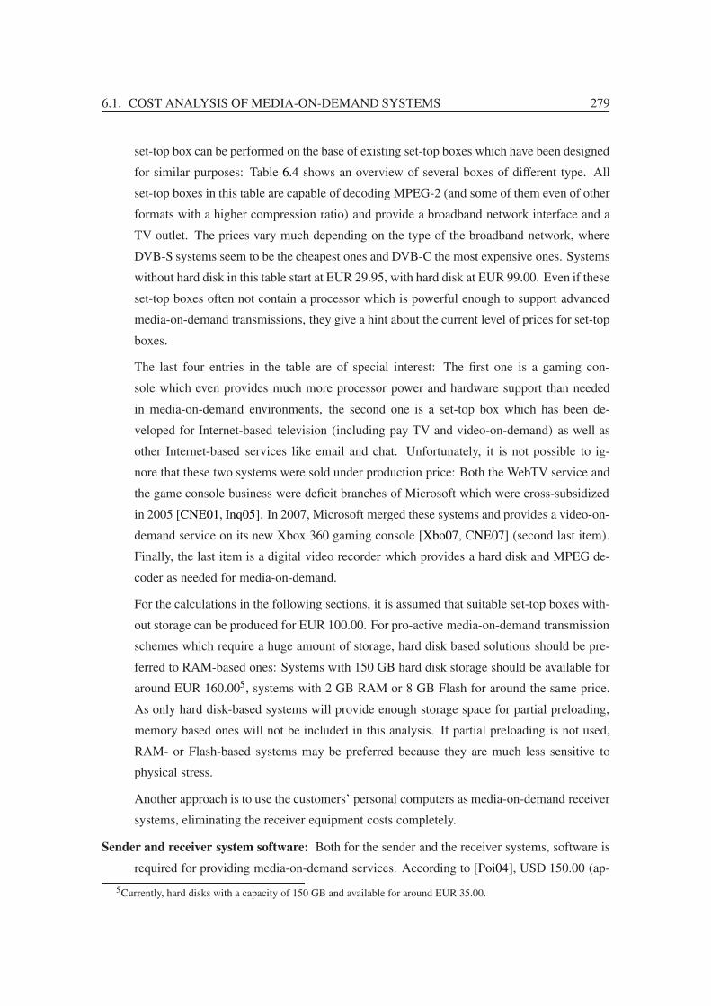
6.1. COST ANALYSIS OF MEDIA-ON-DEMAND SYSTEMS 279
set-top box can be performed on the base of existing set-top boxes which have been designed
for similar purposes: Table 6.4 shows an overview of several boxes of different type. All
set-top boxes in this table are capable of decoding MPEG-2 (and some of them even of other
formats with a higher compression ratio) and provide a broadband network interface and a
TV outlet. The prices vary much depending on the type of the broadband network, where
DVB-S systems seem to be the cheapest ones and DVB-C the most expensive ones. Systems
without hard disk in this table start at EUR 29.95, with hard disk at EUR 99.00. Even if these
set-top boxes often not contain a processor which is powerful enough to support advanced
media-on-demand transmissions, they give a hint about the current level of prices for set-top
boxes.
The last four entries in the table are of special interest: The first one is a gaming con-
sole which even provides much more processor power and hardware support than needed
in media-on-demand environments, the second one is a set-top box which has been de-
veloped for Internet-based television (including pay TV and video-on-demand) as well as
other Internet-based services like email and chat. Unfortunately, it is not possible to ig-
nore that these two systems were sold under production price: Both the WebTV service and
the game console business were deficit branches of Microsoft which were cross-subsidized
in 2005 [CNE01, Inq05]. In 2007, Microsoft merged these systems and provides a video-on-
demand service on its new Xbox 360 gaming console [Xbo07, CNE07] (second last item).
Finally, the last item is a digital video recorder which provides a hard disk and MPEG de-
coder as needed for media-on-demand.
For the calculations in the following sections, it is assumed that suitable set-top boxes with-
out storage can be produced for EUR 100.00. For pro-active media-on-demand transmission
schemes which require a huge amount of storage, hard disk based solutions should be pre-
ferred to RAM-based ones: Systems with 150 GB hard disk storage should be available for
around EUR 160.005, systems with 2 GB RAM or 8 GB Flash for around the same price.
As only hard disk-based systems will provide enough storage space for partial preloading,
memory based ones will not be included in this analysis. If partial preloading is not used,
RAM- or Flash-based systems may be preferred because they are much less sensitive to
physical stress.
Another approach is to use the customers’ personal computers as media-on-demand receiver
systems, eliminating the receiver equipment costs completely.
Sender and receiver system software: Both for the sender and the receiver systems, software is
required for providing media-on-demand services. According to [Poi04], USD 150.00 (ap-
5Currently, hard disks with a capacity of 150 GB and available for around EUR 35.00.

280 CHAPTER 6. ANALYSIS OF APPLICATION CASES
Set-top box type Brand Capabilities Price
DVB-T receiver box ComAG SL 25T Terrestrial DVB tuner, MPEG-2
decoder, TV-out
EUR 24.99
DVB-T receiver box Skymaster DVRT
1000
Terrestrial DVB tuner, MPEG-2
decoder, TV-out, 80 GB hard
disk
EUR 99.95
DVB-S receiver box Skymaster DX 15 Satellite DVB tuner, MPEG-2
decoder, TV-out
EUR 22.99
DVB-S receiver box Medion MD24500 Satellite DVB tuner, MPEG-2
decoder, TV-out, 40 GB hard
disk
EUR 99.00
DVB-C receiver box TechnoTrend micro
C202
Cable DVB tuner, MPEG-2
decoder, TV-out
EUR 59.30
DVB-C receiver box Humax PDR 9700C Cable DVB tuner, MPEG-2
decoder, TV-out, 80 GB hard
disk
EUR 248.00
Gaming console Microsoft Xbox MPEG-2 decoder, TV-out, DVD
drive, 8 GB hard disk, Ethernet
EUR 129.90 (not
sold any more)
IPTV receiver box Microsoft MSN
TV2
Windows Media 9 decoder,
wireless keyboard, USB 2.0
(e. g. for connecting a hard
disk), intended for cable,
satellite or DSL use
USD 79.00–179.00
(not sold any more)
Gaming console Microsoft
Xbox 360 Premium
System
MPEG-2 decoder, TV-out, DVD
drive, 20 GB hard disk, Ethernet
EUR 253.99
Digital video
recorder
LG Electronics
RH-256
MPEG-2 decoder, TV-out, DVD
drive, 160 GB hard disk
EUR 159.00
Table 6.4: Examples of set-top boxes of different type
proximately EUR 94.30) had been accounted for by Kingston Communications when they
set up their Point-to-Point-based media-on-demand service. In [Kuh99], the total costs for
Point-to-Point media-on-demand sender systems (hardware and software) are estimated as
USD 350.00 (approximately EUR 220.00) per receiver system which roughly acknowledges
the price estimates for hardware and software.
In case of Generalized Greedy Broadcasting media-on-demand systems, these prices dif-
fer much as the media-on-demand sender systems do not depend on the number of active
receiver systems but mainly on the number of media streams. Hence, EUR 8 000.00 are
assessed for sender software per media title and EUR 40.00 for software for each receiver
system for the Generalized Greedy Broadcasting scheme which roughly reflects personal
experiences.
To make the comparison more balanced, the software costs of Point-to-Point transmissions
are also split into a sender and a receiver system part: For receiver systems, software costs

6.1. COST ANALYSIS OF MEDIA-ON-DEMAND SYSTEMS 281
of EUR 20.00 per receiver system are assumed which should reflect that receiving a media
stream on a reactive system is less complicated than for Generalized Greedy Broadcast-
ing scheme systems. For sender systems, costs of EUR 74.00 remain per receiver system
according to the above stated total software costs which corresponds to EUR 370.00 per
concurrently active transmission if a peak usage of 20 % is assumed (which has been used
for the price estimation in [Poi04]).
For the hybrid case, the most popular media streams are sent using the Generalized Greedy
Broadcasting scheme and the remaining streams using Point-to-Point transmissions. Thus
for the sender systems, there will be both types of software present. For the receiver systems,
it is assumed that the Generalized Greedy Broadcasting receiver software is also capable to
play Point-to-Point transmissions6.
Network installation and operation: Media transmissions require a huge amount of bandwidth,
and depending on the used transmission scheme, the costs for setting up the network infras-
tructure and utilizing it for media-on-demand transmissions differ:
For small-sized environments, Ethernet equipment is very cheap today (e. g. managed
switches are available starting around EUR 6.00 per port for 100 Mbit/s and around
EUR 20.00 per port for 1 Gbit/s). In addition to the hardware, costs from installing cables
have to be considered. A study [Cis04] estimated the installation costs for CAT5 Ethernet
cables in a hotel to USD 150.00 per port.
For providing media-on-demand via DSL, the authors of [Poi04] listed capital costs of
USD 250.00 for ADSL lines and DSL access modulators per household.
For satellite-based transmissions, it is not assumed that the provider owns the network
(launching rockets with satellites is very expensive) but that satellites are leased. Unfor-
tunately, costs for satellite transmissions are very high: Leasing a transponder channel of
a satellite (with a net capacity of around 47 Mbit/s in case of DVB-S2 using 8PSK 3/5
modulation) causes annual costs between EUR 1 000 000 (which is used in this analysis)
up to EUR 6 000 000 for satellites at commonly used sky positions. Additionally, receiver
equipment for around EUR 100.00 per receiver system is required.
Media license fees: Content providers and aggregators request a license fee for distribution of
media streams. Typically, these fees are negotiated with the content providers or aggregators
which request a given percentage from the takings.
Deployment costs: For setting up a media-on-demand service, an initial huge amount of money
has to be invested: The hardware has to be installed, the service has to be promoted and
6If RTP translators are used at the receiver systems for segmented media-on-demand reception, this assumption
should be valid.

282 CHAPTER 6. ANALYSIS OF APPLICATION CASES
service employees have to be trained. In [Kuh02], the deployment costs are estimated as
USD 300 000.00 (approximately EUR 188 000.00) for a large environment installation, but
smaller installations should be much cheaper.
Operational expenses: To maintain the system and to supply required resources as well as man-
aging customers and company needs, several additional costs have to be considered (e. g.
room rental, electric power supply, telephone support for customers, billing of customers,
promotion, accounting). These expenses seem to vary much depending on the operator:
According to [Kuh99], these expenses have averaged USD 4.00 and are still falling. Some
companies already reached USD 1.20 per month and subscriber in year 1999 which is the
latest reliable statement.
Capital recovery: As media-on-demand providers like to get their investments returned after
some time, a recovery time for the capital costs has to be defined. According to [Poi04], a
capital recovery after five years is typical in this class of business.
To compare the two different transmission techniques, only hardware and software costs and
for satellite-based environments network costs are relevant. Table 6.5 summarizes these costs in a
table.
Sender systems:
EUR 126.00 per active rcv. for Point-to-Point transmissions
EUR 630.00 per title for Generalized Greedy Broadcasting
transmissions
Receiver systems:
EUR 100.00 per receiver for Point-to-Point transmissions
EUR 160.00 per receiver for Generalized Greedy Broadcasting
transmissions
Sender software:
EUR 370.00 per active rcv. for Point-to-Point transmissions
EUR 8000.00 per title for Generalized Greedy Broadcasting
transmissions
Receiver software:
EUR 20.00 per receiver for Point-to-Point transmissions
EUR 40.00 per receiver for Generalized Greedy Broadcasting
transmissions
Network bandwidth:
EUR 1000000.00 per transp. and year for satellite-based environments
Table 6.5: Overview of costs which depend on the used transmission technique
Revenue from Media-on-Demand
The following sources of revenue from media-on-demand services can be opposed to the above
described costs:

6.2. EVALUATION IN ETHERNET-BASED ENVIRONMENTS 283
Revenue from rental or selling of receiver system equipment: If a receiver system equipment
is required (i. e. if not an existing system such as a personal computer is used), the provider
may rent or sell receiver systems to its customers. On the other hand, it is also possible to
subsidize the equipment in order to push the service.
In this analysis, the media-on-demand receiver system costs are allocated completely to the
monthly fees, based on a capital recovery of five years.
Pay-per-view charges or periodical customer fees: For using the media-on-demand service,
the provider may charge a periodical fee from the customer and/or a rate per received media-
stream. Typical prices range from below EUR 1.00 for filmlets or TV episodes up to around
EUR 2.50–4.00 for new titles (e. g. for T-Online videoload, Comcast pay-per-view or Mi-
crosofts IPTV services).
Setup and registration fees: Initial setup fees are very uncommon for media-on-demand. In
cases where costs are caused from the receiver system equipment or the installation of the
broadband network access, these costs are typically allocated to monthly fees.
Advertising revenue: Similar to private television broadcasting, advertisements can be used to
cover some of the expenses of the media-on-demand service. But depending on the local
habits, advertising for a paid service may not be accepted by customers.
A possible solution would be a twofold offer which allows the customer to choose between
a cheap, advertisement sponsored transmission and a more expensive transmission without
any commercial breaks.
Besides these, several indirect benefits may be achieved (e. g. increase of the company image
and value). As none of these benefits depend much on the used transmission technique, they are
ignored in the comparison.
6.2 Evaluation of Media-on-Demand in Ethernet-Based Environ-
ments
For small environments, high bandwidth networks are typically available for relatively low costs:
Switched Ethernet excellently fulfills the requirements for both Point-to-Point media-on-demand
transmissions and transmissions using a pro-active scheme like the Generalized Greedy Broadcast-
ing scheme. Thus the efficiency of the transmission scheme plays only a minor role, the evaluation
is mainly influenced by the costs of the sender and receiver system equipment and software.
Consequently, this has a major impact on the cost-effectiveness of the different media-on-
demand system approaches: The following two subsections present a sample calculation for

284 CHAPTER 6. ANALYSIS OF APPLICATION CASES
a small, Ethernet-based media-on-demand system for both of the two examined transmission
schemes.
6.2.1 Point-to-Point Transmissions
This setup allows to use the cheap, storage-free receiver systems, thus the transmission technique-
dependent costs are moderately low as shown in table 6.6. If the customers’ personal computer sys-
tems are used as media-on-demand receiver systems, the costs can be lowered by EUR 20 000.00
(EUR 100.00 per receiver).
Item Costs Total
Sender systems (PtP) EUR 126.00 per active rcv. EUR 20160.00
Receiver systems (PtP) EUR 100.00 per receiver EUR 20000.00
Sender software (PtP) EUR 370.00 per active rcv. EUR 59200.00
Receiver software (PtP) EUR 20.00 per receiver EUR 4000.00
Costs EUR 516.80 per customer EUR 103360.00
Table 6.6: Transmission technique-dependent costs for Ethernet-based Point-to-Point transmis-
sions
6.2.2 Generalized Greedy Broadcasting Transmissions
This setup requires the use of set-top boxes which are capable of storing part of the media stream.
For hard disk-based set-top boxes, the transmission technique-dependent costs are shown in ta-
ble 6.7 for a media assortment of 20 titles. Results for media assortments of other size are shown
in table 6.8. Other choices in the examined setups (e. g. playback delay and amount of preload-
ing for Generalized Greedy Broadcasting scheme) do not influence the results in this environment
because the used network costs are very low and cannot be reduced this way. If the customers’ per-
sonal computer systems are used as media-on-demand receiver systems, the costs can be lowered
in this setup by EUR 32 000.00 (EUR 160.00 per receiver).
Item Costs Total
Sender systems (GGB) EUR 630.00 per title EUR 12600.00
Receiver systems (GGB) EUR 160.00 per receiver EUR 32000.00
Sender software (GGB) EUR 8000.00 per title EUR 160000.00
Receiver software (GGB) EUR 20.00 per receiver EUR 8000.00
Costs EUR 1063.00 per customer EUR 212600.00
Table 6.7: Transmission technique-dependent costs for Ethernet-based Generalized Greedy Broad-
casting transmissions

6.2. EVALUATION IN ETHERNET-BASED ENVIRONMENTS 285
Size of Costs Costs
assortment (per customer) (total)
10 EUR 631.50 EUR 126300.00
20 EUR 1063.00 EUR 212600.00
50 EUR 2357.50 EUR 471500.00
100 EUR 4515.00 EUR 903000.00
Table 6.8: Transmission technique-dependent costs for Ethernet-based Generalized Greedy Broad-
casting transmissions assuming different media assortment sizes
6.2.3 Hybrid Setup
In the hybrid setup, the receiver systems must be capable to receive a media stream using the Gen-
eralized Greedy Broadcasting scheme, so the receiver systems will be the same as in the previous
setup. For the sender systems, a balance between Point-to-Point transmissions and Generalized
Greedy Broadcasting transmissions must be found: For the presumed sender system and sender
software costs, the Generalized Greedy Broadcasting scheme is more advantageous than separate
Point-to-Point transmissions for titles with at least 18 active receivers. Assuming the Zipf distri-
bution for the popularity of the titles, this is only the case for the most popular two titles in case of
a medium assortment of 20 titles. Table 6.9 shows the composition of the costs for this setup and
table 6.10 the results for different assortment sizes.
Item Costs Total
Sender systems (PtP) EUR 126.00 per active rcv. EUR 13986.00
Sender systems (GGB) EUR 630.00 per title EUR 1260.00
Receiver systems (hybrid) EUR 160.00 per receiver EUR 32000.00
Sender software (PtP) EUR 370.00 per active rcv. EUR 41070.00
Sender software (GGB) EUR 8000.00 per title EUR 16000.00
Receiver software (hybrid) EUR 20.00 per receiver EUR 8000.00
Costs EUR 561.58 per customer EUR 112316.00
Table 6.9: Transmission technique-dependent costs for Ethernet-based hybrid Point-to-
Point/Generalized Greedy Broadcasting setups
Size of Titles Active rcv. Costs Costs
assortment PtP/GGB PtP/GGB (per customer) (total)
10 7/3 75/85 EUR 515.45 EUR 103090.00
20 18/2 111/49 EUR 561.58 EUR 112316.00
50 49/1 139/21 EUR 587.87 EUR 117574.00
100 100/0 160/0 EUR 596.80 EUR 119360.00
Table 6.10: Transmission technique-dependent costs for Ethernet-based hybrid Point-to-
Point/Generalized Greedy Broadcasting setups assuming different media assortment sizes

286 CHAPTER 6. ANALYSIS OF APPLICATION CASES
6.2.4 Result
For Ethernet-based, small environments, Point-to-Point media-on-demand systems are signifi-
cantly less expensive than Generalized Greedy Broadcasting transmissions as shown in figure 6.2.
Even a hybrid setup of Generalized Greedy Broadcasting for the most popular titles and Point-to-
Point transmissions for the remaining ones is more expensive than a pure Point-to-Point streaming
setup. The main reason for this is that there are too few recipients for the same media title to com-
pensate for the higher costs caused by Generalized Greedy Broadcasting for systems and software.
Only if the media assortment is very small (consisting of up to seven streams for a General-
ized Greedy Broadcasting setup or up to ten streams for a hybrid setup), the Generalized Greedy
Broadcasting scheme provides lower costs: If only very few media streams are sent, the lower
sender system costs for the Generalized Greedy Broadcasting scheme compensate for the higher
receiver system costs.
300
400
500
600
700
800
900
1000
10 20 30 40 50 60 70 80 90 100
Co
sts
Size of Media Assortment
Costs for Generalized Greedy Broadcasting TransmissionsCosts for Hybrid Setup
Costs for Point-to-Point Transmissions
Figure 6.2: Transmission technique-dependent costs for Ethernet-based setups in relation to the
media assortment size
6.3 Evaluation of Media-on-Demand in DSL-Based Environments
In environments where customers already have DSL-based Internet access, media-on-demand ser-
vices can be provided in a very simple way. With the enormous spread of DSL-based Internet
accesses, this type of media-on-demand has become very popular in recent years, nearly each
Internet service provider offers a video-on-demand service.

6.3. EVALUATION IN DSL-BASED ENVIRONMENTS 287
The bandwidth requirements of Point-to-Point media-on-demand transmissions are around
2.178 Mbit/s for each active transmission which can be accomplished in many cases where DSL
is available if only one media stream per DSL line is consumed concurrently. If pro-active media-
on-demand transmission schemes should be used, the bandwidth requirements are much higher
because several channels have to be received at once (e. g. up to 10.52 Mbit/s for the examined
setups, see table 6.3). Although 6 Mbit/s DSL is often supported and even higher rates are in
preparation7, these bandwidths may not be achievable for all customers. Fortunately, the General-
ized Greedy Broadcasting scheme can support the case that less bandwidth is available:
• The Generalized Greedy Broadcasting scheme provides support for limited receiver band-
width (see section 4.18) which makes it possible to transmit the media stream in such a way
that only a fraction of the channels has to be joined at a time.
• The Generalized Greedy Broadcasting scheme supports channels of arbitrary bandwidth
(see section 4.10) which allows to select the bandwidth of channels independent from the
media stream bit rate.
• The Generalized Greedy Broadcasting scheme supports layered encodings (see section 5.2)
so poorly connected receiver systems can receive media streams at reduced quality.
Using these enhancements, it is even possible to send a 2.178 Mbit/s media stream with the Gen-
eralized Greedy Broadcasting scheme on 3 Mbit/s or 6 Mbit/s DSL lines in full quality or at lower
bit rates in reduced quality.
The disadvantage of a low receiver bandwidth is that the sender bandwidth is increased: For
example, the sender bandwidth for media-on-demand transmissions with a playback delay of 1120
of the media stream duration and no preloading is increased from 10.52 Mbit/s to 17.69 Mbit/s if
the receiver bandwidth is limited to 3 Mbit/s and to 11.32 Mbit/s if limited to 6 Mbit/s. As this only
increases the network consumption at the DSL access concentrator where the media-on-demand
traffic is routed to the DSL lines, this increase is negligible.
The costs for the two media-on-demand transmission schemes compare as follows:
6.3.1 Point-to-Point Transmissions
As for the Ethernet-based environment, this setup allows to use the less expensive, storage-free
receiver systems. Table 6.11 shows the transmission technique-dependent costs in this case.
If the customers’ personal computer systems are used as media-on-demand receiver systems in
this setup (which is very probably because they may be connected to the Internet via DSL either),
costs can be lowered by EUR 2 000 000.00 (EUR 100.00 per receiver).
7Deutsche Telecom has installed VDSL2 Internet access in the 50 hugest German cities until 2007, providing up to
50 Mbit/s using outdoor DSL access modulators to shorten the distance to the next access modulator.
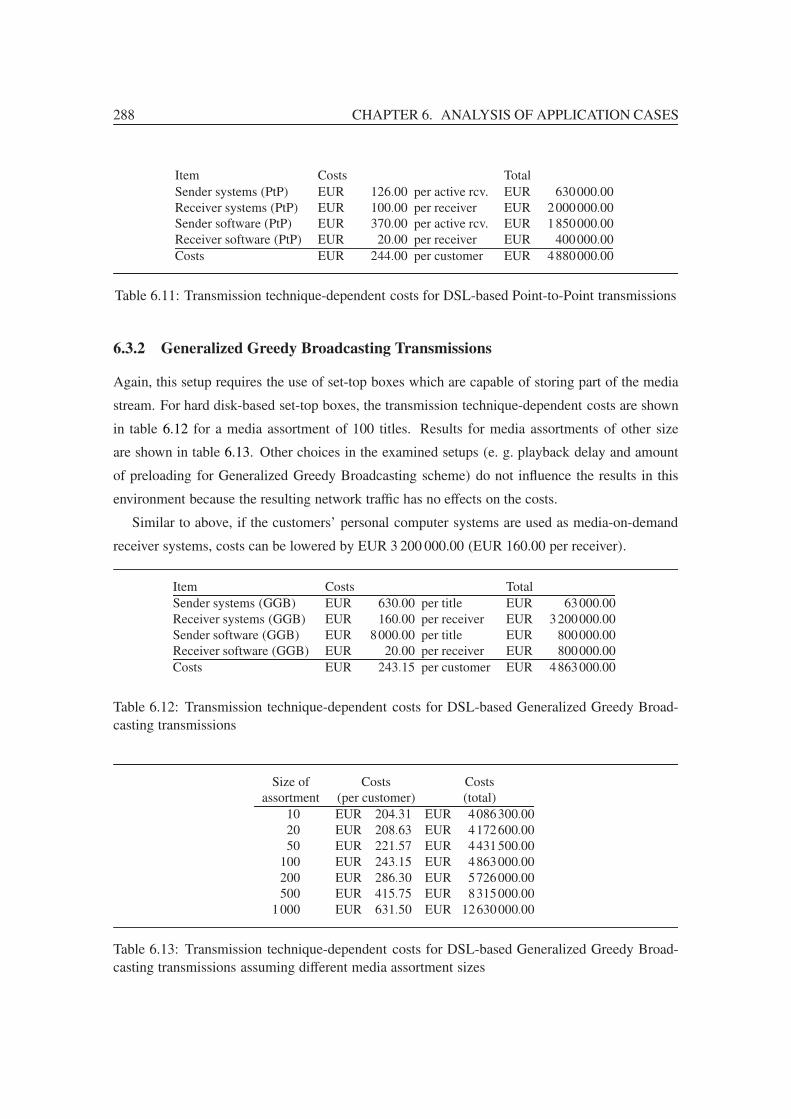
288 CHAPTER 6. ANALYSIS OF APPLICATION CASES
Item Costs Total
Sender systems (PtP) EUR 126.00 per active rcv. EUR 630000.00
Receiver systems (PtP) EUR 100.00 per receiver EUR 2000000.00
Sender software (PtP) EUR 370.00 per active rcv. EUR 1850000.00
Receiver software (PtP) EUR 20.00 per receiver EUR 400000.00
Costs EUR 244.00 per customer EUR 4880000.00
Table 6.11: Transmission technique-dependent costs for DSL-based Point-to-Point transmissions
6.3.2 Generalized Greedy Broadcasting Transmissions
Again, this setup requires the use of set-top boxes which are capable of storing part of the media
stream. For hard disk-based set-top boxes, the transmission technique-dependent costs are shown
in table 6.12 for a media assortment of 100 titles. Results for media assortments of other size
are shown in table 6.13. Other choices in the examined setups (e. g. playback delay and amount
of preloading for Generalized Greedy Broadcasting scheme) do not influence the results in this
environment because the resulting network traffic has no effects on the costs.
Similar to above, if the customers’ personal computer systems are used as media-on-demand
receiver systems, costs can be lowered by EUR 3 200 000.00 (EUR 160.00 per receiver).
Item Costs Total
Sender systems (GGB) EUR 630.00 per title EUR 63000.00
Receiver systems (GGB) EUR 160.00 per receiver EUR 3200000.00
Sender software (GGB) EUR 8000.00 per title EUR 800000.00
Receiver software (GGB) EUR 20.00 per receiver EUR 800000.00
Costs EUR 243.15 per customer EUR 4863000.00
Table 6.12: Transmission technique-dependent costs for DSL-based Generalized Greedy Broad-
casting transmissions
Size of Costs Costs
assortment (per customer) (total)
10 EUR 204.31 EUR 4086300.00
20 EUR 208.63 EUR 4172600.00
50 EUR 221.57 EUR 4431500.00
100 EUR 243.15 EUR 4863000.00
200 EUR 286.30 EUR 5726000.00
500 EUR 415.75 EUR 8315000.00
1000 EUR 631.50 EUR 12630000.00
Table 6.13: Transmission technique-dependent costs for DSL-based Generalized Greedy Broad-
casting transmissions assuming different media assortment sizes

6.3. EVALUATION IN DSL-BASED ENVIRONMENTS 289
6.3.3 Hybrid Setup
As the sender system costs for this setup are the same as for the Ethernet-based setup, a Gener-
alized Greedy Broadcasting causes lower costs for titles with at least 18 active receivers. But as
a much higher number of receivers is assumed in this setup, this number is reached for 99 of the
100 titles.
To give a more practical example for a DSL-based hybrid setup, the size of the media assort-
ment is increased to 200 titles. In this case, the 71 most popular titles (which receive around
69 % of all media requests) have enough active receivers to be transmitted using the Generalized
Greedy Broadcasting scheme. The resulting transmission technique-dependent costs for this setup
are shown in table 6.14 and for other media assortments in table 6.15.
Item Costs Total
Sender systems (PtP) EUR 126.00 per active rcv. EUR 192402.00
Sender systems (GGB) EUR 630.00 per title EUR 44730.00
Receiver systems (hybrid) EUR 160.00 per receiver EUR 3200000.00
Sender software (PtP) EUR 370.00 per active rcv. EUR 564990.00
Sender software (GGB) EUR 8000.00 per title EUR 568000.00
Receiver software (hybrid) EUR 20.00 per receiver EUR 800000.00
Costs EUR 268.51 per customer EUR 5370122.00
Table 6.14: Transmission technique-dependent costs for DSL-based hybrid Point-to-
Point/Generalized Greedy Broadcasting setups
Size of Titles Active rcv. Costs Costs
assortment PtP/GGB PtP/GGB (per customer) (total)
10 0/10 0/5 000 EUR 204.31 EUR 4086300.00
20 0/20 0/5 000 EUR 208.63 EUR 4172600.00
50 0/50 0/5 000 EUR 221.57 EUR 4431500.00
100 1/99 17/4 983 EUR 243.14 EUR 4862802.00
200 129/71 1 527/3 473 EUR 268.51 EUR 5370122.00
500 453/47 2 800/2 200 EUR 289.72 EUR 5794410.00
1000 966/34 3 442/1 558 EUR 300.03 EUR 6000652.00
Table 6.15: Transmission technique-dependent costs for DSL-based hybrid Point-to-
Point/Generalized Greedy Broadcasting setups assuming different media assortment sizes
6.3.4 Results
For the preconditions of the DSL-based setup, media-on-demand using Point-to-Point transmis-
sions and the Generalized Greedy Broadcasting scheme cause nearly identical costs. Although
the receiver systems are more expensive for media-on-demand based on pro-active schemes, the

290 CHAPTER 6. ANALYSIS OF APPLICATION CASES
Generalized Greedy Broadcasting scheme has lower costs for sender systems. Graph 6.3 shows
this for different sizes of media assortments.
200
220
240
260
280
300
320
340
0 100 200 300 400 500 600 700 800 900 1000
Co
sts
Size of Media Assortment
Costs for Generalized Greedy Broadcasting TransmissionsCosts for Hybrid Setup
Costs for Point-to-Point Transmissions
Figure 6.3: Transmission technique-dependent costs for DSL-based setups in relation to the media
assortment size
For media assortments with 102 titles or more, the costs of the receiver systems overweigh the
savings in the sender systems, so Point-to-Point transmissions are less expensive. But with a grow-
ing number of receiver systems, this boundary moves in favor of the Generalized Greedy Broad-
casting scheme: For a setup ten times the size of the medium sized setup (so 200 000 recipients
and a maximum of 50 000 concurrently active receivers), the Generalized Greedy Broadcasting
scheme performs at lower costs for all titles of a media assortment with 1 000 titles as shown in
figure 6.4.
6.4 Evaluation of Media-on-Demand in Satellite-Based Environ-
ments
Satellite-based networks can be used to access a very large number of customers at once. As band-
width of satellites is highly valuable, it must not be wasted, thus the efficiency of the transmission
scheme gains highest importance. Therefore, it is nearly obvious that Point-to-Point transmissions
are ineffective in this setup:

6.4. EVALUATION IN SATELLITE-BASED ENVIRONMENTS 291
200
220
240
260
280
300
0 100 200 300 400 500 600 700 800 900 1000
Co
sts
Size of Media Assortment
Costs for Point-to-Point TransmissionsCosts for Generalized Greedy Broadcasting Transmissions
Costs for Hybrid Setup
Figure 6.4: Transmission technique-dependent costs for a larger DSL-based setup in relation to
the media assortment size
6.4.1 Point-to-Point Transmissions
Table 6.16 shows the transmission technique-dependent costs for the satellite-based environment.
The costs are much lower than for the smaller setups because for a lower number of concurrently
active receiver systems has been assumed.
Item Costs Total
Sender systems (PtP) EUR 126.00 per active rcv. EUR 63000000.00
Receiver systems (PtP) EUR 100.00 per receiver EUR 200000000.00
Sender software (PtP) EUR 370.00 per active rcv. EUR 185000000.00
Receiver software (PtP) EUR 20.00 per receiver EUR 40000000.00
Costs EUR 244.00 per customer EUR 488000000.00
Table 6.16: Transmission technique-dependent costs for satellite-based Point-to-Point transmis-
sions
In addition to these costs, satellite bandwidth has to be leased, but serving 500 000 concur-
rently active receivers using Point-to-Point transmissions would require a bandwidth of more than
1 Tbit/s! Besides of the incomprehensible sum for leasing this amount of satellite bandwidth
(more than EUR 20 000 000 000 per year according to the prerequisites), this would allocate the
total bandwidth of 465 satellites (assuming 50 transponders per satellite), making this scenario
pure theory.

292 CHAPTER 6. ANALYSIS OF APPLICATION CASES
6.4.2 Generalized Greedy Broadcasting Transmissions
While the system costs of the this case do not differ much from the Point-to-Point case (see ta-
ble 6.17 and 6.18), the bandwidth costs are much lower: Broadcasting 200 titles with a varying
playback delay between immediate service and d60
depending on media popularity and utilizing d12
of preloading requires a total bandwidth of 1.02 Gbit/s. This equals nearly 23 transponders, thus
EUR 23 000 000 per year or EUR 0.96 per month and customer which is more realistic. Results
for other combinations of playback delay, preloading and size of media assortment are given in
table 6.19.
Item Costs Total
Sender systems (GGB) EUR 630.00 per title EUR 126000.00
Receiver systems (GGB) EUR 160.00 per receiver EUR 320000000.00
Sender software (GGB) EUR 8000.00 per title EUR 1600000.00
Receiver software (GGB) EUR 20.00 per receiver EUR 80000000.00
Costs EUR 200.86 per customer EUR 401726000.00
Table 6.17: Transmission technique-dependent costs for satellite-based Generalized Greedy
Broadcasting transmissions
Size of Costs Costs
assortment (per customer) (total)
10 EUR 200.04 EUR 400086300.00
20 EUR 200.09 EUR 400172600.00
50 EUR 200.22 EUR 400431500.00
100 EUR 200.43 EUR 400863000.00
200 EUR 200.86 EUR 401726000.00
500 EUR 202.16 EUR 404315000.00
1000 EUR 204.31 EUR 408630000.00
Table 6.18: Transmission technique-dependent costs for satellite-based Generalized Greedy
Broadcasting transmissions assuming different media assortment sizes
6.4.3 Hybrid Setup
The hybrid setup has no advantages to Generalized Greedy Broadcasting transmissions in a large
environment: Due to the high number of active recipients, all titles are requested by enough active
receiver systems to give the Generalized Greedy Broadcasting scheme the advantage.

6.5. CONCLUSION 293
Playback Amount of No. of No. of Operational costs Operational costs
delay preloading titles transp. (per customer) (total)
0 d60
200 40 EUR 1.67 EUR 3333333.33
0 d12
200 25 EUR 1.04 EUR 2083333.33d
1200 200 50 EUR 2.08 EUR 4166666.67
d120
d60
200 40 EUR 1.67 EUR 3333333.33d
120d12
200 25 EUR 1.04 EUR 2083333.33d60
0 200 40 EUR 1.67 EUR 3333333.33d60
d60
200 34 EUR 1.42 EUR 2833333.33d60
d12
200 23 EUR 0.96 EUR 1916666.67
varying d60
200 34 EUR 1.42 EUR 2833333.33
varying d12
200 23 EUR 0.96 EUR 1916666.67
0 d60
50 10 EUR 0.42 EUR 833333.33
0 d12
50 7 EUR 0.29 EUR 583333.33d
1200 50 13 EUR 0.54 EUR 1083333.33
d120
d60
50 10 EUR 0.42 EUR 833333.33d
120d12
50 7 EUR 0.29 EUR 583333.33d60
0 50 10 EUR 0.42 EUR 833333.33d60
d60
50 9 EUR 0.38 EUR 750000.00d60
d12
50 6 EUR 0.25 EUR 500000.00
varying d60
50 9 EUR 0.38 EUR 750000.00
varying d12
50 6 EUR 0.25 EUR 500000.00
0 d60
10 2 EUR 0.08 EUR 166666.67
0 d12
10 2 EUR 0.08 EUR 166666.67d
1200 10 3 EUR 0.12 EUR 250000.00
d120
d60
10 2 EUR 0.08 EUR 166666.67d
120d12
10 2 EUR 0.08 EUR 166666.67d60
0 10 2 EUR 0.08 EUR 166666.67d60
d60
10 2 EUR 0.08 EUR 166666.67d60
d12
10 2 EUR 0.08 EUR 166666.67
varying d60
10 2 EUR 0.08 EUR 166666.67
varying d12
10 2 EUR 0.08 EUR 166666.67
Table 6.19: Monthly bandwidth costs for satellite-based Generalized Greedy Broadcasting trans-
missions using different transmission parameters
6.4.4 Results
As expected, the analysis shows that Point-to-Point transmissions cannot be used efficiently for
media-on-demand via satellite. Nevertheless, due to the high costs of satellite bandwidth, regular
monthly costs occur which require a high number of customers to be cost-effective.
6.5 Conclusion
In this chapter, two media-on-demand system approaches have been analyzed from a financial
point of view: Firstly, a media-on-demand system which is based on Point-to-Point transmissions
which is the commonly used type of system today, and secondly, a system based on the General-

294 CHAPTER 6. ANALYSIS OF APPLICATION CASES
ized Greedy Broadcasting scheme which has been proposed and evaluated in the previous chapters
as a highly efficient and flexible solution for pro-active media-on-demand services.
This analysis proved for the assumed preconditions that the pro-active approach of the Gener-
alized Greedy Broadcasting scheme evolved to be equivalent to Point-to-Point based systems in
medium-sized environments and superior in large environments, in satellite based environments as
well as in setups where the receiver systems are connected via DSL to media-on-demand sender
systems. This is especially interesting as DSL-based media-on-demand services using Point-to-
Point transmission schemes have spread much in recent years.
For small, Ethernet-based environments, Point-to-Point media-on-demand systems are the less
expensive alternative because of higher software and hardware costs of Generalized Greedy trans-
missions. But even in these environments Generalized Greedy based systems are more cost-
effective if the media assortment is very small.
Altogether, this chapter evolved that Generalized Greedy Broadcasting transmissions can sub-
stitute Point-to-Point transmissions because of lower costs and better scalability in many applica-
tion cases.

Chapter 7
Conclusion
IN this thesis, media-on-demand systems have been examined and enhanced, both in theory and
from practical points of view. To summarize the attained results, the achievements are reviewed
briefly in this final chapter: Section 7.1 covers conceptual achievements which have been reached
and sections 7.2 and 7.3 detail improvements of efficiency and utilizability. Finally, in the last
section of this chapter, the future trend of media-on-demand is described from the author’s point
of view.
7.1 Conceptual Achievements
To understand the functioning of media-on-demand systems, chapter 2 started with a dissection of
media-on-demand systems into functional components. Besides the knowledge gained from the
detailed examination as a result of the decomposition itself, this decomposition revealed different
aspects of media-on-demand systems which can be improved:
At a first level of dissection, the overall structure of media-on-demand systems can be en-
hanced. Therefore, the author of this thesis introduced hierarchical media-on-demand systems:
In a hierarchical media-on-demand system, several sender systems are organized in a tree-like or
mesh-like structure, forwarding media streams downwards the tree hierarchy or between sender
systems in a mesh. This eliminates the need to explicitely distribute media streams to all sender
systems, the whole setup works like one huge, distributed media-on-demand system. Addition-
ally, the storage requirements of most of the sender systems are lowered because these systems do
not have to store all media stream permanently: When a media stream is requested from a sender
system which is not in its storage, it can request a media-on-demand transmission for the media
stream from another sender system and forward the data to the receiver system.
A deeper look at the structure of media-on-demand systems disclosed that media-on-demand
transmissions are driven by a transmission scheme: The transmission scheme defines how media

296 CHAPTER 7. CONCLUSION
streams are transmitted from sender to receiver systems. Therefore the author of this thesis pre-
sented a classification and detailed analysis of functioning, advantages and drawbacks of a wide
range of transmission schemes in chapter 3.
This examination showed that the schemes can be divided into several groups: Reactive trans-
mission schemes, which schedule transmissions based on requests from receiver systems, pro-
active transmission schemes which perform permanent transmissions independent of requests from
receiver systems and reactive-pro-active hybrids which combine approaches of both variants.
While reactive transmission schemes perform very well if media streams are only requested by
few receiver systems, they do not scale for large environments with lots of receiver systems. In
contrast, the functioning of pro-active systems is independent of the number of active receiver sys-
tems, but as they perform transmissions permanently, they even consume resources if no receiver
system is listening to the transmission. Combining these approaches into hybrid systems allows
to benefit from both variants, scalability for large environments and economic use of resources for
cases with few active receivers.
Besides this grouping of transmission schemes based on the functioning of their scheduling
algorithm, the author rated all examined transmission schemes using several technical and func-
tional classifications, e. g. for the supported playback controls (pause, rewind, fast-forward) and
the ability to perform live transmissions.
7.2 Efficiency Improvements
Besides the functioning and capabilities of media-on-demand transmission schemes, the resource
requirements for media-on-demand are important, esp. the bandwidth requirements of the sender
system, the bandwidth requirements of receiver systems and the amount of needed storage at
receiver systems.
For the analysis of the sender system bandwidth requirements, the author of this thesis intro-
duced a measure: the efficiency of the media-on-demand transmission scheme. The efficiency of
a transmission scheme quantifies how much bandwidth a transmission scheme uses compared to
the amount of bandwidth which is absolutely needed from an information theoretic point of view.
One side-effect of this definition for efficiency is that it is independent of the media bit rate,
thus the media-on-demand transmission schemes can be rated independent of the media encoding.
Nevertheless, as the media bit rate influences the bandwidth requirements of sender and receiver
systems, advanced media compression algorithms have been recommended, allowing to lower the
bandwidth requirements without a perceivable loss of media quality.
To compare the bandwidth requirements of the presented transmission schemes, the author of
this thesis analyzed the efficiency of the transmission schemes which have been presented and
classified in chapter 3. Because of the huge number of pro-active transmissions schemes, the

7.2. EFFICIENCY IMPROVEMENTS 297
author divided the group of pro-active media-on-demand transmission schemes (including the
pro-active part of hybrid schemes) further into four subgroups by the way how they transmit the
media stream:
For the first subgroup, the non-segmenting schemes, the media stream is sent linearly as a
whole. Schemes of this subgroup have a very low efficiency and are almost only of historic interest.
For schemes of the second subgroup, the size-based transmission schemes, the media stream
is split into segments of increasing size which are transmitted round-robin on separate channels
of equal bandwidth. This subgroup showed much better results, but as the analysis of the author
revealed, they cannot perform as good as the schemes of the remaining two subgroups.
The third subgroup is of special interest because it contains the transmission schemes with
the highest efficiency, even schemes which operate at an efficiency of 100 %: The bandwidth-
based transmission schemes of this subgroup perform media-on-demand transmissions by splitting
the media stream into segments of equal size and transmitting the segments on channels with
decreasing bandwidth. Unfortunately, the schemes of this subgroup have several fundamental
drawbacks which render them mostly unusable in a practical system.
Transmission schemes of the last subgroup, the frequency-based schemes, split the media-
stream into segments of equal size, too, but transmit these segments on channels of equal band-
width at decreasing frequency. Determining the period and phase shift for each segment in such a
way that they can be sent on the lowest number of channels is one of the major challanges of the
frequency-based transmission schemes: As it has been shown that finding the optimal solution is
NP-hard, simple static mappings and heuristic algorithms of different type are used for frequency-
based schemes. Unfortunately, the author found no transmission scheme of the frequency-based
subgroup, which has an efficiency nearly as high as the bandwidth-based schemes.
As a result of the gained insights from the efficiency comparison and because of the lack of
a transmision scheme which provides a high efficiency and does not suffer from the problems
of the bandwidth-based subgroup, the author of this thesis proposed a new transmission scheme
in chapter 4, the Generalized Greedy Broadcasting scheme: Using one of the frequency-based
transmission schemes as a starting point, the author generalized it and enhanced its heuristic,
thereby reaching an efficiency of more than 99 %.
In addition to reaching a high efficiency, the author of this thesis applied several mechanisms to
the Generalized Greedy Broadcasting scheme which allow to lower the sender system bandwidth
requirements independent of the efficiency (e. g. preloading the beginning of media streams to
receiver systems or utilizing planned breaks in the stream transmission to lower the transmission
bandwidth).
Last but not least, the author also extended the Generalized Greedy Broadcasting scheme in
such a way that it is able to cope with limitations of receiver systems: For receiver systems with

298 CHAPTER 7. CONCLUSION
limited bandwidth or storage, the algorithm has been adjusted to produce a schedule which respects
these limitations. Although this increases the bandwidth requirements of the sender system, the
Generalized Greedy Broadcasting scheme still operates at the same high efficiency if the receiver
system limits are considered in the efficiency calculation.
7.3 Extended Utilizability
Apart from a high efficiency, the utilizability of media-on-demand in general and of the proposed
Generalized Greedy Broadcasting scheme in particular has been extended throughout this thesis
in several directions.
Therefore, the author of this thesis first identified and analyzed the extensions which have been
presented for the transmission schemes in chapter 3. As it emerged, many transmission schemes
have been extended in some way to fit a special purpose, but no transmission scheme has been
found which supported many of the extensions at once.
As a second step, the author of this thesis extended this list by additional requirements of
consumers and providers to improve the utilizability of enhanced media-on-demand systems in
many use-cases. Altogether, this complete list included mechanisms to enhance the service for the
consumer (e. g. support for immediate playback for pro-active transmission schemes), to extend
its applicability (e. g. for live transmissions or variable-bit-rate media streams) and to support
efficient use in changing environments (e. g. replacement of media streams or change of media
stream transmission parameters in a running system). Due to the preliminary work on efficiency
analysis presented in chapter 3, the author was able to perform a detailed study of the impacts to
efficiency of each of these extensions.
Next, the author incorporated most of the found extensions into the Generalized Greedy Broad-
casting scheme in chapter 4. Thereby, the flexibility and customizability of the Generalized Greedy
Broadcasting scheme helped to integrate them in such a way that the efficiency of the Generalized
Greedy Broadcasting scheme stayed as high as ever.
Furthermore, many transport level improvements for media-on-demand systems have been pro-
posed in chapter 5 which can be applied to further increase the utilizability. For this purpose,
the author examined the availability and usability of different transport enhancement techniques
like error correction, layered media streams and security for media-on-demand. Using the stan-
dardized, widely-used Real-time Transport Protocol (RTP) together with the Session Description
Protocol (SDP) for enhanced media-on-demand transmissions and suggesting a solution for the
migration from existing media-on-demand systems to enhanced ones took another important part
in this chapter.
Finally, the author provided a comparison of the transmission technique specific costs in chap-
ter 6, comparing the utilizability of the Generalized Greedy Broadcasting scheme with traditional

7.4. FUTURE OF MEDIA-ON-DEMAND 299
point-to-point transmissions from a financial point of view. This comparison revealed that the
Generalized Greedy Broadcasting scheme is comparable with point-to-point transmission based
systems in the examined medium-sized use-case and superior for the large setup.
7.4 Future of Media-on-Demand
Some years ago, when the author started his research on media-on-demand, it was obvious that
media-on-demand was not cost-effective yet: The bandwidth requirements were very high, high
bandwidth network access was very expensive, the hardware requirements for sender and receiver
systems called for huge expenses and the distribution rights for media streams were unclear.
Nevertheless, it was predictable that this would change in near future. And as of today, the state
of affairs has changed: The bandwidth requirements have been lowered, many households have a
broadband network connection which can be used for media-on-demand services, hardware prices
have fallen steadily and content providers started to agree into distribution licenses for on-demand
services.
As a result, many major companies have entered the media-on-demand business. But unfor-
tunately, most of the used systems are based on point-to-point transmissions. Besides missing
publicity of enhanced media-on-demand transmission techniques, one of the reasons may be that
the enhanced techniques bear more risks than the simple systems for providers: As the receiver
systems for enhanced media-on-demand systems are more expensive (as they must be equipped
with storage), enhanced transmissions are only profitable if the lower sender system costs compen-
sate for this. This gives point-to-point based systems an advantage in the beginning phase where
the sender system costs are roughly proportional to the number of customers for point-to-point
based systems but proportional to the number of offered media titles for enhanced systems.
But although point-to-point transmission based systems may satisfy the current demands and
are less expensive for small systems, it is risky not to investigate into new media-on-demand
techniques: Many market analyses project an increase in media-on-demand in the next years and
it may even be possible that media-on-demand becomes an established service besides traditional
media broadcasting in near future.
The more this state is approached, the more importance has to be attached to advanced, pro-
active media-on-demand techniques: Highly scalable solutions which can serve any number of
recipients gain an advancement to any recipient-based system, flexible and generic solutions will
displace any special solution for a single use-case, well-examined and standard-based solutions
will supersede experimental and proprietary approaches.
In summary, the author observed the wide range of media-on-demand approaches from the

300 CHAPTER 7. CONCLUSION
analytic side in this thesis and evolved a new transmission scheme and further enhancements
which can make media-on-demand systems more efficient, more utilizable and thus more cost-
effective than the systems of current use for many application cases. Against this background,
the achievements of this thesis provide a major advancement for a successful future of media-on-
demand services.

Appendix A
Algorithms
THIS appendix provides a selection of the most important algorithms which have been pro-
posed in this thesis. They are presented in a pseudo language, running C versions of these
algorithms and many further ones can be retrieved from the author on request.
A.1 Tree-to-Tabular Representation Converter
0001: // type for nodes in tree-representation of transmission trees0002: type Node := record0003: segment_no: Integer; // segment of this node, 0 if none0004: children: List of Node; // child nodes0005: endrecord;0006:0007: // type for a segment of the transmission scheme0008: type Segment := record0009: segment_no: Integer; // segment number0010: period: Integer; // period of the segment0011: phase_shift: Integer; // phase shift of the segment0012: channel_no: Integer; // channel number of the segment in the transmission scheme0013: endrecord;0014:0015: // extract segments of a tree0016: // parameters:0017: // node the node to examine0018: // period the period of the node0019: // phase_shift the phase shift of the node0020: // tree_no the number of the tree the node is part of0021: // table the tabular representation where the extracted segments are added to0022: procedure extract_segments(0023: in node: Node,0024: in period: Integer,0025: in phase_shift: Integer,0026: in tree_no: Integer,0027: inout table: List of Segment)0028: var child_no: Integer;0029: begin0030:0031: // check if this is a leaf node with a segment attached to it0032: if node.segment_no �= 0 then0033:0034: // save the found segment to the table0035: append new Segment(segment_no ← node.segment_no, period ← period, phase_shift ← phase_shift,0036: channel_no ← tree_no) to table;0037:0038: // otherwise it is either an unused node or a non-leaf node0039: else0040:0041: // examine all child nodes of the node0042: for child_no ← 0 to length(node.children) - 1 do0043: extract_segments(node.children[child_no], period · length(node.children),0044: phase_shift + child_no · period, tree_no, table);0045: endfor;0046: endif;0047: end;0048:0049: // convert a transmission schedule form tree to tabular representation0050: // parameters:0051: // trees the created tree representation0052: // table the tabular representation0053: procedure trees_to_tabular(0054: in trees: List of Node,0055: out table: List of Segment)0056: var tree_no: Integer;0057: begin0058:0059: // extract the segments of each tree, one by one0060: table ← [];0061: for tree_no ← 0 to length(trees) - 1 do0062: extract_segments(trees[tree_no], 1, 0, tree_no, table);0063: endfor;
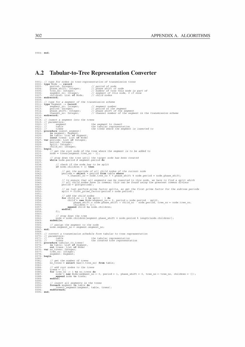
302 APPENDIX A. ALGORITHMS
0064: end;
A.2 Tabular-to-Tree Representation Converter
0001: // type for nodes in tree-representation of transmission trees0002: type Node := record0003: period: Integer; // period of node0004: phase_shift: Integer; // phase shift of node0005: tree_no: Integer; // number of tree this node is part of0006: segment_no: Integer; // segment of this node, 0 if none0007: children: List of Node; // child nodes0008: endrecord;0009:0010: // type for a segment of the transmission scheme0011: type Segment := record0012: segment_no: Integer; // segment number0013: period: Integer; // period of the segment0014: phase_shift: Integer; // phase shift of the segment0015: channel_no: Integer; // channel number of the segment in the transmission scheme0016: endrecord;0017:0018: // insert a segment into the trees0019: // parameters:0020: // segment the segment to insert0021: // table the tabular representation0022: // trees the trees where the segment is inserted to0023: procedure insert_segment(0024: in segment: Segment,0025: in table: List of Segment,0026: inout trees: List of Node)0027: var periods: List of Integer;0028: period: Integer;0029: split: Integer;0030: child_no: Integer;0031: begin0032: // get the root node of the tree where the segment is to be added to0033: node ← trees[segment.tree_no - 1];0034:0035: // step down the tree until the target node has been created0036: while node.period �= segment.period do0037:0038: // check if the node has to be split0039: if node.children = [] then0040:0041: // get the periods of all child nodes of the current node0042: periods ← select �.period from table where0043: �.channel_no ← node.tree_no ∧ �.phase_shift % node.period = node.phase_shift;0044:0045: // to ensure that all segments can be inserted to this node, we have to find a split which0046: // all child nodes have in common; this can be found using the greatest common divisor0047: period ← gcd(periods);0048:0049: // we just perform prime factor splits, so get the first prime factor for the subtree periods0050: split ← first_prime_factor(period ÷ node.period);0051:0052: // add the child nodes0053: for child_no := 0 to split - 1 do0054: child ← new Node(segment_no ← 0, period ← node.period · split,0055: phase_shift ← node.phase_shift + child_no · node.period, tree_no ← node.tree_no,0056: children ← []);0057: append child to node.children;0058: endfor;0059: fi;0060:0061: // step down the tree0062: node ← node.children[segment.phase_shift ÷ node.period % length(node.children)];0063: endwhile;0064:0065: // assign the segment to the node0066: node.segment_no ← segment.segment_no;0067: end;0068:0069: // convert a transmission schedule form tabular to tree representation0070: // parameters:0071: // table the tabular representation0072: // trees the created tree representation0073: procedure tabular_to_trees(0074: in table: List of Segment,0075: out trees: List of Node)0076: var no_trees: Integer;0077: tree_no: Integer;0078: segment: Segment;0079: begin0080:0081: // get the number of trees0082: no_trees ← select max(�.tree_no) from table;0083:0084: // add root nodes to the trees0085: trees ← [];0086: for tree_no := 1 to no_trees do0087: node ← new Node(segment_no ← 0, period ← 1, phase_shift ← 0, tree_no ← tree_no, children ← []);0088: append node to trees;0089: endfor;0090:0091: // insert all segments in the trees0092: foreach segment in table do0093: insert_segment(segment, table, trees);0094: endforeach;0095: end;

A.3. GENERALIZED GREEDY SCHEDULER 303
A.3 Generalized Greedy Scheduler
0001: // type for nodes in tree-representation of transmission trees0002: type Node := record0003: period: Integer; // period of node0004: phase_shift: Integer; // phase shift of node0005: tree_no: Integer; // number of tree this node is part of0006: segment_no: Integer; // segment of this node, 0 if none0007: children: List of Node; // child nodes0008: endrecord;0009:0010: // type for a segment of the transmission scheme0011: type Segment := record0012: segment_no: Integer; // segment number0013: required_period: Integer; // required transmission period of the segment0014: endrecord;0015:0016: // find the best split; this function remembers that there is a prime split restriction and decreases the0017: // split to apply accordingly0018: // parameters:0019: // required_period the required period of the segment0020: // node_period the period of the found node0021: // split_restriction prime factor split restriction to apply when performing splits0022: // best_split the calculated split to apply0023: procedure find_best_split(0024: in required_period: Integer,0025: in node_period: Integer,0026: in split_restriction: Integer,0027: out best_split: Integer)0028: var restriction_violated: Boolean;0029: current_node_period: Integer;0030: remaining_split: Integer;0031: begin0032:0033: // try as long until we found a split which does not violate the split restriction0034: restriction_violated ← true;0035: while restriction_violated do0036:0037: // check how much splitting is required0038: current_node_period ← node_period;0039: remaining_split ← required_period ÷ node_period;0040:0041: // perform one split after another as long as the split restriction is not violated0042: restriction_violated ← false;0043: while remaining_split > 1 ∧ ¬restriction_violated do0044:0045: // get the next prime split to perform0046: next_split ← smallest_prime_factor(remaining_split);0047:0048: // check if this split would violate the prime factor split restriction0049: restriction_violated ← (next_split ≥ split_restriction · current_node_period + 1);0050:0051: // calculate the remaining splits0052: remaining_split ← remaining_split ÷ next_split;0053: current_node_period ← current_node_period · next_split;0054: endwhile;0055:0056: // if this split failed, decrease required_period and try again0057: if restriction_violated then0058: required_period ← required_period - 1;0059: endif;0060: endwhile;0061: best_split ← required_period ÷ node_period;0062: end;0063:0064: // find the best node where a segment should be inserted0065: // parameters:0066: // segment the segment to insert0067: // available_nodes available nodes where the segment can be inserted0068: // weight weight value to use for selecting the node when several nodes qualify0069: // split_restriction prime factor split restriction to apply when performing splits0070: // best_node the best found node if any0071: // best_split the split to apply to this node0072: procedure find_best_node(0073: in segment: Segment,0074: in available_nodes: List of Node,0075: in weight: Real,0076: in split_restriction: Integer,0077: out best_node: Node,0078: out best_split: Integer)0079: var node: Node;0080: split: Integer;0081: quality1, quality2, quality, best_quality: Real;0082: begin0083:0084: // examine all available nodes0085: best_node ← ε;0086: best_split ← 0;0087: foreach node in available_nodes do0088:0089: // check if the node has a sufficiently low period0090: if node.period ≤ segment.required_period then0091:0092: // get the split we have to apply to this node0093: find_best_split(segment.required_period, node.period, split_restriction, split);0094:0095: // calculate the quality of this node0096: quality1 ← 1 - (segment.required_period - node.period · split) segment.required_period;0097: quality2 ← node.period segment.required_period;0098: quality ← weight · quality1 + (1 - weight) · quality2;0099:0100: // if this node is better than a previously found one, save it0101: if best_node = ε ∨ quality > best_quality then0102: best_node ← node;0103: best_quality ← quality;0104: best_split ← split;0105: endif;0106: endif;0107: endforeach;0108: end;0109:0110: // try to insert a segment into the transmission trees0111: // parameters:0112: // segment the segment to insert0113: // available_nodes available nodes where the segment can be inserted0114: // weight weight value to use for selecting the node when several nodes qualify
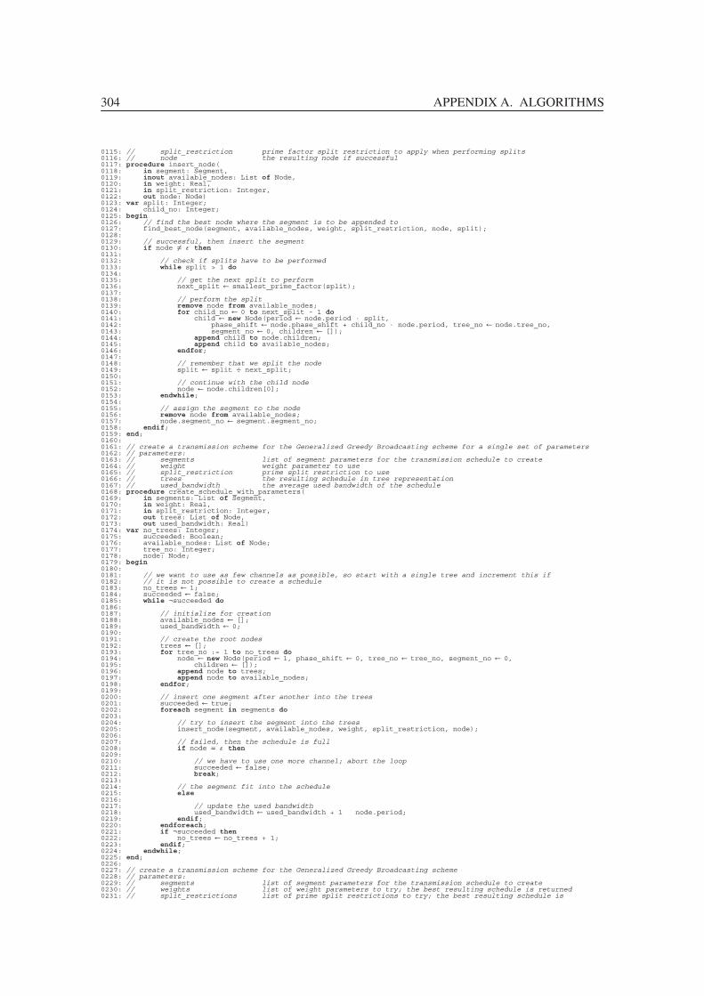
304 APPENDIX A. ALGORITHMS
0115: // split_restriction prime factor split restriction to apply when performing splits0116: // node the resulting node if successful0117: procedure insert_node(0118: in segment: Segment,0119: inout available_nodes: List of Node,0120: in weight: Real,0121: in split_restriction: Integer,0122: out node: Node)0123: var split: Integer;0124: child_no: Integer;0125: begin0126: // find the best node where the segment is to be appended to0127: find_best_node(segment, available_nodes, weight, split_restriction, node, split);0128:0129: // successful, then insert the segment0130: if node �= ε then0131:0132: // check if splits have to be performed0133: while split > 1 do0134:0135: // get the next split to perform0136: next_split ← smallest_prime_factor(split);0137:0138: // perform the split0139: remove node from available_nodes;0140: for child_no ← 0 to next_split - 1 do0141: child ← new Node(period ← node.period · split,0142: phase_shift ← node.phase_shift + child_no · node.period, tree_no ← node.tree_no,0143: segment_no ← 0, children ← []);0144: append child to node.children;0145: append child to available_nodes;0146: endfor;0147:0148: // remember that we split the node0149: split ← split ÷ next_split;0150:0151: // continue with the child node0152: node ← node.children[0];0153: endwhile;0154:0155: // assign the segment to the node0156: remove node from available_nodes;0157: node.segment_no ← segment.segment_no;0158: endif;0159: end;0160:0161: // create a transmission scheme for the Generalized Greedy Broadcasting scheme for a single set of parameters0162: // parameters:0163: // segments list of segment parameters for the transmission schedule to create0164: // weight weight parameter to use0165: // split_restriction prime split restriction to use0166: // trees the resulting schedule in tree representation0167: // used_bandwidth the average used bandwidth of the schedule0168: procedure create_schedule_with_parameters(0169: in segments: List of Segment,0170: in weight: Real,0171: in split_restriction: Integer,0172: out trees: List of Node,0173: out used_bandwidth: Real)0174: var no_trees: Integer;0175: succeeded: Boolean;0176: available_nodes: List of Node;0177: tree_no: Integer;0178: node: Node;0179: begin0180:0181: // we want to use as few channels as possible, so start with a single tree and increment this if0182: // it is not possible to create a schedule0183: no_trees ← 1;0184: succeeded ← false;0185: while ¬succeeded do0186:0187: // initialize for creation0188: available_nodes ← [];0189: used_bandwidth ← 0;0190:0191: // create the root nodes0192: trees ← [];0193: for tree_no := 1 to no_trees do0194: node ← new Node(period ← 1, phase_shift ← 0, tree_no ← tree_no, segment_no ← 0,0195: children ← []);0196: append node to trees;0197: append node to available_nodes;0198: endfor;0199:0200: // insert one segment after another into the trees0201: succeeded ← true;0202: foreach segment in segments do0203:0204: // try to insert the segment into the trees0205: insert_node(segment, available_nodes, weight, split_restriction, node);0206:0207: // failed, then the schedule is full0208: if node = ε then0209:0210: // we have to use one more channel; abort the loop0211: succeeded ← false;0212: break;0213:0214: // the segment fit into the schedule0215: else0216:0217: // update the used bandwidth0218: used_bandwidth ← used_bandwidth + 1 node.period;0219: endif;0220: endforeach;0221: if ¬succeeded then0222: no_trees ← no_trees + 1;0223: endif;0224: endwhile;0225: end;0226:0227: // create a transmission scheme for the Generalized Greedy Broadcasting scheme0228: // parameters:0229: // segments list of segment parameters for the transmission schedule to create0230: // weights list of weight parameters to try; the best resulting schedule is returned0231: // split_restrictions list of prime split restrictions to try; the best resulting schedule is

A.4. ENHANCED STARTUP 305
0232: // returned0233: // trees the resulting schedule in tree representation0234: // used_bandwidth the average used bandwidth of the schedule0235: procedure create_schedule(0236: in segments: List of Segment,0237: in weights: List of Real,0238: in split_restrictions: List of Integer,0239: out trees: List of Node,0240: out used_bandwidth: Real)0241: var weight: Real;0242: split_restriction: Integer;0243: current_trees: List of Node;0244: current_used_bandwidth: Real;0245: begin0246:0247: // sort the segments by their required period0248: sort segments ascending by required_period;0249:0250: // try all weights and prime split restrictions and return the schedule with the least average bandwidth0251: used_bandwidth ← ∞;0252: foreach weight in weights do0253: foreach split_restriction in split_restrictions do0254:0255: // create a schedule for these parameters0256: create_schedule_with_parameters(segments, weight, split_restriction,0257: current_trees, current_used_bandwidth);0258:0259: // if this schedule is better than previous ones, save it0260: if current_used_bandwidth < used_bandwidth then0261: trees ← current_trees;0262: used_bandwidth ← current_used_bandwidth;0263: endif;0264: endforeach;0265: endforeach;0266: end;
A.4 Enhanced Startup
0001: // type for nodes in tree-representation of transmission trees0002: type Node := record0003: period: Integer; // period of node0004: phase_shift: Integer; // phase shift of node0005: tree_no: Integer; // number of tree this node is part of0006: segment_no: Integer; // segment of this node, 0 if none0007: children: List of Node; // child nodes0008: endrecord;0009:0010: // type for extracted information from transmission trees0011: type Info := record0012: period: Integer; // period of a found node0013: no_children: Integer; // number of child nodes of the node0014: endrecord;0015:0016: // type for a segment of the transmission scheme0017: type Segment := record0018: segment_no: Integer; // segment number0019: required_period: Integer; // required transmission period of the segment0020: endrecord;0021:0022: // type for found positions in transmission trees where a segment can be inserted0023: type Position := record0024: tree_no: Integer; // tree number of the position0025: period: Integer; // period of the position0026: phase_shift: Integer; // phase shift of the position0027: splits: List of Integer; // splits which have to be performed0028: endrecord;0029:0030: // extract the structure of transmission trees0031: // parameters:0032: // node the node to examine0033: // infos list where to append the extracted information0034: procedure extract_structure_of_tree(0035: in node: Node,0036: inout infos: List of Info)0037: var child_node: Node;0038: begin0039:0040: // add the node itself0041: append new Info(period ← node.period, no_children ← length(node.children)) to infos;0042:0043: // add all child nodes of the node recursively0044: foreach child_node in node.children do0045: extract_structure_of_tree(child_node, infos);0046: endforeach;0047: end;0048:0049: // find the best position where a segment can be reinserted into the transmission trees when rebuilding the0050: // trees from the extracted information0051: // parameters:0052: // required_period required (i. e. maximum) period of the segment to insert0053: // min_period minimum period to use; needed to prevent that too many nodes with low period0054: // are consumed and insertion fails in the second round0055: // nodes list of node to examine for insertion or appending subtrees0056: // infos list of remaining information from tree structure extraction0057: // position the currently best position, is updated when a better one is found0058: procedure find_best_position(0059: in required_period: Integer,0060: in min_period: Integer,0061: in nodes: List of Node,0062: in infos: List of Info,0063: inout position: Position)0064: var node: Node;0065: begin0066:0067: // check all available nodes0068: foreach node in nodes do0069:0070: // check if the node has a sufficiently low period and is not yet used

306 APPENDIX A. ALGORITHMS
0071: if node.period ≤ required_period ∧ node.segment_no = 0 then0072:0073: // check if no child nodes have been added yet, i. e. if we can add a subtree0074: if node.children = [] then0075:0076: // search the best position by trying different subtree elements0077: find_best_position_with_reconstruction(required_period, min_period, node.tree_no,0078: node.period, node.phase_shift, infos, [], position);0079:0080: // otherwise child nodes have already been added, so look in them0081: else0082:0083: // look for good positions in the child nodes0084: find_best_position(required_period, min_period, node.children, infos, position);0085: endif;0086: endif;0087: endforeach;0088: end;0089:0090: // find the best position where a segment can be reinserted into the transmission trees when rebuilding the0091: // trees from the extracted information0092: // parameters:0093: // required_period required (i. e. maximum) period of the segment to insert0094: // min_period minimum period to use; needed to prevent that too many nodes with low period0095: // are consumed and insertion fails in the second round0096: // tree_no the tree number of the current node where information pieces can be added0097: // period the period of the current node where information pieces can be added0098: // phase_shift the phase shift of the current node where information pieces can be added0099: // infos list of remaining information from tree structure extraction0100: // splits list of splits which have already been performed to create this node0101: // position the currently best position, is updated when a better one is found0102: procedure find_best_position_with_reconstruction(0103: in required_period: Integer,0104: in min_period: Integer,0105: in tree_no: Integer,0106: in period: Integer,0107: in phase_shift: Integer,0108: in infos: List of Info,0109: in splits: List of Integer,0110: inout position: Position)0111: var info: Info;0112: child_no: Integer;0113: begin0114:0115: // examine all information pieces if one matches the period of the node0116: foreach info in infos do0117: if info.period = period then0118:0119: // if we have found a leaf node information piece and the period is high enough, we can try to0120: // add the segment here0121: if info.no_children = 0 ∧ period ≥ min_period then0122:0123: // check if the gained position is better than the previously found one0124: if position = ε ∨0125: (position.period + position.phase_shift ≥ required_period ∧0126: period + phase_shift < required_period) ∨0127: (period + phase_shift > position.period + position.phase_shift ∧0128: position.period + position.phase_shift ≥ required_period) ∨0129: (position.period + position.phase_shift < period + phase_shift ∧0130: period + phase_shift < required_period) then0131:0132: // update the currently best position with the found one0133: position ← new Position(tree_no ← tree_no, period ← period, phase_shift ← phase_shift,0134: splits ← splits);0135: endif;0136:0137: // otherwise the information piece describes a split0138: else0139:0140: // check if this split creates nodes with low enough period0141: if period · info.no_children ≤ required_period then0142:0143: // examine all resulting child nodes0144: for child_no ← 0 to info.no_children - 1 do0145: find_best_position_with_reconstruction(required_period, min_period, tree_no,0146: period · info.no_children, phase_shift + child_no · period, infos,0147: [splits, info.no_children], position);0148: endfor;0149: endif;0150: endif;0151: endif;0152: endforeach;0153: end;0154:0155: // reconstruct a node in the tree at a specified position and attach a segment to it0156: // parameters:0157: // segment_no the segment to attach to the resulting node0158: // phase_shift the phase shift of the node0159: // splits splits to perform to find the searched node0160: // node the (root) node where to reconstruct the node0161: // infos list of information pieces, used pieces are removed0162: procedure reconstruct_node_in_tree(0163: in segment_no: Segment,0164: in phase_shift: Integer,0165: in splits: List of Integer,0166: in node: Node,0167: inout infos: List of Info)0168: var info: Info;0169: child_no: Integer;0170: begin0171:0172: // skip the parts which already have been reconstructed0173: while node.children �= [] do0174: node ← node.children[phase_shift ÷ node.period % length(node.children)];0175: endwhile;0176:0177: // now perform the given splits0178: foreach split in splits do0179:0180: // remove the information piece which describes the current split from the list of available pieces0181: remove once from infos where infos[�].period = period ∧ infos[�].no_children = split;0182:0183: // create child nodes for the node to split0184: for child_no ← 0 to split - 1 do0185: child ← new Node(period ← node.period · split,0186: phase_shift ← node.phase_shift + child_no · node.period, tree_no ← node.tree_no,0187: segment_no ← 0, children ← []);

A.4. ENHANCED STARTUP 307
0188: append child to node.children;0189: endfor;0190:0191: // continue with the right child node0192: node ← node.children[phase_shift ÷ node.period % split];0193: endforeach;0194:0195: // remove the information piece which describes the current leaf node0196: remove once from infos where infos[�].period = period ∧ infos[�].no_children = 0;0197:0198: // attach the segment to the node0199: node.segment_no ← segment_no;0200: end;0201:0202: // get the minimum period when inserting a segment; this is necessary to prevent that all nodes with low0203: // periods are used up in the first round, producing a failure in the second round0204: // parameters:0205: // segments list of segments which still have to be inserted0206: // infos list of remaining information pieces from key structure extraction0207: // index index of the segment to insert in the segments list0208: // min_period the resulting minimum period to apply0209: procedure get_min_period(0210: in segments: List of Segment,0211: in infos: List of infos,0212: in index: Integer,0213: out min_period: Integer)0214: begin0215:0216: // examine the segments and infos in reverse order0217: while index > 0 ∧ segments[index - 1].required_period ≥ infos[index].period do0218: index ← index - 1;0219: endwhile;0220:0221: // the period of the information piece which cannot be inserted when the first information piece is0222: // removed describes the lower bound for the period0223: min_period ← infos[index].period;0224: end;0225:0226: // startup enhancement main function; rebuilds transmission trees in such a way that several segment0227: // transmissions can be omitted0228: // parameters:0229: // segments list of segments of this transmission schedule0230: // trees transmission schedule to optimize, will be replaced with the result0231: procedure enhance_startup(0232: in segments: List of Segment,0233: inout trees: List of Node)0234: var infos: List of Info;0235: segment: Segment;0236: no_trees: Integer;0237: tree_no: Integer;0238: position: Position;0239: int min_period: Integer;0240: int index: Integer;0241: begin0242:0243: // extract the information structure of the transmission schedule0244: infos ← [];0245: no_trees ← length(trees);0246: foreach tree in trees do0247: extract_structure_of_tree(tree, infos);0248: endforeach;0249:0250: // rebuild the root trees0251: trees ← [];0252: for tree_no ← 0 to no_trees - 1 do0253: append new Node(period ← 1, phase_shift ← 0, tree_no ← tree_no, segment_no ← 0, children ← []) to0254: trees;0255: endfor;0256:0257: // sort the segments and information pieces so they can simply be traversed0258: sort segments ascending by required_period;0259: sort infos ascending by no_children and ascending by period;0260:0261: // first round: insert only segments if they can be omitted at the first transmission0262: index ← 0;0263: while index < length(segments) do0264:0265: // get the segment to insert and its minimum period0266: segment ← segments[index];0267: get_min_period(segments, infos, index, min_period);0268:0269: // find the best position where to insert it into the transmission trees0270: position ← ε;0271: find_best_position(segment.required_period, min_period, trees, infos, position);0272:0273: // check if this position allows to omit the segment transmission once0274: if position.period + position.phase_shift < segment.required_period then0275:0276: // then reconstruct the corresponding nodes and insert the segment into the trees0277: reconstruct_node_in_tree(segment.segment_no, position.phase_shift, position.splits,0278: trees[position.tree_no], infos);0279:0280: // remove the segment from the list of segments to insert0281: remove segment from segments;0282:0283: // otherwise advance to the next segment0284: else0285: index ← index + 1;0286: endif;0287: endwhile;0288:0289: // round two: insert all remaining segments0290: while segments �= [] do0291:0292: // get the segment to insert0293: segment ← segments[0];0294:0295: // find the best position where to insert it into the transmission trees0296: position ← ε;0297: find_best_position(segment.required_period, 1, trees, infos, position);0298:0299: // reconstruct the corresponding nodes and insert the segment into the trees0300: reconstruct_node_in_tree(segment.segment_no, position.phase_shift, position.splits,0301: trees[position.tree_no], infos);0302:0303: // remove the segment from the list of segments to insert0304: remove segment from segments;

308 APPENDIX A. ALGORITHMS
0305: endwhile;0306: end;
A.5 Brute-Force Storage Requirement Calculation
0001: // type for a segment of the transmission scheme0002: type Segment := record0003: segment_no: Integer; // segment number0004: required_period: Integer; // required transmission period of the segment0005: period: Integer; // utilized period in the transmission scheme0006: phase_shift: Integer; // phase shift of the segment in the transmission scheme0007: channel_no: Integer; // channel number of the segment in the transmission scheme0008: endrecord;0009:0010: // type for specification of segment reception times0011: type Spec := record0012: segment_no: Integer; // segment number which is described0013: first: Integer; // the first recipient (in slot intervals after media startup) which0014: // received this segment0015: number: Integer; // the number of slot intervals this segment is received by receivers0016: period: Integer; // period of the segment0017: endrecord;0018:0019: // calculate storage requirements of a transmission scheme using the brute force approach0020: // parameters:0021: // segments the segments to examine0022: // t the playback time (in slot intervals) to calculate the storage requirements0023: // for0024: // storage_requirement the calculated storage requirement (in segments)0025: procedure calculate_storage_requirement(0026: in segments: List of Segment,0027: in t: Integer,0028: out storage_requirement: Integer)0029: var specs: List of Spec;0030: spec: Spec;0031: count: Integer;0032: s: Integer;0033: begin0034:0035: // calculate which segments are received under which circumstances (i. e. which join time); therefore0036: // examine all segments0037: specs ← [];0038: foreach segment in segments do0039:0040: // check if the segment has not yet been played0041: if t ≤ segment.needed_period - 1 then0042:0043: // calculate the join times of the receiver which received the segment first and the number0044: // of slot intervals of receivers which received the segment, too0045: first ← (segment.phase_shift - t) % segment.period;0046: number ← min(t + 1, segment.period, segment.period + t - segment.needed_period + 1);0047:0048: // if the segment is received (and will not be received again) by any receiver, save this0049: if number > 0 then0050: append new Spec(segment_no ← segment.segment_no, first ← first, number ← number,0051: period ← segment.period) to specs;0052: endif;0053: endif;0054: endforeach;0055:0056: // calculate the period of all specs we found0057: count ← 1;0058: foreach spec in specs do0059: count ← lcm(count, spec.period);0060: endforeach;0061:0062: // examine the storage requirements for all possible receivers0063: storage_requirement ← 0;0064: for s ← 0 to count - 1 do0065:0066: // calculate the storage requirements of a receiver which joined s slot intervals after media0067: // startup0068: new_storage_requirement ← 0;0069: foreach spec in specs do0070: if spec.number ≥ spec.period ∨ (s - spec.first) % spec.period < spec.number then0071: new_storage_requirement ← new_storage_requirement + 1;0072: endif;0073: endforeach;0074:0075: // if this result is higher than anything before, save it0076: if new_storage_requirement > storage_requirement then0077: storage_requirement ← new_storage_requirement;0078: endif;0079: endfor;0080: end;
A.6 Exact Storage Requirement Calculation
0001: // type for a segment of the transmission scheme0002: type Segment := record0003: segment_no: Integer; // segment number0004: required_period: Integer; // required transmission period of the segment0005: period: Integer; // utilized period in the transmission scheme0006: phase_shift: Integer; // phase shift of the segment in the transmission scheme0007: channel_no: Integer; // channel number of the segment in the transmission scheme0008: endrecord;0009:0010: // type for specification of segment reception times0011: type Spec := record
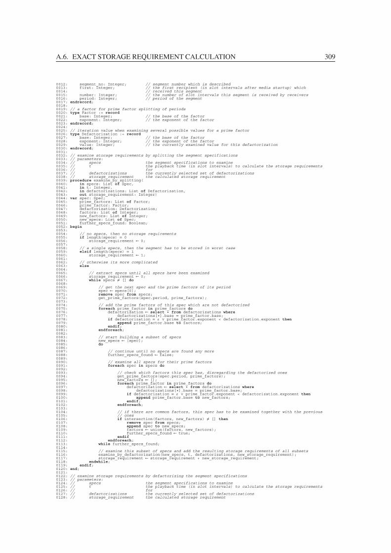
A.6. EXACT STORAGE REQUIREMENT CALCULATION 309
0012: segment_no: Integer; // segment number which is described0013: first: Integer; // the first recipient (in slot intervals after media startup) which0014: // received this segment0015: number: Integer; // the number of slot intervals this segment is received by receivers0016: period: Integer; // period of the segment0017: endrecord;0018:0019: // a factor for prime factor splitting of periods0020: type Factor := record0021: base: Integer; // the base of the factor0022: exponent: Integer; // the exponent of the factor0023: endrecord;0024:0025: // iteration value when examining several possible values for a prime factor0026: type Defactorization := record0027: base: Integer; // the base of the factor0028: exponent: Integer; // the exponent of the factor0029: value: Integer; // the currently examined value for this defactorization0030: endrecord;0031:0032: // examine storage requirements by splitting the segment specifications0033: // parameters:0034: // specs the segment specifications to examine0035: // t the playback time (in slot intervals) to calculate the storage requirements0036: // for0037: // defactorizations the currently selected set of defactorizations0038: // storage_requirement the calculated storage requirement0039: procedure examine_by_splitting(0040: in specs: List of Spec,0041: in t: Integer,0042: in defactorizations: List of Defactorization,0043: out storage_requirement: Integer)0044: var spec: Spec;0045: prime_factors: List of Factor;0046: prime_factor: Factor;0047: defactorization: Defactorization;0048: factors: List of Integer;0049: new_factors: List of Integer;0050: new_specs: List of Spec;0051: further_specs_found: Boolean;0052: begin0053:0054: // no specs, then no storage requirements0055: if length(specs) = 00056: storage_requirement ← 0;0057:0058: // a single specs, then the segment has to be stored in worst case0059: elsif length(specs) = 10060: storage_requirement ← 1;0061:0062: // otherwise its more complicated0063: else0064:0065: // extract specs until all specs have been examined0066: storage_requirement ← 0;0067: while specs �= [] do0068:0069: // get the next spec and the prime factors of its period0070: spec ← specs[0];0071: remove spec from specs;0072: get_prime_factors(spec.period, prime_factors);0073:0074: // add the prime factors of this spec which are not defactorized0075: foreach prime_factor in prime_factors do0076: defactorization ← select � from defactorizations where0077: defactorizations[�].base = prime_factor.base;0078: if defactorization = ε ∨ prime_factor.exponent < defactorization.exponent then0079: append prime_factor.base to factors;0080: endif;0081: endforeach;0082:0083: // start building a subset of specs0084: new_specs ← [spec];0085: do0086:0087: // continue until no specs are found any more0088: further_specs_found ← false;0089:0090: // examine all specs for their prime factors0091: foreach spec in specs do0092:0093: // check which factors this spec has, disregarding the defactorized ones0094: get_prime_factors(spec.period, prime_factors);0095: new_factors ← [];0096: foreach prime_factor in prime_factors do0097: defactorization ← select � from defactorizations where0098: defactorizations[�].base = prime_factor.base;0099: if defactorization = ε ∨ prime_factor.exponent < defactorization.exponent then0100: append prime_factor.base to new_factors;0101: endif;0102: endforeach;0103:0104: // if there are common factors, this spec has to be examined together with the previous0105: // ones0106: if intersection(factors, new_factors) �= [] then0107: remove spec from specs;0108: append spec to new_specs;0109: factors ← union(factors, new_factors);0110: further_specs_found ← true;0111: endif0112: endforeach;0113: while further_specs_found;0114:0115: // examine this subset of specs and add the resulting storage requirements of all subsets0116: examine_by_defactorization(new_specs, t, defactorizations, new_storage_requirement);0117: storage_requirement ← storage_requirement + new_storage_requirement;0118: endwhile;0119: endif;0120: end;0121:0122: // examine storage requirements by defactorizing the segment specifications0123: // parameters:0124: // specs the segment specifications to examine0125: // t the playback time (in slot intervals) to calculate the storage requirements0126: // for0127: // defactorizations the currently selected set of defactorizations0128: // storage_requirement the calculated storage requirement
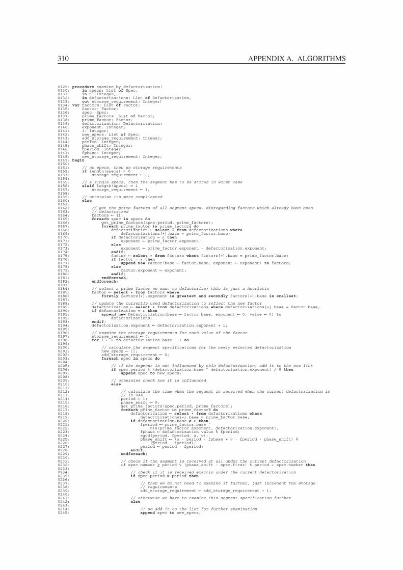
310 APPENDIX A. ALGORITHMS
0129: procedure examine_by_defactorization(0130: in specs: List of Spec,0131: in t: Integer,0132: in defactorizations: List of Defactorization,0133: out storage_requirement: Integer)0134: var factors: List of Factor;0135: factor: Factor;0136: spec: Spec;0137: prime_factors: List of Factor;0138: prime_factor: Factor;0139: defactorization: Defactorization;0140: exponent: Integer;0141: i: Integer;0142: new_specs: List of Spec;0143: add_storage_requirement: Integer;0144: period: Integer;0145: phase_shift: Integer;0146: fperiod: Integer;0147: fphase: Integer;0148: new_storage_requirement: Integer;0149: begin0150:0151: // no specs, then no storage requirements0152: if length(specs) = 00153: storage_requirement ← 0;0154:0155: // a single specs, then the segment has to be stored in worst case0156: elsif length(specs) = 10157: storage_requirement ← 1;0158:0159: // otherwise its more complicated0160: else0161:0162: // get the prime factors of all segment specs, disregarding factors which already have been0163: // defactorized0164: factors ← [];0165: foreach spec in specs do0166: get_prime_factors(spec.period, prime_factors);0167: foreach prime_factor in prime_factors do0168: defactorization ← select � from defactorizations where0169: defactorizations[�].base = prime_factor.base;0170: if defactorization = ε then0171: exponent ← prime_factor.exponent;0172: else0173: exponent ← prime_factor.exponent - defactorization.exponent;0174: endif;0175: factor ← select � from factors where factors[�].base = prime_factor.base;0176: if factor = ε then0177: append new Factor(base ← factor.base, exponent ← exponent) to factors;0178: else0179: factor.exponent ← exponent;0180: endif;0181: endforeach;0182: endforeach;0183:0184: // select a prime factor we want to defactorize; this is just a heuristic0185: factor ← select � from factors where0186: firstly factors[�].exponent is greatest and secondly factors[�].base is smallest;0187:0188: // update the currently used defactorization to reflect the new factor0189: defactorization ← select � from defactorizations where defactorizations[�].base = factor.base;0190: if defactorization = ε then0191: append new Defactorization(base ← factor.base, exponent ← 0, value ← 0) to0192: defactorizations;0193: endif;0194: defactorization.exponent ← defactorization.exponent + 1;0195:0196: // examine the storage requirements for each value of the factor0197: storage_requirement ← 0;0198: for i ← 0 to defactorization.base - 1 do0199:0200: // calculate the segment specifications for the newly selected defactorization0201: new_specs ← [];0202: add_storage_requirement ← 0;0203: foreach spec in specs do0204:0205: // if the segment is not influenced by this defactorization, add it to the new list0206: if spec.period % (defactorization.base ˆ defactorization.exponent) �= 0 then0207: append spec to new_specs;0208:0209: // otherwise check how it is influenced0210: else0211:0212: // calculate the time when the segment is received when the current defactorization is0213: // in use0214: period ← 1;0215: phase_shift ← 0;0216: get_prime_factors(spec.period, prime_factors);0217: foreach prime_factor in prime_factors do0218: defactorization ← select � from defactorizations where0219: defactorizations[�].base = prime_factor.base;0220: if defactorization.base �= ε then0221: fperiod ← prime_factor.base ˆ0222: min(prime_factor.exponent, defactorization.exponent);0223: fphase ← defactorization.value % fperiod;0224: egcd(period, fperiod, u, v);0225: phase_shift ← (u · period · fphase + v · fperiod · phase_shift) %0226: (period · fperiod);0227: period ← period · fperiod;0228: endif;0229: endforeach;0230:0231: // check if the segment is received at all under the current defactorization0232: if spec.number ≥ period ∨ (phase_shift - spec.first) % period < spec.number then0233:0234: // check if it is received exactly under the current defactorization0235: if spec.period = period then0236:0237: // then we do not need to examine it further, just increment the storage0238: // requirements0239: add_storage_requirement ← add_storage_requirement + 1;0240:0241: // otherwise we have to examine this segment specification further0242: else0243:0244: // so add it to the list for further examination0245: append spec to new_specs;

A.7. FAST STORAGE REQUIREMENT ESTIMATION 311
0246: endif;0247: endif;0248: endif;0249: endforeach;0250:0251: // examine the reduced set of segment specifications0252: examine_by_splitting(new_specs, t, defactorizations, new_storage_requirement);0253:0254: // if the resulting storage requirements are higher than the previous ones, remember the new0255: // result0256: if new_storage_requirement + add_storage_requirement > storage_requirement then0257: storage_requirement ← new_storage_requirement + add_storage_requirement;0258: endif;0259:0260: // update the defactorization value0261: defactorization.value ← defactorization.value +0262: defactorization.base ˆ (defactorization.exponent - 1);0263: endfor;0264: endif;0265: end;0266:0267: // calculate exact storage requirements0268: // parameters:0269: // segments the segments to examine0270: // t the playback time (in slot intervals) to calculate the storage requirements0271: // for0272: // storage_requirement the calculated storage requirement0273: procedure calculate_storage_requirement(0274: in segments: List of Segment,0275: in t: Integer,0276: out storage_requirement: Integer)0277: var specs: List of Spec;0278: begin0279:0280: // calculate which segments are received under which circumstances (i. e. which join time); therefore0281: // examine all segments0282: specs ← [];0283: foreach segment in segments do0284:0285: // check if the segment has not yet been played0286: if t ≤ segment.needed_period - 1 then0287:0288: // calculate the join times of the receiver which received the segment first and the number0289: // of slot intervals of receivers which received the segment, too0290: first ← (segment.phase_shift - t) % segment.period;0291: number ← min(t + 1, segment.period, segment.period + t - segment.needed_period + 1);0292:0293: // if the segment is received (and will not be received again) by any receiver, save this0294: if number > 0 then0295: append new Spec(segment_no ← segment.segment_no, first ← first, number ← number,0296: period ← segment.period) to specs;0297: endif;0298: endif;0299: endforeach;0300:0301: // start calculation0302: examine_by_splitting(specs, t, [], storage_requirement);0303: end
A.7 Fast Storage Requirement Estimation
0001: // type for nodes in tree-representation of transmission trees0002: type Node := record0003: period: Integer; // period of node0004: phase_shift: Integer; // phase shift of node0005: tree_no: Integer; // number of tree this node is part of0006: segment_no: Integer; // segment of this node, 0 if none0007: children: List of Node; // child nodes0008: endrecord;0009:0010: // type for a segment of the transmission scheme0011: type Segment := record0012: segment_no: Integer; // segment number0013: required_period: Integer; // required transmission period of the segment0014: period: Integer; // utilized period in the transmission scheme0015: phase_shift: Integer; // phase shift of the segment in the transmission scheme0016: channel_no: Integer; // channel number of the segment in the transmission scheme0017: endrecord;0018:0019: // calculate the storage requirements for a single node0020: // t the playback time (in slot intervals) to calculate the storage requirements0021: // for0022: // number the number of transmissions of this node since joining the transmission0023: // node the node to examine0024: // storage_requirement the calculated storage requirement0025: procedure examine_node(0026: in t: Integer,0027: in number: Integer,0028: in node: Node,0029: out storage_requirement: Integer)0030: var child: Node;0031: i: Integer;0032: j: Integer;0033: low: List of Integer;0034: hi: List of Integer;0035: add_storage_requirement: Integer;0036: begin0037:0038: // check if the node has been transmitted at all0039: storage_requirement ← 0;0040: if number > 0 then0041:0042: // check if the node is a leaf node0043: if length(node.children) = 0 then0044:0045: // check if the node has a segment attached to it0046: if node.segment_no �= 0 then0047:
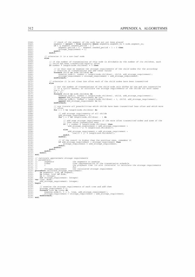
312 APPENDIX A. ALGORITHMS
0048: // check if the segment of the node has not yet been played0049: segment ← select � from segments where segments.segment_no = node.segment_no;0050: if t ≤ segment.needed_period - 1 ∧0051: segment.period + t - segment.needed_period + 1 > 0 then0052: storage_requirement ← 1;0053: endif;0054: endif;0055:0056: // otherwise it is a non-leaf node0057: else0058:0059: // if the number of transmissions of this node is dividable by the number of its children, each0060: // child has been transmitted equally often0061: if number % length(node.children) = 0 then0062:0063: // in this case we examine the storage requirements of the child nodes for the according0064: // fraction of transmissions and add these values0065: foreach child in node.children do0066: examine_node(t, number ÷ length(node.children), child, add_storage_requirement);0067: storage_requirement ← storage_requirement + add_storage_requirement;0068: endforeach;0069:0070: // otherwise it is not clear how often each of the child nodes have been transmitted0071: else0072:0073: // but the number of transmissions of the child node only differ by one and are consecutive0074: // in a cyclic manner; so calculate the storage requirements of the childs for both cases0075: low ← [];0076: hi ← [];0077: foreach child in node.children do0078: examine_node(t, number ÷ length(node.children), child, add_storage_requirement);0079: append add_storage_requirement to low;0080: examine_node(t, number ÷ length(node.children) + 1, child, add_storage_requirement);0081: append add_storage_requirement to hi;0082: endforeach;0083:0084: // now iterate all possibilities which childs have been transmitted less often and which more0085: // often0086: for i ← 0 to length(node.children) do0087:0088: // add storage requirements of all childs0089: add_storage_requirement ← 0;0090: for j ← 0 to length(node.children) - 1 do0091:0092: // add some storage requirements of the more often transmitted nodes and some of the0093: // less often transmitted ones0094: if j < number % length(node.children) then0095: add_storage_requirement ← add_storage_requirement +0096: hi[(i + j) % length(nod.children)];0097: else0098: add_storage_requirement ← add_storage_requirement +0099: low[(i + j) % length(nod.children)];0100: endif;0101: endfor;0102:0103: // if the result is higher than the previous ones, remember it0104: if add_storage_requirement > storage_requirement then0105: storage_requirement ← add_storage_requirement;0106: endif;0107: endfor;0108: endif;0109: endif;0110: endif;0111: end;0112:0113: // calculate approximate storage requirements0114: // parameters:0115: // segments the segments to examine0116: // trees tree representation of the transmission schedule0117: // t the playback time (in slot intervals) to calculate the storage requirements0118: // for0119: // storage_requirement the calculated storage requirement0120: procedure calculate_storage_requirement(0121: in segments: List of Segment,0122: in trees: List of Node,0123: in t: Integer,0124: out storage_requirement: Integer)0125: var tree: Node;0126: add_storage_requirement: Integer;0127: begin0128:0129: // examine the storage requirements of each tree and add them0130: storage_requirement ← 0;0131: foreach tree in trees do0132: examine_node(t, t + 1, tree, add_storage_requirement);0133: storage_requirement ← storage_requirement + add_storage_requirement;0134: endforeach;0135: end;

Appendix B
Nomenclature
IN this thesis, symbol names in equations have been used uniformly wherever possible. The
following table provides a reference of the used symbol, its meaning and unit. For scalar values,
the unit is displayed as 1, for functions, domain and codomain are separated by an arrow (→).
Symbol Description Unit
b bandwidth of media stream (only applicable for constant-bit-
rate media streams)
bytes
s
d total duration of media stream s
f (t) cumulative bandwidth function, f (t) is the position of the first
byte in the media stream which is played at time t after begin-
ning of playback
s→ bytes
f−1(p) inverse cumulative bandwidth function, f−1(p) is the time
stamp in the media stream when the position p is reached
bytes→ s
n number of segments of the media stream 1
s size of media stream bytes
B total sender bandwidth of the transmissionbytes
s
B− theoretical lower bound for Bbytes
s
B◦ average total sender bandwidth of the transmissionbytes
s
Bi bandwidth of channel #ibytes
s
C fraction for lowering channel bandwidth 1
F (t) playback function of the receiver system, based on the utilized
playback delay; F (t) is the position in the media stream which
is played at time t
s→ bytes
F−(t) playback function of the receiver system, based on the minimum
playback delay
s→ bytes

314 APPENDIX B. NOMENCLATURE
Symbol Description Unit
F+(t) playback function of the receiver system, based on the maxi-
mum playback delay
s→ bytes
F−1(p) inverse playback function, based on utilized playback delay bytes→ s
F−−1(p) inverse playback function, based on minimum playback delay bytes→ s
F+−1(p) inverse playback function, based on maximum playback delay bytes→ s
F (t) antiderivative of the playback function s
J protocol specific latency for leaving and joining a channel s
Ji joining latency of channel #i relative to beginning of reception s
L Prime split limit; if⌊
π+i
ΠN
⌋≥ L ·ΠN +1, a prime split of a node
is prohibited
1
N number of channels of the transmission 1
P size of preloaded amount of media stream bytes
M+(t) worst case storage requirement function, M+(t) gives the worst
case storage requirement of a playback at time t
s→ bytes
Pi total period of channel #i 1
P+i imposed limit on Pi 1
Qi,N quality value for scheduling segment #i at node N, used to find
the best node in the scheduling algorithm
1
QIi,N first of the quality values which are combined to Qi,N 1
QIIi,N second of the quality values which are combined to Qi,N 1
QIIIi,N
third of the quality values which are combined to Qi,N 1
R number of channels the receiver system can receive simultane-
ously
1
S broadcasting series of size-based transmission schemes 1→ 1
Tplaybackdelay(t) transmission function for additional playback delay s→ s
Tpartialpreloading(p) transmission function for partial preloading bytes→ bytes
Tbreakinsertion(t) transmission function for break insertion s→ s
W − minimum possible playback delay for the transmission s
W + maximum possible playback delay for the transmission s
W ◦ average playback delay for the transmission s
W II weight for weighting of QIIi,N
in Qi,N 1
W III weight for weighting of QIIIi,N
in Qi,N 1
β bandwidth of each segment transmission/bandwidth of each
channel, β = σδ
bytes
s
βi bandwidth of segment #i in the schedulebytes
s

315
Symbol Description Unit
δ slot interval = transmission duration of one segment s
δi duration of a segment #i s
κi channel number which is used for segment #i in the schedule;
symbol taken from the Greek word καναλι
1
πi utilized period of segment #i in the schedule; symbol taken from
the Greek word περιoδoς
1
π+i maximum period of segment #i which is needed in the schedule
for proper playback
1
σ size of segments bytes
σi size of segment #i bytes
τi playback time of segment #i s
φi phase shift of segment #i, 0 ≤ φi < πi; symbol taken from the
Greek word φαση
1
KN channel number which is used for node #i in the schedule 1
ΠN utilized period of node #N in the schedule 1
ΦN phase shift of node #N, 0 ≤Φi <Πi 1
η efficiency of a transmission schedule, 0 < η ≤ 1 1
e Euler’s number, the base of the natural logarithm (e ≈2.718281828)
1
γ Euler-Mascheroni constant (γ ≈ 0.577215665) 1
The following mathematical symbols, functions and operators have been used throughout this
thesis:
Operator Description
∞ infinity
�� truncation to next integer (towards −∞)
� rounding up to next integer (towards +∞)
◦ function composition, (f ◦ g)(x) = f (g(x))
∧ logical and
∨ logical or
div integer division, a div b =⌊ab
⌋gcd greatest common divisor
lcm least common multiple
mod integer modulo, a mod b = a−b · ⌊ab
⌋

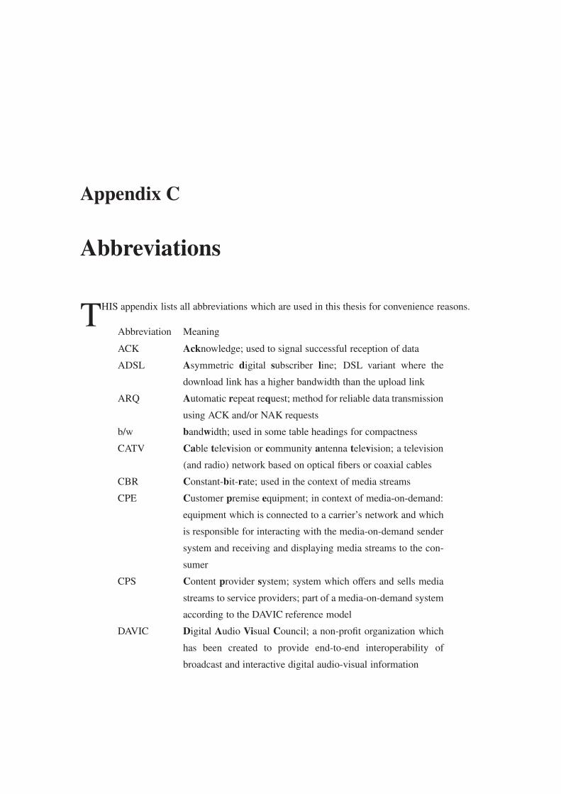
Appendix C
Abbreviations
THIS appendix lists all abbreviations which are used in this thesis for convenience reasons.
Abbreviation Meaning
ACK Acknowledge; used to signal successful reception of data
ADSL Asymmetric digital subscriber line; DSL variant where the
download link has a higher bandwidth than the upload link
ARQ Automatic repeat request; method for reliable data transmission
using ACK and/or NAK requests
b/w bandwidth; used in some table headings for compactness
CATV Cable television or community antenna television; a television
(and radio) network based on optical fibers or coaxial cables
CBR Constant-bit-rate; used in the context of media streams
CPE Customer premise equipment; in context of media-on-demand:
equipment which is connected to a carrier’s network and which
is responsible for interacting with the media-on-demand sender
system and receiving and displaying media streams to the con-
sumer
CPS Content provider system; system which offers and sells media
streams to service providers; part of a media-on-demand system
according to the DAVIC reference model
DAVIC Digital Audio Visual Council; a non-profit organization which
has been created to provide end-to-end interoperability of
broadcast and interactive digital audio-visual information
318 APPENDIX C. ABBREVIATIONS
Abbreviation Meaning
DSL Digital subscriber line; a common type of home Internet ac-
cess using telephone lines; compared to traditional home Inter-
net access via acoustic modems or ISDN, DSL provides a much
higher data rate (currently up to 15 Mbit/s)
DVD Digital versatile disk
EUR Currency of the European Currency Union
FCFS First come first served; scheduling strategy where the requests
are served one after another in the order of requests
FEC Forward error correction; increasing reliability of a transmis-
sion by adding redundancy to support recovery of lost data
ISDN Integrated services digital network; a type of digital, circuit
switched telephone network which is capable to transmit both
voice and digital data; sometimes used for home Internet access
(providing a data rate of up to 128 Kbit/s on copper telephone
lines)
MFQL Maximum factored queue length; strategy where the requests
are grouped in queued depending on the requested media stream
and served sorted by queue length times a queue specific factor,
starting with the longest product
MQL Maximum queue length; batching strategy where the requests
are grouped in queued depending on the requested media stream
and served sorted by queue length, starting with the longest
queue
NAK Negative acknowledge; used to signal data losses
RTCP Real-time transport control protocol; protocol for transmission
of auxiliary data (e. g. for stream synchronization and reception
quality feedback) for an RTP transmission
RTP Real-time transport protocol; protocol for transmission of data
streams with timed delivery
SCS Service consumer system; system which allows a consumer
to receive a media stream from a service provider system and
which is implemented in a customer premise equipment; part of
a media-on-demand system according to the DAVIC reference
model

319
Abbreviation Meaning
SDP Session description protocol; protocol for describing and an-
nouncing multimedia session parameters
SIP Session initiation protocol; protocol for initiating and control-
ling multimedia sessions
SPS Service provider system; system which keeps media streams
from a content provider system in its media database and which
accepts and processes schedules (either fixed ones or based on
requests) for delivery of media streams to service consumer
systems; part of a media-on-demand system according to the
DAVIC reference model
STB Set-top box; a device which receives data from a network (ca-
ble, satellite, radio broadcast) and prepares it for displaying on
a TV system
TV Television
US, USA United States (of America)
USD United States Dollar; see below for exchange rate which has
been used throughout this thesis
VBR Variable-bit-rate; used in the context of media streams
VCR Video cassette recorder
VDSL Very high data rate digital subscriber line; ADSL successor
which provides a download bit rate of up to 51.85 Mbit/s
For the cost analysis in chapter 6 in this thesis, results from various marketing studies have been
used. Where values must be compared or are included in calculations, they have been converted to
euro (EUR), the currency unit of the European currency union. The following exchange rate for
United States dollar (USD) has been taken on April 23, 2008 and has been used within this thesis:
1.00 EUR = 1.59 USD
The results of currency conversions have been rounded to a precision of three digits.


Appendix D
Typesetting Conventions
FOR improved clearness, the following typesetting rules have have been used throughout this
thesis:
• Definitions of terms which are used unambiguously in this thesis are printed in bold letters:
Media-on-demand is a technique for transmitting media streams from media-
on-demand sender systems to media-on-demand receiver systems in real-
time.
• To emphasize text, italics is used:
With media-on-demand, the viewers can select themselves what to see and the
time when to see it.
• Quotations are typed in italics and indented left and right:
Video on Demand (VOD) is a technology to view and order video content as and
when required in the home [. . . ].
• Program code is printed in a small fixed width font, prefixing each line with a line number
and using bold letters for keywords:
0001: // calculate the greatest common divisor of two integers0002: // parameters:0003: // f the first integer0004: // g the second integer0005: // result the greatest common divisor of f and g0006: procedure gcd(0007: in f: Integer,0008: in g: Integer,0009: out result: Integer)0010: var remainder: Integer;0011: begin0012:0013: // use euclidean algorithm for calculation0014: while g �= 0 do0015: remainder ← f % g;0016: f ← g;0017: g ← remainder;0018: endwhile;0019:0020: // return the result0021: result ← f;0022: end;

322 APPENDIX D. TYPESETTING CONVENTIONS
• Equations are written indented and are labeled at the right margin. Symbols in equations are
always set in italic type and follow additionally these conventions:
– Values related to segments are represented using lowercase Greek letters, suffixed by
an index which denotes the segment number where needed:
Segment #i has period πi.
– For values related to nodes of the tree representation of a transmission scheme, upper-
case Greek letters, suffixed by a node where needed:
Node #N has period ΠN .
– For values related to the media stream, lowercase Roman letters are used:
The total duration of the media stream is d.
– To represent values specific to a media stream transmission, uppercase Roman letters
are utilized:
The total sender bandwidth is B.
Regardless of these rules, η is used for the efficiency of transmission schemes due to com-
mon conventions.
• Numbers are shown in groups of three digits, using a period as decimal point:
π10 ≈ 93648.047477
Opposed to this rule, years are given in a single group:
In year 2000, (opposed to 2 000 segments) . . .
• Citations are shown in brackets, using the first three characters of the last name of the author
in case of a single author, the initials of the last names of all authors in case of two to four
authors or the initials of the last names of the first four authors suffixed by a plus sign if the
citation has more than four authors, always followed by the year of publication:
In [BNL02], the authors proposed . . .

Appendix E
Available Media-on-Demand Systems
SINCE 1990 when the first commercial video-on-demand service was offered in Hong Kong
[Wik08e, Oft03], many companies entered the video-on-demand market and developed their
own systems. But nearly all media-on-demand systems are still based on simple media-on-demand
transmission schemes. Table E.1 and E.2 show a list of currently available video-on-demand
solutions, the supported transmission scheme1 and web links to web locations where all data about
the systems has been retrieved.
Most of these systems are based on one of the following three transmission schemes:
• Point-to-Point Transmissions: Most of the media-on-demand systems use Point-to-Point
connections for streaming media. The video-on-demand architecture recommendation “De-
mand Adaptive and Locality Aware (DALA) streaming media server cluster architecture”
[GJS02] and the video-on-demand system architecture of the “Digital Audio Visual Coun-
cil” [Dav99] are based on Point-to-Point transmissions.
• Single Broadcast: Some of the systems support media broadcast (often including live broad-
cast) using multicasting, unfortunately only at predefined time and frequency.
• Complete Prefetching: Although none of the companies in the list sell Media-on-Demand
systems using Complete Prefetching, many of them have a (non-real-time) content distribu-
tion product which may be used for this purpose.
The only exception the author of this thesis has knowledge of which uses an enhanced media-
on-demand transmission scheme (the original Greedy Broadcasting scheme) is the TelliVision
system from Tellitec Communications bvba, a system which has been developed partially by the
author.
Many other companies are involved in media-on-demand techniques, too, e. g. by developing
specialized video streaming hardware. But as this thesis focuses to media-on-demand transmission
1The list of supported transmission schemes may be incomplete in some cases because of missing information in
product descriptions.

324APPENDIXE.AVAILABLEMEDIA-ON-DEMANDSYSTEMS
Co
mp
any
Sy
stem
Sch
eme
Ref
eren
ces
Ap
ple
Co
mp
ute
r,In
c.Q
uic
kti
me
Bro
adca
ster
,
Qu
ick
tim
eS
trea
min
g
Ser
ver
,D
arw
inS
trea
min
g
Ser
ver
SB
,P
tPhttp://www.apple.com/de/quicktime/broadcaster/
Cis
coS
yst
ems,
Inc.
Cis
coIP
TV
vid
eose
rver
PtP
,S
Bhttp://www.cisco.com/en/US/netsol/ns340/ns394/
ns158/ns88/networking_solutions_package.html
Co
mp
agn
ieF
inan
cièr
e
Alc
atel
Alc
atel
Op
enM
edia
Co
nte
nt
Man
ager
PtP
,S
Bhttp://www.alcatel.de/products/productsummary.
jhtml?repositoryID=/com/en/appxml/opgproduct/
alcatel5959openmediacontentmanagertcm228121551635.
jhtml
Co
ncu
rren
tC
om
pu
ter
Co
rp.
Med
iaH
awk
PtP
http://www.adelphia.com/pdf/Adelphia_LA_VOD.pdf
Env
ivio
,In
c.E
nv
ivio
4C
aste
r/IP
TV
PtP
,S
Bhttp://www.envivio.com/solutions/iptv.php
Hew
lett
-Pac
kar
d
Dev
elo
pm
entC
om
pan
y,
L.P.
HP
IPT
VP
tP,S
Bhttp://h71028.www7.hp.com/enterprise/cache/
312831-0-0-225-121.html
IBM
Co
rp.
IPT
VP
tPhttp://www-03.ibm.com/servers/eserver/xseries/
solutions/ind/iptv_overview.html
Info
Val
ue
Co
mp
uti
ng
,In
c.Q
uic
kV
ideo
PtP
,S
Bhttp://www.infovalue.com/products/product.htm
Kas
enn
aK
asen
na
Med
iaB
ase
vid
eo
serv
erso
ftw
are
PtP
,S
Bhttp://www.kasenna.com/solutions/products/
mediabase_xmp.php
Min
erva
Net
wo
rks,
Inc.
iTV
Man
ager
PtP
,S
Bhttp://www.minervanetworks.com/images/
itvManager2.pdf
PtP=
Po
int-
to-P
oin
t,S
B=
Sin
gle
Bro
adca
stin
g,G
B=
Gre
edy
Bro
adca
stin
g
Tab
leE
.1:
Avai
lable
med
ia-o
n-d
eman
dsy
stem
s(s
elec
tion
)

325
Co
mp
any
Sy
stem
Sch
eme
Ref
eren
ces
Net
scap
eC
om
mu
nic
atio
ns,
Co
rp./
Inso
ftN
etw
ork
Tel
evis
ion
,C
orp
.
INT
V!
PtP
http://wp.netscape.com/newsref/pr/newsrelease81.
html
Ora
cle
Co
rp.
Ora
cle
Med
iaS
erver
PtP
http://www.vccs.edu/its/projects/oracle/ovs-gl1.
htm
Rea
lNet
wo
rks,
Inc.
Hel
ixS
erver
PtP
,S
Bhttp://www.realnetworks.com/products/media_
delivery.html
Sea
Ch
ang
eS
eaC
han
ge
IPV
ideo
So
luti
on
s
PtP
,S
Bhttp://www.schange.com/Products/IP_Video/Main.asp
Sta
rlig
ht
Net
wo
rks
Sta
rWo
rks
PtP
http://www.highbeam.com/library/docfree.
asp?DOCID=1G1:18742882\&ctrlInfo=Round19
%3AMode19b%3ADocG%3AResult\&ao=
Sto
ny
Bro
ok
Un
iver
sity
Sto
ny
Bro
ok
Vid
eoS
erver
PtP
http://www.ecsl.cs.sunysb.edu/~andrew/
VideoServer/videoserver/index/book1.html
Su
nS
how
Me
Su
nM
icro
syst
ems
SB
http://www.sun.com/products-n-solutions/hardware/
docs/pdf/802-6020-13.pdf
New
tec
Cy
N.
V.
Tel
liV
isio
nP
tP,
GB
http://www.tellitec.be/tellivision/index.html
Th
ird
spac
eL
ivin
gL
td.
Th
ird
spac
eO
pen
Vid
eo
Ser
ver
PtP
http://ccur.com/corp_news_pressrelease.asp?
pressreleaseid=269
Un
iver
sity
of
Ber
kel
eyB
erkel
eyD
istr
ibu
ted
Vid
eo-o
n-D
eman
dS
yst
em
PtP
http://bmrc.berkeley.edu/frame/research/storage/
Tab
leE
.2:
Avai
lable
Med
ia-o
n-D
eman
dS
yst
ems
(PtP=
Poin
t-to
-Poin
t,S
B=
Sin
gle
Bro
adca
stin
g,
GB=
Gre
edy
Bro
adca
stin
g)

326 APPENDIX E. AVAILABLE MEDIA-ON-DEMAND SYSTEMS
techniques, a comparison of different hardware systems for media-on-demand is beyond the scope
of this thesis.
Bibliography
[ABEL94] A. Albanese, J. Blömer, J. Edmonds, and M. Luby, “Priority encoding transmis-
sion,” in Proc. Annual IEEE Symposium on Foundations of Computer Science
(FOCS), Santa Fe, New Mexico, Nov. 1994, pp. 604–612.
[Arc] “Arcor video on demand.” Arcor AG & Co. KG. [Online]. Available: http://
www.arcor.de/vod/vod_1_0.jsp
[ASS01] S. V. Anastasiadis, K. C. Sevcik, and M. Stumm, “Server-based smoothing
of variable bit-rate streams,” in Proc. Annual ACM Int. Conf. on Multimedia
(ACM MM), Ottawa, ON, USA, Oct. 2001, pp. 147–158.
[AWY96a] C. C. Aggarwal, J. L. Wolf, and P. S. Yu, “On optimal piggyback merging poli-
cies for video-on-demand systems,” in Proc. ACM Int. Conf. on Measurement
and Modeling of Computer Systems (SIGMETRICS), Philadelphia, PA, USA, May
1996, pp. 200–209.
[AWY96b] C. C. Aggarwal, J. L. Wolf, and P. S. Yu, “A permutation-based pyramid broad-
casting scheme for video-on-demand systems,” in Proc. IEEE Int. Conf. on Multi-
media Computing and Systems (ICMCS), Tokyo, Japan, June 1996, pp. 118–126.
[AWY01] C. C. Aggarwal, J. L. Wolf, and P. S. Yu, “The maximum factor queue length
batching scheme for video-on-demand systems,” IEEE Trans. on Computers,
vol. 50, no. 2, pp. 97–110, 2001.
[BBDF+01] C. Bormann, C. Burmeister, M. Degermark, H. Fukushima, H. Hannu, L.-E. Jon-
sson, R. Hakenberg, T. Koren, K. Le, Z. Lie, A. Martensson, A. Miyanzaki,
K. Svanbro, T. Wiebke, T. Yoshimura, and H. Zheng, “RObust Header Compres-
sion (ROHC): Framework and four profiles: RTP, UDP, ESP and uncompressed,”
IETF Proposed Standard RFC 3095, July 2001.

328 BIBLIOGRAPHY
[BCMM00] G. Boggia, P. Camarda, P. L. Mazzeo, and M. Mongiello, “Multicast distribu-
tion for multimedia on demand services,” in Proc. Int. Conf. on Communication
Technology (ICCT), Beijing, China, Aug. 2000, pp. 1236–1243.
[Ber05a] D. S. Bernstein, “Matrix mathematics.” Princeton University Press, 2005, p.
119.
[Ber05b] D. S. Bernstein, “Matrix mathematics.” Princeton University Press, 2005, pp.
211–212.
[BKKK+95] J. Blömer, M. Kalfane, R. Kamp, M. Karpinski, M. Luby, and D. Zuckerman,
“An XOR-based erasure-resilient coding scheme,” International Computer Sci-
ence Institute, University of Berkeley, Berkeley, CA, USA, Tech. Rep. TR–95–
048, 1995.
[BLM98] J. W. Byers, M. Luby, and M. Mitzenmacher, “Accessing multiple mirror sites in
parallel: Using Tornado codes to speed up downloads,” International Computer
Science Institute, University of Berkeley, Berkeley, CA, USA, Tech. Rep. TR-98-
021, 1998.
[BLM99] J. W. Byers, M. Luby, and M. Mitzenmacher, “Accessing multiple mirror sites
in parallel: Using Tornado codes to speed up downloads,” in Proc. Annual Joint
Conf. of the IEEE Computer and Communcations Societies (INFOCOM), New
York, NY, USA, Mar. 1999, pp. 275–283.
[BLMR98a] J. W. Byers, M. Luby, M. Mitzenmacher, and A. Rege, “A digital fountain ap-
proach to reliable distribution of bulk data,” in Proc. ACM Conf. on Applications,
Technologies, Architectures and Protocols for Computer Communications (SIG-
COMM), Vancouver, BC, Canada, Sept. 1998, pp. 56–67.
[BLMR98b] J. W. Byers, M. Luby, M. Mitzenmacher, and A. Rege, “A digital fountain ap-
proach to reliable distribution of bulk data,” International Computer Science In-
stitute, University of Berkeley, Berkeley, CA, USA, Tech. Rep. TR-98-013, 1998.
[BM99] Y. Birk and R. Mondri, “Tailored transmissions for efficient near-video-on-
demand service,” in Proc. IEEE Int. Conf. on Multimedia Computing and Systems
(ICMCS), Florence, Italy, June 1999, pp. 226–231.
[BMNC+04] M. Baugher, D. McGrew, M. Naslund, E. Carrara, and K. Norrman, “The secure
real-time transport protocol (SRTP),” IETF Proposed Standard RFC 3711, Mar.
2004.

BIBLIOGRAPHY 329
[BNBNS98] A. Bar-Noy, R. Bhatia, J. Naor, and B. Schieber, “Minimizing service and oper-
ation costs of periodic scheduling,” in Proc. ACM/SIAM Symposium on Discrete
Algorithms (SODA), San Francisco, CA, USA, Jan. 1998, pp. 11–20.
[BNGL03] A. Bar-Noy, J. Goshi, and R. E. Ladner, “Off-line and on-line guaranteed start-up
delay for media-on-demand with stream merging,” in Proc. ACM Symposium on
Parallel Algorithms and Architectures (SPAA), San Diego, CA, USA, June 2003,
pp. 164–173.
[BNGLT02] A. Bar-Noy, J. Goshi, R. E. Ladner, and K. Tam, “Comparison of stream merging
algorithms for media-on-demand,” in Proc. Conf. on Multimedia Computing and
Networking (MMCN), San Jose, CA, USA, Jan. 2002, pp. 115–129.
[BNL02] A. Bar-Noy and R. E. Ladner, “Windows scheduling problems for broadcast
systems,” in Proc. ACM/SIAM Symposium on Discrete Algorithms (SODA), San
Francisco, CA, USA, Jan. 2002, pp. 433–442.
[BNL03] A. Bar-Noy and R. E. Ladner, “Windows scheduling problems for broadcast sys-
tems,” SIAM Journal on Computing, vol. 32, no. 4, pp. 1091–1113, 2003.
[BNL04] A. Bar-Noy and R. E. Ladner, “Efficient algorithms for optimal stream merging
for media-on-demand,” SIAM Journal on Computing, vol. 33, no. 5, pp. 1011–
1034, 2004.
[BS91] I. N. Bronštejn and K. A. Semendjaev, “Taschenbuch der Mathematik,” 25th ed.
Stuttgart/Leipzig, Germany: B. G. Verlagsgesellschaft, 1991, p. 115.
[CC01] S.-H. G. Chan and E. Chang, “Providing scalable on-demand interactive video
service by means of multicasting and client buffering,” in Proc. Int. Conf. on
Communications (ICC), Helsinki, Finland, June 2001, pp. 1607–1611.
[CDJC84] R. A. Comroe and J. Daniel J. Costello, “ARQ schemes for data transmission
in mobile radio systems,” IEEE Journal of Selected Areas in Communications,
vol. 2, no. 4, pp. 472–481, 1984.
[CDKF+02] B. Cain, S. Deering, I. Kouvelas, B. Fenner, and A. Thyagarajan, “Internet group
management protocol, version 3,” IETF Proposed Standard RFC 3376, Oct. 2002.
[CGIM+99] R. Canetti, J. Garay, G. Itkis, D. Micciancio, M. Naor, and B. Pinkas, “Multicast
security: A taxonomy and some efficient constructions,” in Proc. Annual Joint
Conf. of the IEEE Computer and Communcations Societies (INFOCOM), New
York, NY, USA, Mar. 1999, pp. 708–716.

330 BIBLIOGRAPHY
[CHIS05] H. S. Cruickshank, M. P. Howarth, S. Iyengar, and Z. Sun, “A comparison be-
tween DVB conditional access and secure IP multicast,” in Proc. IST Mobile &
Wireless Communications Summit, Dresden, Germany, June 2005.
[CHV99] Y. Cai, K. A. Hua, and K. Vu, “Optimizing patching performance,” in Proc. Conf.
on Multimedia Computing and Networking (MMCN), San Jose, CA, USA, Jan.
1999, pp. 204–215.
[Cis04] “How Starwood Hotels reduced costs and increased revenues with Cisco LRE
solution.” Cisco Systems, Inc. 1992–2004. [Online]. Available: http://www.
cisco.com/warp/public/cc/pd/si/casi/ps5213/prodlit/swood_cs.pdf
[Cis05] “Cisco glossary v.” Cisco Systems, Inc. 1992–2005. [Online]. Available: http://
www.cisco.com/univercd/cc/td/doc/cisintwk/ita/v12.pdf
[CJ99] S. Casner and V. Jacobson, “Compressing IP/UDP/RTP headers for low-speed
serial links,” IETF Proposed Standard RFC 2508, Feb. 1999.
[CJM02] E. G. Coffman, jr, P. Jelenković, and P. Momčilović, “The dyadic stream merging
algorithm,” ACM Journal on Algorithms, vol. 43, no. 1, pp. 120–137, 2002.
[CL97] S. W. Carter and D. D. E. Long, “Improving video-on-demand server efficiency
through stream tapping,” in Proc. IEEE Int. Conf. on Computer Communications
and Networks (ICCCN), Las Vegas, NV, USA, Sept. 1997, pp. 200–207.
[CL99] S. W. Carter and D. D. E. Long, “Improving bandwidth efficiency on video-on-
demand servers,” Int. Journal of Computer and Telecommunications Networking,
vol. 31, no. 1–2, pp. 111–123, 1999.
[CLP00] S. W. Carter, D. D. E. Long, and J.-F. Pâris, “An efficient implementation of in-
teractive video-on-demand,” in Proc. Int. Symposium on Modeling, Analysis, and
Simulation of Computer Systems (MASCOTS), San Francisco, CA, USA, Aug.
2000, pp. 172–179.
[CMS93] E. Cruselles, J. L. Melus, and M. Soriano, “An overview of security in Eu-
rocrypt conditional access system,” in Proc. IEEE Global Telecommunications
Conf. (GLOBECOM), Houston, TX, USA, Nov. 1993, pp. 188–193.
[CNE01] “Microsoft plays for keeps — A $500 million gamble.” CNET News. Nov. 2001.
[Online]. Available: http://news.com.com/2009-1040-275793.html
[CNE07] “Xbox 306 get video on demand in Europe.” CNET News. Dec. 2007. [Online].
Available: http://news.cnet.co.uk/gamesgear/0,39029682,49294611,00.htm

BIBLIOGRAPHY 331
[Com07] “Video-on-demand.” The Computer Language Company Inc. 1995–
2007. [Online]. Available: http://www.pcmag.com/encyclopedia_term/
0%2C2542%2Ct%3Dvideo-on-demand\&i%3D56186%2C00.asp
[CST00] C.-H. Chang, J.-P. Sheu, and Y.-C. Tseng, “A recursive frequency-splitting
scheme for broadcasting hot video in VOD service,” unpublished slides, Depart-
ment of CSIE, National Central University, Taiwan, 2000.
[CT99] S.-H. G. Chan and F. A. Tobagi, “On achieving profit in providing near video-
on-demand services,” in Proc. Int. Conf. on Communications (ICC), Vancouver,
Canada, June 1999, pp. 988–994.
[Dav99] “DAVIC reference model.” Digital Audio-Visual Council. 1999. [Online].
Available: http://www.davic.org/down1.htm
[Dee89] S. Deering, “Host extensions for IP multicasting,” IETF Standard RFC 1112, Aug.
1989.
[Deu] “T-Online Vision-Paket.” Deutsche Telecom AG T-Com. [Online]. Available:
http://t-online-vision.de/c/48/23/25/4823250.html
[DPK94] A. L. Drapeau, D. A. Patterson, and R. H. Katz, “Toward workload characteriza-
tion of video server and digital library applications,” ACM SIGMETRICS Perfor-
mance Evaluation Review, vol. 22, no. 1, pp. 274–275, 1994.
[DSS94] A. Dan, D. Sitaram, and P. Shahabuddin, “Scheduling policies for an on-demand
video server with batching,” in Proc. Annual ACM Int. Conf. on Multimedia
(ACM MM), San Francisco, CA, USA, Oct. 1994, pp. 15–23.
[(Ed07] A. L. (Ed.), “RTP payload format for generic forward error correction,” IETF
Proposed Standard RFC 5109, Dec. 2007.
[EFV99] D. L. Eager, M. C. Ferris, and M. K. Vernon, “Optimized regional caching for on-
demand data delivery,” in Proc. Conf. on Multimedia Computing and Networking
(MMCN), San Jose, CA, USA, Jan. 1999, pp. 301–316.
[ES01] L. Engebretsen and M. Sudan. “Harmonic broadcasting is optimal assuming
constant bit rate.” July 2001. [Online]. Available: http://www.nada.kth.se/~enge/
papers/Harmonic.pdf
[ES02] L. Engebretsen and M. Sudan, “Harmonic broadcasting is optimal,” in Proc.
ACM/SIAM Symposium on Discrete Algorithms (SODA), San Francisco, CA,
USA, Jan. 2002, pp. 431–432.

332 BIBLIOGRAPHY
[EV98] D. L. Eager and M. K. Vernon, “Dynamic skyscraper broadcasts for video-on-
demand,” in Proc. Workshop on Multimedia Information Systems (MIS), Istanbul,
Turkey, Sept. 1998, pp. 18–32.
[Eve06] R. Even, “RTP payload format for H.261 video streams,” IETF Proposed Standard
RFC 4587, Aug. 2006.
[EVZ99a] D. Eager, M. Vernon, and J. Zahorjan, “Minimizing bandwidth requirements for
on-demand data delivery,” in Proc. Workshop on Multimedia Information Systems
(MIS), Indian Wells, CA, USA, Oct. 1999, pp. 80–87.
[EVZ99b] D. Eager, M. Vernon, and J. Zahorjan, “Optimal and efficient merging schedules
for video-on-demand servers,” in Proc. Annual ACM Int. Conf. on Multimedia
(ACM MM), Orlando, FL, USA, Nov. 1999, pp. 199–202.
[EVZ99c] D. Eager, M. Vernon, and J. Zahorjan, “Optimal and efficient merging schedules
for video-on-demand servers,” University of Washington, Tech. Rep. CSE TR
#99-08-01, 1999, unpublished report, thanks to Mr. Eager for sending me a draft
version.
[EVZ01] D. Eager, M. Vernon, and J. Zahorjan, “Minimizing bandwidth requirements for
on-demand data delivery,” IEEE Trans. on Knowledge and Data Engineering,
vol. 13, no. 5, pp. 742–757, 2001.
[Fen97] W. Fenner, “Internet group management protocol, version 2,” IETF Proposed
Standard RFC 2236, Nov. 1997.
[Fip02] “Secure hash standard,” National Institute of Standards and Technology Standard
FIPS 180-2, Aug. 2002.
[FR01] F. H. P. Fitzek and M. Reisslein, “MPEG-4 and H.263 video traces for network
performance evaluation,” IEEE Network, vol. 15, no. 6, pp. 40–54, 2001.
[GC01] M. Gallant and G. Cote, “High rate, high resolution video using h26l,” Santa
Barbara, CA, USA, Sept. 2001, ITU-T Q.15/16, document VCEG-N84.
[GH90] A. D. Gelman and S. Halfin, “Analysis of resource sharing in information provid-
ing services,” in Proc. IEEE Global Telecommunications Conf. (GLOBECOM),
San Diego, CA, USA, Dec. 1990, pp. 312–316.
[Gin96a] D. Ginsburg, “ATM solutions for enterprise internetworking.” Essex, England:
Addison-Wesley Longman Ltd., 1996, pp. 203–208.

BIBLIOGRAPHY 333
[Gin96b] D. Ginsburg, “ATM solutions for enterprise internetworking.” Essex, England:
Addison-Wesley Longman Ltd., 1996, pp. 338–339.
[GJS02] Z. Ge, P. Ji, and P. Shenoy, “A Demand Adaptive and Locality Aware (DALA)
streaming media server cluster architecture,” in Proc. ACM Int. Workshop on Net-
work and Operation System Support for Digital Audio and Video (NOSSDAV),
Miami, FL, USA, May 2002, pp. 139–146.
[GKSW91] A. D. Gelman, H. Kobrinski, L. S. Smoot, and S. B. Weinstein, “A store-and-
forward architecture for video-on-demand service,” in Proc. Int. Conf. on Com-
munications (ICC), Denver, CO, USA, June 1991, pp. 842–846.
[GKT02] L. Gao, J. Kurose, and D. Towsley, “Efficient schemes for broadcasting popular
videos,” ACM Multimedia Systems Journal, vol. 8, no. 4, pp. 284–294, 2002.
[GLM95] L. Golubchik, J. C. S. Lui, and R. R. Muntz, “Reducing I/O demand in video-on-
demand storage servers,” in Proc. ACM Int. Conf. on Measurement and Modeling
of Computer Systems (SIGMETRICS), Ottawa, Ontario, Canada, May 1995, pp.
25–36.
[GLM96] L. Golubchik, J. C. S. Lui, and R. R. Muntz, “Adaptive piggybacking: A novel
technique for data sharing in video-on-demand storage servers,” ACM Multimedia
Systems Journal, vol. 4, no. 3, pp. 140–155, 1996.
[Goo05] “Rights for distribution.” Google Answers. 2005. [Online]. Available: http://
answers.google.com/answers/threadview?id=520295
[GT99] L. Gao and D. Towsley, “Supplying instantaneous video-on-demand services us-
ing controlled multicast,” in Proc. IEEE Int. Conf. on Multimedia Computing and
Systems (ICMCS), Florence, Italy, June 1999, pp. 117–121.
[GT01] L. Gao and D. Towsley, “Threshold-based multicast for continuous media deliv-
ery,” IEEE Trans. on Multimedia, vol. 3, no. 4, pp. 405–414, 2001.
[Han07] “Alice homeTV bringt Oscar prämierte Filme ins Wohnzimmer,” Hansenet,
2007. [Online]. Available: http://www.alice-dsl.de/kundencenter/export/
de/unternehmen/presse/news/2007/pdf/2007_03_12_alice_und_warner_bros._
starten_kooperation.pdf
[HCS98a] K. A. Hua, Y. Cai, and S. Sheu, “Exploiting client bandwidth for more efficient
video broadcast,” in Proc. IEEE Int. Conf. on Computer Communications and
Networks (ICCCN), Lafayette, LA, USA, Oct. 1998, pp. 848–856.

334 BIBLIOGRAPHY
[HCS98b] K. A. Hua, Y. Cai, and S. Sheu, “Patching: A multicast technique for true video-
on-demand services,” in Proc. Annual ACM Int. Conf. on Multimedia (ACM MM),
Bristol, UK, Sept. 1998, pp. 191–200.
[Hel02] M. E. Hellman, “An overview of public key cryptography,” IEEE Communica-
tions Magazine, vol. 40, no. 5, Part Anniversary, pp. 42–49, 2002.
[HFGC98] D. Hoffman, G. Fernando, V. Goyal, and M. Civanlar, “RTP payload format for
MPEG1/MPEG2 video,” IETF Proposed Standard RFC 2250, Jan. 1998.
[HJP06] M. Handley, V. Jacobson, and C. Perkins, “SDP: Session description protocol,”
IETF Proposed Standard RFC 4566, July 2006.
[HNvB99] A. Hu, I. Nikolaidis, and P. van Beek, “On the design of efficient video-on-
demand broadcast schedules,” in Proc. Int. Symposium on Modeling, Analysis,
and Simulation of Computer Systems (MASCOTS), Maryland, MD, USA, Oct.
1999, pp. 262–269.
[HP99] M. Handley and C. Perkins, “Guidelines for writers of RTP payload format spec-
ifications,” IETF Best Current Practice RFC 2736/BCP 0036, Dec. 1999.
[HPW00] M. Handley, C. Perkins, and E. Whelan, “Session Announcement Protocol,” IETF
Experimental RFC 2974, Oct. 2000.
[HS97] K. A. Hua and S. Sheu, “Skyscraper broadcasting: A new broadcasting scheme
for metropolitan video-on-demand systems,” in Proc. ACM Conf. on Applica-
tions, Technologies, Architectures and Protocols for Computer Communications
(SIGCOMM), Cannes, France, Oct. 1997, pp. 89–100.
[HS00] K. A. Hua and S. Sheu, “An efficient periodic broadcast technique for digital
video libraries,” ACM Journal of Multimedia Tools and Applications, vol. 10, no.
2–3, pp. 157–177, 2000.
[HSR98a] E. Horowitz, S. Sahni, and S. Rajasekaran, “Computer algorithms.” New York:
Computer Science Press, 1998, pp. 569–571.
[HSR98b] E. Horowitz, S. Sahni, and S. Rajasekaran, “Computer algorithms.” New York:
Computer Science Press, 1998, pp. 444–445.
[HSW00] Y.-L. Huang, S.-P. W. Shieh, and J.-C. Wang, “Practical key distribution schemes
for channel protection,” in Proc. IEEE Annual Int. Computer Software and Appli-
cations Conf. (COMPSAC), Taipei, Taiwan, Oct. 2000, pp. 569–574.

BIBLIOGRAPHY 335
[Hu01] A. Hu, “Video-on-demand broadcasting protocols: A comprehensive study,” in
Proc. Annual Joint Conf. of the IEEE Computer and Communcations Societies
(INFOCOM), Anchorage, AK, USA, Apr. 2001, pp. 508–517.
[Iec05] “Voice quality (vq) in converging telephony and ip networks.” International
Engineering Consortium. 2005. [Online]. Available: http://www.iec.org/online/
tutorials/voice_qual/topic05.html
[Inq05] “Microsoft Xbox costs $525 to make — and sells for $399.” The Inquirer. Nov.
2005. [Online]. Available: http://www.theinquirer.net/?article=27907
[Itu92] “Conditional-access broadcasting systems,” International Telecommunication
Union Recommendation ITU-R BT.810, Mar. 1992.
[Itu93a] “Video codec for audiovisual services at p x 64 kbit/s,” International Telecommu-
nication Union Recommendation ITU-T H.261, Mar. 1993.
[Itu93b] “Coding of moving pictures and associated audio for digital storage media at
up to about 1.5 mbit/s — part 2: Video,” International Telecommunication
Union/International Organization for Standardization/International Electrotech-
nical Commision Published Standard ISO/IEC 11 172-2, 1993.
[Itu98] “Packet-based multimedia communications systems,” International Telecommu-
nication Union Recommendation ITU-T H.323, Feb. 1998.
[Itu00] “Generic coding of moving pictures and associated audio information — part
2: Video,” International Telecommunication Union/International Organization
for Standardization/International Electrotechnical Commision Published Stan-
dard ISO/IEC 13 818-2, 2000.
[Itu04] “Coding of audio-visual objects — part 2: Visual,” International Telecommuni-
cation Union/International Organization for Standardization/International Elec-
trotechnical Commision Published Standard ISO/IEC 14 496-2, 2004.
[Itu05a] “Video coding for low bit rate communication,” International Telecommunication
Union Recommendation ITU-T H.263, Jan. 2005.
[Itu05b] “Coding of audio-visual objects — part 10: Advanced video coding,” Inter-
national Telecommunication Union/International Organization for Standardiza-
tion/International Electrotechnical Commision Recommendation/Published Stan-
dard ITU-T H.264/ISO/IEC 14 496-10 AVC, 2005.
336 BIBLIOGRAPHY
[JL02] M. Johanson and A. Lie. “Layered encoding and transmission of video in
heterogeneous environments.” 2002. [Online]. Available: http://www.item.ntnu.
no/~arnelie/papers/ITC18-paper_041202.pdf
[JT97a] L.-S. Juhn and L.-M. Tseng, “Harmonic broadcasting for video-on-demand ser-
vice,” IEEE Trans. on Broadcasting, vol. 43, no. 3, pp. 268–271, 1997.
[JT97b] L.-S. Juhn and L.-M. Tseng, “Staircase data broadcasting and receiving scheme
for hot video service,” IEEE Trans. on Consumer Electronics, vol. 43, no. 4, pp.
1110–1117, 1997.
[JT98] L.-S. Juhn and L.-M. Tseng, “Fast data broadcasting and receiving scheme for
popular video service,” IEEE Trans. on Broadcasting, vol. 44, no. 1, pp. 100–
105, 1998.
[JWX02] R. Janakiraman, M. Waldvogel, and L. Xu, “Fuzzycast: Efficient video-on-
demand over multicast,” in Proc. Annual Joint Conf. of the IEEE Computer and
Communcations Societies (INFOCOM), New York, NY, USA, June 2002, pp.
920–929.
[KCGT+03] T. Koren, S. Casner, J. Geevarghese, B. Thompson, and P. Ruddy, “Enhanced
compressed RTP (CRTP) for links with high delay, packet loss and reordering,”
IETF Proposed Standard RFC 3545, July 2003.
[Kle06] A. Klemets, “RTP payload format for video codec 1 (VC-1),” IETF Proposed
Standard RFC 4425, Feb. 2006.
[KNFM+00] Y. Kikuchi, T. Nomura, S. Fukunaga, Y. Matsui, and H. Kimata, “RTP payload
format for mpeg-4 audio/visual streams,” IETF Proposed Standard RFC 3016,
Nov. 2000.
[Knu97] D. E. Knuth, “The art of computer programming,” 3rd ed. Bosten, MA, USA:
Addison-Wesley Professional, 1997, vol. 1, pp. 13–18.
[Koo02] P. Koopman, “32-bit cyclic redundancy codes for internet applications,” in Proc.
IEEE Dependable Systems and Networks (DSN), Washington, DC, USA, June
2002, pp. 459–472.
[KRB06a] S. Kotz, C. B. Read, and D. L. Banks, Eds., “Encyclopedia of statistical sciences,”
2nd ed. Wiley-Interscience, 2006, vol. 15, pp. 9223–9224.
[KRB06b] S. Kotz, C. B. Read, and D. L. Banks, Eds., “Encyclopedia of statistical sciences,”
2nd ed. Wiley-Interscience, 2006, vol. 9, pp. 6190–6197.

BIBLIOGRAPHY 337
[Kuh99] C. Kuhl, “Serving up a new business — server, set-top price cuts make
VOD viable,” CED Magazine, no. 5, 1999. [Online]. Available: http://www.
cedmagazine.com/ced/9905/9905bb1.htm
[Kuh02] C. Kuhl, “VOD’s bottom-line improving — new business models require more
complicated math,” CED Magazine, no. 2, 2002. [Online]. Available: http://
www.cedmagazine.com/ced/2002/0202/02d.htm
[Laz06] J. Lazzaro, “Framing real-time transport protocol (RTP) and RTP control proto-
col (RTCP) packets over connection-oriented transport,” IETF Proposed Standard
RFC 4571, July 2006.
[Lee96] W. Lee, “Key distribution and management for conditional access system on dbs,”
in Proc. Int. Conf. on the Theory and Applications of Cryptology and Information
Security (ASIACRYPT), Kyongju, Korea, Nov. 1996, pp. 82–86.
[Lee99] J. Y. B. Lee, “UVoD: A unified architecture for video-on-demand services,” IEEE
Communication Letters, vol. 3, pp. 277–279, 1999.
[LHF05] B. Link, T. Hager, and J. Flaks, “RTP payload format for AC-3 audio,” IETF
Proposed Standard RFC 4184, Oct. 2005.
[LKCC02] S.-W. Lee, K.-W. Kim, J.-M. Choi, and K.-D. Chung, “An alternative multicast
transmission scheme for VCR operations in a large VOD system,” in Proc. IEEE
Int. Conf. on Information Networking (ICOIN), Cheju Island, Korea, Jan. 2002,
pp. 479–490.
[LL00] V. C. H. Lee and J. Y. B. Lee, “Improving UVoD system efficiency with batch-
ing,” in Proc. Int. Conf. on Software, Telecommunications and Computer Net-
works (SoftCOM), Venice, Oct. 2000.
[LLG97] M. Y. Y. Leung, J. C. S. Lui, and L. Golubchik, “Buffer and I/O resource
pre-allocation for implementing batching and buffering techniques for video-on-
demand systems,” in Proc. IEEE Int. Conf. on Data Engineering (ICDE), Birm-
ingham, UK, Apr. 1997, pp. 344–353.
[LLG98] S.-W. Lau, J. C. S. Lui, and L. Golubchik, “Merging video streams in a mul-
timedia storage server: Complexity and heuristics,” ACM Multimedia Systems
Journal, vol. 6, no. 1, pp. 29–42, 1998.

338 BIBLIOGRAPHY
[LMS98a] M. Luby, M. Mitzenmacher, and A. Shokrollahi, “Analysis of random processes
via and-or tree evaluation,” in Proc. ACM/SIAM Symposium on Discrete Algo-
rithms (SODA), San Francisco, CA, USA, Jan. 1998, pp. 364–373.
[LMS98b] M. Luby, M. Mitzenmacher, and A. Shokrollahi, “Analysis of random processes
via and-or tree evaluation,” International Computer Science Institute, University
of Berkeley, Berkeley, CA, USA, Tech. Rep. TR-97-042, 1998.
[LMSS+97] M. G. Luby, M. Mitzenmacher, M. A. Shokrollahi, D. A. Spielman, and V. Ste-
mann, “Practical loss-resilient codes,” in Proc. Annual ACM Symposium on The-
ory of Computing (STOC), El Paso, TX, USA, May 1997, pp. 150–159.
[LMSS01] M. G. Luby, M. Mitzenmacher, M. A. Shokrollahi, and D. A. Spielman, “Efficient
erasure correcting codes,” IEEE Trans. on Information Theory, vol. 47, no. 2, pp.
569–584, 2001.
[LN99] F. Li and I. Nikolaidis, “Trace-adaptive fragmentation for periodic broadcast of
VBR video,” in Proc. ACM Int. Workshop on Network and Operation System
Support for Digital Audio and Video (NOSSDAV), Basking Ridge, NJ, USA, June
1999, pp. 253–264.
[LN00] F. Li and I. Nikolaidis, “SCB: StairCase Broadcast for media-on-demand sys-
tems,” in Proc. on Int. Workshop on Mobile Multimedia Communications (Mo-
MuC), Tokyo, Japan, June 2000, pp. 116–117.
[loo01] “Video-on-demand financing snapshot,” Cable World, Aug. 2001. [On-
line]. Available: http://www.findarticles.com/p/articles/mi_m0DIZ/is_33_13/ai_
77434123
[LT95] J. Lauderdale and D. H. K. Tsang, “Bandwidth scheduling of prerecorded VBR
video sources for ATM networks,” in Proc. IEEE ATM Workshop, Washington,
DC, USA, Oct. 1995.
[LV93] T. D. C. Little and D. Venkatesh, “Prospects for interactive video-on-demand,”
IEEE Multimedia, vol. 1, no. 3, pp. 14–24, 1993.
[Man05] J. Mandese, “Nielsen to TV channels: If we don’t moni-
tor you, you don’t exist,” MediaPost Communications, May 2005.
[Online]. Available: http://www.cofc.edu/%7Eferguson/bcp/updates/chap2/
If%20We%20Don’t%20Monitor%20You,%20You%20Don’t%20Exist.htm

BIBLIOGRAPHY 339
[MEVSS01] A. Mahanti, D. L. Eager, M. K. Vernon, and D. J. Sundaram-Stukel, “Scalable
on-demand media streaming with packet loss recovery,” in Proc. ACM Conf. on
Applications, Technologies, Architectures and Protocols for Computer Communi-
cations (SIGCOMM), San Diego, CA, USA, Aug. 2001, pp. 97–108.
[Mil92] D. Mills, “Network time protocol (version 3) specification, implementation and
analysis,” IETF Draft Standard RFC 1305, Mar. 1992.
[MJV96] S. McCanne, V. Jacobson, and M. Vetterli, “Receiver-driven layered multicast,”
in Proc. ACM Conf. on Applications, Technologies, Architectures and Protocols
for Computer Communications (SIGCOMM), Stanford, CA, USA, Aug. 1996, pp.
117–130.
[ML05] A. Mayer and H. Linder, “A survey of adaptive layered video multicast using
MPEG-2 streams,” in Proc. IST Mobile & Wireless Communications Summit,
Dresden, Germany, Dec. 2005.
[Moo05] S. M. Moore, “Pushing the internet video-on-demand envelope,” Entertainment
Law Reporter, Sept. 2005. [Online]. Available: http://www.stroock.com/
SiteFiles/Pub373.pdf
[MP04] D. Micciancio and S. Panjwani, “Optimal communication complexity of generic
multicast key distribution,” in Proc. Eurocrypt Conf., Interlaken, Switzerland,
May 2004, pp. 153–170.
[MQ95] B. M. Macq and J.-J. Quisquater, “Cryptology for digital TV broadcasting,” Proc.
of the IEEE, vol. 83, no. 6, pp. 944–957, 1995.
[MS99] A. Malis and W. Simpson, “PPP over SONET/SDH,” IETF Proposed Standard
RFC 3545, June 1999.
[MS02] H. Ma and K. G. Shin, “Multicast video-on-demand services,” ACM SIGCOMM
Computer Communication Review, vol. 32, no. 1, pp. 31–43, 2002.
[NBT98] J. Nonnenmacher, E. W. Biersack, and D. Towsley, “Parity-based loss recovery for
reliable multicast transmission,” IEEE/ACM Trans. on Networking, vol. 6, no. 4,
pp. 349–361, 1998.
[NOBB05] B. Nikolaus, J. Ott, C. Bormann, and U. Bormann, “Generalized greedy broad-
casting for efficient media-on-demand transmissions,” IEEE Trans. on Broadcast-
ing, vol. 51, no. 3, pp. 354–359, 2005.

340 BIBLIOGRAPHY
[NOBB06] B. Nikolaus, J. Ott, C. Bormann, and U. Bormann, “Reducing bandwidth con-
sumption at startup of media transmissions,” IEEE Trans. on Broadcasting,
vol. 52, no. 3, pp. 368–373, 2006.
[OBSW+07] J. Ott, C. Bormann, G. Sullivan, S. Wenger, and R. E. (Ed.), “RTP payload format
ITU-T Rec. H.263 video,” IETF Proposed Standard RFC 2429, Jan. 2007.
[OC08] J. Ott and E. Carrara, “Extended secure RTP profile for real-time transport
control protocol (RTCP)-based feedback (RTP/SAVPF),” IETF Standards Track
RFC 5124, Feb. 2008.
[Oft03] “Trade fund report.” Office of the Telecommunications Authority, Hong Kong.
2003. [Online]. Available: http://www.ofta.gov.hk/en/trade-fund-report/0203/
html/eng/02.htm
[OWSB+06] J. Ott, S. Wenger, N. Sato, C. Burmeister, and J. Rey, “Extended RTP profile for
real-time transport control protocol (RTCP)-based feedback (RTP/AVPF),” IETF
Proposed Standard RFC 4585, July 2006.
[PB61] W. W. Peterson and D. T. Brown, “Cyclic codes for error detection,” Proc. IEEE
Institute of Radio Engineers (IRE), vol. 49, no. 1, pp. 228–235, 1961.
[PCL98a] J.-F. Pâris, S. R. Carter, and D. D. E. Long, “Bandwidth allocation issues in near
video on demand services,” in Proc. on Multimedia Technology and Applications
Conf. (MTAC), Anaheim, CA, USA, Sept. 1998, pp. 196–200.
[PCL98b] J.-F. Pâris, S. W. Carter, and D. D. E. Long, “Efficient broadcasting protocols for
video on demand,” in Proc. Int. Symposium on Modeling, Analysis, and Simula-
tion of Computer Systems (MASCOTS), Montreal, Canada, July 1998, pp. 127–
132.
[PCL98c] J.-F. Pâris, S. W. Carter, and D. D. E. Long, “A low bandwidth broadcasting proto-
col for video on demand,” in Proc. IEEE Int. Conf. on Computer Communications
and Networks (ICCCN), Lafayette, LA, USA, Oct. 1998, pp. 690–697.
[PCL99a] J.-F. Pâris, S. W. Carter, and D. D. E. Long, “Combining pay-per-view and video-
on-demand services,” in Proc. Int. Symposium on Modeling, Analysis, and Sim-
ulation of Computer Systems (MASCOTS), College Park, MD, USA, Oct. 1999,
pp. 270–276.

BIBLIOGRAPHY 341
[PCL99b] J.-F. Pâris, S. W. Carter, and D. D. E. Long, “A hybrid broadcasting protocol
for video on demand,” in Proc. Conf. on Multimedia Computing and Networking
(MMCN), San Jose, CA, USA, Jan. 1999, pp. 317–326.
[PCL00a] J.-F. Pâris, S. W. Carter, and D. D. E. Long, “A reactive broadcasting protocol
for video on demand,” in Proc. Conf. on Multimedia Computing and Networking
(MMCN), San Jose, CA, USA, Jan. 2000, pp. 216–223.
[PCL00b] J.-F. Pâris, S. W. Carter, and D. D. E. Long, “A universal distribution protocol for
video-on-demand,” in Proc. IEEE Int. Conf. on Multimedia and Expo (ICME),
New York City, NY, USA, July 2000, pp. 49–52.
[PD96] J.-L. G. P. Deutsch, “ZLIB compressed data format specification 3.3,” IETF In-
formational RFC 1950, May 1996.
[PL00] J.-F. Pâris and D. D. E. Long, “Limiting the client bandwidth of broadcasting
protocols for videos on demand,” in Proc. Euromedia Conf., Antwerp, Belgium,
May 2000, pp. 107–111.
[PL01] J.-F. Pâris and D. D. E. Long, “The case for aggressive partial preloading in broad-
casting protocols for video-on-demand,” in Proc. IEEE Int. Conf. on Multimedia
and Expo (ICME), Tokyo, Japan, Aug. 2001, pp. 113–116.
[PL03] J.-F. Pâris and D. D. E. Long, “A variable bandwidth broadcasting protocol for
video-on-demand,” in Proc. Conf. on Multimedia Computing and Networking
(MMCN), Santa Clara, CA, USA, Jan. 2003, pp. 209–219.
[PLE03] A. Papagiannis, D. Lioupis, and S. Egglezos, “A scalable, low-cost VoD server
with multicast support,” in Proc. Int. Conf. on. Information Technology, Research
and Education (ITRE), Newark, NJ, USA, Aug. 2003, pp. 464–468.
[PLM99] J.-F. Pâris, D. D. E. Long, and P. E. Mantey, “Zero-delay broadcasting pro-
tocols for video-on-demand,” in Proc. Annual ACM Int. Conf. on Multimedia
(ACM MM), Orlando, FL, USA, Oct./Nov. 1999, pp. 189–197.
[Poi04] “Video on demand,” Broadband Money Makers, no. 5, 2004. [Online]. Available:
http://www.point-topic.com/content/bmm/profiles/video+on+demand.htm
[Pos80] J. Postel, “User datagram protocol,” IETF Standard RFC 0768/STD 0006, Aug.
1980.
[Pos81] J. Postel, “Transmission control protocol,” IETF Standard RFC 0793/STD 0007,
Sept. 1981.

342 BIBLIOGRAPHY
[PQ02] G. Poirier and C.-G. Quimper, “Harmonic broadcasting: Improving optimal band-
width requirements by introducing advertisements,” University of Waterloo, Wa-
terloo, Ontario, Canada, Tech. Rep. CS 860, 2002.
[Pâr99a] J.-F. Pâris, “A broadcasting protocol for compressed video,” in Proc. Euromedia
Conf., Munich, Germany, Apr. 1999, pp. 78–84.
[Pâr99b] J.-F. Pâris, “A simple low-bandwidth broadcasting protocol for video on demand,”
in Proc. IEEE Int. Conf. on Computer Communications and Networks (ICCCN),
Boston-Natick, MA, USA, Oct. 1999, pp. 118–123.
[Pâr01a] J.-F. Pâris, “A fixed-delay broadcasting protocol for video-on-demand,” in Proc.
IEEE Int. Conf. on Computer Communications and Networks (ICCCN), Scotts-
dale, AZ, USA, Oct. 2001, pp. 418–423.
[Pâr01b] J.-F. Pâris, “An interactive broadcasting protocol for video-on-demand,” in Proc.
IEEE Int. Performance, Computing and Communication Conf. (IPCCC), Phoenix,
AZ, USA, Apr. 2001, pp. 347–353.
[Pâr01c] J.-F. Pâris, “A stream tapping protocol with partial preloading,” in Proc. Int.
Symposium on Modeling, Analysis, and Simulation of Computer Systems (MAS-
COTS), Cincinnati, OH, USA, Aug. 2001, pp. 423–430.
[Pâr02] J.-F. Pâris, “A broadcasting protocol for video-on-demand using optional partial
preloading,” in Proc. Int. Conf. on Communications (ICC), Mexico City, Mexico,
Nov. 2002, pp. 319–329.
[Rig98] W. Riggert, “ATM — Technik und Einführung.” Kaarst, Germany: bhv Verlags
GmbH, 1998, pp. 130–137.
[Riv92] R. Rivest, “The MD5 message-digest algorithm,” IETF Informational RFC 1321,
Apr. 1992.
[Riv98] R. L. Rivest, “Chaffing and winnowing: Confidentiality without encryption,” RSA
Laboratories CryptoBytes Journal, vol. 4, no. 1, pp. 12–17, 1998.
[Riz97] L. Rizzo, “Effective erasure codes for reliable computer communication proto-
cols,” ACM SIGCOMM Computer Communication Review, vol. 27, no. 2, pp.
24–36, 1997.
[RR99] S. G. Rao and S. V. Raghavan, “Fast techniques for the optimal smoothing of
stored video,” ACM Multimedia Systems Journal, vol. 7, no. 3, pp. 222–233, 1999.

BIBLIOGRAPHY 343
[RSCJ+02] J. Rosenberg, H. Schulzrinne, G. Camarillo, A. Johnston, J. Peterson, R. Sparks,
M. Handley, and E. Schooler, “SIP: Session Initiation Protocol,” IETF Proposed
Standard RFC 3261, June 2002.
[RSU01] T. J. Richardson, M. A. Shokrollahi, and R. L. Urbanke, “Design of capacity-
approaching irregular low-density parity-check codes,” IEEE Trans. on Informa-
tion Theory, vol. 47, no. 2, pp. 619–637, 2001.
[San03] R. Santitoro. “Metro Ethernet services — A technical overview.” Metro
Ethernet Forum. 2003. [Online]. Available: http://metroethernetforum.org/PDF_
Documents/metro-ethernet-services.pdf
[SC03] H. Schulzrinne and S. Casner, “RTP profile for audio and video conferences with
minimal control,” IETF Standard RFC 3551/STD 0065, July 2003.
[SCFJ03] H. Schulzrinne, S. Casner, R. Frederick, and V. Jacobson, “RTP: A transport pro-
tocol for real-time applications,” IETF Standard RFC 3550/STD 0064, July 2003.
[Sch96] B. Schneier, “Applied cryptography,” 2nd ed. New
York/Chichester/Brisbane/Toronto/Singapore: John Wiley & Sons, Inc.,
1996, ch. 22.1, pp. 513–516.
[SGRT99] S. Sen, L. Gao, J. Rexford, and D. Towslew, “Optimal patching schemes for ef-
ficient multimedia streaming,” in Proc. ACM Int. Workshop on Network and Op-
eration System Support for Digital Audio and Video (NOSSDAV), Basking Ridge,
NJ, USA, June 1999, pp. 455–463.
[SHH97] S. Sheu, K. A. Hua, and T.-H. Hu, “Virtual batching: A new scheduling technique
for video-on-demand servers,” in Proc. IEEE Int. Conf. on Database Systems for
Advanced Applications (DASFAA), Melbourne, Australia, Apr. 1997, pp. 481–
490.
[SHT97] S. Sheu, K. A. Hua, and W. Tavanapong, “Chaining: A generalized batching
technique for video-on-demand systems,” in Proc. IEEE Int. Conf. on Multimedia
Computing and Systems (ICMCS), Ottawa, Canada, June 1997, pp. 110–117.
[Sig06] “EM8620L series — digital media processors with MPEG-4.10 (H.264) and
VC-1.” Sigma Designs. 2006. [Online]. Available: http://www.sigmadesigns.
com/products/em8620Lseries.htm
344 BIBLIOGRAPHY
[Sin90] W. D. Sincoskie, “Video on demand: Is it feasible?” in Proc. IEEE Global
Telecommunications Conf. (GLOBECOM), San. Diego, CA, USA, Dec. 1990, pp.
201–205.
[SmNs04] R. Steinmetz and K. Nahrstedt, “Multimedia systems.” Springer
Berlin/Heidelberg, 2004, pp. 283–285.
[Soc06] “Television — VC-1 compressed video bitstream format and decoding process,”
Society of Motion Picture and Television Engineers Recommendation/Published
Standard SMPTE 421M, 2006.
[SRL98] H. Schulzrinne, A. Rao, and R. Lanphier, “Real time streaming protocol (RTSP),”
IETF Proposed Standard RFC 2326, Apr. 1998.
[SRR99] D. Saparilla, K. W. Ross, and M. Reisslein, “Periodic broadcasting with VBR-
encoded video,” in Proc. Annual Joint Conf. of the IEEE Computer and Com-
muncations Societies (INFOCOM), New York, NY, USA, Mar. 1999, pp. 464–
471.
[SRR04] D. Saparilla, K. W. Ross, and M. Reisslein, “Periodic broadcasting with VBR-
encoded video,” ACM Multimedia Systems Journal, vol. 9, no. 6, pp. 503–516,
2004.
[SZKT96] J. D. Salehi, Z.-L. Zhang, J. F. Kurose, and D. F. Towsley, “Supporting stored
video: Reducing rate variability and end-to-end resource requirements through
optimal smoothing,” in Proc. ACM Int. Conf. on Measurement and Modeling of
Computer Systems (SIGMETRICS), Philadelphia, PA, USA, May 1996, pp. 222–
231.
[Tan81] A. S. Tanenbaum, “Computer networks.” Prentice Hall, 1981, pp. 406–407.
[TCS04] Y.-C. Tseng, Y.-C. Chueh, and J.-P. Sheu, “Seamless channel transition for the
staircase video broadcasting scheme,” IEEE/ACM Trans. on Networking, vol. 12,
no. 3, pp. 559–571, 2004.
[THS02] M. A. Tantaoui, K. A. Hua, and S. Sheu, “A scalable technique for VCR-like inter-
actions in video-on-demand applications,” in Proc. IEEE Int. Conf. on Distributed
Computing Systems (ICDCS), Vienna, Austria, July 2002, pp. 246–251.
[THYL+01] Y.-C. Tseng, C.-M. Hsieh, M.-H. Yang, W.-H. Liao, and J.-P. Sheu, “Data
broadcasting and seamless channel transition for highly-demanded videos,” IEEE
Trans. on Communications, vol. 49, no. 5, pp. 863–874, 2001.

BIBLIOGRAPHY 345
[Tvh05] “Television facts and statistics — 1939 to 2000.” TVhistory.TV. 2005. [Online].
Available: http://www.tvhistory.tv/facts-stats.htm
[TYC02] Y.-C. Tseng, M.-H. Yang, and C.-H. Chang, “A recursive frequency-splitting
scheme for broadcasting hot videos in VoD service,” IEEE Trans. on Commu-
nications, vol. 50, no. 8, pp. 1348–1355, 2002.
[Usc05a] “Statistical abstract of the United States.” U.S. Census Bureau. 2005. Section 13:
Information and Communications 2004–2005, Table 1120. [Online]. Available:
http://www.census.gov/prod/www/statistical-abstract-04.html
[Usc05b] “Stistical abstract of the United States.” U.S. Census Bureau. 2005. Section 13:
Information and Communications 2004–2005, Table 1119. [Online]. Available:
http://www.census.gov/prod/www/statistical-abstract-04.html
[vdMMSS+03] J. van der Meer, D. Mackie, V. Swaminathan, D. Singer, and P. Gentric, “RTP
payload format for transport MPEG-4 elementary streams,” IETF Proposed Stan-
dard RFC 3640, Nov. 2003.
[vdW91] B. L. van der Waerden, “Algebra I,” 9th ed. Berlin/Heidelberg/New York:
Springer-Verlag Berlin Heidelberg New York, 1991, pp. 131–134.
[VI96] S. Viswanathan and T. Imielinski, “Metropolitan area video-on-demand service
using pyramid broadcasting,” ACM Multimedia Systems Journal, vol. 4, no. 4, pp.
197–208, 1996.
[Wal01a] G. Walz, Ed., “Lexikon der Mathematik.” Heidelberg/Berlin, Germany: Spek-
trum Akademischer Verlag, 2001, vol. 2, p. 96.
[Wal01b] G. Walz, Ed., “Lexikon der Mathematik.” Heidelberg/Berlin, Germany: Spek-
trum Akademischer Verlag, 2001, vol. 2, p. 99.
[Wei06] E. W. Weisstein. “Digamma function.” MathWorld — A Wolfram Web
Resource. 1999–2006. [Online]. Available: http://mathworld.wolfram.com/
DigammaFunction.html
[WGL00] C. K. Wong, M. Gouda, and S. S. Lam, “Secure group communications using key
graphs,” IEEE/ACM Trans. on Networking, vol. 8, no. 1, pp. 16–30, 2000.
[WHA99a] D. Wallner, E. Harder, and R. Agee, “Key management for multicast: Issues and
architectures,” IETF Informational RFC 2627, June 1999.

346 BIBLIOGRAPHY
[WHA99b] D. M. Wallner, E. G. Harder, and R. C. Agee, “Key management for multicast:
issues and architecture,” IETF Informational RFC 2627, June 1999.
[WHSW+05] S. Wenger, M. M. Hannuksela, T. Stockhammer, W. Westerlund, and D. Singer,
“RTP payload format for H.264 video,” IETF Proposed Standard RFC 3984, Feb.
2005.
[Wik08a] “Radio.” Wikipedia. 2001–2008. [Online]. Available: http://en.wikipedia.org/w/
index.php?title=Radio\&oldid=207856377
[Wik08b] “Streaming media.” Wikipedia. 2001–2008. [Online]. Available: http://en.
wikipedia.org/w/index.php?title=Streaming_media\&oldid=206816320
[Wik08c] “Television.” Wikipedia. 2001–2008. [Online]. Available: http://en.wikipedia.
org/w/index.php?title=Television\&oldid=207861161
[Wik08d] “Poisson distribution.” Wikipedia. 2002–2008. [Online]. Available: http://en.
wikipedia.org/w/index.php?title=Poisson_distribution\&oldid=207960883
[Wik08e] “Video on demand.” Wikipedia. 2002–2008. [Online]. Available: http://en.
wikipedia.org/w/index.php?title=Video_on_demand\&oldid=203722452
[Wik08f] “Zipf’s law.” Wikipedia. 2002–2008. [Online]. Available: http://en.wikipedia.
org/w/index.php?title=Zipf%27s_law\&oldid=206292280
[Wik08g] “Bin packing problem.” Wikipedia. 2003–2008. [Online]. Available: http://en.
wikipedia.org/w/index.php?title=Bin_packing_problem&oldid=192304336
[Wik08h] “Interactive television.” Wikipedia. 2003–2008. [Online]. Available: http://en.
wikipedia.org/w/index.php?title=Interactive_television\&oldid=207310957
[WMS06] M.-Y. Wu, S. Ma, and W. Shu, “Scheduled video delivery — a scalable on-
demand video delivery scheme,” IEEE Trans. on Multimedia, vol. 8, no. 1, pp.
179–187, 2006.
[Wol04] L. Wolf, “Multimedia media-on-demand/interactive TV,” Slides for Course on
Multimedia, University of Technology in Braunschweig, 2004.
[Xbo07] “Microsoft integrates IPTV software platform with Xbox 360.” Xbox. Jan. 2007.
[Online]. Available: http://www.xbox.com/en-us/community/events/ces2007/
microsoftintegratesiptvsoftwareplatform.htm
[Xu03] L. Xu, “Resource-efficient delivery of on-demand streaming data using UEP
codes,” IEEE Trans. on Communications, vol. 51, no. 1, pp. 63–71, 2003.

BIBLIOGRAPHY 347
[YCTY+01] Z.-Y. Yang, Y.-M. Chen, L.-M. Tseng, H.-F. Yu, and C.-D. Won, “Data stream
broadcasting with live program support,” in Proc. Taiwan Academic Network
Conf. (TANet), Chiayi, Taiwan, Oct. 2001.
[YK03] E. M. Yan and T. Kameda, “An efficient VOD broadcasting scheme with user
bandwidth limit,” in Proc. Conf. on Multimedia Computing and Networking
(MMCN), Santa Clara, CA, USA, Jan. 2003, pp. 200–208.
[YP01] P.-F. You and J.-F. Pâris, “A better dynamic broadcasting protocol for video-on-
demand,” in Proc. IEEE Int. Performance, Computing and Communication Conf.
(IPCCC), Phoenix, AZ, USA, Apr. 2001, pp. 84–89.
[YYT03] H.-C. Yang, H.-F. Yu, and L.-M. Tseng, “Adaptive live broadcasting for highly-
demand videos,” IIS Journal of Information Science and Engineering, vol. 19,
no. 3, pp. 531–549, 2003.
[ZP02] Q. Zhang and J.-F. Pâris, “A channel-based heuristic distribution protocol for
video-on-demand,” in Proc. IEEE Int. Conf. on Multimedia and Expo (ICME),
Lausanne, Switzerland, Aug. 2002, pp. 245–248.