Improving Calibration Accuracy and Speed with ... · Accuracy and Speed with Characterized...

Improving Calibration Accuracy and Speed with Characterized Calibration StandardsA P P L I C AT I O N N OT E / 5 C - 0 9 0

Maury Microwave — May 27, 2019

M AU R Y M W. C O M / DATA S H E E T / 2 Z - 0 7 31

1. Abstract

2. Understanding Error

S parameter error correction is the fundamental building block of the RF & microwave device characterization world. The accuracy of several advanced measurements depend on the accuracy of S parameter characterization. Therefore it has been one of the most extensively researched topics since the introduction of network analyzers.

Error correction techniques can be accomplished using several calibration methods. The most commonly known methods are SOLT and TRL calibrations. The advantages and disadvantages of these methods have been covered in many documents since the 80's that explain the calibration theory. While it may have been generally accepted all along, the need for faster and accurate calibrations have always been driven by operational efficiency requirements within organizations. Hence the advent of Electronic calibration modules. This application note explains the lesser known characterized SOLT calibration which drives the means to meet the objective of faster, accurate and wide-band calibrations.

The objective of this paper is to start from the basics and expand the details that a test engineer would want to understand to be rest assured that they have right S parameter characterization method.

The process of quantifying a quantity or parameter is usually performed through a physical measurement. The accuracy of the measured result is, however, questionable because all measurements are influenced by the environment and are limited by the capability of the measuring instrument used. Therefore, the measured value is never exactly equal to the true value of the quantity under inspection. The difference between the measured and the true value is called error. Depending on how they originate, errors are broadly categorized as random errors or systematic errors.

Random errors arise due to "random effects" such as "unpredictable" temporal or spatial variations during measurement. One cannot trace or quantify the effect of a random error on the measurement and for this reason random errors cannot be corrected for in the measurement result. Random errors mainly arise due to changes in instrument’s environment such as temperature, instrument noise that originates from irregularities of components within the VNA and repeatability errors in connectors and cables.

On the other hand, “systematic effects” give rise to systematic errors. Due to their influence, repeated measurements differ from the true value by a fixed amount, ,i.e., the same amount of error is seen in successive measurements. Therefore, they can be identified, quantified and removed from the measurement result. Systematic error occurs due to signal leakages, reflections etc. in the measurement setup. Example, directivity and isolation are systematic errors due to signal leakage. Source match and load match are errors caused by signal reflection. We will review them in a later section.

Systematic errors by definition since they are repeatable, can be removed, but not completely. One can only attempt to minimize them to a sufficient degree. The idea behind calibration is to estimate the systematic errors in an un-calibrated instrument and correct for them.

In order to successfully remove these systematic errors, calibration standard(s) are required. A standard(s) physically represents or reproduces a unit of measurement and its value is known with very high accuracy. For this reason, it is used as a reference for ordinary measuring instruments. Calibration is carried out by measuring standards with an instrument (the measurements are saved as raw data) and calculating the systematic errors that occurred during the measurement by comparing raw measurement of the standards with their known values. This gives us the error terms. Once error terms are obtained, they are used to correct the raw measurement to yield correct measurement result.

M AU R Y M W. C O M / DATA S H E E T / 2 Z - 0 7 3 2

3. Error Computation for Calibration

Another way to view calibration is as a means to define the reference plane and reference impedance for a measurement. As covered in the previous section, it is accomplished by estimating the systematic errors in the instrument and correcting for them. The following sections will explain the most common calibration techniques based on the type of device to measure: 1 port or 2 port.

3.1 One-port Calibration

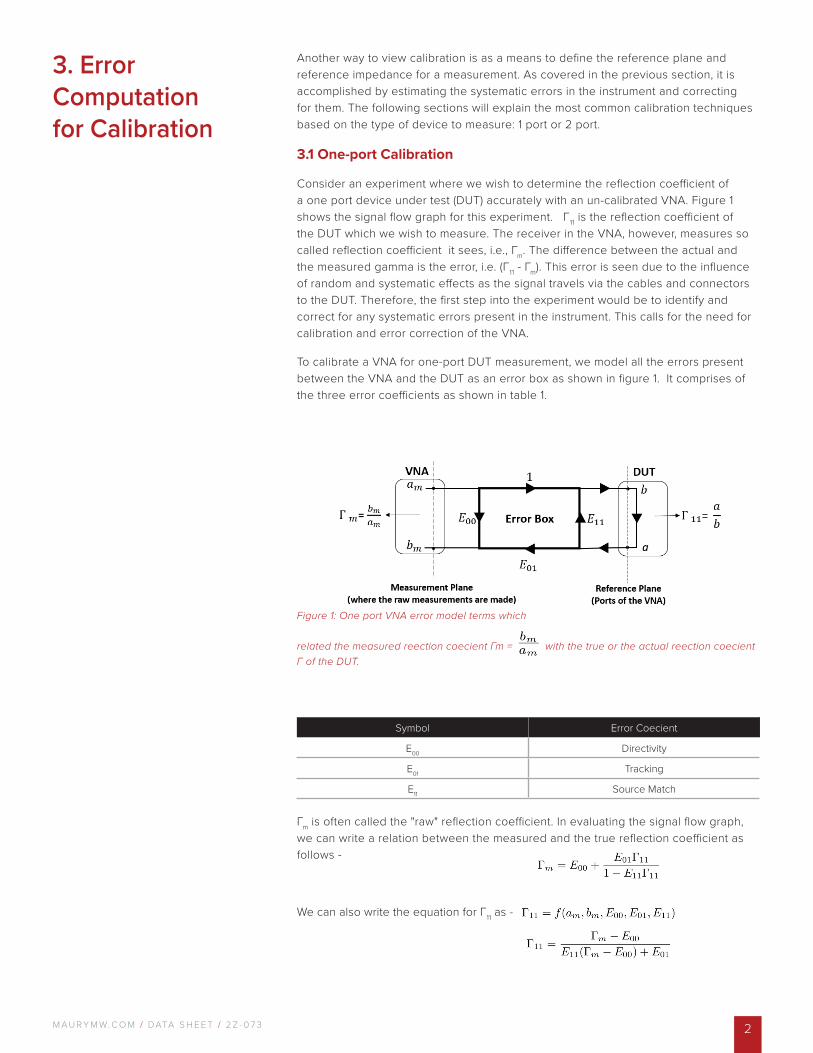
Consider an experiment where we wish to determine the reflection coefficient of a one port device under test (DUT) accurately with an un-calibrated VNA. Figure 1 shows the signal flow graph for this experiment. Γ11 is the reflection coefficient of the DUT which we wish to measure. The receiver in the VNA, however, measures so called reflection coefficient it sees, i.e., Γm. The difference between the actual and the measured gamma is the error, i.e. (Γ11 - Γm). This error is seen due to the influence of random and systematic effects as the signal travels via the cables and connectors to the DUT. Therefore, the first step into the experiment would be to identify and correct for any systematic errors present in the instrument. This calls for the need for calibration and error correction of the VNA.

To calibrate a VNA for one-port DUT measurement, we model all the errors present between the VNA and the DUT as an error box as shown in figure 1. It comprises of the three error coefficients as shown in table 1.

Figure 1: One port VNA error model terms which

related the measured reection coecient Γm = with the true or the actual reection coecient Γ of the DUT.

Γm is often called the "raw" reflection coefficient. In evaluating the signal flow graph, we can write a relation between the measured and the true reflection coefficient as follows -

We can also write the equation for Γ11 as -

Symbol Error Coecient

E00 Directivity

E01 Tracking

E11 Source Match


To find Γ11, we first estimate the error coefficients (by the method of calibration) and then correct for the errors (by the method of error correction). The procedure can be explained as follows -

There are three unknown error terms in eq. (3) namely E00, E01, E11. Thus, we will require at least three equations to solve for them. We begin with three reference standards that we already know the reflection coefficient (Γ11) of. For each standard we can write the eq. 3 where Γm and Γ11 are known, the error terms are the only unknown variables. Using the three standards we get three equations which can be solved to obtain E00, E01, E11 using parametric substitution. Once we know the estimates of the error coefficients from calibration, we can perform error correction for any device under test measurement.

3.2 Two-port Calibration

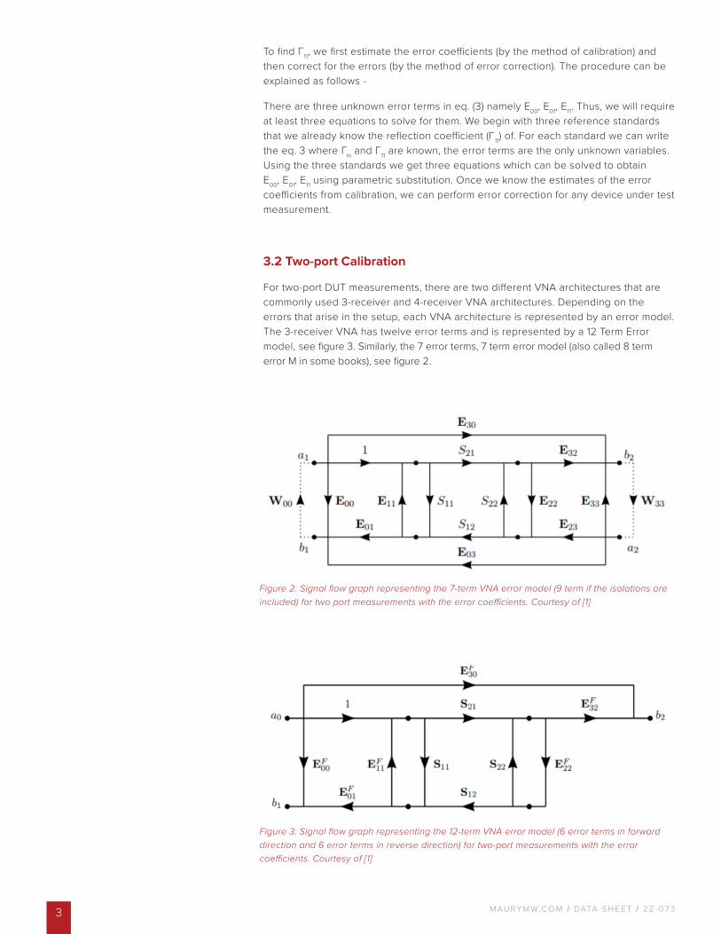
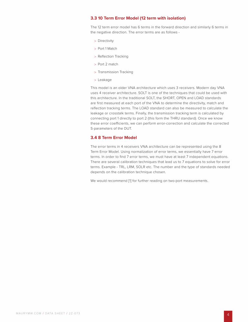
For two-port DUT measurements, there are two different VNA architectures that are commonly used 3-receiver and 4-receiver VNA architectures. Depending on the errors that arise in the setup, each VNA architecture is represented by an error model. The 3-receiver VNA has twelve error terms and is represented by a 12 Term Error model, see figure 3. Similarly, the 7 error terms, 7 term error model (also called 8 term error M in some books), see figure 2.

Figure 2: Signal flow graph representing the 7-term VNA error model (9 term if the isolations are included) for two port measurements with the error coefficients. Courtesy of [1]

Figure 3: Signal flow graph representing the 12-term VNA error model (6 error terms in forward direction and 6 error terms in reverse direction) for two-port measurements with the error coefficients. Courtesy of [1]


3.3 10 Term Error Model (12 term with isolation)

The 12 term error model has 6 terms in the forward direction and similarly 6 terms in the negative direction. The error terms are as follows -

> Directivity

> Port 1 Match

> Reflection Tracking

> Port 2 match

> Transmission Tracking

> Leakage

This model is an older VNA architecture which uses 3 receivers. Modern day VNA uses 4 receiver architecture. SOLT is one of the techniques that could be used with this architecture. In the traditional SOLT, the SHORT, OPEN and LOAD standards are first measured at each port of the VNA to determine the directivity, match and reflection tracking terms. The LOAD standard can also be measured to calculate the leakage or crosstalk terms. Finally, the transmission tracking term is calculated by connecting port 1 directly to port 2 (this form the THRU standard). Once we know these error coefficients, we can perform error-correction and calculate the corrected S-parameters of the DUT.

3.4 8 Term Error Model

The error terms in 4 receivers VNA architecture can be represented using the 8 Term Error Model. Using normalization of error terms, we essentially have 7 error terms. In order to find 7 error terms, we must have at least 7 independent equations. There are several calibration techniques that lead us to 7 equations to solve for error terms. Example - TRL, LRM, SOLR etc. The number and the type of standards needed depends on the calibration technique chosen.

We would recommend [1] for further reading on two-port measurements.


4. Comparison between Existing Techniques

SOLT and TRL are undoubtedly the most commonly used calibration techniques for two port calibration. TRL has the reputation of being a more accurate calibration technique as compared to SOLT even though the math behind SOLT and TRL have the same accuracy.

These two methods dominate the coaxial and waveguide component world. However there are some variations in algorithms frequently used for on wafer measurements. The challenges are not only limited to error computation and characterization, but also extends to the premium real estate available on wafers and ease of probing through automation. We will not cover them in this paper. However the methods discussed here are applicable to on-wafer measurements as well.

The SOLT requires well-defined standards, i.e., well characterized S parameter for each calibration standard - SHORT, OPEN, LOAD and THRU. The two most common methods of defining standards are

Coefficient Model (Polynomial SOLT)

The SOLT calibration requires accurate knowledge of the behavior of the standards. SOLT calibration is only as accurate as the definition of standards used. In practice, however, the standards are approximated by a third degree polynomial function of frequency. This polynomial function is obtained by curve fitting technique which is only an approximation of the true behavior of the standards. The LOAD standards is, moreover, defined by the fixed load model, i.e., the reflection coefficient of the LOAD is assumed to be equal to zero at all frequencies.

Characterized SOLT

When each standard of the SOLT kit is individually and accurately characterized at each frequency point, the calibration is called Characterized SOLT. Each standard in the cal kit is measured for its S parameters and used as the definition of the standard during calibration. Clearly, the standards are more accurately known and there are less assumptions involved. Therefore the accuracy of calibration is enhanced. The challenge is in measuring the standards for accurate definitions.

TRL algorithm inherently requires only approximate characterization of standards - THRU, REFLECT and LINE. Therefore, partial or inaccurate knowledge of the standards does not impact the accuracy of calibration.

We will now look at the comparison of these two techniques.


4.1 TRL Calibration

TRL (Thru-Line-Reflect) calibration procedure requires the measurement of two transmission lines and one reflection standard to determine 2 port - 7 error coefficients (or 9 error coefficients when isolation is included). There are many versions of TRL that use different standards but they are all based on the same error model and its associated assumptions.

Advantages > TRL standards need not be characterized completely. They need to be only partially known. In other words, the accuracy of TRL calibration is independent of how accurately the standards are characterized.

Example When you use a reflect standard for TRL calibration it is sufficient to approximately know what the phase of reflection (if it is greater than -90 degree to less than 90 degree or more than 90 degree to less than 270 degree). The knowledge of the exact exact reflection coefficient of the standard is not required.

> TRL calibration is a common choice for in- fixture and on-wafer environments.

Example For on-wafer measurements with probes it is easier to manufacture and partially characterize 3 TRL standards as opposed to four in case of SOLT.

Disadvantages > The airlines used in TRL coax kits, are beadless thus the center conductor is movable. This gives rise to the following repeatability problems -

1. By virtue of how these are connected to the test ports, one side always has close to zero pin depth and the other side has some amount pin depth, neither of which are repeatable with multiple measurements.

2. The center conductor may not be perfectly.

3. It requires some experience or skills to connect TRL standards in a repeatable manner especially as the connectors become smaller at high frequencies.

> The major limitation of the TRL technique is the limited bandwidth of LINE standards. For broadband measurements several line standards may be required, thus making the calibration more complicated and time consuming.

Example A span from 2 GHz to 26 GHz requires 2 line standards.

> TRL calibration is not accurate if the reflect standards connected at the two ports is not same.

> The characteristic impedance of the LINE and THRU implicitly defines the characteristic impedance of measurement. Therefore, all lines must have the same characteristic impedance as the impedance at which the user desires to calibrate.

Why do we require multiple airline standards of varying length for TRL?

The math that supports TRL breaks down if the line standard is 0° or 180° in length. Therefore, a safe limit of the length of the airline is considered to be between 20° and 160° of the wave rotation or 8:1 bandwidth. This means that if a line standard is 20° in length at 1 GHz, the maximum frequency it can be used up to is 8 GHz. To calibrate for frequency beyond 8 GHz you would require another line standard.


> At low frequencies the LINE standard becomes too long for practical use. Since the airlines are not beaded, there is nothing to hold the center conductor in the center and it tends to bend due to gravity. This changes the characteristic impedance of the airline.

> Similarly, at high frequency the LINE standard becomes too short. Since the connectors have a fixed minimum length and the length LINE includes the length of the connectors, this sets the lower limit to how short the airline can be manufactured.

> TRL calibration may not be suitable for measurement setups where the distance between the reference plane is fixed. This is due to the fact that TRL requires different lengths of THRU and LINE.

> TRL standards can only be used for two port calibration.

>

4.2 Polynomial SOLT Calibration

The traditional SOLT two port VNA calibration requires the knowledge of 4 standards namely the Short, Open, Load and Thru to solve for error coefficients of the 10 error term model (or 12 if isolation error is included). The calibration corrects for error due to directivity, isolation, source match and reflection and transmission tracking in both forward and reverse directions.

Advantages > SOLT standards are beaded and therefore easy to connect.

> It is an added advantage that a subset of the SOLT kit can be used to do a one port calibration, i.e., SOL with no additional requirements.

> SOLT inherently provides a broadband calibration, essentially from DC to the upper frequency limit of the connector type being used.

Disadvantages > The fundamental limitation of the SOLT calibration algorithm is that all of the standards must have fully known electrical behavior.

> The accuracy of the SOLT calibration is limited by how accurately you know the standards or how well the standards are characterized.

> Polynomial SOLT kit standards are characterized by the same polynomial function which is only an approximation of the actual behavior of the standard.


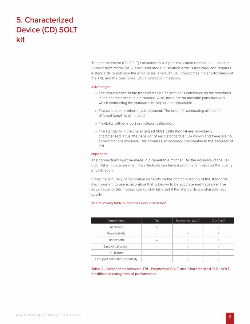
The characterized (CD SOLT) calibration is a 2 port calibration technique. It uses the 10 error term model (or 12 error term model if isolation error is included) and requires 4 standards to estimate the error terms. The CD SOLT overcomes the shortcomings of the TRL and the polynomial SOLT calibration methods.

Advantages > The convenience of the traditional SOLT calibration is conserved as the standards in the characterized kit are beaded. Also, there are no movable parts involved which connecting the standards is simpler and repeatable.

> The calibration is inherently broadband. The need for connecting airlines of different length is eliminated.

> Flexibility with one port or multiport calibration.

> The standards in the characterized SOLT calibration kit are individually characterized. Thus, the behavior of each standard is fully known and there are no approximations involved. This promises an accuracy comparable to the accuracy of TRL.

Important:

The connections must be made in a repeatable manner. As the accuracy of the CD SOLT kit is high, even small imperfections can have a prominent impact on the quality of calibration.

Since the accuracy of calibration depends on the characterization of the standards, it is important to use a calibration that is known to be accurate and traceable. The advantages of this method can quickly fall apart if the standards are characterized poorly.

The following table summarizes our discussion.

Table 2: Comparison between TRL, Polynomial SOLT and Characterized "CD" SOLT for different categories of performance.

5. Characterized Device (CD) SOLT kit

Performance TRL Polynomial SOLT CD SOLT

Accuracy ✓ - +

Repeatability - + +

Bandwidth - + +

Ease of calibration - + +

In- fixture + + +

One port calibration capability - + +


6. Experimental Study on Accuracy

6.1 What are Residual Errors?

Perfect calibration of a VNA is improbable in the real world due to sources of uncertainty such as non-linearity, VNA drift and noise, cable stability, connection repeatability etc. The quality of calibration is also limited by the accuracy of characterization of the standards used.

Is there a way we could estimate how good our calibration is? Or can we estimate how much error is remaining in our measurement system after calibration? This brings us to the topic of verification of calibration. And this is done traditionally by measuring residual errors. Residual error, as the name suggests, is the error remaining in the measurement equipment

after it has been calibrated. The more accurately we calibrate, the residual errors are the measuring equipment. The methods for estimating the error terms are the ripple method and Time Domain Reflectometery(TDR).

The residual error in directivity is called effective directivity or δE00. Similarly, the other residual error terms are effective tracking or δE01 and effective source match or δE11.

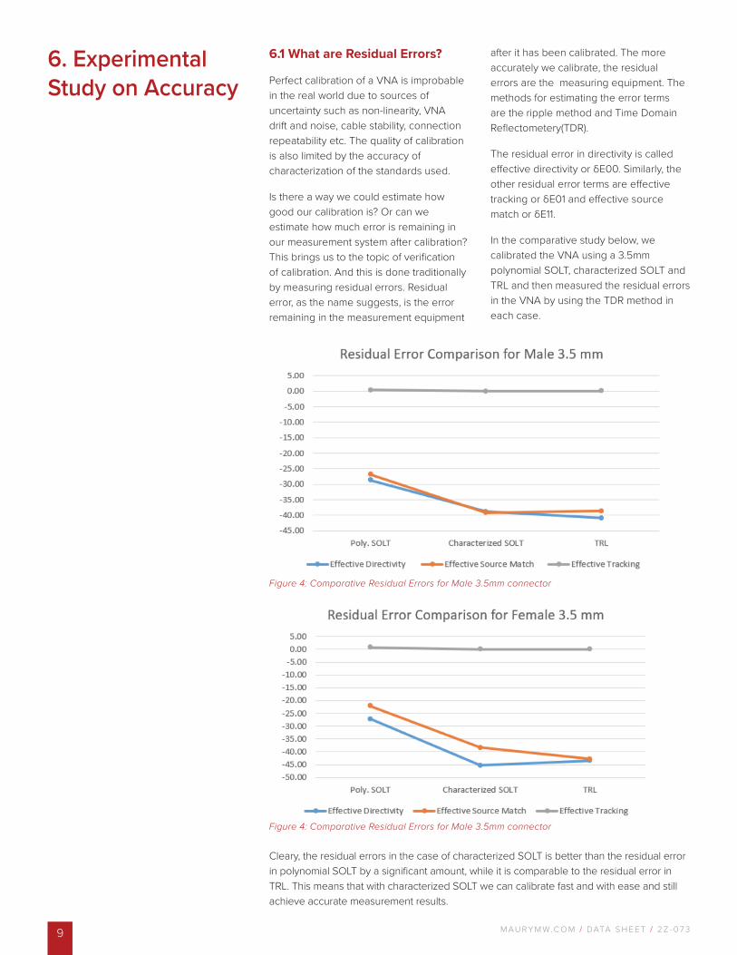
In the comparative study below, we calibrated the VNA using a 3.5mm polynomial SOLT, characterized SOLT and TRL and then measured the residual errors in the VNA by using the TDR method in each case.

Figure 4: Comparative Residual Errors for Male 3.5mm connector

Figure 4: Comparative Residual Errors for Male 3.5mm connector

Cleary, the residual errors in the case of characterized SOLT is better than the residual error in polynomial SOLT by a significant amount, while it is comparable to the residual error in TRL. This means that with characterized SOLT we can calibrate fast and with ease and still achieve accurate measurement results.


[1] Guidelines on the evaluation of vector network analyzers (VNA), https://www.euramet.org/Media/news/I-CAL-GUI-012_Calibration_ Guide_No._12.web.pdf

[2] G. F. Engen and C. A. Hoer, Thru-reflect-line: An improved technique for calibrating the dual six-port automatic network analyzer, IEEE Transactions on Microwave Theory and Techniques, vol. 27, no. 12, pp. 987 993, Dec 1979.

[3] "Using simple calibration load models to improve accuracy of vector network analyser measurements", Nick Ridler, Nils Nazoa, 67th Automatic RF Techniques Group (ARFTG) conference digest, pp 104-110, San Francisco, California, USA, 16 June 2006. (https://ridler-pubs.webs.com/NMR_123.pdf)

[4] LRL calibration of Vector Network Analyzers. Maury app note 5A-017 https://www.maurymw.com/pdf/datasheets/5A-017.pdf

[5] Verifying the performance of Vector Network Analyzer. Maury app note 5C-026 https://www.maurymw.com/pdf/datasheets/5C-026.pdf

[6] Ferrero, A. (2013). Two-port network analyzer calibration. In V. Teppati, A. Ferrero, & M. Sayed (Eds.), Modern RF and Microwave Measurement Techniques (The Cambridge RF and Microwave Engineering Series, pp. 195-218). Cambridge: Cambridge University Press. doi:10.1017/CBO9781139567626.009

References

V I S I T O U R W E B S T O R E

T O L E A R N M O R E A B O U T

O U R P R O D U C T S

w w w . m a u r y m w . c o m____

C O N TAC T U S :W / maurymw.comE / [email protected] / +1-909-987-4715 F / +1-909-987-11122900 Inland Empire BlvdOntario, CA 91764

A P P L I C AT I O N N OT E / 5 C - 0 9 0© 2019 Maury Microwave Corporation. All Rights Reserved.Specifications are subject to change without notice.Maury Microwave is AS9100D & ISO 9001:2015 Certified.

Improving Calibration Accuracy and Speed with ... · Accuracy and Speed with Characterized...

Documents

Transcript of Improving Calibration Accuracy and Speed with ... · Accuracy and Speed with Characterized...