MIT LIBRARIES DEWEY.

3 9080 02898 1451

Massachusetts Institute of Technology

Department of EconomicsWorking Paper Series

IMPROVING POINT AND INTERVAL ESTIMATES OFMONOTONE FUNCTIONS BY REARRANGEMENT

Victor Chernozhukov

Ivan Fernandez-Val

Alfred Galichon

Working Paper 08-1

3

July 2, 2008

Room E52-251

50 Memorial Drive

Cambridge, MA 02142

This paper can be downloaded without charge from the

Social Science Research Network Paper Collection at

http://ssrn com/abstract=1 1 59965

Digitized by the Internet Archive

in 2011 with funding from

Boston Library Consortium IVIember Libraries

http://www.archive.org/details/improvingpointinOOcher

IMPROVING POINT AND INTERVAL ESTIMATES OF MONOTONEFUNCTIONS BY REARRANGEMENT

VICTOR CHERNOZHUKOV' IVAN FERNANDEZ-VAL* ALFRED GALICHON'

Abstract. Suppose that a target function fo : M.'' —* R is monotonic, namely weakly in-

creasing, and an original estimate / of this target function is available, which is not weakly

increasing. Many common estimation methods used in statistics produce such estimates /.

We show that these estimates can always be improved with no harm by using rearrangement

techniques: The rearrangement methods, univariate and multivariate, transform the original

estimate to a monotonic estimate /', and the resulting estimate is closer to the true curve /o

in common metrics than the original estimate /. The improvement property of the rearrange-

ment also extends to the construction of confidence bands for monotone functions. Let ( and

u be the lower and upper endpoint functions of a simultaneous confidence interval [(,u] that

covers /o with probability 1 — q, then the rearranged confidence interval [^',u'), defined by

the rearranged lower and upper end-point functions (' and u' , is shorter in length in common

norms than the original interval and covers /o with probability greater or equal to 1 - q. Weillustrate the results with a computational example and an empirical example dealing with

age-height growth charts.

Key words. Monotone function, improved estimation, improved inference, multivariate re-

arrangement, univariate rearrangement, Lorentz inequalities, growth chart, quantile regres-

sion, mean regression, series, locally linear, kernel methods

AMS Subject Classification. Primary 62G08; Secondary 46F10, 62F35, 62P10

Date: First version is of December, 2006- Two ArXiv versions of paper arc available, ArXiv 0704.3686 (April, 2007) and

ArXiv: 0806 4730 (June, 2008) This version is of July 2, 200S. The previous title of this paper was "Improving Estimates of

Monotone Functions by Rearrangement". Wp would like to thank the editor, the associate editor, the anonymous referees of

the journal, Richard Blundell, Eric Cator, Andrew Chcshcr, Moshc Cohen, Holgor Dettc. Emily Gallagher, Pict Groeneboom,

Raymond Guiteras, Xuming He, Roger Koenkcr, Charles Manski, Costas Meghir, Ilya Molchanov, Whitney Newey, Steve Port-

noy. Alp Simsek, Jon Wellner and seminar participants at BU, CEMFI, CEMMAP Measurement Matters Conference, Columbia,

Columbia Conference on Optimal Transportation, Conference Frontiers of Microeconomctrics in Tokyo, Cornell, Cowless Founda-

tion 75th Anniversary Conference. Duke- Triangle, Georgetown, MIT. MIT-Harvard, Northwestern, UBC, UCL, UIUC. University

of Alicante. University of Gothenburg Conference "Nonsmooth Inference, Analysis, and Dependence," and Yale University for

very useful comments that helped to considerably improve the paper.

Massachusetts Institute of Technology, Department of Economics &: Operations Research Center, and University College

London, CEMMAP. E-maii: vchern@mit.edu. Research support from the Castle Krob Chair, National Science Foundation, the

Sloan Foundation, and CEMMAP is gratefully acknowledged

§ Boston University, Department of Economics. E-mail: ivafif@bii,edii, Re.search support from the National Science Founda-

tion is gratefully acknowledged,

J Ecole Polytechniquc, Departement d'Economie, E-mail: alfred.galichon@polytechnique edu.

1

,1. Introduction •

A common problem in statistics is the approximation of an unknown monotonic function

using an available sample. There are many examples of monotonically increasing functions,

including biometric age-height charts, which should be monotonic in age; econometric de-

mand functions, which should be monotonic in price; and quantile functions, which should

be monotonic in the probability index. Suppose an original, potentially non-monotonic, esti-

mate is available. Then, the rearrangement operation from variational analysis (Hardy, Lit-

tlewood, and Polya 1952, Lorentz 1953, Villani 2003) can be used to monotonize the orig-

inal estimate. The rearrangement has been shown to be useful in producing monotonized

estimates of density functions (Fougeres 1997), conditional mean functions (Davydov and

Zitikis 2005, Dette, Neumeyer, and Pilz 2006, Dette and Pilz 2006, Dette and Scheder 2006),

and various conditional quantile and distribution functions (Chernozhukov, Fernandez- Val,

and Galichon (2006b, 2006c)).

In this paper, we show, using Lorentz inequalities and their appropriate generalizations,

that the rearrangement of the original estimate is not only useful for producing monotonicity,

but also has the following important property: The rearrangement always improves upon the

original estimate, whenever the latter is not monotonic. Namely, the rearranged curves are

always closer (often considerably closer) to the target curve being estimated. Furthermore,

this improvement property is generic, i.e., it does not depend on the underlying specifics of

the original estimate and applies to both univariate and multivariate cases. The improvement

property of the rearrangement also extends to the construction of confidence bands for mono-

tone functions. We show that we can increase the coverage probabilities and reduce the lengths

of the confidence bands for monotone functions by rearranging the upper and lower bounds of

the confidence bands.

Monotonization procedures have a long history in the statistical literature, mostly in relation

to isotone regression. While we will not provide an extensive literature review, we reference the

methods other than rearrangement that are most related to the present paper. Mammen (1991)

studies the effect of smoothing on monotonization by isotone regression. He considers two

alternative two-step procedures that differ in the ordering of the smoothing and monotonization

steps. The resulting estimators are asymptotically equivalent up to first order if an optimal

bandwidth choice is used in the smoothing step. Mammen, Marron, Turlach, and Wand (2001)

show that most smoothing problems, notably including smoothed isotone regression problems,

can be recast as a projection problem with respect to a given norm. Another approach is the

one-step procedure of Ramsay (1988), which projects on a class of monotone spline functions

called I-splines. Later in the paper we will make both analytical and numerical comparisons

of these procedures with the rearrangement.

2. Improving Point Estimates of Monotone Functions by Rearrangement

2.1. Common Estimates of Monotonia Functions. A basic problem in many areas of

statistics is the estimation of an unknown function /o : M'' ^ R using the available information.

Suppose we know that the target function /o is monotonia, namely weakly increasing. Suppose

further that an original estimate / is available, which is not necessarily monotonic. Many

common estimation methods do indeed produce such estimates. Can these estimates always

be improved with no harm? The answer provided by this paper is yes: the rearrangement

method transforms the original estimate to a monotonic estimate /*. and this estimate is in

fact closer to the true curve /b than the original estimate / in common metrics. Furthermore,

the rearrangement is computationally tractable, and thus preserves the computational appeal

of the original estimates.

Estimation methods, specifically the ones used in regression analysis, can be grouped into

global methods and local methods. An example of a global method is the series estimator of

/o taking the form ' • \-.

" -; ,: ,- , : - ., ; .

;

where Pk„{x) is a fc„-vector of suitable transformations of the variable x, such as B-splines,

polynomials, and trigonometric functions. Section 4 lists specific examples in the context of

an empirical example. The estimate b is obtained by solving the regression problem

n

b = a.Tg min y"p{Y, - Pk„{X,yb), \1=1

where {Yi,Xi),i = l,...,n denotes the data. In particular, using the square loss p{u) = v?

produces estimates of the conditional mean of Yi given X,; (Gallant 1981, Andrews 1991, Stone

1994, Newey 1997), while using the asymmetric absolute deviation loss p{u) = (u — l(u < 0))u

produces estimates of the conditional u-quantile of Y, given Xi (Koenker and Bassett 1978,

Portnoy 1997, He and Shao 2000). The series estimates x ^-^ f{x) = Pk„ {x)'b are widely used in

data analysis due to their desirable approximation properties and computational tractability.

However, these estimates need not be naturally monotone, unless explicit constraints are added

into the optimization program (see, for example, Matzkin (1994), Silvapulle and Sen (2005),

and Koenker and Ng (2005)).

Examples of local methods include kernel and locally polynomial estimators. A kernel

estimator takes the form

/(i) = argmin S" Wrp{Y^ - 6), u^ = K [ —^1=1 ^

where the loss function p plays the same role as above, K{u) is a standard, possibly high-order,

kernel function, and ^ > is a vector of bandwidths (see, for example, Wand and Jones (1995)

and Ramsay and Silverman (2005)). The resulting estimate x i-* /(x) need not be naturally

monotone. Dette, Neumeyer, and Pilz (2006) show that the rearrangement transforms the

kernel estimate into a monotonic one. We further show here that the rearranged estimate

necessarily improves upon the original estimate, whenever the latter is not monotonic. The

locally polynomial regression is a related local method (Chaudhuri 1991, Fan and Gijbels 1996).

In particular, the locally linear estimator takes the form

{f{x),d{x)) = argmin Y] Wip{Yi -b~ d{X, - x)f, w, = K [^-—

6eR,deR ~l V "

The resulting estimate x i—> f{x) may also be non-monotonic, unless explicit constrains are

added to the optimization problem. Section 4 illustrates the non-monotonicity of the locally

linear estimate in an empirical example.

In summary, there are many attractive estimation and approximation methods in statistics

that do not necessarily produce monotonic estimates. These estimates do have other attractive

features though, such as good approximation properties and computational tractability. Below

we show that the rearrangement operation applied to these estimates produces (monotonic)

estimates that improve the approximation properties of the original estimates by bringing them

closer to the target curve. Furthermore, the rearrangement is computationally tractable, and

thus preserves the computational appeal of the original estimates.

2.2. The Rearrangement and its Approximation Property: The Univariate Case.

In what follows, let ,^ be a compact interval. Without loss of generality, it is convenient to

take this interval to be ,^ = [Oil]- Let f{x) be a measurable function mapping X to K, a

bounded subset of R. Let Ff{y) = j-^ l{f{u) < y}du denote the distribution function of f(X)

when X follows the uniform distribution on [0, 1]. Let

r{x):=Qf{x):=inf{yeR:Ff{y)>x}

be the quantile function of Fj{y). Thus, .

r{x) :=inf Ue / l{f{u) < y}duJx

> Xix

This function /* is called the increasing rearrangement of the function /.

Thus, the rearrangement operator simply transforms a function / to its quantile function /*.

That is, X i—> f*{x) is the quantile function of the random variable f{X) when X ~ L/(0, 1).

It is also convenient to think of the rearrangement as a sorting operation: given values of the

function /(,r) evaluated at i in a fine enough net of equidistant points, we simply sort the

values in an increasing order. The function created in this way is the rearrangement of /.

The first main point of this paper is the following:

Proposition 1. Let fo : X ^' K be a weakly increasing measurable function in x. This is

the target function. Let f : X -^ K he another measurable function, an initial estimate of the

target function /o-

L For any p € [1, oo], the rearrangement of f , denoted /*, weakly reduces the estimation error:

Xrix)-fo{x) dx

i/p

<I f{x)-JX

Mx]ll/p

dx (2.1)

2. Suppose that there exist regions Xq and Xq, each of measure greater than 5 > Q, such

that for all x £ Xo and x' S Xq we have that (i) x' > x, (ii) f{x) > f(x') + e, and (Hi)

/o(x') > fo{x) + e, for some e > 0. Then the gam in the quality of approximation is strict for

p £ (l.co). Namely, for any p G (1,(X)),

Xr(x)-fo{x) dx

i/p

< \f{x) - fo{x) dx - 5nIX

i/p

(2.2)

where rjp = inf{|D — t'\^ + \v' — i|f — \v - t^ — \v' — t'\^} > 0, with the infimum taken over all

v,v' ,t, t' in the set K such that v' > v + e and t' > t + e.

This proposition establishes that the rearranged estimate /* has a smaller (and often strictly

smaller) estimation error in the Lp norm than the original estimate whenever the latter is not

monotone. This is a very useful and generally applicable property that is independent of the

sample size and of the way the original estimate / is obtained. The first part of the proposition

states the weak inequality (2.1), and the second part states the strict inequality (2.2). For

example, the inequality is strict for p £ (1,00) if the original estimate f{x) is decreasing on

a subset of X having positive measure, while the target function fo{x) is increasing on X (by

increasing, we mean strictly increasing throughout). Of course, if fo{x) is constant, then the

inequality (2.1) becomes an equality, as the distribution of the rearranged function /* is the

same as the distribution of the original function /, that is F;, = Ff fThe weak inequality (2.1) is a direct (yet important) consequence of the classical rearrange-

ment inequality due to Lorentz (1953): Let q and g be two functions mapping X to K. Let q*

and g* denote their corresponding increasing rearrangements. Then,

L{q*{x),g*{x))dx < / L{q{x),g{x))dx, ' .'

.•:;

X Jx

for any submodular discrepancy function L : R^ ^-> E+. Set q{x) = f{x), q*{x) = f*{x),

g{x) = /o(x), and g*{x) = foix). Now, note that in our case /q (a;) = /o(2;) almost everywhere,

that is, the target function is its own rearrangement. Let us recall that L is submodular if for

each pair of vectors {v,v') and (t,t') in R^,' we have that .

L{v Av',t/\ t') + L(y \J v',t\J t') < L{v, t) + L(y' , t'), (2.3)

In other words, a function L measuring the discrepancy between vectors is submodular if

co-monotonization of vectors reduces the discrepancy. When a function L is smooth, submod-

ularity is equivalent to the condition dvdtL{v,t) < holding for each {v,t) in IR^. Thus, for

example, power functions L{v,t) = \v — t\^ for p £ [l,oo) and many other loss functions are

submodular.

In the Appendix, we provide a proof of the strong inequality (2.2) as well as the direct proof

of the weak inequality (2.1). The direct proof illustrates how reductions of the estimation error

arise from even a partial sorting of the values of the estimate /. Moreover, the direct proof

characterizes the conditions for the strict reduction of the estimation error.

It is also worth emphasizing the following immediate asymptotic implication of the above

finite-sample result: The rearranged estimate /* inherits the L-p rates of convergence from the

original estimates /. For p e [l,c»], if A,, =[/:^. 1/(3:) - /o(x)|''du]^'''' = Op{aTi) for some

sequence of constants On, then [J^ \I*{'^) — fo{x)\^duY/^ < A„ = Op[an)-

2.3. Computation of the Rearranged Estimate. One of the following methods can be

used for computing the rearrangement. Let {Xj.'j = 1 B] be either (1) a set of equidistant

points in [0, 1] or (2) a sample of i.i.d. draws from the uniform distribution on [0, 1]. Then the

rearranged estimate f*{u) at point u € X can be approximately computed as the u-quantile

of the sample {f{Xj),i = 1,...,S}. The first method is deterministic, and the second is

stochastic. Thus, for a given number of draws B, the complexity of computing the rearranged

estimate /*(u) in this way is equivalent to the complexity of computing the sample u-quantile

in a sample of size B. The number of evaluations B can depend on the problem. Suppose

that the density function of the random variable f{X), when A' ^ U{0, 1), is bounded away

from zero over a neighborhood of f*{x). Then f*{x) can be computed with the accuracy of

Op(l/-\/S), as B ^ oo, where the rate follows from the results of Knight (2002).

2.4. The Rearrangement and Its Approximation Property: The Multivariate Case.

In this section we consider multivariate functions / ; X'^ —> K, where A''' = [0, l]"^ and K is

a bounded subset of K. The notion of monotonicity we seek to impose on / is the following:

We say that the function / is weakly increasing in x if f{x') > f{x) whenever ,r' > x. The

notation x' = {x\,...,x'^) > a; = {x],...,Xd) means that one vector is weakly larger than the

other in each of the components, that is, i' > Xj for each j = 1 d. In what follows, we

use the notation f{xj,x^j) to denote the dependence of / on its j-th argument, ij, and all

other arguments, :r_j, that exclude Xj. The notion of monotonicit}' above is equivalent to the

requirement that for each j in 1, ...,d the mapping Xj i—> /(xj,x_j) is weakly increasing in x_,,

for each x_j in X'^~^

.

Define the rearranged operator Rj and the rearranged function fj{x) with respect to the

j-th argument as follows:

f;ix):=Rjof{x):=\nnyJ

l{f{x'^,x.j)<y}dx'^ >xAUx

This is the one-dimensional increasing rearrangement applied to the one-dimensional function

Xj I—> f{Xj,X-j), holding the other arguments x^j fixed. The rearrangement is applied for

every value of the other arguments x_j.

Let TT = (tti, .... TTd) be an ordering, i.e., a permutation, of the integers 1, ...,d. Let us define

the TT-rearrangement operator R^ and the 7r-rearranged function f*{x) as follows:

f:{x):=R^of{x):=R^,o...oR,^of{x).

For any ordering tt, the 7r-reaxrangement operator rearranges the function with respect to all

of its arguments. As shown below, the resulting function /^(a;) is weakly increasing in x.

In general, two different orderings tt and n' of 1, ...,d can yield different rearranged functions

/*(a;) and f*,{x). Therefore, to resolve the conflict among rearrangements done with different

orderings, we may consider averaging among them: letting 11 be any collection of distinct

orderings tt, we can define the average rearrangement as

' ' Tren

where |n[ denotes the number of elements in the set of orderings 11. Dette and Scheder (2006)

also proposed avera.ging all the possible orderings of the smoothed rearrangement in the context

of monotone conditional mean estimation. As shown below, the approximation error of the

average rearrangement is weakly smaller than the average of approximation errors of individual

TT-rearrangements. '..'', . -.,

The following proposition describes the properties of multivariate yr-rearrangements;

Proposition 2. Let the target function /o : X"^ -^ K be weakly increasing and measurable in x.

Let f : X —* K be a measurable function that is an initial estimate of the target function /q.

Let f : X'^ —' K be another estimate of fo, which is measurable in x, including, for example,

a rearranged f with respect to some of the arguments. Then,

1. For each ordering n of 1, ..., d, the tt -rearranged estimate f^{x) is weakly increasing in x.

Moreover, f*{x), an average of tt -rearranged estimates, is weakly increasing in x.

2. (a) For any j in 1, ...,d and any p in [l,oo], the rearrangement of f with respect to the

j-th argument produces a weak reduction in the approximation error:

\f;ix)-fo{x)\PdxX"

1/p

<1/p

\f{x) - fo{xWdx\ . (2.5)

X''

(b) Consequently, a -n -rearranged estimate f^{x) of f{x) weakly reduces the approximation

error of the original estimate:

l/;(x) - fo{x)\PdxUX"

1/p

Ux-'\f{x) - foixWdx

-ii/p

(2.6)

3. Suppose that f{x) and /o(x) have the following properties: there exist subsets Xj c Xand A"' C X , each of measure 5 > 0, and a subset X-j C X , of measure v > Q, such that

for all x = {xj,X-j) and x' = (a;',a;_j), with x' G X'^ Xj £ Xj, X-j G X-j, we have that (i)

x'j > Xj, (a) f{x) > f{x') + e, and (lii) fo{x') > fo{x) + e, for some e > 0.

(a) Then, for any p € (1, oo),

\f;(x)-fo{x)\pdx

1/p

X''

\f{x) - fo{x)\Pdx - ripSiy

i/p

(2.7)

where rjp = inf{|D — i'jP + \v' — tp — \v - t\P — \v' - t'\P} > 0, with the mfimum. taken over all

V, v', t, t' in the set K such that v' > v + e and t' > t + e.

(b) Further, for an ordering tt = (tti, ..., tt;,.. ••i "'rf) with -Kk = j, 'e^ f be a partially rearranged

function, f(x) = Rtt^^^ ° o R-n^ ° f{x) (for k = d we set f{x) = f{x)). If the function f[x)

and the target function fo{x) satisfy the condition stated above, then, for any p £ (l,oo),

Ux-i\f:(x) - fo{x)\^dx

ii/p

<Ix-i

\f{x)-fo{x)rdx-iipSuTl/P

4- The approximation error of an average rearrangement is weakly smaller than the average

approximation error of the individual tt- rearrangements: For any p G [l,oo],

Ix-i\rix)^foix)\^dx

1/p

in!T̂ren Ux''

\rAx) - fo{x)\Pdx

1/p

(2.9)

This proposition generalizes the results of Proposition 1 to the multivariate case, also demon-

strating several features unique of the multivariate case. We see that the 7r-rearranged functions

are monotonic in all of the arguments. Dette and Scheder (2006), using a different argument,

showed that their smoothed rearrangement for conditional mean functions is monotonic in

both arguments for the bivariate case in large samples. The rearrangement along any argu-

ment improves the approximation properties of the estimate. Moreover, the improvement is

strict when the rearrangement with respect to a j-th argument is performed on an estimate

that is decreasing in the j-th argument, while the target function is increasing in the same

j-th argument, in the sense precisely defined in the proposition. Moreover, averaging different

TT-rearrangements is better (on average) than using a single tt- rearrangement chosen at random.

All other basic implications of the proposition are similar to those discussed for the univariate

case.

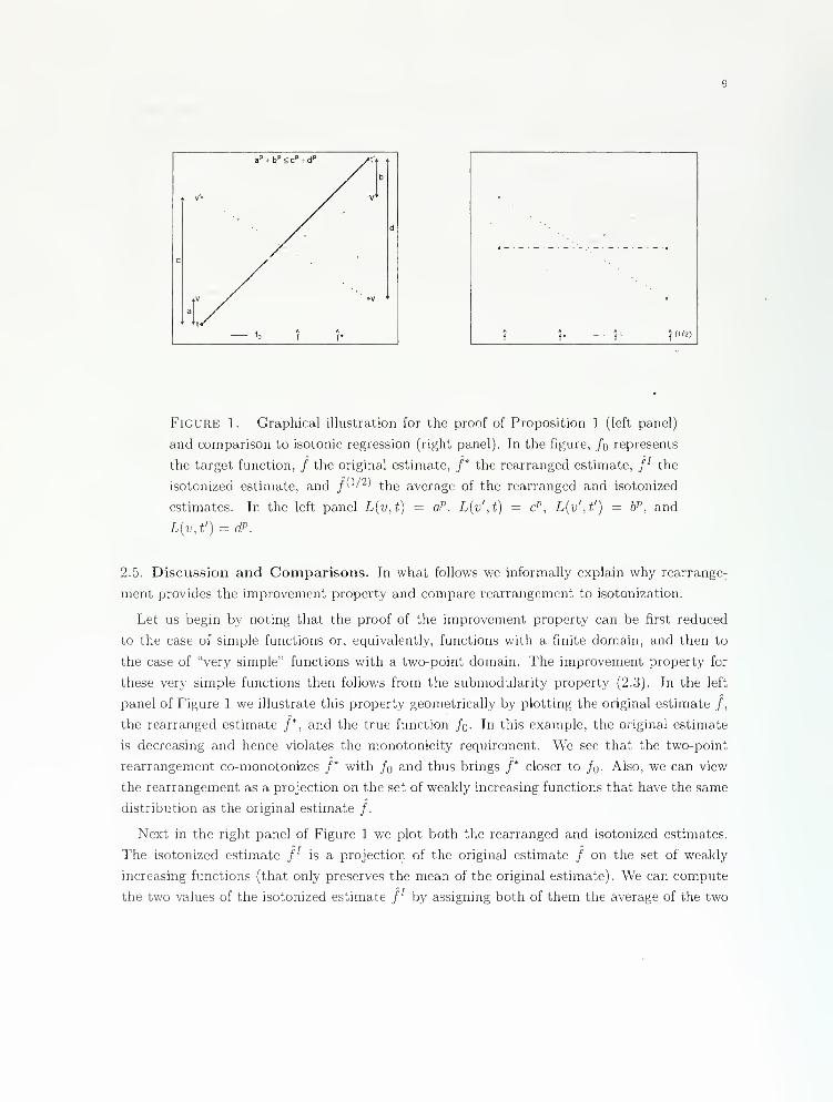
Figure 1. Graphical illustration for the proof of Proposition 1 (left panel)

and comparison to isotonic regression (right panel). In the figure, /o represents

the target function, / the original estimate, /* the rearranged estimate, f' the

isotonized estimate, and /'''^' the average of the rearranged and isotonized

estimates. In the left panel L{v,t) = oP, L{v\t) ~ d', L{v',t') = b^, and

L{v,t') = dP.

2.5. Discussion and Comparisons. In what follows we informally explain why rearrange-

ment provides the improvement property and compare rearrangement to isotonization.

Let us begin by noting that the proof of the improvement property can be first reduced

to the case of simple functions or, equivalently, functions with a finite domain, and then to

the case of "very simple" functions with a two-point domain. The improvement property for

these very simple functions then follows from the submodularity property (2.3). In the left

panel of Figure 1 we illustrate this property geometrically by plotting the original estimate /,

the rearranged estimate /*, and the true function /q. In this example, the original estimate

is decreasing and hence violates the monotonicity requirement. We see that the two-point

rearrangement co-monotonizes /* with /o and thus brings /* closer to Jq. Also, we can view

the rearrangement as a projection on the set of weakly increasing functions that have the same

distribution as the original estimate /•, . ,

'

,, .

Next in the right panel of Figure 1 we plot both the rearranged and isotonized estimates.

The isotonized estimate /^ is a projection of the original estimate / on the set of weakly

increasing functions (that only preserves the mean of the original estimate). We can compute

the two values of the isotonized estimate y by assigning both of them the average of the two

10

values of the original estimate /, whenever the latter violate the monotonicity requirement, and

leaving the original values unchanged, otherwise. We see from Figure 1 that in our example

this produces a flat function /^. This computational procedure, known as "pool adjacent

violators," naturally extends to domains with more than two points by simply applying the

procedure iteratively to any pair of points at which the monotonicity requirement remains

violated (Ayer, Brunk, Ewing, Reid, and Silverman 1955).

Using the computational definition of isotonization, one can show that, like rearrangement,

isotonization also improves upon the original estimate, for any p € [l,oo]:

\f'{x)-Mx)\^dx1/p

< \f{x)-Mx)\Pdxll/p

(2.10)

see, e.g.. Barlow, Bartholomew, Bremner, and Brunk (1972). Therefore, it follows that any

function f^ in the convex hull of the rearranged and the isotonized estimate both monotonizes

and improves upon the original estimate. The first property is obvious and the second follows

from homogeneity and subadditivity of norms, that is for any p £ [l,oo]:

\f Mx)\''dxUp

< A \f\x)~h{x)Y'dx

i/p

+ (1-A) ir(.r)-/o(2)Rx

i/p

l/(-r) - h{x)ydxi/p

(2.11)

where f^{x) = \f*{x) + (1 — X)f' (x) for any A £ [0, 1]. Before proceeding further, let us also

note that, by an induction argument similar to that presented in the previous section, the

improvement property listed above extends to the sequential multivariate isotonization and to

its convex hull with the sequential multivariate rearrangement.

Thus, we see that a rather rich class of procedures (or operators) both monotonizes the

original estimate and reduces the distance to the true target function. It is also important to

note that there is no single best distance-reducing monotonizing procedure. Indeed, whether

the rearranged estimate /* approximates the target function better than the isotonized estimate

f^ depends on how steep or flat the target function is. We illustrate this point via a simple

example plotted in the right panel of Figure 1; Consider any increasing target function taking

values in the shaded area between /* and /^, and also the function /^Z"^, the average of the

isotonized and the rearranged estimate, that passes through the middle of the shaded area.

Suppose first that the target function is steeper than /^'^, then /* has a smaller approximation

error than /'. Now suppose instead that the target function is flatter than /'Z^, then f^ has

a smaller approximation error than /*. It is also clear that, if the target function is neither

very steep nor very flat, /^^^ can outperform either /* or /''. Thus, in practice we can choose

rearrangement, isotonization, or, some combination of the two, depending on our beliefs about

how steep or flat the target function is in a particular application.

11

3. Improving Interval Estimates of Monotone Functions by Rearrangement

In this section we propose to directly apply the rearrangement, univariate and multivariate,

to simultaneous confidence intervals for functions. We show that our proposal will necessarily

improve the original intervals by decreasing their length and increasing their coverage.

Suppose that we are given an initial simultaneous confidence interval

\£,u]^{\e{x),u{x)],xeX''), (3.1)

where i{x) and u{x) are the lower and upper end-point functions such that i{x) < u{x) for all

X £ X<^.

We further suppose that the confidence interval [i, u] has either the exact or the asymptotic

confidence property for the estimand function /, namely, for a given a G (0, 1),

Probp{/ € \t,u]] = Probp{£(a;) < J{x) < u{x), for all x e X'^} > I - a, (3.2)

for all probabihty measures P in some set Vn containing the true probability measure Pg. Weassume that property (3.2) holds either in the finite sample sense, that is, for the given sample

size n, or in the asymptotic sense, that is, for all but finitely many sample sizes n (Lehmann

and Romano 2005). .'

,

'•-

,,, ,'V / ,:,,'

A common type of a confidence interval for functions is one where'

'

i{x) — f{x) — s{x)c and u{x) = f{x) + s{x)c,'

(3.3)

where f{x) is a point estimate, s{x) is the standard error of the point estimate, and c is the

critical value chosen so that the confidence interval [i,u] in (3.1) covers the function / with the

specified probabihty, as stated in (3.2). There are many well-established methods for the con-

struction of the critical value, ranging from analytical tube methods to the bootstrap, both for

parametric and non-parametric estimators (see, e.g., Johansen and Johnstone (1990), and Hall

(1993)). The Wasserman (2006) book provides an excellent overview of the existing methods

for inference on functions. The problem with such confidence intervals, similar to the point

estimates themselves, is that these intervals need not be monotonic. Indeed, typical inferential

procedures do not guarantee that the end-point functions f{x)±s{x)c of the confidence interval

are monotonic. This means that such a confidence interval contains non-monotone functions

that can be excluded from it.

In some cases the confidence intervals mentioned above may not contain any monotone

functions at all, for example, due to a small sample size or misspecification. We define the

case of misspecification or incorrect centering of the confidence interval {£, u] as any case where

the estimand / being covered by [i, u] is not equal to the weakly increasing target function

/o, so that / may not be monotone. Misspecification is a rather common occurrence both

12

in parametric and non-parametric estimation. Indeed, correct centering of confidence inter-

vals in parametric estimation requires perfect specification of functional forms and is generally

hard to achieve. On the other hand, correct centering of confidence intervals in nonparamet-

ric estimation requires the so-called undersmoothing, a delicate requirement, which amounts

to using a relatively large number of terms in series estimation and a relatively small band-

width in kernel-based estimation. In real applications with many regressors, researchers tend

to use oversmoothing rather than undersmoothing. In a recent development, Genovese and

Wasserman (2008) provide, in our interpretation, some formal justification for oversmoothing:

targeting inference on functions /, that represent various smoothed versions of /o and thus

summarize features of /o, may be desirable to make inference more robust, or, equivalently,

to enlarge the class of data-generating processes Vn for which the confidence interval property

(3.2) holds. In any case, regardless of the reasons for why confidence intervals may target /

instead of /o, our procedures will work for inference on the monotonized version /* of /.

Our proposal for improved interval estimates is to rearrange the entire simultaneous confi-

dence intervals into a monotonic interval given by

[r,u*] = ([r(2;),u*(2-)],xG A-^), (3.4)

where the lower and upper end-point functions d* and u* are the increasing rearrangements

of the original end-point functions i and u. In the multivariate case, we use the symbols

i* and u* to denote either 7r-multivariate rearrangements £,r and Uj^ or average multivariate

rearrangements d* and u* , whenever we do not need to specifically emphasize the dependence

on IT.

The following proposition describes the formal property of the rearranged confidence inter-

vals.

Proposition 3. Let [£, u] in (3.1) be the original confidence interval that has the confidence

interval property (3.2) for the estimand function f : A"*^ ^^ K and let the rearranged confidence

interval [t,u*] be defined as in (3.4). .

'

.' '

1. The rearranged confidence interval [£*,u*] is weakly increasing and non-empty, in the

sense that the end-point functions (.* and u* are weakly increasing on PC^ and satisfy £* < u*

on X'^. Moreover, the event that [i,u] contains the estimand f implies the event that \i*,u*]

contains the rearranged, hence monotonized, version f* of the estimand f:

f e \£,u] implies f* 6 [t,u*]. (3.5)

In particular, under the correct specification, when f equals a weakly increasing target function

/o, we have that f = f* = fo, so that

/o e [d,u] im.plies /o £ [t,u*]. - (3.6)

13

Therefore, \r,u*] covers /*, which is equal to /o under the correct specification, with a proba-

bility that is greater or equal to the probability that [i,u] covers f.

2. The rearranged confidence interval [i* ,u*] is weakly shorter than the initial confidence

interval [Lu] in the average L^ length: for each p £ [l,oo];

/.Vt{x) U [X.

p 1i/p r

dx </y^t"

i{x) — u{x)\ dxiVp

(3.7)

3. In the univariate case, suppose that i{x) and u{x) have the following properties: there

exist subsets Aq C A" and X^ C X , each of measure greater than 5 > such that for all x' G Xq

and X e Xq, we have that x' > x, and either (i) i{x) > £{x') + e, and u{x') > u{x) + e, for some

e > or (a) i{x') > i{x) + e and u(x) > u(x') + e, for some e > 0. Then, for any p e (1, cxo)

\t{x) -u*{x)X

p1/ '

fdx <

Jxi{x) — u{x) ripS

i/p

(3.E

where rj-p = inf{|i' — t'\'P -\- \v' — t]^ — \v — t\^ — \v' — t'y] > 0, where the infimum is taken over all

V. v' , t, f in the set K such that v' > v + e and t' > t + e or such that v > v' + e and t > t' + e.

In the m.ultivariate case with d > 2, for an ordering n = (tti, ..., tt^:, ..., tTc/) of integers

{l,...,d] withiTk = j, letg denote the partially rearranged function, g{x) — R-^^^j^^o...oR^^og{x),

where for k = d we set g{x) = g{x). Suppose that E(x) and u{x) have the following properties:

there exist subsets Xj C X and X' C X, each of measure greater than S > 0, and a subset

X-j C X^~^ , of measure u > 0, such that for all x = {xj,x-j) and x' [XpX- with

x'j € X'., Xj S Xj, X-j G X-J, we have that (i) x'^ > Xj, and either (ii) i{x) > ({x') + e, and

u{x') > u.{x) + €, for some e > or (Hi) i{x') > I{x) + e and u{x) > u{x') + e, for some e > 0.

Then, for any p E (1, oo)

C(x) - uUx)IJx"

where r]p > is defined as above.

dx <\lJx"

e{x) V1/p

(3.9)

The proposition shows that the rearranged confidence intervals are weakly shorter than the

original confidence intervals, and also qualifies when the rearranged confidence intervals are

strictly shorter. In particular, the inequality (3.7) is necessarily strict for p £ (l,oo) in the

univariate case, if there is a region of positive meaisure in X over which the end-point functions

x I— i{x) and x i—> u{x) are not comonotonic. This weak shortening result follows for univariate

cases directly from the rearrangement inequality of Lorentz (1953), and the strong shortening

follows from a simple strengthening of the Lorentz inequality, as argued in the proof. The

shortening results for the multivariate case follow by an induction argument. Moreover, the

order-preservation property of the univariate and multivariate rearrangements, demonstrated

in the proof, implies that the rearranged confidence interval [^*, u*] has a weakly higher coverage

14

than the original confidence interval [£,u]. We do not qualify strict improvements in coverage,

but we demonstrate them through the examples in the next section.

Our idea of directly monotonizing the interval estimates also applies to other monotonization

procedures. Indeed, the proof of Proposition 3 reveals that part 1 of Proposition 3 applies to

any order-preserving monotonization operator T, such that

g{x) < m{x) for all x e ^'' implies T o g(x) <To m{x) for all x e X'^. (3.10)

Furthermore, part 2 of Proposition 3 on the weak shortenmg of the confidence intervals applies

to any distance-reducing operator T such that

1 i/p r / -1 i/p

< / \(;(x)-u(xWdx . (3.11)/ \Toe{x)-Tou{x)\PdxJx''

\l!{x) - u{x)\PdxVJx''

Rearrangements, univariate and multivariate, are one instance of order-preserving and distance-

reducing operators. Isotonization, univariate and multivariate, is another important instance

(Robertson, Wright, and Dykstra 1988). Moreover, convex combinations of order-preserving

and distance-reducing operators, such as the average of rearrangement and isotonization, are

also order-preserving and distance-reducing. We demonstrate the inferential implications of

these properties further in the computational experiments reported in Section 4.

4. Illustrations

In this section we provide an empirical application of biometric age-height charts. We show

how the rearrangement monotonizes and improves various nonparametric point and interval

estimates for functions, and then we quantify the improvement in a simulation example that

mimics the empirical application. We carried out all the computations using the software R

(R Development Core Team 2008), the quantile regression package queuitreg (Koenker 2008),

and the functional data analysis package fda (Ramsay, Wickham, and Graves 2007).

4.1. An Empirical Illustration with Age-Height Reference Charts. Since their intro-

duction by Quetelet in the 19th century, reference growth charts have become common tools

to assess an individual's health status. These charts describe the evolution of individual an-

thropometric measures, such as height, weight, and body mass index, across different ages.

See Cole (1988) for a classical work on the subject, and Wei, Pere, Koenker, and He (2006) for

a recent analysis from a quantile regression perspective, and additional references.

To illustrate the properties of the rearrangement method we consider the estimation of

growth charts for height. It is clear that height should naturally follow an increasing relation-

ship with age. Our data consist of repeated cross sectional measurements of height and age

from the 2003-2004 National Health and Nutrition Survey collected by the National Center for

Health Statistics. Height is meeisured as standing height in centimeters, and age is recorded in

15

months and expressed in years. To avoid confounding factors that might affect the relationship

between age and height, we restrict the sample to US-born white males of age two through

twenty. Our final sample consists of 533 subjects almost evenly distributed across these ages.

Let Y and X denote height and age, respectively. Let £^[y|j>(' = x] denote the conditional

expectation of Y given X = x, and Qy{u\X = x) denote the u-th quantile of Y given X = x,

where u is the quantile index. The population functions of interests are (1) the conditional

expectation function (CEF), (2) the conditional quantile functions (CQF) for several quantile

indices (5%, 50%. and 95%), and (3) the entire conditional quantile process (CQP) for height

given age. In the first case, the target function x i—» fo{x) is x i—> ^[yiJf = x]; in the

second case, the target function x ^^ fo{x) is x i—> Qy[u\X = x], for u = 5%, 50%, and

95%; and, in the third case, the target function {u,x) i—» fo{u,x) is {u,x) ^-* Qy\u\X = x].

The natural monotonicity requirements for the target functions are the following: The CEFX 1-^ SfyiX = x] and the CQF x i—> Qy{u\X = x) should be increasing in age x, and the CQP(u,x) H-> Qy[u|X = x] should be increasing in both age x and the quantile index u.

We estimate the target functions using non-parametric ordinary least squares or quantile

regression techniques and then rearrange the estimates to satisfy the monotonicity require-

ments. We consider (a) kernel, (b) locally linear, (c) regression splines, and (d) Fourier series

methods. For the kernel and locally linear methods, we choose a bandwidth of one year and

a box kernel. For the regression splines method, we use cubic B-splines with a knot sequence

{3,5,8,10,11.5,13,14.5,16,18}, following Wei, Pere, Koenker, and He (2006). For the Fourier

method, we employ eight trigonometric terms, with four sines and four cosines. Finally, for

the estimation of the conditional quantile process, we use a net of two hundred quantile indices

{0.005,0.010, ...,0.995}. In the choice of the parameters for the different methods, we select

values that either have been used in the previous empirical work or give rise to specifications

with similar complexities for the different methods. ~., '

'

:''

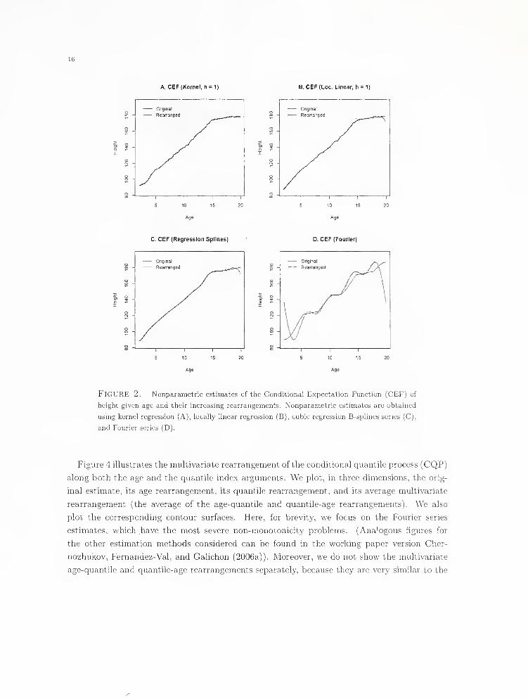
The panels A-D of Figure 2 show the original and rearranged estimates of the conditional

expectation function for the different methods. All the estimated curves have trouble capturing

the slowdown in the growth of height after age fifteen and yield non-monotonic curves for the

highest values of age. The Fourier series performs particularly poorly in approximating the

aperiodic age-height relationship and has many non-monotonicities. The rearranged estimates

correct the non-monotonicity of the original estimates, providing weakly increasing curves

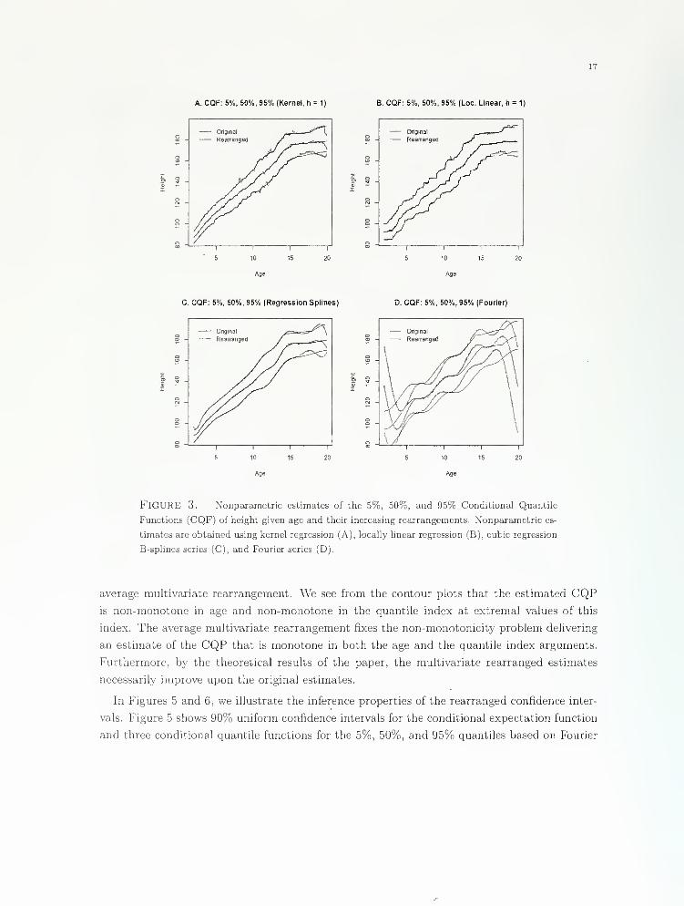
that coincide with the original estimates in the parts where the latter are monotonic. Figure

3 displays similar but more pronounced non-monotonicity patterns for the estimates of the

conditional quantile functions. In all cases, the rearrangement again performs well in delivering

curves that improve upon the original estimates and that satisfy the natural monotonicity

requirement. We quantify this improvement, in the next subsection.

16

A. CEF (Kernel, h = 1) B. CEF(Loc. Linear, h = 1)

15 20

Age Age

C. CEF (Regression Splines) D CEF (Fourier)

Age

10 15

Figure 2. Nonparamctric estimates of the Conditional Expectation Function (CEF) of

heiglit given age and their increasing rearrangements. Nonparamctric estimates are obtained

using kerne! regression (A), locally linear regression (B), cubic regression B-splines series (C),

and Fourier series (D).

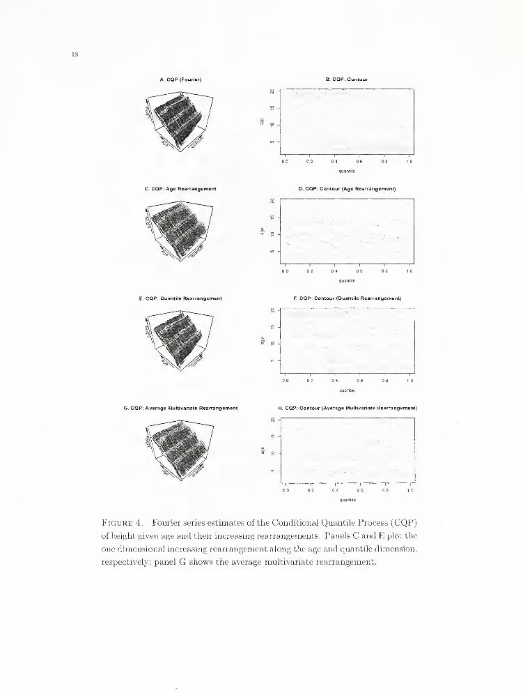
Figure 4 illustrates the multivariate rearrangement of the conditional quantile process (CQP)

along both the age and the quantile index arguments. We plot, in three dimensions, the orig-

inal estimate, its age rearrangement, its quantile rearrangement, and its average multivariate

rearrangement (the average of the age-quantile and quantile-age rearrangements). We also

plot the corresponding contour surfaces. Here, for brevity, we focus on the Fourier series

estimates, which have the most severe non-monotonicity problems. (Analogous figures for

the other estimation methods considered can be found in the working paper version Cher-

nozhukov, Fernandez-Val, and Galichon (2006a)). Moreover, we do not show the multivariate

age-quantile and quantile-age rearrangements separately, because they are very similar to the

17

A. CQF: 5%, 50%, 95% (Kernel, h = 1) B. CQF: 5%, 50%, 95% (Loc. Linear, h = 1)

Age

C. CQF: 5%, 50%, 95% (Regression Splines) D. CQF: 5%, 50%, 95% (Fourier)

Ags Age

Figure 3. Nonparamotric estimates of the 5%, 50%, and 95% Conditional Quantile

Functions (CQF) of height given age and their increasing rearrangements. Nonparametric es-

timates are obtained using Icernel regression (A), locally linear regression (B), cubic regression

B-splines series (C), and Fourier series (D). , ,,.

average multivariate rearrangement. We see from the contour plots that the estimated CQPis non-monotone in age and non-monotone in the quantile index at extremal values of this

index. The average multivariate rearrangement fixes the non-monotonicity problem delivering

an estimate of the CQP that is monotone in both the age and the quantile index arguments.

Furthermore, by the theoretical results of the paper, the multivariate rearranged estimates

necessarily improve upon the original estimates. . /

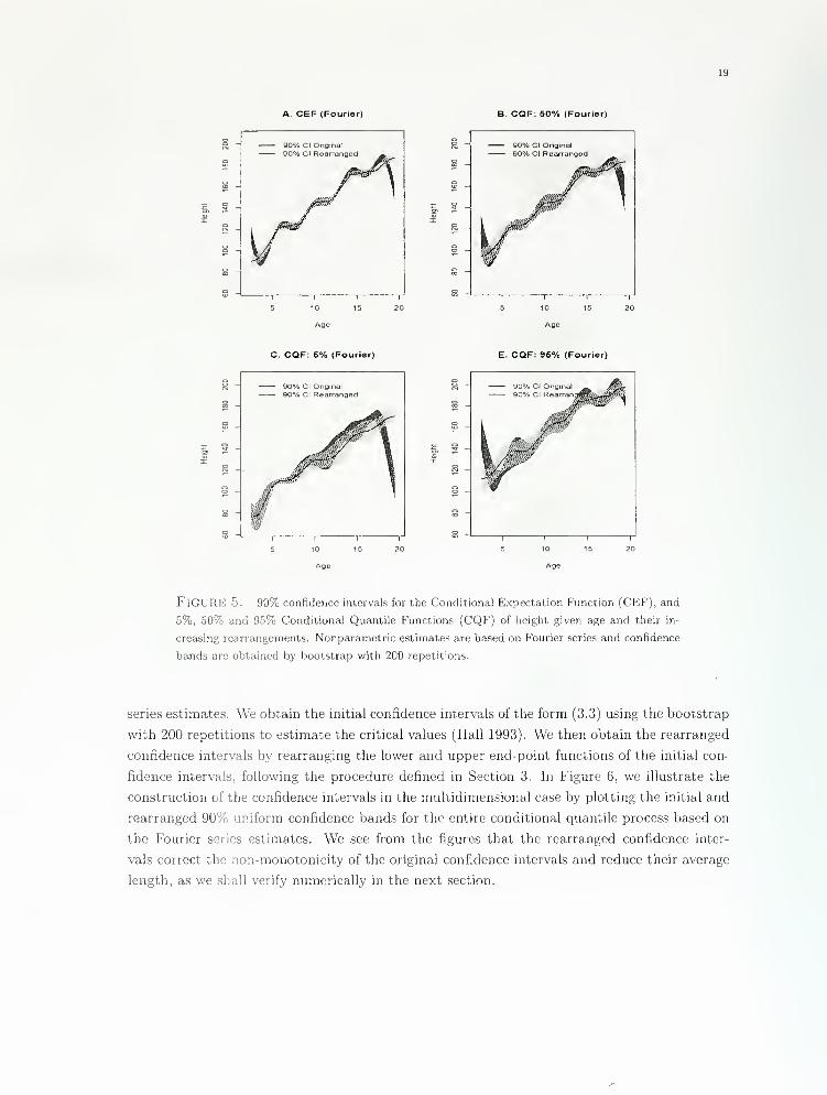
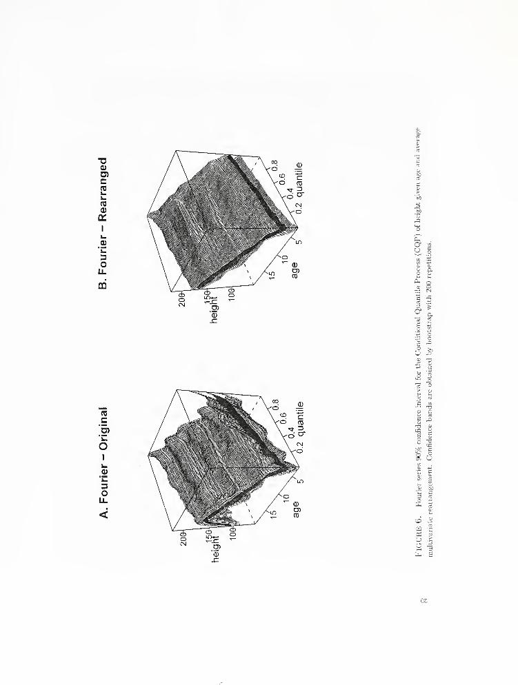
In Figures 5 and 6, we illustrate the inference properties of the rearranged confidence inter-

vals. Figure 5 shows 90% uniform confidence intervals for the conditional expectation function

and three conditional quantile functions for the 5%, 50%, and 95% quantiles ba,sed on Fourier

.18

A. CQP (Fourier) B. CQP: Contour

C. CQP: Age Rearrangement D. CQP; Contour (Age Rearrangement)

"T 1 1 1 1 T"

0.0 02 04 05 08 10

E. CQP: QuantJIe Rearrangement F. CQP: Contour (Quantile Rearrangement)

G. CQP: Average Multivariate Rearrangement H. CQP: Contour (Average Multivariate Rearrangement)

Figure 4. Fourier series estimates of the Conditional Quantile Process (CQP)

of height given age and their increasing rearrangements. Panels C and E plot the

one dimensional increasing rearrangement along the age and quantile dimension,

respectively; panel G shows the average multivariate rearrangement.

19

A. CEF (Fourier) B. CQF-. 60% (Fourier)

90% CI Onginal90Vo CI Rearrangod

90% CI Onginal90% CI Rearranged

C. CQF; 6% (Fourier) E. CQF: 96% (Fourier)

90% CI Original

90% CI Rearranged

Figure 5. 90% confidence intervals for the Conditional Expectation Function (CEF), and

5%, 50% and 95% Conditional Quantile Functions (CQF) of height given age and their in-

creasing rearrangements. Nonparamotric estimates are based on Fourier series and confidence

bands are obtained by bootstrap with 200 repetitions.

series estimates. We obtain the initial confidence intervals of the form (3.3) using the bootstrap

with 200 repetitions to estimate the critical values (Hall 1993). We then obtain the rearranged

confidence intervals by rearranging the lower and upper end-point functions of the initial con-

fidence intervals, following the procedure defined in Section 3. In Figure 6, we illustrate the

construction of the confidence intervals in the multidimensional case by plotting the initial and

rearranged 90% uniform confidence bands for the entire conditional quantile process based on

the Fourier series estimates. We see from the figures that the rearranged confidence inter-

vals correct the non-monotonicity of the original confidence intervals and reduce their average

length, as we shall verify numerically in the next section.'

,

Qi

G)C

m

OH

I

'^

O

d

T3

C3

> ,

"Eb;

j3

aQ.

"3 a!

c,o cyi

O

c J3o >iO JD

re

'5)

oI

.2

13

O

S J=

T3 OJ

tG CJ

GO 0^

o TjCG

g; C

§oa

tfl

_QJ

cCJ OJ

tfi

1- 0)0) bO^ c13 ao 1-,

eOjtH

CO 0)

ctiHQi SD >

O 3̂fe E

02

21

4.2. Monte-Carlo Illustration. The following Monte Carlo experiment quantifies the im-

provement in the point and interval estimation that rearrangement provides relative to the

original estimates. We also compare rearrangement to isotonization and to convex combina-

tions of rearrangement and isotonization.

Our experiment closely matches the empirical application presented above. Specifically, we

consider a design where the outcome variable Y equals a, location function plus a disturbance

e, Y = Z{Xyp + e, and the disturbance is independent of the regressor X . The vector Z{X)

includes a constant and a piecewise linear transformation of the regressor A' with three changes

of slope, namely Z(X) = (1,X,1{X > 5}{X -5),1{X > 10}-(A-10), 1{.Y > 15}- (A- 15)).

This design implies the conditional expectation function

E[Y\X] = Z{Xyp, (4,1)

and the conditional quantile function

QY{u\X) = Z{Xy/3+Q,{u). (4.2)

We select the parameters of the design to match the empirical example of growth charts in the

previous subsection. Thus, we set the parameter P equal to the ordinary least squares estimate

obtained in the growth chart data, namely (71.25, 8.13, ^2.72, 1.78, —6.43). This parameter

value and the location specification (4.2) imply a model for the CEF and CQP that is monotone

in age over the range of ages 2-20. To generate the values of the dependent variable, we draw

disturbances from a normal distribution with the mean and variance equal to the mean and

variance of the estimated residuals, e = Y — Z{X)'p, in the growth chart data. We fix the

regressor A' in all of the replications to be the observed values of age in the data set. In each

replication, we estimate the CEF and CQP using the nonparametric methods described in the

previous section, along with a global polynomial and a flexible Fourier methods. For the global

polynomial method, we fit a quartic polynomial. For the flexible Fourier method, we use a

quadratic polynomial and four trigonometric terms, with two sines and two cosines.

In Table 1 we report the average LP errors (for p = 1,2, and oo) for the original estimates

of the CEF. We also report the relative efficiency of the rearranged estimates, measured as

the ratio of the average error of the rearranged estimate to the average error of the original

estimate; together with relative efficiencies for an alternative approach based on isotonization

of the original estimates, and an approach consisting of averaging the rearranged and isotonized

estimates. The two-step approach based on isotonization corresponds to the SI estimator in

Mammen (1991), where the isotonization step is carried out using the pool-adjacent violator

algorithm (PAVA). For regression splines, we also consider the one-step monotone regression

splines of Ramsay (1998).

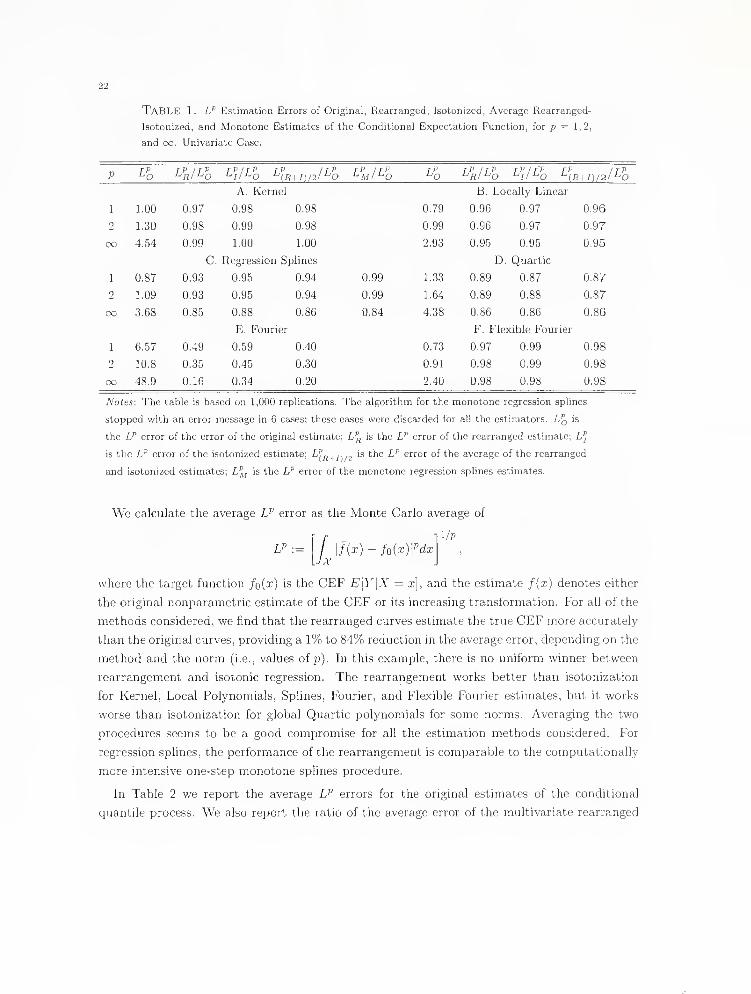
Table 1. L^ Estimation Errors of Original, Rearranged, Isotonizcd, Average Rearranged-

Isotonized, and Monotone Estimates of thie Conditional Expectation Function, for p = 1,2,

and oo. Univariate Case.

p L'o L'klL'o ^//^O ^\r+I)I2I^^0 L'm/L^o L'o L';,/L'^ L^JLl ^(fl+/)/2/-^0

A. Kernel B. Locally Linear

1 1.00 0.97 0.98 0.98 0.79 0.96 0.97 0.96

2 1.30 0.98 0.99 0.98 0.99 0.96 0.97 0.97

oo 4.54 0.99

C.

1.00 1.00

Regression Splines

2.93 0.95 0.95

D. Quartic

0.95

1 0.87 0.93 0.95 0.94 0.99 1.33 0.89 0.87 0.87

2 1.09 0.93 0.95 0.94 0.99 1.64 0.89 0.88 0.87

oo 3.68 0.85 0.88 0.86 0.84 4.38 0.86 0.86 0.86

E. Fourier F. Flexible Fourier

1 6.57 0.49 0.59 0.40 0.73 0.97 0.99 0.98

2 10.8 0.35 0.45 0.30 0.91 0.98 0.99 0.98

oo 48.9 0.16 0.34 0.20 2.40 0.98 0.98 0.98

Notes: The table is based on 1,000 replications. The algorithm for the monotone regression splines

stopped with an error message in 6 cases; these cases were discarded for all the estimators. Lq is

the L'' error of the error of the original estimate; L^ is the L'' error of the rearranged estimate; L;

is the L'' error of the isotonized estimate; i-f^./) ;2 '^ '^e L'' error of the average of the rearranged

and isotonized estimates; L^ is the L'' error of the monotone regression splines estimates.

We calculate the average L^ error as the Monte Carlo average of

i/p

LP \f(x)-Mx)\Pdx

where the target function fo{x) is the CEF E[Y'\X = x], and the estimate f{x) denotes either

the original nonparametric estimate of the CEF or its increasing transformation, For all of the

methods considered, we find that the rearranged curves estimate the true CEF more accurately

than the original curves, providing a 1% to 84% reduction in the average error, depending on the

method and the norm (i.e., values of p). In this example, there is no uniform winner between

rearrangement and isotonic regression. The rearrangement works better than isotonization

for Kernel, Local Polynomials, Splines, Fourier, and Flexible Fourier estimates, but it works

worse than isotonization for global Quartic polynomials for some norms. Averaging the two

procedures seems to be a good compromise for all the estimation methods considered. For

regression splines, the performance of the rearrangement is comparable to the computationally

more intensive one-step monotone splines procedure.

In Table 2 we report the average L^ errors for the original estimates of the conditional

quantile process. We also report the ratio of the average error of the multivariate rearranged

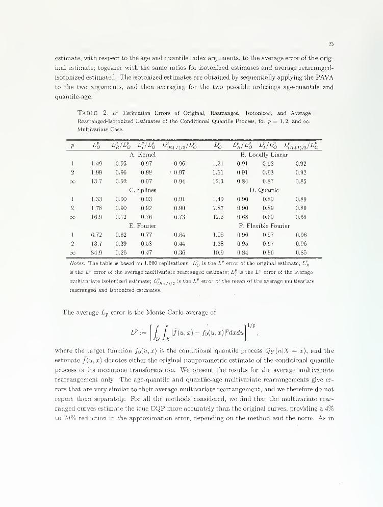
23

estimate, with respect to the age and quantile index arguments, to the average error of the orig-

inal estimate; together with the same ratios for isotonized estimates and average rearranged-

isotonized estimated. The isotonized estimates are obtained by sequentially applying the PAVA

to the two arguments, and then averaging for the two possible orderings age-quantile and

quantile- age.

Table 2. L'' Estimation Errors of Original, Rearranged, Isotonized, and Average

Rcarranged-Isotonized Estimates of the Conditional Quantile Process, for p = 1,2, and oo.

Multivariate Case.

p r'' tP irP^R/^O LVL'o

rP 1 TVi'o ^Rl^O LVL'o ^lR+I)/2l^O

A Kernel B. Locally Linear

1 1.49 0.95 0.97 0.96 1.21 0.91 0.93 0.92

2 1.99 0.96 0.98 0.97 1.61 0.91 0.93 0.92

oo 13.7 0.92

C.

0.97

Splines

0.94 12.3 0.84

D,

0.87

Quartic

0.85

1 1.33 0.90 0.93 0.91 1.49 0.90 0.89 0.89

2 1.78 0.90 0.92 0.90 1.87 0,90 0.89 0.89

00 16.9 0.72 0.76 0.73 12.6 0.68 0.69 0.68

E. Fourier F. Flexible Fou rier

1 6.72 0.62 0.77 0.64 1.05 0.96 0.97 0.96

2 13.7 0.39 0.58 0.44 1.38 0.95 0.97 0.96

oo 84.9 0.26 0.47 0.36 10.9 0.84 0.86 0,85

Notes: The table is based on 1,000 replications. Lq

is the L'' error of the average multivariate rearrange

is the L'' error of the original estimate; L^

d estimate; L^ is the L'' error of the average

multivariate isotonized estimate; LJ"^^, ,, is the L'' error of the mean of the average multivariate

rearranged and isotonized estimates.

The average Lp error is the Monte Carlo average of

LP:=/U JX

\f{u,x) - fo{u,x)\'''dxdu

i/p

where the target function fo(u,x) is the conditional quantile process Qy{u\X = x), and the

estimate f{u, x) denotes either the original nonparametric estimate of the conditional quantile

process or its monotone transformation. We present the results for the average multivariate

rearrangement only. The age-quantile and quantile-age multivariate rearrangements give er-

rors that are very similar to their average multivariate rearrangement, and we therefore do not

report them separately. For all the methods considered, we find that the multivariate rear-

ranged curves estimate the true CQP more accurately than the original curves, providing a 4%to 74% reduction in the approximation error, depending on the method and the norm. As in

24

the univariate case, there is no uniform winner between rearrangement and isotonic regression

and their average estimate gives a good balance.

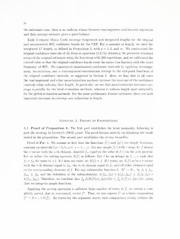
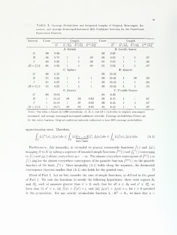
Table 3 reports Monte Carlo coverage frequencies and integrated lengths for the original

and monotonized 90% confidence bands for the CEF. For a measure of length, we used the

integrated L^ length, as defined in Proposition 3, with p = 1,2, and oo. We constructed the

original confidence intervals of the form in equations (3.3) by obtaining the pointwise standard

errors of the original estimates using the bootstrap with 200 repetitions, and we calibrated the

critical value so that the original confidence bands cover the entire true function with the exact

frequency of 90%. We constructed monotonized confidence intervals by applying rearrange-

ment, isotonization, and a rearrangement-isotonization average to the end-point functions of

the original confidence intervals, as suggested in Section 3. Here, we find that in all cases

the rearrangement and other monotonization methods increase the coverage of the confidence

intervals while reducing their length. In particular, we see that monotonization increases cov-

erage especially for the local estimation methods, whereas it reduces length most noticeably

for the global estimation methods. For the most problematic Fourier estimates, there are both

important increases in coverage and reductions in length.

Appendix A. Proofs of Propositions

A.l. Proof of Proposition 1. The first part establishes the weak inequality, following in

part the strategy in Lorentz's (1953) proof. The proof focuses directly on obtaining the result

stated in the proposition. The second part establishes the strong inequality.

Proof of Part 1. We assume at first that the functions /(•) and /o() are simple functions,

constant on intervals ((s - l)/r,s/r], s = 1, ...,r. For any simple /(•) with r steps, let / denote

the r-vector with the s-th element, denoted /s, equal to the value of /(•) on the s-th interval.

Let us define the sorting operator S{f) as follows: Let i be an integer in l,...,r such that

fe > Im for some m> I. If £ does not exist, set S{J) = f. U £ exists, set S{f) to be a r-vector

with the £-th element equal to fm, the m-th element equal to fg, and all other elements equal

to the corresponding elements of /. For any submodular function L : K^ —* K-|., by fi > fm,

fom > foe and the definition of the submodularity, L{fm,foe) + L{fc, forn) < L{hJw) +

L{fm,fom)- Therefore, we conclude that /_^, L(5(/)(x), /o(x))(ix <J,^ L{f{x), fo{3:))d2\ using

that we integrate simple functions.

Applying the sorting operation a sufficient finite number of times to /, we obtain a com-

pletely sorted, that is, rearranged, vector /*. Thus, we can express /* as a finite composition

/* = S o ... o S[f) . By repeating the argument above, each composition weakly reduces the

25

Table 3. Coverage Probabilities and Integrated Lengths of Original, Rearranged, Iso-

tonized, and Average Rcarrangcd-Isotonized 90% Confidenec Intervals for the Conditional

Expectation Function.

Interval Cover Length Cover Lengl:h

L' L'/L'o L'/Lh L^/L^ L' L '/Lh L-'/Ll L^/L^A. Kernel B. Locally Linear

.90 8.80 .90 8.63

R .96 8.79 1 1 .99 .96 8.63 1 1 .97

I .94 8.80 1 1 .99 .94 8.63 1 1 .98

(R + I)/2 .95 8.80 1

C. Splines

1 .99 .95 8.63

D,

1

Quartic

1 .97

.90 6.32 .90 10.43

R .91 6.32 1 1 1 .90 10.41 1 .99 .93

I .91 6.32 1 1 1 .90 10.43 1 1 .93

{R + I)/2 .91 6.32 1 1 1 .90 10.42 1 1 .93

E. Fourier F. Flexible Fourier

O .90 24.91 .90 6.45

R 1 24.52 .98 .94 0,63 .90 6.45 1 1 .97

I 1 24.91 1 .97 0.69 .90 6.45 1 1 .97

{R + I)/2 1 24.71 .99 .95 0.65 .90 6.45 1 1 .97

Notes: The table is based on 1,000 replications. O, R, /, and (R + /)/2 refer to original, rearranged,

isotonized, and average rearrangod-isotonizcd confidoncc intervals. Coverage probabilities (Cover) are

for the entire function. Original confidence intervals calibrated to have 90% coverage probabilities.

approximation error. Therefore,

/ L{r{x),fo{x))dx < f LiS^.^{f),fQ{x))dx < f L{f{x)Jo{x))dx. (A.l)Jx Jx T~r^- J'^'

nnitc times

Furthermore, this inequahty is extended to general measurable functions /() and /o(-)

mapping rV to /i' by taking asequence of bounded simple functions /''^'() and /q (•) converging

to /(•) and /o(-y almost everywhere as r -^ oo. The almost everywhere convergence of /'^^(O to

/() implies the almost everywhere convergence of its quantile function /*^'"^(-) to the quantile

function of the limit, /*()• Since inequality (A.l) holds along the sequence, the dominated

convergence theorem implies that (A.l) also holds for the general case. D

Proof of Part 2. Let us first consider the case of simple functions, as defined in the proof

of Part 1. We take the functions to satisfy the following hypotheses: there exist regions Xq

and Xq, each of measure greater than 5 > 0, such that for all x E Xq and x' G ^q, we

have that (i) x' > x, (ii) f{x) > f{x') + e, and (iii) fo{x') > fo{x) + e, for e > specified

in the proposition. For any strictly submodular function L : M? ~* M4. we have that rj =

26

ini{L{v',t) + L{v,t') — L{v,t) — L(v',t')} > 0, where the infimum is taken over all v,v' , t, t' in

the set K such that v' > v + c and t' > t + e. A simple graphical illustration for this property

is given in Figure 1.

We can begin sorting by exchanging an element f(x), x € Xq, of r-vector / with an element

f{x'), x' G Xq, of r-vector /. This induces a sorting gain of at least rj times 1/r. The total mass

of points that can be sorted in this way is at least 5. We then proceed to sort all of these points in

this way, and then continue with the sorting of other points. After the sorting is completed, the

total gain from sorting is at least 5r}. That is, /^ L{f*{x), fQ{x))dx < j-^ L{f{x),fo{x))dx — 5r].

We then extend this inequality to the general measurable functions exactly as in the proof

of part one. D

A. 2. Proof of Proposition 2. The proof consists of the following four parts.

Proof of Part 1. We prove the claim by induction. The claim is true for d = 1 by f*{x)

being a quantile function. We then consider any d > 2. Suppose the claim is true in d — 1

dimensions. If so, then the estimate f{xj,x-j), obtained from the original estimate f(x) after

applying the rearrangement to all arguments x_j of x, except for the argument x^, must be

weakly increasing in x_j for each Xj. Thus, for any x'_. > X-j, we have that

f{X„x'_^)>f(Xj,x^,)iorXj^U\0,l]. (A.2)

Therefore, the random variable on the left of (A.2) dominates the random variable on the right

of (A.2) in the stochastic sense. Therefore, the quantile function of the random variable on

the left dominates the quantile function of the random variable on the right, namely

f*{xj,x'_j) > f*{xj,x^j) for each Xj £ X = [0, 1]. (A. 3)

Moreover, for each x_j, the function Xj i—> f*{Xj,X-j) is weakly increasing by virtue of being

a quantile function. We conclude therefore that x i-^ f]{x) is weakly increasing in all of

its arguments at all points x € X"^. The claim of Part 1 of the Proposition now follows by

induction. - D

Proof of Part 2 (a). By Proposition 1, we have that for each x_j,

/\fj{xj,x~j) ~ fo{xj,x.j)\'' dxj <

/|/(xj,a;_j) - /o(Xj,x_j)|^dXj. (A. 4)

Now, the claim follows by integrating with respect to x_j and taking the p-th root of both

sides. For p = oo, the claim follows by taking the limit as p ^ oo. D

Proof of Part 2 (b). We first apply the inequality of Part 2(a) to J{x) = f{x), then to f{x) —

^d ° fi^)^ then to f{x) = R-k^.i ° Rtt^ ° /(^)i ^^'^ so on. In doing so, we recursively generate

a sequence of weak inequalities that imply the inequahty (2.6) stated in the Proposition. D

27

Proof of Part 3 (a). For each x-j £ A!'^~^ \ X-j, by Part 2(a), we have the weak inequality

(A. 4), and for each x-j S X-j, by the inequahty for the univariate case stated in Proposition

1 Part 2, we have the strong inequahty

XIfji^j^^ k{xj -])? dxj < / l/(ij,a;-j) - fQ{xj,x^j)\'' dxj - rjpS,

JX(A.5)

where T}p is defined in the same way as in Proposition 1. Integrating the weak inequality (A. 4)

over X-j & A'''"^ \ X-j, of measure I — i^, and the strong inequahty (A.5) over X^j, of measure

v, we obtain

.vf;{x)-fo{x)\''dx< / \f{x)-fQ{x)fdx-^M.

Xd(A.6)

The claim now follows. D

Proof of Part 3 (b). As in Part 2(a), we can recursively obtain a sequence of weak inequalities

describing the improvements in approximation error from rearranging sequentially with respect

to the individual arguments. Moreover, at least one of the inequahties can be strengthened

to be of the form stated in (A.6), from the assumption of the claim. The resulting system of

inequalities yields the inequality (2.8), stated in the proposition.

Proof of Part 4. We can write

x"

D

r(^-)-- /o(x) 'dx1/p

Jx''

1

,,, ): ^-hin L

^E (/"(-) -/o(-)TrGn

X-if;{x) - Mx)

dx

!/p

1/p

(A.7)

dx

where the last inequality follows by pulling out l/|n| and then applying the triangle inequality

for the L-p norm. D

A. 3. Proof of Proposition 3. Proof of Part 1. The monotonicity follows from Proposition 2.

The rest of the proof relies on establishing the order-preserving property of the 7r-rearrangement

operator: for any measurable functions p, m : X'^ have that

g{x) < m{x) for all x £ X implies g*{x) < m*{x) for all x G X" (A.8)

Given the property we have that

e(x) < f{x) < u(x) for all x e X'^ implies t(x) < f*{x) < u*(x) for all x e X'^

,

which verifies the claim of the first part. The claim also extends to the average multivariate

rearrangement, since averaging preserves the order-preserving property.

It remains to establish the order-preserving property for tt— rearrangement, which we do

by induction. We first note that in the univariate case, when d = 1, order preservation is

obvious from the rearrangement being a quantile function; the random variable m{X), where

28

X ~ Uniform[A'], dominates the random variable g{X) in the stochastic sense, hence the

quantile function m*{x) of m{X) must be greater than the quantile function g*{x) of g{X)

for each x £ X . We then extend this to the multivariate case by induction: Suppose the

order-preserving property is true for any d — I with d > 2. If so, then for each Xj G A^ and

g{xj,X--j) < m[xj,x-j) implies g{xj,x-j) < fh{xj,X-j),

where g and in are multivariate rearrangements of X-j i-^ g{xj,x-j) and x_j ^^ m{xj,x-j)

with respect to x-j , holding Xj fixed. Now apply the order-preserving property of the univariate

rearrangement to the univariate functions Xj i-^ g{xj,X-j) and Xj ^-> fh{xj,X-j), holding x-j

fixed, for each X-j, to conclude that (A. 8) holds. D

Proof of Part 2. As stated in the text, the weak inequality is due to Lorentz (1953).

For completeness we only briefly note that the proof is similar to the proof of Proposition

1. Indeed, we can start with simple functions £() and u(-) and work with their equiv-

alent vector representations i and u. Then we apply the two point sort operation S to

both i and u. By the definition of submodularity (2.3), each application of S weakly re-

duces submodular discrepancies between vectors, so that pairs of vectors in the sequence

{(£, u), {S{i), S{u)), ..., {So...oS{C), So...oS{u)), (i*,u*)} become progressively weakly closer to

each other, and the sequence can be taken to be finite, where the last pair is the rearrangement

{i*,u*) of vectors {£,u). The inequality extends to general bounded measurable functions by

passing to the limit and using the dominated convergence theorem. To extend the proof to the

multivariate case, we apply exactly the same induction strategy as in the proof of Proposition

2. D

Proof of Part 3. Finally, the proof of strict inequality in the univariate case is similar to

the proof of Proposition 2, using the fact that for strictly submodular functions L : K^ t-^ R+

we have that t] = in{{L{v',t) + L{v,t') — L{v,t) — L{v',f')} > 0, where the infimum is taken

over all v, v', t, t' in the set K such that v' > v + e and t' > t + e or such that v > v' + e and

t > t' + £. The extension of the strict inequality to the multivariate case follows exactly as in

the proof of Proposition 2. . D

References

Andrews, D. W. K. (1991): "Asymptotic normality of series estimators for nonparametric and semiparametric

regression models," Econometnca, 59(2), 307-345.

Ayer, M., H. D. Brunk, G. M. EwiNG, W. T. Reid, and E, Silverman (1955): "An empirical distribution

function for sampling with incomplete information," Ann. Math. Statist., 26, 641-647.

Barlow, R. E.. D. J. Bartholomew, J. M. Bremner, and H. D. Brunk (1972): Statistical inference

under order restrictions. The theory and application of isotonic regression. John Wiley & Sons, London-New

York-Sydney, Wiley Series in Probability and Mathematical Statistics.

29

ChaUDHURI, p. (1991): "Nonparamctric estimates of regression quantilcs and their local Bahadur representa-

tion," Ann. Statist., 19, 760-777.

Chernozhukov, v., I. Fernandez-Val, and A. Galichon (2006a): "Innproving Approximations of Mono-

tone Functions by Rearrangement," MIT and UCL CEMMAP Working Paper, available at www.arxiv.org,

cemmap.ifs.org.uk, www.ssrn.com.

(2006b): "Quantile and Probability Curves without Crossing," MIT and UCL CEMMAP Working

Paper, available at www.arxiv.org, cemmap.ifs.org.uk, www.ssrn.cbm.

(2006c): "Rearranging Edgeworth-Cornish-Fisher Expansions," MIT and UCL CEMMAP Working

Paper, available at www.arxiv.org, cemmap.ifs.org.uk, www.ssrn.com.

Cole, T. J. (1988): "Fitting smoothed centile curves to reference data," J Royal Stat Soc, 151, 385-418.

DavydOV, Y., and R. ZlTIKIS (2005): "An index of monotonicity and its estimation: a step beyond econometric

applications of the Gini index," Metron, 63(3), 351-372.

Dette. H., N. Neumeyer, and K. F. Pilz (2006): "A simple nonparamctric estimator of a strictly monotone

regression function," Bernoulli, 12(3), 469-490.

Dette. H., and K. F. Pilz (2006): "A comparative study of monotone nonparametric kernel estimates," J.

Stat. Comput. Sxmul., 76(1), 41-56.

Dette, H., and R. Scheder (2006): "Strictly monotone and smooth nonparametric regression for two or

more variables," The Canadian Journal of Statistics, 34(4), 535-561.

Fan, J., and I. GubelS (1996): Local polynomial modelling and its applications, vol. 66 of Monographs on

Statistics and Applied Probability. Chapman h Hall, London.

Fougeres, A.-L. (1997): "Estimation de densites unimodales," The Canadian .Journal of Statistics / La Revue

Canadienne de Statistique, 25(3), 375-387.

Gallant, A. R. (1981): "On the bias in flexible functional forms and an essentially unbiased form: the Fourier

flexible form," J. Econometrics, 15(2), 211-245.

GenoveSE. C, and L. Wasserman (2008): "Adaptive confidence bands," Ann. Statist., 36(2), 875-905.

Hall, P. (1993): "On Edgeworth Expansion and Bootstrap Confidence Bands in Nonparametric Curve Esti-

mation," Journal of the Royal Statistical Society. Series B (Methodological), 55(1), 291-304.

Hardy, G. H., J. E. Littlewood, and G. Polya (1952): Inequalities. Cambridge University Press, 2d ed.

He. X., AND Q.-M. Shao (2000): "On parameters of increasing dimensions," J. Multivariate Anal., 73(1),

120-135.

JOHANSEN, S., AND I. M. JOHNSTONE (1990): "HotcUing's theorem on the volume of tubes: some illustrations

in simultaneous inference and data analysis," Ann. Statist., 18(2), 652-684.

Knight, K. (2002): "What are the limiting distributions of quantile estimators?," in Statistical data analysis

based on the Li-norm and related methods (Neuchdtel, 2002), Stat. Ind. Techno!., pp. 47-65. Birkhauser, Basel.

KOENKER, R- (2008): quantreg: Quantile RegressionK package version 4.17.

KOENKER, R,, AND G. S. Bassett (1978): "Regression quantiles," Econometnca, 46, 33-50.

KOENKER, R., AND P. Ng (2005): "Inequality constrained quantile regression," Sankhyd, 67(2), 418-440.

Lehmann, E. L., AND J. P. Romano (2005): Testing statistical hypotheses, Springer Texts in Statistics.

Springer, New York, third edn.

Lorentz, G. G. (1953): "An inequality for rearrangements," Timer. Math. A4onthly, 60, 176-179.

Mammen, E. (1991): "Nonparamctric Regression Under Qualitative Smoothness Assumptions," The Annals of

Statistics, 19(2), 741-759.

Mammen, E., J. S. Marrow. B. A. Turlach, A'ND M. P. Wand (2001): "A general projection framework

for constrained smoothing," Statist. Sci., 16(3), 232-248. -

30

Matzkin, R. L. (1994): "Restrictions of economic theory in nonparametric methods," in Handbook of econo-

metrics, Vol. IV, vol. 2 of Handbooks in Econom., pp. 2523-2558. North-Holland, Amsterdam.

Newey, W. K. (1997): "Convergence rates and asymptotic normality for series estimators," J. Econometrics,

79(1), 147-168.

PORTNOY, S. (1997): "Local asymptotics for quantilc smoothing splines," Ann. Statist., 25(1), 414-434.

R Development Core Team (2008): R: A Language and Environm.ent for Statistical Com.putingR Foundation

for Statistical Computing, Vienna, Austria, ISBN 3-900051-07-0.

Ramsay, J. O. (1988): "Monotone Regression Splines m Action," Statistical Science, 3(4), 425-441.

Ramsay. J. 0., and B. W. Silverman (2005): Functional data analysis. Springer, New York, second edn.

Ramsay, J. O., H. Wickham, and S. Graves (2007): fda: Functional Data AnalysisR package version 1,2.3.

Robertson, T., F. T. Wright, and R. L. Dykstra (1988): Order restricted statistical inference, Wiley

Series in Probability and Mathematical Statistics: Probability and Mathematical Statistics. John Wiley &Sons Ltd., Chichester.

SiLVAPULLE, M. J., AND P. K. SEN (2005): Constrained statistical inference, Wiley Series in Probability and

Statistics. Wiley-Interseience [.3ohn Wiley & Sons), Hoboken, NJ.

Stone, C. J. (1994): "The use of polynomial splines and their tensor products in multivariate function estima-

tion," Ann. Statist., 22(1), 118-184, With discussion by Andreeis Buja and Trevor Hastie and a rejoinder by

the author.

VlLLANl, C. (2003): Topics in optimal transportation, vol. 58 of Graduate Studies m Mathematics. American

Mathematical Society, Providence, RI.

Wand, M. P., and M. C. Jones (1995): Kernel smoothing, vol, 60 of Monographs on Statistics and Applied

Probability. Chapman and Hall Ltd., London.

Wasserman, L. (2006): All of nonparametric statistics. Springer Texts in Statistics. Springer, New York.

Wei, Y., A. Pere, R. Koenker, and X. He (2006): "Quantile regression methods for reference growth

charts," Stat. Med., 25(8), 1369-1382.