Improvement of the MSR1a algorithm in the WIEN2kcode

Theo Guerber

Acknowledgement

First, I would like to acknowledge Xavier Rocquefelte for offering me a veryrewarding internship and for being my tutor during this one.

I would like to express my very great appreciation Laurence Marks for workingwith me throughout the internship.

I acknowledge Yvon Lafranche for agreeing to be my reference teacher.

I thank the CTI team of ISCR for hosting me during my internship.

1

Abstract

Researchers working in theoretical chemistry work not with chemical com-pounds and glassware but with molecular and solid optimization software. Theseprograms are based on optimization algorithms. The topic for my internshipwas to try to improve the algorithm named MSR1 of WIEN2K software usedfor density functional theory. The problem is that due to calculations of eigen-values and of eigenvectors of matrices of considerable size, an iteration of thealgorithm can take from a few minutes to several hours. Thus, the ideal is forthe algorithm to converge but in a reduced number of iterations.So I first did a bibliography and studied the associated mathematical theorythat I present in chapter 1. Then, I coded a program in MATLAB language inorder to obtain usable data that I present in chapter 2. Finally, I analyzed thedata collected in order to find useful clues for the improvement of the algorithm,results that allowed an advance and a future upgrade of the software, all this ispresented in chapter 3.

2

Table of Contents

Acknowledgment 3

Abstract 3

1 Internship’s context 41.1 ISCR presentation . . . . . . . . . . . . . . . . . . . . . . . . . . 4

1.1.1 CTI (Chimie Theorique Inorganique) team . . . . . . . . 41.1.2 WIEN2K problematic . . . . . . . . . . . . . . . . . . . . 4

1.2 Density functional Theory . . . . . . . . . . . . . . . . . . . . . . 51.2.1 Kohn-Sham equations . . . . . . . . . . . . . . . . . . . . 51.2.2 Fixed-point theory . . . . . . . . . . . . . . . . . . . . . . 5

1.3 State of the art . . . . . . . . . . . . . . . . . . . . . . . . . . . . 61.3.1 Quasi-Newton method . . . . . . . . . . . . . . . . . . . . 61.3.2 Approximation of matrix Hn in MSR1 algorithm . . . . . 6

2 Modelling and programming 82.1 Modelling of a "WIEN2K mixer" . . . . . . . . . . . . . . . . . . 8

2.1.1 Choice of programming language . . . . . . . . . . . . . . 82.1.2 Recreation of MSR1 algorithm . . . . . . . . . . . . . . . 82.1.3 Test functions . . . . . . . . . . . . . . . . . . . . . . . . . 11

2.2 Transformation in a "real" program . . . . . . . . . . . . . . . . 122.2.1 IHM . . . . . . . . . . . . . . . . . . . . . . . . . . . . . . 122.2.2 Functions . . . . . . . . . . . . . . . . . . . . . . . . . . . 142.2.3 Algorithm . . . . . . . . . . . . . . . . . . . . . . . . . . . 14

3 Result and futurs researchs 153.1 Tests and results . . . . . . . . . . . . . . . . . . . . . . . . . . . 15

3.1.1 Iteration according to α . . . . . . . . . . . . . . . . . . . 153.1.2 Eigenvalues/Eigenvectors of Hn . . . . . . . . . . . . . . . 163.1.3 Study of eigenvalues/eigenvectors of the other matrices of

the algorithm . . . . . . . . . . . . . . . . . . . . . . . . . 173.2 Conclusion of the results and future prospects . . . . . . . . . . . 17

3.2.1 Contribution of the internship . . . . . . . . . . . . . . . . 173.2.2 Trust-region control . . . . . . . . . . . . . . . . . . . . . 18

3

Chapter 1

Internship’s context

1.1 ISCR presentationThe Beaulieu campus brings together a large number of infrastructures dedi-

cated to research. I did my internship in the one dedicated to chemistry: Institutdes sciences chimiques de Rennes (ISCR). ISCR has 280 permanent staff andseveral research teams. I worked with the CTI (Chimie Theorique Inorganique)team.

1.1.1 CTI (Chimie Theorique Inorganique) teamThe CTI team works differently from other teams. Where the majority of

other teams use chemistry equipment, the CTI team uses server clusters. Thisteam uses many softwares often designed by the chemists themselves. Thesesoftwares often have the function of solving chemical equations as for examplethe Schrodinger equation. Most of the time, software calculations are staggering,hence the use of server clusters. The idea behind my involvement with the CTIteam was to try to improve the computational time of the software. The softwareto which I have contributed is called WIEN2K.

1.1.2 WIEN2K problematicLaurence Marks, the researcher I worked with during my internship, has al-

ready made improvements to WIEN2K and has written an article about it. Thisarticle was the core of my internship.WIEN2K is linked to two complementaryalgorithms. Laurence Marks’ idea is to perform a linear combination of thesetwo algorithms. So I worked during my internship on this linear combinationin order to extract information that could make it optimal. But before I startexplaining what I did during my internship, I will first explain the chemicaltheory related to WIEN2K and the state of the art of the WIEN2K algorithm.

4

1.2 Density functional TheoryAs stated on the website dedicated to the WIEN2k software: WIEN2k allows

to perform electronic structure calculations of solids using density functionaltheory (DFT). I will not detail all the DFT here but focus on what concernsme mainly in the DFT, the Kohn-Sham equations.

1.2.1 Kohn-Sham equationsKohn-Sham equations are equations of the type Schrodinger equations, that

is equations whose solutions are eigenfunctions and eigenvalues.

HKSΦk = εkΦk (1.1)

Here, HKS is a functional, Φk eigenfunctions and εk eigenvalues. Due to thenature of the functional, these equations can only be resolved in an iterativeapproach. Moreover, since chemists are required to solve this equation in thecase of solids, the resolution of an iteration can take a long time, this adds aconstraint, the algorithm to be optimized must converge but must also convergein few iterations. Mathematically, this can therefore be summed up as a fixedpoint problem on a vector function.

1.2.2 Fixed-point theoryLet us consider a vector function F, that is to say:

F : RN → RN (1.2)

Finding a fixed point of F is like finding x∗ ∈ RN such that :

F (x∗) = x∗ (1.3)

Let’s put G, an other vector function, as:

G : x→ F (x)− x (1.4)

Finding a fixed point of F is like finding a root of G. One method to findan approximate value of x∗ is Newton’s generalized method at these vectorfunctions. x∗ becomes the limit of a series (xn) whose recurrence is:

xn+1 = xn − JG(xn)−1.G(xn) (1.5)

where JG is the jacobian matrix of the function G. That is:

JG(xn) = Bn B−1n = Hn ∈MN (R) bi,j =∂gi∂xj

(1.6)

In the context of the DFT, the number of unknown, N, of the vector functioncould reach values in the order of 104. In this case, calculating the inverse of amatrix of this size becomes prohibitive at the level of computational costs. Anapproximation of the matrix is therefore necessary.

5

1.3 State of the artThe approximation of the matrix and which method to choose to approxi-

mate hold a central place in the article by Laurence Marks. Indeed, the linearcombination I mentioned earlier is a linear combination of two approximationsof this Hn matrix. In the event that the calculation of H is too expensive, theNewton method is therefore applied with a matrix approximated according tothe previous ones. Newton’s method then becomes a quasi-newton method.

1.3.1 Quasi-Newton methodIn a Quasi-Newton’s method, we don’t calculate the matrix Hn, we approxi-

mate it. The idea is a generalization of the secant method for multidimensionalproblems.

B̃n.(xn − xn−1) = G(xn)−G(xn−1) (1.7)

where B̃n is the approximation of the Jacobian. There are several methods toapproximate this matrix. The best known methods are:

• Davidon-Fletcher-Powell (DFP)

• Broyden-FLetcher-Goldfarb-Shanno (BFGS)

• Symmetric rank one

• "Good" and "Bad" Broyden

It has been shown in previous work[1] that it is the Broyden methods that aremost suitable in the context of DFT.

1.3.2 Approximation of matrix Hn in MSR1 algorithmAs mentioned earlier, the algorithm in WIEN2K is a linear combination of

the two Broyden algorithms. This algorithm being the core of my internship, wewill detail its functioning in order to fully understand the associated problem.

"Good" and "Bad" Broyden

First of all, we introduce new variables :

yj,n = G(xn)−G(xj) (1.8)sj,n = xn − xj (1.9)

In his article, Broyden used two methods[2]. The first, referred to "good" Broy-den’s method is to find an approximation of Bn in respect of Frobenius norm.So we have[1] :

Bn+1 = Bn +(yn − σnBnsn)sTn

σn||sn||2(1.10)

6

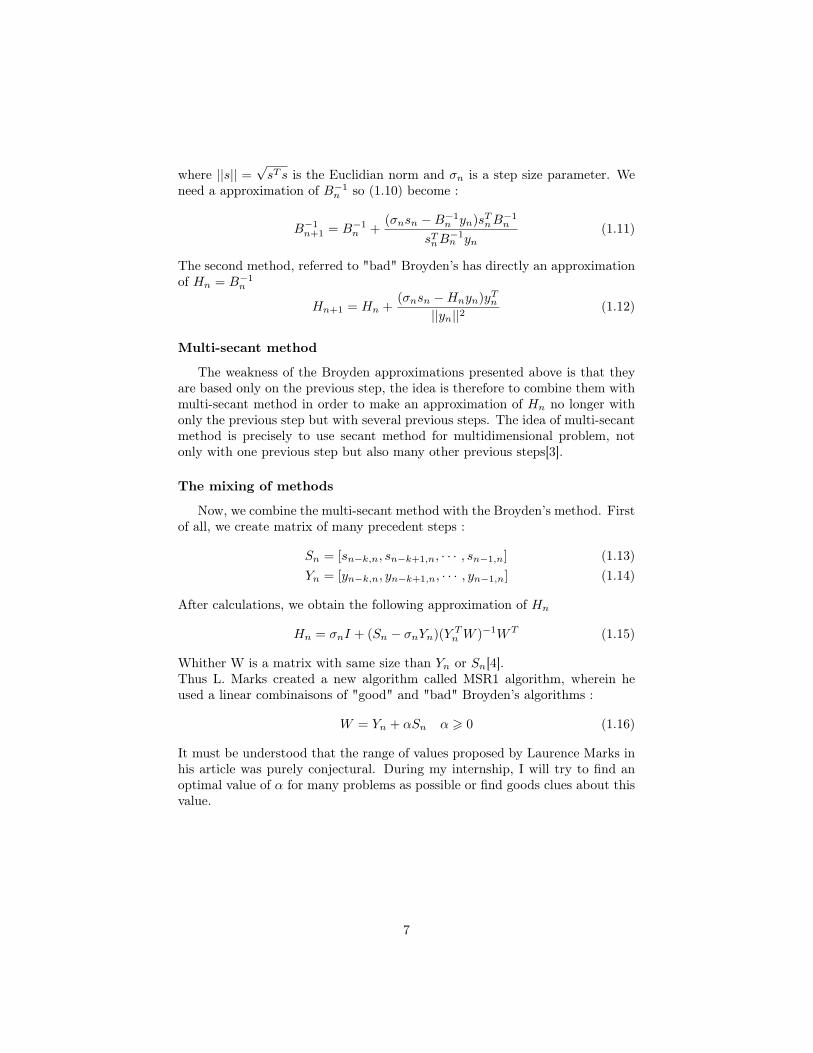
where ||s|| =√sT s is the Euclidian norm and σn is a step size parameter. We

need a approximation of B−1n so (1.10) become :

B−1n+1 = B−1n +(σnsn −B−1n yn)sTnB

−1n

sTnB−1n yn

(1.11)

The second method, referred to "bad" Broyden’s has directly an approximationof Hn = B−1n

Hn+1 = Hn +(σnsn −Hnyn)yTn

||yn||2(1.12)

Multi-secant method

The weakness of the Broyden approximations presented above is that theyare based only on the previous step, the idea is therefore to combine them withmulti-secant method in order to make an approximation of Hn no longer withonly the previous step but with several previous steps. The idea of multi-secantmethod is precisely to use secant method for multidimensional problem, notonly with one previous step but also many other previous steps[3].

The mixing of methods

Now, we combine the multi-secant method with the Broyden’s method. Firstof all, we create matrix of many precedent steps :

Sn = [sn−k,n, sn−k+1,n, · · · , sn−1,n] (1.13)Yn = [yn−k,n, yn−k+1,n, · · · , yn−1,n] (1.14)

After calculations, we obtain the following approximation of Hn

Hn = σnI + (Sn − σnYn)(Y Tn W )−1WT (1.15)

Whither W is a matrix with same size than Yn or Sn[4].Thus L. Marks created a new algorithm called MSR1 algorithm, wherein heused a linear combinaisons of "good" and "bad" Broyden’s algorithms :

W = Yn + αSn α > 0 (1.16)

It must be understood that the range of values proposed by Laurence Marks inhis article was purely conjectural. During my internship, I will try to find anoptimal value of α for many problems as possible or find goods clues about thisvalue.

7

Chapter 2

Modelling and programming

2.1 Modelling of a "WIEN2K mixer"I had the idea to create a fictitious model of the algorithm of L. Marks

because I wanted to observe the number of iterations according to the value ofα with test functions found in the literature.

2.1.1 Choice of programming languageThe choice of the programming language was made naturally, knowing in

advance that the algorithm would have to manipulate matrices of consequencesizes, I chose the language created with the aim of manipulating matrices: MAT-LAB.Its downside is that it is not opensource like other language but I had a licenseon my personal computer during the internship and if it had been necessary, itwas always possible to transpose the work into a free equivalent like Scilab.

2.1.2 Recreation of MSR1 algorithmHere I will present the algorithm I created based on the work of L. Marks.

In section 1.3.2, I presented the general idea of the MSR1 algorithm, here wewill explain the different parts of the algorithm (initialization, regularizationand pseudo-inversion) whose purpose is to find a root of the following function:

F : RN → RN (2.1)

Initialization

As I said in section 1.3.1, the algorithms of the quasi-Newton methods usethe results of the previous step or steps. But as we see on equations (1.8) and(1.9), as a difference is made, it is necessary to have at least two points.

8

The test functions I acquired were presented with an initial point x0. Inorder not to start in the wrong "direction", the point x1 is calculated as follows:

x1 = x0 − p · F (x0) (2.2)

Where p is a arbitrary value analogous to Pratt step[4]. In my program the pvalue was set to: 0.01.

Approximation of JF (xn)−1

We need to find a good value of Hn approximation of JF (xn)−1. In orderto best recreate the MSR1 algorithm, I drew on the algorithm presented in thetwo articles by L. Marks.[4][1].First of all, like in the section 1.3.2, I create new variables

yj,n = F (xn)− F (xj) (2.3)

sj,n = xn − xj (2.4)

and associated matrix :

Sn = [sn−k,n, sn−k+1,n, · · · , sn−1,n] (2.5)Yn = [yn−k,n, yn−k+1,n, · · · , yn−1,n] (2.6)

Then, I create a regularization matrix Ψn[1]. The use of the regularization ma-trix helps to avoid creating instability related to the accuracy of the calculations.In fact, the closer we get to the root the closer the matrix Yn gets to the nullmatrix, the regularization gets closer to a normalization of the matrix Yn.

Ψn =

1/||yn−k,n|| 0 · · · 0

0 1/||yn−k+1,n||. . .

......

. . . . . ....

0 · · · 0 1/||yn−1,n||

(2.7)

Finally, I create the following matrices, always based on the work of L. Marks[1]:

An = ΨnYTn (Yn + αSn)Ψn (2.8)

Hn = σnI + (Sn − σnYn)ΨnA−1n Ψn(Yn + αSn)T (2.9)

Here, σn is what L. Marks calls algorithm greed in his article[4]. The notion ofalgorithm greed is important because as L. Marks says in his article, a majordifference between the "Good" and "Bad" Broyden algorithm is the fact of beinga greedy algorithm or not. A definition of an greedy algorithm given in the articleof L. Marks is as follows:

A greedy algorithm always makes the choice that looks best at themoment. That is, it makes a locally optimal choice in the hope thatthis choice will lead to a globally optimal solution.

9

In order to focus on the linear combination of the two algorithms, it was chosento take a constant σn value.

σn = σ = 0.01 (2.10)

Singular value decomposition

As we see in equations (2.8) and (2.9), matrix An must be inverted but thatmatrix can be singular(not invertible). So we don’t calculate the inverse butthe pseudo-inverse. Suppose that we need to invert A. First of all, we used asingular-value decomposition.

A = USV T (2.11)

S is a singular matrix (diagonal matrix with singular values of A). On MATLAB,I use the command svd to find U,V,S. After that, we create the pseudo-inverseof S.

s+ij =sij

s2ij + β(2.12)

β is a constant added to the denominator to avoid divisions by zero. Finally,the pseudo-inverse of A, B is created :

B = V S+UT (2.13)

Thus, in my algorithm, the equation to calculate Hn is the following :

Hn = σnI + (Sn − σnYn)ΨnBnΨn(Yn + αSn)T (2.14)

with Bn the pseudo-inverse of An.

Divergence

In some cases, we have a divergence of the algorithm, ||F (xn)|| −→ +∞. So,if ||F (xn)|| exceeds a certain value, the algorithm is stopped and the number ofiteration is fixed to a arbitrary value.

||F (xn)|| > M Niter(α) = Nitermax ∗ 1.1 (2.15)

Stop criterion

In order not to have an algorithm stuck in an endless loop, I set a stopcriterion related to the number of iterations. thus, if the algorithm exceeds anumber of iterations set by the user, it stops even if the stop criterion linked tofunction F is not yet reached.

10

The function-related shutdown criterion is the one that when achieved firstshows the effectiveness of the algorithm. Since the goal of the algorithm is toreach an F root, we set an ε criterion such that we have:

||F (xn)|| < ε (2.16)

the algorithm stops.

2.1.3 Test functionsIn order to represent as accurately as possible the calculations occurring in

WIEN2K software, it was necessary to use test functions whose size was notfixed in advance and could be chosen by the user. It was also necessary thatthe functions found give with the algorithm created exploitable results.

After some research, here are the test functions used in the MATLAB pro-gram. They come from an article testing different algorithms using quasi-Newton methods[5]. In short, the role of the test functions is to simulate afixed point problem with a large vector function. Thus the functions shownbelow are vector functions of which we know the existence of a fixed point.They were also selected by the researchers to test the robustness and speed ofconvergence of algorithms using quasi-Newton methods.

The extended Rosenbrock function

F2i−1(x) = 10(x2i − x22i−1)

F2i(x) = 1− x2i−1i = 1, · · · , m

2(2.17)

The extended Powell function

F4i−3(x) = x4i−3 + 10x4i−2

F4i−2(x) =√

5(x4i−1 − x4i)F4i−2(x) = (x4i−2 − 2x4i−1)2

F4i(x) =√

10(x4i−3 − x4i)2

i = 1, · · · , m4

(2.18)

The Broyden tridiagonal function

Fi(x) = (3− 2xi)xi − xi−1 − 2xi+1 + 1

x0 = xm+1 = 0i = 1, · · · ,m (2.19)

11

The Broyden banded function

Fi(x) = xi(2 + 5x2i ) + 1−∑j∈Ji

xj(1 + xj)

Ji = {j : j 6= i,max(1, i−ml) 6 j 6 min(m, i+mu)}ml = 5,mu = 1

i = 1, · · · ,m (2.20)

The Brown almost-linear function

Fi(x) = xi +∑

j = 1mxj − (n+ 1) 1 6 i < m

Fm(x) =

m∏j=1

xj

− 1(2.21)

2.2 Transformation in a "real" programAlong with the work of running the algorithm and studying the resulting

data, I had the will to make it a real program with a minimum of human-machine interface in order to be able to manipulate the algorithm more easily.

Thus, at the end of the course, the program is presented in the form shownin figure 1 in the appendix.

The program consists of three parts:

• Human-machine interface (IHM in french)

• Functions

• Algorithm

2.2.1 IHMThis part of the program aims to simplify the launch of the program, because

although it is a very simplified version of a part of WIEN2K, it is neverthelessrather complex. The first dialog box, called "Function Selector" allows the userto choose which test function he will use (cf figure 2). The choice to put thefunction selection before selecting the values of the parameters internal to thealgorithm is that each function does not have the same values for which theresults are useful.For this reason, depending on the function chosen by the user,the default parameter values that can be chosen by the user are not the same.

As we see in figure 3, the parameters that can be modified are the parametersthat we discussed in the sections above.

12

α:

The choice of the first parameter is particular because it will not set a valuefor alpha but create a vector containing all the alpha values between the minvalue and the max value chosen with the chosen step between each value. Foreach alpha value, we will run the algorithm and retrieve data specific to thatvalue.

β:

The goal of β is to be able to create a pseudo-inverse as just as possible,this value represents the compromise between getting as close as possible to themathematical limit while avoiding calculation errors due to zero machine

σ:

As explained in section 2.1.2, the sigma parameter is algorithm greed. Al-though it has been set to 0.01 by default, the user can always change it if desired,however, the fact that it varies with each iteration has not been implementedin the program.

"Pratt step" :

As just above, the "Pratt step" is explained in the section 2.1.2. It can ofcourse also be changed by the user.

Number of variables :

This number refers to N in equation (2.1). In the context of DFT, the orderof magnitude of N is 104 but in order to limit memory requirements and shortencalculation times, the default value is 200. This value is high enough to allowthrough a sufficient number of data as will be seen later.

Iteration maximum :

This parameter allows the algorithm to stop if there is no convergence. Ihad to vary its value regularly during my tests during my internship. This willbe detailed in the next chapter but to sum up, by increasing it sufficiently, I wasable to reveal cases of very slow convergence (oscillation before convergence).

ε :

This parameter is the stop criterion of the algorithm. In order to ensurethat we have a convergence and not just an oscillation or a "stroke of luck", weneed to restart a simulation identical to the previous one and diminishing thisparameter.

13

2.2.2 FunctionsAs can be seen in figure 1, it is in this part that the functions called by the

"function selector" dialog box have been coded. We may notice that not all thefunctions mentioned in section 2.1.3 are present, this will be explained in thenext chapter.

2.2.3 AlgorithmIt is in this part of the program that the algorithm presented in the section

2.1.2 takes place.

MSR1

This function aims to recover the data chosen by the user, to start a loop onthe different alpha values and in this loop, apply the MSR1 algorithm for thedifferent alpha values. There were also coded functions finally to extract usefuldata. To do all these actions, it uses several functions.

Data : This function will create theXn, Yn and Sn matrices using the previouspoints. The previous maximum step used is 8 because it turned out that it wasan optimal value to have conclusive results.

Hcalcul : This function will simply calculate Hn according to Xn,Yn,Sn andof course α.

eigactive : This function will calculate Shn which will be explained in section3.1.2.

Eigcomp : The purpose of this function is to count the number of Hn’s eigen-value possessing a negative real part and that of which the imaginary part isnot zero.

14

Chapter 3

Result and futurs researchs

3.1 Tests and results

3.1.1 Iteration according to α

As I explained in the previous chapter, I created my algorithm so that it willvary the value of α and performs my pseudo algorithm MSR1 while countingthe number of iterations to converge. So I ended up with graphs of the numberof iterations based on the α.There was no clear correlation between the differentalpha values and the number of iterations needed to converge. Some functions,however, yielded interesting results.

Rosenbrock function case with 50 variables

As can be seen in figure 4, although no correlation can be traced, it is alreadyobserved that beyond a certain alpha value, non-convergent divergence and os-cillations appear.As I already explained in section 2.1.2, I coded the algorithmin such a way that we can distinguish between cases of explosive divergenceand cases of non-convergent oscillation. Thus the points between 10000 and12000 iterations are false points because the algorithm stopped before having tocalculate values too high for the MATLAB computing capacity. This functionseemed to be a good candidate to study non-convergent oscillation cases.

Gueri-Mancino function with 200 variables

As can be seen in figure 6, the Gheri-Mancino function has the default, ifyou can put it that way, of converging for any alpha value. The variation beingso small and the convergences so fast that I didn’t have enough data to be ableto extract information from it. That is why I decided not to use this functionfor more advanced tests.

15

Broyden tridiagonal function with 200 variables

In the case of the tridiagonal Broyden function, as can be seen in figure 7,the number of iterations is more sensitive to changes in the α value. As I willexplain later, this function being one of the functions that best represents thefunctions calculated in WIEN2K. As the final idea of the WIEN2K algorithmenhancement project (of which my internship is a part) is to find α values whereit converts quickly, this function was useful to look for clues between two rapidconvergences but one of which was double the other in number of iteration.

3.1.2 Eigenvalues/Eigenvectors of Hn

After running the algorithm by varying the α value, we get different conver-gence value depending on the α value. But for specific convergence, for examplethe shortest and longest convergence over a given interval, the idea will be tolook at the eigenvalues and eigenvectors of the different matrices making up thealgorithm in order to obtain useful information.

Dispersion of eigenvalues in C

The first information that was extracted from the H matrix’s eigenvalueswas the number of those eigenvalues that were negative and the number ofthose eigenvalues that were complex.

After several tests on the functions mentioned above, it turned out that thepresence of a negative value in the eigenvalues of Hn prevented the rapid con-vergence of the algorithm. This result was not discovered immediately because,as can be seen in the figure 9, convergence seems more in relation to the numberof complex eigenvalues.

In order to validate the information extracted from the various tests, itmust first be ensured that it is reliable. A good example is the Rosenbrockfunction. As can be seen from the figure 10, we can first think that this functionshows a very strong relationship between the number of complex eigenvaluesand convergence. If this is due to a particular aspect of function, then causalitywould lose all its meaning. But Rosenbrock’s function, because of its hillyappearance, makes its roots also minimal.

Ratio of complexes eigenvalues

The complex eigenvalues having the appearance of influencing the conver-gence of the algorithm, it was necessary to succeed in extracting more informa-tion from these eigenvalues than only their numbers. In order to see whethercomplex values influenced convergence, it was necessary to measure the ratiobetween complex part and real part of the eigenvalues whose eigenvectors mostinfluenced the next step. I have therefore made a sum of the ratio of the eigen-values weighted by the scalar product between associated eigenvectors and the

16

value of the function in this iteration. In others words :

Shn =

N∑i=1

|<(λin)

=(λin)|· < εin|F (xn) > (3.1)

where N is the number of eigenvalues, n the n-th iteration, <(λin) and =(λin) realand imaginary part of the i-th eigenvalues at the n-th iteration, εin eigenvectorassociated with the λin eigenvalues and < ·|· > is the usual dot product. Theidea was therefore to plot each Sn according to the iterations. A figure is thenobtained as figure 11. In blue, ln(Shn) with Shn < 1,in cyan 10∗ ln(Shn) whenShn > 1. On this figure, a possible correlation appears, showing that therewould be convergence when the complex share lost importance over the nextsteps. Unfortunately, as shown in figure 12, this correlation was not verified asa counter-example was found.

3.1.3 Study of eigenvalues/eigenvectors of the other ma-trices of the algorithm

The reasons why it is the Hn matrix whose eigenvalues have been studied areon the one hand that it is the approximation of the inverse of the Jacobian and onthe other because it has as many values as variables of the function, which makesit possible to have a lot of usable data. As I finish my internship, this line ofresearch could not be exploited but the main idea was to succeed in extractinginformation from the Yn and Sn matrices making up the H matrix becauseobtaining their impact on the convergence of the algorithm would eventuallygive information about the value that must take α.

3.2 Conclusion of the results and future prospectsThe period of the internship being short and the advances in the field of

research take time, so I could not make a revolutionary discovery but I alloweda breakthrough which is already a very good thing.

3.2.1 Contribution of the internshipMy contribution to the improvement of the algorithm

In the end, it turned out that the eigenvalues of Hn which were negativenegatively influence the convergence of the algorithm and that if the eigenvalueshave a complex part it will positively influence the convergence. Laurence Marksdid some testing on WIEN2K software that confirmed this. Thus, I was ableto get at least one useful result that will be implemented in the next version ofWIEN2K.

17

Experience gained

This internship provided me with a lot of enriching and useful experiencefor my future professional experiences. First of all, I had a vision of the worldof research that will be a plus if I am asked to do a thesis in the future. Second,the autonomy I had and the fact that my initiatives were appreciated made mefeel ready for the world of work. Finally, working with an American researcherallowed me to improve my English, now working in foreign lands is an optionthat I am reconsidering.

3.2.2 Trust-region controlThe research to improve the Wien2k software is far from complete, there is

still much work to be done. The next line of research is to tighten the trust-region control. This echoes a line of research that I did not develop duringmy internship, research on basins attractors[6][7]. This line of research high-lights a problem present in the fixed point theory: starting from an initial pointsufficiently close to the solution. But without information on the solution, itis difficult to know whether the chosen point is sufficiently close to the solu-tion. In the case of WIEN2K, the idea is to use chemical postulates to ensurethat the initial point is sufficiently close to the solution. But this is not alwaysenough, moreover, it may be that the initial point is on a border between twobasins of solution attractors, generating instability and oscillations preventingconvergence.

18

Conclusion

It’s hard not to get lost in research. There is still much to discover andmaking advances is an arduous task. Despite this, knowing that you have con-tributed to the advancement of research is a very enjoyable experience.

19

Bibliography

[1] L. D. Marks and D. R. Luke. Robust Mixing for Ab-Initio Quantum Mechan-ical Calculations. Physical Review B, 78(7), August 2008. arXiv: 0801.3098.

[2] C. G. Broyden. A class of methods for solving nonlinear simultaneous equa-tions. Mathematics of Computation, 19(92):577–577, January 1965.

[3] M. Bierlaire and F. Crittin. A generalization of secant methods for solvingnonlinear systems of equations. 3rd Swiss Transport Research Conference,Monte-Verita, Ascona (Switzerland), 2004. P 2003.04.

[4] L. D. Marks. Fixed-Point Optimization of Atoms and Density in DFT.Journal of Chemical Theory and Computation, 9(6):2786–2800, June 2013.

[5] Jorge J. More, Burton S. Garbow, and Kenneth E. Hillstrom. Testing Un-constrained Optimization Software. ACM Transactions on MathematicalSoftware, 7(1):17–41, March 1981.

[6] Melvin Scott, Beny Neta, and Changbum Chun. Basin attractors for var-ious methods. Applied Mathematics and Computation, 218(6):2584–2599,November 2011.

[7] Rajni Sharma and Ashu Bahl. A sixth order transformation method forfinding multiple roots of nonlinear equations and basin attractors for vari-ous methods. Applied Mathematics and Computation, 269:105–117, October2015.

20

Appendix

Figure 1: Diagram of MATLAB project

21

Figure 2: Dialog Box "Function Selector"

Figure 3: Dialog Box "Input parameters"

22

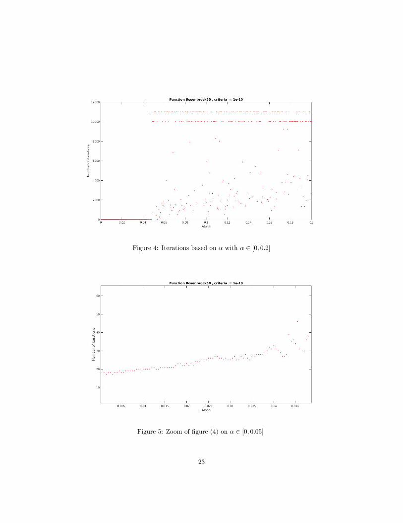
Figure 4: Iterations based on α with α ∈ [0, 0.2]

Figure 5: Zoom of figure (4) on α ∈ [0, 0.05]

23

Figure 6: Iterations based on α with α ∈ [0, 3]

Figure 7: Iterations based on α with α ∈ [0, 0.2]

24

Figure 8: The slowest convergence of MSR1 α ∈ [0, 0.2]

Figure 9: Oscillation of MSR1

25

Figure 10: Example of misleading data

Figure 11: Result showing possible correlation

26

Figure 12: Counter example of a possible correlation

27