IMPROVEMENT OF REVERSE OSMOSISTHROUGH PRETREATMENT--PHASE II

by

Michael K . Stenstrom, Ph .D ., P.E.Associate Professor and Principal Investigator

Report Number UCLA-Eng-83-22Water Resources Program,

School of Engineering and Applied Science,University of California, Los Angeles .

May, 1983

TABLE OF CONTENTSpage

TABLE OF CONTENTS ILIST OF FIGURES tiLIST OF TABLES . . :ACKNOWLEDGEMENTS IvABSTRACT v1 . INTRODUCTION 22. EXPERIMENTAL APPARATUS 4

MEMBRANE CONFIGURATIONS 4PILOT PLANT DESCRIPTION 7CHRONOLOGY OF RO PLANT OPERATION 11ANALYTICAL MEASUREMENTS 19FLUX DECLINE TESTS 21

3. EXPERIMENTAL RESULTS 24FLUX DECLINE AND THE EFFECTS OF CLEANING 24FEED WATER QUALITYFLUX DECLINE AND THE EFFECTS OF PRETREATMENT 29

Flux Decline Tests 30Flux Decline Parameter 34

4. DESIGN ANALYSIS 37FACILITY SIZE 37BASIS FOR COST ESTIMATES 39

5 . CONCLUSIONS 48REFERENCES 50APPENDICES 52

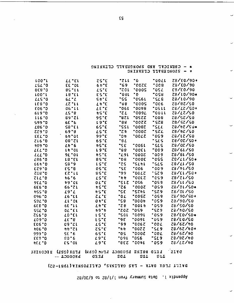
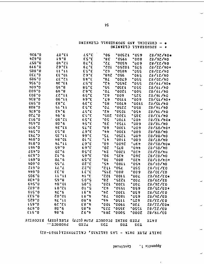
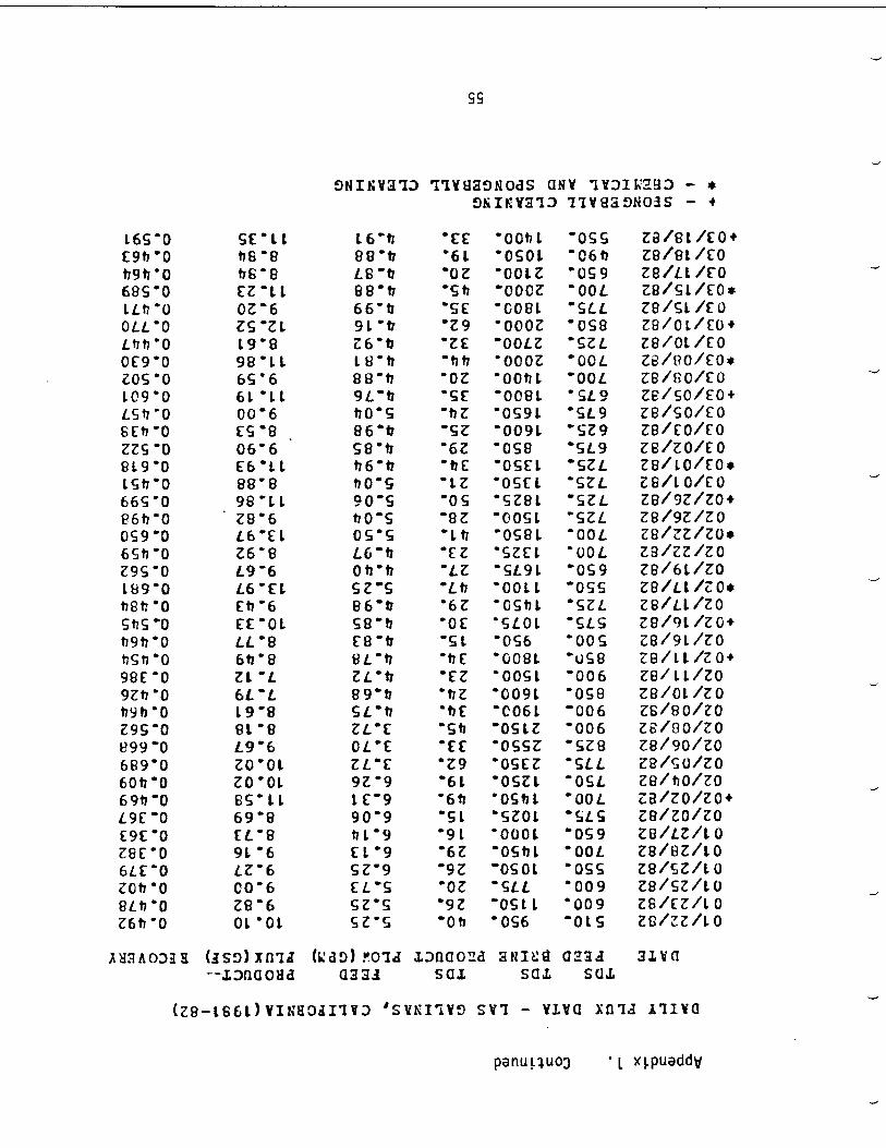
Appendix 1-Data Summary from 1/1/82 to 6/30/82 53Appendix 2-Optimal Reclamation Plant Design from Phase I56Appendix 3-Computer Model Program Listing 59Appendix 4-Sample Data Sheet 77

i

Figure 2 .1 :

Figure 2 .2 :

Figure 2 .3 :

Figure 3 .1 :

Figure 3 .2 :

Figure 3 .3 :

Figure 3 .4 :

LIST OF FIGURESpage

Membrane Cross Section • • • • • • • . • . 8

RO Pilot Plant and Pretreatment Facilities 10

Activated Sludge Plant • • • • • • • • • • • • • • 12

Membrane Fluxes Before and After Cleaning 25

Turbidities as a Function of Time 28

Twenty-Four Hour Flux Decline Tests : Phase I31

48-Hour Flux Decline Tests-Phase II 33

ii

LIST OF TABLES

Table 2 .1 : Reverse Osmosis Unit Specifications 5Table 2 .2 : Comparison of Reverses Osmosis Membrane Configurations6Table 2 .3 : Specifications and Operating Parameters 13Table 2 .4 : Final Membrane Cleaning Procedure 15Table 2 .5 : Chronological Summary of Pilot Plant Operation20Table 3 .1 : Chemical Analysis of RO Feed Water and Product Water27Table 3 .2 : Flux Decline Parameters 35Table 4 .1 : Cost Indices from Various Sources 37Table 4 .2 : Size Variables and Design Basis 41Table 4 .3 : Cost Coefficients for the Log-Linear Functions42Table 4 .4 : Optimal Design for a 1 MGD Facility 43Table 4 .5 : Treatment Cost in Dollars per Thousand Gallons for a 1 MGD . . . . 46

iii

page

ACKNOWLEDGMENTS

The work reported herein was supported by the California Department ofWater Resources under contract numbers B53131 and B54322 . Throughout thestudy a number of individuals helped or provided valuable assistance . Theauthor is especially thankful to the Marin Municipal Water District and theLas Gallinas Valley Sanitary District for providing assistance in the day today operation. Mr. Roger Lindholm and Mr . Darrell Perkins of the CaliforniaDepartment of Water Resources were especially helpful with the administrationand technical support of the project. Mr . Jimmy Lopez, also of the CaliforniaDepartment of Water Resources, maintained the unit, helped with construction,and provided needed support, which is greatly appreciated . Mr. Steven Song,Mr . Hyung Hwang, Mr . Adam Ng, and Mr . John Davis of the UCLA Water QualityLaboratory helped with pilot plant construction and data collection duringparts of the study .

iv

ABSTRACT

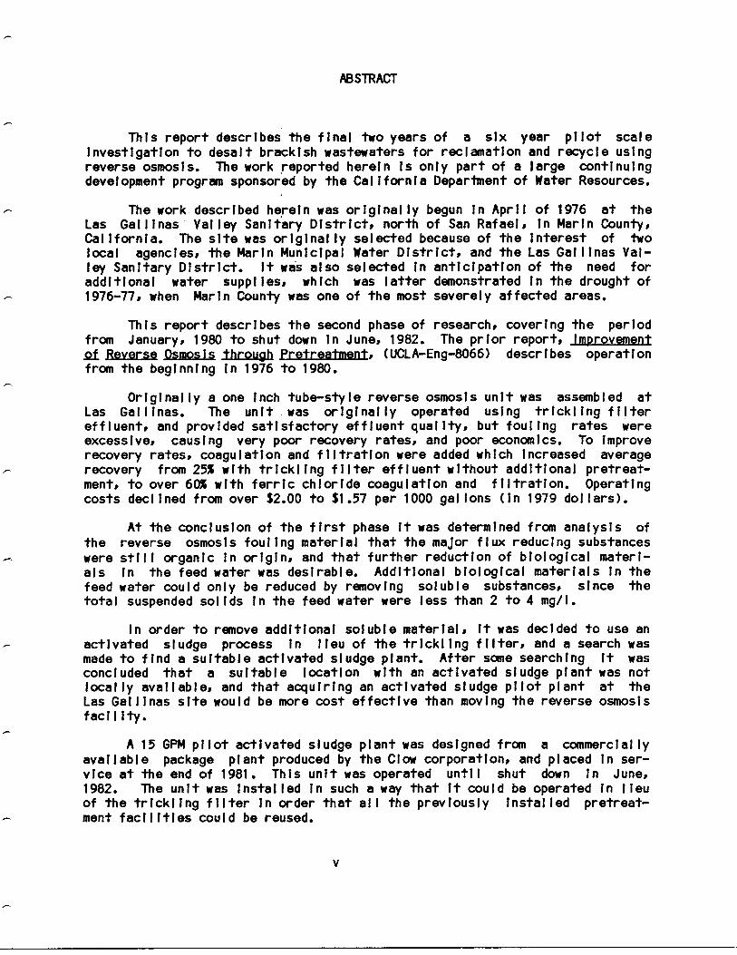
This report describes the final two years of a six year pilot scaleinvestigation to desalt brackish wastewaters for reclamation and recycle usingreverse osmosis . The work reported herein is only part of a large continuingdevelopment program sponsored by the California Department of Water Resources .

The work described herein was originally begun in April of 1976 at theLas Gallinas Valley Sanitary District, north of San Rafael, in Marin County,California. The site was originally selected because of the interest of twolocal agencies, the Marlin Municipal Water District, and the Las Gallinas Val-ley Sanitary District . It was also selected in anticipation of the need foradditional water supplies, which was latter demonstrated in the drought of1976-77, when Mann County was one of the most severely affected areas.

This report describes the second phase of research, covering the periodfrom January, 1980 to shut down in June, 1982 . The prior report, ImprovementQf Reverse Osmosis through Pretreatment, (UCLA-Eng-8066) describes operationfrom the beginning in 1976 to 1980.

Originally a one inch tube-style reverse osmosis unit was assembled atLas Gallinas . The unit was originally operated using trickling filtereffluent, and provided satisfactory effluent quality, but fouling rates wereexcessive, causing very poor recovery rates, and poor economics . To improverecovery rates, coagulation and filtration were added which increased averagerecovery from 25% with trickling filter effluent without additional pretreat-ment, to over 60% with ferric chloride coagulation and filtration. Operatingcosts declined from over $2 .00 to $1 .57 per 1000 gallons (in 1979 dollars) .

At the conclusion of the first phase it was determined from analysis ofthe reverse osmosis fouling material that the major flux reducing substanceswere still organic in origin, and that further reduction of biological materi-als in the feed water was desirable . Additional biological materials in thefeed water could only be reduced by removing soluble substances, since thetotal suspended solids in the feed water were less than 2 to 4 mg/l .

In order to remove additional soluble material, it was decided to use anactivated sludge process in lieu of the trickling filter, and a search wasmade to find a suitable activated sludge plant . After some searching it wasconcluded that a suitable location with an activated sludge plant was notlocally available, and that acquiring an activated sludge pilot plant at theLas Gallinas site would be more cost effective than moving the reverse osmosisfacility .

A 15 GPM pilot activated sludge plant was designed from a commerciallyavailable package plant produced by the Clow corporation, and placed in ser-vice at the end of 1981 . This unit was operated until shut down in June,1982 . The unit was installed in such a way that it could be operated in lieuof the trickling filter in order that all the previously installed pretreat-ment facilities could be reused .

V

The activated sludge plant provided additional organic material removalwhich reduced fouling and operating cost. The cost for the best activatedsludge pretreatment system (activated sludge followed by filtration withoutchemical addition) was $1 .11 per 1000 gallons which can be compared to $1 .57per 1000 gallons for lowest cost from the previous phase, using tricklingfilter effluent followed by ferric chloride coagulation, sedimentation, andfiltration, in 1979 dollars . In first quarter 1983 dollars the cost comparisonwas $1 .71 to $2 .42 per 1000 gallons in favor of the activated sludge treatmentsystem . In all cases the lowest cost operation was obtained with the highestlevel of pretreatment. Aluminum sulfate was always the poorest coagulant inreducing fouling properties of the feed water, but not always the poorestcoagulant in reducing feed water turbidity .

1. INTRODUCTION

In an effort to develop future water resources for the state of Califor-

nia, the California Department of Water Resources (DWR) and others have funded

a series of projects to develop technology to reclaim water from wastewater

discharges. The development of additional water resources from wastewaters is

one method of meeting the future water needs while reducing wastewater

discharge problems . Previous projects have been described by Antoniuk and

McCutchan (1973) and Speight and McCutchan (1979) for irrigation drainage

wastewaters, by Argo and Moutes (1979), Wojcik, Lopez, and McCutchan (1980),

and Stenstrom et. al . (1982a, 1982b) for domestic wastewaters, and by Johnson

and Loeb (1969), Johnson, McCutchan, and Bennion (1969) for saline groundwa-

ters . Other work has also been performed, and the review by Davis, et. al .

(1980) should be consulted for additional information .

This report describes the Phase II results for the research facility

located at the Las Gallinas Valley Sanitary District, north of San Rafael, in

Marin County, California. The objective of the Phase 11 study was to further

investigate pretreatment techniques and their effect on system preformance and

cost, by adding an activated sludge plant . In the Phase I the economics and

system design of a pilot scale tubular reverse osmosis plant treating coagu-

lated and filtered trickling filter effluent were investigated . The Phase I

work, through extensive investigation of coagulation/filtration techniques,

including coagulation by organic polymers, ferric chloride, alum (aluminum

sulfate), showed that pretreatment significantly reduced total costs . It was

concluded from Phase I that total operating cost could be reduced from over

$2 .00 to $1 .57 per 1000 gallons by employing optimum coagulation-filtration

2

pretreatment, as compared to trickling filter effluent without additional

treatment. Additionally the fouling materials removed from the RO membranes

appeared to be organic materials, indicating that additional improvements in

biological pretreatment, such as those provided by an activated sludge plant,

would be beneficial .

This report describes the results of the second phase of research, using

improved pretreatment provided by a pilot scale activated sludge plant,

including revised system economics, followed by various filtration/coagulation

alternatives . In writing this report no attempt was made to discuss results

from the first phase, unless they were essential to interpret the results from

the second phase .

3

2. EXPERIMENTAL APPARATUS

The reverse osmosis apparatus used in this study was the same as that

used in the first phase of work at Las Gallinas and very similar to the units

used in earlier investigations conducted by UCLA researchers (Johnson and

Loeb, 1966; Johnson, et. al . 1969; Speight and McCutchan, 1979) . The unit is

very similar to the original design by Loeb and SouriraJan (1960, 1962). Table

2 .1 lists the specifications for the unit .

MEMBRANE CONFIGURATIONS

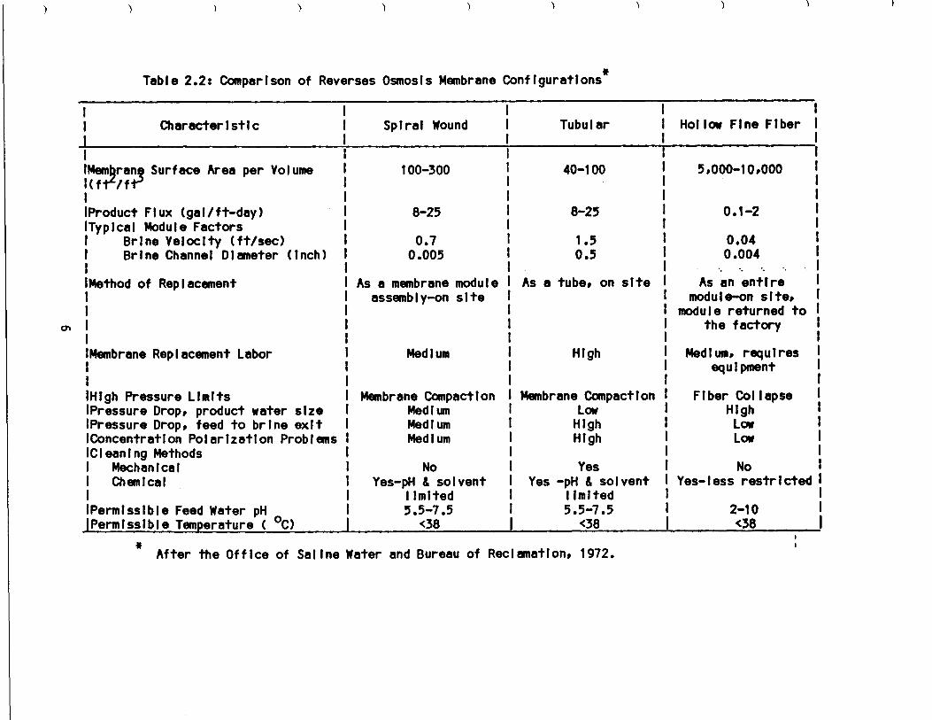
There are three common membrane configurations used today . Each has

advantages and disadvantages. The tubular membranes used in this study have

the advantage of high flux rates, ease of cleaning, and simplicity . Unfor-

tunately they have very low packing density . Spiral wound membranes have much

higher packing density, but are more complicated to manufacture and often have

lower fluxes . Hollow fine fiber membranes have the highest packing density,

but are restricted in application to high quality feed water since they cannot

be easily cleaned . Suspended solids are particularly bothersome and must be

removed from feed water . Table 2 .2 , taken from the the Desaitina Handbook

. Planners (Office of Saline Water, 1972), summarizes the advantages of each

membrane type .

The tube style membranes have been used throughout the UCLA research

projects in part because they allow for membrane development and testing

without requiring extensive equipment and facilities . All the membranes used

in both phases of this study were cast by DWR personnel at their Firebaugh,

California facility . The tube style membranes are particularly useful in

4

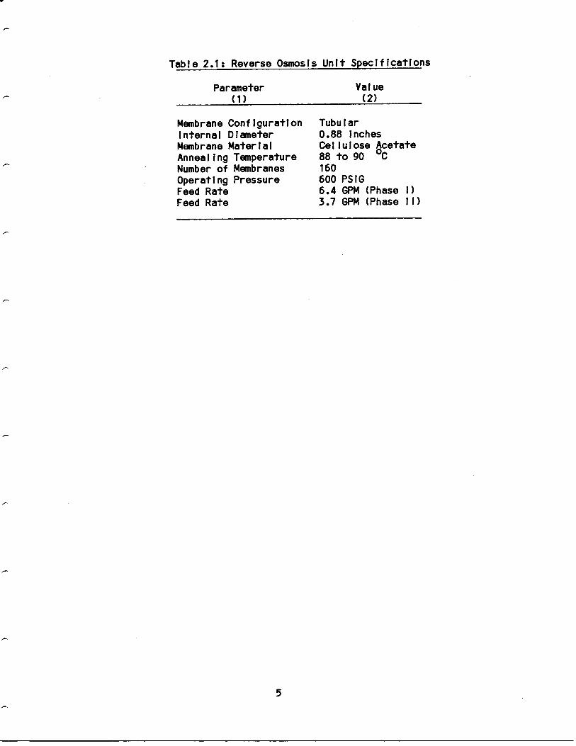
Table 2 .1 : Reverse Osmosis Unit Specifications

Parameter(1)

Membrane ConfigurationInternal DiameterMembrane MaterialAnnealing TemperatureNumber of MembranesOperating PressureFeed RateFeed Rate

5

Value(2)

Tubular0 .88 inchesCellulose Acetate88 to 90 °C160600 PSIG6.4 GPM (Phase 1)3 .7 GPM (Phase II)

rn

I

Table 2 .2 : Comparison of Reverses Osmosis Membrane Configurations *

Characteristic

Mem ran Surface Area per VolumeI(ftL/ftJIProduct Flux (gal/ft-day)Typical Module Factors

Brine Velocity (ft/sec)Brine Channel Diameter (inch)

Method of Replacement

Membrane Replacement Labor

(High Pressure Limits(Pressure Drop, product water sizelPressure Drop, feed to brine exitConcentration Polarization ProblemsCleaning Methods

MechanicalChemical

*After the Office of Saline

Spiral Wound

100-300

8-25

0 .70 .005

As a membrane moduleassembly-on site

Medium

Membrane CompactionMediumMediumMedium

Tubular

40-100

8-25

1 .50 .5

As a tube, on site

High

Membrane CompactionLowHighHigh

Water and Bureau of Reclamation, 1972 .

1

Hollow Fine Fiber

5,000-10,000

0 .1-2

0 .040 .004

As an entiremodule-on site,

module returned tothe factory

Medium, requiresequipment

Fiber CollapseHighLowLow

NoYes-less restricted

No

YesYes-pH & solvent

Yes -pH & solventlimited

limitedPermissible Feed Water pH

5 .5-7 .5

5.5-7 .5

2-10Permissible Temperature(°C)I<38(<38I<38

1

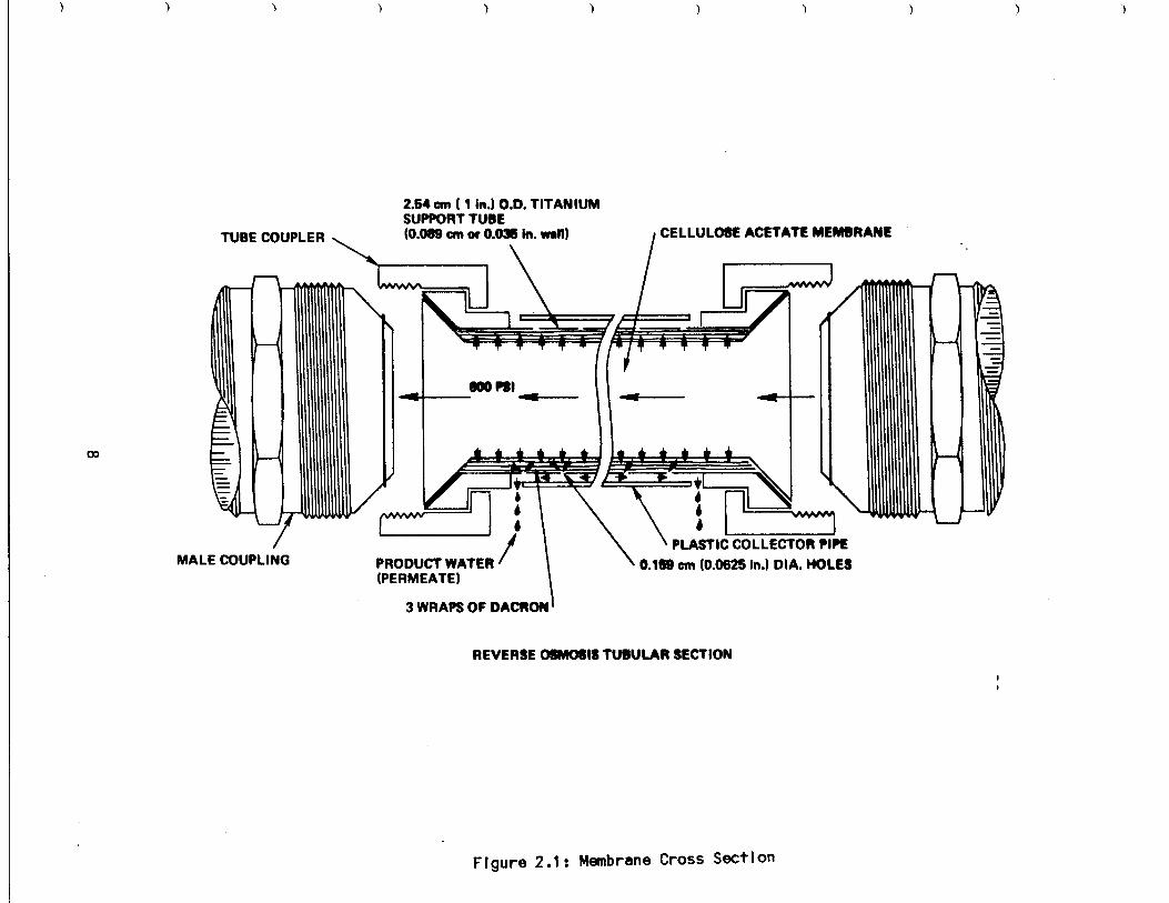
reclamation studies since they can be used with the largest range of feed

water qualities . Figure 2 .1 shows a cross section of the membrane configura-

tion used at Las Gallinas . Each membrane is 0 .88 inches in diameter and ten

feet long, providing a total surface area of 2 .24 ft2 . The entire RO unit

contained 160 membranes, for a total area of 358 ft2 .

PILOT PLANT DESCRIPTION

The pilot plant was located at the Las Gallinas Valley Sanitary District

north of San Rafael, California . The District operates a secondary treatment

plant composed of primary clarification, two stage trickling filters, and

secondary clarification . The flow rate to the plant ranges from the average

value of 1 .5 MGD (0 .065 m3/sec) to upwards of 8 MGD (0 .35 m3/sec) in wet

weather . The trickling filters are loaded at a rate of 11 MGD/acre (1,17 x

10-4m3 /m2-sec) and 84 pounds of five-day biochemical oxygen demand (BOD 5) per

thousand cubic feet of filter media (1 .35 kg BOD5/m3 ) . This loading is con-

sidered to be a high loading rate according to current design standards, and

at this loading rate the filters are expected to produce effluent BOD 5 ranging

from 12 to 25 mg/l, and should not nitrify . (Reynolds, 1982, Metcalf and

Eddy, 1979) . This effluent BOO5 concentration compares to 5 to 15 mg/I to be

expected from a well designed and operated activated sludge plant(Metcalf and

Eddy, 1979) .

The Las Gallinas plant showed fluctuations in treatment efficiency

depending on season . In the winter the effluent was visibly poorer than sum-

mer effluent, with turbidities exceeding 20 NTU on occasions . The decrease in

effluent quality in winter can be primarily attributed to the increase in

7

w

1

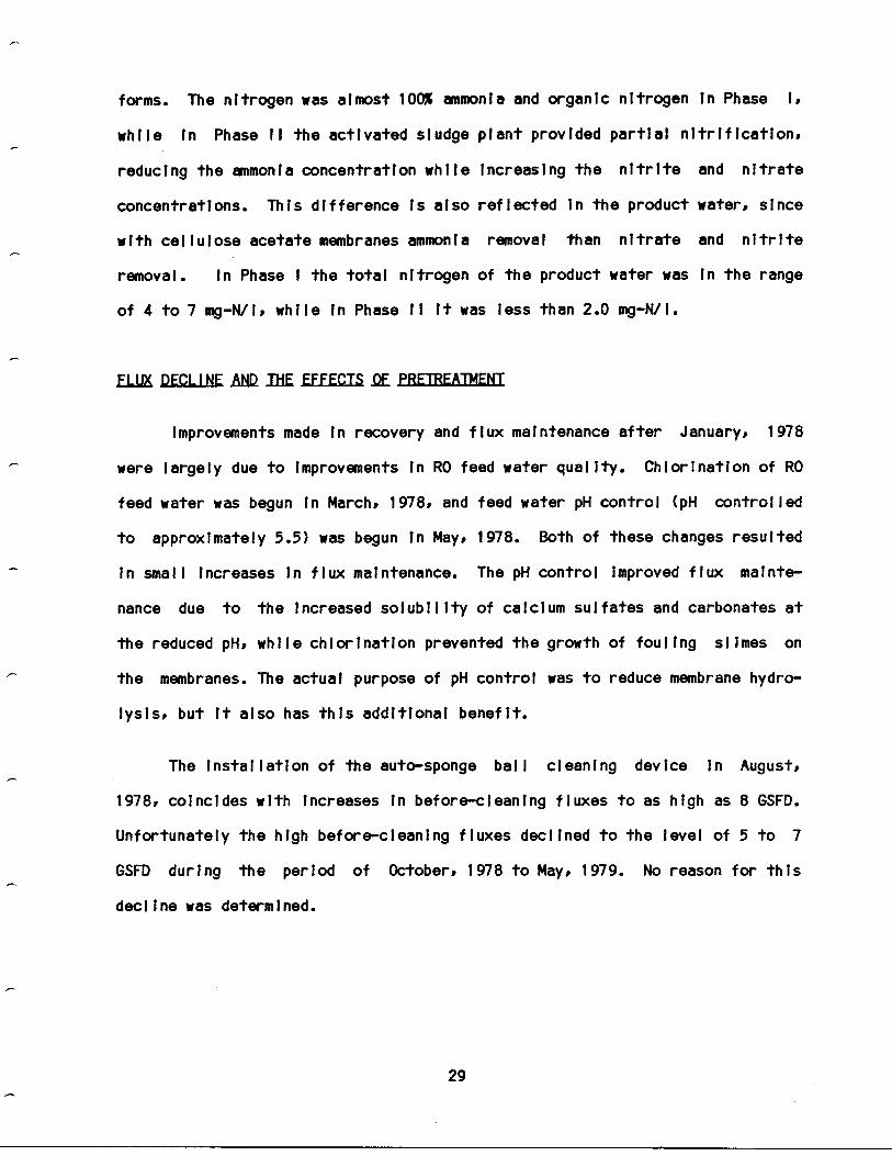
TUBE COUPLER

MALE COUPLING

2.54 cm (1 in .) O.D. TITANIUMSUPPORT TUBE(0.089 cm or 0.038 in . wall)

111

PRODUCT WATER(PERMEATE)

3 WRAPS OF DACRON

REVERSE OSMOSIS TUBULAR SECTION

CELLULOSE ACETATE MEMBRANE

11

PLASTIC COLLECTOR PIPE

0.159 cm (0.0625 in.) DIA. HOLES

Figure 2 .1 : Membrane Cross Section

0

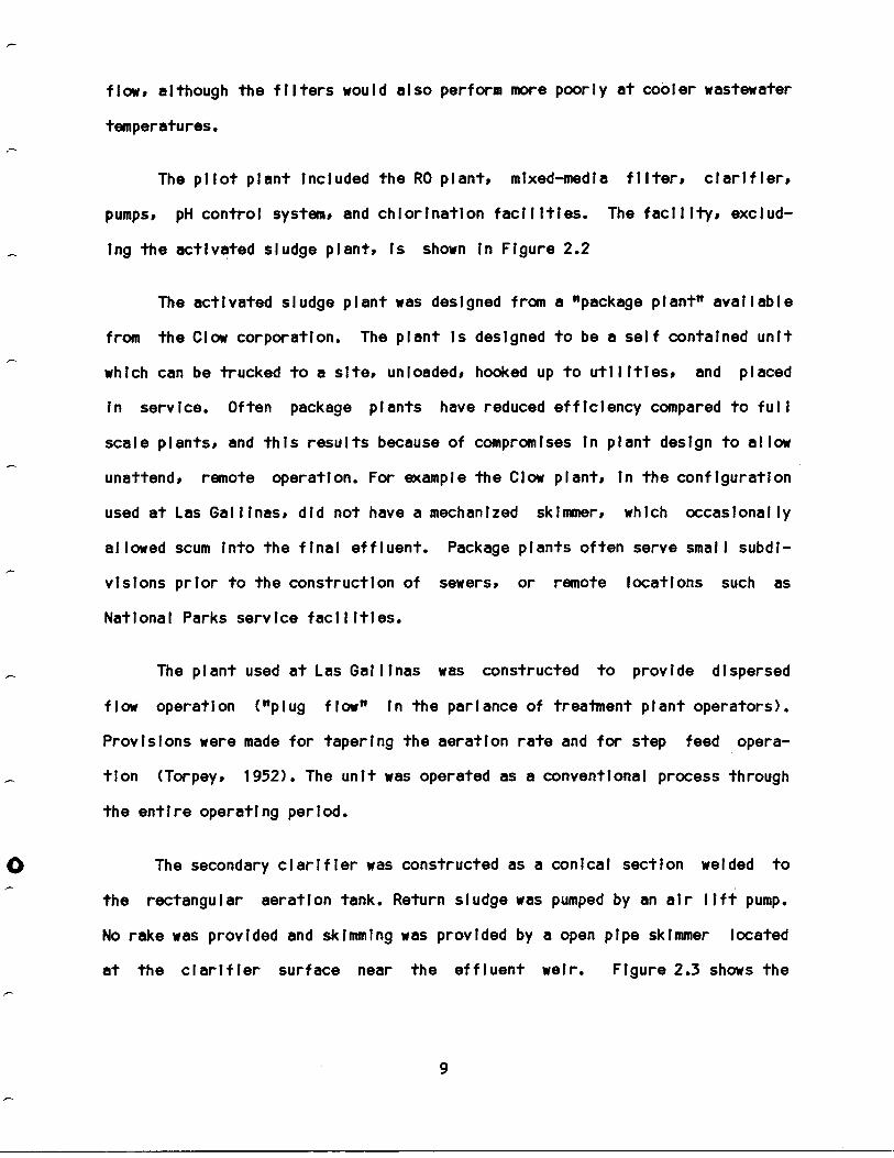
flow, although the filters would also perform more poorly at cooler wastewater

temperatures.

The pilot plant included the RO plant, mixed-media filter, clarifier,

pumps, pH control system, and chlorination facilities . The facility, exclud-

ing the activated sludge plant, is shown in Figure 2 .2

The activated sludge plant was designed from a "package plant" available

from the Clow corporation . The plant is designed to be a self contained unit

which can be trucked to a site, unloaded, hooked up to utilities, and placed

in service . Often package plants have reduced efficiency compared to full

scale plants, and this results because of compromises in plant design to allow

unattend, remote operation . For example the Clow plant, in the configuration

used at Las Gallinas, did not have a mechanized skimmer, which occasionally

allowed scum into the final effluent. Package plants often serve small subdi-

visions prior to the construction of sewers, or remote locations such as

National Parks service facilities .

The plant used at Las Gallinas was constructed to provide dispersed

flow operation ("plug flow" in the parlance of treatment plant operators) .

Provisions were made for tapering the aeration rate and for step feed opera-

tion (Torpey, 1952) . The unit was operated as a conventional process through

the entire operating period .

The secondary clarifier was constructed as a conical section welded to

the rectangular aeration tank . Return sludge was pumped by an air lift pump .

No rake was provided and skimming was provided by a open pipe skimmer located

at the clarifier surface near the effluent weir .

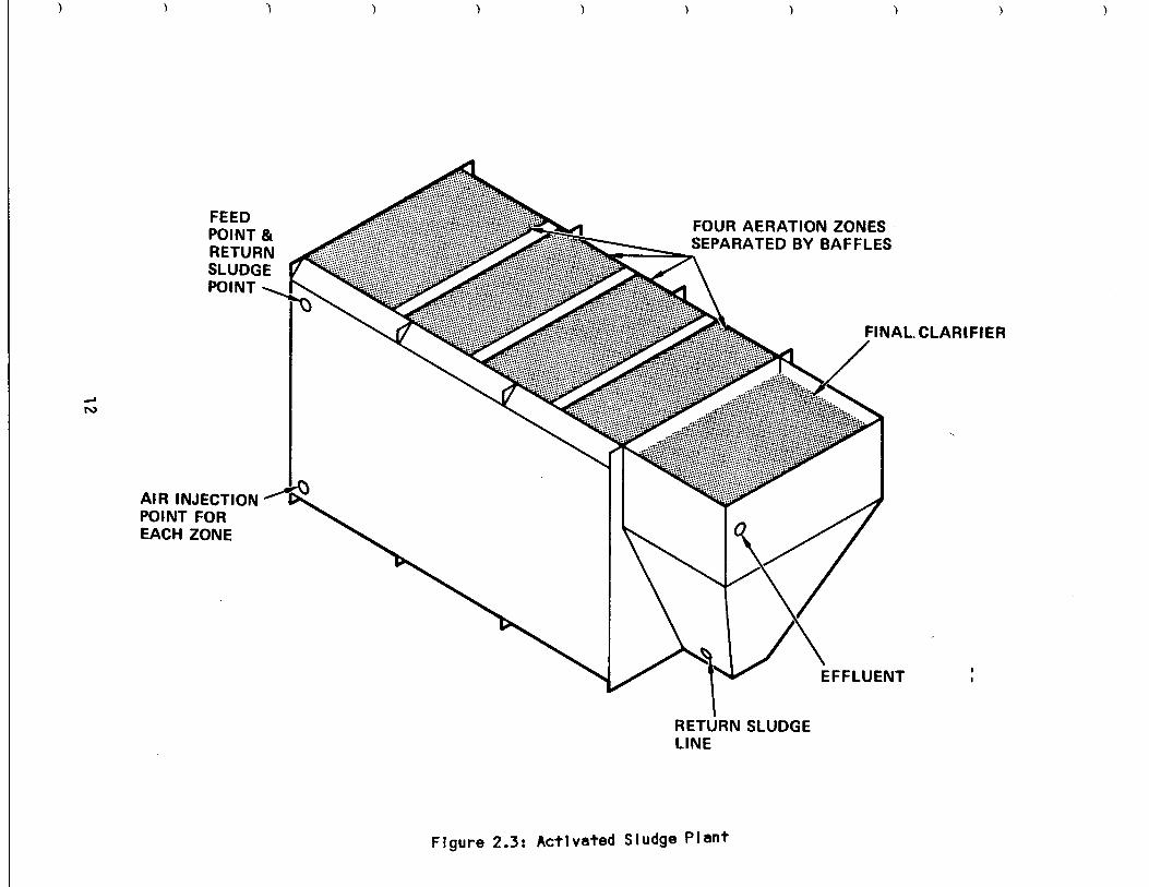
Figure 2 .3 shows the

9

JO

10

)

)

)

12 • 77

Figure 2 .2 : RO Pilot Plant and Pretreatment Facilities

0

RO UNIT

1. FEEDWATER SECONDARY EFFLUENT2. CLARIFIER INFLUENT3. DIRECT FILTRATION BYPASS VALVE4. CLARIFIER EFFLUENT5. SLUDGE TO DISPOSAL

C-~6. MIXED-MEDIA FILTER INFLUENT

7. FILTER EFFLUENT8. RO INFLUENT HIGH

PRESSUREFLOW

PUMPREVERSE

9. BRINE TO DISPOSAL

C10. RO PRODUCT WATER

)11. CHEMICAL ADDITION POINT12. FILTER SURFACE WASH AND BACKWASH13. BACKWASH TO DISPOSAL VALVE14. CHLORIDE INJECTION POINT15 .

ACIDINJECTION

30 MICRON FILTERTO PROTECT PUMP

RO FEEDWATERSTORAGE

13(7.6m3)J C

15MIXEDMEDIAFILTER 14(0.61 m d1a.)

BACKWASH ANDU RO FEEDWATERSTORAGE(3.21 m3 )

activated sludge plant . The specifications and operating parameters for the

plant are described in Table 2.3 .

The filter was constructed from a 24 inch section of low carbon steel

pipe, and was equipped with a rock underdrain structure and mixed media . The

filter media used was a commercially available media (Neptune-Microfloc) con-

sisting of a 1 .0 to 1 .2 mm size distribution of coal, a 0 .42 to 0 .55 mm size

distribution of silica sand, and a 0 .2-0 .3 mm size distribution of garnet

sand . The filter was backwashed using a hydraulic surface wash in addition to

a normal backwash which fluidized the entire filter media .

CHRONOLOGY QE $Q PLANT OPERATION

The RO pilot plant was originally placed In operation in April, 1976

treating trickling filter influent which was filtered through a 30 inch diame-

ter multi-media (sand and coal) filter. This filter, besides providing feed

for the RO unit, was operated by the Marin Municipal Water District (MMWD) to

provide water for their reclamation activities . The RO unit operated on fil-

tered trickling filter effluent from the Mann filter until May of 1979 when

the 24 inch diameter mixed-media filter was installed and dedicated to pre-

treatment of RO feed water .

The initial period from April, 1976 to June, 1979 was dedicated to the

development of membrane cleaning techniques and endurance testing of the RO

membranes and equipment . The original cleaning technique was restricted to

sponge ball cleaning without chemical cleaning agents (sponge ball cleaning

was developed earlier by McCutchan and co-workers, and uses a sphere of flexi-

ble plastic or rubber which Is forced along the tubular membranes by the brine

1 1

FEEDPOINT &RETURNSLUDGEPOINT

AIR INJECTIONPOINT FOREACH ZONE

Figure 2 .3 : Activated Sludge Plant

FOUR AERATION ZONESSEPARATED BY BAFFLES

. FINAL. CLARIFIER

RETURN SLUDGELINE

Table 2 .3 : Specifications and Operating Parametersfor the Activated Sludge Plant .

Parameter(1)

Hydraulic RetentionTime at 12 GPM

Overflow rate at12 GPM

Mean Cell RetentionTime

* 12 GPM = 0 .045 m3/min

1 3

Value(2)

10 .4 hours

480 gal/ft2day (4 .9 m/day)

5 days

Aeration SectionDepthLengthWidthVolume

9 ft (2 .75m)14 ft (4 .25m)8 ft (2 .43

7500 gal (28 .4

)

Clarifier SectionDepth 9 ft (2 .75 m)Length 4 .5 ft (1 .37 m)Width 8 ft (2 .43 )Volume 1450 a al (5 .5 ~)Surface Area 36 ft' (13.3

)

or wash water pressure) . During cleaning the unit was always depressurized and

flushed with tap water or RO product water (later containing cleaning chemi-

cals) . Beginning in April of 1977 a two hour enzyme detergent flush was ini-

tiated . In June of 1977 the detergent flush was stopped and a citric acid

flush was begun . Combinations of cleaning techniques were evaluated until

March, 1978, when a final cleaning procedure, consisting of one hour flushes

with citric acid and detergent followed by sponge ball cleaning, was

developed . Table 2 .4 summarizes the final cleaning procedure .

In March, 1978, chlorination of RO feed water was begun and in May of

1978 pH control of feed water was started . Operation continued in this fashion

until June, 1979, when improved pretreatment facilities were placed in ser-

vice.

From June until July, 1979 feed water was pretreated using direct fil-

tration with a cationic organic polymer (Nalco 7134) . In July, 1979 a 5 .5 ft

(1 .7 m) diameter clarifier was installed and inorganic coagulants were used .

At this time a protocol for operating the mixed-media filter was developed and

continued throughout the remainder of the study . The filter was operated at

3 .2 GPM/ft2 (2 .17 I/m2 sec) filtration rate and backwashed at 18-20 GPM/ft 2

(10 .2-13 .6 I/m2 ) for five minutes after a two minute surface wash . Backwash-

ing was performed automatically on a timed cycle . Usually backwashes were per-

formed every 12 hours . The filter was operated at the 3 .2 GPM/ft2 (2 .17 I/m2 )

rate independently of the RO feed water rate in order to provide uniform

operation . Excess feed water was discharged with the Las Gallinas Valley San-

itary District effluent .

1 4

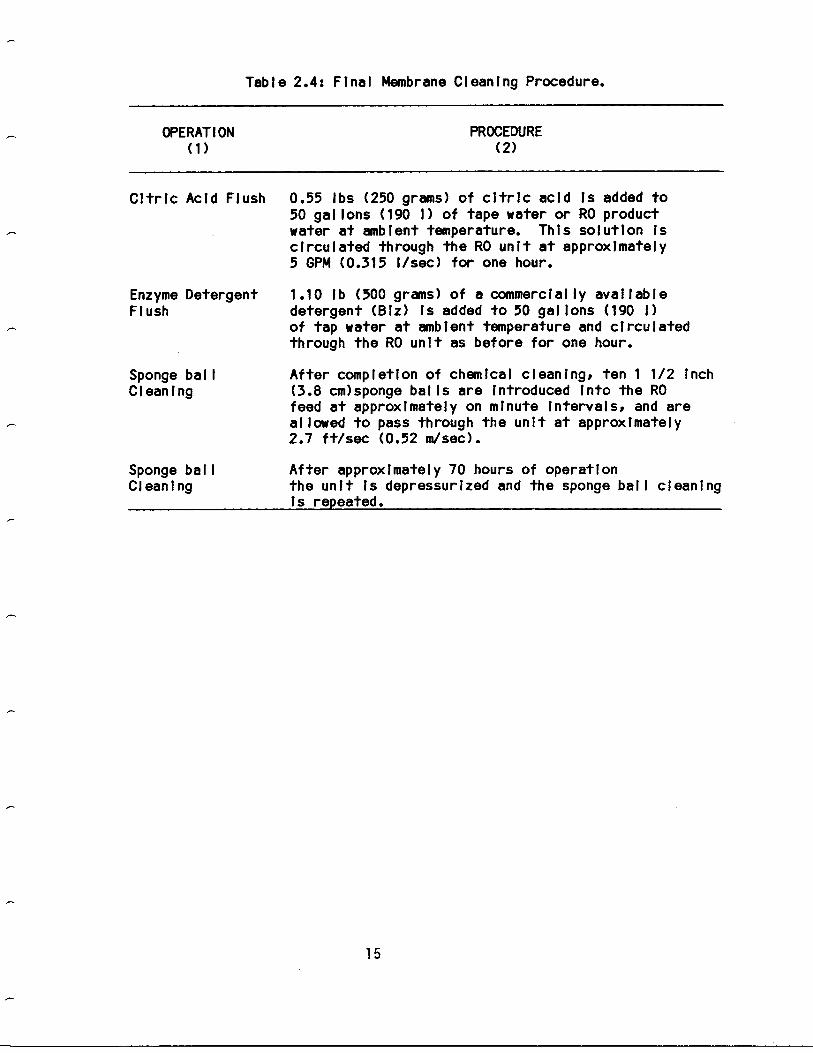
Table 2 .4 : Final Membrane Cleaning Procedure .

OPERATION

PROCEDURE(1)

(2)

Citric Acid Flush 0 .55 lbs (250 grams) of citric acid is added to50 gallons (190 I) of tape water or RO productwater at ambient temperature . This solution iscirculated through the RO unit at approximately5 GPM (0 .315 I/sec) for one hour .

Enzyme Detergent

1 .10 lb (500 grams) of a commercially availableFlush

detergent (Biz) is added to 50 gallons (190 I)of tap water at ambient temperature and circulatedthrough the RO unit as before for one hour .

Sponge ball

After completion of chemical cleaning, ten 1 1/2 InchCleaning

(3.8 cm)sponge balls are introduced Into the ROfeed at approximately on minute intervals, and areallowed to pass through the unit at approximately2 .7 ft/sec (0 .52 m/sec) .

Sponge ball

After approximately 70 hours of operationCleaning

the unit is depressurized and the sponge ball cleaningis repeated .

1 5

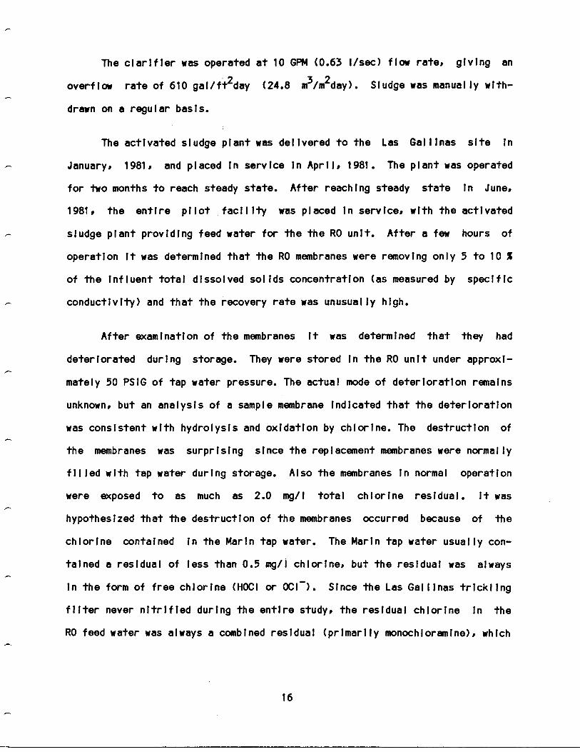
The clarifier was operated at 10 GPM (0 .63 I/sec) flow rate, giving an

overflow rate of 610 gal/ft2day (24.8 m3/m2day) . Sludge was manually with-

drawn on a regular basis .

The activated sludge plant was delivered to the Las Gallinas site in

January, 1981, and placed in service in April, 1981 . The plant was operated

for two months to reach steady state . After reaching steady state in June,

1981, the entire pilot facility was placed in service, with the activated

sludge plant providing feed water for the the RO unit . After a few hours of

operation it was determined that the RO membranes were removing only 5 to 10 %

of the influent total dissolved solids concentration (as measured by specific

conductivity) and that the recovery rate was unusually high .

After examination of the membranes it was determined that they had

deteriorated during storage . They were stored in the RO unit under approxi-

mately 50 PSIG of tap water pressure . The actual mode of deterioration remains

unknown, but an analysis of a sample membrane indicated that the deterioration

was consistent with hydrolysis and oxidation by chlorine . The destruction of

the membranes was surprising since the replacement membranes were normally

filled with tap water during storage . Also the membranes in normal operation

were exposed to as much as 2 .0 mg/I total chlorine residual . It was

hypothesized that the destruction of the membranes occurred because of the

chlorine contained in the Mar in tap water . The Marin tap water usually con-

tained a residual of less than 0 .5 mg/I chlorine, but the residual was always

in the form of free chlorine (HOCI or OCI ) . Since the Las Gallinas trickling

filter never nitrified during the entire study, the residual chlorine in the

RO feed water was always a combined residual (primarily monochloramine), which

16

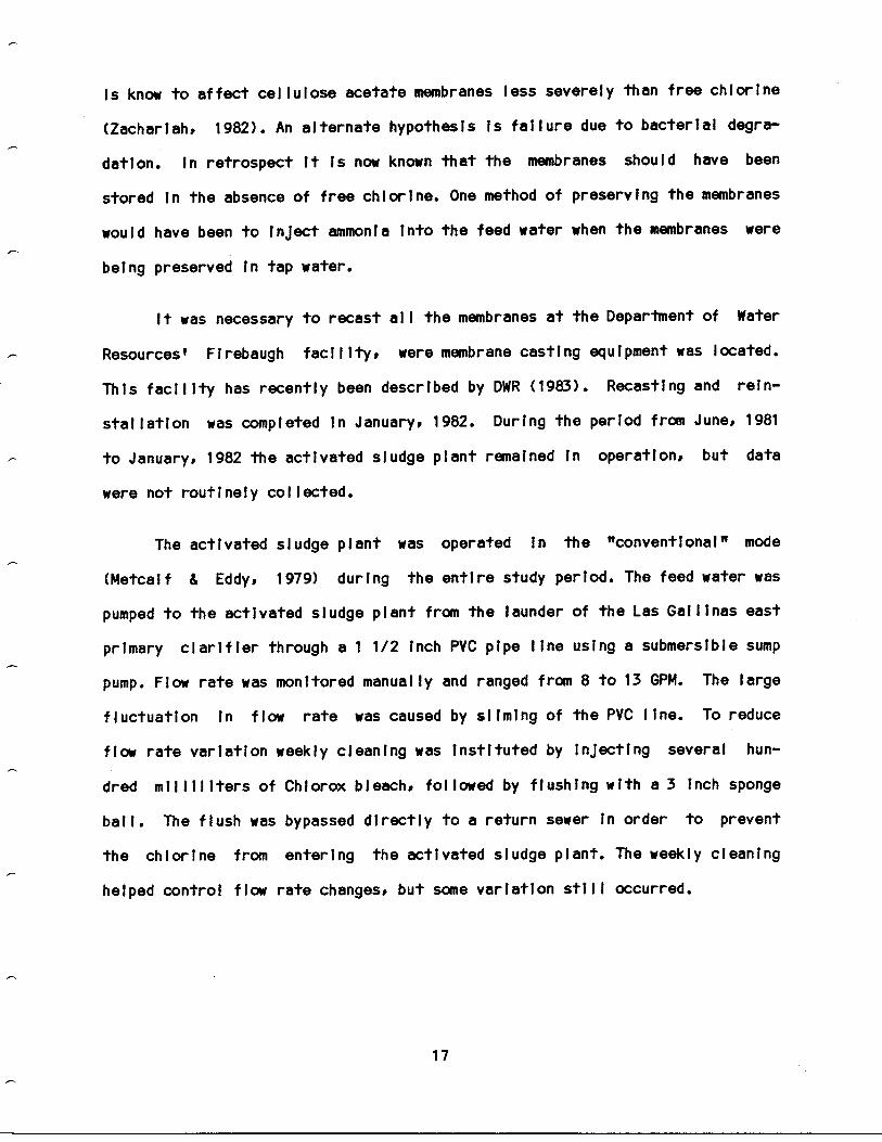
is know to affect cellulose acetate membranes less severely than free chlorine

(Zachariah, 1982) . An alternate hypothesis is failure due to bacterial degra-

dation . In retrospect it is now known that the membranes should have been

stored in the absence of free chlorine . One method of preserving the membranes

would have been to inject ammonia into the feed water when the membranes were

being preserved in tap water .

It was necessary to recast all the membranes at the Department of Water

Resources' Firebaugh facility, were membrane casting equipment was located .

This facility has recently been described by DWR (1983) . Recasting and rein-

stallation was completed in January, 1982 . During the period from June, 1981

to January, 1982 the activated sludge plant remained in operation, but data

were not routinely collected .

The activated sludge plant was operated in the "conventional" mode

(Metcalf & Eddy, 1979) during the entire study period . The feed water was

pumped to the activated sludge plant from the launder of the Las Gallinas east

primary clarifier through a 1 1/2 inch PVC pipe line using a submersible sump

pump . Flow rate was monitored manually and ranged from 8 to 13 GPM . The large

fluctuation in flow rate was caused by sliming of the PVC line . To reduce

flow rate variation weekly cleaning was instituted by injecting several hun-

dred milliliters of Chlorox bleach, followed by flushing with a 3 inch sponge

ball . The flush was bypassed directly to a return sewer in order to prevent

the chlorine from entering the activated sludge plant . The weekly cleaning

helped control flow rate changes, but some variation still occurred .

1 7

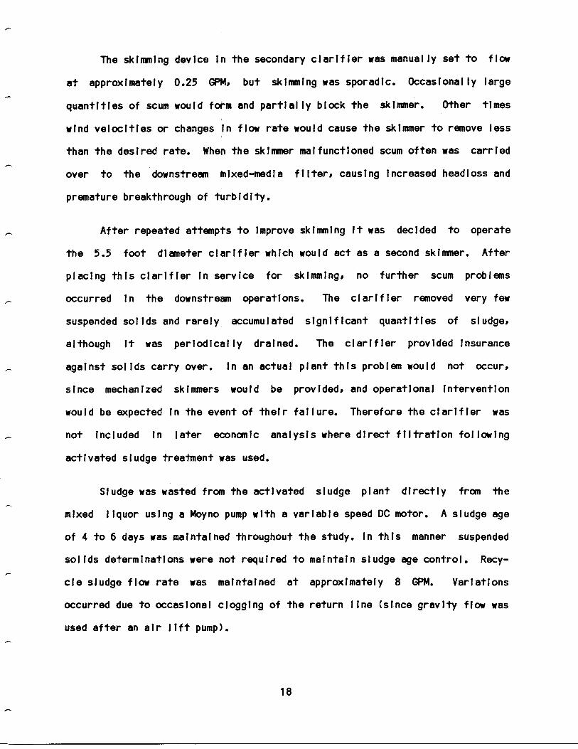
The skimming device in the secondary clarifier was manually set to flow

at approximately 0 .25 GPM, but skimming was sporadic . Occasionally large

quantities of scum would form and partially block the skimmer. Other times

wind velocities or changes in flow rate would cause the skimmer to remove less

than the desired rate. When the skimmer malfunctioned scum often was carried

over to the downstream Mixed-media filter, causing increased headloss and

premature breakthrough of turbidity .

After repeated attempts to improve skimming it was decided to operate

the 5 .5 foot diameter clarifier which would act as a second skimmer . After

placing this clarifier in service for skimming, no further scum problems

occurred in the downstream operations . The clarifier removed very few

suspended solids and rarely accumulated significant quantities of sludge,

although it was periodically drained . The clarifier provided insurance

against solids carry over . In an actual plant this problem would not occur,

since mechanized skimmers would be provided, and operational intervention

would be expected in the event of their failure . Therefore the clarifier was

not included in later economic analysis where direct filtration following

activated sludge treatment was used .

Sludge was wasted from the activated sludge plant directly from the

mixed liquor using a Moyno pump with a variable speed DC motor . A sludge age

of 4 to 6 days was maintained throughout the study. In this manner suspended

solids determinations were not required to maintain sludge age control . Recy-

cle sludge flow rate was maintained at approximately 8 GPM . Variations

occurred due to occasional clogging of the return line (si-nce gravity flow was

used after an air lift pump) .

1 8

It is useful to compare the activated sludge plant operation at the Las

Gallinas test site to a typical full scale activated sludge plant . The Las

Gallinas pilot plant did not receive as much operational attention as would be

expected at a well operated full scale facility . The effluent turbidities for

the pilot plant were more than the effluent turbidities routinely obtained at

the activated sludge plants operated by the City of Los Angeles or Los Angeles

County Sanitation Districts . This difference might be in part due to cooler

operating temperatures at Las Gallinas . In contrast to most plants the Las

Gallinas plant did not receive diurnal flow variation . The clarifier in the

pilot plant did not operate as efficiently as a full scale clarifier, which

was attributed to the lack of mechanical skimmer and rake . One would expect a

full scale facility to provide equal or better quality effluent than the pilot

plant .

Table 2 .5 summarizes the period of operation and timing of significant

events . Throughout the entire period of-operation the units were maintained

almost without day-to-day manual supervision . Perhaps 0 .5 to 1 .5 hours per day

were spent on maintenance and operation (with the exception of membrane clean-

ing), and most of this time was spent data logging and mixing coagulants .

ANALYTICAL MEASUREMENTS

Most of the analytical work was performed on site using the existing

laboratory facilities . Turbidities were measured with a Turner Designs Model

40-005 turbidity meter . Flow rates were usually measured by clocking flows

into vessels of known volume . Extensive analyses of the influent and effluent

water quality parameters were performed periodically by the Department of

1 9

)

Table 2 .5 : Chronological Summary of Pilot Plant Operation .

1Date

Hour(1)

(2)~

EventI

(3)Comment

(4)

4/27/76

0 I Pilot plant started up on trickling filter j Weekly sponge ball cleaning without

4/18/77

8,500

i effluent after multi-media filtration .II Cleaning procedure changed by the addition

I chemicalsII Various concentrations of detergent

6/20/77 10,000

I of two hour enzyme detergent flush . I (up to 2 .1 g/1) were used for flushing .

Concentrations between 0 .04 andII Citric Acid substituted for enzyme detergent

9/26/77 12,400

III Returned to enzyme detergent

0 .53 g/I were used

Concentrations between 1 .05 and .32 g/I

1/1/78

14,700

III Final cleaning procedure developed, using

were used .

0.66 g/I citric acid concentrationI one hour citric acid flush, followed by oneI hour enzyme detergent flush, followed byI sponge ball cleaning

1

and 1 .32 g/I enzyme used for flush

3/23/78 16,700 i Chlorination of multl-media filter effluent begun Chlorine residual ranged from 0.5NC) 1 I 1 to 6.0 mg/I, averaging 2.0 mg/1 .

I

1 15/15/78 I 18,000 t Influent pH control Initiated by addition I set point at pH-5 .5

1 of sulfuric acid

18/1/78

19,800 I Automatic sponge ball cleaning started Cleaning frequency set at six hoursI

6/1/79

27,100 I Mixed-media filter cationic polymer coagulation Dosage set by ZetaI Initiated

I7/6/79

28,000 I Clarifier Installed and operation with various

I potential measurements

IOptimal concentrations of

I coagulants and modes until shut down

1/7/80 132,400 Unit shut down .

4/1/81

43,200 1 Activated sludge plant started up

6/1/81

44,600 RO unit started up and shut down

1/22/82 49,400 RO restarted using activated sludge plantI

I as feed water

6/23/82 j 53,000 Unit shut down and disassembled

FOCI3#

A1 2(S04 ) 3 evaluated .

Membranes stored under pressurized tap water

Membranes destroyed

Operated with various coagulantsuntil shut down

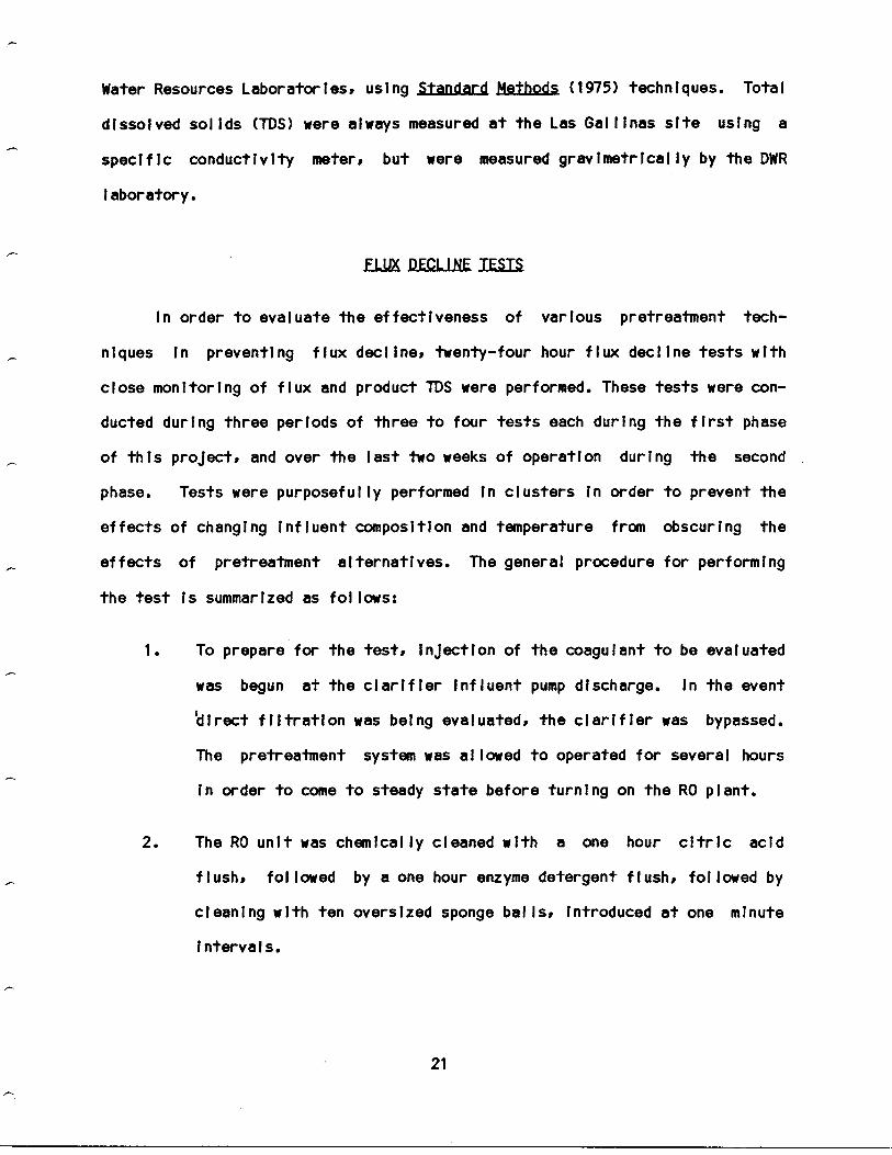
Water Resources Laboratories, using Standard .Methods (1975) techniques. Total

dissolved solids (TDS) were always measured at the Las Gallinas site using a

specific conductivity meter, but were measured gravimetrically by the DWR

laboratory .

FLUX DECLINE TESTS

In order to evaluate the effectiveness of various pretreatment tech-

niques In preventing flux decline, twenty-four hour flux decline tests with

close monitoring of flux and product TDS were performed . These tests were con-

ducted during three periods of three to four tests each during the first phase

of this project, and over the last two weeks of operation during the second

phase . Tests were purposefully performed in clusters in order to prevent the

effects of changing influent composition and temperature from obscuring the

effects of pretreatment alternatives . The general procedure for performing

the test is summarized as follows :

1 . To prepare for the test, Injection of the coagulant to be evaluated

was begun at the clarifier influent pump discharge . In the event

`direct filtration was being evaluated, the clarifier was bypassed .

The pretreatment system was allowed to operated for several hours

in order to come to steady state before turning on the RO plant .

2 . The RO unit was chemically cleaned with a one hour citric acid

flush, followed by a one hour enzyme detergent flush, followed by

cleaning with ten oversized sponge balls, introduced at one minute

intervals .

21

3 . During cleaning the 2,000 gallon feed tank was drained, flushed

with water from the pretreatment system (now operating under test

conditions), and allowed to fill .

4 .

The mixed-media filter was backwashed, and the pretreatment system

was turned on .

5 . The RO unit was started and adjusted to a feed rate of 3 .7 GPM (6.4

GPM in the first phase) and a pressure of 600 PSIG. Data collection

was initiated 30 minutes after start-up .

6. Brine and product flow rate were determined by timing 30 to 60

seconds of flow into 0 .264 gallon (1000 ml) graduated cylinders

and recording the results in milliliters per minute and gallons per

minute . The feed flow was calculated by summing the brine and pro-

duct flows . TDS was measured and recorded ; also recorded were tur-

bidities, power usage, operating pressure, and pH . A sample data

collection sheet is enclosed in the appendix .

7 . The measurements were repeated at hourly intervals for the first

few hours of the test (usually seven hours) and then repeated again

the next morning .

8 .

After the final morning measurements, the pretreatment system was

shut down and preparations were begun for another 24 hour test .

In the first phase, using treated trickling filter effluent, twenty-four

hours were sufficient to determine flux decline rates . In the second phase,

using activated sludge plant effluent, the flux decline tests were conducted

22

over 48 hours . This increase was necessary due to reduced fouling rate of the

activated sludge plant effluent.

23

3. EXPERIMENTAL RESULTS

FLUX DECLINE BM ME EFFECTS QE CLEANING

The earliest results with the RO unit were disappointing In that very

low recovery rates were obtained . The recovery averaged about 25% with fluxes

in the range of 4 .5 to 5 .0 gal/ft2 day (GSFD) or 7 .6 to 8.5 I/m2 hr . The ear-

liest use of the sponge ball was effective in restoring the flux to 9 to 10

GSFD after cleaning . After about 8,000 hours operation the flux before clean-

ing decreased to approximately 3 .5 GSFD while the flux after cleaning was

restored to only 4 .2 to 4 .5 GSFD . The deterioration was due to the precipita-

tion of insoluble salts on the membrane surface . These salts were not removed

by the mechanical cleaning of the sponge balls .

The use of the enzyme detergent partially restored the membrane fluxes,

but results were still disappointing . Starting in April, 1977, the fluxes

after detergent and sponge ball cleaning gradually increased from 4 to 4 .5

GSFD to a maximum of 5 GSFD . In June, 1977 the first citric acid cleaning was

performed, which restored membrane flux to 12 .5 GSFD . This flux after cleaning

was maintained until the end of September when flushing only with the deter-

gent was begun again . The flux after cleaning gradually declined and by

December, 1977 had declined to the previous levels of 4 to 4 .5 GSFD . Beginning

In March of 1978 the final cleaning procedure shown previously in Table 2 .4

was consistently used, and flux after cleaning stabilized to 12 .5 GSFD . The

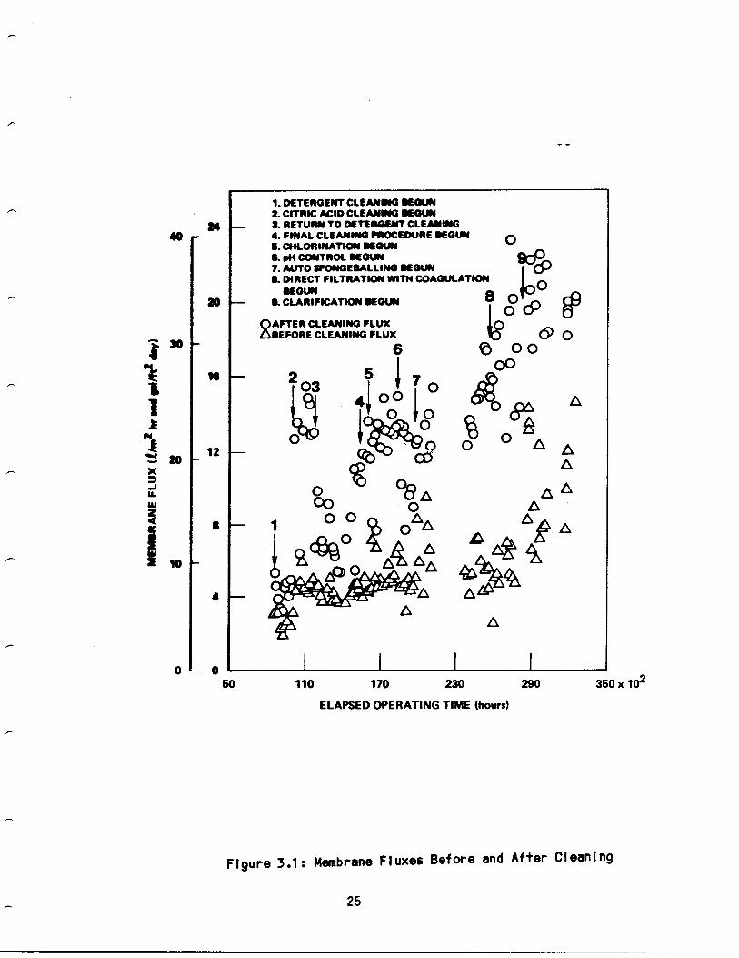
results of the improvements in cleaning techniques can be seen In Figure 3 .1

which shows the entire period of investigation for Phase I . The increases in

flux due to improved pretreatment are obvious . The increases in fluxes after

24

4

1

40

30

24

20

50

C9

RAFTER CLEANING FLUXBEFORE CLEANING FLUX

i

0 41

•

_A OAA%A. AA:

L I -"--Z#4

L

L~

I I

A

0

I

00

0

110

170

230

290

ELAPSED OPERATING TIME (hours)

Figure 3 .1 : Membrane Fluxes Before and After Cleaning

25

350 x 102

NE

1220

XJ

WztC

II 10

4

0 0

1. DETERGENT CLEANING MOM2. CITRIC ACID CLEANING BEGUN_. RETURN TO DETERGENT CLEANING4. FINAL CLEANING PROCEDURE BEGUN

OB. CHLORINATION BEGUNi. ON CONTROL BEGUN

Sop7. AUTO WWONGEBALLING BEGUNB. DIRECT FILTRATION WITH COAGULATIONWORN

O

8B CLARIFICATION BEGUN

O „n0011

January, 1978 were due to improved pretreatment techniques, rather than addi-

tional membrane cleaning techniques . This cleaning technique provides essen-

tially complete membrane cleaning and was not changed for the remainder of the

study .

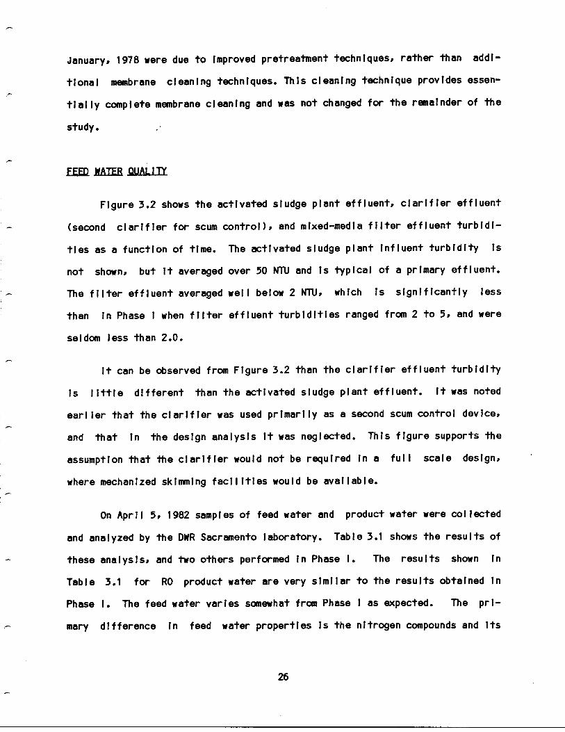
FAD WATER QUALITY

Figure 3 .2 shows the activated sludge plant effluent, clarifier effluent

(second clarifier for scum control), and mixed-media filter effluent turbidi-

ties as a function of time . The activated sludge plant influent turbidity is

not shown, but it averaged over 50 NTU and is typical of a primary effluent .

The filter effluent averaged well below 2 NTU, which is significantly less

than in Phase I when filter effluent turbidities ranged from 2 to 5, and were

seldom less than 2 .0 .

It can be observed from Figure 3 .2 than the clarifier effluent turbidity

is little different than the activated sludge plant effluent . It was noted

earlier that the clarifier was used primarily as a second scum control device,

and that in the design analysis it was neglected . This figure supports the

assumption that the clarifier would not be required in a full scale design,

where mechanized skimming facilities would be available .

On April 5, 1982 samples of feed water and product water were collected

and analyzed by the DWR Sacramento laboratory . Table 3 .1 shows the results of

these analysis, and two others performed in Phase i . The results shown in

Table 3 .1 for RO product water are very similar to the results obtained In

Phase I . The feed water varies somewhat from Phase I as expected . The pri-

mary difference in feed water properties is the nitrogen compounds and its

26

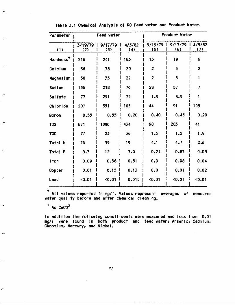
Table 3 .1 Chemical Analysis of RO Feed water and Product Water .

Parameter I

Feed water

{

Product Water

All values reported in mg/I . Values represent averages of measuredwater quality before and after chemical cleaning .

+ As CaC03

In addition the following constituents were measured and less than 0 .01mg/I were found in both product and feed water : Arsenic, Cadmium,Chromium, Mercury, and Nickel .

27

{(1)

3/19/79(2)

9/17/79 {(3)

4/5/82 13/19/79 9/17/79(6)

4/5/82(7)(4)

i (5)

Hardness + 216 241 163 13 19 6

Calcium 36 38 29 2 3 2

Magnesium 30 35 22 2 3 1

Sodium 136 218 70 28 57 7

Sulfate 77 251 75 1 .5 8.5 1

Chloride 207 351 105 44 91 105

Boron 0 .55 0 .55 { 0 .20 0 .40 0 .45 0 .20

TDS 671 1090 434 98 203 41

TOC 27 23 36 1 .5 1 .2 1 .9

Total N 26 39 19 4 .1 4.7 2.6

Total P 9 .3 12 7 .0 0 .21 0 .83 0 .05

Iron 0 .09 0.36 0 .51 0 .0 0 .08 0 .04

Copper 0 .01 0 .15 I 0 .13 0 .0 0 .01 0 .02

Lead <0 .01 <0 .01 I 0 .015 <0 .01 <0 .01 <0 .01I I I I

2

14.0

12.0

10.0

4.0

2.0

0.0

0.0

0

A

0 D O 00

00

Li

0O

0A

A

A 0 A

0 00

00

~m0

Li0

~0 Li

O

dNp 0 A

A

O

O

0

~O

r,0Q

99 E31% O olyIII11

20.0

40.0

60.0

80.0

100.0

DAY OF YEAR

28

0 ACTIVATED SLUDGE PLANT EFFLUENTA CLARIFIER EFFLUENT0 MIXED-MEDIA FILTER EFFLUENT

0

0

Figure 3 .2 : Turbldities as a Function of Time

forms . The nitrogen was almost 100% ammonia and organic nitrogen in Phase I,

while in Phase II the activated sludge plant provided partial nitrification,

reducing the ammonia concentration while increasing the nitrite and nitrate

concentrations . This difference is also reflected in the product water, since

with cellulose acetate membranes ammonia removal than nitrate and nitrite

removal . In Phase I the total nitrogen of the product water was in the range

of 4 to 7 mg-WI, while in Phase II it was less than 2 .0 mg-N/I .

FLUX DECLINE AM IHE EFFECTS DE PRETREATMENT

Improvements made in recovery and flux maintenance after January, 1978

were largely due to improvements in RO feed water quality . Chlorination of RO

feed water was begun in March, 1978, and feed water pH control (pH controlled

to approximately 5 .5) was begun in May, 1978. Both of these changes resulted

in small increases in flux maintenance . The pH control improved flux mainte-

nance due to the increased solubility of calcium sulfates and carbonates at

the reduced pH, while chlorination prevented the growth of fouling slimes on

the membranes . The actual purpose of pH control was to reduce membrane hydro-

lysis, but it also has this additional benefit .

The installation of the auto-sponge ball cleaning device in August,

1978, coincides with increases in before-cleaning fluxes to as high as 8 GSFD .

Unfortunately the high before-cleaning fluxes declined to the level of 5 to 7

GSFD during the period of October, 1978 to May, 1979 . No reason for this

decline was determined .

29

The use of chemical coagulation and clarification had very large effects

on both before and after-cleaning fluxes . Direct filtration with a cationic

polymer which was begun on May 31, 1979 coincides with increasing trends In

both before and after-cleaning fluxes . The before and after-cleaning fluxes

increased to maximum values of about 14 and 25 GSFD, respectively, during the

final periods of of Phase' I, when the inorganic coagulants were used .

Flux Decline Tests

During various times in Phase I and at the end of Phase II a series of

flux decline tests were made using various concentrations of ferric chloride,

alum, and organic coagulants . During the first phase the tests were conducted

over a twenty-four hour period, while in the second phase they were conducted

over a 48 hour period . Flux decline curves for representative tests from

Phase I are shown in Figure 3 .3, along with a tap water flux decline test,

which illustrates the flux decline caused by membrane compaction .

Unfortunately the flux decline tests performed in Phase II are not

directly comparable to those shown in Figure 3 .3, because of the differences

in membrane characteristics . It was noted previously that the membranes were

all replace beginning in July, 1981, due to deterioration during storage under

tap water pressurization. The new membranes were cast using the same pro-

cedure as previously and cured at 88°C as previously ; however the flux and

sodium rejection properties of the new membranes were different than the old

membranes . The new membranes were much "tighter" than the old membranes . The

old membranes removed TDS to an average level of 200 mg/I, while the new mem-

branes initially reduced the TDS to less than 50 mg/I and often less than 20

30

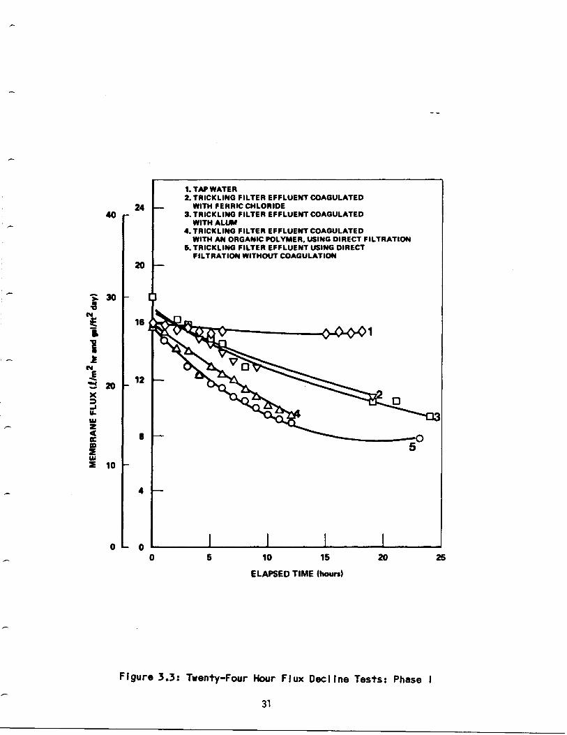
1. TAP WATER2. TRICKLING FILTER EFFLUENT COAGULATEDWITH FERRIC CHLORIDE

3. TRICKLING FILTER EFFLUENT COAGULATEDWITH ALUM

4. TRICKLING FILTER EFFLUENT COAGULATEDWITH AN ORGANIC POLYMER, USING DIRECT FILTRATION

5. TRICKLING FILTER EFFLUENT USING DIRECTFILTRATION WITHOUT COAGULATION

5 10

15

ELAPSED TIME (hours)

31

20

Figure 3 .3 : Twenty-Four Hour Flux Decline Tests : Phase I

25

mg/I . The after-cleaning flux of the old membranes averaged 15 to 20 GSFD,

and was sometimes as high as 25 GSFD, while the after-cleaning flux of the new

membranes was only 12 to 15 GSFD . This change in membrane properties is con-

sistent with an-increase in curing temperature, or may possibly be due to the

newness of the membranes . At the conclusion of Phase I, when most of the

twenty-four hour flux decline tests were performed, the membrane average age

was 1 .1 years, while the age of the membranes in the Phase II flux decline

tests was six months or less . No explanation of the difference in membrane

properties was determined .

In the design analysis performed later to determine the effects of pre-

treatment on design, a hypothetical condition was created which assumed the

existence of a membrane which had the same flux decline properties as the new

"tight" membranes, and the same salt rejection properties as the old mem-

branes . This was a conservative assumption because a "looser" membrane should

have higher fouling properties when biological materials are present (due to

the high flux and resulting high throughput of fouling materials) ; therefore,

flux decline should be higher with the old, "looser" membranes . The economic

analysis described later shows that the new, "tight" membranes provide a more

economical design ; therefore the question of why the new membranes were dif-

ferent and what there flux decline properties were, does not effect the final

conclusions of this study .

Figure 3 .4 shows the three flux decline tests performed in June, 1982

using filtered activated sludge plant effluent, alum coagulated, filtered

activated sludge plant effluent . and ferric chloride coagulated, filtered

activated sludge plant effluent .

32

0 0

1. ACTIVATED SLUDGE EFFLUENT USING DIRECTFILTRATION

2. ACTIVATED SLUDGE EFFLUENT COAGULATEDWITH FERRIC CHLORIDE

3. ACTIVATED SLUDGE EFFLUENT COAGULATEDWITH ALUM .

1

23

0 10

ELAPSED TIME (hours)

Figure 3 .4 : 48-Hour Flux Decline Tests-Phase II

3 3

20 30 40 50

2440

20

W 30

16

I

0tNE 12I 20

xJU.Wz4 8Irm2

a 10

4

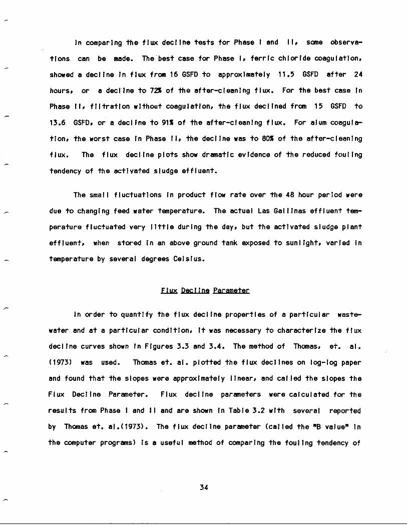
In comparing the flux decline tests for Phase I and II, some observa-

tions can be made . The'best case for Phase I, ferric chloride coagulation,

showed a decline in flux from 16 GSFD to approximately 11.5 GSFD after 24

hours, or a decline to 72% of the after-cleaning flux . For the best case in

Phase II, filtration without coagulation, the flux declined from 15 GSFD to

13 .6 GSFD, or a decline to 91% of the after-cleaning flux. For alum coagula-

tion, the worst case in Phase lip the decline was to 80% of the after-cleaning

flux . The flux decline plots show dramatic evidence of the reduced fouling

tendency of the activated sludge effluent .

The small fluctuations in product flow rate over the 48 hour period were

due to changing feed water temperature . The actual Las Gallinas effluent tem-

perature fluctuated very little during the day, but the activated sludge plant

effluent, when stored In an above ground tank exposed to sunlight, varied In

temperature by several degrees Celsius .

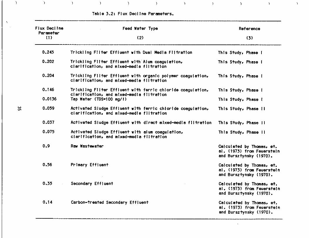
Flux Decline Parameter

In order to quantify the flux decline properties of a particular waste-

water and at a particular condition, It was necessary to characterize the flux

decline curves shown in Figures 3 .3 and 3 .4 . The method of Thomas, et . al .

(1973) was used . Thomas et . al . plotted the flux declines on log-log paper

and found that the slopes were approximately linear, and called the slopes the

Flux Decline Parameter . Flux decline parameters were calculated for the

results from Phase I and II and are shown in Table 3 .2 with several reported

by Thomas et . al .(1973) . The flux decline parameter (called the "B value" in

the computer programs) is a useful method of comparing the fouling tendency of

34

)

Table 3 .2 : Flux Decline Parameters .

Flux Decline

Feed Water TypeParameter

Reference

(1) (2) (3)

0.243 Trickling Filter Effluent with Dual Media Filtration This Study, Phase I

0 .202 Trickling Filter Effluent with Alum coagulation,clarification, and mixed-media filtration

This Study, Phase I

0 .204 Trickling Filter Effluent with organic polymer coagulation,clarification, and mixed-media filtration

This Study, Phase I

0 .146 Trickling Filter Effluent with ferric chloride coagulation,clarification, and mixed-media filtration

This Study, Phase I

0 .0136 Tap Water (TDS=100 mg/I) This Study, Phase I

W01 0 .059 Activated Sludge Effluent with ferric chloride coagulation,

clarification, and mixed-media filtrationThis Study, Phase II

0 .037 Activated Sludge Effluent with direct mixed-media filtration This Study, Phase II

0 .075 Activated Sludge Effluent with alum coagulation,clarification, and mixed-media filtration

This Study, Phase II

0 .9 Raw Wastewater Calculated by Thomas, et .al . (1973) from Feuersteinand Bursztynsky (1970) .

0 .56 Primary Effluent Calculated by Thomas, et .al . (1973) from Feuersteinand Bursztynsky (1970) .

0 .35 Secondary Effluent Calculated by Thomas, et .al . (1973) from Feuerstelnand Bursztynsky (1970) .

0 .14 Carbon-treated Secondary Effluent Calculated by Thomas, et .al . (1973) from Feuersteinand Bursztynsky (1970) .

a wastewater . The lower the flux decline parameter, the lower the fouling

tendency of the feed water. The small positive value of the flux decline

parameter for Marin tap water is probably due to membrane compaction . It is

obvious from Table 3 .2 than pretreatment significantly reduced the fouling

tendency of the feed water .

36

4. DESIGN ANALYSIS

The design approach used In this report draws heavily upon the technique

developed In Phase I . The Phase I technique was developed in part from previ-

ous work by Hatfield (1967), Hatfield and Graves (1970), Fan, et. al . (1970),

and McCutchan and Goel (1974) . The Phase I report (Davis, et . al . 1979))

should be consulted for a more complete discussion of the design and optimiza-

tion techniques .

FACILITY SIZE

Using the data collected in this study and the previous phase, the cost

data complied by the Oak Ridge National Laboratory (1980), and the EPA (1979),

an economic model was developed . When the model was developed in Phase i,

these two sources of cost data were current . Unfortunately these two sources

are still the most current cost data available . They have been updated

through the use of the Engineering. News-record, (ENR) cost updates to the

present in order to keep the financial calculations current . Table 4 .1 shows

the ENR Index, along with other indices frequently used .

The model is based upon using the RO product water In conjunction with a

specific quantity of RO feed water, to provide water for recycle with a speci-

fied water quality . The calculation procedure Is to determine the minimum

quantity of RO product water for blending with feed water to meet the speci-

fied water quality standards such as TDS, TOC, turbidity, and biochemical oxy-

gen demand . Pretreatment level and cleaning frequency are considered as vari-

ables, while RO operating pressure, membrane characteristics, and velocity are

considered constant .

37

Table 4 .1 : Cost Indices from Various Sources .

1 Engineering News-record index for the fourth quarter of each year .

e2 EPA national average index for 5 MGD plants for the fourth quarter ofich year.

CE plant cost index, published In Chemical Engineering4 M & S equipment cost index published in Chemical Engineering

38

Year

(1) ,

ENR1

ENR1

EPA2 CE Plant3Construction

Building(2)

(3)

(4)

(5)

M & S4

(6)

1978 1 2869

1734

145

218 545

1979 3140

1909

158

239 599

1980 3376

2017

169

261 660

1981 3705

2184

180

297 721

1982 3931 2294 746

BASIS fQ$,COST ESTIMATES

The least cost pretreatment system was found by simulating the RO unit

with various pretreatment alternatives . This basis of comparison for the

simulation was the flux decline parameter (B), for each pretreatment alterna-

tive, and the associated processes which provided the pretreatment . The flux

decline parameters shown previously Table 3 .2 were used in the simulation pro-

gram . The cleaning frequency was evaluated for each pretreatment alternative

and the value producing the least cost was found . The cost using this clean-

ing frequency for each alternative was then compared, and an optimal alterna-

tive was selected .

The costs for the pretreatment system processes were considered to be

log-linear functions using parameters calculated from the appropriate cost

reference. This is the technique of the EPA (1979) method . The assumption of

log-linearity corresponds well with the data for plants in the range of one to

ten MGD . The cost equations take the following form :

log 10 ( Cost Variable ) = a * log 10 ( Size Variable ) + b .(4 .1)

and

Cost = index * Cost Variable(4.2)

where

a and b are parameters from the EPA (1979) document,

and index is the appropriate cost update index shown in Table 4 .1 .

39

The functions were calculated for each of the five categories specified

in the EPA (1979) report which allows for variation of the costs for labor and

energy . Labor and energy costs are assumed independently of the EPA cost fig-

ures . For the analysis presented in the Phase I report, the cost of labor was

assumed to be $12.00/hr, while energy costs were assumed to be $0 .05/kWhr . It

was assumed for this report that these costs gradually increase to $16.84/hr

and $0 .07/kWhr . The interest rate was assumed to be 8% in the Phase I report

and has been Increased to 1296 for this analysis.

Implicit in this analysis are assumptions about scale up in technical

parameters such as fouling rate, and that costs per unit area for tubular and

spiral wound membrane modules will be similar . Brine disposal costs have not

been included, nor have any costs been assumed for the secondary treatment

system . Table 4 .2 summarizes the design and size variables, while Table 4 .3

shows the cost coefficients based upon the 1979 data. Sample calculations

using the technique describe herein were present in the Phase I report .

Table 4 .4 shows the optimal design for the 1 MGD hypothetical reclama-

tion plant using the new information generated in Phase II . Several differ-

ences should be noted . No coagulants are required, and in fact coagulants not

only add to the operating cost but reduce recoveries as well . This was not

true of the results of the Phase I . Energy consumption is less due to the

increased recovery rate and reduced number building and processes . Opera-

tional requirements are less since no coagulating chemicals are required . The

optimal results for Phase I are shown in the appendix . The results of all

alternatives, Including the four pretreatment alternatives evaluated in Phase

I, In terms of cost per thousand gallons, are presented in Table 4 .5 . Also

40

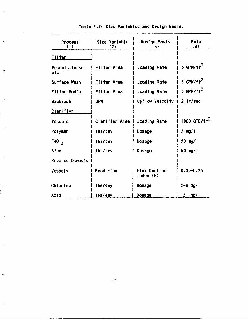
Table 4 .2 : Size Variables and Design Basis .

41

Process(1)

Size Variable(2)

Design Basis(3)

Rate(4)

F i I ter

Vessels,Tanks Filter Area Loading Rate 5 GPM/ft2etc

Surface Wash Filter Area IILoading Rate 15 GPM/ft2

IFilter Media

Backwash

Clarifier

Filter Area

GPM

I Loading Rate 15 GPM/ft2I

Upflow Velocity 1 2 ft/sec

Vessels Clarifier Area I Loading Rate 1000 GPD/ft2

Polymer lbs/dayIIIDosage 15 mg/I

IFeCI 3 lbs/day I Dosage 150 mg/I

Alum

Reveres Osmosis

Ibs/day Dosage 60 mg/I

Vessels Feed Flow Flux Decline 0 .05-0 .23

Chlorine lbs/dayII

Index (B)

Dosage 12-9 mg/It I

Acid I lbs/day I Dosage 115 mg/I

N

Table 4 .3 : Cost Coefficients for the Log-Linear Functions .

1 Value is approximately constant for the range ofconsidered values .

l

Cost Section

Total Capital (S) Energy(kWhr/yr) Operation and MaintenanceI Lights, Heating Process

I Materials ($/yr) Labor (hr/yr)4 Cooling i

a b a

b a b

I

a b a

b(1)

(2) (3) (4) (5) (6) (7)

I

(8) (9) (10)

(11)Filter I

Tanks & Vessels 0 .32 4 .72 21,000I

2 .47 0 .30

2.510 .97

2.47 1 0 .791 I

Surface Wash

0.24 3 .96 NA NA 0 .89 1 .45 10 .14 2 .00 0 .49

0.69

Filter Media

1 0.65 2 .55 NA NA NA NA I NA NA NA

NAI 1

Backwash

10.37 3 .49 NA NA 1 .00 1 .38 1 0 .28 2 .24 0 .062

2.15

ClarifieriI

Vessels

0 .32 4 .01 NA NA 0 .17 3 .02 0 .64 1 .57 0 .15

1 .74

Polymer 20,2001 8,2101 17,3001 2701 1981

FeC1 3

0.28 4 .00 0 .57 3 .20 4,9001 0 .067 2.19 0 .062 0 .067

Alum

I 0 .23 4 .08 0 .57 3 .22 4,9001 2001 0 .62

3.97I

Reverse Osmosis II

5 .89 0 .90 5 .02 0 .96

6.38 0 .19 3 .27 0 .89

4.99System ~ 0 .85

Acid i 0 .12 3 .82 3,680 1 1,6301 1 0 .33 1 .53 0 .22

1 .56

Chlorine 1 0 .36 3 .75 0 .52 3 .45 0 .17

2.58 ` 0 .11 2 .53 0 .18

2.57

Cleaning 1 0 .28 3 .31 NA NA 1 .0

1 .08 i 0 .62 2 .13 0 .28

2.16

3 . 14 2. 16 2 .03

Table 4 .4 : Optimal Design for a 1 MCD Facility . (3 pages)

THE L:MITING PARAMETER IS TDS FOR 13(8)= 0 .037

THE FOLLOWING WATER. QUALITY RESULTSFILTER RO REQUIRED BLENDED

TDS 1203. 250 .0 530 .0 500 .0TOC 18 . 1.0 15.0 5.5NTU 3. 0.5 2.0 1.2TSS

4.

0.0

5.0

1 .1

THE PA 'IO CF BLENDED FO P^ODUCT WATER TO TOTAL PRODUCT FLOW = 0 .737

ASSUMPTIONSLABOR RATE = $ 16.84 PER HOUR

ELFCTPICAL PATE = $ 0 .07 PER KWR

INTEREST FATE =

12.00%

LI7F OF PROJECT =

20 YEARS

INFLATION RATIO =

1.370

PrOJ•CT YEAR =

1983

COSTS PER KGALS FOP VARYING VALUES OF B AND '"HE CLEANING INTErVAL

CLEANING INTERVAL (HOURS).1

8

16

24

32

40

48

56

64

72

80

' . 0^

1.98 1 . 9F

1.Q8 1 .98

1 .98

1 .99 1.99

43

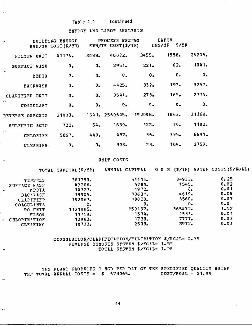
Table 4 .4

Continued

ENERGY AND LABOR ANALYSIS

UNIT COSTS

COAGULATIO N/CLAEIFICATION/FIL'RATION $/KGAL= 0 .39REVERSE OSMOSIS SYSTEM $/KGAL= 1 .59

TOTAL SYSTEM $/KGAL= 1 .98

THE PLANT PRODUCES 1 MGD PER DAY OF THE SPECIFIED QUALITY WATERTHE TOTAL ANNUAL COSTS = $ 673065 .

COST/KGAL = $1 .98

44

BUILDING ENERGYKWH/YR COST ($/YR)

PROCESS ENERGY LABORARS/YR $/YRKWH/YR COST ($/YR)

FILTER UNIT 41176 . 3088. 46072 . 3455 . 1556. 26205 .

SURFACE WASH 0 . 0. 2951 . 221 . 62 . 1041 .

MEDIA 0 . 0. 0 . 0 . 0 . 0.

BACKWASH 0 . 0. 4425. 332 . 193 . 3257 .

CLARIFIER UNIT 0 . 0 . 3641 . 273 . 165 . 2776 .

COAGULANT 0 . 0 . 0. 0 . 0 . 0.

REVERSE OSMCSIS 21893 . 1641 . 2560645 . 192048 . 1863 . 31368 .

SULFURIC ACID 722 . 54 . 1630. 122 . 70 . 1182 .

CHLORINE 5867 . 440 . 487 . 36 . 395. 6644 .

CLEANING 0 . 0 . 308 . 23 . 164 . 2759 .

TOTAL CAPITAL (S/YB) ANNUAL CAPITAL 0 E M ($/YR) WATER COSTS ($/KGAL)

VESSELS 381790. 51114. 34933. 0 .25SURFACE WASH 43206. 5784 . 1545 . 0 .02

MEDIA 14727. 1972. 0 . 0 .01BACKWASH 79405. 10631 . 4619 . 0 .04

CLARIFIEP 142067. 19020. 3560 . 0 .07COAGULANTS 0. 0 . 0. 0 .0

PO UNIT 1121885. 150197. 365472. 1 .52H2SO4 11759. 1574. 1531 . 0 .01

CHLORINATION 12983. 1738. 7777. 0 .03CLEANING 18733. 2508. 8972. 0 .03

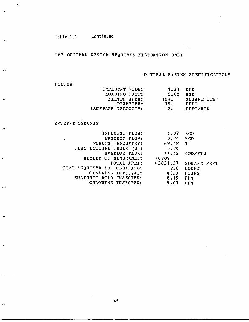
Table 4 .4

Continued

THE OPTIMAL DESIGN REQUIRES FILTRATION ONLY

OPTIMAL SYSTEM SPECIFICATIONS

45

FILTERINFLUENT FLOW : 1 .33 N:GDLOADING RATE : 5 .00 MGDFILTER AREA : 184 . SQUARE FEET

DIAMETER : 15 . F•FTBACKWASH VELOCITY : 2 . FFET/MIN

REVERSE OSMOSIS

INFLUENT FLOW : 1 .07 MGDPRODUCT FLOW : 0 .74 MGD

PERCENT RECOVERY : 69 .18FLUX DECLINE INDEX (B) 0 .04

AVERAGE FLUX : 17 .12 GPD/FT2NUML3EF OF MEMBRANES : 18709

TOTAL APEA : 43031 .37 SQUARE FEETTIME ELQUIEED FO:: CLEANING : 2 .0 HOURS

CLEANING INTERVAL : 40 .0 HOURSSULFURIC ACID INJECTED : 8 .19 PPM

CHLORINE INJECTED : 9 .00 PPM

Table 4 .5 : Treatment Cost in Dollars per Thousand Gallons for a 1 MGDReverse Osmosis Wastewater Reclamation Facility .

*CODES

TYPE OF PROCESS AND PRETREATMENT*

FOR PROCESS AND PRETREATMENT

TF = Trickling Filter Secondary Treatment

ASP = Activated Sludge Process Secondary Treatment

FeCI : Coagulation, Sedimentation, and FiltrationusiWferric chloride as a coagulant .

Alum : Coagulation, Sedimentation, and Filtrationusing alum as a coagulant .

Nalco : Coagulation, Sedimentation, and Filtration usingNalco cationic polymer as a coagulant .

None : Filtration with no coagulation or sedimentation .

+ Hypothetical membrane having the same fouling propertiesas the tight membranes used in the second phase, but having fluxand TDS removal properties similar to the membranes used in thefirst phase .

4 6

Year I TFj FeCl 3 1I TFNalco

I TF` Alum

I TF` None I

I ASPI Fedl 3I ASP` None

I' ASPi Alum

I ASP'I None

1979

1 .57

1 .81

2.09

1 .70

1 .22

1 .11

1 .65

1 .29

1980

1 .84

2.11

2.41

1 .99

1 .42

1 .30

1 .89

1 .50

1981

2.04

2.33

2.67

2.21

1 .58

1 .45

2.09

1 .67

1982

2.22

2.53

2.91

2.40

1 .72

1 .57

2.29

1 .82

1983

2.42

2.74

3.17

2.61

1 .87

1 .71

2.49

1 .98

Included in Table 4 .5 is the hypothetical membrane, described earlier, which

was used to evaluate the potential effects of the "tight" membranes used in

the Phase II . It is observed that this membrane did not provide the least cost

alternative. The cost values are considered tentative due to the ambiguities

of scale-up .

47

5. CONCLUSIONS

The results of an experimental and theoretical analysis of a 10 GPM

pilot plant for producing reclaimed water has been presented . The results

were applied to the design of a full scale 1 I4GD facility . In addition to the

conclusions presented in the Phase I report (none were contradicted in this

phase of research), the following additional conclusions are made :

1 . The activated sludge plant effluent had significantly less tendency

to foul the membranes than trickling filter effluent, indicating

that a major source of fouling material in Phase I was organic

material . This corroborates the predictions from the fouling

material analyses performed In Phase i . The activated sludge plant

followed by direct filtration produced feed water which had only

one-third the fouling tendencies of the best trickling filter

effluent which could be obtained from the Las Gallinas facilities .

2 . Cleaning using flushes of citric acid, followed by enzyme detergent

and sponge ball cleaning were effective at maintaining membrane

flux to essentially the initial flux levels . The citric acid was

the major cleaning agent. Enzyme detergent and/or sponge ball

cleaning without citric acid were relatively ineffective .

3 . The automatic sponge ball cleaning technique appeared to have prom-

ise for maintaining membrane flux between chemical cleanings .

Further testing is desirable .

4 .

The major factor contributing to membrane degradation for the type

of membranes used In this study was corrosion of the end couplings .

48

The average membrane life during Phase I was 10 .000 hours .

5 .

The chance production of tighter membranes reduced the total

operating cost by $0 .27 /1000 gallons .

6 .

The greatest level of pretreatment again produced the least cost

alternative .

7 . Alum was always the poorest coagulant, which was probably due to

carry over into the RO unit of aluminum hydroxide which has minimum

solubility at pH=5 .5 .

49

REFERENCES

1 . Anderson, D . R. and Mills, W. R ., (1977) "An Integrated Pretreat-ment System for High Recovery Reverse Osmosis Systems," Desalina-tion, Vol 22, pp 349-357 .

2 . Antoniuk, D . and McCutchan, J. W . (1973) "Desalting IrrigationField Drainage Water by Reverse Osmosis, Firebaugh, California,"UCLA-SEAS Report, UCLA-ENG-7368 .

3 . Argo, D . and Moutes, J . G., (1979) "Wastewater Reclamation byReverse Osmosis," Journal Q{ 1bg Water Pollution Control Federa-tion, Vol 51, pp 590-600 .

4 . Asano, T., Ghirelli, R., and Wasserman, K . L ., (1979), discussionof "Wastewater Reuse by Biological-Chemical Treatment and Ground-water Recharge," by Idelovitch, E ., in Journal j j Water Pollu-tion Control Federation, Vol 51, pp 2327-2329 .

5 . Davis, J . R ., Stenstrom, M. K. and McCutchan, J . W., (1980)"Improvement of Reverse Osmosis Through Pretreatment," UCLA-SEASReport No . UCLA-ENG-80-66, School of Engineering and Applied Sci-ence, University of California, Los Angeles, California .

6 . Department of Water Resources (1983), "Agricultural Waste WaterDesalination by Reverse Osmosis, Final Report, Phase II," Bulletin196-93, May, 1983, Sacramento, California .

7 . Environmental Protection Agency, (1979) "Estimating Water TreatingCosts," US EPA Publication EPA-600/2/-79/162a through 162/b, Vol1-4 .

8 . Feuerstein, D.L ., and Bursztynsky, T.A., (1970) "Design Con-sideration for Treatment of Solids-Laden Wastewaters by ReverseOsmosis," AIChE Water, Y_Qj °Z, a 5„A-5a.

9 . Goel, V. and McCutchan, J . W ., (1978), "Systems Design of a Tubu-lar Reverse Osmosis Plant," UCLA Engineering Report, UCLA-ENG-79-04 .

10 . Hatfield, G. (1967), "Digital Computer Simulation and Optimizationof a REverse Osmosis System," MS Thesis, School of Engineering andApplied Science, University of California, Los Angeles, LosAngeles, CA .

11 . Hatfield, G . and Graves, G. (1970) "Optimization of a ReverseOsmosis System Using Non-Linear Programming," Desalination, Vol 7,pp 147-177 .

12 . Johnson, J . S. and Loeb, S . (1966), "Reverse Osmosis Desalinationat the Coalinga Plant : Progress Report January 1, 1966 to June 1,1966," Water Resources Center Desalination Report No .

7 .

50

University of California, Davis, California .

13 . Johnson, J . S. McCutchan, J . W. and Bennion, D . N ., (1969) "Threeand One-Half Years Experience with Reverse Osmosis at Coalinga,California," UCLA-SEAS Report No . UCLA-ENG 69-45, School ofEngineering and Applied Science, University of Ca-fifornia, LosAngeles, California .

14 . Loeb, S., and SouriraJan, S . (1960) "Sea Water Demineralization byMeans of a Semi-permeable Membrane," UCLA-SEAS Report No . UCLA-ENG-60-60 .

15 . Loeb, S., and SouriraJan, S ., (1962) "Sea Water Demineralizationby Means of an Osmotic Membrane," AU, Saline Water Conversion-l,pp 117-132 .

16 .

Metcalf and Eddy, (1979) Wastewater .Engineering Treatment, Dispo-cal And Reuse second edition, McGraw-Hill, New York, NY .

17 . Office of Saline Water and Bureau of Reclamation, (1972), Desalt--Loa Handbook IQC planners, U.S . Department of the Interior, Wash-ington, DC, May, 1972

18.

Reynolds, T. D ., (1982), Unit Operations jLpd, Processes JA Environ-inental Engineering, Wadsworth,Inc, Belmont, California .

19 . Speight, L . W . and McCutchan, J. W., (1979) "Reverse OsmosisDesalination Plant Design and System Optimization Based on theFacility at Firebaugh, California," UCLA-SEAS Report No . UCLA-ENG-7982, School of Engineering and Applied Science, University ofCalifornia, Los Angeles, California .

20 . Stenstrom, M.K., Davis, J .R ., Lopez, J . and J .W . McCutchan, J .W .,(1982), "Municipal Wastewater Reclamation by Reverse Osmosis : AThree-Year Case Study," Journal .Qf ƒ Water Pollution ControlFederation, Vol 54, pp 43-51 .

21 . Thomas, D .G., Gallaher, R .B ., and Johnson, J .S ., (1973), "Hydro-dynamic Flux Control for Wastewater Application of HyperfiltrationSystems," US EPA report EPA-R2-73-228 .

22 .

Torpey, W.N., (1948),

"Practical Results of Step Aeration,"Sewage Works Journal, Vol 20, pp 781-787 .

23 . Zachariah, M. R., (1982) "Analysis of Reverse Osmosis MembraneDegradation by Instrumental Techniques," MS Thesis, School ofEngineering and Applied Science, University of California, LosAngeles, 1982 .

51

APPENDICES

52

ES

(Z8-t86L) KINHOdITYO SSYRIZY9 Sri - Y.LVQ XQ'I3 xiIYa

Z8/0•/9 0; Z8/UL wojj kaeuwns e;ea „ L x Lpuaddy

9MINV D TIYHa9NOdS QNV THDIW390 - *9NINY3T0 TTBSa9NO3S - +

L00'L LL - EL ZS'E 'ZLL '0 'COLL Z8/E0/90+LSL'O EE '0L 617 1 E '69 *OOZE '008 Z8/E0/90OE8'0 8S 'LL LSE 'ZOL 'OOOS 'OSL E8/E0/90L00'L L9 'EL ES'E '08L '0 "0S8 z8/LO/90*LLS'0 6L'L S17'E 'SS '0S6L 'SL 8 ZB/LO/90LE8'O LZ'L L Ltt'E '88 'OOOS "006 ZB/8Z/SOE06'3 06 'LL LE'E '06L 'OOtt8 'OSLL Z8/LZ/(-.-0+6L9'0 LS '8 tiS'E 'ZL '009L '00LL Z8/LZ/S0LL6 - 0 89'ZL 9S'E '8ZL 'OSZZ *008 Z8/SZ/SOS99'0 6E'6 L 9 1E '88 'OOZZ 'SZ8 Z8/SZ/SOL86'0 S8'EL 65 1 E 'S SL '0082 'SLL ZS/trz/SU*ZZ9'0 69'9 LS'E 'Ztr 'OOOZ 'SZL ZB/t7Z/S0EEL'0 6h'Ot 99 1 E '0 ti 'OOLZ '0S9 ZS/LZ/SOZL6'0 08'ZL 6S'E '8L 'SLS ZB/0Z/S0+1799 -0 : Ltt'6 ttsIE 'SE '006L 'SLS z8/OZ/SOLEL'O Lb'OL L9`E '88 '00EL '009 ZB/6t/50LLL"O 9L'0L ttS'E 'L9L 'OOOZ '009 z8/8L /soL86'0 L8 'El 9S'E '08 1 000E 'OSS ZS/LL/SO*6617'0 SS'9 LS'E 'ZS 'S01L 'SLS Z8/LL /SOEZ9'0 ES'8 OS'C 'SE '006 '009 za/ttt/soZG8'0 EZ'LL BS'E '99 'OOLZ 'SZ9 ZB/EL /S0+ZLL'O 176'6 LS'E '1717 '00EZ 'CS9 Z8/ZL/SO9EL'0 Wet OL'E 'SIZ '096 '059 ZB/LL/SO6E6'0 66'ZL 175 1 E 'Z6 'OOOZ 'OS9 Z8/OL/S0*1755'0 L9'L ti SIt 'SE ISZttL 'SZ9 ZB/0L /SO096'0 L6 'EL ZL'E '0L 'OOSZ 'OS9 ZS/90/SO+S9L'O LL 'Ot Ott'E 'S8 '00017 '0S9 Z8/90/so6E8'0 6E "LL Lti It 'Z8 '00Ltr 'OS9 z8/so/soSSL'0 OL'EL 179'17 "Z0Z '0S9 'SZ9 Z8/170/SOZS6'0 L0'EL L S'E 'SOL '009L 'OS9 Z8/E0/SO*L09'O LE'8 ES'E 1 9E 1 0091 1 099 Z8/co/S0E06'0 C9'ZL LSE '99 '006Z 'OOL Z9/6Z/t101i06 - 0 titt'Zt ZS'E '1717 'OOZ.Z 'SL9 Z8/6Z/170+999'0 SE'6 6S'E 'OS 'OOOZ 'OOL ZB/6Z/170EE9'0 8O'6 L9'E '091 '0S6 'SL9 ZB/8Z /170171L "0 CS 'OL L9'E '8EZ '00t1 'OS9 Z8/a/170

xS3A0038 USE)) Xn'I3-- ZOQQOHd

(HaO) MUZ3 ZOnoosa at:ISS QS33Q33d

SQ,L

Sad

SQb21YQ

ti5

DHINY213 TTY8afN0dS QKY TYJIh3HJ -

(ZS-L 861) YIt:&U3I'IYJ ' St NITY9 SYT - YZYQ Xo'r, i'IIYQ

panULIU00 l xLpuaddy

9NINY3T, TTY839N03S - +

9E6'0 L0 „• L LS'C '06 'OOSZL C59 Z8/9Z/fro*fiZ9'0 L9 . 8 E S'E '8E „0S61 '008 ZB /93/1,0LS8'0 Ot „Z L OL'E Z L 'OOSfi '009 ZB/EZ/tt06L6 . 0 Z9 „E l 6 L'E 'ZO1 '0SZOL 'SLS za/zz/1,o+508'0 LI'LL •S „E 'Z9 „0581, 'OSS Z8/ZZ/1,0OEL'0 EE lot Z 9 1 C '8fiZ 'OS6 '06S za/LZ/1,o606'0 LE'Z l 81,' E '8L 'OOL9 1 055 za/oz/1,o956 . 0 tic IT L LS'E Z 1, „0 StiZ '055 Z8/6L/1,0*1,09'0 St . 8 8S'E , SS losct loss Z8/6L /1,0009 . 0 611'8 Z 9 „E 'OL „0 0ZL 'OOS Z8/6L/1,0•06'0 LZ „L L 6S'E 'Z9 '009 'SZS Za/9l /1,09E8'0 06' L L 1,9'• 'L9 „O 5LL '009 Z8/SL/1,0+06S'0 ED - L 6•'E 'S8 'OOL1, 0 0LL Z8/SL /1,0808'0 SL *LL E S'E 'OL 'OSZZ 1 058 Z8/fil/1,09L9'0 •1,'6 LSE 'Z1, „0 501 0 517 ZB/fit /1,00ZL'0 1,6'6 ES 'E '50Z 'OCEL 'S8E ze/EL/1,oZL6'0 08 „Z L 6S'E '0S „0 0LL loot ZB/ZL /1,0*969 . 0 80'6 trS'E '6E ' CSL L - 009 z8/oL/1,oOL6'0 1,E „E L 5L'E '89 '00EL 1 009 Z8 /60/1,0+1,65'0 ES „8 L9'E It, 17

1 00•1 '009 28/60/1,0E6L'O SE It L 99 1 E 'SL „O SZL - 009 38/80/1,01168'0 tie lot 0L 'E L 1, `00LL 0 09 ZB/L0/1,08L8 . 0 1,L' L L L9'E 1 09 1 0092 . 061, ZB/SO/1,0*L9tr'0 S9'9 69 1 E 'OZ 'SL8 '0111, za/so/1,oLS9'0 OZ '6 8 S' E 'tr Z

"00Z L 'oz tr Z8/Z0/1,U6•9'0 ZL'6 S9'E '06

„S Etr 109E ZB/Z0/1,0169'0 OL'6 65 1 E 8 E '008 O Z1, Z8/L0/1,0+t709 '0 S5 'L OZ „E 5 1, '00LL lost ZB/LO/1,0ZL9 . 0 LL 'L zZ „E 'ZEL „O SL loss Z8/LE/EO17t79 -0 EE '8 L E'E 'SLZ '008 0 09 za/oE/EoS06'0 LULL tit - [ 'ZOL '00LL 'OOL Z3/6Z/co*8E1,'0 S9 . 8 So „S 8 Z „SZZL '00L Z8/6Z/E0617S'O 1,8 . 0L so's '00L Za/9Z/EO'OZL „O OZLZ09'0 L0'zL OL'S '059 ZB/SZ/E0+'Zfi '05518LS'0 1,L „6 L8'1, '1,Z '00EL '059 ZB/SZ/EOEES'0 ZO'OL L 8'11 '8L '0081 '059 ZB/1,Z/EOSZ9'0 t1L'll OE3'1, '91,

„OSLL 1 539 Z8/EZ/EO1S9'0 6Z 'Z L ES „1, '00L '0061 . 0CL Z8/ZZ/EO*6L1,'0 80 - 6 S„8 't S ZZ „0 5S• 'OSSL ze/zz/EoELS „0 98 . 6 26 . 1, - 68z 1 0005 '000? Z8/6t/[O

assnoo3s (as!)) xnT3 (as!)) mow sonao3d 3NZ2ig a33a 3ZYQ--ionaOid a a a a SCW

sas s c,L

SS

(Z8-t66L)YINHOaI'IY3 'SYNI .Y9 SYZ - YLYQ Xn'I3 f1YQ

panu 3uo0

„ 1 x!puaddy

9NINYa'J 'IIYSSONOdS UNY ZY3IWZR3 -DNINYaID i7vea9NOIS - 4

L6S'0 SELL L6 - ft 'EE 'OOtt loss Wet /Eo+E917 0 h8 '8 Be It '6L 'OSOL '06h Wet /cctr9h'0 h6 '8 LB 'h 'OZ 'OOLZ '0S9 Z8/LL/E068S'0 EZ'LL 88'h '.Sh '000Z 'OOL ZB/SL/EO*LLt'O OZ'6 66'h 'SE 'C08L 'SLL Z8/SL/E0OLL'0 ZS'ZL 9L'tr 'Z9 '000Z '0S8 ZB/OL/EU+07t '0 L9'8 Z6'h 'Z• 'OOLZ 'SZL ZB/OL/EOO•9'0 98'LL L8'h 'htr 'OOOZ 'OOL Za/RO/EO*ZOS'O 6S'6 88't 'OZ 'OOht 'OOL ZB/80/E0109'0 6L 'L L 9L - ft 'SE '008L ' SL9 ze/SO/E0+LSh'0 00'6 tic's 'hZ '0S91 'SL9 ZB/SO/EO6P1'0 •S'8 86'h 'SZ '009L 'SZ9 ze/EO/EoZZS'D 06'6 S8 'h '6Z '0S8 'SL9 Z8/ZO/E08L9'0 E6'LL h6'h 'hE 'OS•L 'SZL Z8/LO/EO*LSh'0 88'8 h0'S 'LZ 'OSEL 'SZL Z8/LO/E0665'O 98 'LL 90'S '0S 'SZ81 'SZL Z8/9Z/Z0+e6h'0 Z8'6 h0 'S '8Z 'OOSL 'SZL Z8/9Z/ZOOS9'0 L6'EL OS'S - Lt '0S8L 'COL ZB/ZZ/ZO*6Sh'0 Z6'8 L6 'h '•Z 'SZEI '00L Z3/ZZ/ZOZ9S'0 L9'6 Oh 't 'LZ 'SL9L '0S9 ZB/6L/ZO189'0 L6'EL sz -S 'Lt 'OOLL 'OSS Z8/Lt/ZO*h8h'0 •h '6 86'tt '6Z 'OSt L 'SZL ZB/LL/ZOSh5'0 EE'OL S8'h 'OE 'SLOL 'SLS ZB/9t /ZO+h9tt'0 LL'8 E8 'h 'SL '0S6 loos Z8/9L /Z0hSa'0 6tt'8 8L'h 'hE '008L 'US8 ZB/LL/Z0+98E'0 Zt'L ZL'h 'EZ 'OOSL '006 Z8/LL/Z09Ztt'0 6L'L 89'h It Z '009L '0S8 ZB/OL /ZOh9h'0 L9'8 SL'h 'hE - C06L - 006 ZB/80/ZOZ9S'O 8L '8 ZL'E 'Sh 'OSLZ '006 Z6/RO/ZOP99 10 L9'6 OL'E 'EE 'OSSZ 'SZ8 ZB/90/Zo6R9'0 ZO'OL ZL'• 'Z9 'OSEZ 'SLL ZB/SO/Zo60h'0 ZO'OL 9Z'9 '6L 'OSZL 'OSL Z8/h0/ZO69tt -0 BS' L L L 1o9 '6h 'OShL 'OOL Z3/ZO/Z0+L9E'O 69'8 90'9 'SL 'SZOL 'SLS Z8/ZO/ZOMOO EL'8 hl'9 '9L '000L 'OS9 ZU/LZ/LOZ8E'0 9L'6 EL'9 '6Z 'OSttL 'OOL Z8/8Z/t06L•'O LZ6 SZ - 9 '9Z -ocot loss ZB/SZ/LOZCtt'0 CO'6 EL'S 'OZ 'SLL '009 ZB/SZ/LU8Lh'0 Z8'6 SZ'S '9Z lost L '009 z8/CZ/L0Z6h'0 OL'OL SZ'S '0t 'OS6 'OLS ZB/ZZ/LO

x2i3Ao3 a (3S9) xn a--LDnaoaa

(i~dD) ro'I I imac`?d HNIL$ asa331

Sal

SQ,L

SQ,L31YQ

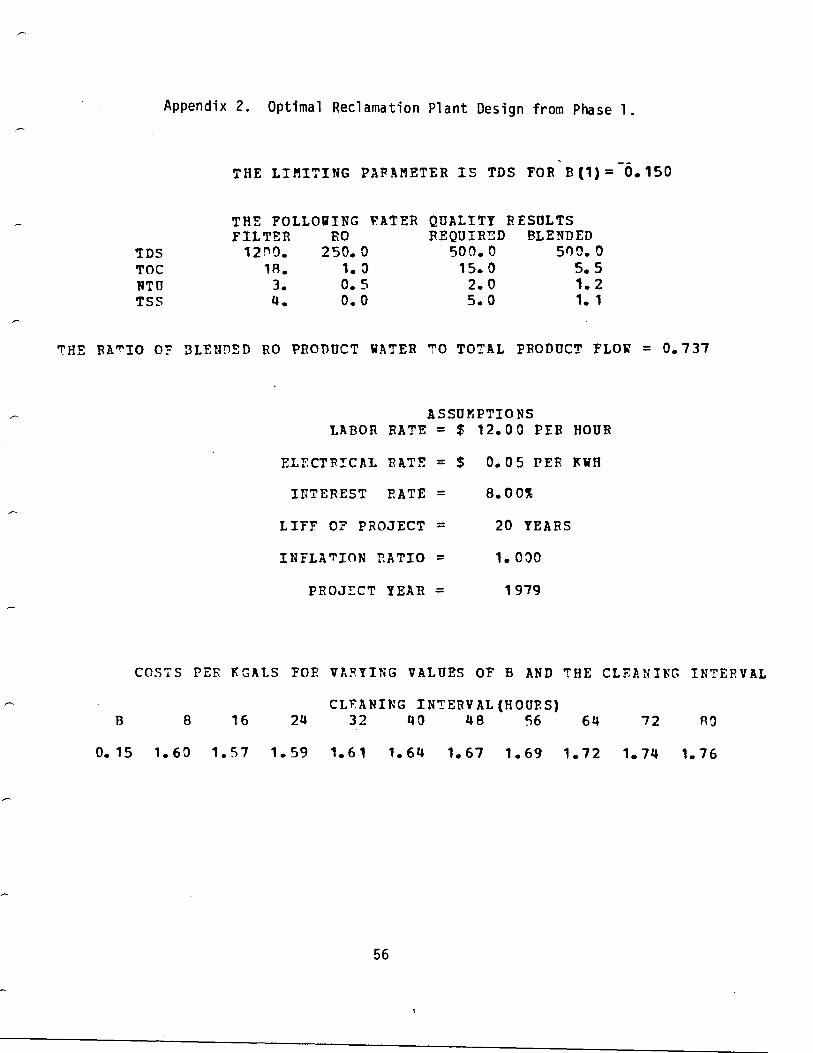
Appendix 2 . Optimal Reclamation Plant Design from Phase 1 .

THE LIMITING PARAMETER IS TDS FOR B(1)= 0 .150

THE FOLLOWING EATER QUALITY RESULTSFILTER RO REQUIRED BLENDED

TDS 12^0. 250.0 500.0 500.0TOC 1R. 1.3 15.0 5.5NTU

3.

0.5

2.0

1.2TSS

4.

0.0

5.0

1.1

THE RATIO OF BLENDED PO PRODUCT WATER TO TOTAL PRODUCT FLOW = 0 .737

ASSUMPTIONSLABOR RATE = $ 12.00 PER HOUR

ELECTRICAL RATE = $ 0 .05 PER RWH

INTEREST RATE =

8.00%

LIFT OF PROJECT =

20 YEARS

INFLATION PATIO =

1 .030

PROJECT YEAR =

1979

COSTS PER GALS FOR VARYING VALUES OF B AND THE CLEANING INTERVAL

CLEANING INTERVAL (HOURS)B

8

16

24

32

40

48

56

64

72

n3

0. 15 1 .60 1 .57 1 .59 1 .61

1 .64 1.67 1 .69 1 .72

1.74

1.76

56

Appendix 2 .

Continued

THE CPTIMAL DESIGN CONSISTS OF A CLARIFICATION/FILTRATION PRETREATMENTWITH FEERIC CHLORIDE ADDED AT 50 . PPM

OPTIMAL SYSTEM SPECIFICATIONS

F_LTER

57

INFLUENT FLOW :LOADING PATE:FILTER AREA :

1 .835 .00

253 .18 .2 .

1 .831010 .001822 .

48 .16

MGDMGDSQUARE FEETFEETFEET/MIN

DIAMETER :BACKWASH VELOCITY :

CLARIFIERINFLUENT FLOW :LOADING RATE :

CLARIFIER AREA :

MGDMGDSQUAF,EFEET

FEETDIAMETER :

COAGULANT : FERRIC CHLORIDE

REVERSE OSMOSIS

INFLUENT FLOW : 1 .56 MGDrRODUCT FLOW : 0 .74 MGD

PTFCEN _̂ RECOVERY : 47 .31 XFLUX DECLINE INDEX (R) 0 .15

AV EFAGE FLUX : 11 .71 GPD/FT2NU3BE7 OF MEMBRANES : 27359

TOTAL AREA : 62927 .18 SQUARE FEETTIME REQUIRED FOR CLEANING : 2.0 HOURS

CLEANING INTERVAL : 16 .0 HOURSSULFURIC ACID INJECTED : 8 .19 PPM

CHLORINE INJECTED: 2 .00 PPM

Appendix 2 .

Continued

ENERGY AND LABOR ANALYSIS

UNIT COSTS

COAGULATION/CLARIFICATTON/FILTRATION $/KGAL= 0 .28REVERSE OSMOSIS SYSTEM $/KGAL= 1 .29

TOTAL SYSTEM $/KGAL= 1 .57

THE PLAN PEODt1CES 1 MGT) PFF DAY OF THE SPFCIFIED QUALITY WATERTHE TOTAL ANNUAL COSTS = $ 533288 .

COST/KGAL = $1 .57

58

BUILDING ENERGYKWH/YR COST($/YF)

PROCESS ENERGY LABORHRS/YR S/YP-KWH/YR COST($/YR)

FILTER UNIT 41176 . 2059. 62520 . 3126 . 1711 . 20533 .

SURFACE WASH 0 . 0 . 3904 . 195. 72 . 865.

MEDIA 0 . 0 . 0 . 0 . 0 . 0 .

BACKWASH 0 . 0 . 6066 . 303 . 197 . 2367 .

-- CLARIFIER UNIT 0 . 0 . 3844 . 192 . 173 . 2076 .

COAGULANT 2262 . 113 . 4900. 245 . 308 . 3701 .

REVERSE OSMOSIS 30819 . 1541 . 3690893 . 184545 . 2001 . 24008 .

SULFURIC ACID 722 . 36. 1630 . 82 . 80 . 955.

CHLORINE 3175 . 159 . 396 . 20 . 348 . 4171 .

CLEANING 0 . 0. 658 . 33 . 172 . 2061 .

TOTAL CIPITAL(S/YP) ANNUAL CAPITAL

0 & "1 ($/Yr) WATER COSTS($/KGAL

VESSELS 308269 . 31398. 26706 . 0 .17SURFACE WASH 34017 . 3465. 1214. 0 .01

MEDIA 13204. 1345. 0 . 0 .00BACKWASH 65133 . 6634 . 3425 . 0 .03

CLAR:FIER 114782 . 11691 . 2662 . 0 .04COAGULANTS 26155 . 2664 . 4228. 0 .02

FO UNIT 11302Q7. 115124 . 318825 . 1 .24H2SO4 8979. 915. 1185. 0 .01

CHLORINATION 6162 . 628. 4684 . 0 .02CLEANING 23102 . 2353. 6178 . 0 .03

CCCCCCCCCCCCCCCCCCCCCCCCCCCCCCCCC PTOCFSSCCCCCCCCCCCCC

Appendix 3 . Computer Model Program Listing .

MAINTHIS PROGRAM IS DESIGNED TO GIVE THE OPTIMAL CONFIGURATION

FOR A REVERSE OSMOSIS SYSTEM GIVEN THE ALTERNATIVES OF DIRECTFILTRATION OR COAGULATION/FILTRATION WITH VARIOUS COAGULANT AIDS .VARIOUS VALUES OF THE FLUX DECLINE INDEX (B) WHICH CORRESPOND WITHDIFFERING LEVELS OF TREATMENT-(DIRECT FILTRATION AND--COAGULATION/FILTRATION WITH DIFFERENT COAGULANTS) HAVE BEEN DETERMINED FROMFIVE YEARS OF OPERATING AT LAS GALINAS, CALIFORNIA. THESE ARETESTED ALONG WITH DIFFERING CLEANING FREQUENCIES TO DETERMINE THELEAST COST ALTERNATIVE .

SUBROUTINESBLEND

CALCULATES THE 'RATIO' OF THE RO PRODUCT TO THE THE 1MGDPRODUCT FLOW REQUIRED TO PRODUCE THE INPUT WATER QUALITYDEFINED BY FOUR (CAN BE USED UP TO 10) QUALITY PARAMETERS .

FLUX DETERMINES THE AVERAGE FLUX PER SQUARE FOOT/DAY (A FD) FROMTHE CLEANING FREQUENCY AND RECOVERY AFTER CLEANING .

CLEAN

CALCULATES THE COST OF CLEANING FROM THE FEED RATE AND THEDOSES OF THE H2SO4 AND CHLORINEC

SIZE - PRODUCES THE SIZES OF THE UNITS REQUIRED TO PRODUCE 1MGDFROM THE GIVEN AVERAGE FLUX AND BLENDING RATIO .

COST

THE CENTRAL ROUTINE FOR CALCULATING THE COSTS OF THE VARIOUSUNIT PROCESSES USING THE DATA FROM THE EPA COST ESTIMATINGTECHNIQTIES, 1979 . THE ANNUAL COSTS ARE CALCULATED USING87 FOR 20 YFARS FOR THE EASE YEAR 1979, AND ARE UPDATEDFOR SUCCESSIVE YEARS .

READER

ALL THE INPUT DATA EXCEPT ADDITIONAL YEARSFOR MULTIPLE YEAR ANALYSIS .

CALLS THE VARIOUS PROCESS ROUTINES

VARIABLESTHE CAPITAL COSTS ARE NONDIMENSIONED VARIABLES STARTING WITH CC_EXCEPT IN THE OUTPUT SUBROUTINE WHERE THE UNIT CAPITAL COSTS AREREPRESENTED BY ARRAY BN (I), AND ANNUAL CAPITAL COSTS BY BNN (I)ENERGY CONSUMPTION IS REPRESENTED BY ARRAY E(=) AND THE ENERGYCOSTS APE GIVEN IN ARRAY EC(I) j, WHERE PKWH IS THE PRICE/KWHLABOR - GIVEN IN ARRAY AL (I) IN HRS/YR AND LABOR COSTS BY ALC(I)nAINTENANCE MATERIAL COSZ - ARE CONTAINED IN ARRAY AM(I) IN $/YR.

DIMENSION BQ (100) , BX (1 00) ,C (100) ,Z (102)COMMON /PO/ CT,FLUXI(10),EEC(10),AFD,AF,MA,RECOV,RFEED,CF,RF,1MK,NCSTR,NHFSCO' ON /FTLTEF/ FRATE,FOUT,FIN,FSIZE,RATIO,FF,VCOL MO-1 /CLA^/ CRATE, CI N,CSI7 ECOMMON /IINIT1/ AB(20),TABLE(10,500),K,KM,TCOST,DOSE,ADOSE,CDOSECO'IMON /i11:T'_ 2/ CC.…U,CCFS,CCFM, CCFB,000,CCA,CCF,CCB,CCP,CCL,RNN (10)1,^ATMAx(2,1^),PAP!N(i0,1(`),PAFOUJT (1D,10),'_G(10,3),IC(10)

59

Appendix 3 .

Continued

COMMON /UNIT3/ E(20),AM(20),AL(20),EC(20),ALC(10),SUML,ESUM,ECSUM,1SUMCL, SUMM, PKWII,HOURLY, AOPT (2, 10) , BOPT (2, 13) , AI, FINFL, IYP

CALL PROCESTABLE (KM,J) = TCOSTC (J) = CFCF = Cr + C?F

40 CONTINUEIF (IWFITE. EQ . 0) GO TO 45CF= CFOPTCALL OUTPUT (CFE)

45 CF = CF E50 CONTINUE

IF ( I WFITE . N E. 0) GO TO 100C COMPUTE OPTIMAL VALUES

LOFT=2KM = KBOPTCF = C?OPTCALL PROCESCAT.L OUTPUT (CFE)

100

READ (5, 1000, ENT)=1 10) TYP1000 FOB:MA7 (14)

CALL UPYEAPGOTO 1

110

STOPEND

6 0

COMMON /OPTIM/ CFOPT,TMAX,TMAX1,IWPITE,KBOPT,IOPTREAL MADATA A/1000000 ./,CFE/8 ./

C NHPS = NUMBER OF CLEANING FREQUENCIES (CF) TO TO BE USEDC MK = NUMBER OF VALUES OF FLUX DECLINE INDEX TO BE USEDC CT = TIME REQUIRED FOR CLEANINGC FLUXI & PEC = THE FLOE AND THE RECOVERY AFTER CLEANINGC FEATE AND CRATE APE THE LOADING PATES FOR THE FILTER AND CLARIFIERC V = UP'ELOW VELOCITY (FT/MIN) FOR THE FILTER BACKWASHC SE : IWRITE = 0 FOR TEPSE OUTPUT

IWFITE = 1C . . CALL SUBROUTINE DEADER WHICH READS IN ALL THE INPUT DATA

C. .CALL READER

SET THE COUNTERS FOR OPTIMIZATIONC. . TEAX TS SET TO A LARGE VALUE IS COMPARED TO SYSTEM COST TO RETAINC THE LOWEST OP OPTIMAL COSTC. . IOPT TS SET TO 1 DURING THE LOOPS BUT IS SETTO 2 FOR THE FINALC1

SUMMARYIOPT = 1TMAX = 9999999 .CF = CFEDO 50 KM = 1, MKCALL BLENDTMAX1 = 99999999 .

CDO 40 J = 1, NHBS

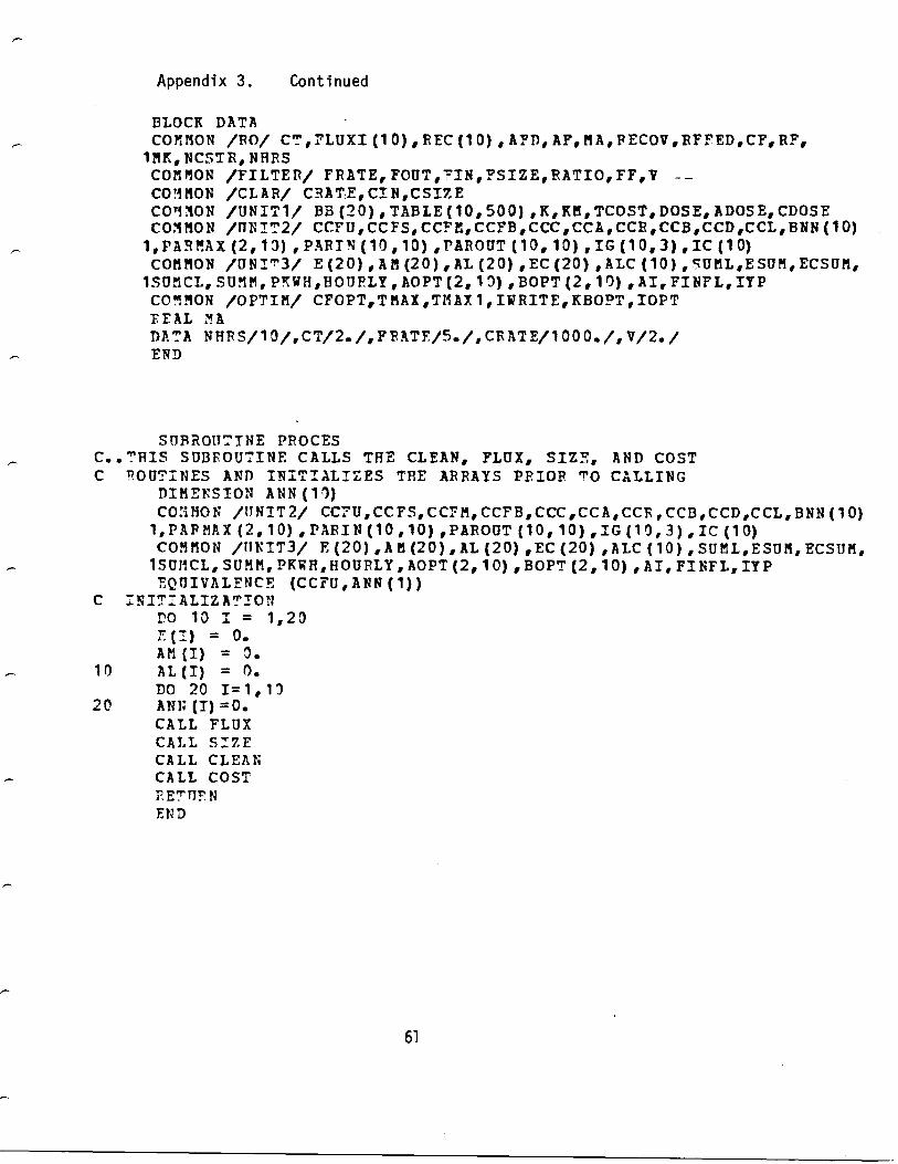
Appendix 3 .

Continued

BLOCK DATACOMMON /PO/ C"_', F LUXI (10) , REC (10) , AFD, AF, MA, PECOV, RFFED,CF, RF,1MK,NCSTR,NHRSCOMMON /FILTER/ FRATE,FOUT,='IN,FSIZE,RATIO,FF,V --COMMON /CLAP/ CRAT:E,CIN,CSIZECOTi10N /UNIT1/ BB (20) ,TABLE (10, 500) , K, KM,TCOST, DOSE, ADOSE, CDOSECOMMON /TTNIT2/ CCFU,CCFS,CCFI;,CCFB,CCC,CCA,CCR,CCB,CCD,CCL,BNN(10)1,PARY':AX(2,13),PARIN(10,10),PAROUT(10,10),IG(10,3),IC(10)COMMON /UNIT3/ E(20),AM(20),AL(20),EC(20),ALC(10),SUML,ESUM,ECSUM,1SUMCL, SU"]M, PRWH,HOURLY, AOPT (2, 10) ,BOPT (2, 10) , AI, FINFL, IYPCOMMON /OPTIM/ CFOPT,TMAX,TMAX1,IWRITE,KBOPT,IOPTREAL :!ADATA NHRS/10/,CT/2 ./,FRATE/5 ./,CRATE/1000 ./,V/2./END

SUBROUTINE PROCESC . .THIS SUBROUTINE CALLS THE CLEAN, FLUX, SIZE, AND COSTC ROUTINES AND INITIALIZES THE ARRAYS PRIOR TO CALLING

DIMENSION ANN(10)COMMON /IINIT2/ CC U,CCFS,CCPM,CCFB,CCC,CCA,CCR,CCB,CCD,CCL,BNN(10)1,PAFMAX (2, 10) , PARIN (10, 10) ,PAROUT (10, 10),IG (10,3),IC (10)COMMON /TINIT3/ E (20) ,A M (20) , AL (20) ,EC (20) , ALC (10) , SUML,ESUM, ECSUM,1SUJlCL, SUMM, PKWH,HOURLY, AOPT (2, 10) , BOPT (2, 10) , AI, FINFL, IYPEQUIVALENCE (CCFU, ANN (1) )

C INITIALIZAT_TONP0 10 I = 1,20

AM (I) = 0 .10

AL (I) _ 0 .DO 20 1=1,11

20 ANN (I) =0.CALL FLUXCALL S_ZFCALL CLEANCALL COSTi E?' ?'TIF NEND

61

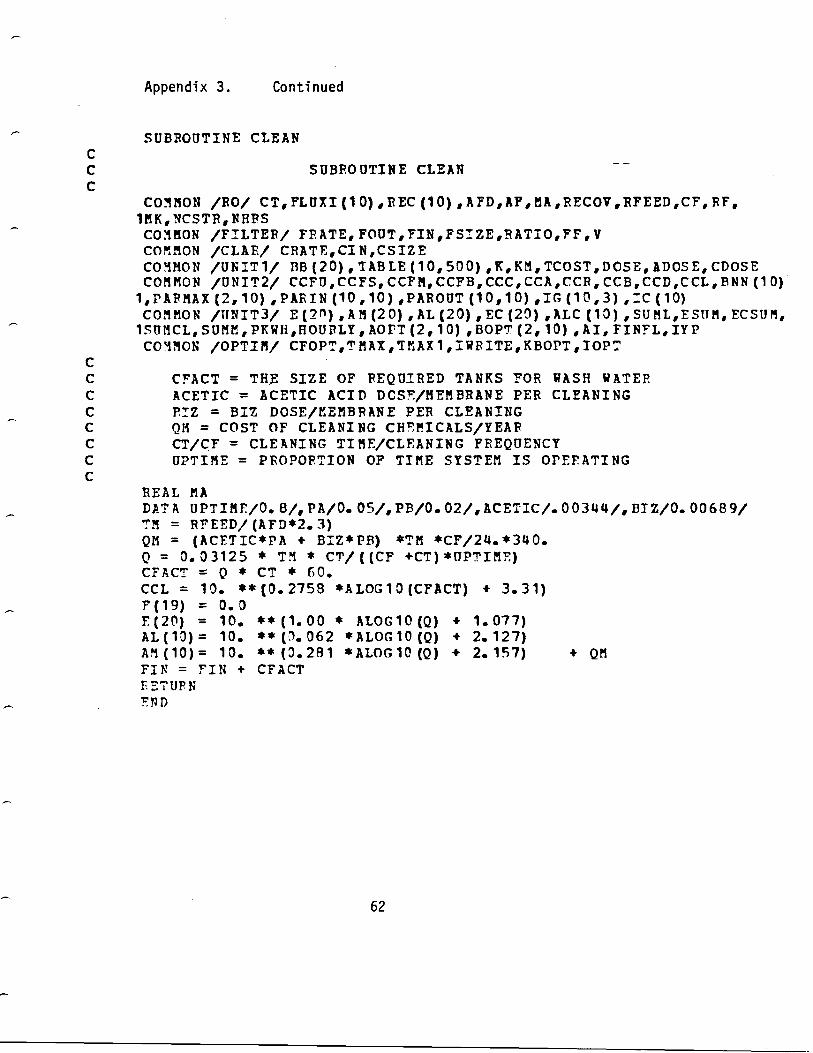
Appendix 3 .

Continued

SUBROUTINE CLEANCC

SUBROUTINE CLEANC

COMMON /RO/ CT,FLUXI(10),REC(10),AFD,AF,MA,RECOV,RFEED,CF,RF,

62

1NK,NCSTR,NHPSCOMMON /FILTER/ FRATE,FOUT,FIN,FSIZE,RATIO,FF,VCOMMON /CLAF/ CRATE,CIN,CSIZECOMMON /UNIT1/ BB(20),TABLE(10,500),K,KM,TCOST,DOSE,ADOSE,CDOSECOMMON /UNIT2/ CCFU,CCFS,CCFM,CCFB,CCC,CCA,CCR,CCB,CCD,CCL,BNN(10)1,PAPMAX (2,10) ,PARIN (10,10) ,PAROUT (10,10) ,IG (10,3) ,-C (10)COMMON /UNIT3/ E (2n) AM (20) , AL (20) EC (20) ALC (10) , SUML,ESTTM, ECSUM,1SUMCL, SUMM, PKWH,HOUPLY, AOFT (2, 10) , BOPT (2, 10) , AI, FINFL, IYPCOMMON /OPTIM/ CFOPT,TMAX,TMAX1,IWRITE,KBOPT,IOPT

CCCCCCCC

CFACT = THE SIZE OF REQUIRED TANKS FOR WASH WATEPACETIC = ACETIC ACID DCSF/MEMBRANE PER CLEANINGPIZ = BIZ DOSE/LEMBRANE PER CLEANINGQM = COST OF CLEANING CH…MICALS/YEARCT/CF = CLEANING TIME/CLEANING FREQUENCYUPTIME = PROPORTION OF TIME SYSTEM IS OPERATING

REAL MADATA UPTIMF./0 .8/,PA/0.05/,PB/0.02/,ACETIC/.00344/,BIZ/0.00689/711 = RFEED/ (AFD*2. 3)QM = (ACETIC*PA + BIZ*PB) *TM *CF/24.*340 .Q = 0 .03125 * TM * CT/ ((CF +CT) *UPTIME)CFACT = Q * CT * (0 .CCL = 10 . **(0 .2758 *ALOG10 (CFACT) + 3 .31)F(19) = 0.0F(20) = 10 . **(l .,00 * ALOG10 (Q) + 1 .077)AL (10) = 10 . **( .1.062 *ALOG 10 (Q) + 2.127)AM (10) = 10 . **(0 .281 * ALOG 10 (Q) + 2.157) + QMFIN = FIN +FETUPNEND

CFACT

Appendix 3 .

Continued

SUBROUTINE FLUX

SUBROUTINE FLUX

„

FSUM IS THE TOTAL FLOW BETWEEN CLEANINGS„

CF = THE CLEANING FREQUENCY„

CT = CLEANING TIME„

FLi1XI = FLUX A? 'ER CLEANING„

FRC = THE RECOVERY AFTER CLEANING„

FSRM/TOTAL TIME = AVERAGE FLUXDIMENSION F (500),T (500) ,Z (102) ,AAF (500)COMMON /BO/ CT,FLUXI(10),FEC(10),AFD,AF,MA,IlECOV,RFEED,CF,RF,1MK, NCSTP, NHRSCOMMON /FILTER/ FEATE,FOUT,FIN,FSIZE,RATIO,FF,VCOMMO! /CLAP/ CRATE,CIN,CSI7ECOMMON /UNIT1/ BB(20),TABLE(10,500),K,KM,TCOST,DOSE,ADOSE,CDOSECOMMON /UNIT2/ CCFU,CCFS,CCFM,CCFB,CCC,CCA,CCR,CCB,CCD,CCL,ANN(10)1,PAFMAX (2, 10) , PARIN (10,10) ,PAROUT (10, 10) , IG (10,3) , IC (1 0)RrAL MAFMAX = 0 .0FSUI = 0.KK = CF+D.5F(1) = FLUXI(KM)N = KK +1DO 10 ' = 2,NF (T) = FLUXI (KM) * (1 . /FLOA^' (I) **BB (KM) )FSUN = FSUM + (F (I) + F (I-1)) /2 .

10 CON .rINUEAF = FSUM/ (KK + CT)R…COQ = AF * REC(KM)/FLUXI (KM)AFD = AFCF = FLOAT (KK)R TURNEND

63

Appendix 3 .

Continued

SUBROUTINE BLENDCC

SUBROUTINE BLENDCC

COMMON /90/ CT,FLUXI (10),REC (10) ,AFD,AF,MA,EFCOV,RFEED,CF,RF,1MK,NCSTR,NHRSCOMMON /FILTER/ FFATE,FOUT,FIN,FSIZE,RATIO,FF,VCOMMON /CLAP/ CRATE,CIN,CSIZECOMMON /UN! 1/ BB(20),TABLE(10,500),K,KM,TCOST,DOSE,ADOSE,CDOSECOMMON /UNIT2/ CCFU,CCFS,CCFM,CCFB,CCC,CCA,CCR,CCB,CCD,CCL,BNN(10)1,PAR1!AX (2, 10) PARIN (10,10) ,PAROUT (10, 10) IG (10,3) :[C(10)COMMON /OPTIM/ CFOPT,TMAX,ZMAX1,IWRITE,KBOPT,IOPTF…AL MAPATIOM = .0KK = 1

C LOOP ?OF CALCULATING THE BLENDING RATIO. FIRST FIND THF CONTROLLINGC WATER QUALITY PARAMETER

DO 10 K=1, NCSTRC . . CHECK ^'0 SEP IF BLENDING IS REQUIRED. BYPASS RATIO CALCULATIONSC

'F BLEND:NG IS NOT REQUIRED .IF (PARIN (KM,K) . LE. PARMAX (1,K)) GOTO 10RATIO = (PARMAX (1, K) - PARIN (KM, K)) / (PAROUT (KM, K) - PARIN (KM, K) )IF (PATIO. L-. RATIOM) GO TO 10RATIOM = RATIOKK = K

13

CONTINUEC PRINT-OUT OF BLENDED PATIOS

RATIO = PATIOMDO 2n I = 1,NCSTR

20

PARMAX (2,I) = (PATIO*PAROUT (KM,I)) + ((1 .-RATIO) * PARIN (KM,I) )WRITE (6, 1000) IC (KK) ,K M,BB (KM) , (=C (K) ,PARIN (KM, K) , PAROUT (K M, K)

1, (DT,R"AX (I, K) , I=1, 2) , K=1, NCSTR)1000 FORMAT(///,T20,'THE LIMITING PARAMETER IS ',A3,' FOR B(',I1,')=',

1F6 .3,///,T20,'THE FOLLOWING WATER QUALITY RESULTS',/,T20,2'FILTER','"33,'PO ',T40,'F'QUIRED',T50,'BLENDED',34 (/,T10,A3,T19,F8 . 1,T26,F8 .1,T39,F8 . 1,T50,•8 . 1) )WRITF (6, 1010) RATIO

1010 FORMAT(//,' '"HE RATIO OF BLENDED PO PRODUCT WATER TO TOTAL',1' PRODUCT FLOW = "F5 .3)RETURN'N D

64

Appendix 3 .

Continued

SUBPOUTINE READERC . . THIS SUBPOUTINE READS THE INPUT DATA THEN WRITES OUT THE STARTINGC . . VALUES OF B, INITIAL FLUXES, AND TREATMENT OBJECTIVES

COMMON /RO/ CT,FLUXI(10),REC(10),AFD,AF,MA,RECOV,PFEED,CF,RF,1FK,NCSTP,WHESCOMMON /FILTER/ FRATE,FOUT,FIN,FSIZE,RATIO,FF,VCOMMON /CLAR/ CRATE,CIN,CSI!ECOMMON /UNIT 1/ BB (20) ,TABLE (10, 500) , K, KM,TCOST, DOSE, ADOSE, CDOSECOMMON /UNIT2/ CCFU,CCFS,CCFM,CCFB,CCC,CCA,CCP,CCB,CCD,CCL,BNN(10)1,PAEMAX (2,10) ,PARIN (10,10) ,PAROUT (10, 10) ,IG (10,3) ,IC (10)CCMMON /UNIT3/ E(20),AM(20),AL(20),EC(20),ALC(10),SUNL,FSUM,ECSUM,1SUi1CL, SU"lI, PKWH,HOURLY , AOPT (2, 10) , BOPT (2,10) , AI, FINFL,IYPCOMMON /OPTIM/ CFOPT,TMAX,TMAX1,IWRITE,KBOPT,IOPTDIMENSION AIA (5), :YEAP (5) ,FINFLA (5) ,PKWHA (5)REAL MA,LABORC (5)DATA IYEAFB/1979/

C . . READ THE NUMBER OF FLUX DECLINE ALTERNATIVESFEAD (5, 1000) MK

1000 FORMAT (I2)C. . WRITE OUT THE NUMBER OF ALTERNATIVES

WRITE (6, 1010) MK1010 FORMAT (' 1 THE NUMBER OF ALTERNATIVES IS ',I2)C . . PEAD THE NUMBER OF FINISH WATER QUALITY CONSTRAINTS

FEAD (5,.1000) NCSTRC. . WRIT :: OUT THE NUMBER OF CONSTRAINTS

WPI"E (6, 1020) NCSTR1020 FORNAT('OTHE NUMBER OF WATER QUALITY PARAMETERS IS ',I2)C. . READ AND WRITE THE PARAMETER AND ITS MAXIMUM VALUE

WRITE (6,1030)1030 FORMAT(T21,'WATER QUALITY OBJECTIVES',//,' PARAMETER',

1T15,'MAXIMUM VALUE')DO 10 I=1, NCST RPEA D(5, 1040) IC (I) ,PARMAX (1,I)

1040 FORMA - (A4, 6X, F 10 . 0)10

WRITE (6, 1050) IC (I) ,PARMAX (1,I)1050 FORMAT (T6,A4,T18,F10 .2)C . . PEAR THE INPUT DATA FOR EACH ALTERNATIVE

LOOP=O20

LOOP= :.OOP+ 1IF(LOOP-MK) 30,33,60

C. . READ THE B VALUES, INITIAL FLUXES AND RECOVERIES, AND WATER QUALITYC

OBJECTIVES .C. . CHECK TO SEE IF THE REQUIRED VALUES ARE SUPPLIED VALUES AREC

CONSISTENT WITH THE MAXIMUM VALUES30

FEAD (5, 1')6l)) BB (LOOP), REC (LOOP) FLUXI (LOOP)1360 -OP .tAT (P^13 .3)

PEAD(5, 1^63) (PARIN (LOO?,J),J=1,NCSTR)READ (5, 1'60)

(?AFOUT (LOOP,J) ,J=1,NCSTF)C. . CHECK TO SSP IF THE RO PRODUCT WATER QUALITY EXCEED THE REQUIFEP

DO 40 J=1, NCSTRIF (PAROUT (LOOP, J) . LE . PARMAX (1,J) ) GOTO 50

40

CONT NUEC . . AN UN…….ASIRLp ALTERNATIVE HAS 13FFN SELECTED . WRITE OUT AN ERRORC . . MESSAGE ANT) STOP

65

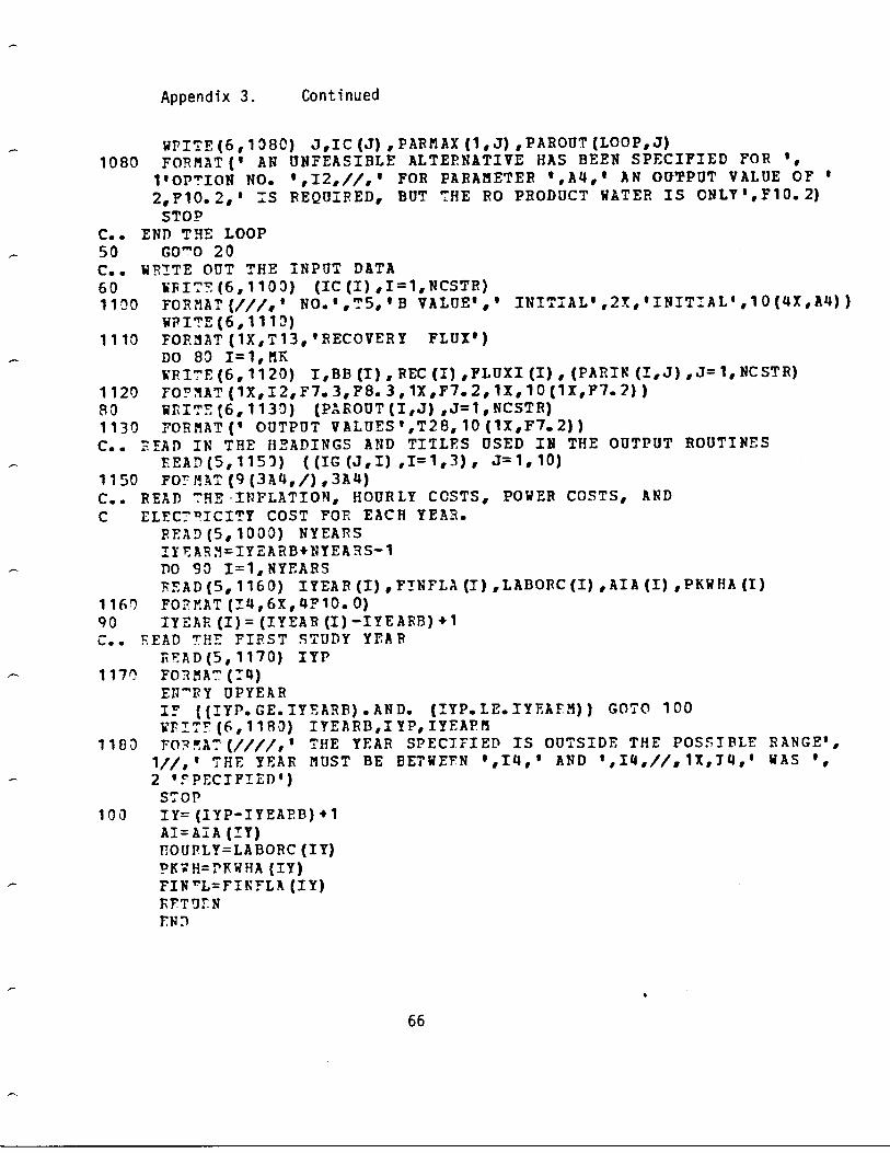
Appendix 3 .

Continued

WPITE(6, 1080) J,IC (J) , PARK AX (1,J) PAROUT (LOOP,J)1080 FORMAT(' AN UNFEASIBLE ALTEPNATIVE HAS BEEN SPECIFIED FOR ',

1'OPTION NO . ',I2,//,' FOR PARAMETER ',A4,' AN OUTPUT VALUE OF '2,F10 .2,' 1S REQUIRED, BUT THE RO PRODUCT WATER IS ONLY',F10.2)STOP

C. . END THE LOOP50

GO'"O 20C. . WRITE OUT THE INPUT DATA60

WFI:'E (6, 1100) (IC (I) ,I=1,NCSTR)1100 FORMAT(///,' NO .',TS,'B VALUE',' INITIAL',2X,'INIT'-rAL',10(4X,A4))

WRITE (6, 1110)1110 FORMAT (1X, T 13,' RECOVER Y FLUX')

DO 80 I=1, MKWRITE (6, 1120) I,BB (I) , REC (I) ,FLUXI (I) , (PARIN (I_,J) ,J= 1, NCSTR)

1120 FO…`tAT (1X,I2,F7 .3,F8.3, 1X,F7.2, 1X,10 (1X,F7 .2) )80

WRITE (6,1130) (PAI ROUT (I,J) ,J=1, NCSTR)1130 FORMAT (l OUTPUT VALUES',T28, 10 (1X,F7.2) )C. . R EAD IN THE READINGS AND TITLES USED IN THE OUTPUT ROUTINES

FEAD (5, 115)) ((IG (J,I) ,I=1,3) , J=1, 10)1150 FORMAT (9 (3A4,/) 3A4)C . . READ THE-INFLATION, HOURLY CCSTS, POWER COSTS, ANDC

ELFC'DICITY COST FOR EACH YEAR .READ (5, 1000) NYEARSIY EAR`t=IYEARB+NYEARS-1DO 90 I=1,NYEARSFEAD (5, 1160) IYEAR (I) , FINFLA (I) ,LABORC (I) ,AIA (I) ,PKWHA (I)

1160 FORMAT (T_4,6X,4F10 .0)90

IYEAR (I) = (IYEAR (I) -IYEARB) +1~ . . READ THE FIRST STUDY YEAR

READ (5, 1170) IYP1170 FORMAT (I4)

EN- FY UPYEARIF (( I YP. G E.IYEARB) . AND. (IYP. LE.IYEAFM)) GOTO 100VPITE (6,11 R0) IYEARB,I YP, IYEAPM

1180 FO?":A"_' (////,' THE YEAR SPECIFIED IS OUTSIDE THE POSSIBLE RANGE',1//,' THE YEAR MUST BE BETWEEN ',I4,' AND ',14,//,1X,74,' WAS ',2 'SPECIFIED')SWOP

100

IY=(IYP-IYEARB)+1AI =Al A (I Y)1?OUPLY=LABORC (IY)PKWH=PKWHA (IY)FIN"L=FISFLA (IY)FFT'J ::NEND

66

6 7

Appendix 3 .

SUBROUTINE SIZE

Continued

CCCC

SUBROUTINE SIZE

CALCULATES THE SIZES OF THE VARIOUS COMPONENTS OF THE SYSTEMCOMMON /FO/ CT,FLUXI (1 0),REC (10) ,AFD,AF,MA,PECOV,RFEED,CF, RF,1MF,NCSTR,NHRSCOMMON /FILTER/ FFATE,FOUT,FIN,FSIZE,FATIO,FF,VCOMMON /CLAP/ CRATE,CIN,CSIZECOMMON /UNIT2/ CCFU,CCFS,CCFN,CCFB,CCC,CCA,CCR,CCB,CCD,CCL,fNN(10)1,PARMAX (2,10) , PARI N (10,10) ,PAROUT (10, 10) , IG (10, 3) , IC (10)REAL MAA = 10.0**6

C BN = NUMBER OF BACKWASHES PER DAYFN = 2

C MEMBRANE AREA

AFD = AVERAGE FLUX/F72-DAY

MAMA = RATIO * A/AFD

C FFED FLOW RATE TO RO

RFEEDRFEED = PATIO * A/RECOV

C FILTER OUTPUT ROUT

CTOUT = EFEED + (1-RATIO) *A

(2%) FINFILTER INPUT = POUT + BACKWASH WATER

CFIN = ROUT

FILTER SURFACE AREA AT 5 GPM/FT2 FSIZE

C

FSIZE = FIN /(PRATE * 1440 .)

CSIZEFIN = FIN + BN*V*FSIZE

CLARIFIER AT 100 GPD/FT2CSIZE = FIN/1000 .RF .̂UFNEND

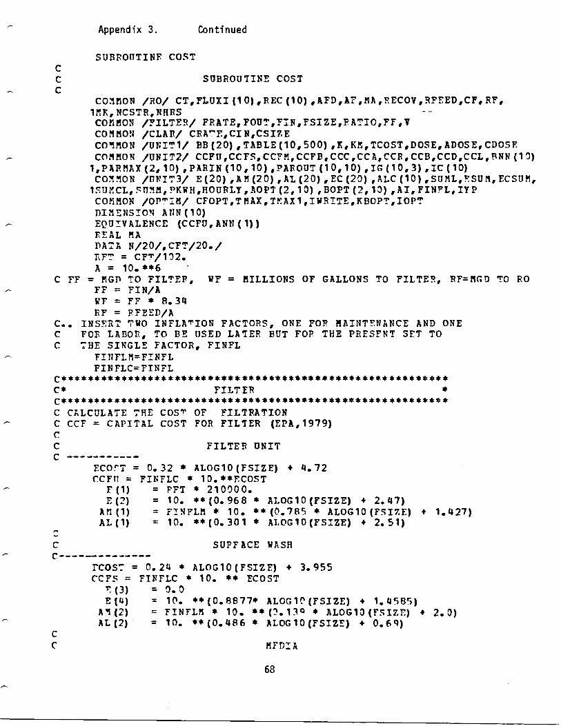
Appendix 3 .

Continued

SUBROUTINE COST

C

SUBROUTINE COST

COMMON /RO/ CT,FLUXI(10),REC(10),AFD,AF,MA,RECOV,RFEED,CF,RF,1MIC, NCSTR,NHRS

--COMMON /FILTER/ FRATE,FOUT,FIN,FSIZE,PATIO,FF,VCOMMON /CLAP/ CRA-E,CIN,CSIZECOMMON /UNIT1/ BB(20),TABLE(10,500),K,KMM,TCOST,DOSE,ADOSE,CDOSECOMMON /UNIT2/ CCFU,CCFS,CCFM,CCFB,CCC,CCA,CCR,CCB,CCD,CCL,BNN(10)1,PARMAX (2, 10) , PARIN (10, 10) ,PAROUT (10, 10) , IG (10, 3) ,IC (10)COMMON /UNIT3/ E (20) ,AM (20) , AL (20) , EC (20) ,ALC (10) ,SUML,F:SUM, ECSUM,1SUrCL, SDMM, PKWH,HOURLY, AOPT (2, 10) , BOPT (2, 13) , AI, FINFL, IYPCOMMON /OP-T-H/ CFOPT,TMAX,TMAX1,IWRITE,KBOPTT,IOPTDIMENSION AKIN (10)EQUIVALENCE (CCFU, ANN (1) )REAL MADATA N/20/,CFT/20 . /T.FT = CFT/ 102 .A = 10 . **6

C FF = MGP TO FILTER, WF = MILLIONS OF GALLONS TO FILTER, RF=MGD TO POFF = FIN/AVF = FF * 8 .34RF = FFEED/A

C . . INSERT TWO INFLATION FACTORS, ONE FOP MAINTENANCE AND ONEC

FOB LABOR, TO BE USED LATER BUT FOP THE PRESENT SFT TOC THE SINGLE FACTOR, FINFL

FINFLM=FINFLFINFLC=FINFL

C**********************************************************C* FILTER *C**********************************************************C CALCULATE ;'HE COST OF FILTRATIONC CCF = CAPITAL COST FOR FILTER (EPA,1979)CC

FILTER UNITC

ECOrT = 0 .32 * ALOG10 (FSIZE) + 4 .72CCFU = FINFLC * 10 . **FCOST

„

(l) = FFT * 210000 .„

(2) = 10 . **(0 .968 * ALOG10 (FSIZE) + 2 .47)AM (1)

= FINFLM * 10 . ** (0 .785 * ALOG10 (FSIZE) + 1 .427)AL (1)

= 10. **(0.301 * ALOG10 (FSIZE) + 2.51)

C

SURFACE WASHC

rcosT = 0.24 * ALOG10 (FSIZE) + 3 .955CCFS = FINFLC * 10 . ** ECOST

„

(3) = 0.0„

(4) = 10. **(0 .8877* ALOG1O (FSIZE) + 1 .4585)Ay (2)

= FINFLM * 10 . ** (1 . 13Q * ALOG10 (FSIZE) + 2 . 0)AL (2)

= 10. **(0 .486 * ALOG 10 (FSIZE) + 0.6q)CC

MFDIA

68

Appendix 3 .

Continued

cCC:'M = FINFLC * 10 . **(0 .652 * ALOG 10 (FSIZE) + 2 .554)

„

(5) = 0 .„

(6) = 0A11 (3) = FINFLM

AL (3) = 0 .CC

BACKWASHC

Q = FSIZE * V * 7 .48CCFB = FINFLC * 10 . **(0.37 * ALOG 10 (Q) + 3.49)

„

(7) = 0.0„

(8) = 10. **(1 .00 * ALOG10 (FSIZE) + 1 .38)AL (4)

= 10. **(0 .062 * ALOG10 (FSIZE) + 2.146)AM (4)

= FINFLN * 10 . **(0 .281 * ALOG10 (FSIZE) + 2 .24)CC

TOTAL CAPITAL COST FOR FILTER (CCF)C

CCF = CCFU + CCFS + CCFM + CCFBC IF PFETREATMFNT INCLUDES MORE THAN FILTEATION GO TO 10C*************************************************************C*

CLARIFIER

*C*************************************************************C OVERFLOW = 1000 . GPD/FT2C CCC = CLARIFIFR CAPITAL COSTSC CCA = CAPITAL COSTS FOR CHEMICAL FEED SYSTEMSCC

CLARIFIER UNIT

C. . BY PASS THE COST CALCULATIONS FOR THE OPTIONS WITHOUTC

COAGULATION K9= 4 OR 6

A103) = FINFLM * 10 . **(0.640 * ALOG10 (CSIZE) + 0 .574)CC

COAGULANTSC

B ::ANCH TO THE PROPER CHEMICAL FEEDC1 5

GO TO (20, 25, 30,35, 20, 35, 30, 35) ,KMCC

NALCO 7134 & 1OPPMC

25 CCA = FINFLC * 20200 .DOSE = 5PR? C… = 1 .50AMT = V7 * DOSE * PPICE*340 .

„

(11)= FFT * 8210.„

(12)= 17300 .AL (6) = 1n!) .Al (6) = Fi!P'LM * 270. + AMT

69

IF ((K M. EQ. 4) OR. (K N . EQ .6)) GOTO 1510 FCOST = 0 . 322 * ALOG 10 (CSIZE) + 4 . 01

CCC = FINFLC * 10 . ** ECOSTF (g) = 3.0E(10)= 10. **(0.172 * ALOG10 (CSIZE) + 3.024)

AL (5) = 10 . **(0 .154 * ALOG1 O (CSIZE) + 1 .736)

Appendix 3 .

Continued

K = 2GO TO 40

CC

FECL3 a 50 PPMC

20 DOSE = 50AM'." = WF * DOSE/24 .PRICE = .10CCA = FINFLC * 10 . **(0 .278 * ALOG10 (AMT) + 4 .00)„

(11) = FFT * (10 . ** ( .574 * ALOG10 (AMT) + 3. 20) )„

(12) = 4900.AL (6) = 13. ** (0 . 062 * ALOr,10 (AMT) + 2 . 396)AM (6) = 1r). **(0.067 * ALOG10 (AMT) + 2.186) + PFICE*AMT

K = 3GO TO 40

CC

ALUM a 60 PPMC

30 DOSE = 60CONC1 = .5PRICE = .05AMT = RF * DOSE/24 .AM - C = AMT/CONC1CCA = FINFLC * 10 . ** (0.232 * ALOG 10 (AMTC) + 4 .08)„

(11) = FFT * (10 . ** (0.574 * ALOG10 (AMT) + 3. 216) )F (12) = 4913 .AL (6) = 10 . **(0.062 * ALOG10 (AMT) + 3.97)A'". (6) = FINFLM * (200 . + PRICE * ART)

K = 4GO TO 40

35 K=1C

NO CHEMICALSC

CHEMICAL COSTS HAVE BEEN INITIALIZED TO ZERO IN MAIN ROUTINECC*ssss**********************s*************************s*********C*

REVERSE OSMOSISC*********s*********************************************s*s****sC CCF = CAPITAL COSTSC

40 CCR = FINFLC * 10 . **(0 .848 * ALOG10 (RF) + 5.89)E(13) = RFT * (10 . **(0 .901 * ALOG10 (RF) + 5 .023))F(14) = 10 . **(0.962 * ALOG 10 (RF) + 6.382)AL (7) = 10 . **(0.188 * ALOG10 (RF) + 3.265)AM (7) = FINFLM * 10 . **(0 .886 * ALOG10 (RF) + 4 .988)

CC

FRFTREA'rNENT CHEMICALSCC

SULFURIC ACIDC

CONC = 0 .96FR'C1 = 7 .40ADO -SE = 15 .1/1 .9318AMT = APOSE * FF/CONCCCf = FINFLC * 10 . **(0 .1186 * ALOG10 (AM :") + 3 .S2)

7 0

Appendix 3 .

Continued

E(15) = RFT * 3680 .E(16) = 1630 .AL (8) = 10 . ** (0. 330 * ALOG10 (AM 7) + 1 . 53)AM (8) = FINFLM* (10 . **(0 .222 * ALOG10 (AMT) +1 .56) +PRIC1 *AMT)

CC

CHLORINEC

IF (K. GT . 1) CDOSE = 2 .IF (K. LE. 1) CDOSE = 9 .FPIC2 = 0 .25AMT2 = AF * CDOSE/24 .

CC*************************************************************C************* TOTAL COSTS *******************************C*************************************************************C

CC-

SUML = 0 .i:SUM = 0 .SUM'S = 0 .ECSUM = 0 .SUMCL = 0 .no 50 I = 1,20r.C (I) = E (I) * PKWHESUM = ESUM + 11" (1)ECSUM = ECSU9 + EC (I)

50 CON'"INUFDO 60 J = 1,10ALC (J) = AL (J) * HOURLYSU1L = SUML + AL (J)SUMCL = SUMCL + ALC (J)SUrr. = SUMM + AM (J)

60 CON"INUETOTAL CAPITAL (TCAP) AND OSM (TOM) COSTS

------------------TCAr = CCF + CCC + CCA + CCF + CCD + CCD +CCL".'0"I =

SUMM + SUNCL + ECSUMCC

ANNUAL CAPITAL COSTSC

AT = (1 + AT) **Nr

_ ( AI * AT)/ (AT

1)no 7') I = 1,10BNN (_) = ANN (I) * F

70

CONTINuIEACAP = TCAr * FTCO_ T = TOM + ACAPIr("COST .G T."NAR1) GO^_0 78

C. . TENS RT „'ANCH 73 TARE' IF THE Pr ESEN .̂ CLEANING rR'QFUFNCYC

A LOW 7-r TOTAL COST

71

GI VES

CCD = FINFLC * 10 . **(0 .3625 * ALOG 10 (AMT2) + 3 .752)E(17) = 13 . **(0 .517 * ALOG 10 (AMT2) + 3 .448)F(18) = 10 . **(0 .173 * ALOC,10 (AMT2) + 2 .58)

AL (9)

= 10. **(0 .1066 * ALOG10 (AMT2) + 2.53)AM (9) = FINFLM* (10.** (0.177*ALOG10 (AKT2) +2 .570) +PRIC2*AMT2)

Appendix 3 .

Continued .

DO 75 I = 1, 10EOP' (1,I) = EC (2*1-1) +EC (2*1) + ALC(I) + AM (I)

75

AOPT (1, I) = (BNN (I) +BOPT (1, I)) /340000 .C

SELECT LEAST TOTAL ANNUAL COSTCC

TCAXI=TCOST78

IT ( TCOST.L T. TMAX) GO TO AOFETaRN

C . . THIS BRANCH IS TAKEN IF THE LOWEST COST FOR THE OPTIMAL CLEANINGC

FREQUENCY FOR THIS B VALUE IS THE LOWEST SO FAR IN THE ANALYSISC

THAX IS THE GLOBAL OPTIMUM80

KBOPT = 'KMCOPT = CFT!!AX = TCOSTPO 90 i- 1,10BOFT (2,I) = EC (2*I-1) +EC (2*I) + ALC (I) + AM (I)

93

AOPT (2,I) = (}3NN (I) +BOPT (2,I) )/340003.PFTUPNEN')

7 2

Appendix 3 .

Continued

SUBROU'T'INE OUTPUT (CFE)CC

SUBROUTINE OUTPUT

-C

COMMON /OPTIM/ CFOPT,TMAX,TMAX1,IWRITE,KBOPT,IOPTCOMMON /RO/ CT,FLUXI(10),REC(10),AFD,AF,MA,RECOV,RFEED,CF,RF,1MK,NCSTR,NHPSCOMMON /FILTER/ FRATE,FOUT,FIN,FSIZE,RATIO,FF,VCOMMON /CLAR/ CRATE,CIN,CSIZECOMMON /UNIT1/ BB (20) ,TABLE (10,500) ,K,KM,TCOST,DOSE,AROSE, CDOSECOMMON /UNIT2/ BN (10) , BNN (10)

1,PARMAX (2, 10) ,PAR=N (10,10) ,PAROUT (10, 10) ,IG (10, 3) ,IC (10)COMMON /UNIT3/ E(20) A M (20) AL (20) , EC (20) ALC (10) , SUML,ESUM, ECSUM,1SUMCL, SUP:M, PKWH, HOUPLY, AOPT (2, 10) , BOPT (2, 10) , ?iI, FINFL, IYPDIMENSION AA (4,3)DA^A AA/'

',' NA „, 'LCO ','7134',' FEE','RIC ','CHLO','RIDE',1'

o,'

','

„, 'ALUM'/REAL MA

C READ IN THE NAMES OF THE UNIT PROCESSES ; COLS 2-17= PRESSURE FILTERC COLS 1a-34= CLARIFIER, COLS 36-51= CHEMICAL FEED, COLS 53-68 =C RFVEP F. OSMOSISC ASSUMETIONS

PA'=100*AIWRI-E(6,223) HOURLY,PKWH,PAI,FINFL,IYP

220 FORMAT(///,T40,'ASSUMPTIONS',/,T30,'LABOR RATE = $', F6 .2,' PER HOU1F ',//,T25,'ELECTRICAL RATE = $',F6 .2,' PER KWH',//,T26,'INTEFEST2FA^" = ', F7.2,'%',//,T25,'LIFE OF PROJECT =

20 YEARS',//,3T25,'iNFLATION PATIO =',F10.3,//,T28,'PROJECT YEAR = ',I9)

C***********************************************************************C

TABLE OF ANNUAL COSTS AND FLUX DECLINE INDEXCC TABLE HEADINGSC

W'PITE (6, 10) (I,1=1,40,4)C 10 FOFYAT(/////,T20,'TOTAL ANNUAL COSTS FOR VARYING VALUES OF THE FLUC

1X PECLINE INDEX (B) AND THE CLEANING INTERVAL',//,T50,C

2'CLEANING INTERVAL (HOURS)',/,T3,'R',T5, 10110)CC B VALUES AND TOTAL ANNUAL COSTS

C

P VALUES AND COSTS PER THOUSAND GALLONSDO 30 J = 1,NHRSTABLE (KM,J) = TABLE (KM,J) /340000 .

33 CON'"TNUEIcF=c"F* 0 . 5ICE"'=ICF*NHtSWP?T'„: (6, 40) (I, -L=ICF, ICFT, ICF)

4? FORMAT(////,T10,'COSTS PER GALS FOR VARYING VALUES OF P AND THE C1LEANING IN .̂EEVAL',//,T30,'CLEANING INTERVAL (HOURS) ',/TR,'B',T10,213 :()W^ :^F (f ,S?) BB (KM), (TABLE (KM,J) ,J=1, 10)

50 rc' Rrr,^ (/,^5, F5 . 2,'"10, 1 0F6 . 2)C,*###*******#****************#**********#***#*****#*##***#********#

7 3

C WRITE (6,23) (BB (I) , (TABLE (I,J) 3=1,10) ,I=1,MK)CC

20 FOF`iAT (/, (F 5. 2,T10, 10 (F9 .0, 1X)) )

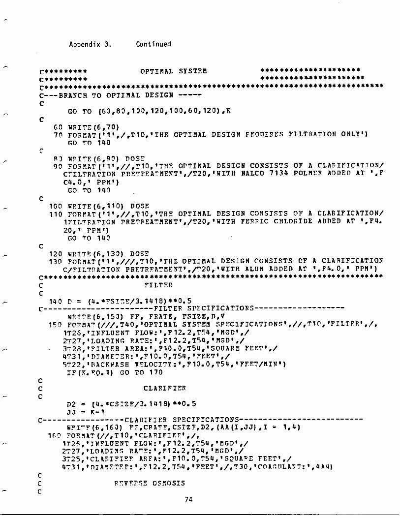
Appendix 3 .

Continued

C*********

OPTIMAL SYSTEM ************* *******C*********

**********#***********C**************************************~********************************C---BRANCH TO OPTIMAL DESIGNC

GO TO (63,80,100,120,103,60,120),KC

60 WRITE (6,70)7f) FORr.AT (' 1',/,T10,'THE OPTIMAL DESIGN REQUIRES FILTRATION ONLY')

GO TO 140C

R3 WRITE (6,90) DOSE90 FORMAT (' 1',//,Tl0,' :'HE OPTIMAL DESIGN CONSISTS OF A CLAFIFICATION/

CrILTRATION PRETPEAT'MENT',/T20,'WITH NALCO 7134 POLMER ADDED AT ',FC4 .3, 1 PPM')GO TO 140

C100 WRITE (6, 110) DOSE110 FORMAT (' 1',//,T10,'THE OPTIMAL DESIGN CONSISTS OF A CLARIFICATION/

1FILTFATION PRETREATMENT',/T20,'WITH FERRIC CHLORIDE ADDED AT ',F4.20,' PPM')GO TO 140

C120 WRITF (F, 130) DOSE130 FORMAT('1',///,T10,'THE OPTIMAL DESIGN CONSISTS CF A CLARIFICATION

C/FILTRATION PRETRFATMENT',/T20,'WITH ALUM ADDED AT ',F4.0,' PPM')C***********************************************************************C

FILTERC

140 D = (4 . *FSI F/3 . 1418) * *0 .5C FILTER SPECIFICATIONS

WRITE (6, 153) FF, FRATE, FSIZE, D,Y150 FORMAT (///,T40,'OPTIMAL SYSTEM SPECIFICATIONS',//,T10,'FILTFR',/,

1T26,'INFLUENT FLOW :',F 12. 2,T54,'MGD',/2T27,'LOADING RATE:',F12.2,T54,'MGD',/3728 . 1-FILTER AREA:',F10 .0,T54,'SQUARE FEET',/4731,'D :AME'"ER :',F10 .0,T54,'FEET',/5T22,' BACKWASH VELOCITY :', F 10 . 0, T54,' FEET/MIN' )IF (K . FQ . 1) GO TO 170

CC

CLARIFIERC

D2 = (4. *CSIZE/3. 1418) **0 . 5JJ = K-1

C CLARIFIER SPECIFICATIONSW?I'-F (6,160) FF,CPATE, CSIZF,D2, (AA (I,JJ) , I = 1,4)

1(0 :=ORMAT. (//,T10,'CLARIFIEP',/,1T26,'IN…LUENT FLOW :',F12.2,T54,'MGD',/2':27,'LOADIN' RATE :',F12.2,T54,'MGD',/3T25,'CLAFIFIEF ARFA :',F10 .0,T54,'SQUApE FEET',/4731,'DIAIEirr :',?12 .2,T54,'FEET',/,T30,'COAc :(1LANT :',4A4)

CC

VERSE OSMOSISC

74

Appendix 3 .

Continued

170 PI-E" ECOV = R!;COV * 100 .Nl. = _FIX (RECOV * RFEED/(AFD*2 .3) )FFEED = RFEED/ (10 . **6)

CREVERSE OSMOSIS SPECIFICATIONSWRITE(6,180) RFEED.,RATIO,PRFCOV,BB(KBOPT),AFD,NN,N"A,CT

180 FORMAT(//,T10,'REVERSE OSMOSIS ',//,1726,' INFLUENT FLOW' :', F 12. 2,T54,' MGD' ,/,T27,' PRODUCT FLOW :' ,F 12 .2, T254,'MGD',/,T23,'PEFCENT P•COVEFY :',F12 .2,T54,'%',/,3T17,'FLUT DECLINE INDEX (B) :',F12.2,/,T27,'AVERAGE FLUX :',F12 .2,4^54,'GPn/FT2',/,T2'0,'NUMBER OF MEMBRANES :',I9,/,5T29,'TOTAL AREA :',F12 .2,T54,'SQUARE FEET',/,6T13,'TINE REQUIRED FOF CLEANING :',F12.1,T54,'HOURS')

CRO-CONTINUFDA==TE (6, 190) CF, ADOSE, CDOSE

190 FORMAT (l ' ,T22,'CLEANI NG INTERVAL :', F12. 1,T54,' 1TOURS' ,/,1T17,'SIILFUPIC ACID INJECTED :',F12.2,T54,'PPM',/,2T22,'CTILOPINR INJECTED :',F12.2,T54,'PPM')

C***********************************************************************C

TOTAL COSTSC***********************************************************************CHEADINGS FOR THE UNITS PROCESS COSTS

WRTTE (6,200)2'~') FOPMAT ('.1',///,T25,'FNERGY AND LABOR ANALYSIS',//,

1T13,'BUILPING ENERGY',2T35,'PFOCESS ENERGY',T55,'LABOR',/,3T12,'KWH/YR COST($/YR)',T32,'KWH/YR COST($/YR)',4T53,'HRS/YR S/YR')

CTOTAL AND ANNUAL COSTS OF UNIT PROCESSESC

UPI-:'E (6,213) (E (2*J-1) ,EC (2*J-1) ,E (2*J) ,EC (2*J) , AL (J)1,ALC(3),J=1,10)

21'? FOPMAT(/,T7,tFILTFR UNIT',6F9 .0,//,T6,'SUPFACE WASH',6FQ .0,1//,T13,'NFDIA',6F9 .0,//,T9,' BACKWASH',6F9 .0,//,2'T4,'CLARIFIEF UNIT',6F9 .0,//,T8,' COAGULANT',6F9 .0,//,3T3,'REVEFSF OSMOSIS',6F9 .0,//,4T5,'SULFi1RIC ACID',6F9 .0,//,T9,' CHLORINE',6F9 .0,//,5T10,'CLEANING',6r9.0)HFITF (6,214)

214 FOF"1AT (//,T35,'UNIT COSTS',//,T15,'TOTAL CAPITAL ($/YR)',T37,'ANNUA1L CAPITAL' ,T54, 4 0 & N (S/YF)',T67,"WATER COSTS ($/KCAL)')Wr-Tr (6, 215) ((IG (3,1) , I=1, 3) BN (J) , BNN (J) , BOPT (I OPT, J) ,1AOPT (IOPT, J) , J=1, 10)

215 FOR"1LT (/, 10 (T5,31 :4,T25,F8 .0,T45,F7.0,T60,F7.0,T75,F5.2,/))CAP = 0 .ECAP = 0 .DO 217 I = 1,10It' (I . GF.7) GO TO 216CAP = CAP + AOPT (IOPT, I)GO TO 21 7

216 FCAP = FCAP + AOPT (IOPT,I)217 CONTINUE

ADD = CAP + RCAPWFI'"r (6,219) CA-,FCP.P, Ann

213 For MAT(/,720,'COAGULATI01./CLARIFICATION/FILTRAT_ ON $/KGAL=',F5 .2,

7 5

Appendix 3 .

Continued

CKG = TMAX2/340000 .WRTTE(6,230) TMAX2,CKG

230 FORMAT(///,T15,' THE PLANT PRODUCES 1 MGD PER DAY OF THE SPECIFIED1 QUALITY WATEP',/,T10,'THE TOTAL ANNUAL COSTS = $',F9 .0,10X,2'COST/KGAL = $',F4 .2)rF"UENEND

SUBPOUTINE JDPLOTCOMMON /SCLP/FX,DX,FY,DY,ITFSTX,ITESTYDIMrNSION XVALS (100) YVALS (100) Z (105)DO 1 I = 1,10XVALS (I) = IYVALS (I) = I

1 CONTINUEDX = 8FX = 0EY = 1 . 0DY = .25I': E ST X = 1-.=--STY = 1

C

CALL CPLOTO (3, 10,-2,XVALS,YVALS, 1, 1,Z)PET URNEN n

7 6

1/,T10,'2/,T10,'

REVERSE OSMOSIS SYSTEM S/KGAL=',F5 .2,TOTAL SYSTEM E/KGAL=',F5 .2)

CCTOTAL COST AND PFICE/KGAL

TMAX2=TMAXIF ( IWFITE. NE .0) TMAX2=TMAX1