
Imprecise Inference Models in Decision Making and … · Imprecise Inference Models in Decision...
71
Imprecise Inference Models in Decision Making and Risk Analysis Lev Utkin, St.Petersburg September 2009, Munich
Transcript of Imprecise Inference Models in Decision Making and … · Imprecise Inference Models in Decision...

Imprecise Inference Models in Decision Making andRisk Analysis
Lev Utkin, St.Petersburg
September 2009, Munich

Imprecisely eight years ago

Precisely ve years ago

Precisely ve years ago

Precisely two months ago

Precisely two months ago

Best greetings and happy birhday from my family

Best greetings and happy birhday from my family

Best greetings and happy birhday from Saint-Petersburg

Best greetings and happy birhday from Saint-Petersburg

Best greetings and happy birhday from Saint-Petersburg

Best greetings and happy birhday from Saint-Petersburg

Bayesian Inference Models
Standard Bayesian Inference
1 Risk measure EX =R
Ω EaX π(ajb)da.2 Prior distribution π(ajb) of parameters a is our opinionabout the possible values a prior to collecting any information.
3 Set k = (k1, ..., kn) of observed events.
4 Likelihood function L(bjk) = p(k1ja) p(knja).5 Posterior distribution π(ajb, k) ∝ L(bjk) π(ajb) is ourupdated opinion about the possible values a.
Bayesian Inference Models
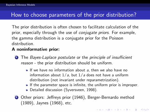
How to choose parameters of the prior distribution?
The prior distribution is often chosen to facilitate calculation of theprior, especially through the use of conjugate priors. For example,the gamma distribution is a conjugate prior for the Poissondistribution.A noninformative prior:
1 The Bayes-Laplace postulate or the principle of insucientreason - the prior distribution should be uniform.
If we have no information about a, then we also have noinformation about 1/a, but 1/a does not have a uniformdistribution (not invariant under reparametrization).If the parameter space is innite, the uniform prior is improper.Detailed discussion (Syversveen, 1998).
2 Other priors: Jereys prior (1946), Berger-Bernardo method(1989), Jaynes (1968), etc.

Imprecise models
Basis of imprecise models
A class of the noninformative prior models is based on dening aclassM of prior distributions π such that for event A
P(A) = inffPπ(A) : π 2 Mg, P(A) = supfPπ(A) : π 2 Mg.
\Not a class of reasonable priors, but a reasonable class of priors"
Walley's imprecise Dirichlet model (Walley 1996);
Walley's bounded derivative model (Walley 1997);
Imprecise models for inference in exponential families(Quaeghebeur, de Cooman 2005).
Imprecise Dirichlet model (IDM)
Dirichlet distribution
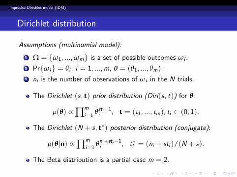
Assumptions (multinomial model):
1 Ω = fω1, ...,ωmg is a set of possible outcomes ωi .
2 Prfωig = θi , i = 1, ...,m, θ = (θ1, ..., θm).
3 ni is the number of observations of ωi in the N trials.
The Dirichlet (s, t) prior distribution (Diri(s, t)) for θ:
p(θ) ∝ ∏m
i=1θsti1i , t = (t1, ..., tm), ti 2 (0, 1).
The Dirichlet (N + s, t) posterior distribution (conjugate):
p(θjn) ∝ ∏m
i=1θni+sti1i , ti = (ni + sti )/(N + s).
The Beta distribution is a partial case m = 2.

Imprecise Dirichlet model (IDM)
Imprecise Dirichlet model (1)
The imprecise Dirichlet model (IDM) is (Walley 1996) the set ofall Dirichlet (s, t) distributions such that t 2 S(1,m).
The hyperparameter s determines how quickly upper and lowerprobabilities of events converge as statistical data accumulate.
Predictive probability of A
P(Ajn, t, s) = n(A) + st(A)
N + s,
n(A) = ∑ωi2Ani , t(A) = ∑ωi2A
ti .
Imprecise Dirichlet model (IDM)
Imprecise Dirichlet model (2)
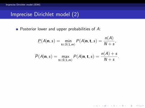
Posterior lower and upper probabilities of A:
P(Ajn, s) = mint2S(1,m)
P(Ajn, t, s) = n(A)
N + s,
P(Ajn, s) = maxt2S(1,m)
P(Ajn, t, s) = n(A) + s
N + s.
Before making any observations (vacuous model):
n(A) = N = 0,P(Ajn, s) = 0,P(Ajn, s) = 1.
We do not need to choose one specic prior.
Walley 1991,1996; Bernard 2001-06, Coolen 1997, Zaalon2002, Hutter 2003, Quaeghebeur, de Cooman 2005

Imprecise Dirichlet model (IDM)
Imprecise Dirichlet model (2)
Posterior lower and upper probabilities of A:
P(Ajn, s) = mint2S(1,m)
P(Ajn, t, s) = n(A)
N + s,
P(Ajn, s) = maxt2S(1,m)
P(Ajn, t, s) = n(A) + s
N + s.
Before making any observations (vacuous model):
n(A) = N = 0,P(Ajn, s) = 0,P(Ajn, s) = 1.
We do not need to choose one specic prior.
Walley 1991,1996; Bernard 2001-06, Coolen 1997, Zaalon2002, Hutter 2003, Quaeghebeur, de Cooman 2005

Imprecise Dirichlet model (IDM)
Successful applications of the IDM
1 Game-theoretic learning (Quaeghebeur, de Cooman 2003)
2 Credal treatment of missing data (Zaalon 2002)
3 Implicative analysis for multivariate binary data (Bernard2002)
4 Reliability analysis
Bayesian analysis of right-censored observations (Coolen 1997)Reliability analysis of multi-state and continuum-state systems(Utkin 2006)Reliability analysis of event trees (Coolen, Troaes 2007)Structural reliability analysis (Utkin, Utkin 2005)
5 Ranking procedures by pairwise comparison (Utkin 2007)
6 Analysis of NPV (Utkin 2006)
7 Decision making (Augustin, Utkin 2005)

Imprecise beta-binomial model (Walley 1996)
Beta-binomial distribution
1 The number of events for time T has the binomialdistribution with parameter p.
2 The conjugate distribution of p is Beta with parameters a, b.
The probability that exactly k events will occur in future by trials:
P(k) =
N
k
B(a+ k +K , b+N +N k K )
B(a+K , b+N K ) .

Imprecise beta-binomial model (Walley 1996)
Imprecise beta-binomial model
Denote a = st, b = s. Posterior lower and upper cumulativeprobabilities:
P =M
∑k=0
N
k
B(s + k +K ,N +N k K )
B(s +K ,N K ) ,
P =M
∑k=0
N
k
B(k +K , s +N +N k K )
B(K , s +N K ) .
Before making any observations K = N = 0, P = 0, P = 1.
If s = 0, then P = P.
Imprecise negative binomial model
Negative binomial distribution
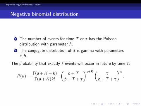
1 The number of events for time T or τ has the Poissondistribution with parameter λ.
2 The conjugate distribution of λ is gamma with parametersa, b.
The probability that exactly k events will occur in future by time τ:
P(k) =Γ(a+K + k)Γ(a+K )k !
b+ T
b+ T + τ
a+K τ
b+ T + τ
k.
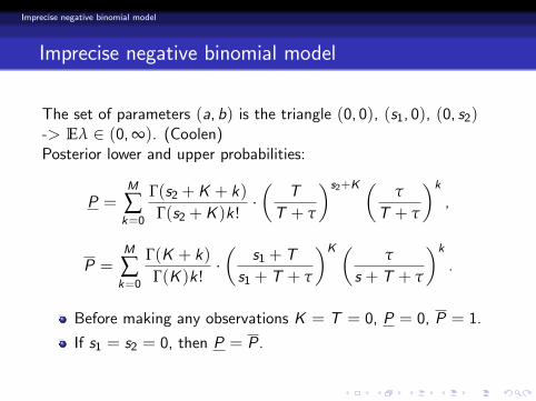
Imprecise negative binomial model
Imprecise negative binomial model
The set of parameters (a, b) is the triangle (0, 0), (s1, 0), (0, s2)-> Eλ 2 (0,∞). (Coolen)Posterior lower and upper probabilities:
P =M
∑k=0
Γ(s2 +K + k)Γ(s2 +K )k !
T
T + τ
s2+K τ
T + τ
k,
P =M
∑k=0
Γ(K + k)Γ(K )k !
s1 + T
s1 + T + τ
K τ
s + T + τ
k.
Before making any observations K = T = 0, P = 0, P = 1.
If s1 = s2 = 0, then P = P.

Imprecise negative binomial model
About two caution parameters
1 The lower bound E(s)i X is
E(s)i X = K
t
s + T
In fact, the parameter s here increases the time on the value s(hidden time).
2 The upper bound E(s)i X is
E(s)i X = (s +K )
t
T
In fact, the parameter s here increases the number of eventson the value s (hidden number of events).

Imprecise gamma-exponential model
Gamma-exponential distribution
1 Time to an event has the exponential distribution withparameter λ.
2 The conjugate distribution of λ is gamma with parametersa, b.
The probability of an event before T :
P(x < T ) =
b+ T
b+ T + x
a+n.

Imprecise gamma-exponential model
Imprecise gamma-exponential model
The set of parameters (a, b) is the triangle (0, 0), (s1, 0), (0, s2)-> Eλ 2 (0,∞).Posterior lower and upper probabilities:
P(x < T ) =
T
T + x
s2+n,
P(x < T ) =
s1 + T
s1 + T + x
n.
Before making any observations T = 0, n = 0, P = 0, P = 1.
If s1 = s2 = 0, then P = P.
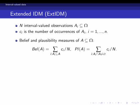
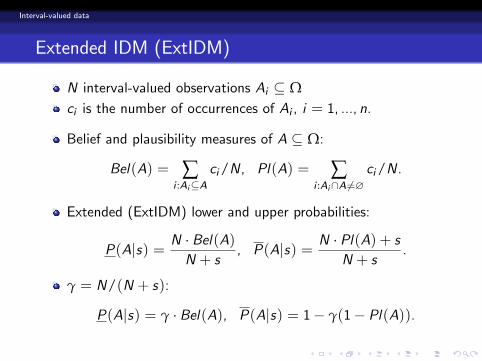
Interval-valued data
Extended IDM (ExtIDM)
N interval-valued observations Ai Ωci is the number of occurrences of Ai , i = 1, ..., n.
Belief and plausibility measures of A Ω:
Bel(A) = ∑i :AiA
ci/N, Pl(A) = ∑i :Ai\A 6=?
ci/N.
Extended (ExtIDM) lower and upper probabilities:
P(Ajs) = N Bel(A)N + s
, P(Ajs) = N Pl(A) + sN + s
.
γ = N/(N + s):
P(Ajs) = γ Bel(A), P(Ajs) = 1 γ(1 Pl(A)).
Interval-valued data
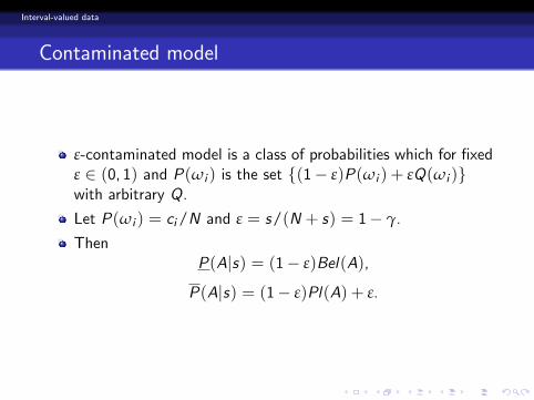
Contaminated model
ε-contaminated model is a class of probabilities which for xedε 2 (0, 1) and P(ωi ) is the set f(1 ε)P(ωi ) + εQ(ωi )gwith arbitrary Q.
Let P(ωi ) = ci/N and ε = s/(N + s) = 1 γ.
ThenP(Ajs) = (1 ε)Bel(A),
P(Ajs) = (1 ε)Pl(A) + ε.
Interval-valued data
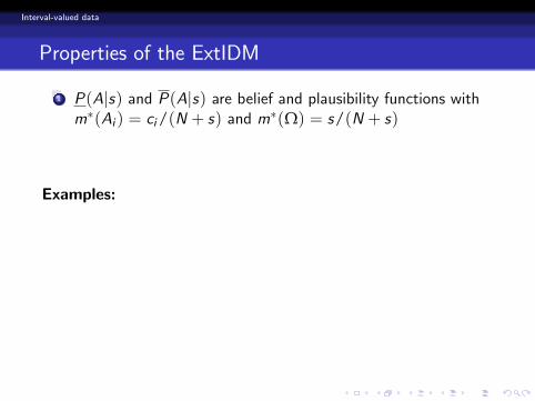
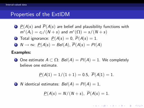
Properties of the ExtIDM
1 P(Ajs) and P(Ajs) are belief and plausibility functions withm(Ai ) = ci/(N + s) and m(Ω) = s/(N + s)
2 Total ignorance: P(Ajs) = 0, P(Ajs) = 1.3 N ! ∞: P(Ajs) = Bel(A), P(Ajs) = Pl(A)
Examples:
1 One estimate A Ω: Bel(A) = Pl(A) = 1. We completelybelieve one estimate.
P(Aj1) = 1/(1+ 1) = 0.5, P(Aj1) = 1.
2 N identical estimates: Bel(A) = Pl(A) = 1,
P(Ajs) = N/(N + s), P(Ajs) = 1.

Interval-valued data
Properties of the ExtIDM
1 P(Ajs) and P(Ajs) are belief and plausibility functions withm(Ai ) = ci/(N + s) and m(Ω) = s/(N + s)
2 Total ignorance: P(Ajs) = 0, P(Ajs) = 1.
3 N ! ∞: P(Ajs) = Bel(A), P(Ajs) = Pl(A)
Examples:
1 One estimate A Ω: Bel(A) = Pl(A) = 1. We completelybelieve one estimate.
P(Aj1) = 1/(1+ 1) = 0.5, P(Aj1) = 1.
2 N identical estimates: Bel(A) = Pl(A) = 1,
P(Ajs) = N/(N + s), P(Ajs) = 1.

Interval-valued data
Properties of the ExtIDM
1 P(Ajs) and P(Ajs) are belief and plausibility functions withm(Ai ) = ci/(N + s) and m(Ω) = s/(N + s)
2 Total ignorance: P(Ajs) = 0, P(Ajs) = 1.3 N ! ∞: P(Ajs) = Bel(A), P(Ajs) = Pl(A)
Examples:
1 One estimate A Ω: Bel(A) = Pl(A) = 1. We completelybelieve one estimate.
P(Aj1) = 1/(1+ 1) = 0.5, P(Aj1) = 1.
2 N identical estimates: Bel(A) = Pl(A) = 1,
P(Ajs) = N/(N + s), P(Ajs) = 1.

Interval-valued data
Properties of the ExtIDM
1 P(Ajs) and P(Ajs) are belief and plausibility functions withm(Ai ) = ci/(N + s) and m(Ω) = s/(N + s)
2 Total ignorance: P(Ajs) = 0, P(Ajs) = 1.3 N ! ∞: P(Ajs) = Bel(A), P(Ajs) = Pl(A)
Examples:
1 One estimate A Ω: Bel(A) = Pl(A) = 1. We completelybelieve one estimate.
P(Aj1) = 1/(1+ 1) = 0.5, P(Aj1) = 1.
2 N identical estimates: Bel(A) = Pl(A) = 1,
P(Ajs) = N/(N + s), P(Ajs) = 1.

Interval-valued data
Modied combination rule
Property 1 implies: extended BPAs are the discounted BPAs.
If s > 0, then 1K > 0 in Dempster's rule, where K representsbasic probability mass associated with con ict.
Modied Dempster's rule using extended BPAs works withcon icting evidence and con icting evidence can always becombined by means of the rule.

Applications
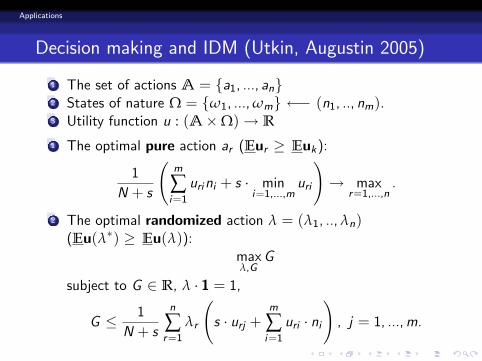
Decision making and IDM (Utkin, Augustin 2005)
1 The set of actions A = fa1, ..., ang2 States of nature Ω = fω1, ...,ωmg (n1, .., nm).3 Utility function u : (AΩ)! R
1 The optimal pure action ar (Eur Euk):
1
N + s
m
∑i=1
urini + s mini=1,...,m
uri
!! max
r=1,...,n.
2 The optimal randomized action λ = (λ1, ..,λn)(Eu(λ) Eu(λ)):
maxλ,G
G
subject to G 2 R, λ 1 = 1,
G 1
N + s
n
∑r=1
λr
s urj +
m
∑i=1
uri ni
!, j = 1, ...,m.
Applications
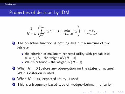
Properties of decision by IDM
1
N + s
m
∑i=1
urini + s mini=1,...,m
uri
!! max
r=1,...,n.
1 The objective function is nothing else but a mixture of twocriteria:
the criterion of maximum expected utility with probabilitiespi = ni/N - the weight N/(N + s)Wald's criterion - the weight s/(N + s)
2 When N = 0 (before any observation on the states of nature),Wald's criterion is used.
3 When N ! ∞, expected utility is used.4 This is a frequency-based type of HodgesLehmann criterion.

Applications
Decision making and ExtIDM (pure action)
1 N interval-valued observations Ai Ω2 ci is the number of occurrences of Ai , i = 1, ...,M.
1 The optimal pure action ar (Eur Euk):
1
N + s
s min
i=1,...,muri +
M
∑k=1
ck minωi2Ak
uri
!! max
r=1,...,n.
2 For comparison, Strat's approach (Strat 1990) (s = 0): 1
N
M
∑k=1
ck minωi2Ak
uri
!! max
r=1,...,n.

Applications
Decision making and ExtIDM (randomized action)
The optimal randomized action λ (Eu(λ) Eu(λ)):
1
N + s
s V0 +
M
∑k=1
ck Vk
!! max
λ,
subject to V0,Vi 2 R, λ 1 = 1,
Vi n
∑r=1
λrurj , i = 0, ...,M, j 2 Ji , J0 = f1, ...,mg.

Applications
Advantages of decisions with IDM (1)
Decision problem:
A = fa1, a2g,Ω = fω1,ω2g u =
ω1 ω2
a1 1000 1a2 0 0
There is only one judgment (M = 1): A1 = fx2g.
Standard belief functions (s = 0): a1 ( Eu1 = 1, Eu2 = 0(too optimistic).
IDM (s = 1): a2 ( Eu1 = (1000+ 1)/2 = 499.5,Eu2 = 0.

Applications
Advantages of decisions with IDM (1)
Decision problem:
A = fa1, a2g,Ω = fω1,ω2g u =
ω1 ω2
a1 1000 1a2 0 0
There is only one judgment (M = 1): A1 = fx2g.
Standard belief functions (s = 0): a1 ( Eu1 = 1, Eu2 = 0(too optimistic).
IDM (s = 1): a2 ( Eu1 = (1000+ 1)/2 = 499.5,Eu2 = 0.
Applications
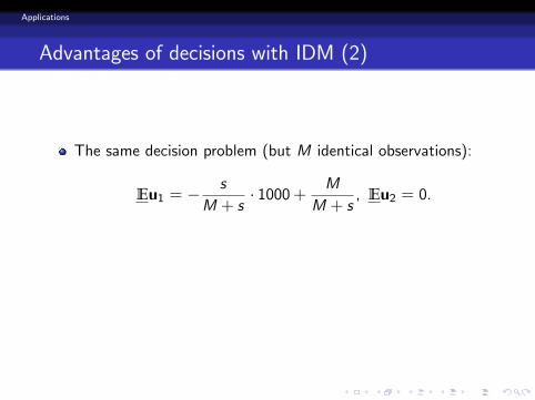
Advantages of decisions with IDM (2)
The same decision problem (but M identical observations):
Eu1 = s
M + s 1000+ M
M + s, Eu2 = 0.
s = 0: Eu1 = 1, Eu2 = 0 for all M = 1, 2, ....Our decision is the same irrespective of having 1 singleobservation or 10,000 identical observations.
s = 1: a1 is only superior when M > 1000.

Applications
Individual risk model of insurance (problem statement)
1 N identical insurance policies for time t.
2 The claim is denoted Xi = Ii yi , yi is the claim amount.
3 Each insurance premium is c .
4 The total premium is Π(t) = cN.5 The total amount of claims is R(t) = X1 + ...+ XN .
6 The probability that aggregate claims will be less than thepremium collected:
P = PrfΠ(t) R(t)g = PrfcN X1 + ...+ XNg.

Applications
Individual risk model of insurance (approaches)
If r.v. X1, ...,XN are independent, then P is the Cdf of numbers ofclaims:
P =M
∑k=0
p(k,w), M = dΠ(t)/ye = dcN/ye .
1 p(k,w) is the binomial distribution with w = q:
P =M
∑k=0
N
k
qk(1 q)Nk .
2 p(k,w) is the Poisson distribution with w = λ:
P =M
∑k=0
(λt)k exp(λt)
k !.

Applications
If numbers of claims are binomially distributed
Imprecise beta-binomial modelPosterior lower and upper probabilities:
P =M
∑k=0
N
k
B(s + k +K ,N +N k K )
B(s +K ,N K ) ,
P =M
∑k=0
N
k
B(k +K , s +N +N k K )
B(K , s +N K ) .

Applications
If numbers of claims have the Poisson distribution
Imprecise negative binomial modelPosterior lower and upper probabilities:
P =M
∑k=0
Γ(s +K + k)Γ(s +K )k !
T
T + τ
s+K τ
T + τ
k,
P =M
∑k=0
Γ(K + k)Γ(K )k !
s + T
s + T + τ
K τ
s + T + τ
k.
Applications
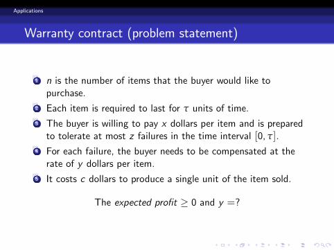
Warranty contract (problem statement)
1 n is the number of items that the buyer would like topurchase.
2 Each item is required to last for τ units of time.
3 The buyer is willing to pay x dollars per item and is preparedto tolerate at most z failures in the time interval [0, τ].
4 For each failure, the buyer needs to be compensated at therate of y dollars per item.
5 It costs c dollars to produce a single unit of the item sold.
The expected prot 0 and y =?

Applications
Warranty contract (approaches)
The probability of i failures in the time interval [0, τ] with theparameter λ: p(i jλ)The expected prot: EλB=n(x c) y ∑n
i=1 i p(i jλ)By using imprecise negative binomial model, we have
EB = n(x c) yn
∑k=1
Γ(s +K + k)Γ(s +K )(k 1)!
T
T + τ
s+K τ
T + τ
k.
EB = n(x c) yn
∑k=1
Γ(K + k)Γ(K )(k 1)!
s + T
s + T + τ
K τ
s + T + τ
k.

Applications
Warranty contract (numerical results)
y = y : EB(y) 0, y = y : EB(y) 0
2 4 6 8
10000
20000
30000
40000
T
y
Lower and upper bounds for y by s = 1

Expected Utilities by Continuous Probability Distributions
Problem statement
Given F (x) F (x) F (x), 8x 2 R
The lower and upper expected utilities of h(X ) :
Eh = infFFF
ZRh(x)dF (x), Eh = sup
FFF
ZRh(x)dF (x).
Approximate solution:
Eh = infN
∑k=1
h(xk)zk , Eh = sup
N
∑k=1
h(xk)zk ,
subject to
zk 0, i = 1, ...,N,N
∑k=1
zk = 1,
i
∑k=1
zk F (xi ),i
∑k=1
zk F (xi ), i = 1, ...,N.

Expected Utilities
Monotone utility function
1 If the function h is non-decreasing in R, then
Eh =Z
Rh(x)dF (x), Eh =
ZRh(x)dF (x).
2 If the function h is non-increasing in R, then
Eh =Z
Rh(x)dF (x), Eh =
ZRh(x)dF (x).
Expected Utilities
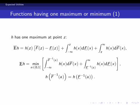
Functions having one maximum or minimum (1)
h has one maximum at point z :
Eh = h(z)F (z) F (z)
+Z z
∞h(x)dF (x) +
Z ∞
zh(x)dF (x),
Eh = minα2[0,1]
"Z F1(α)
∞h(x)dF (x) +
Z ∞
F1(α)h(x)dF (x)
#,
hF1(α)= h
F1(α)
.
Expected Utilities
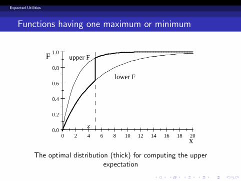
Functions having one maximum or minimum
0 2 4 6 8 10 12 14 16 18 200.0
0.2
0.4
0.6
0.8
1.0
x
F
z
lower F
upper F
The optimal distribution (thick) for computing the upperexpectation

Expected Utilities
Functions having one maximum or minimum
0 2 4 6 8 10 12 14 16 18 200.0
0.2
0.4
0.6
0.8
1.0
x
F
z
α
lower F
upper F
The optimal distribution (thick) for computing the lowerexpectation
Expected Utilities
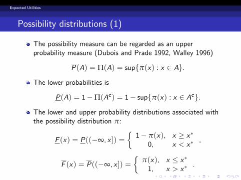
Possibility distributions (1)
The possibility measure can be regarded as an upperprobability measure (Dubois and Prade 1992, Walley 1996)
P(A) = Π(A) = supfπ(x) : x 2 Ag.
The lower probabilities is
P(A) = 1Π(Ac) = 1 supfπ(x) : x 2 Acg.
The lower and upper probability distributions associated withthe possibility distribution π:
F (x) = P((∞, x ]) =1 π(x), x x
0, x < x,
F (x) = P((∞, x ]) =
π(x), x x1, x > x
.
Expected Utilities
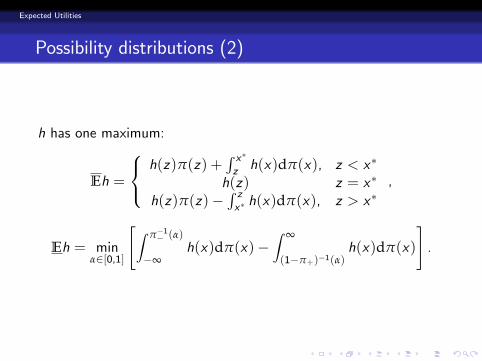
Possibility distributions (2)
h has one maximum:
Eh =
8<: h(z)π(z) +R xz h(x)dπ(x), z < x
h(z) z = x
h(z)π(z)R zx h(x)dπ(x), z > x
,
Eh = minα2[0,1]
"Z π1 (α)
∞h(x)dπ(x)
Z ∞
(1π+)1(α)h(x)dπ(x)
#.

Expected Utilities
Possibility distributions of the triangular form
π(x) =
8<:(x a1)/(x a1), a1 < x x(a2 x)/(a2 x), x < x a2
0, otherwise.
Eh =1
x a1
(z a1)h(z) +
Z x
zh(x)dx
,
Eh =1
x a1
Z α(xa1)+a1
a1h(x)dx+
1
a2 xZ a2
α(a2x)+xh(x)dx ,
α( h (α (x a1) + a1) = h (α (a2 x) + x) .

Expected Utilities
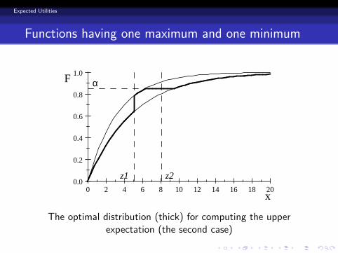
Functions having one maximum and one minimum
0 2 4 6 8 10 12 14 16 18 200.0
0.2
0.4
0.6
0.8
1.0
x
F
z1 z2
α
The optimal distribution (thick) for computing the upperexpectation (the rst case)
Expected Utilities
Functions having one maximum and one minimum
0 2 4 6 8 10 12 14 16 18 200.0
0.2
0.4
0.6
0.8
1.0
x
F
z1 z2
α
The optimal distribution (thick) for computing the upperexpectation (the second case)
Expected Utilities
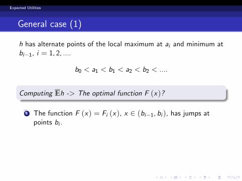
General case (1)
h has alternate points of the local maximum at ai and minimum atbi1, i = 1, 2, ....
b0 < a1 < b1 < a2 < b2 < ....
Computing Eh -> The optimal function F (x)?
1 The function F (x) = Fi (x), x 2 (bi1, bi ), has jumps atpoints bi .
2 The size of the i-th jump is
minF (bi ) , αi+1
max (F (bi ) , αi ) .
3 Between jumps ...
Expected Utilities
General case (1)
h has alternate points of the local maximum at ai and minimum atbi1, i = 1, 2, ....
b0 < a1 < b1 < a2 < b2 < ....
Computing Eh -> The optimal function F (x)?
1 The function F (x) = Fi (x), x 2 (bi1, bi ), has jumps atpoints bi .
2 The size of the i-th jump is
minF (bi ) , αi+1
max (F (bi ) , αi ) .
3 Between jumps ...

Expected Utilities
General case (2)
Between jumps
Fi (x) =
8<:F (x) , x < a0
α, a0 x a00F (x) , a00 < x
,
where α is the root of the equation
hmax
F1(α) , bi1
= h
min
F1 (α) , bi
in interval
F (ai ) ,F (ai )
,
a0 = maxF1(α) , bi1
, a00 = min
F1 (α) , bi
.

Expected Utilities
Questions
?


![04.03 Imprecise Task Schedule Optimization [I].pdf](https://static.fdocuments.us/doc/165x107/577cc0951a28aba7119090f6/0403-imprecise-task-schedule-optimization-ipdf.jpg)


