Implicit surface tension model for stimulation of ... · Implicit surface tension model for...

Implicit surface tension model for stimulation ofinterfacial flows

Vinh The Nguyen

University of Massachusetts Dartmouth

March 3rd, 2011

Implicitmodeling

Nguyen

About my project

Project Advisor

• Dr. Mehdi Raessi

• Department of Mechanical Engineering

Project Objective

• To study implicit modeling of surface tension.

• To generate faster and better model that produce nospurious currents and has larger time step restriction.

2 / 23

Implicitmodeling

Nguyen

Introduction

• What is interfacial flow?

• What are the applications?

3 / 23

Applications of interfacial flow

Implicitmodeling

Nguyen

Modeling of interfacial flow

• To accurately model the interfacial flow is challengingbecause:

• The discontinuity of fluid properties (such as density).

• The interfacial boundary condition (surface tension).

5 / 23

Implicitmodeling

Nguyen

Modeling of surface tension in interfacial flow

Currently there are two main interfacial flow models

• Explicit:Precise but has high computational cost due to small timestep restriction.

• Implicit:Lower computational cost than explicit due to highertime-step restriction.Draw backs: appearing of nonphysical velocities (spuriouscurrent)Common flow solver: Continuum surface force (CSF)

6 / 23

Implicitmodeling

Nguyen

Method used

CSF method

• The implicit model studied in this project is based onContinuum Surface Force method

• This method was first proposed by Brackbill et al. 1991

Drawbacks:

• This method generates unphysical velocities (spuriouscurrents)

• The spurious current is caused by:

• Imbalance of the surface tension and pressure gradient.

• Error in computing the curvature. (this project)

7 / 23

Implicitmodeling

Nguyen

(Francois et al. 2007)The pressure drop across the interface:

∆p = p2 − p1 = σk (1)

σ is the surface tension coefficientk is the mean curvature

k =1RI

+1RII

(2)

δ is the delta function represent interface (Raessi et al. 2008)

8 / 23

Implicitmodeling

Nguyen

My task

Tasks:

• Study the CSF model

• Study the stability of the model (CFL condition) astime-step increases using different curvature solvingmethod: Level set (LS) and Advecting Normal

• Compare the results with exact curvature.

Challenges:

• To get used to the code and understand what’s thefunction of each parts requires lots of trials errors.

• To manipulate it to do what I want also requires lots oftrials and errors.

9 / 23

Implicitmodeling

Nguyen

CFL number/ CFL condition

• The Courant-Friedrichs-Lewy condition (CFL condition) isa necessary condition for convergence while solving partialdifferential equations numerically.

CFL =u.∆t∆x

≤ C (3)

C= 1

10 / 23

Implicitmodeling

Nguyen

Level Set methodFor a 2D interface between two fluids, depicted in Fig. 1a, the discretized VOF function representing fluid 1

is shown in Fig. 1b. As can be seen, the volume fractions vary sharply from zero to one across the interface.This discontinuous behavior makes it di!cult to accurately evaluate the first and second derivatives of f, whichleads to inaccurate interface normals and curvatures. Smoothing the f field prior to evaluating $f improves thevalues [12]. We assess the accuracy of n̂ and j calculated from f in Section 2.3. But first, we briefly present theLS method, which is known to yield more accurate normals and curvatures.

2.2. Level set method

In the LS method, the interface is represented by a smooth function / – called the LS function; for adomain X, / is defined [15] as a signed distance to the boundary (interface) oX

j/!~x"j # min!j~x$ ~xI j" for all ~xI 2 oX !6"

implying that /!~x" # 0 on oX. Choosing / to be positive inside X, we then have

/!~x" #> 0; ~x 2 X

0; ~x 2 oX< 0; ~x 62 X

8><

>:!7"

For the 2D interface depicted in Fig. 1a, the discretized LS function, defined at the center of each cell, is shownin Fig. 1c.

The unit normal vector and curvature at any point on the interface are calculated from / by

n̂ # r/jr/j !8"

and

j # $r % r/jr/j

! "!9"

Since / is smooth and continuous across the interface (see Fig. 1c), $/ can be calculated accurately.In the LS method, the motion of the interface is defined by the following advection equation:

o/ot

&~u %r/ # 0 !10"

When / is advected, the / = 0 contour moves at the correct interface velocity; however, contours of / 6# 0 donot necessarily remain distance functions. This can result in an irregular / field that in turn leads to problems

Fig. 1. (a) A 2D interface between fluids 1 and 2, (b) the discretized VOF function representing fluid 1 and (c) the level set functionrepresenting distance to the interface.

776 M. Raessi et al. / Journal of Computational Physics 226 (2007) 774–797

(Raessi et al. 2007)

11 / 23

Implicitmodeling

Nguyen

Level Set method

For a 2D interface between two fluids, depicted in Fig. 1a, the discretized VOF function representing fluid 1is shown in Fig. 1b. As can be seen, the volume fractions vary sharply from zero to one across the interface.This discontinuous behavior makes it di!cult to accurately evaluate the first and second derivatives of f, whichleads to inaccurate interface normals and curvatures. Smoothing the f field prior to evaluating $f improves thevalues [12]. We assess the accuracy of n̂ and j calculated from f in Section 2.3. But first, we briefly present theLS method, which is known to yield more accurate normals and curvatures.

2.2. Level set method

In the LS method, the interface is represented by a smooth function / – called the LS function; for adomain X, / is defined [15] as a signed distance to the boundary (interface) oX

j/!~x"j # min!j~x$ ~xI j" for all ~xI 2 oX !6"

implying that /!~x" # 0 on oX. Choosing / to be positive inside X, we then have

/!~x" #> 0; ~x 2 X

0; ~x 2 oX< 0; ~x 62 X

8><

>:!7"

For the 2D interface depicted in Fig. 1a, the discretized LS function, defined at the center of each cell, is shownin Fig. 1c.

The unit normal vector and curvature at any point on the interface are calculated from / by

n̂ # r/jr/j !8"

and

j # $r % r/jr/j

! "!9"

Since / is smooth and continuous across the interface (see Fig. 1c), $/ can be calculated accurately.In the LS method, the motion of the interface is defined by the following advection equation:

o/ot

&~u %r/ # 0 !10"

When / is advected, the / = 0 contour moves at the correct interface velocity; however, contours of / 6# 0 donot necessarily remain distance functions. This can result in an irregular / field that in turn leads to problems

Fig. 1. (a) A 2D interface between fluids 1 and 2, (b) the discretized VOF function representing fluid 1 and (c) the level set functionrepresenting distance to the interface.



12 / 23

Implicitmodeling

Nguyen

Advecting Normal method

Note that the order of accuracy of the CLSVOF method used in this work is consistent [27] with the accu-racy of a similar model developed by Sussman and Puckett [24]. Although n̂ and j calculated from the LSfunction are much more accurate than those calculated from the VOF function, neither approach yields con-verging curvatures.

Finally, it should be noted that these results only apply to the LS function in a CLSVOF context. Othermethods for constructing a distance function (discussed in Section 2.2) may yield converging curvatures, evenwith second-order accuracy; however, such methods will fail to exactly conserve mass.

The objective, then, of this work was to devise a method to calculate second-order accurate, or at least con-verging, curvatures. Such a method is presented next, in which interface normals are advected with the flow,and curvatures are calculated directly from the advected normals.

3. Advecting normals: a new method for calculating interface normals and curvatures

3.1. Mathematical fundamentals

As reviewed earlier, the evolution of the LS function is governed by Eq. (10)

o/ot

!~u "r/ # 0

Defining ~N # r/ as the vector normal to the contours of /, the above equation can be rewritten as

o/ot

!~u " ~N # 0 $14%

Taking the gradient of Eq. (14), we obtain

o~Not

!r ~u " ~N! "

# 0 $15%

Eq. (15) is the advection equation for normals. In 2D Cartesian coordinates, Eq. (15) results in the followingequations:

oNx

ot! oox

$uNx ! vNy% # 0 $16%

and

oNy

ot! ooy

$uNx ! vNy% # 0 $17%

Next, consider the following lemma [28]:Let un #~u "r/ be the normal velocity of each level set, and set /$~x; 0% to be the signed distance function. Then

/ remains a signed distance function if and only if run "r/ # 0.The condition run "r/ # 0 can be also expressed as

r$~u " ~N% " ~N # 0 $18%

Note that jr/j #j ~N j # 1. Now, from Eq. (15) we obtain

o~Not

" ~N !r$~u " ~N% " ~N # 0 $19%

or

1

2

oot$j~N j2% !r$~u " ~N% " ~N # 0 $20%


Note that the order of accuracy of the CLSVOF method used in this work is consistent [27] with the accu-racy of a similar model developed by Sussman and Puckett [24]. Although n̂ and j calculated from the LSfunction are much more accurate than those calculated from the VOF function, neither approach yields con-verging curvatures.

Finally, it should be noted that these results only apply to the LS function in a CLSVOF context. Othermethods for constructing a distance function (discussed in Section 2.2) may yield converging curvatures, evenwith second-order accuracy; however, such methods will fail to exactly conserve mass.

The objective, then, of this work was to devise a method to calculate second-order accurate, or at least con-verging, curvatures. Such a method is presented next, in which interface normals are advected with the flow,and curvatures are calculated directly from the advected normals.

3. Advecting normals: a new method for calculating interface normals and curvatures

3.1. Mathematical fundamentals

As reviewed earlier, the evolution of the LS function is governed by Eq. (10)

o/ot

!~u "r/ # 0

Defining ~N # r/ as the vector normal to the contours of /, the above equation can be rewritten as

o/ot

!~u " ~N # 0 $14%

Taking the gradient of Eq. (14), we obtain

o~Not

!r ~u " ~N! "

# 0 $15%

Eq. (15) is the advection equation for normals. In 2D Cartesian coordinates, Eq. (15) results in the followingequations:

oNx

ot! oox

$uNx ! vNy% # 0 $16%

and

oNy

ot! ooy

$uNx ! vNy% # 0 $17%

Next, consider the following lemma [28]:Let un #~u "r/ be the normal velocity of each level set, and set /$~x; 0% to be the signed distance function. Then

/ remains a signed distance function if and only if run "r/ # 0.The condition run "r/ # 0 can be also expressed as

r$~u " ~N% " ~N # 0 $18%

Note that jr/j #j ~N j # 1. Now, from Eq. (15) we obtain

o~Not

" ~N !r$~u " ~N% " ~N # 0 $19%

or

1

2

oot$j~N j2% !r$~u " ~N% " ~N # 0 $20%



13 / 23

Implicitmodeling

Nguyen

Case study: Static drop

• Static water drop in zero gravity.

• ρ1 = ρ2 = 103Kg/m3

• µ1 = µ2 = 0.05• g = 0• Surface tension time-step restriction ∆tST = 0.03


14 / 23

Implicitmodeling

Nguyen

What I did

15 / 23

Implicitmodeling

Nguyen

Results - Level Set method vs. Exact Curvature

0 10 20 30 40 50 60 70 80 900

1

2

3

4

5

6

7

8x 10

!4 CFL vs. t for COMPUTED CURVATURE

CF

L

t (s)

CFL @dt =0.015s

CFL @dt =0.03s

CFL @dt =0.06s

Student Version of MATLAB

• Level set

0 10 20 30 40 50 60 70 80 900

1

2

3

4

5

6

7x 10

!8 CFL vs. t for Exact CURVATURE

CF

L

t (s)

CFL @dt =0.015s

CFL @dt =0.03s

CFL @dt=0.06s

CFL @dt=0.12s


• Exact curvatureThe timestep was increase as : ∆t = 0.5, 2, 4∆tST

16 / 23

Implicitmodeling

Nguyen

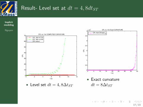
Result- Level set at dt = 4, 8dtST

0 2 4 6 8 10 120

10

20

30

40

50

60

70CFL vs. t for COMPUTED CURVATURE

CF

L

t (s)

CFL @dt =0.12s

CFL @dt =0.24s

CFL limit=1


• Level set dt = 4, 8∆tST

0 5 10 15 20 25 30 35 400

0.5

1

1.5

2

2.5

3

3.5

4x 10

7 CFL vs. t for Exact CURVATURE

CF

L

t (s)

CFL @dt =8*delta tST


• Exact curvaturedt = 8∆tST

17 / 23

Implicitmodeling

Nguyen

Result- Level set vs. Exact Curvature for maximumtimestep

0 10 20 30 40 50 60 70 80 900

0.5

1

1.5

2

2.5

3

3.5

4

4.5

Time s

CF

L

CFL vs. Time for Computed Curvature

CFL @dt =0.096s

CFL @dt=0.095s


• Level setdt = 3.167, 3.2∆tST

0 10 20 30 40 50 60 70 80 900

0.2

0.4

0.6

0.8

1

1.2

1.4

Time s

CF

L

CFL vs. Time for Exact Curvature

CFL @dt=0.21s=7dtST

CFL@dt = 0.2s=6.67dtST

CFL limit


• Exact curvaturedt = 6.67, 7∆tST

18 / 23

Implicitmodeling

Nguyen

Result- Level set vs Advecting Normal

0 10 20 30 40 50 60 70 80 900

0.5

1

1.5

2

2.5

3

3.5

4

4.5

Time s

CF

LCFL vs. Time for Exact Curvature

CFL @dt=0.095s AN

CFL @dt=0.096s AN

CFL @dt=0.095s LS

CFL @dt=0.096s LS


19 / 23

Implicitmodeling

Nguyen

Question

20 / 23

Implicitmodeling

Nguyen

Conclusion

Proved:

• To accurately compute the curvature is crucial and it canincrease the stability of the solution for implicit model

21 / 23

Implicitmodeling

Nguyen

Future Research

• Continue to study the implicit models.

• Starting with the simulation.

22 / 23

Implicitmodeling

Nguyen

References

Mehdi RaessiModeling surface tension-dominant, large density ratio, two-phaseflow, 2008University of Toronto

J. U. BRACKBILL, D. B. KOTHE, AND C. ZEMACHA Continuum Method for Modeling Surface tensionTheoretical Division, Los Alamos National Laboratory, Los Alamos,New Mexico,87545, July 1991.

M. Raessi, J. Mostaghimi, M. BussmannAdvecting normal vectors: A new method for calculating interfacenormals and curvatures when modeling two-phase ßowsDepartment of Mechanical and Industrial Engineering, University ofToronto, Canada, April 28, 2007.

Marianne M. Francois, James M. Sicilian, CCS-2; Douglas B. KotheModeling Interfacial Surface Tension in Fluid FlowOak Ridge National Laboratory, 2007

23 / 23

Implicit surface tension model for stimulation of ... · Implicit surface tension model for...

Documents

Transcript of Implicit surface tension model for stimulation of ... · Implicit surface tension model for...