Implicit Generation and Generalization withEnergy-Based Models

Yilun DuOpenAI

Igor MordatchOpenAI

Abstract

Energy based models (EBMs) are attractive due to their generality and simplicityin likelihood modeling, but have been traditionally difficult to train. We presenttechniques to scale EBM training through a MCMC framework on modern ar-chitectures. We show that MCMC on EBMs generates realistic image sampleson CIFAR10 that are more coherent than state of the art likelihood models andcomparable to GANs without exhibiting mode collapse, and on time series dataare significantly better than identical feedforward models. We further show thatEBMs are able to achieve better out of distribution generalization than other stateof the art generative models (such as assigning high likelihood to CIFAR10 imagesthan SVHN images), and are able to additively combine at test time to generatecombinations of several different latents.

1 Introduction

Two fundamental problems with deep learning are data efficiency and out of distribution general-ization. Generative models capture world knowledge and enable faster learning. At the same time,generative modeling helps prevents catastrophical failure in out of distribution cases.

Generative modeling has seen a flux of interest. Many approaches reply on directly maximizing thelikelihood. Modeling a correlated high dimensional data distribution is difficult. Auto-regressivemodels [Van Oord et al., 2016, Graves, 2013] solve this by completely factorizing the underlyingdistribution, but such an approach leads to compounding error and a loss of underlying structural in-formation. Other approaches such as the variational auto-encoder [Kingma and Welling, 2014] or flowbased models [Dinh et al., 2014, Kingma and Dhariwal, 2018] rely on a factorized prior distributionto simplify likelihood estimation. Flow models require invertible Jacobian transformations, whichcan limit model capacity and have difficulty fitting discontinuous data. Such approximations haveprevented likelihood models from generating high quality images in diverse domains. In contrast,approaches based off generative adversarial networks [Goodfellow et al., 2014] put no constraints onlatent space and have generated high quality images but do not cover the entire data distribution.

Energy based models (EBMs) are flexible likelihood model with no latent constraints [LeCun et al.,2006]. EBMs received attention in the past [Hinton et al., 2012, Dayan et al., 1995] but have not seenwide adoption due to an expensive negative sampling phase. We propose methods to scale up EBMsto modern day architectures. We find that these EBMs are able to generate significantly better samplesthan other likelihood models and are competitive with GANs on CIFAR10 (inception score) in imagequality and better than corresponding feedforward networks in time series modeling. Through severalimage completion experiments and likelihood evaluation, we find that the sample quality does notcome at the expense of mode collapse. Furthermore, we show that EBMs generalize well, beingsignificantly better at out of distribution generalization than other state of the art likelihood models,such as being able to assign higher log likelihood to CIFAR10 test images than SVHN images, whilesimultaneously being able to effectively generate samples when jointly conditioned on independentconditional EBMs for seperate latents.

Third workshop on Bayesian Deep Learning (NeurIPS 2018), Montréal, Canada.

2 Related WorkEnergy based models have seen large amounts of attention in the past [LeCun et al., 2006, Hintonet al., 2012]. Previous methods have also relied on MCMC training to sample from the partitionfunction, but have primarily relied on Gibb’s Sampling on older architectures [Nair and Hinton,2010]. We instead use Langevin Dynamics (also used in [Mnih and Hinton]) or MPPI([Williamset al., 2017]) to more efficiently sample negative samples on modern architectures.

We show a connection of energy based training to GANS which has also been shown in [Finn et al.,2016, Zhao et al., 2016, Kim and Bengio, 2016]. Finn et al. [2016] show a direct connection betweentraining a GAN and energy functions, using a separate proposal distribution q(x) to estimate thepartition function. Zhao et al. [2016], Kim and Bengio [2016] and many related works use adversarialtraining on a separate q(x) to provide fast estimation of the partition function. Our work is separatefrom these models as we use a MCMC approximation of the original function to estimate the partitionfunction and use this MCMC approximation as our generator. Since our "generator" is then dependenton our original function, this allows the generator to adapt implicitly while only training our energyfunction (discriminator). This then removes the need to train generator, which combined with thefact the model itself has modes of probability at all training data points, reduces the likelihood ofmode collapse. Our derivation for EBMs further shows that maximizing likelihood under an optimal"generator" corresponds exactly to the Wassterstein GAN criterion [Arjovsky et al., 2017].

3 Scaling EBM TrainingIn the section, we formulate our method for training EBMs. We outline our likelihood objective andsampling distributions. We then detail architectural changes and sample tricks allowing better overallsampling. Finally, we provide our overall loss and show a connection GAN based training.

3.1 Likelihood ObjectiveOur overall algorithm for training algorithm for EBMs follows the contrastive divergence algorithm[Hinton, 2002]. Given an energy function E(x; θ) ∈ R , represented as a a neural network ∗, wemodel the probability distribution as p(x) through the Gibb’s distribution.

p(x) =e−E(x;θ)

Z(θ); Z(θ) =

∫e−E(y;θ)dy

Given data distribution pd(x), we seek to minimize negative likelihood given by

Ex∼pd(x)[E(x; θ) + log(

∫e−E(y;θ)dy)

]= Ex∼pd(x)

[E(x; θ) + log(Ey∼q(x)[e−E(y;θ)/q(y)])

](1)

where q(x) is a proposal distribution which we choose to be a finite step MCMC approximation ofp(x). Evaluating the exact likelihood q(y) is difficult to calculate. We choose to use one of either twoapproximations: either that q(y) has uniform probability or if q(y) matches the energy distributionp(y). If we assume that all q(y) are equal, we have an approximate negative log likelihood objectiveof

minθ

Ex∼pd(x)[E(x; θ) + log(Ey∼q(x)[e−E(y;θ)])

](2)

Alternatively, if we assume that q(y) = p(y) then we obtain the exact negative log likelihoodobjective below from Equation 1 (derivation in Section 8.1).

minθ

Ex∼pd(x)[E(x; θ)− Ey∼q(x)[E(y; θ)]

](3)

Empirically, we find that q(y) appears to have almost equal probability distribution to pd(x) (Figure 1),indicating that its likely that q(y) = p(y), indicating a preference of Equation 3. However, duringtraining, we found that empirically Equation 3 was slightly less stable than Equation 2, so we chooseto use Equation 2 for our training procedures.∗We use residual networks [He et al., 2015] with zero initialization [Anonymous, 2019b] for images. For

time series prediction we use a combination of fully connected, self-attention and 1D convolutions layers (seeappendix)

2

3.2 Proposal Distributions

To we use a proposal distribution q(x) to estimate samples for the likelihood objective. In contrastto recent works, our proposal distributions are MCMC approximations of the original distributioninstead of a separate network. We either use Langevin dynamics (LD) [Welling and Teh, 2011]

x̃q = x̃k, x̃k = x̃k−1 − λ(∇xk−1E(x̃k−1) + ωk; θ), ω ∼ N(0, σ) (4)

or MPPI based MCMC sampling [Williams et al., 2017]

x̃k =∑i

wixki , xki ∼ N(0, σ) + xk−1, wi =

(e−E(xki ;θ)∑j e−E(xji ;θ)

)(5)

Figure 1: Relative energy of points sampled fromq(x) compared to CIFAR10 train data points. Wefind that q(x) exhibits a relatively similar distribu-tion to pd(x).

where for stability, we further clip gradients inLD sampling. We find that either MCMC pro-posals lead to good training performance, withLD scaling better on high dimensional data, butMPPI sampling working better on lower dimen-sional data. The gradient descent direction givenby an energy function in LD allows quick modegeneration, but may also make it difficult to findall nearby modes, which MPPI sampling allows.We demonstrate that both methods perform wellon time series data but for images, only LD wasviable.

At the start of training, we initialize MCMCchains with uniform random noise. To improvemixing of MCMC chains, as training progresses,we maintain a replay buffer of past generatedsamples, occasionally re-initializing certain sam-ples with random noise. This is similar to PCDin [Tieleman, 2008], but a replay buffer has theadded benefit of discouraging models from ex-

hibiting cyclical behavior. Furthermore, a replay buffer encourages models to not have spuriousmodes at all stages of sampling, and we found it crucial for sampled images to be reasonable, even ifsampling procedure significantly longer than during training.

3.3 Model Constraints

Arbitrary energy models can have sharp changes in gradients that make sampling with LD verydifficult. We find that simply constraining the Lipschitz constant remove many of these problems andallow most architectures blocks (residual, self attention,) to be at sample-able and thus trainable inenergy based models, as long as activations were kept piecewise linear without activation normal-ization. To constrain the Lipschitz constant, we follow the method of [Miyato et al., 2018] and addspectral normalization to all layers of the model.

Constraining the Lipschitz constant in models can significantly reduce the capacity of models andthere may exist blocks that are not easily samplable even with spectral normalization. A more generalsolution we found was to then add an additional loss to minimize KL distance between proposaldistribution and the original distribution (with the drawback of computational expense).

Specifically, we minimize the KL objective

minθKL(q(x; θ), p(x; stop_gradient(θ))) = min

θ−Exi∼q(x;θ)[E(xi; stop_gradient(θ))] (6)

. We note that both MCMC sampling distributions are differentiable, allowing us to change ourmodel’s landscape to be more samplable. We choose to ignore the first entropy term of the KLdivergence, as it is difficult to evaluate the likelihood of q(x). Methods such as [Liu et al., 2017] maybe helpful in simultaneously minimizing both terms.

3

In our tasks, we found that constrained Lipschitz residual networks were sufficiently expressive tomodel images. In cases of particle dynamics, we found the Lipschitz constant constraint overlyrestrictive and chose to add the above loss to impose samplebility.

3.4 Loss Functions

For training EBMs we use three different loss functions, LML, a maximum likelihood loss describedin Section 3.1, LKL, an optional sampling loss described in Section 3.3 and a regularization loss LReg.Our overall loss function is given by

Ltotal = LML + LKL + LReg

For LML we approximate Equation 2 over N points, where x−i and sampled from proposal distributionq(x; θ) and x+i are real data points to obtain the following loss.

LML =1

N

N∑i=0

E(x+i ; θ) + log(

N∑i=0

e−E(x−i ;θ)) (7)

In practice, we found that gradient of the log termN∑i=0

( e−Eθ(x−i

)∑i e

−Eθ(x−i

))E(x−i ) to be numerically unstable

due to close to zero denominators. Therefore, we rewrite our objective in an equivalent form whichremoves this issue.

LML =1

N

N∑i=0

Eθ(x+i )−

N∑i=0

−stop_gradient

(e−Eθ(x

−i )∑

i e−Eθ(x−

i ) + ε

)E(x−i ) (8)

When using a sampling loss (only on time series data), we approximate Equation 6 over N points toget

LKL =1

N

∑xi∼q(x)

Estop_gradient(θ)(q(xi)) (9)

Finally, we add a regularization loss to prevent energy explosion during training, as above losses onlyenforce relative energy difference between points and not absolute energy magnitude.

LReg =1

N

∑i

Eθ(x+i )

2 + Eθ(x−i )

2 (10)

We include a detail of our algorithm in Algorithm 1

3.5 Relationship to GAN training

We note that our likelihood objective is similar to GAN training objective training, where the generatorG(x) is our MCMC proposal distribution q(x) and the discriminator is the energy function p(x). Infact, when setting N = 1 in Equation 7 or assuming q(x) = p(x) Equation 3, we precisely obtain theWasserstein objective [Arjovsky et al., 2017]. Furthermore, in cases where proposal distribution is LDsampling on residual network based EBM, we note each step of sampling is operationally equivalentto a forward pass through a generator, since the gradient of a convolution is a deconvolution.

However an important difference between our likelihood training and GAN based training is thatour "generator" is implicitly a function of our "discriminator" (and in the infinite limit of numberof the steps the "discriminator"). As a result, the "generator" is able to co-adapt with training of thediscriminator and there is no need to explicitly train the "generator". This reduces the likelihood ofover-fitting of the "generator" and makes it exhibit the same modes that a discriminator exhibits.

This connections may explain one reason in which EBMs are able to sharper samples than otherlikelihood models. However, we note that unlike in GANs, our generation procedure doesn’t appearto exhibit significant mode collapse as seen in Figure 4.

4

4 Images ModelingWe measure EBM’s ability to model complex distribution on both class-conditional and unconditionalCIFAR10 datasets. Our model is based on the ResNet architecture (using conditional gains and biasesper class) with details in Section 8.5. Our models have around 7-20 million parameters, comparativelysmaller than other state of the art models. We preprocess images to be between 0 and 1 with details inSection 8.6. We evaluate EBMs ability to generate images, show that it constructs a good likelihoodmodel of the underlying distribution, measure representation learning, and show that exhibits goodout of distribution generalization

(a) GLOW [Kingma and Dhari-wal, 2018] samples

(b) UnconditionalEBM samples

(c) Historical ensemble(10) EBMunconditional samples

Figure 2: Illustrations of image generation from GLOW as compared to our EBM models. Ourmodels are able to more accurately generate objects.

(a) conditional CIFAR10 EBM samples

Model Inception Score

Unconditional CIFAR10

PixelCNN 4.60DCGAN 6.40Ours (single) 6.43Ours (10 historical ensemble) 6.79Conditional CIFAR10

Improved GAN 8.09Ours 8.52Spectral Normalization GAN 8.59

(b) Table of Inception Scores

4.1 Image Generation

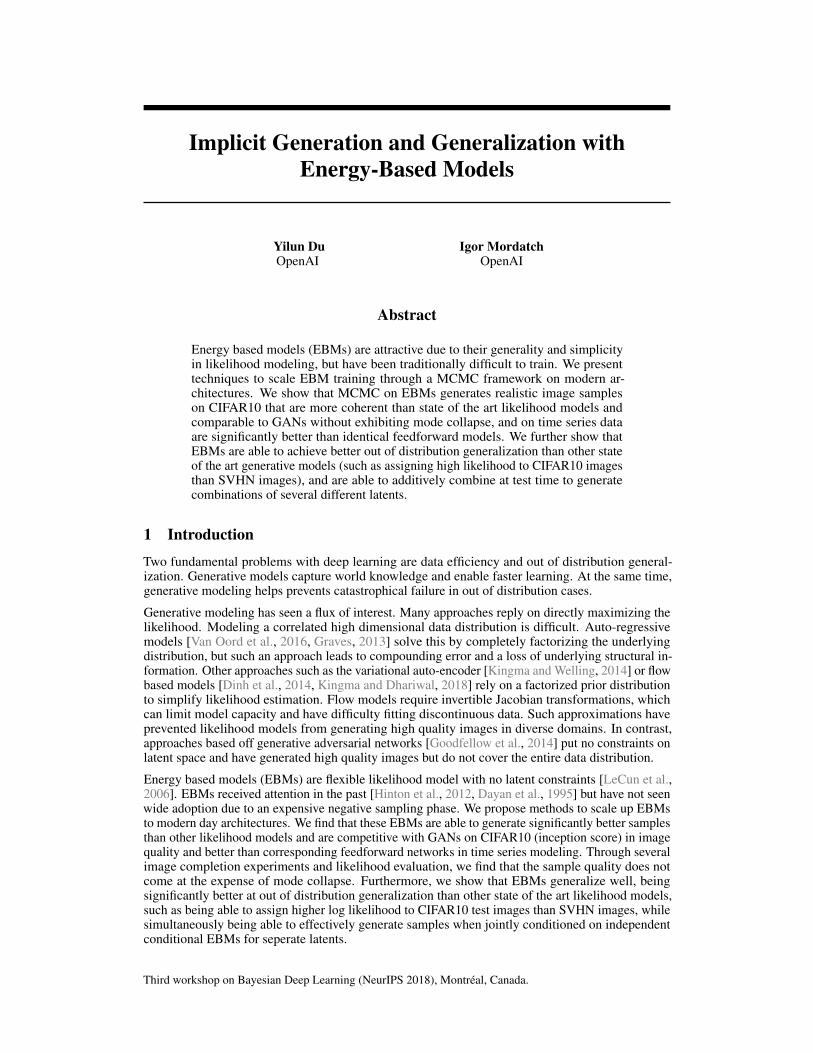
We provide unconditional generated images in Figure 2 and conditional generated images in Figure 3a.In Figure 2, we see that compared to Glow, are model is able to make much ore object like images.We show in Figure 12 that our generated images are not merely copies of images in the dataset.

We evaluate image quality of EBMs with Inception score [Salimans et al., 2016] and report comparisonwith other models Table 3b. As evidenced by qualitative examples, we find higher inception scoresthan PixelCNN (4.60) and is similar to performance to DCGAN (6.4) [Radford et al., 2016] inunconditional generation (6.43). One issue we found during evaluation is that LD sampling takeslarge amounts of time to explore all modes from random noise at test time, a problem mitigated by areplay buffer during training time. To mimic a replay buffers ability to increase sample diversity, weconsider alternate sampling from the last 10 snapshots of a model. Under this scheme, we are able toimprove scores to 6.79 and believe that additional improvements can be obtained by more explicitexploration, though we note that number are still lower than current state of the art unconditionalGAN models, likely due to reduced mode exploration.

5

Salt and Paper (0.1)

Inpainting

Ground Truth Initialization

Figure 4: Conditional EBM image restoration on images in the test set through MCMC. The rightcolumn shows failure (approx. 10% objects change with ground truth initialization and 30% ofobjects change in salt/pepper corruption or in-painting. Right column shows worst case of change.)

Figure 5: Illustration of cross class mapping using MCMC on a conditional EBM. The EBM isconditioned on a particular class but is initialized with an image from a separate class(left). Additionalimages in Figure 11

For conditional generation, we find that our inception score of 8.52 is higher than 8.09 in [Salimanset al., 2016] and is close to 8.59 in [Miyato et al., 2018]. Our conditional CIFAR10 scores arevery similar to state of the art GAN model scores. We believe a large reason for the increase incompetitiveness of conditional EBMs relative to unconditional EBMs is increased mode explorationduring evaluation / training time. With conditional EBMs, during test time evaluation, we able to ableto initialize generation of class images from images initially generated from other classes, allowingmore mode exploration.

4.2 Likelihood Evaluation

Quantitative Evaluation We found it difficult to estimate the partition function of EBMs tomeasure exact likelihood †. However, relative probability of data points can be evaluated by computingenergies of points. We found that our unconditional model had average energies of−0.00169±0.0196on the train dataset and 0.001454 ± 0.0176 on the test dataset. For conditional model, we foundenergies of 0.00198±0.0369 on the train dataset and 0.00751±0.0374 on the test dataset. The smallmean difference relative to individual standard deviation indicates EBMs assigns close likelihoods ontrain and test sets are not over-fitting to training images.

Image Restoration While unable to evaluate exact likelihood, we can measure the relative likeli-hood modeling of models through image decorruption on test images. If a model is a able to reliablyrestore and maintain test images, its likely that we have a good likelihood model of overall data. InFigure 4, we find that if we initialize sampling with images from the test set, images do not movesignificantly, indicating modes of probability at all test images. In Figure 4, we also test modelsability to inpaint and decorrupt images. We found in a large majority of cases, we are also able toreliably decorrupt images, indicating relatively little mode collapse. In comparison, GANs have beenshown to miss many modes of data and cannot reliably reconstruct many different test images [Yehet al.].

As an additional measure of likelihood modeling, we initialize conditional models with images fromimages from another class. We find in Figure 5 that energy models are still able to reliably convertthese images to images of the target class, showing additional signs of good likelihood models.

6

# Baseline FT Baseline + DA FT + DA

Accuracy 83.6 86.5 89.7 90.2Table 1: Test Accuracy on CIFAR10 with or without finetuning (FT) with or without data augmenta-tion (DA). We using horizontal flip and random crop data augmentations. Energy based fine-tuningallow better generalization.

Textures SVHN ConstantUniform

Uniform CIFAR10Mix

CIFAR10

Figure 6: Illustration of images from each of the out of distribution dataset.

4.3 Representation LearningWe further investigate representation learning in EBMs, which we measure by fine-tuning energymodels to a supervised classification task. We remove the last linear layer of our model and replace itwith a classification layer after pretraining in an unsupervised way. During training, we backpropogatethrough all weights and get results found in Table 1. We find EBMs learns representations that allowbetter generalization on CIFAR10. We believe even larger gains may be achieved by pre-training onlarger dataset or joint training.

4.4 Out of Distribution GeneralizationAn important evaluation metric for generative modeling is to measure how well models generalizeto out of distribution(OOD) images. If a generative model has learned a good probability datadistribution, the model should be able to assign lower probability to data from all other disjointdistributions. Curiously, however, as found in [Anonymous, 2019a], it appears current likelihoodmodels, such VAE, PixelCNN, and Glow models, are unable to distinguish data from disjointdistribution, and actual assigns higher likelihood to certain out of distribution images.

Similar to [Hendrycks and Gimpel, 2016], we propose a OOD metric where we take generativemodels trained on CIFAR10 and evaluate the AUROC score for classifying CIFAR10 test imagescompared to OOD images using log probability. We choose to evaluate on SVHN, Textures [Cimpoiet al., 2014], monochromatic uniform noise(all image pixels are the same value), uniform noiseand interpolations of separate CIFAR10 images. We choose the SVHN dataset for comparison toprevious works, Textures to test memorization of textures, monochromatic uniform noise to testfor memorization of smoothness, uniform noise as a sanity test for likelihood modeling, and imageCIFAR10 interpolation (where we mix two different CIFAR10 images) as a test of memorization oflow level image statistics. We provide illustration of out of distribution images in Figure 6.

As seen in Table 2, EBMs perform better out of distribution than other models. We provide histogramsof relative likelihoods for SVHN in Figure 7 which is also discussed in [Anonymous, 2019a]. Webelieve that reason for better generalization is two-fold. First, we believe that EBMs have flexiblestructure allowing global context when estimating probability without imposing constraints on†After training, we founding that using AIS [Neal, 2001] with HMC transitions took too long to explore

modes.

Model SVHN Textures Monochrome Uniform Uniform CIFAR10 Interpolation Average

PixelCNN ++ 0.32 0.33 0.0 1.0 0.71 0.47Glow 0.24 0.27 0.0 1.0 0.59 0.42EBM (ours) 0.63 0.48 0.30 1.0 0.70 0.62

Table 2: AUROC scores of out of distribution classification on different datasets

7

Figure 7: Histogram of relative likelihood for SVHN images vs CIFAR10 Test Images for Glow,PixelCNN++ and EBM models.

latents. In contrast, auto-regressive models model likelihood sequentially, making global coherencedifficult. In a different vein, flow based models must apply continuous transformations onto acontinuous connected probability distribution which makes it very difficult to model disconnectedmodes, consequently making it likely that large amounts of probability are wasted at connectionsbetween modes. Second, we believe that energy models have a negative sampling procedure toestimate the partition function, which allows the model to exhibit less bad local minima. However,we note that there is till much work that can be done to improve the out of distribution robustness ofgenerative models.

5 Time Series Prediction

2 4 6 8 10Prediction Steps

100

101

102

MSE

Err

or

Multistep Time Series Error

FeedForwardGradient MCMCMPPI MCMC

Figure 8: Multistep time series prediction MSEerrors (log scale). EBMs show out of distributiongeneralization by reduced long term rollout error.

To demonstrate the generality of our technique,we also explore the ability of energy functionsto model future predictions on time series. Weconsider two time series tasks; either predictingthe trajectory of a single moving ball.

5.1 Particle DynamicsTo test particle dynamics modeling, we simulateone moving ball with wall collisions, drag andfriction. We train models to predict the nextball positions given the past 3 positions using4500 training trajectories with 500 time-stepsand evaluate MSE of future state predictions on500 test trajectories. We compare training anenergy model with directly doing a feed-forwardprediction of state by modifying the last layer topredict the next state. We use the architecturegiven in Figure 14c and use either MPPI of LDto sample from. Details can be found in Sec-tion 8.6. The train feed-forward prediction onMSE error.

We present results of multistep time series pre-dictions at test time in Figure 8. When using model roll-outs, we find that energy functions havesignificantly lower error for multistep prediction despite higher initial error, compared to feed forwardnetworks. We believe this is due to EBMs being able to generalize better in out of distributionsituations that occur after a couple model rollouts. Interestingly, we find the MPPI based samplingmethods lead to better generalization than LD based sampling methods, probably partially due tobetter mode exploration during training time as the gradient may be biased to certain minima.

6 Combinatorial GeneralizationTo further evaluate generalization of EBMs, we consider sampling from the joint distribution ofseveral separately trained conditional EBMs on different latents. Due to the functional form ofEBMs, sampling from the joint distribution using LD is equivalent to taking gradient descent oneach respective conditional EBM with added noise. Sampling from the joint distribution testsgeneralization by leading to constraints/mode exploration likely not seen during training. We evaluate

8

Figure 9: Images generated by joint distribution of 4 conditional EBMs trained independently onscale, position, rotation and shape (left) with associated ground truth rendering (right). Despite neverbeing trained to sample with other conditional models, EBMS are able to generalize an aggregate ofthe latents

on the DSprites dataset [Higgins et al., 2017], which consists images of a single object varied byscale, position, rotation, and shape.

Latent Conditioning We found that it to we could effectively model conditional latent withconditional gains and biases following each convolution. Latents can be either continuous or discreteand are projected to the size of each gain or bias. We found latents of scale, position and rotationwere well. The latent of shape was difficult to learn, and we found that even our unconditionalmodels were not able to reliably generate different shapes which is also the case in [Higgins et al.,2017], perhaps due to the combinatorical explosion of different shapes at different scales. We furtherfound by incorporating latent sampling into proposal sampling during training, latents could also beeffectively inferred from images at test time.

Joint Conditioning In Figure 9, we provide generated images where we condition on 4 separateEBMs trained on conditioning of scale, position, rotation and shape on the entire DSprites dataset.We find that we are able to effectively sample from the joint distribution without significant loss insample quality (all factors except shape appeared to be preserved; the original conditional shapemodel is also unable to generate definitive shapes). We believe a unique advantage of EBMs isthe ability for sampling cost to scale linearly with the number separate conditional distribution asopposed to exponentially in the case of rejection sampling.

7 AcknowledgementsWe would like to thank Ilya Sutskever, Alec Radford, Prafulla Dhariwal, Dan Hendrycks, JohannesOtterbach and everyone at OpenAI for helpful discussions.

9

ReferencesAnonymous. Do deep generative models know what they don’t know? In Submitted to International Conference

on Learning Representations, 2019a. URL https://openreview.net/forum?id=H1xwNhCcYm. underreview. 7

Anonymous. The unreasonable effectiveness of (zero) initialization in deep residual learning. In Submitted toInternational Conference on Learning Representations, 2019b. URL https://openreview.net/forum?id=H1gsz30cKX. under review. 2, 13

Martin Arjovsky, Soumith Chintala, and Léon Bottou. Wasserstein gan. arXiv preprint arXiv:1701.07875, 2017.2, 4

M. Cimpoi, S. Maji, I. Kokkinos, S. Mohamed, , and A. Vedaldi. Describing textures in the wild. In Proceedingsof the IEEE Conf. on Computer Vision and Pattern Recognition (CVPR), 2014. 7

Peter Dayan, Geoffrey E Hinton, Radford M Neal, and Richard S Zemel. The helmholtz machine. NeuralComput., 7(5):889–904, 1995. 1

Laurent Dinh, David Krueger, and Yoshua Bengio. Nice: Non-linear independent components estimation. arXivpreprint arXiv:1410.8516, 2014. 1

Chelsea Finn, Paul Christiano, Pieter Abbeel, and Sergey Levine. A connection between generative adversarialnetworks, inverse reinforcement learning, and energy-based models. In NIPS Workshop, 2016. 2

Ian Goodfellow, Jean Pouget-Abadie, Mehdi Mirza, Bing Xu, David Warde-Farley, Sherjil Ozair, AaronCourville, and Yoshua Bengio. Generative adversarial nets. In NIPS, 2014. 1

Alex Graves. Generating sequences with recurrent neural networks. arXiv:1308.0850, 2013. 1

Kaiming He, Xiangyu Zhang, Shaoqing Ren, and Jian Sun. Deep residual learning for image recognition. InCVPR, 2015. 2

Dan Hendrycks and Kevin Gimpel. A baseline for detecting misclassified and out-of-distribution examples inneural networks. arXiv preprint arXiv:1610.02136, 2016. 7

Irina Higgins, Loic Matthey, Arka Pal, Christopher P Burgess, Xavier Glorot, Matthew Botvinick, ShakirMohamed, and Alexander Lerchner. Beta-vae: Learning basic visual concepts with a constrained variationalframework. In ICLR, 2017. 9

Geoffrey E Hinton. Training products of experts by minimizing contrastive divergence. Neural Comput., 14(8):1771–1800, 2002. 2

Geoffrey E Hinton, Nitish Srivastava, Alex Krizhevsky, Ilya Sutskever, and Ruslan R Salakhutdinov. Improvingneural networks by preventing co-adaptation of feature detectors. arXiv:1207.0580, 2012. 1, 2

Taesup Kim and Yoshua Bengio. Deep directed generative models with energy-based probability estimation.arXiv preprint arXiv:1606.03439, 2016. 2

Diederik P Kingma and Prafulla Dhariwal. Glow: Generative flow with invertible 1x1 convolutions. arXivpreprint arXiv:1807.03039, 2018. 1, 5

Diederik P. Kingma and Max Welling. Auto-encoding variational bayes. In ICLR, 2014. 1

Yann LeCun, Sumit Chopra, and Raia Hadsell. A tutorial on energy-based learning. 2006. 1, 2

Yang Liu, Prajit Ramachandran, Qiang Liu, and Jian Peng. Stein variational policy gradient. arXiv preprintarXiv:1704.02399, 2017. 3

Takeru Miyato, Toshiki Kataoka, Masanori Koyama, and Yuichi Yoshida. Spectral normalization for generativeadversarial networks. arXiv preprint arXiv:1802.05957, 2018. 3, 6, 13

Andriy Mnih and Geoffrey Hinton. Learning nonlinear constraints with contrastive backpropagation. Citeseer.2

Vinod Nair and Geoffrey E Hinton. Rectified linear units improve restricted boltzmann machines. In ICML,2010. 2

Radford M Neal. Annealed importance sampling. Stat. Comput., 11(2):125–139, 2001. 7

10

Alec Radford, Luke Metz, and Soumith Chintala. Unsupervised representation learning with deep convolutionalgenerative adversarial networks. In ICLR, 2016. 5

Tim Salimans, Ian Goodfellow, Wojciech Zaremba, Vicki Cheung, Alec Radford, and Xi Chen. Improvedtechniques for training gans. In NIPS, 2016. 5, 6

Tijmen Tieleman. Training restricted boltzmann machines using approximations to the likelihood gradient. InProceedings of the 25th international conference on Machine learning, pages 1064–1071. ACM, 2008. 3

Aaron Van Oord, Nal Kalchbrenner, and Koray Kavukcuoglu. Pixel recurrent neural networks. In ICML, 2016. 1

Max Welling and Yee W Teh. Bayesian learning via stochastic gradient langevin dynamics. In Proceedings ofthe 28th International Conference on Machine Learning (ICML-11), pages 681–688, 2011. 3

Grady Williams, Andrew Aldrich, and Evangelos A Theodorou. Model predictive path integral control: Fromtheory to parallel computation. Journal of Guidance, Control, and Dynamics, 40(2):344–357, 2017. 2, 3

Raymond A Yeh, Chen Chen, Teck-Yian Lim, Alexander G Schwing, Mark Hasegawa-Johnson, and Minh N Do.Semantic image inpainting with deep generative models. 6

Junbo Zhao, Michael Mathieu, and Yann LeCun. Energy-based generative adversarial network. arXiv preprintarXiv:1609.03126, 2016. 2

11

8 Appendix8.1 Derivation

Assuming that we have the following equation NLL objective with q(y) = p(y)

Ex∼pd(x)[E(x; θ) + log(Ey∼q(x)[e−E(y;θ)/q(y)])

]is equal to

Ex∼pd(x)[E(x; θ) + log(Ey∼q(x)[e−E(y;θ)/stop_gradient(e−E(y;θ))])

](11)

Taking the gradient of the above expression gets

Ex∼pd(x)[∇θE(x; θ)− Ey∼q(x)[∇θE(y; θ)]

](12)

Getting us an original objective of

Ex∼pd(x)[E(x; θ)− Ey∼q(x)[E(y; θ)]

]Alternatively, assuming q(y) = p(y) we can also directly derive the NLL gradient as

Ex∼pd(x) [∇θE(x; θ)]− ∇θZ(θ)Z(θ)

Focusing on the second term, assuming suitable regularity conditions, we bring the gradient insidethe integral to obtain

−∫(∇θE(x; θ)) ∗ eE(x;θ)dx

Z(θ)= Ex∼p(x)[∇θE(x; θ)]

Giving the other gradient of NLL of

Ex∼pd(x) [∇θE(x; θ)]− Ex∼p(x)[∇θE(x; θ)]

which is equivalent to Equation 12.

8.2 Algorithm Pseudocode

We present the pseudo-code for training EBMs with q(x) based off Langevin Dynamics in Algorithm 1.For training with MPPI, the MCMC step can be suitably changed.

8.3 Additional Qualitative Evaluation

We present images from a unconditional generation on ImageNet in Figure 10, which we generateusing the last 10 model snapshots of energy models. We find the presence of objects and scenes insome of the generated image with occasional hybrids (such as a presence of a toaster cat in middlebottom row).

We provide further images of cross class conversions using a conditional EBM model in Figure 11.Our model is able to convert images from different classes into reasonable looking images of thetarget class while sometimes preserving attributes of the original class.

Finally, we analyze nearest neighbors of images we generate in Figure 12.

8.4 Test Time Sampling Process

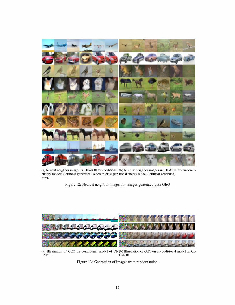
We provide illustration of image generation from conditional and unconditional EBM models startingfrom random noise in Figure 13 with small amounts of random noise added. Dependent on the imagegenerated there is slight drift from some start image to a final generated image. We typically observethat as sampling continues, much of the background is lost and a single central object remains.

We find that if small amounts of random noise are added, all sampling procedures generate a largeinitial set of diverse, reduced sample quality images before converging into a small set of high

12

Algorithm 1 Training Algorithm for EBMs with Langevin Dynamics(LD)

1: INPUT: number of proposal steps n, train dataset D, gradient clip threshold of V2: INITIALIZE: parameter θ of network and replay buffer B ← {}3: while Training do4: x+, l+ ← D5: x− ← B6: Replace 5% of the sample images in x− with U(0, 1)7: for i={1..n} do8: x− = x− - λ ∗ clip(∇θ(Eθ(x−, l+; θ)),−V, V ) +N(0, ε)9: end for

10: e_pos = E(x+, l+; θ), e_neg = E(stop_gradient(x−), l+; θ)11: Lossml = e_pos− softmax(stop_gradient(e_neg)) · e_neg12: Losskl = E(x−, l+; stop_gradient(θ)) . Only for time series data, otherwise set to 013: Lossreg = e_pos2 + e_neg214: Update E(x; θ) with∇θ(Lossml + Losskl + Lossreg)15: B ← x−

16: end while

probability/quality image modes that are modes of images in CIFAR10. However, we find that ifsufficient noise is added during sampling, we are able to slowly cycle between different images withlarger diversity between images (indicating successful distribution sampling) but with reduced samplequality.

Due to this tradeoff, we use a replay buffer to sample images at test time, with slightly high noisethen used during training time. For conditional energy models, to increase sample diversity, duringinitial image generation, we flip labels of images early on in sampling.

8.5 Model

We use the residual model in Figure 14a for conditional CIFAR10 images generation and the residualmodel in Figure 14b for unconditional CIFAR10 and Imagenet images. We found unconditionalmodels need additional capacity. Our conditional and unconditional architectures are similar toarchitectures in [Miyato et al., 2018].

We found definite gains with additional residual blocks. We further found that replacing globalsum pooling with a fully connected network also worked but did not lead to substantial benefits.We use the zero init in [Anonymous, 2019b] and spectral normalization on all weights. We useconditional bias and gains in each residual layer for a conditional model. We found it importantwhen down-sampling to do average pooling as opposed to strided convolutions. We use leaky ReLUsthroughout the architecture.

We use the architecture in Figure 14c for particle time series regression.

8.6 Training Hyperparameters

For CIFAR10 experiments, we use 60 steps of LD to generate negative samples. We use a replaybuffer of size of 10000 image. We scale images to be between 0 and 1. We clip gradients to havemagnitude of 0.01 and use a step size of 10 for each gradient step of LD. We use random noise withstandard deviation of 0.005. We train our model on 1 GPU for 2 days. We use the Adam Optimizerwith β1 = 0.0 and β2 = 0.999 with a training learning rate of 1e-4. We use a batch size duringtraining of 128 positive and negative samples. For both experiments, we clip all training gradientsthat are more than 3 standard deviations from the 2nd order Adam parameters. We use spectralnormalization on networks without backpropagating through the sampling procedure. We use theidentical setup for ImageNet 32x32 images, but train for 3 days on 1 GPU.

For trajectories, we use 20 steps of LD to generate negative samples. We use a noise standarddeviation 0.005. We use a batch size of 256 positive and negative samples. We found that a replaybuffer was not necessary. We use the Adam Optimizer with β1 = 0.0 and β2 = 0.999. For MPPI, weuse 30 steps of simulation with 5 noise simulations per step. We found spectral normalization to beoverly restrictive on trajectories so we instead backpropogate through the sampling procedure.

13

Figure 10: MCMC samples from unconditionalImageNet 32x32 EBM model

8.7 Tips And Failures

We provide a list of tips, observations and failures that we observe when trying to train energy basedmodels. We found evidence that suggest the following observations, though in no way are we certainthat these observations are correct.

We found the following tips useful for training.

• When training EBMs, we found the most important hyper-parameters to tune are MCMCtransition step sizes. We found that as long as this hyper-parameter was tuned correctlymodels would train stably.

• We found that it is important to use piecewise linear activations in EBMs (either ReLU orLeakyReLU). We found that other activations gave poor results and instability.

• When using residual networks, we found that performance can be improved by using 2Daverage pooling as opposed to transposed convolutions

• We found that group, layer, batch, pixel or other types of normalization appeared to signif-icantly hurt sampling, likely due to making MCMC steps dependent on surrounding datapoints.

• During a typical training run, we keep training until the sampler is unable to generateeffective samples (when energies of proposal samples are much larger than energies of datapoints from the training dataset). Therefore, to extend training for longer time periods, thenumber of sampling steps can be increased during long time periods for better generation.

14

Deer

Bird

Frog

Ship

Car

Airplane

Ship

Truck

Frog

Truck

Ship

Deer

Figure 11: Illustration of more cross class conversion applying MCMC on a conditional EBM. Wecondition on a particular class but is initialized with an image from a another class(left). We are ableto preserve certain aspects of the image while altering others.

• Generally, we would recommend first trying to train EBMs without a sampling loss withspectral normalization. Only if this doesn’t given satisfactory results would we recommendusing sampling loss, as this causes models to train slowly.

• We find that there appears to be a direct relationship between depth and sample quality.Simply increase model depth can easily increase generation quality.

• When adding noise when using MCMC sampling, we found that very low levels of noiseled to poor results. We found that high levels of noise allowed large amounts of modeexploration initially but quickly led to early collapse of sample (failure to explore modes).

We also tried the approaches below with the relative success levels indicated. For training of modelsin this paper, we do not use any of the additions listed below.

• We found that training ensembles of energy functions (sampling and evaluating on ensem-bles) to help a bit, but was not worth the added complexity.

• We found that multistep HMC or Adam based updates didn’t work well with sampling asthe momentum term appeared to add a large amount of noise to the sampling procedure. Wedid observe that include second order information helped training.

• We didn’t find much success with adding a gradient penalty term as it seemed to destablizesampling from the proposal distribution through LD.

• We found that a version of label discovery, where we assigned each data point a label withthe lowest energy (normalized by the average energy the label assigned to other point) toprovide some benefit. However, we found this gain in performance could also be obtainedby simply increase model parameters.

• We tried a version of proposal distillation where we tried to make each proposal step equalto the final outcome after a large number of proposal steps. We found small benefits but didnot found this computationally expensive.

• We tried training a separate network to help parametrize MCMC sampling but found thatthis made training very unstable. However, we did find that using some part of the originalmodel to parametrize MCMC (such as using the magnitude to energy to control step size) tohelp performance.

15

(a) Nearest neighbor images in CIFAR10 for conditionalenergy models (leftmost generated, seperate class perrow).

(b) Nearest neighbor images in CIFAR10 for uncondi-tional energy model (leftmost generated)

Figure 12: Nearest neighbor images for images generated with GEO

(a) Illustration of GEO on conditional model of CI-FAR10

(b) Illustration of GEO on unconditional model on CI-FAR10

Figure 13: Generation of images from random noise.

16

3x3 conv2d, 128

ResBlock down 128

ResBlock 128

ResBlock down 256

ResBlock 256

ResBlock down 256

ResBlock 256

Global Sum Pooling

dense→ 1

(a) Architecture used for condi-tional CIFAR10 experiments

3x3 conv2d, 128

ResBlock down 128

ResBlock 128

ResBlock 128

ResBlock down 256

ResBlock 256

ResBlock 256

ResBlock down 256

ResBlock 256

ResBlock 256

Global Sum Pooling

dense→ 1

(b) Architecture used for uncondi-tional CIFAR10 experiments

FC 32

Self Attention Block

Conv1D 128

Conv1D 128

dense→ 1

(c) Architecture used for Time Se-ries Experiments

17