Implications of a 2°C global temperature rise for

Canada’s natural resources

A report for WWF 30 November 2005

Acknowledgments

The authors would like to thank David Viner, Keith Brander, Steve Colombo, David Price, Lee Hannah, Gaétane Boisseau, Tony Iacobelli, Bob Rangeley and Michael Case for comments on earlier versions of the report.

Thanks to Dan Scott, David Welch, Camilo Mora and Ram Myers for their invaluable

help during especially during the scoping of the project. Thanks to Mark New, Mark Johnston, Paul Gray, Ron Neilson, Tony Hirsch, Rene

Laprise, Philippe Gachon, Stewart Cohen, Adam Markham, Jim Maslanik and Amanda Lynch for their interest and assistance at various stages of the project. ____________________________________________________________________________ Published in November 2005 by WWF-World Wide Fund For Nature (formerly World Wildlife Fund), Gland, Switzerland. Any reproduction in full or in part of this publication must mention the title and credit the above-mentioned publisher as the copyright owner. © text (2005) WWF. All rights reserved.

Implications of a 2°C global temperature rise for Canada’s natural resources

Edited by Tina Tin Executive Summary …………………………………………………………………………….. 4 Introduction ………………………………………………………………………………………6 Atlantic marine species Sea surface temperature changes in the Northwest Atlantic under a 2°C global temperature rise Gail L. Chmura, Sarah A. Vereault and Elizabeth A. Flanary …………………………………..9 Impacts of Sea Surface Temperature Changes on Marine Species in the Northwest Atlantic Lou Van Guelpen, Gerhard W. Pohle and Gail L. Chmura …………………………………….22 Ontario and boreal forests Projected tree distributions, tree migration rates, and forest types in Ontario under a 2°C global temperature rise Jay R. Malcolm, Danijela Puric-Mladenovic and Hua Shi……………………………………...52

Implications of climate change on disturbance regimes, carbon stocks, management and biodiversity of Canada’s boreal forests Jay R. Malcolm, Hua Shi and Danijela Puric-Mladenovic…………………………………….100

Implications of a 2°C global temperature rise for Canada’s natural resources

Executive Summary

Canada is a land of bounty. It is home to 10% of the world’s forests and freshwater resources; agriculture employs 15 million people and marine fisheries alone brings in an annual income of over CAN$2 billion. For a country where agriculture, forestry and fisheries make significant contributions to the national economy, Canada is especially susceptible to climate change.

In this study we examine the impacts of a 2°C increase in global temperature on aspects of the fishery and forestry sectors. Using the bioclimate (or climate) envelope approach, we established the climatic requirements of animal and plant species based on their current distributions. Mean global temperature is expected to rise by 2°C above pre-industrial levels during the period 2026-2060. Using output from global climate models for this period, we examine the climatic ranges of species under a 2°C warming to determine potential changes in species distribution. Our analysis is focused on marine species in the Northwest Atlantic and tree species in the province of Ontario; a review of literature extends our analyses to include freshwater phases of the Atlantic salmon as well as boreal forests nationwide.

Ectothermic animal species, such as fish and shellfish, are adapted to the temperature range of their natural environment. As climate changes, they are likely to redistribute according to preferred climatic conditions. We determined sea surface temperatures (SSTs) corresponding to the current ranges of three marine species in the Northwest Atlantic (excluding Hudson Bay) and then compared them to the predicted SSTs for the period 2044-2059. Under a 2°C increase in global temperature, SSTs in the Northwest Atlantic are expected to increase by 1.5-2.2°C. On the northeast U.S. continental shelf warming will be roughly equivalent in summer and winter, but in the waters of the Scotian and Newfoundland-Labrador shelves, greater warming in winter means that seasonality will be reduced.

We expect a 2°C warming to cause loss of favorable thermal habitat in the southern part of the range and no northward gain for both the Atlantic salmon (Salmo salar) and the Atlantic deep sea scallop (Placopecten magellanicus). The temperature regime shifts we foresee likely will seriously hinder attempts at the recovery of endangered Atlantic salmon populations, and the restoration of historic salmon runs where populations have been extirpated. The important freshwater recreational salmon fishery will see more frequent temporary closures of rivers to fishing due to warm water temperatures or because of fewer fish. A warming climate may benefit aquaculture, with expansion into waters of northern Nova Scotia, southern Newfoundland, and the Gulf of St. Lawrence. Scallop abundance is linked to the retention of their planktonic larvae in nearby waters, where SSTs play a major role in larval survival. A 2oC warming may eradicate the small scallop fisheries of in the vicinity of Cape Hatteras and maybe even in Virginia waters. With the increased SSTs predicted in northern waters the introduced Asian shore crab (Hemigrapsus sanguineus) is likely to invade shoreline habitats along the coast of Nova

4

Scotia, Gulf of St. Lawrence and parts of Newfoundland and Labrador, potentially covering the entire Canadian Atlantic. The crab’s high densities and large appetite for bivalves could seriously impact soft-shelled clam and blue mussel fisheries. Expanding populations of the Asian shore crab could also lead to considerable changes in native shoreline communities.

During the period 2040-2050, the province of Ontario is expected to warm by 1.4-3.4°C. Using information on tree populations in Ontario and the eastern United States, we applied climate, soil, topographic, and land-use information to model existing and future tree distributions in Ontario. Our results indicated the potential for dramatic change in Ontario's forests under a 2°C warming. The modeled climate envelopes (suitable habitats) of most species shifted significantly northward. Declines in dominance were projected in many regions for key commercial species such as black spruce, jack pine, and sugar maple. Changes in forest types were widespread as more southerly species (including species not currently found in the province) moved northwards. However, a number of factors, including fragmentation of habitat and limitations in dispersal capabilities, suggest that tree species will be unable to migrate fast enough to keep up with the enormously high migration rates that our models projected. The implication is that future ecosystem composition increasingly will be driven by the climatic tolerances of species, with only the more climatically tolerant species persisting at a site. Increased stress brought about by climatic conditions outside of usual climate envelopes will presumably make species more susceptible to disease and pest problems. Species may become relegated to refugia where conditions are still satisfactory.

The production of maple syrup may be significantly reduced if temperatures remain above freezing during the sugaring-off period. Although small from a GDP perspective, effects on local economies and regional heritage could be large.

Climate change is also expected to increase the frequency and severity of disturbances, including fires and insect outbreaks in Canada’s boreal forests. Increases in disturbances could result in younger forests which would reduce the amount of harvestable timber. This could also lead to loss of habitat for boreal species that are already under pressure from habitat fragmentation and logging activities. Warmer temperatures and forest fires are expected to reduce carbon stocks in boreal forests. In the search for appropriate adaptive responses to climate change, the different management goals of sustainability, biodiversity, and timber harvest should not be mutually exclusive.

5

Introduction

This report is the third in a series of studies focusing on the worldwide impacts of a 2°C rise in global temperature. Earlier studies have examined changes in Arctic vegetation, sea ice cover, impacts on livelihoods of indigenous people, extreme weather events in the Mediterranean and impacts on Mediterranean tourism and agriculture (Rosenstrater, 2005; Giannakopoulos et al., 2005). In this study, we use the climate (or bioclimate) envelope approach to examine the implications of a 2°C warming on two aspects of Canada’s natural resources – Atlantic marine species and Ontario and boreal forests.

On a macro-scale, climate has been shown to be the dominant influence on species distribution (Pearson and Dawson, 2003). The “climate envelope” of a species can be described by the climatic conditions encompassing the current distribution of a species. Under climate change scenarios, this climate envelope is likely to shift in location, indicating the potential future distribution of the species (Gitay et al., 2001). This relatively simple approach has been shown to provide a useful first approximation as to the potentially dramatic impact of climate change on biodiversity (Pearson and Dawson, 2003), and a number of studies have successfully used this approach to highlight the extinction risks of plant and animal species under climate change (e.g., Thomas et al., 2004; Thuiller et al., 2005). However, critics point out that the current range of a species does not necessarily represent its full potential range (Araújo et al., 2005) and climate envelope models do not account for important factors, such as predation, competition, dispersal limitation, speed of anticipated climate change and habitat fragmentation (Hampe, 2004). Hence, predictions from these models could lead to artificially optimistic scenarios of climate change impacts (Hampe, 2004).

In our study, climate envelopes are described by sea surface temperatures (for marine species) or by a statistical correlation between species abundance, and climate, soil, topographic, and land-use conditions (for tree species) in the current range of the species. For tree species, dispersal limitation and fragmentation play an important role in species distribution and these topics are discussed in Chapters 3 and 4. Dispersal limitation is less of a problem for marine species, as many are dispersed by a floating larval stage. However, changes in predators or prey can have a cascading effect on levels of the food chain in marine communities. For instance, the invasive Asian shore crab, discussed in Chapter 2, is expected to expand along the shores of the Canadian Atlantic and restructure communities of coastal organisms.

Our study is a first investigation into the effects of an increase a 2°C rise in global temperature on some of Canada’s natural resources. Although they cannot account for all of the complex dynamics of the natural ecosystems being modeled, they provide a first-order, conservative estimate of the potential magnitude and pattern of future change.

In order to make use of the climate envelope approach, it is necessary to obtain climate conditions corresponding to a 2°C rise in global temperature. New (2005) examined monthly data from six coupled ocean-atmosphere global climate models, each driven by several forcing scenarios. For each model, control-run surface temperature data were used to calculate a “pre-industrial” mean temperature climatology, and these were spatially averaged to calculate a global mean pre-industrial surface temperature. For each climate change simulation, the global temperature fields were spatially averaged to calculate time-series of global mean annual temperature, which were then differenced from the “pre-industrial” global mean temperature. The resulting global mean temperature-anomaly series were then smoothed with a 21-year moving average, and the date at which the 21-year mean global temperature anomaly exceeded

6

2°C was taken as the time of 2°C global temperature change. The time at which the simulated global mean temperature exceeds the control run global mean by 2°C ranges from between 2026 and 2060 (Figure 1).

Figure 1. The color of each line indicates the emission scenarios used. A2 and B2 are scenarios from the IPCC SRES families. IS92agg and IS92ags represent the IPCC IS92a scenario with greenhouse gas only. IS92ags represents the IS92a scenario with greenhouse gas and aerosols. The models used are: CCSRNIES from the Centre for Climate System Research National Institute for Environmental Studies; CGCM1/2; CSIROMk2 from Australia’s Commonwealth Scientific & Industrial Research Organization; ECHAM4; GFDLR30 from Geophysical Fluid Dynamics Laboratory; HADCM3 from the U.K. Meteorological Office. (New, 2005)

Following the results from New (2005), the present study derives climatic conditions under a 2°C rise in global temperature from five global climate models and two emission scenarios for the periods 2044-2059 (for marine species) and 2040-2050 (for tree species) in the present study (Table 1). These climatic conditions are then applied to the climate envelope models in order to examine the potential changes in the distribution of species under a 2°C warming.

7

Table 1. The study periods, emission scenarios and global climate models used in the present study. Canadian Atlantic marine species

(Chapters 1 and 2) Tree species in Ontario (Chapter 3)

Study period 2044-2059 2040-2050 Emission scenarios SRES A2, B2 SRES A2, B2

CGCM2 (Canadian Centre for Climate Modeling and Analysis)

CGCM2

CSIRO Mk2 (Australia’s Commonwealth Scientific & Industrial Research Organization)

CSIRO Mk2

CCSR/NIES AGCM CCSR OGCM (Centre for Climate System Research National Institute for Environmental Studies)

HadCM3 (U.K. Meteorological Office)

Models

GFDL R30 C (Geophysical Fluid Dynamics Laboratory)

References Araújo, M.B, Pearson, R.G., Thuiller, W. and Erhard, M. 2005. Validation of species-climate

impact models under climate change. Global Change Biology 11: 1504-1513. Giannakopoulos, C., Bindi, M., Moriondo, M., LeSager, P. and Tin, T. 2005. Climate change

impacts in the Mediterranean resulting from a 2°C global temperature rise. WWF, Gland, Switzerland. 75pp.

Gitay, H., Brown, S., Easterling,W. & Jallow, B., eds. 2001. Ecosystems and their goods and services. In McCarthy, J.J., Osvaldo, F.C., Leary, N.A., Dokken, D.J. & White, K.S., eds. 2001. Climate change 2001: impacts, adaptation and vulnerability. Contribution of Working Group II to the Third Assessment Report of the Intergovernmental Panel on Climate Change, pp. 235-342. Cambridge, UK, Cambridge University Press. 1042 pp.

Hampe, A. 2004. Bioclimate envelope models: what they detect and what they hide. Global Ecology and Biogeography. 13: 469-476.

New M., 2005. Arctic climate change with a 2°C global warming. In Rosentrater L. (Ed.): Evidence and Implications of Dangerous Climate Change in the Arctic, WWF International Arctic Programme..

Pearson, R.G., and T.P. Dawson. 2003. Predicting the impacts of climate change on the distribution of species: are bioclimate envelope models useful? Global Ecology and Biogeography 12: 361–371.

Rosenstrater, L. (ed.) 2005. Evidence and Implications of Dangerous Climate Change in the Arctic, WWF International Arctic Programme. 75pp. Thomas C.D. and 18 others. 2004. Extinction risks from climate change. Nature, 427, 145–148. Thuiller W., Lavorel S., Araújo M.B., Sykes M.T. and Prentice I.C. 2005. Climate change threats

to plant diversity in Europe. PNAS 102 (23), 8245–8250.

8

Chapter 1 Sea surface temperature changes in the Northwest Atlantic under a 2°C global temperature rise Gail L. Chmura, Sarah A. Vereault and Elizabeth A. Flanary Department of Geography (and Global Environment and Climate Change Centre) McGill University Montreal, Quebec Abstract

To enable assessment of the impact of greenhouse warming on marine species, we examined future changes in sea surface temperatures (SSTs) for the Northwest Atlantic (excluding Hudson Bay) by statistically downscaling output from four global climate models and two emission scenarios. Our analyses focused on the months of February and August, which generally represent extremes in winter and summer SSTs in this region. We considered changes in SSTs in the context of three Large Marine Ecosystems, areas internationally designated for fisheries management: the Northeast U.S. Continental Shelf, the Scotian Shelf and the Newfoundland-Labrador Shelf. This region encompasses the frontier between waters within the jurisdiction of the United States and Canada, as well as important international fishing grounds, and thus has important economic significance for the U.S. and Canada as well as other countries.

For the period 2044-2059, at which time average global air temperature is expected to have risen by 2°C, SSTs in the Northwest Atlantic is expected to increase by 1.5-2.2°C. In the Northeast U.S. Continental Shelf there will be roughly equivalent increases in summer and winter SSTs, but greater warming in winter means that seasonality will be reduced in waters of the Scotia and Newfoundland-Labrador Shelves. All models show winter warming on the northeast coast of Labrador, Canada, the Gulf of St. Lawrence and the region immediately north of Cape Hatteras, North Carolina in the U.S. Differences among our model projections were greater than differences between scenarios, but there was consistency within the ensemble. A limitation of our study is that ocean circulation is not adequately represented in global climate models.

9

Introduction Greenhouse warming is expected to cause increased temperatures in the sea as

well as on land. Global climate models (Atmosphere-Ocean General Circulation Models = AOGCMs) predict that sea surface temperatures in the North Atlantic will increase by 2°C by 2059. This increase is expected to be accompanied by significant impacts on the distribution and abundance of marine organisms, particularly in the Northwest Atlantic where temperature gradients are sharp and biogeographic ranges of species compressed, as compared to other regions, such as the Northeast Atlantic (e.g., Dale 1996).

Assessing the impact of greenhouse warming on marine species is complicated by two factors. The projections of AOGCMs vary regionally (Cubasch et al. 2001) and the spatial resolution model output is at too coarse a scale to be practical for impact studies. In this study we address these two complications by downscaling output from AOGCMs and comparing multiple models and emissions scenarios to determine where projections are regionally consistent.

To assess the consistency among models we compare the change in sea surface temperatures projected by four AOGCMs through two emission scenarios in the context of three large marine ecosystems (LMEs) of the Northwest Atlantic. The size of LMEs, >200,000 km2 (Alexander 1993), is appropriate for application of the coarse spatial resolution of AOGCM output.

Large Marine Ecosystems are characterized by special hydrographic conditions that contribute to extensive fish populations that form the basis of commercial fisheries. Sustainability of these fish populations are a prime objective of LME management. Understanding of potential changes in sea surface temperatures thus, is critical to management of LMEs as increased water temperatures may cause shifts in populations of harvestable fish and their prey.

This region encompasses the frontier between waters within the jurisdiction of the United States and Canada, as well as important international fishing grounds (Figure 1). Thus, changes in marine resources here have significant economic impacts for the U.S. and Canada as well as other countries. Data and methods Modern Sea Surface Temperatures

For modern sea surface temperatures we used the NSIPP climatology data set which represents Advanced Very High Resolution Radiometer (AVHRR) sea surface temperatures for the years 1985-1997 as monthly averages calculated from pentad averages (Casey & Cornillon, 1999). To reduce computational costs we limit our analyses to the months of February and August, which generally represent extremes in winter and summer SSTs our target region, which excluded Hudson Bay. Our February data includes sea ice which produces anomalous SSTs, so we excluded these areas from our analyses.

10

11

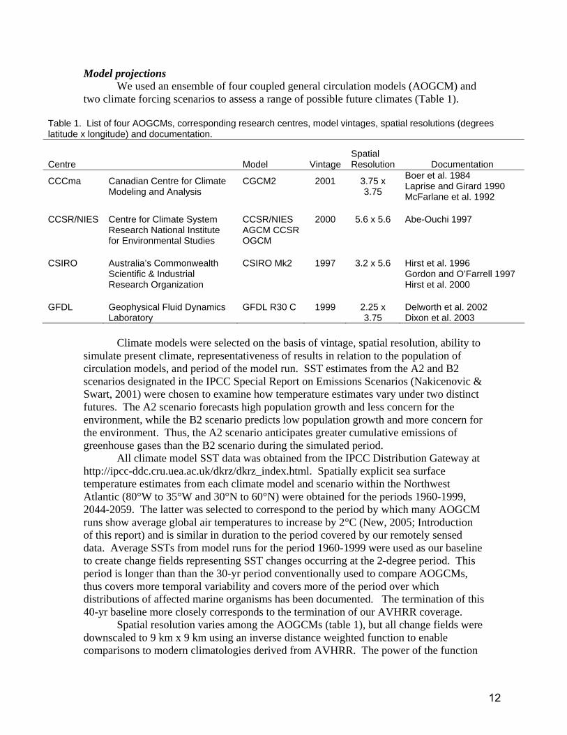
Model projections We used an ensemble of four coupled general circulation models (AOGCM) and

two climate forcing scenarios to assess a range of possible future climates (Table 1).

Table 1. List of four AOGCMs, corresponding research centres, model vintages, spatial resolutions (degrees latitude x longitude) and documentation.

Centre Model VintageSpatial Resolution Documentation

CCCma Canadian Centre for Climate Modeling and Analysis

CGCM2 2001 3.75 x 3.75

Boer et al. 1984 Laprise and Girard 1990 McFarlane et al. 1992

CCSR/NIES Centre for Climate System

Research National Institute for Environmental Studies

CCSR/NIES AGCM CCSR OGCM

2000 5.6 x 5.6 Abe-Ouchi 1997

CSIRO Australia’s Commonwealth

Scientific & Industrial Research Organization

CSIRO Mk2 1997 3.2 x 5.6 Hirst et al. 1996 Gordon and O’Farrell 1997 Hirst et al. 2000

GFDL Geophysical Fluid Dynamics

Laboratory GFDL R30 C 1999 2.25 x

3.75 Delworth et al. 2002 Dixon et al. 2003

Climate models were selected on the basis of vintage, spatial resolution, ability to

simulate present climate, representativeness of results in relation to the population of circulation models, and period of the model run. SST estimates from the A2 and B2 scenarios designated in the IPCC Special Report on Emissions Scenarios (Nakicenovic & Swart, 2001) were chosen to examine how temperature estimates vary under two distinct futures. The A2 scenario forecasts high population growth and less concern for the environment, while the B2 scenario predicts low population growth and more concern for the environment. Thus, the A2 scenario anticipates greater cumulative emissions of greenhouse gases than the B2 scenario during the simulated period.

All climate model SST data was obtained from the IPCC Distribution Gateway at http://ipcc-ddc.cru.uea.ac.uk/dkrz/dkrz_index.html. Spatially explicit sea surface temperature estimates from each climate model and scenario within the Northwest Atlantic (80°W to 35°W and 30°N to 60°N) were obtained for the periods 1960-1999, 2044-2059. The latter was selected to correspond to the period by which many AOGCM runs show average global air temperatures to increase by 2°C (New, 2005; Introduction of this report) and is similar in duration to the period covered by our remotely sensed data. Average SSTs from model runs for the period 1960-1999 were used as our baseline to create change fields representing SST changes occurring at the 2-degree period. This period is longer than than the 30-yr period conventionally used to compare AOGCMs, thus covers more temporal variability and covers more of the period over which distributions of affected marine organisms has been documented. The termination of this 40-yr baseline more closely corresponds to the termination of our AVHRR coverage.

Spatial resolution varies among the AOGCMs (table 1), but all change fields were downscaled to 9 km x 9 km using an inverse distance weighted function to enable comparisons to modern climatologies derived from AVHRR. The power of the function

12

was set to two. A minimum of eight neighboring data points were used for each interpolation. Interpolation through land was eliminated by using a barrier mask. The barrier limited the search for neighboring data to only those input sample points on the same side of the barrier as the processed cell. Interpolation was performed by the Spatial Analyst extension in ArcMAP (ESRI, V 8). Results

The zonal means of the interpolated SST change fields for each LME, scenario are depicted in Figure 2. Regional variation in SSTs is shown in Figure 3.

Comparison of Models and Scenarios

Differences among model projections are not consistent, i.e., no model consistently projects the lowest changes or highest changes (Figure 2), but there is consistency within the ensemble. Degree of agreement in projections within the ensemble can be assessed by examining the ratio of the ensemble mean to the standard deviation of the ensemble projections. An ensemble mean exceeding the standard deviation is taken as a constant response among models (Cubasch et al. 2001). Although this ratio is greater than one for all scenarios and months the consistency of agreement varies with month (Figure 4). Variability among projections is greater in February. Absolute differences among the mean projections are greater in February than August so this is not simply an artifact of the lower means in February. In all cases model projections were the most consistent for the Northeast U.S. Continental Shelf.

Interestingly, differences in projections within the model ensemble are greater than differences between scenarios A2 and B2 for a single model. Differences among model projections were much greater than differences between the two scenarios (Figure 3). Modern Conditions

Average modern SSTs calculated from AVHRR data averaged over the years 1985-1997 in August and February for each LME are shown in table 2. As expected, the Scotian Shelf has August and February temperatures intermediate to the Northeast U.S. Continental Shelf and the Newfoundland-Labrador Shelf. However, the Scotian Shelf is characterized by the highest seasonal variability, i.e., a 17.4°C difference in SSTs from summer to winter. The seasonal variation on the Scotia Shelf is 18% greater than that of the Northeast U.S. Continental Shelf and 45% greater than what occurs on the Newfoundland-Labrador Shelf.

Table 2. Sea surface temperatures derived from AVHRR averaged across large marine ecosystems Large Marine Ecosystem

Northeastern U.S. Continental

Shelf Scotian Shelf

Newfoundland – Labrador Shelf

February 5.44 -0.07 -0.57 August 20.13 17.29 11.39

13

U.S. Northeast Continental Shelf

Cha

nge

in S

ST ºC

-2

0

2

4

6

8

10

-2

0

2

4

6

8

10

Scotian Shelf

Cha

nge

in S

ST ºC

-2

0

2

4

6

8

10

-2

0

2

4

6

8

10

Newfoundland-Labrador Shelf

CCCmaCCSR

CSIRO

GFDL

Ensemble

CCCmaCCSR

CSIRO

GFDL

Ensemble

Cha

nge

in S

ST ºC

-2

0

2

4

6

8

10

-2

0

2

4

6

8

10

A2 scenarioB2 scenario

February August

Figure 2. Zonal average and standard deviation of SST change projected by four AOGCM in each LME for the A2 and B2 scenarios. Ensemble refers to the average of the four models.

14

15

Figure 4. Ratio of mean to standard deviation for ensemble mean change fields zonally averaged over each LME.

Average differences in modern SSTs between the Northeast U.S. Continental

Shelf and the Scotian Shelf are greater in the winter when Scotian Shelf waters are 5.5°C colder. In contrast, the greater difference in SSTs between the Scotia Shelf and more northern waters of the Newfoundland-Labrador Shelf occurs during summer, as reflected by an average difference of 5.9°C in August. Changes in LMEs

The zonal means of our interpolated model projections indicated increased SSTs in each period and scenario for all LMEs, but with spatial variability (Figures 3). August SSTs increased throughout the study region, but projections of February SSTs were not consistently higher. The extent of change also varied among the LMEs.

Increased SSTs were projected throughout the Northeast U.S. Continental Shelf waters for both seasons (Figures 2). The ensemble zonal average increases in February and August were similar: 1.5°C in both scenarios in February and 1.6 (A2) to 1.7°C (B2) in August.

Decreased SSTs were indicated in some locations of the Scotian and Newfoundland-Labrador Shelves (Figure 3). Our interpolated change field for CCMA showed decreases in both scenarios and both months for parts of the Newfoundland-Labrador Shelf, but only in February for the Scotian Shelf.

Zonal ensemble mean changes were higher on the Scotian Shelf than the Northeast U.S. Continental Shelf (Figure 2). As with the Northeast U.S. Continental Shelf, the results for both scenarios were similar on the Scotian Shelf. The zonal average

16

temperature of the Scotian Shelf could increase by 2.2°C through both scenarios in February, but only by 1.5°C (A2) to 1.6°C (B2) in August.

The zonal ensemble mean SSTs calculated for the Newfoundland-Labrador Shelf show a pattern of increase similar to that of the Scotian Shelf, but the magnitude of change fell between that and the Northeast U.S. Continental Shelf. The ensemble mean February temperature increased by 2.1°C in both scenarios in February and 1.1°C (A2) to 1.3°C (B2) in August (Figure 2).

Critical areas of warming

At a finer scale, we can identify at least three areas within LMEs where warming is notable. Although the magnitude of change varies, all models show winter warming on the northeast coast of Labrador, Canada, the Gulf of St. Lawrence and the region immediately north of Cape Hatteras, North Carolina in the U.S. Discussion Models and Scenarios

Variability in zonal mean SSTs of the NW Atlantic generally is greater among the four models than between the A2 and B2 scenarios. Spatial variability among AOGCMs is widely recognized (Giorgi et al. 2001), but comparison of different scenarios may have revealed a greater difference. For instance, an application of the HadCM3 (not used in this study) to examine projected mean annual SSTs in the North Sea showed that the B1 scenario produced lower SSTs than the A2 or B2 (Clark et al. 2003).

Spatial variability in model output is due to a number of factors. One factor is that models vary in horizontal (table 1) or vertical resolution of the atmosphere (McAvaney 2001). Models also differ in the manner in which they simulate clouds and humidity, two parameters with important climate feedbacks. Of particular importance to the northern North Atlantic is the varying treatment of sea ice, as well as the leads and polynyas within it (McAvaney 2001).

Complications in treatment of sea ice may, in part, explain why ensemble variability is lowest in the Northeast U.S. Continental Shelf - which has no sea ice. It may also contribute to the higher ensemble variability in winter for the Scotian and Newfoundland-Labrador Shelves.

The A2 scenario is characterized by higher fossil fuel emissions, thus greater greenhouse gas forcing, yet SSTs were similar or higher than those calculated for the B2 scenarios. This pattern parallels that reported for global average surface air temperatures (Cubasch et al. 2001). Warming is reduced in the A2 scenario because it is also characterized by higher emission of sulfur dioxide, which has a negative radiative forcing. These aerosols stimulate cloud formation providing a cooling effect that reduces the impact of greenhouse gases (Mitchell and Johns 1997). (In model projections for future years the level of emission of greenhouse gases in the A2 scenario eventually become the dominant determinant of climate change, overwhelming the cooling effects of sulfur dioxide emissions.)

Within the output of any single model there is no systematic shift in maximum or minimum SSTs among the three LMEs examined here – nor was one expected. Levitus et al. (2005) summarize the two major reasons why greenhouse warming does not cause

17

uniform heating of the ocean. First, regional warming rates are affected by natural and anthropogenic aerosols, as well as black carbon which are not well mixed geographically. Second, changes in the global radiation balance may induce changes in atmosphere and ocean circulation, thus affect the net flux of heat across the air-sea interface on a regional basis.

There are major differences in the timing of SST increases. In the waters of the Northeast U.S. Continental Shelf there will be roughly equivalent increases in summer and winter SSTs, but greater warming in winter means that seasonality will be reduced in waters of the Scotia and Newfoundland-Labrador Shelves. Uncertainties

The greatest limitation of our study is its dependence on AOGCM output which does not reflect important characteristics of ocean circulation or their response to cyclical climate perturbations, such as the North Atlantic Oscillation. The coarse spatial resolution of AOGCMs is a major limitation in deriving more realistic spatial patterns of SSTs. Spatial variability in sea surface temperatures of the Northwest Atlantic is largely driven by circulation of ocean currents (Townsend et al. 2004). Two major currents are the Labrador Current that transports cold waters southward as far as the coast of New York and the Gulf Stream which transports warm waters northeastward towards Europe. These large currents and other smaller features of ocean circulation are too small to be realized in the output from AOGCMs thus our downscaling reflects coarse inshore-offshore temperature trends, but not other smaller scale variations that may result in SSTs warmer or colder than predicted.

The NAO dictates climate variability from the eastern seaboard of the United States to Siberia and from the Arctic to the subtropical Atlantic (Hurrell and Dickson 2004). It is a north-south oscillation in atmospheric pressure centered over Iceland and the subtropical Atlantic from the Azores across the Iberian Peninsula that drives annual to decadal scale temperature changes over land and sea. The NAO affects mostly winter SSTs – in a seesaw fashion. The “positive” mode of its oscillation is associated with lower sea surface temperatures over the subpolar NW Atlantic, but higher temperatures in southern waters (Visbeck et al. 2004). The NAO affects circulation of important currents on the NW Atlantic, such as the Labrador Current. For instance, a weak NAO may allow intensified southward transport of the cold Labrador Current and displacement of the Gulf Stream further south (Loder et al. 2001). The relationship of the NAO to circulation changes and long-term climate change are complex and still being sorted out by scientists.

Annual and decadal fluctuations of sea surface and deeper water temperatures are spatially variable and difficult to predict. Reconstructions of ocean temperature records reveal that variability of 2°C and higher (Keigwin et al. 2003; Loder et al. 2004).

Short term ocean fluctuations in ocean temperatures could have variable effects on the expression of global warming. Variability in ocean temperatures is greater than SST changes predicted with a 2°C global warming (Figure 2). Thus, short-term decreases in SSTs could temporarily counter the impacts of greenshouse warming, particularly in short-lived species. However, short-term increases would exacerbate conditions caused by greenhouse warming – accelerating impacts on sensitive species.

18

Our predictions are restricted to sea surface temperatures, a problem in their application to species such as scallops that, as adults may live in waters as deep as 200 m. Bottom waters are slower to respond to climate changes and temperature changes in deeper waters may not be directly proportional to changes SSTs. Studies of waters over the continental shelf from Nova Scotia to Georges Bank reveal that in winter bottom water temperatures may be 2 to 8ºCcolder than sea surface temperatures (Loder et al. 2001). During a period of warmer waters in the 1970s northern NW Atlantic SSTs were as much as 8ºC higher than bottom water temperatures. This variation decreased towards the southern end of Georges Bank where differences in from surface were ~2ºC. During the colder 19602 there was less differences between SSTs and bottom water temperatures were reduced.

Summary and Conclusions Sea surface temperatures of the Northwest Atlantic will increase, but there is a

substantial difference in the pattern between the Northeast U.S. Continental Shelf and the Scotian and Newfoundland-Labrador Shelves, the latter primarily Canadian waters. The seasonality that distinguishes the two northern LMEs will be considerably reduced, with possible effects on the dominance of pelagic or benthic food webs. SSTs of the Northeast U.S. Continental Shelf will increase throughout the year, but there will be a greater increase in winter SSTs in the Canadian LMEs. Thus winter lows will be less of a barrier for migration of species and allow shifts of those intolerant of the higher SSTs projected for the Northeast U.S. Continental Shelf. Cape Hatteras, North Carolina is the southern point of the biogeographic range of a number of marine organisms and warming there may cause retraction of their southern range. This, accompanied by warming to the north is likely to drive a northward shift of biogeographic ranges of some marine organisms. However, higher winter SSTs will further contribute to reduction of Arctic sea ice, which is a critical element of the habitat of many species there.

In our examination of three NW Atlantic LMEs we find no single model or scenario consistently produces maximums or minimums in SST change. Thus, future studies examining variability in this region should consider ensembles of different models as well as scenarios.

Acknowledgements This research was funded by the Canadian Climate Change Impacts and Adaptation Program, project A515 and the Natural Sciences and Engineering Research Council of Canada. We thank Hong Jiang for programming assistance and colleagues J. Seaquist and R. Sieber for advice on GIS analyses.

19

References Abe-Ouchi A (1997) Outline of coupled atmosphere ocean GCM and global warming

experiments (in Japanese). Internal report 2, 117-130, Centre for Climate System Research (CCSR), University of Tokyo, Japan.

Alexander LM (1993) Large marine ecosystems, a new focus for marine resources management. Marine Policy 186-198.

Boer GJ, McFarlane NA, Laprise R, Henderson JD and Blanchet J-P (1984) The Canadian Climate Centre Spectral atmospheric general circulation model. Atmosphere-Ocean, 22, 397-429.

Casey KS, Cornillon P (1999) A comparison of satellite and in situ-based sea surface temperature climatologies. Journal of Climate, 12, 1848-1862.

Cubasch U, Meehl GA, Boer GJ, Stouffer M, Dix M, Noda A, Senior CA, Raper S, Yap KS (2001) Projections of future climate change. Pp. 525-582 In Houghton JT, Ding Y, Griggs DJ, Noguer M, VAN DER Linden PJ, Dai X, Maskell K, Johnson CA (eds.) Climate change 2001: the scientific basis, contribution of working group 1 to the third assessment report of the intergovernmental panel on climate change. Cambridge University Press.

Dale, B (1996) Chapter 31 Dinoflagellate cyst ecology: modeling and geological applications; Pp 1249-1279 IN Jansonius J McGregor DC (eds) Palynology, principles and applications. American Association of Stratigraphic Palynologists Foundation, vol 3.

Delworth TL, Stouffer RJ, Dixon Kw, Spelman Mj, Knutson TR, Broccoli AJ, Kushner PJ, Wetherald RT (2002) Review of simulations of climate variability and change with the GFDL R30 coupled climate model. Climate Dynamics, 19,555-574.

Dixon KW, Delworth TR, Knutson TR, Spelman MJ, Stouffer RJ (2003) A comparison of the climate change simulations produced by two GFDL coupled climate models. Global and Planetary Change, 37, 81-102.

ESRI (2005) ArcGIS version 9.0. Environmental Systems Research Institute, Redlands, CA.

Giorgi F, Hewitson B, Christensen J, Hulme M, Von Storch H, Whetton P, Jones R, Mearns L. Fu C (2001) Regional climate information – evaluation and projections. Pp. 583-638 IN Houghton JT, Ding Y, Griggs DJ, Noguer M, VAN DER Linden PJ, Dai X, Maskell K, Johnson CA (eds.) Climate change 2001: the scientific basis, contribution of working group 1 to the third assessment report of the intergovernmental panel on climate change. Cambridge University Press.

Gordon HB, O’Farrell SP (1997) Transient climate change in the CSIRO coupled model with dynamic sea ice. Monthly Weather Review, 125, 875-907.

Gordon C, Cooper C, Senior et al. (2000) The simulation of SST, sea ice extents and ocean heat transports in a version of the Hadley Centre coupled model without flux adjustments. Climate Dynamics, 16,147-168.

Hirst AC, Gordon HB, O’Farrell SP (1996) Global warming in a coupled climate model including oceanic eddy-induced advection. Geophysical Research Letters, 23, 3361-3364.

Hirst AC, O'Farrell SP, Gordon HB (2000) Comparison of a coupled ocean-atmosphere model with and without oceanic eddy-induced advection. 1. Ocean spin-up and control integrations. Journal of Climate, 13,139-163.

20

Hurrell JW and Dickson RR (2004) Chapter 2 Climate variability over the North Atlantic. IN Stenseth NC, Ottersen G, Hurrell JW, and Belgrano A (Eds.) Marine Ecosystems and Climate Variation - the North Atlantic. Oxford University Press.

Keigwin LD, Sachs JP, and Rosenthal Y (2003) A 1600-year history of the Labrador Current off Nova Scotia. Climate Dynamics 21:53-62.

Laprise R, Girard C (1990) A spectral general circulation model using a piecewise-constant finite-element representation on a hybrid vertical coordinate system. Journal of Climate, 3, 32052.

Levitus S, Antonov J, Boyer T (2005) Warming of the world ocean, 1955-2003. Geophysical Research Letters, 32, LO2504, doi:10.1029/2004GL021592.

Loder JW, Shore JA, Hannah CG, Petrie BD (2001) Decadal-scale hydrographic and circulation variability in the Scotia-Maine region. Deep-Sea Research II 48:3-35.

McAvaney BJ, Covey C, Joussaume S, Kattsov V, Kitoh A, Ogana W, Pitman AJ, Weaver AJ, Wood RA, Zhao Z-C (2001) Model evaluation. Pp. 471-523 IN Houghton JT, Ding Y, Griggs DJ, Noguer M, VAN DER Linden PJ, Dai X, Maskell K, Johnson CA (eds.) Climate change 2001: the scientific basis, contribution of working group 1 to the third assessment report of the intergovernmental panel on climate change. Cambridge University Press.

McFarlane NA, Boer GJ, Blanchet J-P, Lazare M (1992) The Canadian Climate Centre second generation circulation model and its equilibrium climate. Journal of Climate, 5, 1013-1044.

Mitchell JFB, Johns TC (1997) On modification of global warming by sulfate aerosols. Journal of Climate, 10, 245-267.

Nakicenovic N, Swart R (Eds.) (2001) Emissions Scenarios 2000, Special Report of the Intergovernmental Panel on Climate Change. Cambridge University Press, UK. 570 pp.

New M (2005) Arctic climate change with a 2°C global warming. pp 7-24 IN Rosentrater L (ed) Evidence and implications of dangerous climate change in the Arctic. World Wildlife Fund International Arctic Programme.

Townsend D W, Thomas AC, Mayer LM, Thomas MA, Quinlan JA (2004) Oceanography of the Northwest Atlantic Continental Shelf. Pp 119-168 IN Robinson AR and Brink KH (eds.) The Sea: the Global Coastal Ocean: Interdisplinary Studies and Syntheses. Harvard University Press.

Visbeck M, Chassignet EP, Curry RG, Delworth TL, Dickson RR, and Krahmann G (2004) Chapter 6. The Ocean’s Response to North Atlantic Oscillation Variability IN Stenseth NC, Ottersen G, Hurrell JW, and Belgrano A (Eds.) Marine Ecosystems and Climate Variation - the North Atlantic. Oxford University Press.

21

Chapter 2. Impacts of Sea Surface Temperature Changes on Marine Species in the Northwest Atlantic Lou Van Guelpen and Gerhard W. Pohle Huntsman Marine Science Centre St. Andrews, New Brunswick Gail L. Chmura Department of Geography, McGill University Montreal, Quebec Abstract

Ectothermic animal species are adapted to the temperature range of their natural environment. As climate changes, species are likely to redistribute according to preferred climatic conditions. In this study, we examined the impacts of a 2°C rise in global temperature on the distribution of three marine species in the western North Atlantic Ocean. We identified the sea surface temperatures (SSTs) in the current ranges of these species and compared them to the SSTs for the period 2044-2059, at which time global temperature is expected to have risen by 2°C. Preferred temperature ranges under the new SST regimes were used to predict changes in distribution for each species.

For both the Atlantic salmon (Salmo salar) and the Atlantic deep sea scallop (Placopecten magellanicus), our results show that a 2°C rise in global temperature is likely to cause loss of favourable thermal habitat in the southern part of the range and no northward gain. Climate change impacts probably will preclude recovery of salmon stocks to levels supporting commercial fisheries. The important freshwater recreational salmon fishery will see more frequent temporary closures of rivers to fishing due to warm water temperatures, especially in the rivers entering the southern Gulf of St. Lawrence, or because of fewer fish. A warming climate may benefit salmon aquaculture, with expansion into waters of northern Nova Scotia, southern Newfoundland, and the Gulf of St. Lawrence. Scallop abundance is linked to the retention of their planktonic larvae in nearby waters, where SSTs play a major role in larval survival. A 2oC rise in global temperature may eradicate the small scallop fisheries of the southern states, in the vicinity of Cape Hatteras and maybe even in Virginia waters.

A 2°C rise in global temperature is likely to lead to the invasive Asian shore crab (Hemigrapsus sanguineus) retracting from its southern habitat of Chesapeake Bay and extending northward, throughout the coast of Nova Scotia, Gulf of St. Lawrence and parts of Newfoundland and Labrador. If the species should settle into its expanded range as successfully as it is doing now in its current range, we could expect high densities of the Asian shore crab throughout the entire Canadian Atlantic. Their large appetite for bivalves could impact the soft-shelled clam and blue mussel fisheries, and could also lead to considerable changes in the structure of prey and similar predator communities in the wild.

22

Introduction There is consensus in the scientific community that anthropogenic increases in

greenhouse gases emissions are predicted to contribute to a rise in global surface air and ocean temperatures (e.g., Cubasch et al. 2001, Oreskes 2004). Increasing atmosphere and ocean temperatures have been predicted to cause significant shifts in major marine environmental variables (Frank et al. 1990). These shifts are expected to lead to multiple impacts on Atlantic Canada’s marine resources.

At the species level, fishes, for example, generally have a set of environmental conditions associated with optimal growth, reproduction, and survival (Lemmen and Warren 2004). This set parallels the bioclimate envelope (e.g., Pearson and Dawson 2003), which is the sum of climate variables correlating with a species’ current distribution. Since distribution is controlled predominately by climate, global warming should have a significant impact on the distribution of species (Pearson and Dawson 2003), particularly at the fringe of their natural distributions (Frank et al. 1990). Outside of optimum temperature ranges, species may not be able to compete with more tolerant species. As anticipated on the continental shelf of the eastern North Atlantic (Baker 2005), northward shifts in distribution with climate warming are likely in different assemblages such as plankton and benthos. Frank et al. (1990) predicted northward shifts in the geographic distribution of several commercially important species, especially groundfish stocks, and particularly in the Gulf of Maine.

In this chapter, by using the bioclimate envelope approach, we examine the sensitivity of three key Canadian Atlantic species to a 2°C global temperature rise, as described in Chapter 1. Specifically, estimates are made of potential future distributions of these species in Atlantic Canada as a result of changes in sea surface temperatures. This work is an extension of a larger, ongoing study funded by Natural Resources Canada’s Climate Change Impacts and Adaptation Program examining the impact of climate change on 33 marine species off the coast of Atlantic Canada. For the present analysis, the three species have been chosen because of their value to the capture fisheries or importance in the marine food web, and their relative sensitivity to predicted changes in sea surface temperatures.

23

Methods

Three Canadian Atlantic species were chosen for this study: the sea scallop (Placopecten magellanicus) which is valuable in the capture fisheries, the Asian shore crab (Hemigrapsus sanguineus), an invasive species critical in the marine food web, and Atlantic salmon (Salmo salar) which also is valuable in the capture fisheries and aquaculture.

We found some published data on temperature limitations of these species, but they were incomplete and varying with respect to geographic region, season, population, and source (i.e., experimental versus observational). Therefore, the bioclimate envelope approach (e.g., Pearson and Dawson 2003) was adopted for this study. Since ectothermic animal species are adapted to the temperature range of their natural environment (Pörtner 2002), the best indicator of a species’ climatic requirements, at the macro-scale utilized in our study, is its current distribution (Pearson and Dawson 2003). As climate changes, species are likely to redistribute according to preferred climatic conditions. This phenomenon has been shown in modeling studies examining multiple physiological and environmental parameters in marine species, such as a protozoan parasite of the eastern oyster, Crassostrea virginica (Hofmann et al. 2001). The bioclimate envelope approach will give a first approximation of the potential impact of climate change on geographic distribution (Pearson and Dawson 2003).

For each of the three species, we determined the current northern and southern latitudinal limits and bathymetric distribution (as a proxy for longitudinal limits) in the western North Atlantic from the literature. This investigation was exhaustive and we are confident in these data. We then used current sea surface temperatures within these limits for each species, derived from AVHRR satellite data (described in Chapter 1), to define its bioclimate envelope. Using a Geographical Information System (GIS) we determined the minimum February sea surface temperature (SST) and maximum August SST experienced by each species within its range. The bathymetry layer for our GIS was obtained from the U.S. National Oceanic and Atmospheric Administration (2003).

Future distributions of each species were estimated using output of four Atmosphere-Ocean General Circulation Models (AOGCMs) and climate scenarios A2 and B2, as described in Chapter 1. The change fields of SSTs reported in Chapter 1 were added to the SSTs derived from AVHRR to calculate future SSTs (Figure 1). In a GIS we then determined the future range of each species by selecting all temperatures above the defined February minimum and below the defined August maximum as limited by its depth distribution. GIS layers representing current and potential future distributions were compared to determine potential gain or loss in each species range.

24

25

Atlantic salmon, Salmo salar Background

Atlantic salmon inhabit the temperate and arctic zones in the northern hemisphere. In the western North Atlantic the species ranges to 70°N off western Greenland (Reddin and Shearer 1987), and from northern Quebec to Connecticut in North America. In the eastern North Atlantic salmon inhabit waters from the Baltic states to Portugal. Landlocked populations exist in North America, Sweden, Norway, Finland, and Russia (Froese and Pauly 2005 and references therein). These fish are anadromous, living in fresh water for at least the first two years of life before becoming “smolts” and migrating to sea where they feed, grow, and mature over one or more years before returning to their natal river or stream to spawn (Scott and Scott 1988). While at sea most salmon populations concentrate in the upper few metres of the water column (Dutil and Coutu 1988) of the Labrador Sea, the Grand Bank, and off west Greenland (Reddin and Shearer 1987).

Atlantic salmon are in serious decline through much of their range (WWF 2001, National Marine Fisheries Service and U.S. Fish and Wildlife Service, 2004). Threats are many (Cairns 2001, National Recovery Team 2002), but there is no consensus on the causes. On the U.S. coast Atlantic salmon has been extirpated in 14 rivers and remaining populations in the Gulf of Maine have been listed as endangered by the federal government. The populations of many rivers of the inner Bay of Fundy have been designated as endangered by the Canadian Committee on the Status of Endangered Wildlife (COSEWIC 2005). On the Atlantic coast of Nova Scotia 14 rivers have completely lost their salmon runs and 40 others have been seriously impacted by acid rain (National Marine Fisheries Service and U.S. Fish and Wildlife Service, 2004). The historical North American commercial fishery for Atlantic salmon has largely been closed, and the highly popular recreational fishery has been closed (e.g. inner Bay of Fundy - Gross and Robertson 2005 MS) or is carefully controlled.

Climate change impacts during the freshwater phase

Atlantic salmon are anadromous and are likely to be impacted by global warming in both their marine and fresh water habitats. Our modeling efforts to predict climate change effects on the distribution of Atlantic salmon were restricted to the marine realm. However, salmon exhibit great vulnerability to climate change during their freshwater life. Impacts on freshwater juveniles (summarized by Friedland 1998) are mediated via higher water temperatures and reduced stream flow, and are most threatening to southern populations now experiencing near lethal thermal conditions in summer. Freshwater impacts on juveniles and returning adults include decreasing productivity and increasing mortality through effects on parr behaviour (Breau 2004), size (Swansburg et al. 2004), growth (Swansburg et al. 2002, 2004), smolt age (Minns et al. 1995), timing of smolt emigration (McCormick, et al. 1999), timing of adult spawning runs and headwater spawning accessibility (Swansburg et al. 2004), perhaps adult mortality (Moore et al. 2004), and physical and biological aspects of water quality (Friedland 1998).

26

Current marine temperature limits SSTs within the salmon’s current marine distribution range from a February

minimum of -2.1oC to an August maximum of 20.6°C. Impacts of 2oC warming on salmon distribution

The marine phase of Atlantic salmon is critical to post-smolt growth, survival, and thus abundance, and total salmon abundance is related to the availability and timing of favourable marine thermal habitat (Friedland 1998). Because most North American salmon populations spend their marine phase in the cold waters of the Labrador Sea, off western Greenland, and to a lesser extent on or near the Grand Bank (Figure 2), it seems plausible that global warming will result in earlier onset and greater availability of favourable thermal habitat in those waters, which should benefit salmon abundance. However, AOGCMs project a cooling trend in these waters (Chapter 1, Figure 3), so favourable marine thermal habitat may actually decrease. It is also important to note that, whether they are cooling or warming, changing temperatures could alter orientation cues, routes, and timing for migrating adults and affect maturity schedules (Narayanan et al. 1995, Friedland et al. 2003). The results may be additive to other mortality effects, intensifying the impacts of climate change on Atlantic salmon (Friedland et al. 2003).

A 2ºC rise in global temperature will impact future distributions of Atlantic salmon in Canadian Atlantic waters (Figure 3). Results from all models and scenarios are similar, and show potential loss of habitat in the southern part of the current range, from Cape Cod to the tail of the Grand Bank, and in the southern Gulf of St. Lawrence. There was no northward gain of habitat in our study area, which does not extend to salmon’s northern limit. Marine stages of Atlantic salmon do not inhabit waters exhibiting the February minimum at that time, thus the predicted loss of habitat is due to a shift northward of the August maximum currently experienced by salmon in the southern part of their range.

During the salmon’s marine phase our methodology is appropriate for 1) all marine stages of “inner Bay of Fundy” (iBoF) populations, whose post-smolts and adults appear to remain in Bay of Fundy, northern Gulf of Maine, and local marine waters to grow and mature, 2) all marine stages of populations migrating to the Grand Bank to grow and mature, and 3) migrating stages of all other western North Atlantic populations – post-smolts moving to west Greenland or Labrador waters (lying outside waters encompassed in this study) to grow and mature, and adults returning to fresh water to spawn (Amiro et al. 2003, Gross and Robertson 2005 MS, Reddin and Shearer 1987).

Impacts of our predicted northward shifts in SSTs due to a 2°C increase in global temperature for salmon populations likely to be affected are presented below.

27

St. LawrenceGulf of

Cape Cod

Cape Hateras

NS

NF

GeorgesBank

Grand Banks

LabradorBay of Fundy

Mid-Atlantic Bight

Chesapeake Bay

Greenland

Nova Scotia Shelf

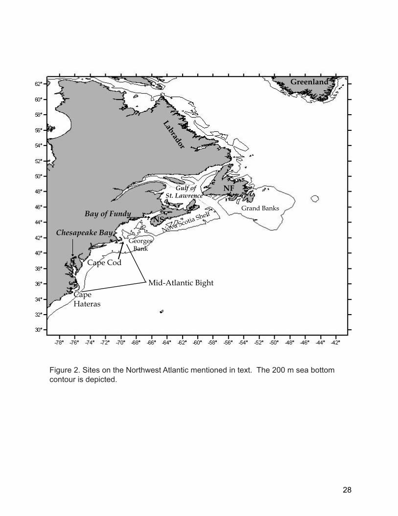
Figure 2. Sites on the Northwest Atlantic mentioned in text. The 200 m sea bottom contour is depicted.

28

New England salmon populations The location of the maximum temperature limit of Atlantic salmon (20.6°C) will

shift northward near Cape Cod and Georges Bank (Figure 3). SSTs in this region will exceed the salmon’s temperature range, presenting a barrier to adults of New England populations returning to fresh water in the summer and early fall to spawn. These fish may experience similar conditions when migrating through Scotian Shelf waters (see below). Migrating adults may be able to adapt to the changing thermal environment by migrating earlier or later in the year (Narayanan et al. 1995), but this could have adverse effects on spawning success.

Smolts emigrate from fresh water to the sea in late spring and summer (Hansen and Quinn 1998). It seems logical that warmer temperatures in these southern waters would not be a barrier to smolts emigrating from adjacent rivers and estuaries, as either emigration is too early for these critical temperatures, or if later, smolts already are acclimatized to warm water from their rivers and estuaries. However, Friedland et al. (2003) speculated that since spring air temperatures in the Gulf of Maine have increased over the past century, smolt emigrations, which are cued partly by temperature, may be earlier in the year. Earlier emigrations may be decoupled from the timing of oceanographic conditions to which Gulf of Maine salmon have adapted, affecting survival. Continued warming would exacerbate this situation. Should post-smolts attempt to avoid undesirable temperatures during marine migration, they must swim harder or further and may develop energy deficits (Friedland 1998).

Nova Scotia salmon populations outside the Bay of Fundy

The location of the maximum temperature limit for salmon in August also will shift northward on the Scotian Shelf (Figure 3). SSTs in this region will exceed the salmon’s temperature range, presenting a barrier to migrating adults of Nova Scotia (and New England) salmon populations returning from the Grand Bank or more northern waters to spawn. Because salmon populations follow hereditary migration routes and timetables (Atlantic Salmon Federation 2004), it is questionable whether returning salmon will be able to alter them and spawn successfully. However, Narayanan et al. (1995) suggested that adults can shift their migration period and route if necessary. If post-smolts swim through the warmer Scotian Shelf offshore waters during their northward migration, they will be acclimatized to cooler marine temperatures. Thus, warmer Scotian Shelf waters will be a barrier during their seaward migration. Whether these post-smolts will alter their seaward migration routes or timing to avoid warmer SSTs is open to question. Yet if migration routes are altered, the extra swimming may create energy deficits (Friedland 1998).

As in the Gulf of Maine, increasing spring air temperatures in Nova Scotia waters over the past century may have caused smolts to emigrate from fresh water earlier in the year, with consequent phenological shifts in conditions to which Nova Scotia salmon have adapted (Friedland et al. 2003). Continued warming would exacerbate this situation. Most eastern shore Nova Scotia rivers have been impacted by acid precipitation (Ritter 2000). Warming of Scotian Shelf waters would be an additional stressor to salmon originating in Nova Scotia rivers.

29

CCCma

CCSR

CSIRO

GFDL

Scenario A2 Scenario B2Model

Figure 3. Changes predicted in the thermal range of the Atlantic salmon (Salmosalar) on the Northwest Atlantic as a result of sea surface temperature changes expected to accompany a 2°C global average increase in surface air temperature projected by four AOGCMs through the A2 and B2 scenarios. Red indicates loss of thermal range, green increase, and blue no change. Cross-hatching indicates the species’ modern distribution.

30

Inner Bay of Fundy salmon populations Inner Bay of Fundy salmon populations have experienced significant decline

since 1989, primarily due to reduced marine survival (Amiro 2003). During their marine phase iBoF salmon appear to remain in Bay of Fundy,

northern Gulf of Maine, and local marine waters (Gross and Robertson 2005 MS). The marine distribution of iBoF salmon should not be affected by climate-induced warming in Cape Cod and Georges Bank waters (Figure 3), as critical SST maxima occur south of apparent post-smolt and adult migration routes and marine range. This is in contrast to outcomes suggested by the National Recovery Team (2002), whereby migration routes may be altered and survival depressed.

Should the traditional marine range of iBoF populations include Scotian Shelf waters (Amiro et al. 2003), salmon may be able to shift their distribution to avoid the higher temperatures and still find suitable habitat. Narayanan et al. (1995) found evidence for such shifts in inshore Newfoundland waters in response to cold water temperatures. Alternatively, iBoF salmon may have warmer temperature preferences than salmon elsewhere in the North Atlantic (Amiro et al. 2003), reducing the impact of warming SSTs over the Scotian Shelf.

Climate change is expected to have important indirect effects on iBoF salmon populations. Smolt emigrations into salt water may happen earlier in the year, decoupling from the timing of oceanographic conditions and impacting survival, as in other populations. Other negative impacts are predicted from their local and southern marine distribution (Irvine 2004). Marine survival will be reduced through food chain effects and increased competition and predation due to northward shifts in the distribution of warm water species. Freshwater survival will be reduced through possible adult migration delays due to reduced flows and increased temperatures, decreased spawning success because of increased sedimentation or scouring, and lower growth in summer because of poorer feeding conditions from increased summer temperatures and reduced flows.

Gulf of St. Lawrence salmon populations

Southern Gulf of St. Lawrence waters are relatively warm for the Canadian Atlantic, making them sensitive to climate change. We predict that August maximum SSTs in these waters will exceed critical values for Atlantic salmon in transit there (Figure 3). The southern Gulf drains some of Canada’s most important Atlantic salmon rivers: the Miramichi, Kouchibouguac, Kouchibouguacis, Richibucto, Buctouche, Cocagne, and Shediac. The higher temperatures will be a significant barrier to migrating adults, blocking access to these rivers for spawning. It seems reasonable that increased SSTs will not be a barrier to smolts leaving fresh water, as in New England populations. However, the timing of smolts emigrating into the Gulf of St. Lawrence appears relatively unchanged over the past century, though spring water temperatures have been warming (Friedland et al. 2003). These authors found the warmer spring temperatures were associated with poorer salmon survival, apparently due to phenological shifts during first entry into salt water. Global warming would worsen the effect.

Dutil and Coutu (1988) found many post-smolts in nearshore waters of the northern Gulf of St. Lawrence from late summer to early fall at SSTs less than 20oC. Juvenile salmon may utilize parts of the northern Gulf as a nursery area (F. Whoriskey,

31

pers. comm.). We estimate that August maxima for the northern Gulf will not exceed the critical maximum of 20.6oC (Chapter 1, Figures 1 and 3), thus the presence of post-smolts there should be unaffected. Various salmon populations

The tail of the Grand Bank is another location where the critical August maximum shifted northward (Figure 3), which will create a barrier of warmer water to the migration of post-smolts or adults moving to or from the Labrador Sea or western Greenland waters. Some Atlantic salmon spend their marine phase on the tail of the Grand Bank, and may be able to shift their distribution to avoid the higher temperatures and still find suitable habitat. Economic impacts

We conclude that the temperature regime shifts predicted may affect all aspects of the marine phase of Atlantic salmon – post-smolt migration, feeding and growth, competition for resources or predation, adult spawning migration, and ultimately survival of individuals and populations. There likely will be no impact on commercial salmon fisheries as they are closed throughout the western North Atlantic and have little chance of reopening in the coming decades. Climate change impacts on the fish probably will preclude recovery of the stocks to levels supporting commercial fisheries. However, the freshwater recreational salmon fishery is very important in Canada, and could be impacted to varying degrees. A warming climate will result in more frequent temporary closures of rivers to fishing due to warm water temperatures (Dempson et al. 2001). The famous fisheries of the rivers entering the southern Gulf of St. Lawrence may be most affected, both in terms of river closures and overly warm marine waters impacting post-smolt survival or blocking adult migrations.

A warming climate may benefit aquaculture at the expense of wild iBoF salmon populations (Irvine 2004). Should winter water temperatures rise by 1-2oC salmon aquaculture may be able to expand into waters of northern Nova Scotia, southern Newfoundland, and the Gulf of St. Lawrence (Frank et al. 1990) where the latter is not too warm in summer (Page and Robinson 1997, this study). Page and Robinson (1997) and Milewski (2002) summarized oceanographic variables having potential impact on salmon aquaculture with global warming.

The temperature regime shifts we foresee likely will seriously hinder attempts at the recovery of endangered Atlantic salmon populations, and the restoration of historic salmon runs where populations have been extirpated.

32

Summary Atlantic salmon are in serious decline through much of their range. A 2°C rise in

global temperature may exacerbate the decline as warming waters cause loss of favourable thermal habitat in the southern part of the range and no northward gain. These shifts in the temperature regime may affect all aspects of the marine phase of Atlantic salmon. Warmer waters will become barriers to migration of adults or smolts of southern populations. Smolt emigration into salt water may occur earlier in the year, impacting survival through phenological shifts. Most North American salmon populations spend their marine phase in the cold waters of the Labrador Sea, off western Greenland, or on or near the Grand Bank. A cooling trend is expected in these waters under a 2°C rise in global temperature, thus favourable marine thermal habitat for Atlantic salmon may actually decrease.

Climate change impacts on Atlantic salmon probably will preclude recovery of the stocks to levels supporting commercial fisheries. The important freshwater recreational salmon fishery will see more frequent temporary closures of rivers to fishing due to warm water temperatures, especially in the rivers entering the southern Gulf of St. Lawrence, or because of fewer fish. A warming climate may benefit aquaculture, with expansion into waters of northern Nova Scotia, southern Newfoundland, and the Gulf of St. Lawrence. Attempts at salmon recovery or restoration will be seriously hindered by warming temperatures.

Although the impacts of climate change on the freshwater phase of Atlantic salmon were not assessed in our analysis, a review of the literature revealed great vulnerability, especially in southern populations now experiencing near lethal thermal conditions in summer.

33

Atlantic deep-sea scallop, Placopecten magellanicus Background

The Atlantic deep-sea scallop is a benthic bivalve mollusc found in continental shelf waters of the western North Atlantic from Labrador to Cape Hatteras, North Carolina (Pohle et al. 2004). North of Cape Cod this species typically lives in depths less than 20 m, while south of the Cape these scallops usually are found from 40 to 200 m (Hart 2001), primarily due to temperature variation with depth (Bourne 1965).

Spawning begins in late spring further south, and occurs from late summer to early fall in more northern waters (Hart 2001). Scallops within a bed usually spawn synchronously, in a short period of time, and are triggered by a rapid temperature change, the presence of sperm from other scallops, agitation, or tides (Packer et al. 1999). Spawning in a Gulf of St. Lawrence population was found to be associated with the downwelling of warm surface water into which gametes were shed. The warm water would be favourable to larval development (Bonardelli et al. 1996). After fertilization, the eggs probably rest on the sea bottom until hatching (Packer et al. 1999). Larvae are planktonic and remain in the water column for four to eight weeks before settling to the bottom as spat (Hart 2001).

Scallops often occur in dense beds, either of a temporary nature, perhaps lasting a few years, to virtually permanent (Packer et al. 1999). Scallops do not migrate great distances, but undergo localized and random or current-assisted movement (Packer et al. 1999). Fishery Management

The Atlantic deep-sea scallop comprises one of the major invertebrate fisheries in the western North Atlantic. There are inshore fisheries in the Gulf of St. Lawrence and the Bay of Fundy off Digby, Nova Scotia, and a considerably larger offshore fishery on Georges Bank off the southwestern tip of Nova Scotia. Scallops also are fished in the Mid-Atlantic Bight, with landings recorded as far south as North Carolina (NOAA 2004). Halpin (2005) said of the fishery “Overall, US management has made recent progress towards goals of sustainability in the scallop fishery, especially through the use of closed and rotational areas. However, high fishing mortality in the Mid-Atlantic indicates that management still has significant challenges. Although Canada has been criticized as being slow to respond to scientific recommendations for conservation, in general it has managed its fishery more effectively and conservatively than the United States.”

There is growing interest in both Canada and the U.S. in cultivating scallops (Milewski 2002). Current marine temperature limits

SSTs within the scallop’s current distribution range from a February minimum of -2.1oC to an August maximum of 28.1oC. Because scallops do not migrate, they experience these temperatures in the northern and southern limits respectively of their range.

34

Relationship of SST to the benthic life style of scallops Juvenile and adult scallops are benthic and live in waters of varying vertical

thermal gradients. Thus, SSTs may not correlate with sea bottom temperatures, and predicting future sea bottom temperatures following global warming is beyond the scope of this study. For these reasons, scallops may seem an unusual species to examine with respect to climate change and warming SSTs. However, scallop abundance has been linked to the retention of their planktonic larvae in nearby waters, where temperature plays a major role in larval survival (Frank et al. 1990, Tremblay and Sinclair 1986). Therefore, at the macro-scale of our study, adult scallops will not occur where SSTs are unsuitable for their planktonic larvae. Impacts of 2oC warming on scallop distribution

The current and predicted distributions of scallops are presented in Figure 4. If SST were the sole factor controlling distribution, scallops now could exist further north (blue in Figure 4) and south (red in Figure 4 of their present range. Therefore, other factors must be restricting scallops to their present range.

A 2°C rise in global temperature will impact future distributions of scallops in western North Atlantic waters. Results from all models and scenarios are similar, and show potential loss of habitat in the southernmost part of the current range, in the vicinity of Cape Hatteras and perhaps Virginia waters depending upon the model (Figure 4). There was no northward gain of habitat in our study. The predicted loss of habitat is due to a shift northward of the August maximum currently experienced by scallops at their southern limit.

The loss of favourable thermal habitat for scallops in the southernmost part of their range may eradicate scallop beds in those waters and the small fisheries of the southern states. Likely there would be ecological ramifications resulting from scallop extinction there, as well.

Other impacts of climate change

Though we focussed on shifts in scallop distribution with global warming and the consequences, there likely will be other effects on scallops as temperatures change throughout their range. Information on the effect of environmental variables on growth, survival, and production on scallops is limited (Packer et al. 1999), and there is little information on the impact of climate change on scallops. Temperature and ocean circulation

It has been hypothesized that global warming may result in either warming or cooling of the bottom waters along the outer shelf of the Mid-Atlantic Bight, with differing implications for scallops: cooling should contribute to an increase in their distribution and productivity, and warming to a decrease (Mountain 2001).

Relatively higher water temperatures during planktonic stages of scallops have been related to improved abundance of adults in the Bay of Fundy due to good spat settlement. The higher temperatures increase the rate of larval development and thus survival, as Bonardelli et al. 1996 also noted in the Gulf of St. Lawrence, and are associated with lower exchange with outside waters, improving larval retention (Frank et al. 1990 and references therein). Likewise, Tremblay and Sinclair (1986) noted that most

35

36

Bay of Fundy scallop larvae either remain in or return to the area of major spawning. Thus scallops living in waters undergoing warming (Chapter 1, Figure 3) should experience increased abundance, while abundance in cooling waters may decline, in contrast to Mountain’s (2001) speculation for the Mid-Atlantic Bight. Posgay (1950, in Hart and Chute 2004) found that good year classes on Georges Bank were associated with tight circulation gyres in the fall because of larval retention; poorer year classes were associated with loose gyres. Oceanic circulation may be impacted by climate change in various ways. Long-term changes to the gyres on Georges Bank, Bay of Fundy, and elsewhere may reduce larval retention and thus scallop abundance. Changing circulation patterns could result in a decrease in flushing in coastal waters, leading to reduced oxygen levels and food availability for scallops.

Expansion of competitive species

Scallop larvae are very fragile when they settle to the sea bottom as spat, and for a period of time afterward. This time period is important in the formation of scallop beds and in determining year class size (Hart and Chute 2004, Packer et al. 1999 and references therein), as well as in scallop aquaculture. Successful spat settlement and survival in aquaculture and in the wild may be negatively impacted by climate-induced changes in the competing biofouling community. Potential spat competitors may undergo range extensions to overlap that of scallops, and existing competitors may see reproductive increases, all due to increased water temperatures (Robinson and Martin 2002). Kingzett (2000) raised the potential for increased invasion or colonization of shellfish grown in culture systems by exotic species as a consequence of climate change. This spectre may become a concern for the cultured scallop industry in Canada and the U.S.

37

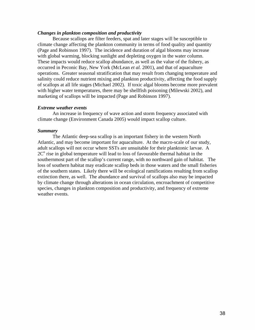
Changes in plankton composition and productivity Because scallops are filter feeders, spat and later stages will be susceptible to

climate change affecting the plankton community in terms of food quality and quantity (Page and Robinson 1997). The incidence and duration of algal blooms may increase with global warming, blocking sunlight and depleting oxygen in the water column. These impacts would reduce scallop abundance, as well as the value of the fishery, as occurred in Peconic Bay, New York (McLean et al. 2001), and that of aquaculture operations. Greater seasonal stratification that may result from changing temperature and salinity could reduce nutrient mixing and plankton productivity, affecting the food supply of scallops at all life stages (Michael 2002). If toxic algal blooms become more prevalent with higher water temperatures, there may be shellfish poisoning (Milewski 2002), and marketing of scallops will be impacted (Page and Robinson 1997).

Extreme weather events

An increase in frequency of wave action and storm frequency associated with climate change (Environment Canada 2005) would impact scallop culture. Summary

The Atlantic deep-sea scallop is an important fishery in the western North Atlantic, and may become important for aquaculture. At the macro-scale of our study, adult scallops will not occur where SSTs are unsuitable for their planktonic larvae. A 2Co rise in global temperature will lead to loss of favourable thermal habitat in the southernmost part of the scallop’s current range, with no northward gain of habitat. The loss of southern habitat may eradicate scallop beds in those waters and the small fisheries of the southern states. Likely there will be ecological ramifications resulting from scallop extinction there, as well. The abundance and survival of scallops also may be impacted by climate change through alterations in ocean circulation, encroachment of competitive species, changes in plankton composition and productivity, and frequency of extreme weather events.

38

Asian shore crab, Hemigrapsus sanguineus Background

The brachyuran crab Hemigrapsus sanguineus (de Haan 1853), also known under the common names Asiatic, Asian or Japanese shore crab, is native to the western Pacific, from Sakhalin Island (Russia) in the north, to Hong Kong and Taiwan in the south, and throughout the Japanese archipelago (Sakai 1976, McDermott 1998a). This crab has recently been introduced to areas of both sides of the Atlantic (Breton et al. 2002, Schubart 2003, Campbell and Nijland 2004). In the northwest Atlantic, it was first reported near Cape May, New Jersey in 1988 (Williams and McDermott 1990), and has since spread rapidly south to northern North Carolina and north to central Maine (Nizinski 2003). Breeding populations are now well established within the northwest Atlantic range (McDermott 1991, 1998b, 1999a), with extremely high densities of up to 150 individuals per m2 reported (Brousseau and Baglivo 2005). Primary factors contributing to the success of this invasive species are the differing pattern and lack of restriction in resource use, and the physical and climatological similarities between native and invaded regions (Lohrer et al. 2000a).

It is generally believed that the introduction, rapid dispersal and settlement of H. sanguineus was through the larval planktonic phase of this adult benthic crab. The six-stage larval phase (Kurata 1968, Hwang et al. 1993) has a duration of 16-25 days depending on temperature (Epifanio et al. 1998). This, and a tolerance to a wide range of salinities, would allow survival of long distance inter-ocean transport in ship ballast waters (Carlton and Geller 1993). Beyond the initial human-mediated introduction, the rapid and widespread dispersal from the areas of introduction may also be mediated through larval dispersal. However, the highly mobile nature and low site fidelity of the benthic adult phase of this crab (Brousseau et al. 2002) are other likely contributing factors.

Temperature limits and consequences

Given its recent introduction and potential effects on prey species, some of which are harvested for human consumption, there is considerable interest in understanding impacts (Lohrer and Whitlatch 2002a) and predicting future range increases of the Asian shore crab (Stephensen 2004). One of the principal factors that determine distribution is environmental temperature (Takahashi et al. 1985).

Based on the minimum and maximum SST’s of 0.6 and 26.1°C within its existing distribution, it is likely that the geographic range of H. sanguineus will expand along the northern coast, even in the absence of climate change. As indicated by the blue areas on maps of all models and scenarios (Figure 5), H. sanguineus should spread to southern Nova Scotia as well as the Bay of Fundy. These areas also include rocky shore habitats and prey preferred by the Asian shore crab, making such a geographic expansion likely. An analysis of relative abundance and crab sizes at different sites in New England also suggest a northward range expansion of this crab (Ledesma and O’Connor 2001).

39

Relationship of SST to temperatures experienced by crabs The temperatures experienced by the Asian shore crab are likely not strictly

equivalent to SST’s within a given area. However, while juvenile and adult crabs can be exposed to air rather than water temperatures in the intertidal zone, the two regimes tend to covary (Menne, 2000) and crabs can seek moderating shelter above or below water as necessary. Also, the planktonic larval phase of the crab occurs in waters close to the surface and therefore should experience temperatures similar to SSTs.

Implications of 2°C warming

A 2Co rise in global temperature suggests dramatic changes in the geographic distribution of the Asian shore crab. All models show a loss in the southern range (red in Figure 5) that includes Chesapeake Bay and areas that are immediately adjacent.

An extensive northern range extension is predicted by three of four models, which indicate H. sanguineus occurring throughout the coast of Nova Scotia, Gulf of St. Lawrence and parts of Newfoundland and Labrador (green in Figure 5). Thus a moderate temperature increase predicts the introduction of the Asian Shore crab throughout the Canadian Atlantic.

Consequences of range expansion

The long term ecological impact of H. sanguineus to the non-native environments is presently uncertain (Lohrer et al. 2000b). However, the introduction of exotic species such as that of the Asian shore crab can have potentially harmful consequences to the ecology of the invaded environments, including effects on indigenous species populations that may also be of commercial importance. At this point the relatively small Asian shore crab (common carapace length 3 cm) has no direct importance to humans in that it is not harvested for commercial purposes. However, there are indirect consequences. Important considerations of possible consequences primarily involve the interaction of H. sanguineus with other species.

Impacts on prey species

The Asian shore crab is considered an opportunistic omnivore (McDermott, 1999b, Ledesma and O’Connor 2001) that can survive on a diverse diet of plants, including macroalgae and salt marsh grasses, and animals, consisting of polychaetes, amphipods, barnacles, molluscs. However, when given a choice, the crab has a strong preference for animal food (Brousseau and Baglivo 2005). Molluscans are a favourite prey among species found in the crab habitat, with preference of bivalves (Bourdeau and O’Connor 2003). Commercial bivalve prey species include the northern quahog (Mercenaria mercenaria) and the oyster (Crassostrea virginica) (Brousseau et al. 2001). However, the primary bivalve prey species relevant in Canadian Atlantic waters would be the soft-shelled clam (Mya arenaria) and the blue mussel (Mytilus edulis), both important commercial species. Experimental evidence shows the Asian shore crab’s preference of Mya arenaria over M. edulis, but even the latter is consumed in large numbers, averaging 13 daily (Brousseau and Filipowicz 2001). While it prefers juvenile mussels, it is not so discriminating with soft-shelled clams, whose thinner shells likely present less of a challenge.

40

41

The high densities of H. sanguineus in the wild, and its effectiveness as a bivalve predator with large appetite, suggest that this crab will play an important role in restructuring of prey communities in areas of introduction (Broussseau et al. 2001) and could seriously reduce mussel and soft-shell clam populations in areas where these species co-occur (Brousseau and Filipowicz 2001).

Interaction with other predator species

However, the interaction with other similar predator species already present in the region must also be considered. In the northwest Atlantic, this includes a number of crabs (Seed 1980, Ropes 1988). In Canadian Atlantic waters the absence of significant populations of blue and mud crabs places the green crab (Carcinus maenas) as the principal competition of H. sanguineus. The green crab is another exotic crab species introduced to North America in the early 1800s that spread rapidly to encompass an area from Virginia to northern Nova Scotia. In many areas it became the most abundant crab causing ecological and economic harm (Lohrer and Whitlatch 2002a). Populations of green crabs have been reduced in areas where the Asian shore crab invaded (Casanova 2001, Lohrer and Whitlatch 2002b), primarily because of a differential in predation of newly recruited crabs. However, predation pressure on the native blue mussel has not decreased with declines of the green crab. Possible explanations include greater population densities of the Asian shore crab that make it a more important predator of juvenile mussels. Also, while overlapping intertidally, the green crab is found in a wider range of substrates and also further subtidally. This leads to the conclusion that the substitution of the green crab by the Asian shore crab has an apparent net negative influence on the shared blue mussel prey populations that may lead to population declines of this commercial shellfish (Brousseau and Baglivo 2005, Lohrer and Whitlatch 2002a). This is likely to equally apply to soft-shelled clams, whose predator-prey relationships are less well understood.

Summary

A 2°C rise in global temperature is likely to lead to the Asian shore crab retracting from its southern habitat of Chesapeake Bay and extending northward, throughout the coast of Nova Scotia, Gulf of St. Lawrence and parts of Newfoundland and Labrador. If the species should settle into their expanded range as successfully as it is doing now in its current range, we could expect high densities of the Asian shore crab throughout the entire Canadian Atlantic. Their large appetite for bivalves could impact soft-shelled clam and the blue mussel fisheries, and could also lead to considerable changes in the structure of prey and other similar predator communities in the wild.

42

General considerations of climate change on marine species Marine ecosystems are relatively resilient to changes in the environment, in part

because many species have potential for broad dispersal as larvae, and mobility in nektonic organisms as adults. But for this same reason, they are quite responsive to climate change, as evidenced by northward migrations during past fluctuations in sea temperatures. However, the rate of future climate change may overwhelm their ability to adapt (Lemmen and Warren 2004).

In the preceding analysis, we have focussed on the impact of changes in sea surface temperature on potential distributions of marine species in the Canadian Atlantic. However, the impacts of climate change on marine species are expected to be diverse, can be direct or indirect, and are sometimes compounding. In this section, we present a review of other climate change-related impacts on marine species from the literature.

Changes in water salinity

As the climate continues to warm, Arctic sea ice is expected to melt at an increasing rate; predictions for precipitation and freshwater runoff in Atlantic Canada vary, but the consensus seems to be that these will increase, especially south of Labrador (Moore et al. 1999, Shaw 2001). A reduction in salinity throughout the water column over the continental shelf may occur from melting of sea ice and greater precipitation and river runoff. These changes in salinity, accompanied by changes in temperature, may result in increased stratification of surface layers. Greater stratification will affect nutrient mixing, light availability, timing of the spring bloom, abundance of harmful algae, and frequency of hypoxic and anoxic events (Michael 2002, Mountain 2001).

Extreme weather events

More frequent extreme weather events are expected with global warming. Severe storm events may be more frequent (Environment Canada 2005). As in the eastern North Atlantic (Baker 2005), the Canadian Atlantic may see multiple indirect effects of weather change: increased freshwater discharge will raise coastal levels of suspended solids which can smother habitats and fish egg beds, and cause turbidity, affecting foraging of estuarine fishes and other mobile species. Greater freshwater discharge will bring more nutrients to coastal waters, causing localized eutrophication, and more pollutants. Temperature increases are likely to increase the toxicity of these chemicals. Rising sea levels and storm surges will cause loss of intertidal habitats, and spawning and nursery grounds.

Phenological mismatches

Marine pelagic communities are particularly sensitive to climate change (Edwards and Richardson 2004). Sea surface temperatures affect the timing and development of phytoplankton communities. Temperature changes may induce several oceanographic changes, influencing regional phytoplankton and zooplankton species abundance and composition and affecting the availability and suitability of prey for higher trophic levels (Frank et al. 1990, Richardson and Schoeman 2004). The level of response differs throughout the community and the seasonal cycle, leading to a mismatch between trophic levels and functional groups (Baker 2005). Such phenological shifts may affect the transfer of marine production to higher trophic levels, including commercial fishes.

43

While Edwards and Richardson (2004) anticipate a considerable climate change impact on ecosystem function in the North Sea from phenological mismatches, Schiel et al. (2004) have already seen such effects in community structure in a rocky California coastline, following seawater temperature rise resulting from a power generating station. They found benthic communities to be greatly altered in apparently cascading responses to changes in abundance of several key taxa. Community responses were mostly unpredicted in the form of direct effects on key taxa and indirect effects operating through ecological interactions. Predation

Northward range expansion of predators with increasing temperatures may impact key ecological or commercial species. In the eastern Bering Sea, the snow crab (Chionoecetes opilio) supports one of the largest crab fisheries in the world. Snow crab range has contracted to the north in the last two decades, in association with an increase in near-bottom temperature. These changes were accompanied by a northward expansion of Pacific cod (Gadus macrocephalus). The cod appear to control the southern range limit of the snow crab through predation on juveniles. Reestablishment of crab populations in the south may be hindered by cod predation, and by prevailing ocean currents which make dispersal of crab larvae to the south unlikely. Thus, recovery of lost snow crab habitat may not occur even with a reversal of the temperature regime (Orensanz et al. 2004). Disease

Climate warming can increase pathogen development, survival rates, disease transmission, host susceptibility, and range through increases in water temperature and sea level, and a decrease in salinity. The most severe disease outbreaks may occur if climate change alters host or pathogen distributions, causing formerly allopatric species to converge (Harvell et al. 2002). Eastern oyster disease is a commonly cited example of warmer temperatures encouraging the northward spread of disease. The causative organism extended its range along the east coast of the United States, from Long Island to Maine, during a winter warming trend in the mid-1980s (Harvell et al. 2002). But warmer temperatures also have been known to lead to the disappearance of disease in three species of Pacific salmonids (Holt et al. 1989). The human factor

It is expected that climate change will impact Canadian fisheries, eliminating species from all or part of their present ranges and affecting sustainable harvests; aquaculture also faces serious climate change effects (summarized by Lemmen and Warren 2004 and references therein). However, it is not easy to isolate the impacts of climate change from other stresses affecting fisheries and aquaculture. More likely, climate and non-climate related stresses, such as fishing practices, aquaculture operations, and for diadromous species, freshwater habitat destruction, dams, and irrigation facilities, will continue to compound their effects on marine ecosystems (Lemmen and Warren 2004).

44

Acknowledgements We thank Sarah Vereault and Elizabeth Flanary for producing the figures in Chapter 2. References Atlantic Salmon Federation. 2004. www.asf.ca. Amiro, P.G. 2003. Population status of inner Bay of Fundy Atlantic salmon (Salmo

salar), to 1999. Canadian Technical Report of Fisheries and Aquatic Sciences No. 2488, 39 + v p.

Amiro, P.G., J.Gibson, and K. Drinkwater. 2003. Identification and exploration of some methods for designation of critical habitat for survival and recovery of inner Bay of Fundy Atlantic salmon (Salmo salar). Department of Fisheries & Oceans CSAS Research Document 2003/120, 25 p.

Baker, T. 2005. Vulnerability assessment of the north-east Atlantic shelf marine ecoregion to climate change. World Wildlife Fund. www.wwf.org.uk/filelibrary/pdf/climatechangeandseas01.pdf.

Bonardelli, J.C., J.H. Himmelman, and K. Drinkwater. 1996. Relationship between giant scallop, Placopecten magellanicus, spawning and temperature fluctuations during downwelling events. Marine Biology 124(4): 637-649.

Bourdeau, P.E., and N.J. O’Connor. 2003. Predation by the nonindigenous Asian shore crab Hemigrapsus sanguineus. Northeastern Naturalist 10(3): 319-334.

Bourne, N. 1965. A comparison of catches by 3- and 4-inch rings on offshore scallop drags. Journal of the Fisheries Research Board of Canada 22: 313-333.

Breau, C. 2004. The effects of high water temperatures on the ecophysiology and the behaviour of juvenile Atlantic salmon (Salmo salar). Proceedings of climate change impacts and adaptation: water resources and fisheries in New Brunswick. Moncton, New Brunswick, 15-16 March 2004.

Breton, G., M. Faasse, P. Noël, and T. Vincent. 2002. A new alien crab in Europe: Hemigrapsus sanguineus (Decapoda: Brachyura: Grapsidae). Journal of Crustacean Biology 22(1):184-189.

Brousseau, D.J., and J.A. Baglivo. 2005. Laboratory investigations of food selection by the Asian shore crab Hemigrapsus sanguineus: algal versus animal preference. Journal of Crustacean Biology 25(1):130-134.

Brousseau, D.J., J.A. Baglivo, A. Filipowicz, L. Sego, and C. Alt. 2002. An experimental field study of site fidelity and mobility in the Asian Shore crab, Hemigrapsus sanguinensis. Northeastern Naturalist 9(4):381-390.

Brousseau, D.J., and A. Filipowicz. 2001. A theoretical estimate of the potential impact of Asian shore crab predation on mussel settlement. Journal of Shellfish Research 20(1):514.

Brousseau, D.J., A. Filipowicz, and J.A. Baglivo. 2001. Laboratory investigations of the effects of predator sex and size on prey selection by the Asian crab, Hemigrapsus sanguinensis. Journal of Experimental Marine Biology and Ecology 262(2):199-210.

Cairns, D.K. 2001. An evaluation of possible causes of the decline in pre-fishery abundance of North American Atlantic salmon. Canadian Technical Report of Fisheries and Aquatic Sciences No. 2358.

45

Campbell, S., and R. Nijland. 2004. De Blaasjeskrab, Hemigrapsus sanguineus, voor het eerst op het Nederlandse strand. Het Zeepaard 64(2), 40-44.

Carlton, J.T., and J.B. Geller. 1993. Ecological roulette: the global transport of non-indigenous marine organisms. Science 262:78-82.

Cassanova, T. 2001. The ecology of the Japanese shore crab (Hemigrapsus sanguineus de Haan) and its niche relationship to the green crab (Carcinus maenas Linneus) along the coast of Connecticut, USA. Proceedings of the Second International Conference on Marine Bioinvasions, pp16-17.

COSEWIC. 2005. Canadian species at risk. Committee on the Status of Endangered Wildlife in Canada. 64 pp.

Cubasch U., G.A. Meehl, G.J. Boer, M. Stouffer, M. Dix, A. Noda, C.A. Senior, S. Raper, and K.S. Yap. 2001. Projections of future climate change. Pp. 525-582 In Houghton J.T., Y. Ding, D.J. Griggs, M. Noguer, P.J. VAN DER Linden, X. Dai, K. Maskell, and C.A. Johnson (eds.). Climate change 2001: the scientific basis, contribution of working group 1 to the third assessment report of the intergovernmental panel on climate change. Cambridge University Press.

Dempson, J.B., M.F. O’Connell, and N.M. Cochrane. 2001. Potential impact of climate warming on recreational fishing opportunities for Atlantic salmon, Salmo salar L., Newfoundland, Canada. Fisheries Management and Ecology 8(1): 69-82.

Dutil, J.-D., and J.M. Coutu. 1988. Early marine life of Atlantic salmon, Salmo salar, postsmolts in the northern Gulf of St. Lawrence. Fishery Bulletin 86: 197-212.

Edwards, M., and A.J. Richardson. 2004. Impact of climate change on marine pelagic phenology and trophic mismatch. Nature 430: 881-884.

Environment Canada. 2005. The science of climate change. The Green Lane, Environment Canada's World Wide Web site. www.ec.gc.ca/climate/overview_science-e.html.

Epifanio, C.E., A.I. Dittel, S. Park, S. Schwalm, and A. Fouts. 1998. Early life history of Hemigrapsus sanguineus, a non-indigenous crab in the Middle Atlantic Bight (USA). Marine Ecology Progress Series 170: 231-238.

Frank, K.T., R.I. Perry, and K.F. Drinkwater. 1990. Predicted response of northwest Atlantic invertebrate and fish stocks to CO2-induced climate change. Transactions of the American Fisheries Society 119: 353-365.

Friedland, K. 1998. Ocean climate influences on critical Atlantic salmon (Salmo salar) life history events. Canadian Journal of Fisheries and Aquatic Sciences 55(Suppl. 1): 119-130.

Friedland, K., D.G. Reddin, J.R. McMenemy, and K.F. Drinkwater. 2003. Multidecadal trends in North American Atlantic salmon (Salmo salar) stocks and climate trends relevant to juvenile survival. Canadian Journal of Fisheries and Aquatic Sciences 60: 563-583.

Froese, R. and D. Pauly. Editors. 2005. FishBase. World Wide Web electronic publication. www.fishbase.org, version (06/2005).

Gross, M.R., and C.T. Robertson. 2005 MS. COSEWIC status report on Atlantic salmon Inner Bay of Fundy populations Salmo salar. February 28, 2005 draft report to the Committee on the Status of Endangered Wildlife in Canada. 44 p.

Halpin, P.M. 2005. Sea scallop Placopecten magellanicus. Seafood Watch Seafood Report, Monterey Bay Aquarium, 29 p. seafoodwatch.org.

46

Hansen, L.P., and T.P. Quinn. 1998. The marine phase of the Atlantic salmon (Salmo salar) life cycle, with comparisons to Pacific salmon. Canadian Journal of Fisheries and Aquatic Sciences 55(Suppl. 1): 104-118.

Hart, D. 2001. Sea scallops. In: Status of fishery resources off northeastern United States. http://www.nefsc.noaa.gov/sos/spsyn/species.html.

Hart, D.R., and A.S. Chute. 2004. Essential fish habitat source document: sea scallop, Placopecten magellanicus, life history and habitat characteristics. NOAA Technical Memorandum NMFS-NE No.189, 21 p.

Harvell, C.D., C.E. Mitchell, J.R. Ward, S. Altizer, A.P. Dobson, R.S. Ostfeld, M.D. Samuel. 2002. Climate warming and disease risks for terrestrial and marine biota. Science 296: 2158-2162.

Hofmann, E., S. Ford, E. Powell, and J. Klinck. 2001. Modeling studies of the effect of climate variability on MSX disease in eastern oyster (Crassostrea virginica) populations. Hydrobiologia 460(1-3): 195-212.

Holt, R.A., A. Amandi, J.S. Rohovec, and J.L. Fryer. 1989. Relation of water temperature to bacterial cold-water disease in coho salmon, chinook salmon, and rainbow trout. Journal of Aquatic Animal Health 1:94-101.

Hwang, S.G., C. Lee, and C.H. Kim. 1993. Complete larval development of Hemigrapsus sanguineus (Decapoda, Brachyura, Grapsidae) reared in laboratory. Korean Journal of Systematic Zoology 9:69-86.

Irvine, J. 2004. Climate Change, Adaptation, and 'Endangered' Salmon in Canada. Proceedings of the Species at Risk 2004 Pathways to Recovery Conference, March 2-6, 2004, Victoria, B.C.

Kingzett, B. 2000. Climate impacts on shellfish aquaculture in British Columbia. Workshop abstract from "Seafood Sustainability in a Changing Climate" May 25-26, 2000. www.cics.uvic.ca/workshop/FinalReport.htm.

Kurata, H. 1968. Larvae of Decapoda Brachyura of Arasaki, Sagami Bay. II Hemigrapsus sanguinensis (De Haan) (Grapsidae). Bulletin of the Tokai Regional Fisheries Research Laboratory 56: 161-165 [In Japanese, with English summary].

Ledesma, M.E. and N.J. O’Connor. 2001. Habitat and diet of the non-native crab Hemigrapsus sanguineus in southeastern New England. Northeastern Naturalist 8(1):63-78.

Lemmen, D.S., and F.J. Warren (eds.). 2004. Climate change impacts and adaptation: a Canadian perspective. Climate Change Impacts and Adaptation Directorate, Natural Resources Canada. 221 p. http://adaptation.nrcan.gc.ca/perspective_e.asp.

Lohrer, A.M., and R.B. Whitlatch. 2002a. Relative impacts of two exotic brachyuran species on blue mussel populations in Long Island Sound. Marine Ecology Progress Series 227:135-144.

Lohrer, A.M., and R.B. Whitlatch. 2002b. Interactions among aliens: apparent replacement of one exotic species by another. Ecology 83(3):719-732.

Lohrer, A.M., R.B. Whitlatch, K. Wada, and Y. Fukui. 2000a. Home and away: comparisons of resource utilization by a marine species in native and invaded habitats. Biological Invasions 2(1): 41-57.

Lohrer, A.M., R.B. Whitlatch, K. Wada, and Y. Fukui. 2000b. Using niche theory to understand invasion success: a case study of the Asian shore crab, Hemigrapsus sanguineus. Pp. 57-60 in J. Pederson, ed. Marine Bioinvasions, Proceedings of the

47

First National Conference, Jan. 24-27, 1999. MIT SeaGrant College Program, Cambridge, Massachusetts.

McCormick, S.D., R.A. Cunjak, B. Dempson, M.F. O’Dea, and J.B. Carey. 1999. Temperature-related loss of smolt characteristics in Atlantic salmon (Salmo salar) in the wild. Canadian Journal of Fisheries and Aquatic Sciences 56(9): 1649-1667.

McDermott, J. 1991. A breeding population of the western Pacific crab Hemigrapsus sanguineus (Crustacea: Decapoda: Grapsidae) established on the Atlantic coast of North America. Biological Bulletin 181: 195-198.

McDermott, J. 1998a. The western Pacific brachyuran Hemigrapsus sanguineus (Grapsidae) in its new habitat along the Atlantic coast of the United States: reproduction. Journal of Crustacean Biology 18(2):308-316.

McDermott, J. 1998b. The western Pacific brachyuran Hemigrapsus sanguineus (Grapsidae) in its new habitat along the Atlantic coast of the United States: geographic distribution and ecology. ICES Journal of Marine Science 55(2):289-298.

McDermott, J.J. 1999a. Natural history and biology of the Asian shore crab Hemigrapsus sanguinensis in the western Atlantic. Pp. 193-199. In J. Pederson, ed. Marine Bioinvasions, Proceedings of the First National Conference, Jan. 24-27, 1999. MIT SeaGrant College Program, Cambridge, Massachusetts.

McDermott, J.J. 1999b. The western pacific brachyuran (Hemigrapsus sanguineus Grapsidae) in its new habitat along the Atlantic coast of the Unites States: feeding, cheliped morphology and growth. Pp. 425-444 in F.R. Schram and J.C. von Vaupel Klein, eds. Crustaceans and the Biodiversity Crisis. Leiden, The Netherlands.

McLean, R.F., A. Tsyban, V. Burkett, J.O. Codignotto, D.L. Forbes, N. Mimura, R.J. Beamish, and V. Ittekkot. 2001. Coastal zones and marine ecosystems. Chapter 6 in Climate Change 2001: Impacts, Adaptation, and Vulnerability. Contribution of Working Group II to the Third Assessment Report of the Intergovernmental Panel on Climate Change [McCarthy, J.J., O.F. Canziani, N.A. Leary, D.J. Dokken, and K.S. White (eds.)]. Cambridge University Press, Cambridge, United Kingdom and New York, NY, USA

Menne, M. 2000. Global long-term mean land and sea surface temperatures. In: National Climatic Data Centre, Global surface temperature anomalies, http://www.ncdc.noaa.gov/oa/climate/research/anomalies/anomalies.html , p.6-8.

Michael, A. 2002. Possible effects of global warming on biological processes in the ocean. Symposium: Climate Change and Fisheries in the Gulf of Maine, Sierra Club National Marine Wildlife and Habitat Committee, April 5, 2002. www.sierraclub.org/marine/fisheries/.

Milewski, I. 2002. Climate change and salmon aquaculture in the Gulf of Maine/Bay of Fundy: Some implications. Symposium: Climate Change and Fisheries in the Gulf of Maine, Sierra Club National Marine Wildlife and Habitat Committee, April 5, 2002. www.sierraclub.org/marine/fisheries/.

Minns, C.K., R.G. Randall, E.M.P. Chadwick, J.E. Moore, and R. Green. 1995 Potential impact of climate change on the habitat and population dynamics of juvenile Atlantic salmon (Salmo salar) in eastern Canada. In: Beamish, R.J. (Ed.). Climate change and northern fish populations. Canadian Special Publcations of Fisheries and Aquatic Sciences 121: 699-708.

48

Moore, D., D. Caissie, J. Hayward, and C. Breau. 2004. Towards an understanding of the associations between adult Atlantic salmon mortalities and environmental conditions in fresh water. Proceedings, Climate change impacts and adaptation: water resources and fisheries in New Brunswick, Moncton, N.B., 15-16 March 2004.

Moore, T.R., J.A. Trofymow, B. Taylor, C.E. Prescott, C. Camire, L.C. Duchesne, J. Fyles, L. Kozak, M. Kranabetter, I.K. Morrison, M. Siltanen, C.A.S. Smith, B.D. Titus, S. Visser, R.W. Wein, and S.C. Zoltai. 1999. Litter decomposition rates in Canadian forests. Global Change Biology 5: 75-82.

Mountain, D.G. 2001. Potential Consequences of Climate Change for the Fish Resources in the Mid-Atlantic Region. American Fisheries Society symposium "Fisheries in a Changing Climate", August 2001, Phoenix, AZ.

Narayanan, S., J. Carscadden, J.B. Dempson, M.F. O’Connell, S. Prinsenberg, D.G. Reddin, and N. Shackell. 1995. Marine climate off Newfoundland and its influence on salmon (Salmo salar) and capelin (Mallotus villosus). Canadian Special Publications of Fisheries and Aquatic Sciences 121: 461-474.

National Marine Fisheries Service and U.S. Fish and Wildlife Service. 2004. Draft recovery plan for the Gulf of Maine distinct population segment of Atlantic salmon (Salmo salar). National Marine Fisheries Service, Silver Spring, MD.

National Oceanic and Atmospheric Adminstration. 2003. 3.5 Minute World Bathymetry and Topography. University of Rhode Island Environmental Data Center

National Oceanic and Atmospheric Adminstration. 2004. 2003 U.S. landings by distance from shore. www.st.nmfs.gov/st1/commercial/landings/ds_8850_bystate.html.

National Recovery Team for Inner Bay of Fundy Atlantic Salmon Populations. 2002. National Recovery Strategy for Inner Bay of Fundy Atlantic Salmon (Salmo salar) Populations. National Recovery Strategy, Recovery of Nationally Endangered Wildlife (RENEW), Ottawa. 57 pp.

Nizinski, M.S. 2003. Annotated checklist of decapod crustaceans of Atlantic coastal and continental shelf waters of the United States. Proceedings of the Biological Society of Washington 116(1):96-157.

Orensanz, J., B. Ernst, D.A. Armstrong, P. Stabeno, and P. Livingston. 2004. Contraction of the geographic range of distribution of snow crab (Chionoecetes opilio) in the eastern Bering Sea: an environmental ratchet? CalCOFI Report 45: 65-79.

Oreskes, N. 2004. The scientific consensus on climate change. Science 306: 1686. Packer, D.B., L.M. Cargnelli, S.J. Griesbach, and S.E. Shumway. 1999. Essential fish

habitat source document: sea scallop, Placopecten magellanicus, life history and habitat characteristics. NOAA Technical Memorandum NMFS-NE No.134, 21 p.

Page, F.H., and S.M.C. Robinson. 1997. Climate variability and aquaculture. In: Shaw, R.W. (Ed.). Proceedings, Climate variability and climate change in Atlantic Canada, Halifax, N.S., 3-6 December 1996. Occasional Reports of Environment Canada No. 9: 215-219

Pearson, R.G., and T.P. Dawson. 2003. Predicting the impacts of climate change on the distribution of species: are bioclimate envelope models useful? Global Ecology & Biogeography 12: 361–371.

49

Pohle, G., L. Van Guelpen, A. Martin, D. Welshman, and A. McGuire. 2004. Bay of Fundy Species Information. World Wide Web electronic publication. http://gmbis.marinebiodiversity.ca/BayOfFundy/background.html, version 1.0/2004.

Pörtner, H.O. 2002. Climate variations and the physiological basis of temperature dependent biogeography: systemic to molecular hierarchy of thermal tolerance in animals. Comparative Biochemistry and Physiology Part A 132: 739-761.

Reddin, D.G., and W.H. Shearer. 1987. Sea-surface temperature and distribution of Atlantic salmon in the northwest Atlantic Ocean. American Fisheries Society Symposium 1: 162-275.

Richardson,A.J., and D.S. Schoeman. 2004. Climate impacts on plankton ecosystems in the Northeast Atlantic. Science 305:1609-1612.

Ritter, J. 2000. The effects of acid rain on Atlantic salmon of the Southern Upland of Nova Scotia. DFO Maritimes regional habitat status report 2000/2E, 19 p.

Robinson, S.M.C., and J.D. Martin. 2002. Observations and possible future implications for biofouling in shellfish and finfish culture based on research experiences in the Bay of Fundy. Aquaculture Canada 2002 Abstracts http://www.aquacultureassociation.ca/ac02/abstracts/shellfish%20health.htm#Robinson.

Ropes, J. 1988. The food habits of five crabs at Pettaquamscutt River, Rhode Island. Fisheries Bulletin 87:197-204.

Sakai, T. 1976. Crabs of Japan and the adjacent seas. Kodansha Ltd, Tokyo, 773 pp, 251 pls.

Schiel, D.R., J.R. Steinbeck, and M.S. Foster. 2004. Ten years of induced ocean warming causes comprehensive changes in marine benthic communities. Ecology 85(7): 1833-1839.

Schubart, Ch.D. 2003. The east Asian shore crab Hemigrapsus sanguineus (Brachyura: Varunidae) in the Mediterranean Sea: an independent human-mediated introduction. Scientia Marina 67(2): 195-200.

Scott, W.B., and M.G. Scott. 1988. Atlantic fishes of Canada. Canadian Bulletin of Fisheries and Aquatic Sciences No. 219, 731 p.

Seed, R. 1980. Predator-prey relationships between the mudcrab, Panopeus herbstii, the blue crab, Callinectes sapidus, and the Atlantic ribbed mussel, Geukensia (=Modiolus) demissa. Estuarine and Coastal Shelf Science 11:455-458.

Shaw, J. 2001. The Tides of Change: Climate Change in Atlantic Canada. Geological Survey of Canada Miscellaneous Report 75.

Stephensen, E. 2004. Will the Asian shore crab, Hemigrapsus sanguineus, continue to expand its range in Maine? A thermogeographic approach to risk assessment. Northeast Ecology and Evolution Conference, Storrs, CT, USA.

Swansburg, E.O., G. Chaput, D. Caissie, and N. El-Jabi. 2004. Climate change impacts on run-timing of Atlantic salmon: adaptation of inseason models. Proceedings, Climate change impacts and adaptation: water resources and fisheries in New Brunswick, Moncton, 15-16 March 2004.

Swansburg, E.O., G. Chaput, D. Moore, D. Caissie, and N. El-Jabi. 2002. Size variability of juvenile Atlantic salmon: links to environmental conditions. Journal of Fish Biology 61(3): 661-683.

50

Swansburg, E.O., G. Chaput, N. Savoie, C. Hebert, N. El-Jabi, and D. Caissie. 2004. Proceedings, Climate change impacts and adaptation: water resources and fisheries in New Brunswick, Moncton, 15-16 March 2004.

Swansburg, E.O., E.-J. Massir, D. Caissie, and G. Chaput. 2004. Hydrometeorological trends in the Miramichi River, Canada: implications for Atlantic salmon and growth. North American Journal of Fisheries Management 24(2): 561-576.

Takahashi, K., T. Miyamoto, Y. Mizutori, and M. Ito. 1985. Ecological study on rocky-shore crabs in Oshoro Bay. Scientific Reports of the Hokkaido Fisheries Experimental Station 27:71-89 [In Japanese, with English summary].

Tremblay, M.J. and M.M. Sinclair. 1986. The horizontal distribution of larval sea scallops (Placopecten magellanicus) in the Bay of Fundy, on the Scotian Shelf and on Georges Bank. NAFO Scientific Council Research Document 86/98, 15 p.

Williams, A.B., and J.J. McDermott. 1990. An eastern United States record for the western Indo-Pacific crab, Hemigrapsus sanguineus (Crustacea: Decapoda: Grapsidae). Proceedings of the Biological Society of Washington 103:108-109.

WWF. 2001. The status of wild Atlantic salmon: a river by river assessment. World Wildlife Fund.

51

Chapter 3 Projected tree distributions, tree migration rates, and forest types in Ontario under a 2°C global temperature rise Jay R. Malcolm, Danijela Puric-Mladenovic, and Hua Shi Faculty of Forestry University of Toronto Toronto, Ontario Abstract

Using extensive information on tree populations in Ontario and the eastern United States, we applied climate, soil, topographic, and land-use information to model existing and future tree distributions in Ontario, using regression tree analysis. Based on two emissions scenarios and three General Circulation models, we calculated potential shifts in species distributions and abundances in Ontario for the period 2040-2050, at which time global temperature is expected to have risen by 2°C. Our results indicate the potential for dramatic change in Ontario's forests. The modeled climate envelopes of most species shifted significantly northward. Declines in dominance were projected in many regions for key commercial species such as black spruce, jack pine, and sugar maple. Changes in forest types were widespread as more southerly species (including species not currently found in the province) moved northwards. However, a number of factors, including fragmentation of habitat and limitations in dispersal capabilities, suggest that tree species will be unable to migrate fast enough to keep up with the enormously high migration rates that our models projected. The implication is that future ecosystem composition and function increasingly will be driven by the climatic tolerances of species, with only the more climatically tolerant species persisting at a site. Increased stress brought about by climatic conditions outside of usual climate envelopes will presumably make species more susceptible to disease and pest problems. Species may become relegated to refugia where conditions are still satisfactory.

52

Introduction In this chapter, we examine implications of a 2°C rise in global temperatures on the distributions and abundances of tree species in the central Canadian province of Ontario. We develop statistical models to relate current distributions of eastern North American tree species to climate, soil, and land-use conditions. Using these statistical (climate envelope) models, we project distributions of suitable habitats for tree species in Ontario under a 2°C global temperature rise. Disturbance regimes, such as fire and insect outbreaks, are not explicitly included in our models; these topics, as well as implications of climate change for management and biodiversity of Canadian forests are reviewed and discussed in Chapter 4. Ontario’s forests and climate change Responses of Canadian forests to climate change, and of Ontario's forests in particular, are of considerable interest in a global context. Canada is one of the largest and most heavily forested countries in the world; indeed, Canada's 400 million ha of forested and wooded lands comprise an estimated 10% of the world's forest (Natural Resources Canada 2005). The nation is one of only three on the planet where extensive areas of wilderness forests are still found (Bryant et al. 1997). At the same time, Canada is the world's largest exporter of wood products, including newsprint and softwood lumber, with the forest industry contributing some 36 billion to the nation's GDP in 2004 (Natural Resources Canada 2005). The province of Ontario in many ways provides a microcosm of the Canadian forest sector. Forests in the Province range from the heavily fragmented temperate deciduous forests of the south to the wilderness boreal forests of the far north. They comprise some 17% of Canadian forests and account for 20% of Canadian wood product exports (Natural Resources Canada 2005). Global climate models indicate that global warming will be most severe pole-ward (IPCC 2001), raising the possibility that the effects of warming will be especially pronounced in high latitude countries such as Canada. Climate is a major determinant of vegetation composition, with tree species distributions, for example, often limited to a relatively narrow range of environmental conditions (Kirschbaum 2000). As the climate changes, changes in tree distributions and their abundances are therefore projected (Woodward 1987, Loehle and LeBlanc 1996, Hansen et al. 2001, IPCC 2001, Thomas et al. 2004). Potential effects of global warming on Ontario's forests have not been analyzed quantitatively; however, indications are that they are likely to be substantial. Growing season temperature increases in the next century from the Canadian Climate Centre model are between 3 and 5° C for Ontario (Parker et al. 2000). Based on climatic requirements alone, this would imply a possible northern shift of species ranges of approximately 100-500 km (Parker et al. 2000, see also Thompson et al. 1998). In response to temperature changes of this magnitude in the past, species have shown large range shifts; indeed, temperature increases projected during the next 100 years rival those that occurred during the 10,000 years of the recent glacial retreat (McCarthy et al. 2001). In agreement with these observations, a variety of modeling efforts have indicated the potential for massive ecological change in Ontario. Based on a compilation of 14 combinations of global climate and vegetation under doubled atmospheric carbon dioxide

53

concentrations, Malcolm and Markham (2000) found that local changes in major vegetation types were expected to occur over 46% of Canada, with Ontario showing 61% change (see also Malcolm et al. 2002, Scott et al. 2002). Various other analyses similarly have shown the potential for enormous ecological change in Canada and Ontario, including changes in disturbance regimes such as fire (Suffling 1995, Stocks et al. 1998) and insect attacks (Fleming and Volney 1995), which are among the most important agents causing rapid ecosystem change (Davis and Botkin 1985, Overpeck et al. 1990, Kurz et al. 1995, Flannigan and Bergeron 1998, Thompson et al. 1998).

Because biomes do not shift as entities, but rather through responses of individual species (Delcourt and Delcourt 1988, Davis and Zabinski 1992, Webb and Bartlein 1992), models of climate change effects at the species level are especially important in understanding future ecological change. Analyses from several temperate regions again indicate the potential for massive ecosystem re-assortment. In perhaps the most comprehensive study, Iverson and Prasad (1998, 1999a, 1999b, 2001, 2002) modelled the distributions of 80 relatively common tree species in the eastern United States under recent climatic conditions (1948-1987) and under climates associated with a doubling of atmospheric carbon dioxide concentrations (as modelled by global climate models). Thirty-six species shifted their zones of maximum importance more than 100 km northward and seven were estimated to move more than 250 km. Area-weighed importances of several economically important species, such as Acer saccharum, Abies balsamea, Populus tremuloides, and Pinus resinosa, were reduced by more than 90%. Spruce-fir forests were projected to disappear from New England and maple-beech-birch forests showed near extirpation from the region. Other models of individual tree distributions in temperate regions have similarly shown large-scale range changes and extensive compositional change (Overpeck et al. 1991, Huntley et al. 1995, Sykes et al. 1996, Bartlein et al. 1997, Thompson et al. 1998, Box et al. 1999). There is now strong evidence that these and other expected ecological changes have already begun to occur under the strong warming of recent decades. In comprehensive meta-analyses of existing studies, Parmesan and Yohe (2003) and Root et al. (2003) found support for a diagnostic fingerprint of global warming responses among several hundred species across the globe. Observed responses included shifts of plant and animal species ranges on average of 6 km per decade towards the poles (or 6 metres per decade upward), shifts of breeding seasons by 2-5 days earlier per decade, and shifts in species abundances. Based on criteria defined by the Intergovernmental Panel on Climate Change, Parmesan and Yohe (2003) concluded that their analyses generated "very high confidence" that anthropogenic climate change is already affecting living systems.

54

Modeling the responses of Ontario's trees to 2° warming In this section of the report, we examine the implications of a rise of 2°C in mean global temperature for Ontario tree communities. Using extensive information on tree populations in Ontario and the eastern United States, we use climate, soil, topographic, and land-use information to model existing tree distributions in the Province. Based on two emissions scenarios for each of three General Circulation models (GCMs), we use these models to project equilibrium tree distributions and abundances in Ontario for the period 2040-2050, which lies in the middle of the period during which a 2°C global temperature rise is expected to occur (New 2005; Introduction of this report). Where a projected distribution extends beyond the current range of a species, it will only be occupied if the species can migrate fast enough to keep up with the change in environmental conditions and colonize the new part of the distribution. Therefore, following Malcolm et al. (2002), we also calculated the rates at which species might need to migrate in order to keep up with the climate change. Unlike most climate envelope approaches, which typically relate species distributions to climate alone (Box et al. 1999; Chen and Zhang 2003; Midgley et al. 2003; Thuiller 2003; Huntley et al. 2004; Skov and Svenning 2004; Svenning and Skov 2004; Thomas et al. 2004; Thuiller et al. 2004b), we include other environmental factors that may affect species distributions and abundances (e.g. soil, topography, and land-use). An additional important element of our models is our use of both Ontario and eastern U.S. data, which allowed us to model a broad north-south portion of species geographic ranges. This allowed us to model not only species that presently occur in Ontario, but also non-native species that under future climates may find suitable habitats in the Province. In total, we developed models for 130 species naturally occurring in eastern North America. Of these, 64 presently occur in Ontario whereas the rest are native to the eastern United States.

Limitations exist for this type of analysis. This method does not account for changes in physiology or for species-interactions (Iverson and Prasad, 1998). Processes such as competition and external disturbances such as fire and insect outbreaks are not included. However, this work provides a starting place for future research on how biological factors interact to produce species assemblages (Iverson and Prasad, 2002). Methods We compiled environmental data and information on tree abundances and distributions in Ontario at a spatial resolution of 300 arcseconds (approximately 7-8 km), resulting in a grid of >17,000 terrestrial cells. We used this scale because key environmental data sets were at this scale and because it approximated the 20-km scale used by Prasad and Iverson (2003; see also Prasad and Iverson 1999-ongoing), enabling us to incorporate their data into our model development. Climate and Environmental Data When possible, we calculated the same variables as Prasad and Iverson (2003; see also Iverson and Prasad 1998, 2002). To make sure that major differences did not exist between our data and theirs, we: 1) mapped the combined data and visually inspected the border area and 2) for a series of transects that traversed the border, plotted the various

55

environmental variables against latitude. When we were unable to calculate the same variables as them, we instead used global data sets and derived variables as similar as possible to theirs for both Ontario and the eastern Unites States. Recent and Future Climates.--Gridded observed climatologies for Ontario for 1961-1990 at 300 arcsecond resolution were available from McKenney et al. (2001). Future climates for 2040-2050 for the Province were available for three general circulation models (GCMs): HADCM3, CGCM2, and CSIROMk2, developed, respectively, by the U.K. Meteorological Office, the Canadian Centre for Climate Modeling and Analysis, and the Australian Commonwealth Scientific and Industrial Research Organization, respectively (Price et al. 2004, McKenney et al. 2004). These GCMs all included sulphate aerosol cooling and were used in the most recent IPCC assessment (IPCC 2001). We used the A2 and B2 emissions scenarios, which project strong regional differences in economic and population growth (A2 has stronger economic and population growth than B2; IPCC 2001). In the A2 scenario, total annual carbon dioxide emissions are projected to more than triple from the years 2000 to 2100, whereas in the B2 scenario, emissions increase by a factor of approximately 1.5 over the same time period. These projections of emissions scenarios equate to more than a doubling of carbon dioxide concentrations by the year 2100 in A2. In the B2 scenario, emissions increased by less than two times by the year 2100. For the A2 scenario, global mean temperature rise for 2040-2050 relative to 1961-1990 is 1.7º C for CSIROMk2, 1.7º C for CGCM2, and 1.5º C for HADCM3 (Figure 9.6 in IPCC 2001). For the B2 scenario, corresponding temperature increases were 1.7, 1.6, and 1.4 º C. Because of more pronounced warming towards the poles (IPCC 2001), corresponding temperature increases for Ontario were considerably higher, averaging 3.2 º, 2.4 º, and 2.1 º C for A2 and 3.1 º, 2.3 º, and 2.0 º C for B2. All scenarios projected precipitation increases relative to 1961-1990, especially in the B2 scenarios. Although nearly as warm as the A2 scenarios, the B2 scenarios were always wetter. Average percent increase in yearly precipitation for 2040-2050 in Ontario was 6.3% for CSIROMk2, 3.3% for CGCM2, and 7.6% for HADCM3 for A2; corresponding percentages were 9.2, 4.6, and 11.1% for B2. From these climate data, we calculated the same five climate variables as Iverson and Prasad (2002) and averaged them over the 2040-2050 time period (Appendix 1). Soils --Primary soil variables for Ontario and the eastern United States were available in polygon format from the Food and Agriculture Organization (FAO) Digital Soil Map of the World and secondary soil variables were available at 300-arcsecond resolution from the Global Soil Data Products CD ROM (IGBP DIS 2000). For each FAO polygon, we calculated average soil variables weighted by soil depth. Area weighted means were subsequently used to calculate soil variables in the Ontario and U.S. grid cells. From these data, we calculated a set of soil variables similar to those used by Iverson and Prasad (2002; Appendix 1). Land Use --Because of differences in land use classification between the U.S. and Ontario, we used the North America Land Cover Characteristics Data Base (Version 2.0) to derive environmental variables for both regions. This data set has a 1 km nominal spatial resolution and is based on AVHRR data spanning April 1992 to March 1993. From this data set, we used the USGS Land Use/Land Cover System map with 24 land-use classes (6 forest classes). For each grid cell in both Ontario and the USA, a fragmentation index and percent area occupied by forest, agriculture, and non forest were

56

calculated, following Iverson and Prasad (2002; Appendix 1). Digital Elevation Model (DEM) --The DEM "3D Canada" produced by the Canadian Forestry Service was used to derive topographic variables. Following Iverson and Prasad (2002), we derived maximum and minimum elevations and topographic variation within grid cells (Appendix 1). Tree data sets We combined tree abundance and distribution information from six sources: 1) a province-wide, digital Forestry Resource Inventory created by the Ontario Ministry of Natural Resources (OMNR); 2) plot-based Forest Ecological Classification data, also provided by the OMNR; 3) stand-based information collected by P.F. Maycock and his collaborators during the past 45 years; 4) tree species importance values for the eastern United States available from the USDA Forest Service (see Iverson and Prasad 2002); 5) tree distribution maps created by E. L. Little, Jr., between 1971 and 1977; and 6) AVHRR satellite data (which was used to model the abundances of three species in the northern part of the province). Methods are described in detail in Appendix 2. Species models Creating species models --For most trees species, preliminary tests indicated that the density of field plots in the grid cells was too low to accurately predicted grid-scale importance values; therefore, we modeled percent canopy dominance for common species in the FRI data set and modeled presence/absence for the rest.

We used classification and regression tree methodologies (CART) to develop the individual tree species models. This statistical technique initially splits the data set into two subsets based on a single best predictor variable. It then does the same for each of the subsets recursively (Prasad and Iverson 1998). This technique is able to form prediction rules by automatically incorporating the possibility of interactions among predictor variables (Breiman et al. 1984). One of its advantages is that it is flexible enough to capture spatial variation in driving variables (Clark and Pregibon 1992). A variety of other statistical techniques are available for this sort of modeling; indeed, authors are increasingly using several techniques in concert. We concentrated on CART here to facilitate comparisons with Iverson and Prasad (2002), who also used CART. To arrive at the dependent variable to be modeled for each species, we compare model performances for various possible dependent variables and picked the best dependent variable. For the 30 species in the FRI data set, four dependent variables were compared: 1) FRI-based canopy dominance in Ontario and IV in the United States, 2) the same, except that if Little's maps indicated that a species occurred in additional grid cells, those grid cells were assigned a low dominance value (of 1), 3) species presence/absence from the FRI, FEC, Maycock, and USDA data sets, and 4) species presence/absence from the FRI, FEC, Maycock, USDA, and Little data sets. FRI information for black spruce, jack pine, and larch included AVHRR-based predictions in the northern part of the province (see Appendix 2). We compared only models 3) and 4) for tree species not present in the FRI data set. We selected the best model based on the results of 10-fold cross-validation (Venebles and Ripley 1994; McCullough 1995; Felkner 1996; Russell 2002; Puric-Mladenovic 2003). Validation measures for canopy dominance data were

57

expressed as R2 for both training (70% of the data determined at random) and validation (the remaining 30%) data sets. Validation measures for presence/absence data were based on the area under the Receiver Operating Characteristic curve. The area is usually taken as an index of model performance because it provides a single measure of overall accuracy ranging between 0 and 1. Values greater than 0.9 indicate "excellent" discrimination, values between 0.7 and 0.9 indicate "reasonable" discrimination, and values between 0.5 and 0.7 indicate "poor to marginal" discrimination. In addition, observed and modeled distributions were overlaid onto Little's range maps and observed visually. To map predicted values (and calculate species richness values), it was necessary to define a threshold probability that indicated where a species was present. For canopy dominance, values of less than one were set to zero (absent) (Iverson and Prasad 1998). Since the default probability of 0.5 used by CART to define presence overestimated the range of some species and underestimated the range of many others (especially rare ones), for presence/absence data the optimum probability threshold value was determined based on receiver operator curve statistics (Fielding and Bell 1997; Vayssières et al. 2000; Manel et al. 2001). Models were generated using the CART algorithm in the S-plus statistical package. Future species climate envelopes and forest types --Once the species models were created, future GCM-based climate variables average over 2040-2050 were used in place of the current climate variables, and potential future species distributions were calculated. These projected future distributions indicate the location of suitable habitat for the 2040-2050 climate, based on currently-observed relationships between a species distribution and its associated climate, soil, topography, and land use conditions. This was undertaken for each GCM and each emission scenario (six scenarios in total). Species were aggregated into forest types (species assemblages) using a rule-based approach based on canopy dominances of FRI species. We used rules similar to those used to define regional "Standard Forest Units" in the Province (which are widely used in provincial forest management), but we also incorporated other information on provincial forest types and classification systems (e.g., Society of American Foresters 1940, Maycock 1963, Carleton and Taylor 1983, Hansen et al. 1992, Ontario Ministry of Natural Resources 2000). The classification had 42 forest types in total. Required migration rates – Whether or not species are be able to move in concert with shifts in their habitat conditions depends on the rate at which they would be required to migrate. Migration rates required to accompany the shifting conditions were calculated following Malcolm et al. (2002; "crow-fly" migration rates). Specifically, for each grid cell in the potential future range, the distance to the nearest grid cell in the (modeled) current distribution was calculated and then divided by the time period over which the migration occurred (55 years; i.e., 1990 to 2045). If a species was modeled to occur in a grid cell under both current and future conditions, then the migration rate for that grid cell was zero. The required migration rates were then averaged for each species across all future grid cell occurrences in the Province.

58

Results Model development Models of canopy dominance were developed for 17 FRI species, including 6 based on FRI and USDA data, 8 on FRI, USDA, and Little's data, and 3 on FRI, USDA, Little's, and NDVI-based data (Appendices 2 and 3). Over the entire study area (eastern United States and Ontario), R2 values for these species averaged 0.60 (range: 0.40-0.91) for the training data set and 0.52 (range: 0.30-0.90) for the validation data set (Appendix 3). Models of presence/absence were developed for an additional 49 species found in Ontario, including 8 models based on FRI, FEC, Maycock, and USDA data, 11 on FEC, Maycock, and USDA data, and 30 on FEC, Maycock, USDA, and Little's Ontario data (Appendices 2 and 3). Models of presence/absence for an additional 64 tree species that currently do not occur in the Province, but might in the future, also were developed. To determine if a species was likely to occur in the Province in the future, we mapped Ontario's future temperatures under present day conditions, and determined if the species ranged, at least in part, into the mapped area. To make sure that the species list was exhaustive, instead of using future climates for 2040-2050, we used future climates for 2090-2100. Area-under-the-operating-curve values for the presence/absence models averaged 0.90 ("excellent"), with only one model having a value that was less than 0.7 ("reasonable") (Appendix 3). Future climate envelopes Not surprisingly, under warmer global temperatures, the climate envelopes of most species shifted northward. This was projected to be the case for black spruce, sugar maple, jack pine, trembling aspen, and black cherry, although the exact details of the shifts varied considerably among species (Figure 1). The projected shifts sometimes were dramatic; for example, the climate envelope for black spruce moved substantially to the north in the CSIROMk2 scenario and the climate envelope of black cherry advanced far to the north in all scenarios. To investigate these shifts quantitatively, following Iverson and Prasad (1998) we defined the "latitudinal optimum" for each species as the mean latitude within the species range, weighted according to either its dominance or probability of occurrence. Strong northward shifts of these optima were seen for virtually all species under all scenarios, averaging approximately two degrees of latitude (some 230 km) for species for which canopy dominance was modeled and even more for species for which presence/absence was modeled (Figure 2). Species with especially strong shifts to the north (>3 degrees of latitude) included eastern white cedar, white spruce, blue beech, butternut, Manitoba maple, silver maple, large-toothed aspen, green ash, and red pine. In many cases, the shifts northward were into the large central land mass of the Province, hence potential species ranges in most cases also increased in size (Figure 3). Species that showed consistent decreases in potential range area were trembling aspen, balsam poplar, white birch, and black spruce.

59

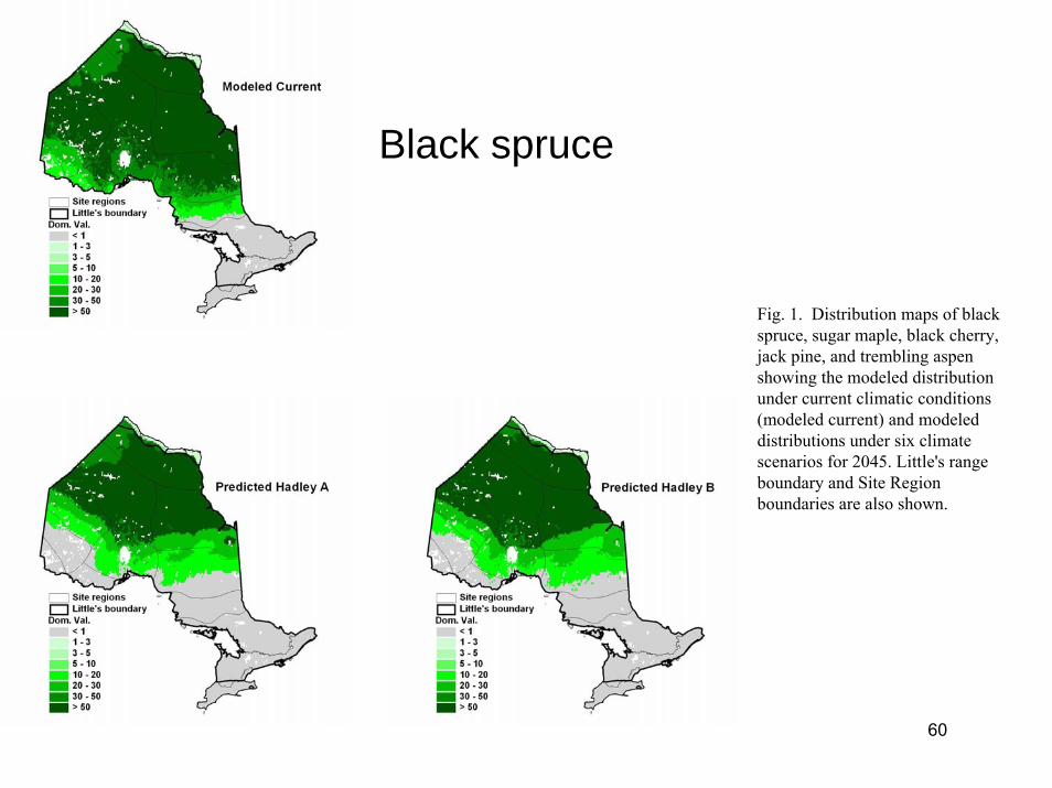
Black spruce

Fig. 1. Distribution maps of black spruce, sugar maple, black cherry, jack pine, and trembling aspen showing the modeled distribution under current climatic conditions (modeled current) and modeled distributions under six climate scenarios for 2045. Little's range boundary and Site Region boundaries are also shown.

60

61

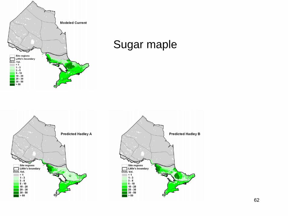
Sugar maple

62

63

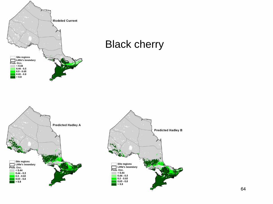
Black cherry

64

65

Jack pine

66

67

Trembling aspen

68

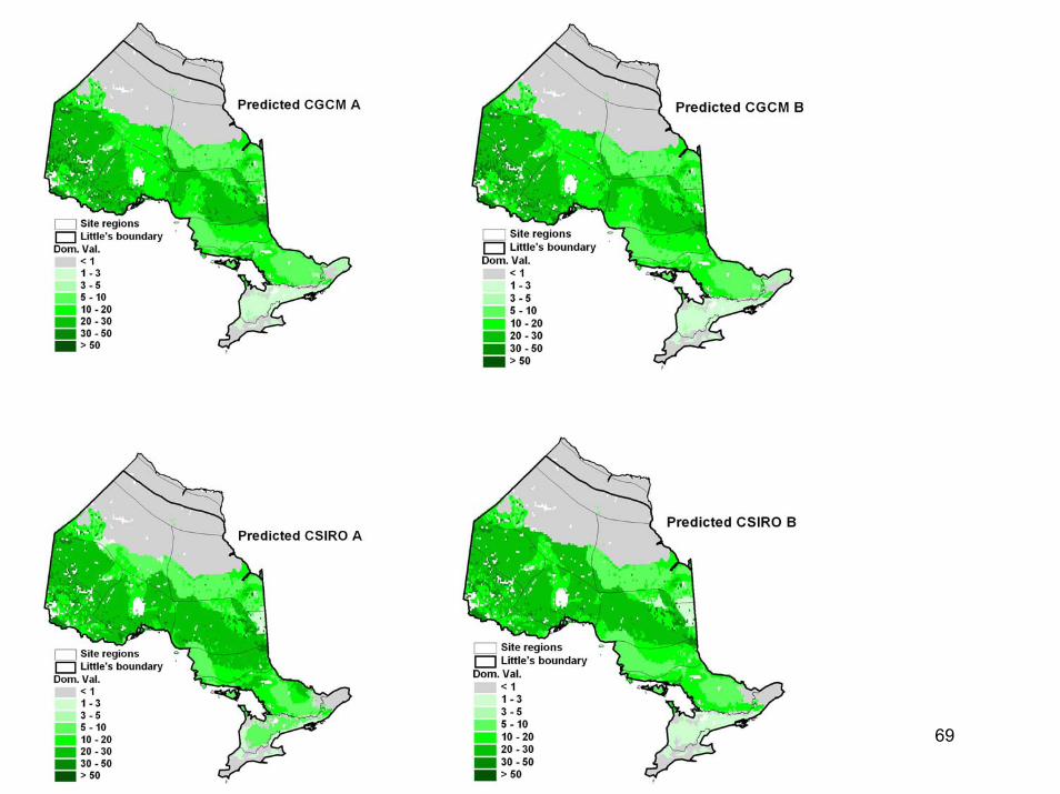
69

Current Latitudinal Optimum

42 44 46 48 50 52 5442

44

46

48

50

52

54

Futu

re L

atitu

dina

l Opt

imum

42

44

46

48

50

52

54

CGCM2-A2CGCM2-B2CSIRO-A2CSIRO-B2HADCM3-A2HADCM3-B2Y = X

Fig. 2. Species-specific future latitudinal optima for six scenarios of 2045 climates plotted against current optima for species whose canopy dominance was modeled (A) and other species currently occurring in Ontario (B). The dotted line is where Y = X.

A

B

70

Current Area (thousand km2)

0 50 100 150 200 250

0

200

400

600

800

1000

0 200 400 600 800 1000

Futu

re A

rea

(thou

sand

km

2 )

0

200

400

600

800

1000

CGCM2-A2CGCM2-B2CSIRO-A2CSIRO-B2HADCM3-A2HADCM3-B2Y = X

A

B

Fig. 3. As Fig. 2, except that future and current species distribution areas are shown.

71

Potential changes in species-specific canopy dominance Relative to current habitat conditions, future habitat conditions were such that

average dominance was projected to decline consistently across the six scenarios for nine species, including the three which currently have the highest average dominances in the Province (black spruce, sugar maple, and jack pine; Figure 4). For black spruce, average canopy dominance declined from 55 to 39-49%; for sugar maple, the decline was from 15 to 11-14%, and for jack pine, the decline was from 13 to 10-12%. Dominances increased consistently across the scenarios for four species, including the species with the next highest dominance average (trembling aspen).

Among commercially important species, the climate envelope of black spruce showed a consistent retreat northward that was most marked in the CSIROMk2 scenario (Figure 1). The climate envelope of jack pine similarly showed a shift to the northwest relative to the current climate envelope and showed reductions in southern populations especially in the eastern part of its range (Figure 1). The climate envelope of sugar maple showed a relatively slight shift northward and two of the three climate scenarios showed a marked reduction in dominance in the central part of its range east of Georgian Bay (Figure 1). The climate envelope of trembling aspen also showed an overall shift northward and a marked increase in dominance in the central part of the province (Figure 1). Potential changes in species richness Based on these equilibrium climate envelopes, species richness was more-or-less stable in the south, but increased in the northern parts of the province (Figure 5). In these northern areas, the average increase across the scenarios was by approximately five species. Required migration rates Whether or not these changes in species distributions, dominance, and richness will be realized depends in part on the rates at which climate envelopes shift relative to species capabilities. For species that currently occur in Ontario, required migration rates above and below 1,000 m/yr were about equally common, but rates below 100 m/yr and above 10,000 m/yr were rare (Figure 6). Required migration rates were much higher within Ontario for species arriving from the United States and were approximately equally distributed in the 1,000-10,000 and >10,000 m/yr classes (Figure 7). These required migration rates are averaged over the species’ entire future range: it also is of interest to ask how fast northern population fronts might move. An approximation is provided by the rate of shifts of the latitudinal optima (Figure 2). The average latitudinal shift across all species currently occurring in the province was 1.8 degrees of latitude. Since there is approximately 111 km per degree of latitude, this shift corresponds to an average required migration rate of approximately 3,600 m/yr.

These required migration rates are compared with historical migration rates in the following Discussion section.

72

Current Dominance e1 e2 e3 e4

Futu

re D

omin

ance

e0

e1

e2

e3

e4

Fig. 4. Mean canopy dominance of 17 FRI species in six scenarios of 2045 climates plotted against modeled canopy dominance under current conditions. Symbols are as in Fig. 4. The dotted line is where Y = X. 73

Mean latitude42 44 46 48 50 52 54 56

Mea

n sp

ecie

s ric

hnes

s

0

10

20

30

40

Fig. 5. Total tree species richness averaged within seven latitudinal bands. Richness is shown for current conditions (line) and for six scenarios of climates in 2045 (symbols as in Figure 4). Presence/absence of individual species was modeled using regression tree analysis. For the 17 FRI species, if modeled canopy dominance was ≥1 in a grid cell, then the species was assumed to be present. 74

Migration rate class

<100

100 -

<1,00

01,0

00 - <

10,00

0>=

10,00

0

Per

cent

of s

peci

es

0

10

20

30

40

50

60CGCM2 A2CGCM2 B2CSIROMk2 A2CSIROMk2 B2HadCM3 A2HadCM3 B2

Fig. 6. Migration rates required by species currently in Ontario to attain their modelled distributions in Ontario in 2045 Results are shown for two emissions scenarios for each of three GCMs. Rates of >1,000 m/yr have rarely been seen in the paleorecord.

75

Migration rate class

<100

100 -

<1,00

01,0

00 - <

10,00

0>=

10,00

0

Per

cent

of s

peci

es

0

20

40

60

80CGCM2 A2CGCM2 B2CSIROMk2 A2CSIROMk2 B2HadCM3 A2HadCM3 B2

Fig. 7. As Fig. 6 except that migration rates are for species that are currently absent from Ontario. Rates of >1,000 m/yr have rarely been seen in the paleorecord.

76

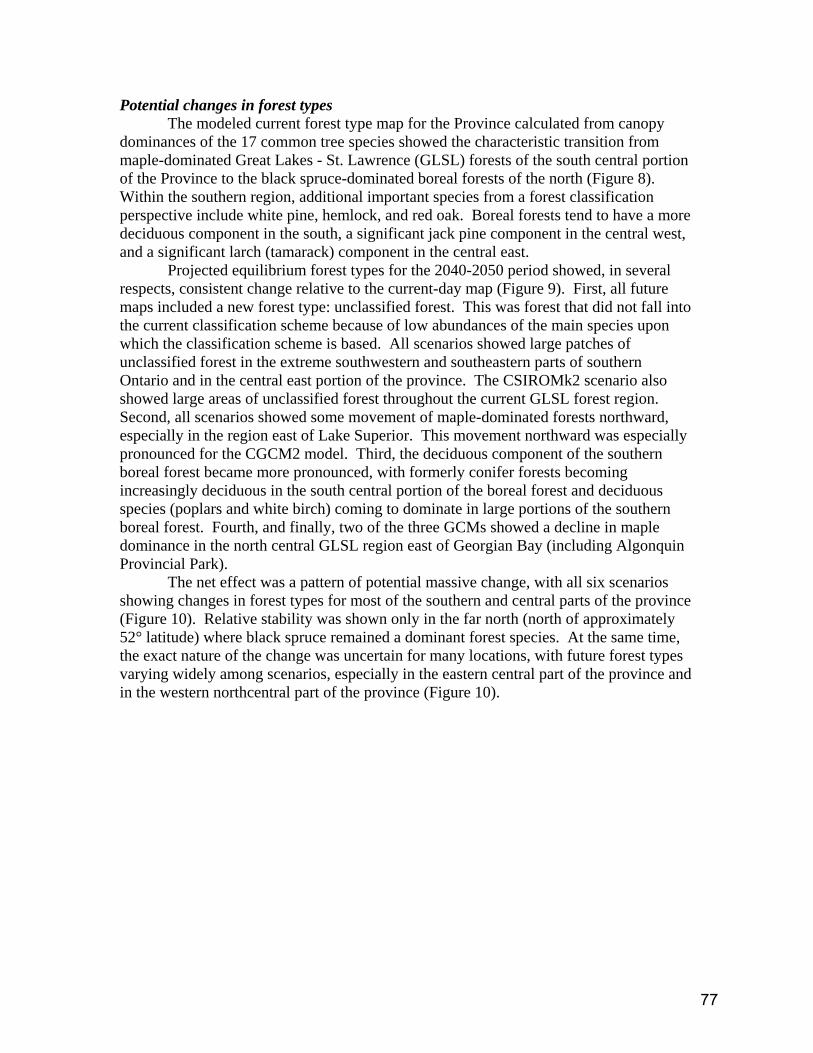
Potential changes in forest types The modeled current forest type map for the Province calculated from canopy dominances of the 17 common tree species showed the characteristic transition from maple-dominated Great Lakes - St. Lawrence (GLSL) forests of the south central portion of the Province to the black spruce-dominated boreal forests of the north (Figure 8). Within the southern region, additional important species from a forest classification perspective include white pine, hemlock, and red oak. Boreal forests tend to have a more deciduous component in the south, a significant jack pine component in the central west, and a significant larch (tamarack) component in the central east. Projected equilibrium forest types for the 2040-2050 period showed, in several respects, consistent change relative to the current-day map (Figure 9). First, all future maps included a new forest type: unclassified forest. This was forest that did not fall into the current classification scheme because of low abundances of the main species upon which the classification scheme is based. All scenarios showed large patches of unclassified forest in the extreme southwestern and southeastern parts of southern Ontario and in the central east portion of the province. The CSIROMk2 scenario also showed large areas of unclassified forest throughout the current GLSL forest region. Second, all scenarios showed some movement of maple-dominated forests northward, especially in the region east of Lake Superior. This movement northward was especially pronounced for the CGCM2 model. Third, the deciduous component of the southern boreal forest became more pronounced, with formerly conifer forests becoming increasingly deciduous in the south central portion of the boreal forest and deciduous species (poplars and white birch) coming to dominate in large portions of the southern boreal forest. Fourth, and finally, two of the three GCMs showed a decline in maple dominance in the north central GLSL region east of Georgian Bay (including Algonquin Provincial Park). The net effect was a pattern of potential massive change, with all six scenarios showing changes in forest types for most of the southern and central parts of the province (Figure 10). Relative stability was shown only in the far north (north of approximately 52° latitude) where black spruce remained a dominant forest species. At the same time, the exact nature of the change was uncertain for many locations, with future forest types varying widely among scenarios, especially in the eastern central part of the province and in the western northcentral part of the province (Figure 10).

77

Fig. 8. Modeled forest types in Ontario under current climatic conditions.

78

Fig. 9. As Fig. 8 except that projected forest types are shown for two emissions sceanrios for each of three GCMs. 79

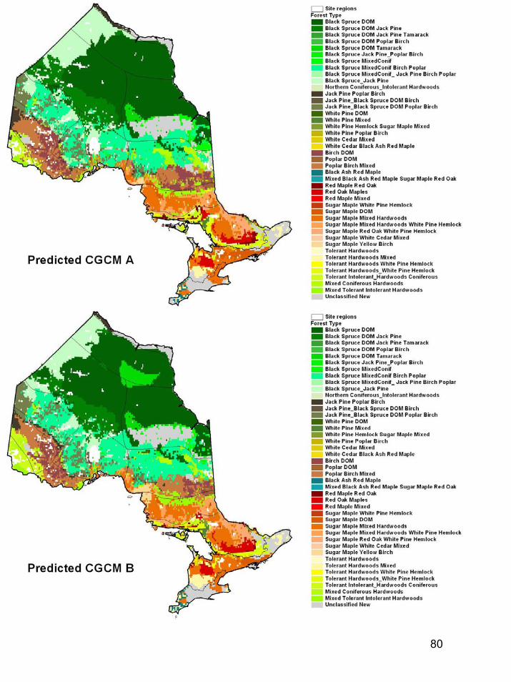
80

81

A

B

Fig. 10. Maps summarizing the overall pattern of forest type change in Ontario projected for 2045. In part A, the likelihood of forest type change is shown; namely, the number of future scenarios that showed change relative to the modeled current forest type map. In Part B, the number of forest types among the six future scenarios is shown.

82

Discussion These results indicate the potential for dramatic change in Ontario's forests under climates associated with mean global warming of approximately 2° C. By the period 2040-2050, when warming of the globe relative to baseline (1961-1990) conditions was projected to be between 1.4 and 1.7° C depending on the scenario, large shifts in species climate envelopes were projected. If species are able to follow their habitats, global warming could mean dramatic changes in tree species distributions and abundances, species richness, and forest type distributions as described by our results. If species cannot follow their habitats, ecosystem composition and function increasingly will presumably be driven by climatic tolerance, with only the more climatically tolerant species persisting at a site.

In the following sections, we begin with a discussion of the potential changes in Ontario’s forests for the case that species are able to migrate with their suitable habitats, followed by a discussion of implications for the forestry industry. We then examine the likelihood of these changes, focusing on the question of whether or not species will be able to migrate with their suitable habitats. Changes in Ontario’s forests if species migrate with their climate envelopes Although our results varied considerably among the six climate change scenarios, especially in central Ontario, some of the projected changes were consistent. First, and not surprisingly given the strong latitudinal gradient in temperature and species richness in Ontario, almost all climate envelopes showed an overall northward shift. Potential species latitudinal optima shifted northward 1.8 degrees of latitude on average, some 200 km. The shifts were more directional and pronounced than in the eastern United States, where more severe climatic change associated with doubling of carbon dioxide concentrations in five scenarios resulted in an average shift for 76 species of only 107 km (see Table 5 in Iverson and Prasad [2002]; latitudinal optima in Canada were excluded).

The implication is that for the same amount of global warming, changes to Ontario's forests will be more pronounced than further to the south. Provided that species accompany the habitat shifts, the net result of these latitudinal shifts in Ontario is a potential increase in local species richness as species of the richer southern communities move northward. A second consistent change indicated by our results was that a majority of currently-dominant species in the province showed overall declines in dominance. For species such as black spruce and jack pine, which already have their southern range limits in the province, this result is not surprising because northward moving southern range limits can be expected to result in smaller ranges in the Province and hence lower Province-wide average dominances. For others, including sugar maple, reasons for the decline are less obvious and are tied to particular changes in the combinations of climate and soil conditions required by individual species. A final consistent change was the widespread change in forest types, except in the far north where forests are projected to continue to be dominated by black spruce. In the central and southern parts the Province, almost every scenario projected changes in local forest types. In some regions, the change was consistent among scenarios: 1) large areas of unclassified forests appeared in the extreme southwestern and southeastern parts of the Province due to declines in abundances of the species that drive the classification, 2)

83

maple-dominated forests tended to move northward, especially to the region immediately east of Lake Superior, 3) shade intolerant hardwood species became increasingly abundant in the southern boreal forest, and 4) sugar maple dominance declined in the north central Great Lakes - St. Lawrence region in two of the three GCMs. Implications for forestry industry If realized, these changes could have important implications for the forest industry in the province. Several widespread, commercially-valuable species showed consistent declines in dominance, including black spruce, jack pine, and sugar maple. Given the rapid shift in climate envelopes relative to commercial rotations, the use of silvicultural systems targeted towards these species in areas of consistent range reduction is drawn into question. Under a future scenario where present-day forest management nevertheless remains in place, the potential is for an unplanned reliance on less valuable species. An example would be the planting of black spruce and jack pine in southern boreal regions where all scenarios predict climate envelope loss in a mere 40 years. What is the likelihood of these changes taking place? Whether or not these potential changes take place depends on many factors, including dispersal abilities, competition, habitat fragmentation, soil and moisture conditions, and disturbance regimes (e.g., Loehle ref.; Neilson et al. 2005; Ouranos 2004; Price et al. 2001).

The required migration rates observed here are, by historical standards (Clark 1998, McLachlan et al. 2005), enormously high. Typical rates following the glaciers during the recent glacial retreat were <500 m/yr; rates of >1,000 m/yr have rarely been observed in the paleorecord (Clark 1998). Using chloroplast DNA, McLachlan et al. (2005) concluded that species migrations were even lower than has been commonly supposed, and suggest that migration rates were typically <100 m/yr. In the simulations here, required rates of 1,000 m/yr were near the average for Ontario species, with population fronts moving on average at c. 3,400 m/yr. For invading U.S. species, rates above 10,000 m/yr were common. Although tree migration capabilities are poorly understood, even highly invasive plants are able to achieve rates of only 6,000 m/yr, raising the likelihood that many of these possibilities for migration will be unfulfilled.

Dispersal ability has been identified as a key determinant of a species’ ability to migrate (Neilson et al. 2005; Price et al 2001). Long distance migration requires transport of seed to a location far away from the existing forest boundary, followed by a build up of local breeding populations in order to establish a high likelihood of further dispersal. However, natural establishment of local breeding populations may take decades, depending on the species’ generation time. Local spread from isolated populations can occur fairly rapidly but is likely to be insufficient to keep up with the predicted climate change (Neilson et al. 2005).

Habitat fragmentation also is likely to significantly reduce migration rates (e.g., Schwartz 1992; Schwartz et al. 2001). Taking into account the current fragmented landscape, Iverson et al. (2005) estimated the likelihood of five tree species in the eastern U.S. being able to migrate into newly suitable habitats under climate change. They found that only about 5% or less of the new habitat had at least a 20% probability of being colonized over the next 100 years. There was a relatively high probability of

84

colonization within a zone 10-20 km from the current forest boundary, but the probability dropped for areas more than 20 km away. They also found that species abundance at the forest boundary was a key determinant of migration rates. Consequently, rare species may have much more difficulty in unassisted northward migration under climate change.

A final factor concerns the ability of tree species to live outside of their future climate envelopes, especially in the southern parts of ranges were distributions often are determined more by competition with other species than by climate. Provided that competitors remain absent, and depending on a species' climatic tolerance, populations may be able to persist even though climatic conditions become unsuitable (Loehle and LeBlanc 1996). Implications for Ontario’s forests

The net effect of these two factors, migration limitation and the ability of species to persist outside of their currently-observed climatic envelopes, is that at least in the short term, the composition of Ontario's forests is less likely to be driven by wholesale species turnover than by the abilities of resident populations to live outside of their climate envelopes. The likelihood is that that many species better adapted to new climates in an area will fail to arrive, with the exception perhaps of species with extremely high dispersal capabilities. If this is the case, ecosystem composition and function will presumably be driven by climatic tolerance, with only the more climatically tolerant species persisting at a site. Unfortunately, the abilities of plants to survive grow, and reproduce in climates outside of their realized niche is poorly understood (Loehle and LeBlanc 1996). Increased stress brought about by climatic conditions outside of usual climate envelopes will presumably make species more susceptible to disease and pest problems, especially for species with relatively narrow climatic tolerances, and especially in the light of likely arrivals of fast-moving populations of pests and diseases (Ayres and Lombardero 2000). Species may become relegated to refugia where conditions are still satisfactory (Iverson et al., 2005).

These results also raise serious concerns from a biodiversity viewpoint. The rapidly shifting climates observed here can be expected to be problematic for many species in Ontario, especially for those with narrow climatic tolerances, small ranges, and that occur in fragmented landcapes (Lovejoy and Hannah 2005). Many species are likely to soon find themselves outside of their typical climate envelopes. Persistence of long-lived tree despite climate changes in some cases will cause disequilibria between climatic and vegetation conditions, forcing species to "choose" between one and the other. For example, Martin (2001) found that in the face of varying climatic conditions, warbler species distributed along a moisture gradient in Arizona tended to follow climatic conditions rather than vegetation types, but incurred increased mortality when these climatic conditions did not coincide with their normal forest types. The potential for increased abundances of shade intolerant hardwoods (trembling aspen and white birch) in the southern boreal region may exacerbate an already existing problem of increased abundances of these early successional taxa in the region, despite efforts to the contrary (Hearnden et al. 1992), and the general problem of logging-induced transitions from old-growth to early successional habitats (Malcolm et al. 2004).

Some of the conclusions here apply only to forest systems with natural dispersal and migration. Human assistance, whether intentional or accidental, can accelerate the

85

migration and establishment of tree populations, although the ability to successfully promote the establishment of a wide variety of taxa is probably limited (Malcolm and Markham 2000).

Conclusion In conclusion, indications are that Ontario has the potential to undergo massive ecological change under global warming of 2º C. Previous estimates in the boreal zone have suggested that warming-induced migration rates might be an order of magnitude higher than rates estimated during the recent glacial retreat; this research raises those rates even higher. In light of the strong latitudinal gradients in species composition and forest types in Ontario and the high rates of projected climate-induced ecological change, the forest sector in Ontario may be particularly vulnerable to climate change, although confidence in future projections is hampered by a lack of information on the abilities of plant species to grow and reproduce outside of their normally-observed climatic envelopes. Silvicultural prescriptions may need to consider greater retention at stand and landscape scales to ensure margins of safety for natural regeneration. Ecological change at this rate may pose serious threats to biodiversity, especially for species that have narrow climatic tolerances and/or are adapted to particular combinations of climatic and habitat conditions. Additional risks under global climate change of 2° C include the possibility that migration will not compensate for local species losses, resulting in decreases in biomass, species richness, and consequent changes to ecological processes; increased predominance of early-successional shade intolerant species such as birch and aspen, which are already promoted by logging and other human activities; and further threats to late seral stages because of shifts in habitat conditions and resulting increased vulnerability to diseases and pests. Acknowledgements Application of the predictive tree distribution models to the 2040-50 climates was funded by World Wildlife Fund. The original creation of the predictive species models was funded by Ontario's Living Legacy Trust and the David Suzuki Foundation. Creation of the models would not have been possible without the generous contributions of time and data by team members, including Terry Carleton, Louis Iverson, Rob Kruus, Paul Maycock, Dan McKenney, Fred Pinto, Anantha Prasad, David Price, Dan Scott, and Peter Uhlig. In addition to the project team members, we also would like to thank Jim Kaputo, Travis Logan, Ken McCulloch, Sean McMurray, Larry Watkins, and Karen Zhou for their help. Helpful comments on an earlier draft of this report were made by Gaetane Boisseau, Steve Colombo, Lee Hannah, Tony Iacobelli, David Price, and Tina Tin.

86

References Ayres M. P. and Lombardero M. J. 2000. Assessing the consequences of global change

for forest disturbance from herbivores and pathogens. Science of the Total Environment 262:263-286.

Bartlein P. J., Whitlock C., and Shafter S. L. 1997. Future climate in the Yellowstone National Park region and its potential impact on vegetation. Conservation Biology 11:782-792.

Box E. O., Crumpacker D. W., and Hardin E. D. 1999. Predicted effects of climatic change on the distribution of ecologically important native tree and shrub species in Florida. Climatic Change 41:213-248.

Breiman L., Freidman J., Olshen R., and Stone C. 1984. Classification and regression trees. Wadsworth, Belmont, California, USA. 358 pp.

Bryant D., Nielsen D., and Tangley L., 1997. The Last Frontier Forests: Ecosystems and Economies on the Edge. World Resources Institute, Washington.

Carleton T. J. and Maycock P. F. 1980. Vegetation of the boreal forests south of James Bay - non-centered component analysis of the vascular flora. Ecology 61:1199-1212.

Carleton T. J., and Taylor S. J. 1983. The structure and composition of a wooded urban ravine system. Canadian Journal of Botany 61:1392-1401.

Chen X. W., Zhang X. S., and Li B. L. 2003. The possible response of life zones in China under global climate change. Global and Planetary Change 38:327-337.

Clark J. S. 1998. Why trees migrate so fast: confronting theory with dispersal biology and the paleorecord. American Naturalist 152: 204-224.

Clark J. S., Fastie C., Hurtt G., Jackson S. T., Johnson C., King G. A., Lewis M., Lynch J., Pacala S., Prentice C., Schupp E. W., Webb T., and Wyckoff P. 1998 Reid's paradox of rapid plant migration - dispersal theory and interpretation of paleoecological records. Bioscience 48: 13-24.

Clark, L. A. and Pregibon, D. 1992. Tree-based models. pp. 377-420 in JM Chambers, J Trevor and J Hastie, eds. Pacific Grove, CA: Wadsworth and Brooks/Cole Advanced Books and Software. 608 pp.

Davis M. B. and Botkin D. B. 1985. Sensitivity of cool-temperate forests and their fossil pollen record to rapid temperature change. Quaternary Research 23: 327-340.

Davis M. B. and Zabinski C. 1992. Changes in geographical range resulting from greenhouse warming: effects on biodiversity in forests. Peters, R. L. and Lovejoy, T. E. Global Warming and Biological Diversity. 297-308. New Haven, CT, Yale University Press.

Delcourt P. A. and Delcourt H. R. 1998. Paleoecological insights on conservation of biodiversity: a focus on species, ecosystems, and landscapes. Ecological Applications 8:921-934.

Felkner, J. S. 2000. A digital spatial predictive model of land-use change using economic and environmental inputs and a statistical tree classification approach: Thailand, 1970s-1990s. Ph.D. Thesis. Harvard University, Cambridge, Massachusetts. 447 pp.

Fielding, A.H.; Bell, J.F. 1997. A review of methods for the assessment of prediction errors in conservation presence/absence models. Environmental Conservation 24:38-49

Flannigan M. D., Bergeron Y., Engelmark O., and Wotton B. M. 1998. Future wildfire in circumboreal forests in relation to global warming. Journal of Vegetation Science

87

9:469-476. Fleming R. A. and Volney W. J. A. 1995. Effects of climate-change on insect defoliator

population processes in Canada boreal forest - some plausible scenarios. Water Air and Soil Pollution 82: 445-454.

Hansen, H. M; T. Frieswyk; J.F. Glover; J.F. Kelly. 1992. The Eastwide Forest Inventory Data Base: Users Manual. USDA Forest Service, GTR NC-151, North Central Forest Experiment Station.

Hansen AJ, Neilson RR, Dale VH, Flather CH, Iverson LR, Currie DJ, Shafer S, Cook R, Bartlein PJ. 2001. Global change in forests: Responses of species, communities, and biomes. Bioscience 51:765-779.

Hearnden, K.W., S.V. Millson and W.C. Wilson. 1992. A report on the status of forest regeneration. Ontario Ministry of Natural Resources, Toronto, Ont. 117 p.

Huntley B, Green RE, Collingham YC, Hill JK, Willis SG, Bartlein PJ, Cramer W, Hagemeijer WJM, Thomas CJ. 2004. The performance of models relating species geographical distributions to climate is independent of trophic level. Ecology Letters 7:417-426.

Huntley B., Berry P. M., Cramer W., and Macdonald A. P. (1995) Modelling present and potential future ranges of some European higher plants using climate response surfaces. Journal of Biogeography 22:967-1001.

IGBP-DIS. 2000. International Geosphere-Biosphere Programme, Data and Information System. Global Soil Data Task. Global Soil Data Products CD-ROM (IGBP-DIS). CD-ROM., Potsdam, Germany. Available from Oak Ridge National Laboratory Distributed Active Archive Center, Oak Ridge, Tennessee, U.S.A.

IPCC. 2001. Climate change 2001: the science of climate change. Intergovernmental Panel on Climate Change Working Group 1 Third Assessment Report. Cambridge University Press, Cambridge.

Iverson L. R. and Prasad A. M. 1998. Predicting abundance of 80 tree species following climate change in the eastern united states. Ecological Monographs 68:465-485.

Iverson L. R. and Prasad A. M. 2001. Potential changes in tree species richness and forest community types following climate change. Ecosystems 4:186-199.

Iverson L. R. and Prasad A. M. 2002. Potential redistribution of tree species habitat under five climate change scenarios in the eastern US. Forest Ecology and Management 155:205-222.

Iverson, L. R., Prasad, A. M., Hale, B. J., and Sutherland, E. K. 1999a. Atlas of currrent and potential future distributions of common trees of the eastern United States. Northeastern Research Station, General Technical Report NE-265, United States Department of Agriculture, Forest Service.

Iverson, LR, Prasad, A, Schwartz, MW. 1999b. Modeling potential future individual tree-species distributions in the eastern United States under a climate change scenario: A case study with Pinus virginiana. Ecological Modelling 115:77-93.

Iverson, L. R., A. M. Prasad, and M. W. Schwartz . 2005. Predicting potential changes in suitable habitat and distribution by 2100 for tree species of the eastern United States. Journal of Agricultural Meteorology 61:29-37.

Iverson, L. R., M. W. Schwartz, and A. Prasad. 2004. How fast and far might tree species migrate under climate change in the eastern United States? Global Ecology and Biogeography 13:209-219.

88

Joyce L. A., Mills J. R., Heath L. S., Mcguire A. D., Haynes R. W., and Birdsey R. A. 1995. Forest sector impacts from changes in forest productivity under climate change. Journal of Biogeography 22:703-713.

Kienast F, Wildi O, Brzeziecki B. 1998. Potential impacts of climate change on species richness in mountain forests - An ecological risk assessment. Biological Conservation 83:291-305.

Kirschbaum MUF. 2000. Forest growth and species distribution in a changing climate. Tree Physiology 20:309-322.

Kurz W. A., Apps M. J., Stocks B. J., and Volney W. J. 1995. Global climate change: disturbance regimes and biospheric feedbacks of temperate and boreal forests. Woodwell, G. M. and Mackenzie, F. T. Biotic Feedbacks in the Global Climate System - Will the Warming Feed the Warming? 119-133. New York, NY, Oxford University Press.

Little, E.L., Jr., 1971. Atlas of United States trees, Volume 1, Conifers and important hardwoods: Misc. Pub. 1146. Washington, D.C.: U.S. Department of Agriculture. 200 maps.

Loehle C, and LeBlanc D. 1996. Model-based assessments of climate change effects on forests: A critical review. Ecological Modeling 90:1-31.

Lovejoy T. E. and Hannah L. (eds). 2005. Climate change and biodiversity. New Haven, CT, Yale University Press, 418 p.

Malcolm J. R. and Markham A. 2000. Global Warming and Terrestrial Biodiversity Decline. Washington, DC, World Wildlife Fund.

Malcolm J. R., Markham A., Neilson R. P., and Garaci M. 2002. Estimated migration rates under scenarios of global climate change. Journal of Biogeography 29:835-849.

Malcolm, J. R., B. D. Campbell, B. G. Kuttner, and A. Sugar. 2004. Potential indicators of the impacts of forest management on wildlife habitat in northeastern Ontario: A multivariate application of wildlife habitat suitability matrices. Forestry Chronicle 80:91-106.

Manel, S.; Williams, H.C.; Ormerod, S.J. 2001. Evaluating presence-absence models in ecology: the need to account for prevalence. Journal of Applied Ecology, 38:921-931.

Martin T. E. 2001 Abiotic vs. biotic influences on habitat selection of coexisting species: Climate change impacts? Ecology 82:175-188.

Maycock. P.F. 1963. The phytosociology of the deciduous forests of extreme southern Ontario. Canadian Journal of Botany 41:379-439.

Maycock P. F. and Curtis J. T. 1960. The Phytosociology of Boreal Conifer-Hardwood Forests of the Great Lakes Region. Ecological Monographs 30:1-36.

McCarthy J. J, Canziani O. F., Leary N. A., Dokken D. J., and White K. S. (eds.) 2001. Climate Change 2001: Impacts, Adaptation, and Vulnerability (Contribution of Working Group II to the Third Assessment Report of the Intergovernmental Panel on Climate Change). Cambridge, UK, Cambridge University Press.

McCullough, P.E. 1995. Predictive vegetation mapping using classification tree analysis. Masters thesis, Dept. of Geography, San Diego State University, San Diego, CA. 177 pp.

McKenney, D.W.; Kesteven, J.L.; Hutchinson, M.F.; Venier, L. 2001. Canada's plant hardiness zones revisited using modern climate interpolation techniques. Canadian Journal of Plant Science 81:139-143.

89

McKenney, D. W., Hutchinson, M. F., Papadopol, P., and Price, D.T. 2004. Evaluation of alternative spatial models of vapour pressure in Canada. Proc. 26th Conference on Agricultural and Forest Meteorology, Vancouver, B.C., 23-26 August, 2004, 11 pp. CD-ROM.

McLachlan, J. S., J. S. Clark, and P. S. Manos. 2005. Molecular indicators of tree migration capacity under rapid climate change. Ecology 86:2088–2098.

Midgley GF, Hannah L, Millar D, Rutherford, MC, Powrie, LW. 2002. Assesing the vulnarbility of species richness to anthropogenic climate change in a biodiversity hotspots. Global Ecology and Biogeography 11:445-451.

Natural Resources Canada. 2005. The State of Canada's Forests 2004-2005: The Boreal Forest. Canadian Forest Service, Natural Resources Canada, Ottawa.

Neilson, R. P., Pitelka, Louis F., Solomon, Allen M., Nathan, Ran, Midgley, Guy F., Fragoso, Jóse M.V., Lischke, Heike, Thompson, Ken. 2005. Forecasting Regional to Global Plant Migration in Response to Climate Change. BioScience 55:749-759.

New, M. G. 2005. Arctic climate change with a 2°C global warming. In: Rosentrater, L. D., M. New, J. O. Kaplan, et al. Evidence and Implications of Dangerous Climate Change in the Arctic. Oslo, WWF: 1-15.

Ontario Ministry of Natural Resources. 2000. A Silvicultural Guide to Managing Southern Ontario Forests. Ontario Ministry of Natural resources. Queens Printer for Ontario, 422 pp.

Ouranos, 2004. S’adapter aux changements climatiques. (Campagna, Michel, Thème : La forêt, page 23). 91 pages

Overpeck J. T., Bartlein P. J., and Webb III T. 1991. Potential magnitude of future vegetation change in eastern North America: comparisons with the past. Science 254:692-695.

Overpeck J. T., Rind D., and Goldberg R. 1990. Climate-induced changes in forest disturbance and vegetation. Nature 343:51-53.

Parker W. C., Colombo S. J., Cherry M. L., Flannigan M. D., Greifenhagen S., Mcalpine R. S., Papadopol C., and Scarr T. 2000. Third Millennium forestry: what climate change might mean to forests and forest management in Ontario. Forestry Chronicle 76:445-463.

Parmesan C. and Yohe G. 2003. A globally coherent fingerprint of climate change impacts across natural systems. Nature 421:37-42.

Prasad, A. M. and L. R. Iverson. 1999-ongoing. A Climate Change Atlas for 80 Forest Tree Species of the Eastern United States [database]. http://www.fs.fed.us/ne/delaware/atlas/index.html, Northeastern Research Station, USDA Forest Service, Delaware, Ohio.

Prasad, A. M. and L. R. Iverson. 2003. Little's range and FIA importance value database for 135 eastern US tree species. http://www.fs.fed.us/ne/delaware/4153/global/littlefia/index.html, Northeastern Research Station, USDA Forest Service, Delaware, Ohio.

Price, D.T., McKenney, D.W., Caya, D, and Côté, H. 2001. Downscaled transient high resolution national climate change scenario data for Canada from 1950-2070 for seven climate variables. Canadian Forest Service and Université du Québec à Montréal.

Price, D.T., McKenney, D. W., Papadopol, P., Logan, T., and Hutchinson, M. F. 2004. High resolution future scenario climate data for North America. Proc. 26th Conference

90

on Agricultural and Forest Meteorology, Vancouver, B.C., 23-26 August, 2004, 13 pp. CD-ROM.

Puric-Mladenovic 2003. Predictive vegetation modeling for forest management and conservation in settled landscapes. Ph.D. Thesis, University of Toronto, 282 pp.

Root T. L., Price J. T., Hall K. R., Schneider S. H., Rosenzweig C., and Pounds J. A. 2003. Fingerprints of global warming on wild animals and plants. Nature 421: 57-60.

Russell, SP. 2002. Predictive soil mapping in the Mojave Desert of California. Ph.D. Thesis, University of California, Santa Barbara, 166 pp.

Schwartz M. W. 1992. Modelling effects of habitat fragmentation on the ability of trees to respond to climatic warming. Biodiversity and Conservation 2:51-61.

Schwartz MW, Iverson LR, Prasad AM. 2001. Predicting the potential future distribution of four tree species in Ohio, USA, using current habitat availability and climatic forcing. Ecosystems, 4:568-581.

Scott D., Malcolm J. R., and Lemieux C. 2002. Climate change and modelled biome representation in Canada's national park system: implications for system planning and park mandates. Global Ecology and Biogeography 11: 475-484.

Skov F, and Svenning JC . 2004. Potential impact of climatic change on the distribution of forest herbs in Europe. Ecography, 27:366-380.

Society of American Foresters, Committee on Forest Types. 1940. Forest cover types of the eastern United States; report of the Committee on forest types, Society of American foresters. Washington, D.C., Society of American foresters. 39 pp.

Stocks B. J., Fosberg M. A., Lynham T. J., Mearns L., Wotton B. M., Yang Q., Jin J. Z., Lawrence K., Hartley G. R., Mason J. A., and Mckenney D. W. 1998. Climate change and forest fire potential in Russian and Canadian boreal forests. Climatic Change 38: 1-13.

Suffling R. 1995. Can disturbance determine vegetation distribution during climate warming? A boreal test. Journal of Biogeography. 22:501-508.

Svenning JC, and Skov F. 2004. Limited filling of the potential range in European tree species. Ecology Letters 7:565-573.

Sykes M. T. and Prentice I. C. 1996. Climate change, tree species distributions and forest dynamics: a case study in the mixed conifer/northern hardwoods zone of northern Europe. Climatic Change 34:161-177.

Thomas CD, Cameron A, Green RE, Bakkenes M, Beaumont LJ, Collingham YC, Erasmus BFN, de Siqueira MF, Grainger A, Hannah L, Hughes L, Huntley B, van Jaarsveld AS, Midgley GF, Miles L, Ortega-Huerta MA, Peterson AT, Phillips OL, Williams SE. 2004. Extinction risk from climate change. Nature, 427:145-148.

Thompson I. D., Flannigan M. D., Wotton B. M., and Suffling R. 1998. The effects of climate change on landscape diversity: an example in Ontario forests. Environmental Monitoring and Assessment 49:213-233.

Thuiller W . 2003. BIOMOD - optimizing predictions of species distributions and projecting potential future shifts under global change, Global Change Biology, 9 (10): 1353-1362.

Thuiller W, Brotons L, Araujo MB, Lavorel S. 2004. Effects of restricting environmental range of data to project current and future species distributions. Ecography, 27 (2): 165-172.

Vayssières, M.P.; Plant, R.E.; Allen-Diaz, B.H. 2000. Classification trees: An

91

alternative non parametric approach for predicting species distributions. Journal of Vegetation Science, 11:679-694.

Venebles, W N, Ripley, BD. 1994. Modern applied statistics with S-PLUS. Springer-Verlag, New York, 462 pp.

Webb T. and Bartlein P. J. 1992. Global changes during the last 3 million years - climatic controls and biotic responses. Annual Review of Ecology and Systematics 23:141-173.

Woodward, FI. 1987. Climate and plant distribution. Cambridge University Press, Cambridge.

92

Appendix 1. Environmental variables used to model tree abundances and distributions in Ontario and the eastern United States. Unless otherwise indicated, data for the eastern United States was from Prasad and Iverson (2003).

Variable group Abbreviation Variable

Climate variables1 Ppt Total annual precipitation (mm)

Tavg mean annual temperature (C)

Tjan mean January temperature (C)

Tjul mean July temperature (C)

Tmaysep Mean May-Sept temperature (C)

Topographic variables2 Elv_min Minimum elevation (m)

Elv_max Maximum elevation (m)

Elv_rang Difference between maximum and minimum elevation (m)

Elv_mean Mean elevation (m)

Elv_Cv Coefficient of variation of elevation (%)

SLOPE Slope (%)

Soil variables3

FAO soil units (%) ACRISOLS Percent area dominated by Acrisols

CAMBISOLS Percent area dominated by Cambisols

CHERNNOZEM Percent area dominated by Chernozems

FLUVISOLS Percent area dominated by Fluvisols

GLEYSOLS Percent area dominated by Gleysols

GREYZEMS Percent area dominated by Greyzems

HISTOSOLS Percent area dominated by Histosols

KASTANOZEM Percent area dominated by Kastanozems

LITHOSOLS Percent area dominated by Lithosols

LUVISOLS Percent area dominated by Luvisols

NITOSOLS Percent area dominated by Nitisols

PHAEOZEMS Percent area dominated by Phaeozems

PLANOSOLS Percent area dominated by Planosols

PODZOLS Percent area dominated by Podzols

PODZOLUVIS Percent area dominated by Podzoluvisols

REGOSSOLS Percent area dominated by Regosols

93

RENDZINAS Percent area dominated by Rendzinas

SOLONCHAKS Percent area dominated by Solonchaks

SOLONETZES Percent area dominated by Solonetz

VERTISOLS Percent area dominated by Vertisols

XEROSOLS Percent area dominated by Xerosols

YERMOSOLS Percent area dominated by Yermosols

WATER Percent area dominated by Water

Secondary soil variables BULK Bulk Density (g/cm3) (0-100cm)

FIELDCAP Field Capacity (mm) (PsiFC=-10 kPa) (0-100cm)

PAWC Profile Available Water Capacity (mm) (PsiFC=-10kPa; PsiWP=-1500kPa) (0-.100cm)

SOILCARB Soil-Carbon Density (kg/m2) (0-100cm)

THERMCAP Thermal Capacity (J/m3/K) (Water Content=0.00 %v/v) (0-100cm)

TOTALN Total Nitrogen Density (g/m2) (0-100cm)

WILTPOINT Wilting-Point (mm) (PsiWP=-1500 kPa) (0-100cm)

SOIL.DEPTH Soil depth (cm)

Primary soil variables SND Percent of sand (% w/w)

SLT Percent of silt (% w/w)

CLY Percent of clay (% w/w)

PHW pH measured in water

BS base saturation (%)

Landscape pattern variables4 FRAG Fragmentation indicator

Land use/cover variables4 FOREST Percent area covered by forest

AGRICULT Percent area covered by agriculture

NONFOR Percent area covered by nonforest

1Climate normals for Ontario for 1961-1990 from McKenney et al. (2001). Future climates (averaged across 2040-2050) were from GCMs downscaled by the Natural Resources Canada, Canadian Forestry Service. 2 From Canada3D 30-arcsecond digital elevation model, Natural Resources Canada, Canadian Forestry Service, Ontario region. 3 Data for Ontario and the eastern United States derived from the Digital Soil Map of the World, V. 3.5, and the Global Soil Data Products CD ROM (International Geosphere Biosphere Programme, Data and Information System, Potsdam, Germany. Available from Oak Ridge National Laboratory Distributed Active Archive Center, Oak Ridge, Tennessee, U.S.A. [http://www.daac.ornl.gov]). 4 Data for Ontario and the eastern United states derived from North America Land Cover Characteristics Data Base, Version 2.0.

94

Appendix 2. Sources and processing of tree distributional data.

Forest Resources Inventory (FRI) Data --Digital FRI data were at two resolutions: stand-level for the central part of the province and township-level for the southern part of the province. These data provided aerial-photo-interpreted percent canopy dominance (estimated to the nearest 10%) for 30 common tree species of the Province. For stand-level data, species-specific canopy dominance was calculated within grid cells by taking the mean canopy dominance across the forested stands in the cell, weighted by the areas of the stands. For township-level data, stand-level canopy percentages and stand areas also were available, but without accompanying spatial information. Therefore, for each species we calculated mean percent canopy dominance in each township (again weighted by stand area). The 300-arc-second grid was then overlaid onto the township information and canopy percentages per grid cell calculated using area-weighted means. Forest Ecosystem Classification (FEC) data --These data were from 4,645 geo-referenced field plots of varying sizes and sampling strategies. Importance value (IV) for species x was calculated as: (1) IVx = 50·(BAx / sum of (BAx)) + 50·(NSx / sum of (NSx)) where BAx is the basal area of species x and NSx is its number of stems. IV was rounded to the nearest integer with the exception of IVs greater than zero, but less than one, which were rounded up to 1 to preserve presence/absence information (Prasad and Iverson 2002). Maycock data --We extracted information for over 800 vegetation plots from data collected by Paul F. Maycock and his collaborators over a 40 year period, including IV values as defined above. These data were collected using point-quadrant methods detailed in Maycock and Curtis (1960; see also Carleton and Maycock 1980). USDA data --Species-specific IVs at 20-km resolution (Albers Projection) for the United States east of 100° W longitude were downloaded from the United States Department of Agriculture (USDA) Forest Service web site (Prasad and Iverson 2003); see also Prasad and Iverson 1999-ongoing). Importance values were calculated as in equation (1). Little's tree distribution maps --These tree distribution maps, drawn by Elbert L. Little, Jr., between 1971 and 1977 (e.g., Little 1971) were available in digital form from the USDA Forest Service (see Iverson and Prasad 2002). AVHRR-based tree distributions --The above data sets provided little information on tree populations north of the FRI boundary, raising the possibility that distributional models might perform poorly in the northern part of the province. AVHRR satellite data, which are available on a daily timescale throughout the year, permit a large number of land cover types to be distinguished even in northern forested localities (e.g., North America Land Cover Characteristics Data Base, Version 2.0, USGS), suggesting that they might be useful in distinguishing among different tree species. The following steps were used to predict species-specific canopy dominances north of the FRI boundary from these data: 1) a training data set was created consisting of FRI-based species-specific canopy dominances for grids cells south of the FRI northern boundary and within 100 km of it; 2) for each of these grid cells, we downloaded the mean monthly NDVI values for 1-km resolution AVHRR data collected in the period April 1992 to March 1993; and 3) regression tree analysis was used to model species canopy dominances as a function of the 12 monthly NDVI values. Good fits were shown for black spruce, jack pine, and larch; therefore, for these three species we used the AVHRR-based predictions north of the FRI boundary to supplement information from the other data sets.

95

Appendix 3. Tree species modeled and model validation statistics.

R2 for validation data set

Area under the curve for receiver operating curve

validation

Species Ontario and

eastern United States

Ontario only

Ontario and eastern United

States

Ontario only

Abies balsamea 0.54 0.42 0.96 0.74

Acer barbatum 0.85

Acer negundo 0.81 0.83

Acer saccharum ssp. nigrum 0.98 0.99

Acer pensylvanicum 0.96 0.98

Acer rubrum 0.56 0.69 0.96 0.97

Acer saccharum 0.64 0.73 0.96 0.98

Acer saccharinum 0.81 0.85

Aesculus glabra 0.90

Aesculus octandra 0.90

Alnus glutinosa 0.88

Asimina triloba 0.86

Betula alleghaniensis 0.60 0.61 0.96 0.96

Betula lenta 0.93

Betula nigra 0.66

Betula papyrifera 0.67 0.66 0.94 0.66

Betula populifolia 0.96 0.98

Bumelia lanuginosa 0.89

Carpinus caroliniana 0.82 0.79

Carya aquatica 0.90

Carya cordiformis 0.83 0.93

Carya glabra 0.96 0.94

Carya illinoensis 0.89

Carya laciniosa 0.89 0.97

Carya ovata 0.87 0.98

Carya texana 0.95

Carya tomentosa 0.93

Castanea dentata 0.93 0.99

Catalpa speciosa 0.81

Celtis laevigata 0.88

Celtis occidentalis 0.90 0.85

Cercis canadensis 0.88

Chamaecyparis thyoides 0.91

Cornus florida 0.96 0.99

96

Diospyros virginiana 0.88

Fagus grandifolia 0.36 0.31 0.95 0.98

Fraxinus americana 0.93 0.94

Fraxinus nigra 0.55 0.61 0.03 0.89

Fraxinus pennsylvanica 0.79 0.88

Fraxinus quadrangulata 0.92 0.94

Gleditsia aquatica 0.89

Gleditsia triacanthos 0.90 0.95

Gordonia lasianthus 0.97

Gymnocladus dioicus 0.88 0.85

Halesia spp. 0.80

Ilex opaca 0.90

Juglans cinerea 0.81 0.88

Juglans nigra 0.93 0.95

Juniperus virginiana 0.91 0.98

Larix laricina 0.35 0.33 0.95 0.92

Liquidambar styraciflua 0.97

Liriodendron tulipifera 0.97 0.99

Maclura pomifera 0.83

Magnolia acuminata 0.87 0.74

Magnolia grandiflora 0.92

Magnolia macrophylla 0.89

Magnolia virginiana 0.95

Morus rubra 0.85 0.97

Nyssa aquatica 0.92

Nyssa sylvatica var. biflora 0.93

Nyssa ogechee 0.95

Nyssa sylvatica 0.96 1.00

Ostrya virginiana 0.85 0.93

Oxydendrum arboreum 0.96

Persea borbonia 0.94

Picea glauca 0.44 0.25 0.94 0.72

Picea mariana 0.90 0.82 0.94 0.97

Picea rubens 0.98 0.97

Pinus banksiana 0.65 0.60 0.97 0.94

Pinus clausa 0.95

Pinus echinata 0.96

Pinus elliottii 0.97

Pinus glabra 0.96

Pinus palustris 0.97

Pinus pungens 0.93

Pinus resinosa 0.94 0.92

97

Pinus rigida 0.93 0.91

Pinus serotina 0.88

Pinus strobus 0.49 0.54 0.95 0.95

Pinus taeda 0.98

Pinus virginiana 0.92

Planera aquatica 0.90

Platanus occidentalis 0.90 0.98

Populus balsamifera 0.30 0.23 0.85 0.66

Populus deltoides 0.82 0.96

Populus grandidentata 0.91 0.82

Populus tremuloides 0.59 0.56 0.98 0.94

Prunus americana 0.90

Prunus serotina 0.94 0.98

Quercus alba 0.95 0.96

Quercus bicolor 0.82 0.98

Quercus coccinea 0.94

Quercus durandii 0.92

Quercus ellipsoidalis 0.81

Quercus falcata var. falcata 0.96

Quercus ilicifolia 0.85

Quercus imbricaria 0.83

Quercus laevis 0.93

Quercus laurifolia 0.95

Quercus lyrata 0.90

Quercus macrocarpa 0.88 0.86

Quercus stellata var margaretta 0.94

Quercus marilandica 0.84

Quercus michauxii 0.87

Quercus muhlenbergii 0.94 0.99

Quercus nigra 0.98

Quercus nuttallii 0.91

Quercus falcata var. pagodifolia 0.93

Quercus palustris 0.89 0.97

Quercus phellos 0.87

Quercus prinus 0.93

Quercus rubra 0.40 0.49 0.96 0.98

Quercus shumardii 0.83

Quercus stellata 0.94

Quercus velutina 0.95 1.00

Quercus virginiana 0.95

Robinia pseudoacacia 0.91

Salix amygdaloides 0.98 0.97

98

Salix nigra 0.87 0.97

Sassafras albidum 0.83 0.09

Taxodium distichum 0.92

Taxodium distichum var. nutans 0.94

Thuja occidentalis 0.53 0.55 0.96 0.94

Tilia americana 0.94 0.99

Tilia heterophylla 0.82

Tsuga canadensis 0.35 0.35 0.98 0.98

Ulmus americana 0.93 0.98

Ulmus crassifolia 0.96

Ulmus rubra 0.83 0.79

Ulmus thomasii 0.91 0.98

99

Chapter 4 Implications of climate change on disturbance regimes, carbon stocks, management and biodiversity of Canada’s boreal forests Jay R. Malcolm, Hua Shi and Danijela Puric-Mladenovic Faculty of Forestry University of Toronto Toronto, Ontario

Abstract

Climate change is expected to lead to changes in forest structure, not only by shifting environmental conditions suitable for tree species, but also by increasing the frequency and severity of disturbances, including fires and insect outbreaks in Canada’s boreal forests. Increases in disturbances could result in younger forests which would reduce the amount of harvestable timber. This could also lead to loss of habitat for boreal species that are already under pressure from habitat fragmentation and logging activities. Warmer temperatures and forest fires are expected to reduce carbon stocks in boreal forests. An understanding of possible changes in ecosystem properties and tree communities in response to climate change is of fundamental importance to sustainable forest management. In the search for appropriate adaptive responses to climate change, the different management goals of sustainability, biodiversity, and timber harvest should not be mutually exclusive.

100

Introduction In Chapter 3, we explored the implications of a 2°C rise in global temperatures on

distributions of suitable habitats for tree species in Ontario. Apart from shifting the bioclimate envelopes of tree species, climate change is also expected to lead to changes in disturbance regimes, such as fires and insect outbreaks, playing a very important role in restructuring forest ecosystems. Increases in the severity and frequency of fires and insect outbreaks are expected to have significant impacts on the forestry industry, as well as on biodiversity and on forest carbon stocks. In this chapter, we review recent studies on the impacts of climate change on forest disturbance regimes and the forestry industry, biodiversity, and forest carbon stocks. Perspective is focussed on boreal forests in Canada, which span the width of the country and include a large part of Ontario's forest (the subject of Chapter 3). We end the chapter with a discussion of forestry management options that might be used to address these challenges raised by climate change. Disturbance regimes: Forest fires and insect outbreaks

Forest fires are a natural part of boreal forests and play an important role in maintaining and regenerating some types of forest ecosystems. Since the 1970s, the annual area burned by forest fires in Canada has grown. A number of factors are thought to have led to the increase: fuel build-up from fire protection programs; aging forests; changes in fire policy related to prescribed burning; expanded public access to and use of the forests; and higher temperatures and lower rainfall associated with climate change, although the relative importance of each of these factors remains controversial. General Circulation Models (GCMs) project warmer temperatures for the boreal forest region in Canada, with the potential to create drier conditions through increased potential evaporation, particularly during the summer months (Boer et al. 2000). Increasing temperatures and changing precipitation patterns could also lead to an earlier start and a later end to the fire season (Wotton and Flannigan 1993). Studies of the potential impacts of climate change on fire danger levels in the forests of Canada have typically used GCM outputs to project future fire danger (Stocks et al. 1998, Flannigan et al. 1998a, 2000, Wotton et al. 1998). Most results show a future climate with increasingly severe fire seasons (as measured by fire danger indices) across the western boreal forest of Canada (Lemmen and Warren, 2004), with an average increase in burned area of 74–118% by the end of this century (Flannigan et al., 2005). In Saskatchewan, fire intensity could increase by up to three times by 2080 in jack pine fuel types, and could double in aspen fuel types (Johnston 2003). In the Mackenzie Basin, under a doubling of atmospheric carbon dioxide, the average annual burned area could double (Cohen 1997). Doubling of atmospheric carbon dioxide concentrations in the atmosphere also are expected to increase forest fire risk throughout Ontario, especially during June and July (Colombo et al. 1998).

Fire regimes are often intricately linked to insect outbreaks, as outbreaks increase the amount of woody debris, which then becomes fuel for fires. Insects, with their high reproductive rates and genetic adaptability, are likely to benefit from a warmer climate, as they could expand their ranges further north and have increased winter survival (Régnière, 2005). Warmer conditions also may shorten outbreak cycles and increase the frequency of outbreaks. Tree species also may become more vulnerable to insect attacks

101

as they become stressed due to drought or shifts in their bioclimate envelopes (Lemmen and Warren, 2004 and Chapter 3, this study). A study in Ontario shows that climate change is likely to increase the frequency and intensity of spruce budworm outbreaks; the defoliated forests would subsequently have a greater risk of forest fires under warmer and drier conditions (Lemmen and Warren, 2004).

Forestry industry: timber and maple syrup Forest productivity, and hence, timber productivity, is determined by a number of

factors. A warmer climate, together with increased levels of carbon dioxide in the atmosphere, is expected to increase forest productivity in locations where there are adequate nutrients and water (Johnston 2003). However, fire and insect outbreaks act over large areas and therefore can have profound impacts on forest structure. Most studies show that, once disturbance regimes are taken into account, the average tree age is likely to decrease, significantly reducing the amount of available commercial timber. For example, a recent study in Ontario indicated that, climate change together with a concomitant increase in forest fires, would result in insufficient mature timber to meet market demands 60 years from now. Harvestable timber is also likely to be more scattered, and hence more difficult to harvest over time (Muñoz- Márquez, 2005). In the Mackenzie Basin, yield from all stands of commercial timber is expected to decrease by 50% as a result of doubling of atmospheric carbon dioxide and increase in forest fires (Cohen 1997). A study by Johnston and Williamson (2005) in Saskatchewan also concluded that an increase in forest fires under climate change would significantly reduce the value of forest land.

Without considering the effect of disturbance regimes, Sohngen and Mendelsohn (1998) estimated that a doubling of atmospheric carbon dioxide would lead to a net positive impact on timber markets in the United States (impacts under various scenarios ranged between and 1 and +11%), provided that appropriate adaptive responses were taken (See section on Forest Management: adaptive responses). However, in an updated study that includes the effect of disturbance regimes, Sohngen and Sedjo (2005) concluded that disturbance regimes could lead to an increase in burn areas in North American forests by 38%, which could then translate to a loss of $1.4-$2.1 billion per year loss in producers’ surplus over the next century.

Another Canadian forestry industry that is sensitive to climate change is maple syrup production. The production of maple syrup depends on freezing nights and thawing days. If days and nights remain above freezing during the sugaring-off period, maple syrup production can be significantly reduced (Ouranos, 2004). Although small from a GDP perspective, effects on local economies and regional heritage could be large. Carbon stocks Projected increases in fire frequency and severity have potentially major implications for the global carbon budget (Flannigan et al. 2000). Forests play an important role in the global carbon cycle because they store large amounts of carbon in vegetation and soil, exchange carbon with the atmosphere through photosynthesis and respiration, are atmospheric carbon sinks during regrowth after disturbance, and become a carbon source when they are disturbed by human or natural causes (Dixon et al. 1994).

102

Studies suggest that if there are enough large-scale disturbances such as fire, the Canadian forest could become a source rather than a sink for carbon. In Ontario, the Carbon Budget Model of the Canadian Forest Sector (CBM-CFS2) indicated net sequestration of carbon during 1920-1975, but a net release of carbon during 1975 and 1990 (Liu et al. 2002). Warming of the past 20 years in interior Alaska has been shown to be accompanied by a substantial decrease in the carbon capture of boreal forests. During this period, young black spruce forests changed from a positive to a negative carbon balance (Yarie and Barton, 2005). Free air carbon dioxide fertilization experiments of a mature deciduous forest showed little increase in productivity, and hence, carbon storage in the forest (Körner et al., 2005). In order to balance carbon loss from boreal forests due to increase in disturbances, Werner et al. (2005) estimated that widespread, large increases in productivity, sustained over several decades would be required. As this is not likely to happen, the authors concluded that boreal forest carbon stocks are likely to decline under climate change.

Biodiversity The boreal forest provides habitat for a huge range of plants and animals. In

Canada alone, it is estimated that one to three billion birds, or over half of all breeding birds in Canada, rely on the boreal forest. Climate change could affect biodiversity in boreal forests through interactions with southern species, migration of boreal species northwards, mismatches between vegetation communities and climatic conditions, and increased probability of fire and insect disturbances (IPCC, 1997). Gray (2005) concluded that biodiversity is likely to decrease as a result of climate change. He argued that the present climate change is too fast and too large for species to have time to adapt to the shifts in suitable thermal habitat and the continually disruption of habitat structure and function. Under global warming, the boreal forest is expected to change in three ways: forests in the north could turn into wetlands as permafrost melts; boreal forests in the south could be overtaken by Great Lakes – St. Lawrence forests; and forests that undergo frequent forest fires could turn into aspen parkland or even shrublands (Gray, 2005).

One keystone species of the Canadian boreal forest is the woodland caribou (rangifer tarandus). The woodland caribou typically relies on large tracts of mature to old forests that contain lichens – its main winter food source. Under climate change, an increase in the frequency and severity of fires is expected to lead to younger forests. This could further reduce caribou habitat (Dzus, 2001), exacerbating the existing pressures on the boreal population of the woodland caribou that have led to its threatened status (Committee on the Status of Endangered Wildlife in Canada [COSEWIC] 2000). Small populations on the southern periphery of the range are particularly vulnerable to climatic warming (Thomas and Gray, 2002), while larger fires could have serious impacts on small isolated caribou populations (Chowns, 2003).

103

Forest Management: adaptive responses An understanding of possible changes in ecosystem properties and tree

communities in response to global warming, and appropriate adaptive responses, is of fundamental importance to sustainable forest management. Although several analyses suggest that climate change could provide net positive economic benefits for the forestry sector (e.g., Perez-Garcia et al. 1997, Sohngen and Mendelsohn 1998), such effects will be realized only if appropriate adaptive responses are undertaken. This proactive approach is especially important in the forest sector, where the results of management decisions may not play out for decades (Parker et al. 2000, McCarthy et al. 2001). As an example, Sohngen and Mendelsohn (1998) obtained evidence of a net positive impact on timber markets in the United States under a climate in which atmospheric carbon dioxide levels is doubled. However, their analysis presupposed appropriate adaptive responses. For example, on intensively managed lands they assumed that silvicultural practices would succeed in rapidly establishing species adapted to the new conditions, and on less intensely managed lands, they assumed that regeneration to appropriate species would occur after at most a 10-30 year lag. Various authors have outlined adaptive responses that might permit the forest sector to benefit from the warming and take advantage of the increased emphasis on carbon dioxide mitigation through carbon sequestration and storage (Kurz and Apps 1999, Parker et al. 2000, McCarthy et al. 2001). For many of these proposed adaptive responses, an understanding of likely tree responses to global warming is key: changes in forest growth and productivity will constrain the choices of adaptation strategies (Lindner 1999, 2000). These adaptive responses include the promotion of appropriate regeneration through planting, which shortens the period of early stand establishment when carbon accumulation is low and soil carbon losses are relatively high (Kurz at al. 1995, Parker et al. 2000), planting of appropriate ecotypes, and the development of silvicultural systems that maintain forest vigour during a time of compositional disequilibrium and declining forest stands (e.g., Joyce et al. 1995, Perez-Garcia et al. 1997, Sohngen and Mendelsohn 1998, Lindner 1999). Most important among these strategies may be those that facilitate species migration, either through artificial or natural means, and steps to ensure the conservation of appropriate ecotypes (Parker et al. 2000).

Migration rates The value of appropriate adaptive responses is especially marked with respect to species migration. If species today are to keep up with the shift in their habitats under global warming, it is evident that they would need to migrate much faster than in the past. For example, in a comparison of post-glacial and doubling of CO2 migration rates in the boreal zone, Malcolm et al. (2002) found that migration rates required to keep up with global warming were ten times higher than post-glacial migration rates. Migration rates required to keep up with the warming induced by a doubling of CO2 were especially high in Canada and Ontario (see also Malcolm and Markham 2000). Chapter 3, which modelled species rather than biome responses, suggests that required migration rates will be even higher than those obtained by Malcolm and Markham (2000). Lags in the abilities of species to keep up with the shifting climatic conditions have potentially serious implications for forest management, including impacts on geochemical cycling, species composition, and species richness (King and Neilson 1992, Smith and Shugart

104

1993, Kirilenko and Solomon 1998, Iverson and Prasad 1998, Sohngen et al. 1998, Thompson et al. 1998, Iverson et al. 1999). For example, in migration scenarios in which trees were perfectly able to keep up with the warming, a 7 and 11% increase in global forest carbon was seen, whereas in those that allowed no migration, a 3 and 4% decline was observed (Solomon and Kirilenko 1997). Several simulation studies have suggested that if migration fails to make up for warming and induced local losses of species, a net decline in forest biomass and local diversity can be expected (e.g., Sykes and Prentice 1996, Kirilenko and Solomon 1998). The possibility of widespread shifts in species distributions and associated migration lags significantly complicates attempts to manage forest resources, and highlights the need for adaptive management responses that alleviate or minimize migration impacts. Unfortunately, assisted migration is not feasible for the great majority of species; instead, successful adaptation will involve management activities that ensure that species are able to attain their maximum intrinsic abilities; for example, by maintaining high connectivity among habitat patches. Better assessments of future migration rates may assist in identifying populations or locations that are disproportionately important in facilitating future migration. For example, outlier and refugial populations may become disproportionately important in driving future migration (Clark 1998, Clark et al. 1998, Thompson et al. 1998, Eeley et al. 1999, Noss 2001, McLachlan et al. 2005). Multiple goals of adaptive responses

Appropriate adaptive responses should be chosen to encompass a wide variety of goals. Restoration of degraded habitats and protection of the connectivity between natural habitats could facilitate species migration. Maintaining old growth forests could be beneficial for biodiversity as well as consolidating nature’s carbon stocks (Kurz et al. 2005). Special attention should be given to species and habitats which are the most vulnerable to climate change (Berteaux 2005). In the search for adaptive responses, the different forestry goals of sustainability, biodiversity, and timber harvesting should not be mutually exclusive.

105

References Berteaux, Dominique. 2005. Impacts des changements climatiques sur la faune.

Colloque : Changements climatiques et foresterie. Impacts et Adaptation. À Baie-Comeau (Québec), 20 et 21 avril 2005.

Boer, G.J., Flato, G., and Ramsden, D. 2000. A transient climate change simulation with greenhouse gas and aerosol forcing: projected climate to the twenty-first Century. C limate Dynamics, 16(6): 427-50.

Chowns, Thomas J. 2003. State of the Knowledge of Woodland Caribou in Ontario Prepared for Forestry Research Partnership.

Clark J. S. 1998. Why trees migrate so fast: confronting theory with dispersal biology and the paleorecord. American Naturalist 152: 204-224.

Clark J. S., Fastie C., Hurtt G., Jackson S. T., Johnson C., King G. A., Lewis M., Lynch J., Pacala S., Prentice C., Schupp E. W., Webb T., & Wyckoff P. 1998. Reid's paradox of rapid plant migration - dispersal theory and interpretation of paleoecological records. Bioscience 48: 13-24.

Cohen, Stewart J. 1997. Mackenzie Basin Impact Study (MBIS) Final Report. Environment Canada: pp. 282-297.

Colombo, Stephen J. and Buse, L.J. (ed.), 1998: The impacts of climate change on Ontario's forests. Ontario Forest Research Institute, Ontario Ministry of Natural Resources, Forest Research Information Paper Number 143.

COSEWIC 2002. COSEWIC assessment and update status report on the woodland caribou Rangifer tarandus caribou in Canada. Committee on the Status of Endangered Wildlife in Canada. Ottawa, xi + 98 pp.

Dixon R.K., Brown S., Houghton R.A., Solomon A.M., Trexler M.C., and Wisniewski J. 1994. Carbon pools and flux of global forest ecosystems. Science 263:185-190.

Dzus, E. 2001. Status of the Woodland Caribou (Rangifer tarandus caribou) in Alberta. Alberta Environment, Fisheries and Wildlife Management Division, and Alberta Conservation Association, Wildlife Status Report No. 30, Edmonton, AB. 47 pp.

Eeley H. A. C., Lawes M. J., & Piper S. E. 1999. The influence of climate change on the distribution of indigenous forest in Kwazulu-Natal, South Africa. Journal of Biogeography 26: 595-617.

Flannigan, M. D., Logan, K. A., Amiro, B. D., Skinner, W. R. and Stocks, B. J. 2005. Future Area Burned in Canada. Climatic Change. 72 (1-2), 1-16 .

Flannigan, M.D., Bergeron, Y., Engelmark, O., and Wotton, B.M.: 1998, ‘Future wildfire in circumboreal forests in relation to global warming’ Journal of Vegetation. Science 9: 469-476.

Flannigan, M.D., Wotton, B.M., and Ziga S. 1998. A study on the interpolation of fire danger using radar precipitation estimates. International Journal of Wildland Fire, 8:217-225.

Flannigan, M.D., Stocks, B.J., and Wotton, B.M. 2000. Forest fires and climate change. Science of the Total Environment, 262(3): 221-229.

Gray, Paul A. 2005. Impacts of climate change on diversity in forested ecosystems: Some examples. The Forestry Chronicle 81(5), 655-661.

106

Intergovernmental Panel on Climate Change IPCC). 1997. The Regional Impacts of Climate Change: An Assessment of Vulnerability. IPCC Cambridge, UK. Cambridge University Press.

Iverson L. R. & Prasad A. M. 1998. Predicting abundance of 80 tree species following climate change in the eastern united states. Ecological Monographs 68: 465-485.

Iverson, L. R., Prasad, A. M., Hale, B. J., & Sutherland, E. K. 1999. Atlas of current and potential future distributions of common trees of the eastern United States. Northeastern Research Station, General Technical Report NE-265, United States Department of Agriculture, Forest Service.

Johnston, M. 2001. Sensitivity of Boreal Forest Landscapes to Climate Change. Saskatchewan Research Council Publication No. 11341-7E01.

Johnston, M. 2003. Impacts of Climate Change on Forest Productivity and Large-Scale Disturbance Events. In: McKinnon, Greg and St. Kaczanowski (eds.) Climate Change and Forests: Making Adaptation a Reality A Report on the Workshop November 18-19, 2003, Winnipeg, Manitoba.

Johnston, M. and T. Williamson. 2005. Climate change implications for stand yields and soil expectation values: A northern Saskatchewan case study. The Forestry Chronicle 81(5), 683-690.

Joyce L. A., Mills J. R., Heath L. S., Mcguire A. D., Haynes R. W., & Birdsey R. A. 1995. Forest sector impacts from changes in forest productivity under climate change. Journal of Biogeography 22: 703-713.

King G. A. & Neilson R. P. 1992. The transient response of vegetation to climate change: a potential source of CO2 to the atmosphere. Water, Air and Soil Pollution. 64: 365-383.

Kirilenko A.P. and A.M. Solomon 1998. Modeling dynamic vegetation response to rapid climate change using bioclimatic classification. Climatic Change 38.

Körner, Christian, R. Asshoff, O. Bignucolo, S. Hättenschwiler, S.G. Keel, S. Peláez-Riedl, S. Pepin, R.T.W. Siegwolf and G. Zotz. 2005. Carbon Flux and Growth in Mature Deciduous Forest Trees Exposed to Elevated CO2. Science 309 (573), 1360-1362.

Kurz W. A. & Apps M. J. 1999. A 70-year retrospective analysis of carbon fluxes in the Canadian forest sector. Ecological Applications 9: 526-547.

Kurz W. A., Apps M. J., Stocks B. J., & Volney W. J. 1995. Global climate change: disturbance regimes and biospheric feedbacks of temperate and boreal forests. Woodwell, G. M. and Mackenzie, F. T. Biotic Feedbacks in the Global Climate System - Will the Warming Feed the Warming? 119-133. New York, NY, Oxford University Press.

Kurz, Werner AND G. Stinson. 2005. How will climate change affect boreal forest carbon dynamics? Proceedings from the 90th meeting of the Ecological Society of America, Montreal, Québec, Aug 7-12, 2005.

Lemmen, Donald S. and F.J. Warren. 2004. Climate Change Impacts and Adaptation: A Canadian Perspective (pp. 151-169). Ottawa: Natural Resources Canada. Retrieved May 6, 2005.

Lindner M. 1999. Forest management strategies in the context of potential climate change. Forstwissenschaftliches Centralblatt 118: 1-13.

Lindner M. 2000. Developing adaptive management strategies to cope with climate

107

change. Tree Physiology 20: 299-307. Liu J.X., Peng C.H., Apps M., Dang Q.L., Banfield E., and Kurz W. 2002. Historic

carbon budgets of Ontario's forest ecosystems. Forest Ecology And Management 169:103-114.

Loehle C. & LeBlanc D. 1996. Model-based assessments of climate change effects on forests: a critical review. Ecological Modelling. 90, 1-31.

Malcolm J. R. & Markham A. 2000. Global Warming and Terrestrial Biodiversity Decline. Washington, DC, World Wildlife Fund.

Malcolm J. R., Markham A., Neilson R. P., & Garaci M. 2002. Estimated migration rates under scenarios of global climate change. Journal of Biogeography 29: 835-849.

McCarthy J. J, Canziani O. F., Leary N. A., Dokken D. J., & White K. S. (eds.) 2001. Climate Change 2001: Impacts, Adaptation, and Vulnerability (Contribution of Working Group II to the Third Assessment Report of the Intergovernmental Panel on Climate Change). Cambridge, UK, Cambridge University Press.

McLachlan, J. S., J. S. Clark, and P. S. Manos. 2005. Molecular indicators of tree migration capacity under rapid climate change. Ecology 86:2088–2098.

Muñoz-Márquez, Rafael. 2005. Futre climate change impacts on the boreal forest in northwestern Ontario. Implications for the forestry section and the community. Ph.D. thesis, University of Waterloo, Faculty of Planning.

Noss R. F. 2001. Beyond Kyoto: forest management in a time of rapid climate change. Conservation Biology 15:578-590.

Ouranos, 2004. S’adapter aux changements climatiques. (Campagna, Michel, Thème : La forêt, page 23). 91 pages

Parker W. C., Colombo S. J., Cherry M. L., Flannigan M. D., Greifenhagen S., Mcalpine R. S., Papadopol C., & Scarr T. 2000. Third Millennium forestry: what climate change might mean to forests and forest management in Ontario. Forestry Chronicle 76: 445-463.

Perez-Garcia J., Joyce L. A., Binkley C. S., & Mcguire A. D. 1997. Economic impacts of climatic change on the global forest sector: an integrated ecological/economic assessment. Critical Reviews in Environmental Science and Technology 27: S123-S138.

Régnière, Jacques. 2005. Les changements climatiques et les ravageurs indigènes et exotiques : une nouvelle réalité. Colloque : Changements climatiques et foresterie. Impacts et Adaptation. À Baie-Comeau (Québec), 20 et 21 avril 2005.

Smith T.M. & Shugart H.H. 1993. The transient response of terrestrial carbon storage to a perturbed climate. Nature 361: 523-526.

Sohngen B. & Mendelsohn R. 1998. Valuing the impact of large-scale ecological change in a market: the effect of climate change on U.S. timber. American Economic Review 88: 686-710.

Sohngen B., Mendelsohn R., & Neilson R. 1998. Predicting CO2 emissions from forests during climate change: a comparison of human and natural response models. Ambio 27: 509-513.

Sohngen, Brent and R. Sedjo. 2005. Impacts of climate change on forest product markets: Implications for North American producers. The Forestry Chronicle 81(5), 669-674.

Solomon A. M. & Kirilenko A. P. 1997. Climate change and terrestrial biomes: what if trees do not migrate? Global Ecology and Biogeography Letters 6: 139-148.

108

Stocks B. J., Fosberg M. A., Lynham T. J., Mearns L., Wotton B. M., Yang Q., Jin J. Z., Lawrence K., Hartley G. R., Mason J. A., & Mckenney D. W. 1998. Climate change and forest fire potential in Russian and Canadian boreal forests. Climatic Change 38: 1-13.

Sykes M. T. & Prentice I. C. 1996. Climate change, tree species distributions and forest dynamics: a case study in the mixed conifer/northern hardwoods zone of northern Europe. Climatic Change 34: 161-177.

Thomas, D.C., and D.R. Gray. 2002. Update COSEWIC status report on the woodland caribou Rangifer tarandus caribou in Canada, in COSEWIC assessment and update status report on the Woodland Caribou Rangifer tarandus caribou in Canada. Committee on the Status of Endangered Wildlife in Canada. Ottawa. 1-98 pp.

Thompson I. D., Flannigan M. D., Wotton B. M., & Suffling R. 1998. The effects of climate change on landscape diversity: an example in Ontario forests. Environmental Monitoring and Assessment 49: 213-233.

Wotton B.M. and Flannigan, M.D. 1993. Length of the fire season in a changing climate. Forestry Chronicle, 69:187-192.

Wotton, B. M., Stocks, B. J., Flannigan, M. D., Laprise, R., and Blanchet, J-P. 1998, Estimating current and future fire climates in the boreal forest of Canada using a Regional Climate Model. In, Proceedings 3rd International Conference on Forest Fire Research and 14th Conference on Fire and Forest Meteorology. D.X Viegas (ed). pp. 1207-1221. Coimbra, Portugal.

Yarie, John and B. Parton. 2005. Potential changes in carbon dynamics due to climate change measured in the past two decades. Can. J. For. Res. 2258-2267.

109