HAL Id: hal-01136936https://hal.archives-ouvertes.fr/hal-01136936v2

Submitted on 17 Sep 2015

HAL is a multi-disciplinary open accessarchive for the deposit and dissemination of sci-entific research documents, whether they are pub-lished or not. The documents may come fromteaching and research institutions in France orabroad, or from public or private research centers.

L’archive ouverte pluridisciplinaire HAL, estdestinée au dépôt et à la diffusion de documentsscientifiques de niveau recherche, publiés ou non,émanant des établissements d’enseignement et derecherche français ou étrangers, des laboratoirespublics ou privés.

Implementing Torque Control with High-Ratio GearBoxes and without Joint-Torque Sensors

Andrea del Prete, Nicolas Mansard, Oscar Efrain Ramos Ponce, OlivierStasse, Francesco Nori

To cite this version:Andrea del Prete, Nicolas Mansard, Oscar Efrain Ramos Ponce, Olivier Stasse, Francesco Nori. Im-plementing Torque Control with High-Ratio Gear Boxes and without Joint-Torque Sensors. Inter-national Journal of Humanoid Robotics, World Scientific Publishing, 2016, 13 (1), pp.1550044. �hal-01136936v2�

Implementing Torque Control with High-Ratio

Gear Boxes and without Joint-Torque Sensors

Andrea Del Prete∗, Nicolas Mansard, Oscar E. Ramos,Olivier Stasse, Francesco Nori†

September 17, 2015

Abstract

This paper presents a complete framework (estimation, identifica-tion and control) for the implementation of joint-torque control onthe humanoid robot HRP-2. While torque control has already beenimplemented on a few humanoid robots, this is one of the first imple-mentations of torque control on a robot that was originally built to beposition controlled (iCub[1] and Asimo[2] being the first two, to thebest of our knowledge). The challenge comes from both the hardware,which does not include joint-torque sensors and presents large frictiondue to the high-ratio gear boxes, and the software interface, which onlyaccepts desired joint-angle commands (no motor current/voltage con-trol). The contribution of the paper is to provide a complete method-ology that is very likely to be reproduced as most robots are designedto provide only position control capabilities. Additionally, the methodis validated by exhaustive experiments on one leg of the robot, includ-ing a comparison with the original position controller. We tested thetorque controller in both motion control and cartesian force control.The torque control can track better a reference trajectory while usinglower values for the feedback gains (up to 25%). Moreover, we verifiedthe quality of the identified motor models by analyzing the contribu-tion of the feedforward terms of our torque controller, which dominatethe feedback terms.

1 Introduction

With respect to position control, torque control provides a number of well-known benefits, especially for humanoid robots. Torque control is a nec-essary requirement for the implementation of rigid-body inverse-dynamics

∗Del Prete, Mansard, Ramos and Stasse are with LAAS, CNRS, Univ. Toulouse,Toulouse, France adelpret@laas.fr, nmansard@laas.fr, oramos@laas.fr, ostasse@laas.fr†Nori is with IIT, Genova, Italy, francesco.nori@iit.it

1

control[3] (i.e. a feedback linearization technique). This class of control al-gorithms compensate for the dynamics of the system, that is they linearizethe dynamics of the state (or a linear combination of the state) of the sys-tem. Once the system is linearized standard linear control techniques can beapplied. The higher complexity of inverse-dynamics control with respect toposition control is justified by the improved trajectory tracking capabilities,which are crucial for dynamic locomotion[4] and whole-body manipulation.Moreover a relatively recent trend of inverse-dynamics controllers[5, 6] ex-ploit the efficiency of quadratic programming solvers to ensure the satisfac-tion of a number of limits affecting humanoid robots, such as torque bounds,force friction cones and center of pressure limits. This is not possible withstandard position control.

Given the improved tracking performances, lower feedback gains canbe used with inverse-dynamics controller, resulting in higher complianceof the system. Higher compliance brings two main advantages: automaticadaptation to uncertain environment (e.g. walking on uneven terrain[7])and safer human-robot interaction.[8]

Finally, another benefit of inverse-dynamics control is the clean integra-tion of motion and force control in a unified framework.[9, 10] While contactforces can also be regulated with position-based admittance control[11], thisstrategy lacks a clean integration with motion control: since reference jointpositions are computed based on the force feedback they cannot accomodatea desired motion at the same time. Moreover admittance control is basedon force feedback only, whereas in inverse dynamics the feedforward termscan contribute to improving the force tracking. Finally it is not clear how todeal with underactuation in admittance control, which makes its applicationto humanoid robots not straightforward.

The price to pay for all these benefits boils down to i) a more complexcontrol algorithm, which needs a model of the dynamics of the system, andii) the need of a measurement device to reconstruct the torque at every joint.The need for torque measurements comes from the large joint friction[12](especially static friction) introduced by the high-ratio gear boxes used bymost humanoid robots. The lack of torque measurements is what preventsthe implementation of torque control on old-generation robots, such as ourplatform HRP-2.[13] This paper discusses a complete framework (identifica-tion, estimation and control) to implement torque control on robots despitethe lack of joint-torque sensors. We rather use a combination of sensorsthat more classically equip humanoid robots nowadays: 6-axis force/torque(F/T) sensors, an inertial measurement unit (IMU) and joint encoders.

It should be clear that we do not advocate against the use of joint-torquesensors; on the contrary we think that measuring directly the joint torquesis the best way to achieve good torque tracking. We instead estimate jointtorques using the robot inverse-dynamics model, which adds also a littlecomputational overhead (about 0.01 ms) with respect to torque-sensor based

2

controllers. However, in case torque sensing is not available (as it is the casefor HRP-2, iCub, HRP-4, Asimo, . . . ), the presented method is probablythe only way to implement torque control and inverse-dynamics control.

1.1 Paper overview

The key idea is to estimate the joint torques by using the procedure pro-posed for the iCub robot,[14] which we recall in Section 2. We propagatethe wrenches measured by the F/T sensors along the kinematic chain usinga model of the dynamics of the robot and an estimation of the velocities andaccelerations of the robot bodies, reconstructed using the joint encoders andthe IMU. This joint-torque estimation is used in the control as a feedback;it is also used off-line to identify the relationship between the motor inputand the associated joint torque. We discuss the selected actuator modeland its identification in Section 3. In brief, the selected model neglects theelasticity of the harmonic drive and the electric pole of the motor transferfunction, which results in an instantaneous relationship between motor in-put and joint torque. While the model has experimentally proved to achievea reasonable accuracy, it remarkably simplifies the identification procedure:in particular, the identification does not require to excite the robot at highfrequencies. In Section 4 we then discuss a torque-control law that is thesuperposition of a feedforward term (given by the identified motor model)and a feedback term (based on the estimated joint torque). Finally we vali-dated the whole framework by implementing an inverse-dynamics controlleron one leg of HRP-2, which has 6 joints. The results presented in Section 5show that, in comparison to the closed-source position control of HRP-2,we get a better position tracking while using lower feedback gains. We alsoshow the performances of our framework on a force-tracking task, which iseasily integrated in the inverse-dynamics controller.

1.2 Contributions

The paper presents a complete methodology to effectively implement torquecontrol on a stiff robot without joint-torque sensors, along with an exhaustiveexperimental analysis of the implementation of the actuator identification,the state estimation, and the control on one leg of HRP-2. The major con-tribution is the proof of concept (HRP-2 was effectively transformed into atorque-controlled robot) and the report of the experimental results, whichwe tried to make as exhaustive as possible. While the torque-estimationprocedure is taken from previous work on iCub[14], the present paper in-troduces several technical contributions: i) the simple actuator model usedin the identification procedure (neglecting gear-box elasticity and includingthe low-level PD position controller), ii) the asymmetric-penalty fitting op-timization, iii) the piecewise-linear fitting algorithm, iv) a fair comparison

3

with the standard position control, v) an analysis of the contribution ofthe different feedforward/feedback components of the controller for the twocases of motion tracking and force tracking.

1.3 Related Works

Despite being an essential component for the implementation of rigid-bodyinverse-dynamics control, the problem of regulating the joint torques isstill subject of ongoing research. The difference between the various worksmainly lies in the type of actuator (rigid vs elastic, electric vs hydraulic) andthe chosen actuator model (i.e. whether it includes the gear-box elasticityand/or the electric motor pole).

The first industrial torque controller has been designed by DLR for theirlight-weight robot, by modeling the actuator flexibility and adding joint-torque sensing capabilities at the lowest level.[15] Both the measured jointtorque and its derivative are used as feedback, which requires an excellentand expensive hardware, while the identification of the joint flexibility re-quires a difficult experimental process. A similar approach can be appliedto hydraulic actuation, also exploiting measurements of joint torques,[16] bycompensating for the natural velocity feedback between the load and theactuator. Other works have focused on improving the performances of thesecontrollers by identifying/observing and compensating for friction [17, 18].

Even if the flexibility was modeled in the previously cited works, theconsidered robots were very stiff. However, the approach also applies toseries-elastic actuators.[19] The control action is given by the superpositionof a feedforward term (given by the inverse actuator model) and a feedbackPID term (given from the torque error measured through an integratedtorque sensor). Moreover, a disturbance observer was used to improve thetorque-tracking capabilities of the control system.[20] Extensions have beenproposed to automatically tune the gains of the controller by means of anLQR control.[21]

When the identification of the system model is not accurate, a classicalsolution is to rely on time-delay estimation.[22] Also in this work, the authorsmodel the elasticity introduced by the gear-box; moreover, they compensatefor viscous and Coulomb friction and propose a heuristic to compensate forstatic friction. More complex observers, like disturbance observers[23] havealso been explored to compensate during the motion for the imperfection ofthe controller model.

A comparison of several torque-control schemes has been presented,[24]which focuses on passivity, an important property when exploiting forcemeasurements in a control loop.

All the above-mentioned works rely on a direct measure of the jointtorques. Khatib et al.[2] first proposed to only rely on feedforward. Theirwork mostly focused on the identification of the actuator transfer function

4

using high-order polynomials. The identification is then particularly delicateto implement, due to the sensitivity of the model to observations and numeri-cal errors. The humanoid robot Atlas (built from the prototype Petman[25])is likely using a similar strategy, with a good actuation model, but withouta direct measure of joint torques.

With respect to the related works our approach is characterized by twofacts: i) our platform is not equipped with joint-torque sensors and ii) ourmotor model neglects the gear-box elasticity. Not relying on torque sensorsfor the torque feedback makes this framework applicable to a large number ofrobots that are only equipped with 6-axis F/T sensors. Moreover, the chosenactuation model results in a simpler identification procedure, yet reasonablyaccurate and experimentally leading to good control performances.

2 Torque Estimation

Before delving into the identification and the control, we need to know howto estimate the joint torques by using the 6-axis F/T sensors mounted atthe wrists and ankles of the robot. Consider the equations of motion of ann-joint floating-base robot:

M(q)v + h(q, v)− J(q)>f = S>τ, (1)

where q> =[x>b q>j

]∈ Rn+6 and v> =

[v>b q>j

]∈ Rn+6 contain respec-

tively the position and the velocity of the base and the joints of the robot,M(q) ∈ R(n+6)×(n+6) is the mass matrix, h(q, v) ∈ Rn+6 contains the Corio-lis, centrifugal and gravity generalized forces, J(q) ∈ Rk×(n+6) is the contactJacobian, f ∈ Rk are the contact forces, τ ∈ Rn are the joint torques, andS ∈ Rn×(n+6) is the joint-selection matrix. The joint torques can be seena function of q, v, v and f , so we can translate the problem of estimating τinto the problem of estimating all these quantities. In the next subsectionswe discuss how to estimate q, v, v and f from the available sensors in HRP-2: one encoder at each joint, one IMU located in the torso, and four F/Tsensors located at both wrists and ankles.

2.1 Estimating Positions, Velocities, and Accelerations ofthe Joints

Since our robot is only equipped with encoders, we can only directly measureqj . However, from the position measurements we can estimate qj and qjby numerical differentiation. We used a Savitzky-Golay filter,[26] whichis a type-I finite impulse response (FIR) low-pass filter. These filters arebased on the idea of fitting a low-order polynomial to a fixed-length movingwindow. An important feature is that they provide a smooth version ofthe signal together with an estimate of its derivatives. Moreover, contrary

5

to the Kalman filter, Savitzky-Golay filters are model free, so they are notbiased by a model (e.g. constant acceleration) that could become extremelyinaccurate in case of physical interaction with the user — which is one ofthe use cases of our method. Since the sampling time is constant in oursetup, the matrix pseudo-inverse appearing in the fitting procedure can beprecomputed, so that only a matrix-vector multiplication is needed to getthe estimation, making the filter computationally cheap.

2.2 Estimating the End-Effector External Wrenches

In HRP-2, the F/T sensors are attached to the end-effectors of the robot.They then measure two dynamic effects: the end-effector body dynamics(weight and inertia) and the applied external wrench. The wrench is es-timated by compensating the weight and inertia of the end-effector body.This needs the angular velocity and both linear and angular accelerations ofthis body, which are estimated using the methodology described in the nextparagraph. Additionally, the estimation requires the inertial parameters ofthe end-effector body, which can be simply identified off-line using directlythe sensor measurements at several static configurations.

When the F/T sensors are located inside the kinematic chain (like oniCub, where they are positioned between shoulder and elbow in the arms,and between hip and knee in the legs), the dynamics of the lower part of thechain must be compensated. The idea is just the same as when the sensoris attached to the end-effector: estimate the velocity and acceleration of thelower bodies, then compute the wrench corresponding to these movementsand subtract it from the F/T measurements to get the external wrench.

2.3 Estimating the Joint Torques from the Floating-BasePose, Velocity, and Acceleration

From the fundamental laws of mechanics, joint torques τ depend on neitherthe pose of the floating base nor its linear velocity (the robot base — i.e. thearbitrary first body of the kinematic tree — is a Galilean referential regard-less of its pose and linear velocity). In fact, joint torques are only affectedby the linear/angular accelerations (including gravity acceleration) and theangular velocity of the floating base. Both the linear acceleration (combinedwith gravity) and the angular velocity of the base are given by the IMU.1 Theangular acceleration can instead be either computed by numerical differenti-ation of the angular velocity or neglected (since the gyroscope measurements

1Actually, the waist represents the base in the model of HRP-2, whereas the IMU is lo-cated in the torso. However, we can either move the base in the model (using some dynamiclibrary) or compute the acceleration/velocity of the waist from the acceleration/velocityof the torso and the pose/velocity/acceleration of the interconnecting joint.

6

are typically noisy, in practice their numerical derivative could be too noisyto be used).

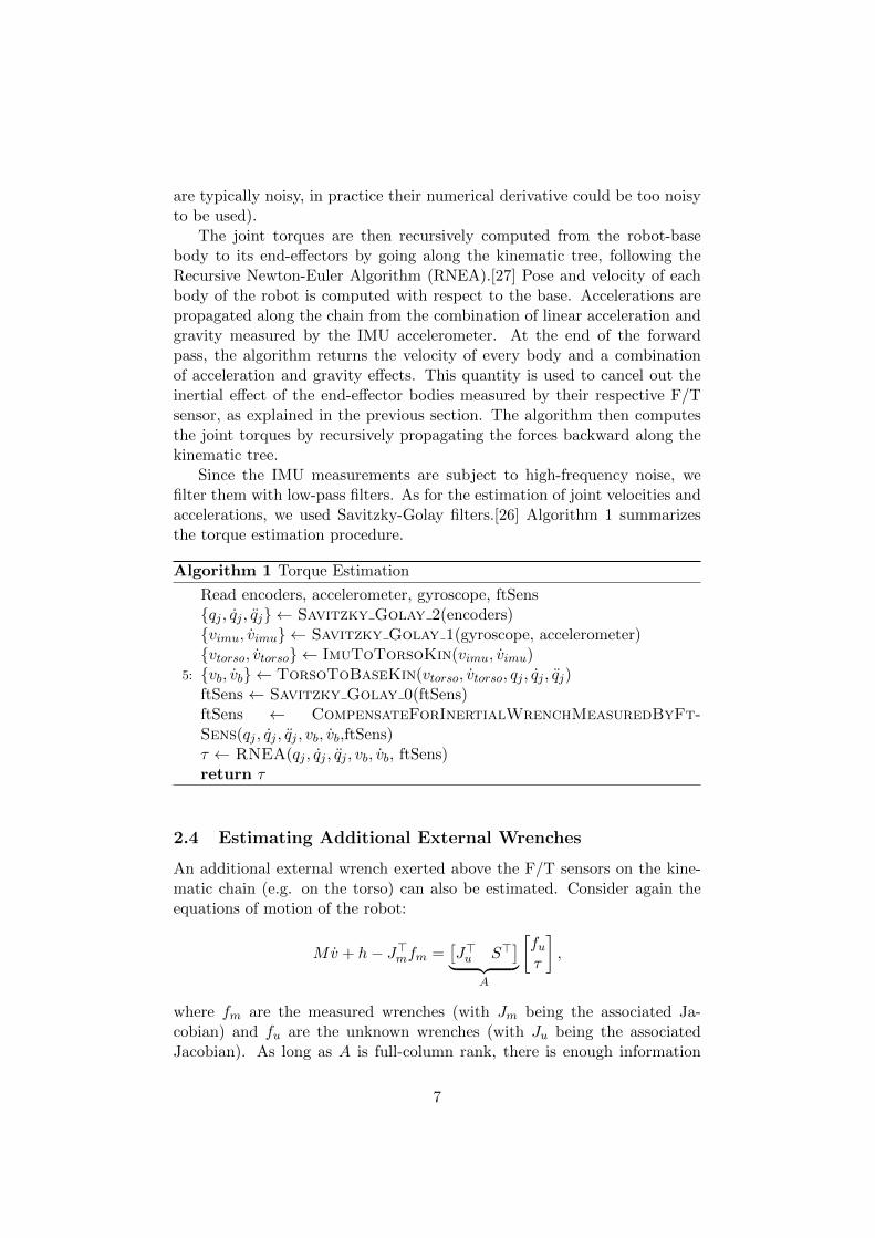
The joint torques are then recursively computed from the robot-basebody to its end-effectors by going along the kinematic tree, following theRecursive Newton-Euler Algorithm (RNEA).[27] Pose and velocity of eachbody of the robot is computed with respect to the base. Accelerations arepropagated along the chain from the combination of linear acceleration andgravity measured by the IMU accelerometer. At the end of the forwardpass, the algorithm returns the velocity of every body and a combinationof acceleration and gravity effects. This quantity is used to cancel out theinertial effect of the end-effector bodies measured by their respective F/Tsensor, as explained in the previous section. The algorithm then computesthe joint torques by recursively propagating the forces backward along thekinematic tree.

Since the IMU measurements are subject to high-frequency noise, wefilter them with low-pass filters. As for the estimation of joint velocities andaccelerations, we used Savitzky-Golay filters.[26] Algorithm 1 summarizesthe torque estimation procedure.

Algorithm 1 Torque Estimation

Read encoders, accelerometer, gyroscope, ftSens{qj , qj , qj} ← Savitzky Golay 2(encoders){vimu, vimu} ← Savitzky Golay 1(gyroscope, accelerometer){vtorso, vtorso} ← ImuToTorsoKin(vimu, vimu)

5: {vb, vb} ← TorsoToBaseKin(vtorso, vtorso, qj , qj , qj)ftSens ← Savitzky Golay 0(ftSens)ftSens ← CompensateForInertialWrenchMeasuredByFt-Sens(qj , qj , qj , vb, vb,ftSens)τ ← RNEA(qj , qj , qj , vb, vb, ftSens)return τ

2.4 Estimating Additional External Wrenches

An additional external wrench exerted above the F/T sensors on the kine-matic chain (e.g. on the torso) can also be estimated. Consider again theequations of motion of the robot:

Mv + h− J>mfm =[J>u S>

]︸ ︷︷ ︸A

[fuτ

],

where fm are the measured wrenches (with Jm being the associated Ja-cobian) and fu are the unknown wrenches (with Ju being the associatedJacobian). As long as A is full-column rank, there is enough information

7

to estimate τ using a least-squares procedure. In practice this means thatwe can only estimate one additional external wrench, namely rank(Ju) ≤ 6.Altogether five external wrenches can be applied on the robot: one for eachend-effector plus one on the kinematic tree delimitated by the four F/Tsensors. In most classical humanoid scenarios such as walking, push recov-ery and manipulation this assumption is verified. Complex scenarios withmultiple contacts on the robot’s body (e.g. both knees on the ground, bothelbows in contact) could not be properly handled by our method. Addingmore F/T sensors inside the robot’s limbs (similarly to the iCub robot)would increase the number of contact scenarios handled by the method.[14]

The critical point is to know on which link the additional external wrenchis applied, because this affects on which joints that wrench is creating torque.This problem can be solved by using tactile sensors[28], but at the momentHRP-2 does not have any. Alternatively, momenta/residual methods couldbe used [29, 8], but it is not clear whether they could work without knowingthe motor current. We decided to always assume to have an external wrenchon the torso, so that the robot can properly estimate the joint torques incase it is pushed on the torso. In case of no external wrench, the estimatedwrench should be close to zero. Alternatively, we can assume no externalwrench at all, in which case it is possible to use the n+6 equations of motionto estimate the n torque variables as:

τ = argminτ||M ˆv + h− J>mfm − S>τ ||2 = S(M ˆv + h− J>mfm) (2)

where . represents the estimated values. This is equivalent to assuming thatthe unknown wrench is applied to the floating base (i.e. Ju is a matrix thatselects only the base-link coordinates).

In any case, the torque estimation can be computed using a modifiedRNEA:[14] the measured wrenches have to be propagated from the four end-effectors back to the unknown-wrench link. This will automatically resultin the estimation of the joint torques, without any need to directly estimatethe unknown wrench. However, it is useful to monitor the unknown wrenchto check that, in case of no external contact, it remains small in magnitude.The unknown wrench fu can be computed as the wrench that makes thenet wrench on the associated link be equal to the time derivative of itsmomentum: ∑

i

fi + fu = Ivl + Ivl,

where I represents the spatial inertia of the link, vl is its spatial velocityand fi are the wrenches applied on the link by all the connected links.

8

3 Motor Identification

The previous section briefly recalled how joint torques are estimated fromthe classical sensors of a humanoid robot without direct joint-torque mea-surements; this estimation will be used to identify a model of the actuationof the robot. This section starts by describing and discussing the selectedactuation model, which is kept simple to allow a robust identification pro-cedure. Then, the identification is formulated as an optimization problem,which is solved by numerical methods. We finally briefly discuss practicalissues related to the data collection to ensure a good identification.

3.1 Linear Model

3.1.1 Generic rigid model

Considering DC motors as actuators and assuming a rigid transmission (i.e.no elasticity in the gear box), the joint torques τ are given by the differencebetween the motor torques τm and the friction torques τF :

τ = K1i︸︷︷︸τm

− (K2qj +K3sign(qj))︸ ︷︷ ︸τF

, (3)

where K1 ∈ Rn×n contains the motor drive gains, i ∈ Rn are the motor cur-rents, K2 ∈ Rn×n contains the viscous-friction coefficients, and K3 ∈ Rn×ncontains the Coulomb-friction coefficients. The same model also applies ifwe can control the motor voltage V , rather than the current i. Neglectingthe electrical dynamics, which is a reasonable assumption provided that thedynamics of the current amplifiers have much higher bandwidth than themotors, we have:

i =1

RV +

kbRqj︸︷︷︸ib

, (4)

where ib is proportional to the back electromotive torque, R is the motor coilresistance, and kb is a constant comprising the effect of the flux generatedby the coil. If we substitute (4) in (3), the equation maintains the same formbecause the back electromotive torque can be included inside the viscous-friction torque, being both terms proportional to qj . For this reason, inthe following we do not make any distinction between voltage and currentcontrol.

Overall our motor model is based on two simplifying assumptions: i) theelectrical dynamics is negligible, and ii) the transmission is perfectly rigid.While the first assumption is common in the literature [15, 19], the secondone constitutes one of the specific features of this work. Our experimentsshow that even using this simplified model we get significant improvementsover classic position control.

9

3.1.2 Model for HRP-2

HRP-2 is a high-quality industry-built robot which comes with the drawbackthat the low-level control implementation is closed source and thus preventsthe direct command of the current/voltage of the motors. However, we canspecify the desired joint angles qdj ∈ Rn, which are then used by the low-levelposition controller to compute the desired motor currents using a simpleproportional-derivative (PD) control law (with marginal modifications, aswe will see later):

i = K4 (qdj − qj)︸ ︷︷ ︸∆q

−K5qj . (5)

Substituting (5) in (3) and solving for ∆q, we get the following relationshipbetween the position tracking error ∆q and the joint torques τ :

∆q = K−14

(K−1

1 τ + (K−11 K2 +K5)qj +K−1

1 K3 sign(qj)),

which we can rewrite as:

∆q = Kττ +Kv qj +Kcsign(qj). (6)

This implies that having the motor current as control input is actually equiv-alent to having the desired joint angles as control input: in both cases thereis a linear relationship between the τ , qj , sign(qj) and the control input.

3.1.3 Linear identification

Having a linear model makes the identification straightforward because wecan use a least-squares fitting. Setting x> =

[Kτ Kv Kc

]as the deci-

sion variable, and assuming m collected samples, we can solve the followingoptimization problem for each motor:

minx∈R3

||Ax− b||2 (7)

where

A =

τ1 qj1 sign(qj1)...

......

τm qjm sign(qjm)

and b =

∆q1...

∆qm

.The optimal estimate is obtained by solving this quadratic problem (e.g.computing the pseudo-inverse of A, whose implementation is available inmost mathematic programming frameworks).

During the experiments on the robot, we observed that the Coulomb-friction term was not significantly improving the fitting. We therefore ne-glected it in practice. For the sake of clarity, we removed this term from themodel in the remaining of the paper.

10

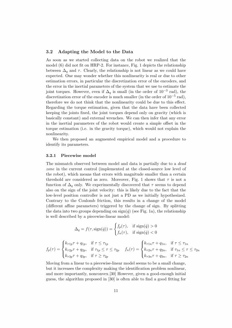
3.2 Adapting the Model to the Data

As soon as we started collecting data on the robot we realized that themodel (6) did not fit on HRP-2. For instance, Fig. 1 depicts the relationshipbetween ∆q and τ . Clearly, the relationship is not linear as we could haveexpected. One may wonder whether this nonlinearity is real or due to otherestimation errors, in particular the discretization error of the encoders, andthe error in the inertial parameters of the system that we use to estimate thejoint torques. However, even if ∆q is small (in the order of 10−3 rad), thediscretization error of the encoder is much smaller (in the order of 10−5 rad),therefore we do not think that the nonlinearity could be due to this effect.Regarding the torque estimation, given that the data have been collectedkeeping the joints fixed, the joint torques depend only on gravity (which isbasically constant) and external wrenches. We can then infer that any errorin the inertial parameters of the robot would create a simple offset in thetorque estimation (i.e. in the gravity torque), which would not explain thenonlinearity.

We then proposed an augmented empirical model and a procedure toidentify its parameters.

3.2.1 Piecewise model

The mismatch observed between model and data is partially due to a deadzone in the current control (implemented at the closed-source low level ofthe robot), which means that errors with magnitude smaller than a certainthreshold are considered as zero. Moreover, Fig. 1 shows that τ is not afunction of ∆q only. We experimentally discovered that τ seems to dependalso on the sign of the joint velocity: this is likely due to the fact that thelow-level position controller is not just a PD as we initially hypothesized.Contrary to the Coulomb friction, this results in a change of the model(different affine parameters) triggered by the change of sign. By splittingthe data into two groups depending on sign(q) (see Fig. 1a), the relationshipis well described by a piecewise-linear model:

∆q = f(τ, sign(q)) =

{fp(τ), if sign(q) > 0

fn(τ), if sign(q) < 0

fp(τ) =

kτ1pτ + q1p, if τ ≤ τ1p

kτ2pτ + q2p, if τ1p ≤ τ ≤ τ2p

kτ3pτ + q3p, if τ ≥ τ2p

fn(τ) =

kτ1nτ + q1n, if τ ≤ τ1n

kτ2nτ + q2n, if τ1n ≤ τ ≤ τ2n

kτ3nτ + q3n, if τ ≥ τ2n

Moving from a linear to a piecewise-linear model seems to be a small change,but it increases the complexity making the identification problem nonlinear,and more importantly, nonconvex.[30] However, given a good-enough initialguess, the algorithm proposed in [30] is often able to find a good fitting for

11

40 20 0 20 40 60 80τ [Nm]

0.0040.0030.0020.0010.0000.0010.0020.0030.004

∆q [r

ad]

Positive velocityNegative velocity

(a) Data separated depending on thesign of the joint velocity.

40 20 0 20 40 60 80τ [Nm]

0.0040.0030.0020.0010.0000.0010.0020.0030.0040.005

∆q [r

ad]

DataModel

(b) The linear model identified with asymmetric penalty function (i.e. least-squares).

150 100 50 0 50 100τ [Nm]

0.0250.0200.0150.0100.0050.0000.0050.0100.015

∆q [r

ad]

DataModel

(c) The two piecewise-linear models (forpositive and negative velocities).

40 20 0 20 40 60 80τ [Nm]

0.0040.0030.0020.0010.0000.0010.0020.0030.004

∆q [r

ad]

DataModel

(d) The linear model identified with anasymmetric penalty function.

Figure 1: Torque τ vs. position error ∆q for the right knee (a, b, d) andright hip-pitch (c) joints of HRP-2. These data have been collected on oneposition-controlled joint keeping qdj constant and applying external forces.The joint is nearly static, so that qj ≈ 0. From (6), we expect ∆q = Kττ ,but the data clearly do not fit.

12

the data. This algorithm only works for convex piecewise-linear functions,whereas our function is nonconvex.2 For this reason, we slightly modifiedthe algorithm so that it could work for our special nonconvex case.

3.2.2 Piecewise-Linear Fitting

The algorithm is rather simple. We start with an initial guess on the twoswitching points τ1, τ2 between the three linear models (we will hereafterdrop the p and n sub-indices for notation simplicity; therefore, τ1 representseither τ1p or τ1n, and so forth). Then, we repeat the following procedureuntil convergence or until we reach the maximum number of iterations:

• update kτ1, kτ2, kτ3, q1, q2, q3 by separately fitting the three linear mod-els to the three datasets

• update τ1 to the intersection point between line 1 and line 2

• update τ2 to the intersection point between line 2 and line 3

The algorithm converges when τ1 and τ2 do not change between two succes-sive iterations. Remarkably, the resulting model is continuous by construc-tion. We empirically noticed that the algorithm works better if we boundthe slope of the central line (k2), which is reasonable because we know, fromobserving the data, that it always has a large positive slope.

For identifying f(.) on the leg joints, we set the initial guess to τ1 = −0.5and τ2 = 0.5, and we set the maximum number of iterations to 10. Fig. 1cshows the result for the right hip-pitch joint. Most of the time, the algorithmconverged before reaching the maximum number of iterations. Even if notperfect, the results seem satisfactory for the scope of the application.

3.2.3 Limits of the Model

Despite the good fitting of the model to the data, this approach proved un-successful for a number of reasons, so we decided to pursue another strategy(see next subsection). The main reason that led us to this decision was thatthe resulting torque control was unstable in open-loop (i.e. with zero feed-back gains). We believe that this was mainly due to the fact that the twomodels are not exactly separated by the sign of the joint velocity. In par-ticular, the switch between the two models (i.e. when the velocity changessign) is critical and it is hard to identify. Having access to the code of thelow-level control of HRP-2 would drastically simplify the understanding ofthis effect and of how we could compensate for it, but for now this is notthe case. Since our piecewise-linear model did not perfectly fit the data, in

2A piecewise-linear function is convex if and only if it can be expressed as the maximumover a set of linear function (see [31], Example 3.5). This is not the case for our model.

13

some regions it was over-estimating the value of ∆q necessary to generate acertain τ , triggering instability.

As secondary reasons, the extended model made both the identificationand the control more complex. The piecewise-linear fitting algorithm doesnot always converge to a good solution, so it requires the user to provide aninitial guess that may be different for each joint. The controller with theextended model also requires an estimation of the sign of the acceleration,which needs to be approximated with a smooth function to avoid discon-tinuities in the control input. This introduces an additional parameter totune the smoothing of the sign function.

3.3 Asymmetric-Penalty Identification

Given the failure of the approach described in the previous subsection, wedecided to go back to the original linear model. To account for the factthat the model could not exactly fit the data, we modified the identificationproblem. Rather than trying to find the best fit in the least-squares sense,we now look for the best fit that almost never over-estimates ∆q in absolutevalue. This conservative approach guarantees that the torque controller willbe stable in open-loop. In other words, we penalize more over-estimatingthan under-estimating. The result of this asymmetric penalty function canbe seen in Fig. 1d: the blue line is almost never higher than the red dots inabsolute value.

To formulate the new identification problem, the data {A, b} are sepa-rated into two sets {Apos, bpos} and {Aneg, bneg} depending on the sign of∆q, where each set has mpos and mneg pair elements, respectively. Theoptimization problem is then formulated as:

minx∈R3

mpos∑i=1

Φ(aposi x− bposi ) +mneg∑i=1

Φ(−anegi x+ bnegi ) (8)

with

Φ(z) =

{wz2, if z > 0

z2, otherwise

where aposi /anegi is the i-th row of Apos/Aneg, bposi /bnegi is the i-th elementof bpos/bneg, and w > 1 is a user-defined parameter that weighs how muchover-estimation is penalized more with respect to under-estimation.

This problem is convex, so we can solve it with, for instance, Newton’smethod. Alternatively, we can reformulate it as a Quadratic Program (QP).To this end, we introduce two auxiliary variables yp, yn and we reformulate

14

(8) as:min

x∈R3,yp∈Rm,yn∈Rmw||yp||2 + ||yn||2

s. t. yp ≥ Ax− byn ≥ −Ax+ b

yp, yn ≥ 0,

(9)

where:

A =

[Apos

−Aneg]

b =

[bpos

−bneg]

At the optimum, the elements of yp corresponding to under-estimation (i.e.Ax < b) are zero, while those corresponding to over-estimation are exactlyequal to Ax − b (which is then penalized with the weight w in the costfunction). Similarly, at the optimum the elements of yn corresponding toover-estimation are zero, while those corresponding to under-estimation areequal to−Ax+b (which is penalized without any weight in the cost function).In other words, the optimum values of yp and yn are complementary, thatis yp>yn = 0. The advantage of this new formulation is that we can solveit with any QP solver. The disadvantage is that we have introduced 2mnew variables and 2m inequality constraints, which could make the problemintractable if m — the number of data samples — is too large (e.g. bothCVX [32] and qpOases[33] failed for m > 104). In practice we saw that103 samples (obtained by downsampling the original data taken at 1 kHz)are enough to identify the model, which can then be validated on a largernumber of samples.

3.3.1 Two-Stage Identification

We noticed that, especially for some joints, it was beneficial to split the iden-tification problem into two parts. First, only use the zero-velocity (i.e. belowsome threshold) samples to identify kτ ; then, only use the nonzero-velocitysamples, together with the previously identified value of kτ , to identify kv.In some cases, this procedure improves the identification of kτ . The reasonis that kv is always 1 or 2 orders of magnitude greater than kτ , so when thejoint velocity is not zero most of ∆q is due to friction, making the identifi-cation of kτ poorly conditioned.

3.4 Data Collection

The collection of the data used for identification is crucial to the final re-sult. The fact that the linear model cannot fit the data well (e.g. becauseof the deadzone) implies that the identification will not easily generalizeoutside of the observed range. It is then important to make sure that thecollected data properly cover the whole operative region of τ and q. A di-rect consequence is that we cannot identify the model using only low or

15

medium velocities/torques and expect the model to work well for large ve-locities/torques. To get both large velocities and large torques, we split thedata collection into two parts. The first part samples large torques and zerovelocities, so that we can identify kτ in (6). In the second part we use largevelocities, so that we can identify kv.

3.4.1 High-torque data collection

In this phase we position the robot in a predefined set of configurationsusing the standard high-gain position control of HRP-2. The user can thenapply torque on all the joints by exerting forces on the robot end-effectors.The aim is to create as large as possible torques. For the identification ofthe leg joints we can lift the robot and apply forces on its feet. Differentconfigurations are necessary to generate large torques on all the joints.

3.4.2 High-velocity data collection

The identification of frictions can be automatized because we do not needthe user to apply external forces. We commanded to the position controlleran increasing-amplitude sinusoid:

qdj (t) = (a0 + at) sin(2πft)

where a0 is the initial amplitude, a regulates the speed of increase of thesinusoid amplitude, and f is the sinusoid frequency.

3.4.3 Noncausal Estimation

Since the identification is based on the estimation of the joint velocitiesand accelerations, we can expect to get better results by using noncausalestimations. This means that at time t we do not estimate qj(t), but werather estimate qj(t−td), where td is the estimation delay. The same appliesfor q, v and the force/torque measurements.

4 Control

The control is made up of two terms that we describe in the first subsection:a feedforward term to compensate for the dynamics of the actuator, and afeedback term to reject noise and unmodeled dynamics. We then presentan inverse dynamics scheme, which we used in the experiments to generatethe reference joint torques. In the second subsection, we reformulate thecontrol law in order to ease its experimental comparison with the positioncontroller.

16

4.1 Control law

4.1.1 Feedforward

The feedforward comes from the identification of the model equation (6),carried out in the previous section. The feedforward control law is:

∆q = Kττ∗ +Kv qj , (10)

where τ∗ are the commanded joint torques.

4.1.2 Torque feedback

The feedback consists in a proportional-integral control law:

τ∗ = τd +Kpeτ +Ki

∫eτdt (11)

where eτ = (τd − τ) ∈ Rn is the torque tracking error, Kp,Ki ∈ Rn×n arerespectively the proportional and integral gain matrices (diagonal positive-definite), τd ∈ Rn are the desired joint torques and τ ∈ Rn are the estimatedjoint torques (2).

In practice, we did not observe any improvement of the control behav-ior when modifying the integral term. Since the position control does notcomprehend an integral term, we decided not to include it and considerKi = 0 in the remaining of the paper. We could possibly add a disturbanceobserver, which has been already used for joint-torque control.[19]

4.1.3 Inverse dynamics

In the experiments, the desired joint torques are computed from an inverse-dynamics control law[34] tracking a reference trajectory of the actuateddegrees of freedom.3 Given a desired joint trajectory {qj(t)d, qj(t)d, qj(t)d}and a desired contact force fd, the desired joint torques are:

τd = Mj qdj + hj − J>j f∗ +Kseq +Kdeq (12)

withf∗ = fd +Kfef

where Mj ∈ Rn×n is the joint-space mass matrix (i.e. the bottom-right

corner of M), hj ∈ Rn are the last n elements of h, Jj is the part of theJacobian corresponding to the actuated joints, eq = qdj − qj is the position

3When discussing estimation in Section 2 we considered a floating-base model of therobot. However, for the sake of simplicity, the controller rather considers a fixed-basemodel. This is justified by the fact that, being the robot attached to a lift device, themotion of its base was limited. In the future we plan to switch to a floating-base inverse-dynamics controller such as the one presented in [6].

17

tracking error, ef = fd − f is the force tracking error, and Ks ∈ Rn×n,Kd ∈ Rn×n, Kf ∈ Rk×k are the stiffness, damping and force gain matrices(diagonal positive-definite), respectively.

4.2 Gain Comparison

The control law can be parametrized by the user-defined gains (Kp, Ks,Kd, Kf ) and by the gains identified from the motor characteristics (Kτ ,Kv). Substituting (11) in (10), using (12) and the estimates ˆqj = qj and

τ = Mjˆqj + hj − J>j f , the control law can be finally separated in two main

parts, corresponding to the feedforward and feedback components, as:

∆q =Kτ (Mj qdj + hj − J>j fd) +Kv

ˆqj (13)

+K6eq +K7eq +K8eq +K9ef (14)

where:

K6 = Kτ (I +Kp)Ks

K7 = Kτ (I +Kp)Kd

K8 = KτKpMj

K9 = −Kτ (KpJ>j (I +Kf ) + J>j Kf ).

The terms in (13) correspond to the feedforward action. More precisely,the first term decouples the articulated dynamics, while the second termcompensates for the friction. The terms in (14) correspond to the feedbackaction on the position, velocity, acceleration and force. The feedforwardpart (13) is independent of the position and force tracking errors.

Since Kτ is given by the motor identification (it is not defined by theuser), selecting one of the two sets of gains {K6,K7,K8,K9} or {Kp,Ks,Kd,Kf}implies an immediate correspondence in the other set.

There is a direct correspondence with the position-based PD controlleroriginally implemented on the robot. The errors in position eq appears inboth controllers, while the other errors eq, eq and ef as well as the feedfor-ward are only considered in our proposed torque control. It is now possibleto compare the tuning of both controllers. When the diagonal componentsof K6 are greater than one, it implies that the torque controller is using feed-back gains larger than those used by the native low-level position controllerof HRP-2. Conversely, diagonal components of K6 lower than one implya smaller position feedback for the torque controller than for the positioncontroller.

18

(a) Force tracking experi-ment.

(b) Motion tracking ex-periment.

Figure 2: Experimental setup.

5 Experimental Results

5.1 Experimental Setup

We carried out all the experiments on the 6 joints of the right leg of HRP-2.In the motion-control experiment HRP-2 was hanging in the air, attached toa lift device by means of two strings tied to its shoulders (see Fig. 2b). In theforce-control experiment it was instead standing on both feet (see Fig. 2a),while the strings prevented the robot from falling. As far as the estimationis concerned, we used a window of 80 samples. Since the sampling time was1 ms, this resulted in an estimation delay of 40 ms (i.e. half the windowsize). We tested the controller also with smaller/larger window sizes, but 80seemed to be the best trade-off between stability and performance. We usedfirst-order polynomials to filter the F/T sensor and the IMU measurements,and second-order polynomials for the encoders. We set the torque-feedbackgains Kp to 2 for all the 6 joints.

The tuning of the estimation and control parameters (i.e. window lengthand feedback gains) has been empirically performed. To keep things simple,we decided to use the same gain for all the joints and the same delay (andcut-off frequency) for all the sensors. However, we believe that there is roomfor improvement in this direction. We saw that by increasing the estimationwindow we got smoother feedback signals, which allowed us to use highergains, so improving the performance of the controller. On the other side,increasing the estimation window also increases the estimation delay, which

19

Table 1: Identified motor parameters.

Joint 103kτ 103kvHip yaw 0.212 13.0Hip roll 0.030 6.332Hip pitch 0.12 7.0Knee 0.051 6.561Ankle pitch 0.177 7.698Ankle roll 0.240 6.0

at a certain point outweighs the improvement coming from using highergains. Finding the best trade-off between estimation smoothing/delay andfeedback gains is still an open problem, which might be an interesting subjectfor future work.

5.2 Motor Identification

We collected the data following the procedure described in Section 3.4 and wethen used them to identify the motor parameters, as described in Section 3.3.We set the weight of the asymmetric penalty function (8) to w = 100.Table 1 lists the identified parameters. Fig. 3 depicts how the model fitsthe data for the ankle-pitch joint. Using the symmetric penalty function,the model tends to over-estimate the data for large velocities. In practicethis resulted in an unstable controller (i.e. the joint accelerating as soonas a certain velocity was reached, even when lowering the feedback gains tozero). With the asymmetric penalty, the model no longer over-estimates thedata, while the quality of the fit for small velocity remains of similar quality.

5.3 Motion Control

Table 2: Average squared tracking error (in rad 103) for the stairs-climbing

trajectory: N−1√∑N

i=1(qd(ti)− q(ti))2, where N is the number of samples.

Joint Pos.ctrl.

TorquectrlK6 = 1

TorquectrlK6 = 0.5

TorquectrlK6 = 0.25

TorquectrlK6 = 0.1

Hip roll 0.020 0.005 0.008 0.016 0.040Hip pitch 0.056 0.018 0.035 0.064 0.139Knee 0.115 0.060 0.061 0.067 0.094Ankle pitch 0.064 0.017 0.034 0.063 0.148Ankle roll 0.029 0.015 0.029 0.059 0.136

20

2.0 1.5 1.0 0.5 0.0 0.5 1.0 1.5 2.0qj [rad/s]

0.0200.0150.0100.0050.0000.0050.0100.0150.020

∆q−Kττ

[rad

] DataModel

(a) Symmetric penalty fitting.

0.004 0.002 0.000 0.002Residual [rad]

0

5000

10000

15000

Num

ber o

f sam

ples

(b) Symmetric penalty residuals.

2.0 1.5 1.0 0.5 0.0 0.5 1.0 1.5 2.0qj [rad/s]

0.0150.0100.0050.0000.0050.0100.0150.020

∆q−Kττ

[rad

] DataModel

(c) Asymmetric penalty fitting.

0.004 0.002 0.000 0.002Residual [rad]

0

5000

10000

15000

Num

ber o

f sam

ples

(d) Asymmetric penalty residuals.

Figure 3: Friction identification for the ankle-pitch joint: comparison of thetwo penalty functions: [top] symmetric penalty (7) [bottom] asymmetricpenalty (8). The two plots on the left display the friction part of the model(∆q −Kττ) with respect to the velocity (qj). The data have been collectedtracking a sinusoidal reference with increasing amplitude. The two plotson the right display the distribution of the residuals (|Kττ +Kv qj | − |∆q|):the symmetric penalty tends to overestimate the friction for high velocities(indeed we have positive residuals), while the asymmetric penalty mostlyunderestimates while keeping a fit of similar quality.

Table 3: Maximum tracking error (in rad 103) for the stairs-climbing tra-jectory.

Joint Pos.ctrl.

TorquectrlK6 = 1

TorquectrlK6 = 0.5

TorquectrlK6 = 0.25

TorquectrlK6 = 0.1

Hip roll 4.79 2.35 2.95 2.85 5.76Hip pitch 17.01 7.87 7.83 10.40 22.78Knee 61.86 39.64 41.55 41.19 49.33Ankle pitch 19.56 4.84 5.92 10.39 22.43Ankle roll 6.11 2.55 3.69 6.80 16.44

21

0 1 2 3 4 5 6 7 8 9Time [s]

0.250.200.150.100.050.000.050.100.150.20

q j [r

ad]

qj

q dj

(a) Hip-roll position tracking

0 1 2 3 4 5 6 7 8 9Time [s]

1.2

1.0

0.8

0.6

0.4

q j [r

ad]

qj

q dj

(b) Ankle position tracking

0 1 2 3 4 5 6 7 8 9Time [s]

201510

505

101520

q j−qd j

[103

rad]

(c) Hip-roll error, position control

0 1 2 3 4 5 6 7 8 9Time [s]

201510

505

101520

q j−qd j

[103

rad]

(d) Ankle error, position control

0 1 2 3 4 5 6 7 8 9Time [s]

201510

505

101520

q j−qd j

[103

rad]

(e) Hip-roll error, torque control K6 = 1

0 1 2 3 4 5 6 7 8 9Time [s]

201510

505

101520

q j−qd j

[103

rad]

(f) Ankle error, torque control K6 = 1

0 1 2 3 4 5 6 7 8 9Time [s]

201510

505

101520

q j−qd j

[103

rad]

(g) Hip-roll error, torque control K6 =0.25

0 1 2 3 4 5 6 7 8 9Time [s]

201510

505

101520

q j−qd j

[103

rad]

(h) Ankle error, torque control K6 =0.25

Figure 4: Comparison of the motion tracking accuracy for the position con-troller and for the torque controller. The results from two joints are displayed(hip roll and ankle pitch). Three different controllers are exhibited: originallow-level position controller, inverse dynamics with the same gains than theposition controller (K6 = 1) and inverse dynamics with 25% feedback gains(K6 = 0.25). At large scale, the position trajectories are similar for thethree controllers (the top row shows the results for the position controller,but the other two controllers would look just the same). Compared to theposition controller, the torque controller with similar gain (K6 = 1) is muchmore accurate (lower tracking error). The torque controller with lower gain(K6 = 0.25) has a comparable accuracy.22

We compared the capabilities of tracking a joint-space trajectory of ournew controller with those of the standard low-level position controller ofHRP-2. The trajectory is the swinging motion of the right leg computedto make the robot climb some stairs. This motion is very demanding withrespect to the capabilities of the motors, by asking a large displacement (ofthe swing leg) in a short time. We experimentally know that this movementis close to the dynamic limits of the robot.

We tested the position controller against four different gain tuning ofinverse-dynamics controller, corresponding to 100%, 50%, 25% and 10% ofthe standard position-control gains (i.e. K6 was equal to 1, 0.5, 0.25 and0.1, respectively). Table 2 and 3 respectively report the average and maxi-mum tracking error for the each joint and each controller. Fig. 4 shows thetracking error trajectory for two joints (hip roll and ankle pitch) and threecontrollers, to visualize the different shapes of the errors. With K6 = 1the inverse-dynamics controller performs significantly better than the posi-tion controller, obtaining lower maximum and average tracking errors on alljoints. With K6 = 0.5 the inverse-dynamics controller still performs betterthan the position controller on all joints (except the average error of theankle roll, which is equivalent). With K6 = 0.25 the average errors on mostjoints are almost equivalent (except ankle roll/knee, which are significantlyworse/better), but the inverse-dynamics controller still results in lower max-imum errors (except for the ankle roll). Finally, with K6 = 0.1 the positioncontroller performs better than the inverse-dynamics controller on all jointsbut the knee.

5.4 Force Control

This experiment tests the capabilities of the torque controller to track areference Cartesian force. The right foot of HRP-2 is positioned in con-tact with a rigid fixed object (a small pile of bricks, see Fig. 2). We thencommanded to the inverse-dynamics controller a sinusoidal force referenceon the z axis (vertical direction), while maintaining the force on the otheraxes to zero. The position gains were set to 10% of the standard position-control gains (i.e. K6 = 0.1), which corresponds to the lowest gain withmotion-tracking accuracy similar to the position controller, obtained fromthe previous experiment. The reference joint angles were set to be compati-ble with the force task. By keeping significant position-feedback gains, someslight motion occurring during the experiment would likely cause interfer-ences between the joint-position and the force tracking. However, it doesnot seem relevant to set these gains to zero, mainly for security reasons (incase the robot lost the contact the position feedback would have preventedit from moving too far away from the initial configuration). We empiricallyset all the force feedback gains Kf to 1, which is the higher values beforeobserving instability in the control. Fig. 5 shows the results. The robot is

23

0 5 10 15 20 25Time [s]

200

20406080

100120

Forc

e [N

]ForceDesired force

(a) Force tracking on the x axis.

0 5 10 15 20 25Time [s]

200

20406080

100120

Forc

e [N

]

ForceDesired force

(b) Force tracking on the y axis.

0 5 10 15 20 25Time [s]

200

20406080

100120

Forc

e [N

]

ForceDesired force

(c) Force tracking on the z axis.

Figure 5: Tracking of a sinusoidal force reference on the z axis of the rightfoot while keeping other force directions to zero. An overshoot of maximum10% is observed at the sinusoid apex. The same 10% are observed as acoupling on the X axis. No significant delay affects the tracking.

able to track the desired force sinusoid; the ≈ 10% overshoot is likely dueto the above-mentioned conflict between force and position tracking.

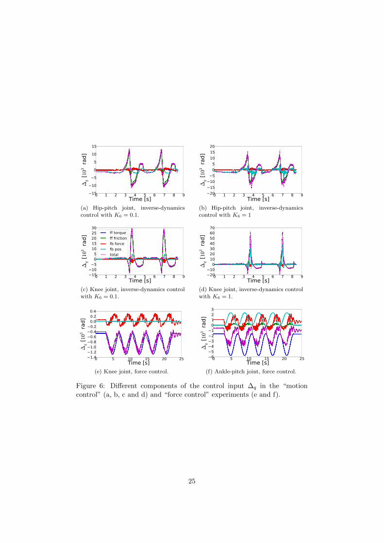
5.5 Analysis of Different Control Components

The final torque control is a complex mix of feedforward and feedback terms.This section analyses the different components of the control input ∆q in thetwo previous experiments (i.e. motion control and force control) to providesome intuitions regarding the effect of each component on the quality of thepresented results. Our goal is to understand to what extent each compo-nent is contributing to the final control input. Recall from Section 4.2 thatwe can decompose the control input in six different parts, two feedforwardcomponents and four feedback components:

∆q = Kτ (Mj qdj + h− J>fd)︸ ︷︷ ︸

feedforward torque

+ Kvˆqj︸ ︷︷ ︸

feedforward friction

+ K6eq︸ ︷︷ ︸feedback position

+ K7eq︸ ︷︷ ︸feedback velocity

+ K8eq︸ ︷︷ ︸feedback acceleration

+ K9ef︸ ︷︷ ︸feedback force

We reproduced the two previous experiments and measured the importanceof each of these six terms in the control. Fig. 6 shows the values of the two

24

0 1 2 3 4 5 6 7 8 9Time [s]

15

10

5

0

5

10

15

∆q [1

03 ra

d]

(a) Hip-pitch joint, inverse-dynamicscontrol with K6 = 0.1.

0 1 2 3 4 5 6 7 8 9Time [s]

201510

505

101520

∆q [1

03 ra

d](b) Hip-pitch joint, inverse-dynamicscontrol with K6 = 1

0 1 2 3 4 5 6 7 8 9Time [s]

1510

505

1015202530

∆q [1

03 ra

d]

ff torqueff frictionfb forcefb postotal

(c) Knee joint, inverse-dynamics controlwith K6 = 0.1.

0 1 2 3 4 5 6 7 8 9Time [s]

20100

10203040506070

∆q [1

03 ra

d]

(d) Knee joint, inverse-dynamics controlwith K6 = 1.

0 5 10 15 20 25Time [s]

1.41.21.00.80.60.40.20.00.20.4

∆q [1

03

rad]

(e) Knee joint, force control.

0 5 10 15 20 25Time [s]

6543210123

∆q [1

03

rad]

(f) Ankle-pitch joint, force control.

Figure 6: Different components of the control input ∆q in the “motioncontrol” (a, b, c and d) and “force control” experiments (e and f).

25

feedforward components and the position and force feedback componentsfor two different joints during the motion-control experiment (with both themaximum and the minimum feedback gains) and force-control experiment.By looking at these data we can draw that:

• during motion control the “feedforward friction” is contributing themost, followed by the “feedback position”;

• during force control the “feedforward torque” is contributing the most,followed by the “feedback force” (and the “feedback position” for theankle-pitch joint).

This means that in motion control the proposed torque controller is approx-imately acting as a standard position controller plus a friction compensa-tion. On the contrary, in force control the “feedforward torque” componentis playing an important role in the control, which justifies the existence ofthat part in the control law. Most probably it is the term J>fd the onecontributing the most between the three terms composing the feedforwardtorque, given that inertial and bias torques are negligible in this scenario.

From Fig. 6f it can also be noticed that the “feedback position” signifi-cantly contributed to the force control for certain joints. This is due to thefact that the contact was not perfectly rigid, so some joints slightly movedduring the experiment affecting (likely negatively) the force tracking.

6 Conclusions and Future Work

This paper discussed the implementation of torque control on the humanoidrobot HRP-2. Contrary to most previous works on the subject — but like90% of nowadays robots — our platform does not have joint-torque sensorsand its software interface does not allow the user to directly control themotor currents/voltages. This makes the control of the joint torques morechallenging on this hardware than on robots that were built to be torquecontrolled. We list hereafter the main contributions of this work.

• Our experimental setup shows that it is possible to implement torquecontrol on a robot that was originally built to be position controlled,and we can use it to control its motion and its contact forces.

• We described the implementation on the physical robot of the completeframework, composed by estimation, identification and control.

• Torque control, together with inverse dynamics, has been experimen-tally proved to produce better motion tracking than position control(i.e. improved accuracy for similar gains, or reduced gains while pre-serving accuracy). While this was well-known for torque-sensor basedtorque control, it is a nontrivial result for the torque control proposedin this paper.

26

• Our analysis shows that in motion control the most important partof our control framework is the feedforward friction compensation,whereas in force control the most important part is the torque feed-forward component. The dominance of the feedforward terms in thecontrol action validates our choice to use a simplified actuator modeland our identification procedure.

• We proposed an asymmetric-penalty identification that tends to pre-serve the stability of the controller (e.g. by avoiding over-compensatingfriction), along with two numerical formulations (either as a convexoptimization problem, or as a QP).

While the presented results are very promising, there is still room forimprovement, especially in the identification and the estimation. Using anapproximated model for the relationship between the joint torques and theposition is interesting because it simplifies the identification and avoids in-stability. However, the simplified model is arbitrary (we selected the rele-vant terms from our subjective observations), and some unidentified termsare now missing to obtain a perfect fit. Another important point is thatthe identified model is currently only used by the controller. The stateestimation algorithm could also exploit it to predict the future state andso nullify estimation delays. We also plan to experiment with DisturbanceObservers, as they have already been used to improve the performances ofother torque-control architectures.[19]

To conclude, this work opens a new interesting direction for the controlof “position-controlled” robots (i.e. stiff robots without joint-torque sen-sors), which could benefit from the presented torque-control architecture toimprove their performances, both in motion-tracking and in force-trackingtasks.

Acknowledgements

This work was supported by Euroc (FP7 Grant Agreement 608849), En-tracte (ANR Grant Agreement 13-CORD-002-01) and Koroibot (ICT-2013-10 project number 611909).

References

[1] Francesco Nori, Silvio Traversaro, Jorhabib Eljaik, Francesco Romano,Andrea Del Prete, and Daniele Pucci. iCub Whole-Body Controlthrough Force Regulation on Rigid Non-Coplanar Contacts. Frontiersin Robotics and AI, 2, 2015.

[2] Oussama Khatib, Peter Thaulad, and Jaeheung Park. Torque-positiontransformer for task control of position controlled robots. 2008 IEEE

27

International Conference on Robotics and Automation, pages 1729–1734, May 2008.

[3] Jun Nakanishi, Michael Mistry, and Stefan Schaal. Inverse dynamicscontrol with floating base and constraints. In Robotics and Automation,2007 IEEE International Conference on, number April, pages 10–14,2007.

[4] Mrinal Kalakrishnan, Jonas Buchli, Peter Pastor, Michael Mistry, andStefan Schaal. Learning, planning, and control for quadruped locomo-tion over challenging terrain. The International Journal of RoboticsResearch, 30(2):236–258, November 2010.

[5] Layale Saab, Oscar E. Ramos, Nicolas Mansard, Philippe Soueres, andJean-yves Fourquet. Dynamic Whole-Body Motion Generation underRigid Contacts and other Unilateral Constraints. IEEE Transactionson Robotics, 29(2):346–362, 2013.

[6] Andrea Del Prete and Nicolas Mansard. Addressing Constraint Robust-ness to Torque Errors in Task-Space Inverse Dynamics. In Robotics,Science and Systems (RSS), Rome, 2015.

[7] Oscar E. Ramos, Nicolas Mansard, Olivier Stasse, Jean-bernard Hayet,and Philippe Soueres. Towards reactive vision-guided walking on roughterrain: an inverse-dynamics based approach. International Journal ofHumanoid Robotics, 2, 2014.

[8] Sami Haddadin, Alin Albu-Schaffer, Alessandro De Luca, and GerdHirzinger. Collision detection and reaction: A contribution to safe phys-ical Human-Robot Interaction. 2008 IEEE/RSJ International Confer-ence on Intelligent Robots and Systems, pages 3356–3363, September2008.

[9] Andrea Del Prete, Francesco Nori, Giorgio Metta, and Lorenzo Na-tale. Prioritized Motion-Force Control of Constrained Fully-ActuatedRobots: ”Task Space Inverse Dynamics”. Robotics and AutonomousSystems, 63:150–157, 2015.

[10] Oussama Khatib. A unified approach for motion and force control ofrobot manipulators: The operational space formulation. IEEE Journalon Robotics and Automation, 3(1):43–53, February 1987.

[11] R. Volpe and P. Khosla. A theoretical and experimental investigationof explicit force control strategies for manipulators. IEEE Transactionson Automatic Control, 38(11):1634–1650, 1993.

28

[12] Brian Stewart Randall Armstrong. Dynamics for Robot Control: Fric-tion Modeling and Ensuring Excitation During Parameter Identifica-tion. PhD thesis, Stanford University, 1988.

[13] Kenji Kaneko and Fumio Kanehiro. Design of prototype humanoidrobotics platform for HRP. In Intelligent Robots and Systems, 2002.IEEE/RSJ International Conference on., 2002.

[14] Matteo Fumagalli, Serena Ivaldi, Marco Randazzo, Lorenzo Natale,Giorgio Metta, Giulio Sandini, and Francesco Nori. Force feedback ex-ploiting tactile and proximal force/torque sensing. Autonomous Robots,33(4):381–398, April 2012.

[15] Christian Ott, Alin Albu-Schaffer, and Gerd Hirzinger. Comparison ofadaptive and nonadaptive tracking control laws for a flexible joint ma-nipulator. In Intelligent Robots and Systems (IROS), 2002 IEEE/RSJInternational Conference on, 2002.

[16] Thiago Boaventura, Michele Focchi, Marco Frigerio, Jonas Buchli,Claudio Semini, Gustavo A. Medrano-Cerda, and Darwin G. Caldwell.On the role of load motion compensation in high-performance forcecontrol. In Intelligent Robots and Systems, IEEE/RSJ InternationalConference on, pages 4066–4071. Ieee, October 2012.

[17] Mehrdad R. Kermani, Rajnikant V. Patel, and Mehrdad Moallem. Fric-tion identification and compensation in robotic manipulators. IEEETransactions on Instrumentation and Measurement, 56(6):2346–2353,2007.

[18] Luc Le Tien and Alin Albu-Schaffer. Friction Observer and Compen-sation for Control of Robots with Joint Torque Measurement. In 2008IEEE/RSJ International Conference on Intelligent Robots and Systems,pages 22–26, 2008.

[19] Nicholas Paine, Sehoon Oh, and Luis Sentis. Design and Con-trol Considerations for High-Performance Series Elastic Actuators.IEEE/ASME Transactions on Mechatronics, 19(3):1080–1091, 2014.

[20] Kyoungchul Kong, Joonbum Bae, and Masayoshi Tomizuka. A Com-pact Rotary Series Elastic Actuator for Human Assistive Systems.IEEE/ASME Transactions on Mechatronics, 17(2):288–297, 2012.

[21] Kyoungchul Kong and Joonbum Bae. Control of Rotary Series ElasticActuator for Ideal Force-Mode Actuation in HumanRobot InteractionApplications. IEEE/ASME Transactions on Mechatronics, 14(1):105–118, 2009.

29

[22] Sung-moon Hur, Sang-rok Oh, and Yonghwan Oh. Joint Space TorqueController Based on Time-Delay Control with Collision Detection. InIntelligent Robots and Systems (IROS), IEEE International Conferenceon, pages 4710–4715, 2014.

[23] Min Jun Kim and Wan Kyun Chung. Robust Control of Flexible JointRobots Based On Motor-side Dynamics Reshaping using DisturbanceObserver ( DOB ). In Intelligent Robots and Systems (IROS 2014),2014 IEEE/RSJ International Conference on, pages 2381–2388, 2014.

[24] Heike Vallery, Ralf Ekkelenkamp, Herman van der Kooij, and MartinBuss. Passive and accurate torque control of series elastic actuators. InIntelligent Robots and Systems (IROS), IEEE International Conferenceon, 2007.

[25] Gabe Nelson, Aaron Saunders, Neil Neville, Ben Swilling, JoeBondaryk, Devin Billings, Chris Lee, Robert Playter, and Marc Raib-ert. PETMAN: A Humanoid Robot for Testing Chemical ProtectiveClothing. Journal of the Robotics Society of Japan, 30(4):372–377, 2012.

[26] Ronald W. Schafer. What is a Savitzky-Golay filter? Signal ProcessingMagazine, IEEE, (July):111–117, 2011.

[27] Roy Featherstone. Rigid body dynamics algorithms, volume 49. SpringerBerlin:, 2008.

[28] Andrea Del Prete, Simone Denei, Lorenzo Natale, Fulvio Mastrogio-vanni, Francesco Nori, Giorgio Cannata, and Giorgio Metta. SkinSpatial Calibration Using Force/Torque Measurements. In IntelligentRobots and Systems (IROS), 2011 IEEE/RSJ International Conferenceon, 2011.

[29] Alessandro De Luca and Raffaella Mattone. Sensorless robot collisiondetection and hybrid force/motion control. Proceedings - IEEE Interna-tional Conference on Robotics and Automation, 2005(April):999–1004,2005.

[30] Alessandro Magnani and Stephen Boyd. Convex piecewise-linear fitting.Optimization and Engineering, 10(1):1–17, March 2008.

[31] Stephen Boyd and Lieven Vandenberghe. Convex Optimization, vol-ume 98. 2004.

[32] Michael Grant and Stephen Boyd. CVX: Matlab software for disciplinedconvex programming, version 2.1. http://cvxr.com/cvx, 2014.

[33] H. J. Ferreau, C. Kirches, and A. Potschka. qpOASES: A parametricactive-set algorithm for quadratic programming. Mathematical Pro-gramming Computation, 2013.

30

[34] Richard M. Murray, Zexiang Li, and S Shankar Sastry. A MathematicalIntroduction to Robotic Manipulation, volume 29. 1994.

31