Pro Gradu

Implementing the 3-OmegaTechnique for Thermal

Conductivity Measurements

Tuomas HänninenApril 2013

university of jyvaskyla

nanoscience center

department of physics

nanophysics

supervisor: ilari maasilta

Abstract

Thermal conductivity of the constituent materials is oneof the most important properties affecting the performanceof micro- and nanofabricated devices. These devices oftenmake use of thin films with thicknesses ranging from somenanometers to few micrometers. The thermal conductivityof thin films can be measured with the three-omega method.In three-omega technique a metal wire acting as a resistiveheater is microfabricated on the sample. Alternating currentpassing through the metal heater at a frequency ω heats thesample periodically and generates oscillations in the resistanceof the metal line at a frequency 2ω. The oscillating resistancecomponent is coupled with the driving current to create athird harmonic (3ω) voltage component over the heater. Themagnitude and frequency dependence of the 3ω voltage can beused to obtain the thermal properties of the sample.

The measurement setup consisted of a vacuum chamberwith a custom sample mount, lock-in amplifiers to supply thevoltage and to record the output, and various other electricalcomponents. Custom LabVIEW programs were used for data-acquisition and input signal modification.

The goal of the project was to build and validate a 3ω-measurement setup by measuring the thermal conductivities of300 nm thick SiO2 thin films. Bismuth and gold were used asthe heater materials because they have noticeable temperaturecoeffcients of resistivity, bismuth even at temperatures of a fewkelvin. Data analysis revealed that the output of the examinedmeasurement setups can not be used to calculate the thermalproperties of the samples. This is most probably due to spurious3ω-signal in the measurement circuit, originating from thecomponents and voltage sources.

i

Tiivistelmä

Valmistusaineiden lämmönjohtavuus on yksi tärkeimmistä mikro-ja nanovalmistettujen laitteiden toimintaan vaikuttavista ominaisuuk-sista. Usein näissä laitteissa materiaaleja käytetään ohuina kerrok-sina tai kalvoina, joiden paksuus voi vaihdella muutamista nano-metreistä muutamiin mikrometreihin. Ohutkalvojen lämmönjohta-vuutta voidaan mitata kolme-omega-menetelmällä. Kolme-omega-menetelmässä näytteen pinnalle valmistettu metallijohdin toimii re-sistiivisenä lämmittimenä. Metallilämmittimen läpi taajuudella ωkulkeva vaihtovirta lämmittää metallia jaksollisesti ja aiheuttaa os-killaatioita metallilangan resistanssissa taajuudella 2ω. Oskilloivaresistanssikomponentti yhdessä langan läpi kulkevan virran kanssaaiheuttaa 3ω-taajuisen jännitekomponentin langan päiden välille. Tä-män 3ω-jännitteen suuruutta ja taajuusriippuvuutta voidaan käyttäänäytteen termisten ominaisuuksien määrittämiseen.

Mittausjärjestely koostui tyhjiökammiosta ja räätälöidystä näytea-lustasta, tarvittavista sähköisistä komponenteista ja lukitusvahvisti-mista, joilla syötettiin piiriin vaihtojännite ja mitattiin saatu ulostulos-ignaali. Datankeruu ja syöttösignaalin ohjaus suoritettiin erityisilläLabVIEW-ohjelmilla.

Projektin tarkoituksena oli rakentaa ja validoida kolme-omega-mittausjärjestely mittaamalla 300 nanometriä paksujen piidioksidi-kalvojen lämmönjohtavuuksia. Vismuttia ja kultaa kokeiltiin lämmi-tinlangan materiaalina, koska niillä on huomattava resistiivisyydenlämpötilavaste, vismutilla aina muutaman kelvinin lämpötiloihin as-ti. Data-analyysi paljasti, että saatua mittausdataa ei voida käyttäänäytteiden lämpöominaisuuksien määrittämiseen. Syy tälle on toden-näköisesti mittauspiiristä ja signaalilähteistä aiheutuva häiriösignaali.

ii

Contents

1 Introduction 1

2 Theoretical Considerations for 3ω method 32.1 Fourier’s law and the heat diffusion equation . . . . . . . . . 42.2 Heat diffusion into specimen from an infinite planar heater

with sinusoidal heating . . . . . . . . . . . . . . . . . . . . . . 62.3 One-dimensional line heater inside the specimen . . . . . . . 92.4 One-dimensional line heater at the surface of the specimen . 122.5 Finite heater width . . . . . . . . . . . . . . . . . . . . . . . . 152.6 The effect of a thin film . . . . . . . . . . . . . . . . . . . . . . 17

3 Experimental Methods 203.1 Overview . . . . . . . . . . . . . . . . . . . . . . . . . . . . . . 203.2 Sample fabrication . . . . . . . . . . . . . . . . . . . . . . . . 213.3 Measurement setup . . . . . . . . . . . . . . . . . . . . . . . . 223.4 Measurements . . . . . . . . . . . . . . . . . . . . . . . . . . . 24

4 Results 27

5 Conclusions and Future Work 31

iii

1 Introduction

Thin films are routinely used in microfabricated devices in electronics andmicromechanical applications. The thickness of the film can be as lowas a couple of nanometers, it can be crystalline or amorphous, it can besuspended or a piece in a multilayer stack, and its purpose can be anythingfrom a wear-resistant coating to a conductive layer. Along electrical, optical,and mechanical properties, thermal properties are a major factor affectingthe performance of the devices. Often the operational temperature range ofdevices can range even hundreds of degrees or the operational temperaturesare extremely high or low. Because of the low height dimension, the thermalconductivity of the thin film can differ drastically from the bulk materialvalue. These factors result in a need to identify the thermal properties,most importantly the thermal conductivity, of films precisely over a widetemperature regime.

The thermal conductivity of the sample can be defined either by asteady-state or a time-dependent (transient) method. Steady-state thermalconductivity measurement methods require long equilibration times, areprone to radiation errors, and are not suitable for film-like specimens asmultiple contacts into the sample are required to extract the relevant data.Transient techniques generally require only a single contact into the surfaceof the sample and are remarkably faster than the steady-state methods.Two transient methods have been used extensively for measuring thermalconductivity of thin films, time-domain thermoreflectance (TDTR) and thethree-omega method [1, 2].

Time-domain thermoreflectance utilizes a femtosecond or picosecondpulsed laser to probe the sample. A “pump” beam is used to heat up a spoton the sample surface and the cooling is monitored by the reflectivity of thelow-energy “probe” beam. The sample should be metallic or coated with athin metal layer, and the change in temperature affects the reflectivity of themetal film and the obtained cooling curve is then compared into theoreticalmodel. The fine resolution of TDTR makes it possible to distinguish thethermal conductance of interfaces from the thermal conductivity of thefilms. The cost of a picosecond laser equipment makes the method quiteexpensive and limits its availability. [1, 2]

For electrically insulating materials the three omega method providesan affordable thermal conductivity measurement over a wide temperaturerange [3]. It is based on the detection of a small third-harmonic voltage

1

that is created while passing an alternating current through a heater. Thethird harmonic generation in a metal heater was first observed in the 1910’s[4]. At first the method was used to probe the thermal diffusivity of metalfilaments used in light bulbs [5]. During the 1960’s the technique was usedto determine properties like the specific heat of the materials used as heatersin the experiment [6, 7, 8]. In the 1980’s a planar heater was used to probethe frequency dependent specific heat of liquids near the glass-transition[9, 10].

The major breakthrough happened in the late 1980’s when a thin lineheater deposited on the surface of the material of interest was used for thefirst time [11]. An alternating current is passed through the heater at afrequencyω, resistive heating generates an oscillating resistance componentat frequency 2ω. When the oscillating resistance component is coupledwith the driving current the result is a small 3ω voltage over the heater.Thermal conductivity of the specimen can be calculated from the frequencydependence of the oscillation amplitude and the phase of the 3ω voltage.Heat affected region of the sample is reduced compared to steady-statemethods and the temperature oscillations in the specimen reach dynamicequilibrium after few oscillation cycles. Applicable temperature rangefor the 3ω method runs from 30 K to 1000 K, depending on the thermalproperties of the substrate and the heater geometry [3, 12]. The techniquehas been used to measure the thermal conductivity of various differentmaterials, including dielectrics [3], porous materials [13], and even carbonnanotubes [14].

2

2 Theoretical Considerations for 3ω method

In the 3ω method a thin metal line is deposited on the specimen. Themetal line acts both as a heater and a resistance thermometer detector(RTD). Alternating current (ac) is used in 3ω measurements because directcurrent measurements require long equilibration times and are vulnerableto radiation losses. The heater is assumed to be in intimate thermal contactwith specimen and its heat capacity is neglected, i.e., the heater is assumedto be massless and/or infinitely good thermal conductor. A typical geometryof the heater/thermometer, used also in this work, is shown in figure 1.[3, 11]

l

2b

I

I

V

V

Figure 1: The geometry of the heater/thermometer used in the experiment.The width of the line is 2b and the length l. Two bonding pads forboth the current input and the voltage readout.

When an ac current is passed through the heater, the power dissipatedby the heater due to resistive heating is

P = RI2, (1)

where R is the heater resistance and I is the current passing through theheater. The alternating current is of the form

I = I0 cos(ωt). (2)

3

Here I0 is the peak amplitude of the nominal heater current. Now the powercan be written as

P(t) =12

I20R0 (1 + cos(2ωt)) = P0 + P0 cos(2ωt), (3)

where R0 is the nominal heater resistance and P0 = 12 I2

0R0. As it is seen inequation (3), the power has a constant component independent of timeand an oscillating component. For a sinusoidal current, the rms ac powerdissipated over one cycle can be defined as

Prms =12

I20R0, (4)

which equals P0.For small temperature changes the response of the RTD can be written

asR = R0(1 + β∆T), (5)

where β is the temperature coefficient of resistance (TCR), and R0 and R arethe resistances of the metal line at temperatures T0 and T0 + ∆T, respectively.

2.1 Fourier’s law and the heat diffusion equation

The Fourier’s law states that the heat flux, i.e., the flow rate of heat energythrough a surface is proportional to the negative temperature gradientacross the surface [15]:

~φ = −k∇T, (6)

where ~φ is the heat flux (W/m2), k is the thermal conductivity of the medium(W/m·K), and ∇T is the temperature gradient in the specimen. In onedimensional system the temperature gradient can be written simply as aspatial derivative of the temperature, and the heat flux is then:

φ = −k∂T∂x. (7)

The internal energy of the material per unit volume is related to thetemperature by

Q = ρcpT, (8)

4

where ρ is the mass density of the material (kg/m3) and cp is the specificheat capacity (J/kg·K).

The change in the internal energy in a differential spatial region

x − ∆x < ξ < x + ∆x

over a differential time period

t − ∆t < τ < t + ∆t

can be found by setting

cpρ

x+∆x∫x−∆x

[T(ξ, t + ∆t) − T(ξ, t − ∆t)] dξ = cpρ

t+∆t∫t−∆t

x+∆x∫x−∆x

∂T∂τ

dξdτ. (9)

If no work is done on or by the the specimen and there are no heat sinks orsources, all the change in the internal energy is due to heat flux across theboundaries. This can be expressed with the Fourier’s law as

k

t+∆t∫t−∆t

[∂T∂x

(x + ∆x, τ) −∂T∂x

(x − ∆x, τ)]

dτ = k

t+∆t∫t−∆t

x+∆x∫x−∆x

∂2T∂x2 dξdτ. (10)

These integrals are different expressions for the same thing, the change inthe internal energy of the specimen. Due to conservation of energy thesemust be equal and we can set

t+∆t∫t−∆t

x+∆x∫x−∆x

[cpρ∂T∂τ− k

∂2T∂ξ2 ] dξdτ = 0. (11)

For the integral to vanish it must hold that

∂T∂t

=kρcp

(∂2T∂x2

), (12)

which is the heat diffusion equation for a one dimensional system. Thecoefficient k/ρcp is α, the thermal diffusivity and its unit is m2/s.

5

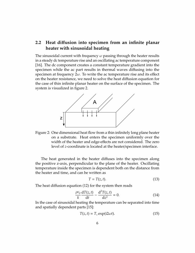
2.2 Heat diffusion into specimen from an infinite planarheater with sinusoidal heating

The sinusoidal current with frequency ω passing through the heater resultsin a steady dc temperature rise and an oscillating ac temperature component[16]. The dc component creates a constant temperature gradient into thespecimen while the ac part results in thermal waves diffusing into thespecimen at frequency 2ω. To write the ac temperature rise and its effecton the heater resistance, we need to solve the heat diffusion equation forthe case of thin infinite planar heater on the surface of the specimen. Thesystem is visualized in figure 2.

z

A

Figure 2: One dimensional heat flow from a thin infinitely long plane heateron a substrate. Heat enters the specimen uniformly over thewidth of the heater and edge-effects are not considered. The zerolevel of z-coordinate is located at the heater/specimen interface.

The heat generated in the heater diffuses into the specimen alongthe positive z-axis, perpendicular to the plane of the heater. Oscillatingtemperature inside the specimen is dependent both on the distance fromthe heater and time, and can be written as

T = T(z, t). (13)

The heat diffusion equation (12) for the system then reads

ρcp

kdT(z, t)

dt−

d2T(z, t)dz2 = 0. (14)

In the case of sinusoidal heating the temperature can be separated into timeand spatially dependent parts [15]:

T(z, t) = Tz exp(i2ωt). (15)

6

Plugging this into the heat equation, carrying out the differentiation withrespect to t and dividing by exp(i2ωt) yields

d2Tz

dz2 − i2ωα

Tz = 0 , (16)

where α is the thermal diffusivity, dimensions m2/s. Solution to the spatialpart inside the specimen, where z > 0, is

Tz = T0 exp(−qz), (17)

where q is the wavenumber of the thermal wave, defined as

q =√

i2ω/α = (1 + i)

√ωα

=

√2ωα· exp(iπ/4). (18)

Solution (17) vanishes at large z and yields the temperature of the heater T0

at z = 0. Now the time dependent periodic temperature inside the specimencan be expressed as

T(z, t) = T0 exp(i2ωt − qz). (19)

The heat flux into the specimen right at the heater/sample interface canbe written as [17]

φ∣∣∣z=0+ = −k

dT(z, t)dz

∣∣∣∣∣z=0+

= kqT0 exp(i2ωt)

= kT0

√2ω/α · exp(i2ωt + iπ/4). (20)

The flux equals the oscillating heat component produced in the heater perunit area. The oscillating power component of the heater is seen in equation(3). The oscillating power of the heater can be written in complex notation:

P0 cos(2ωt) = P0<(exp(i2ωt)

). (21)

Dividing the complex power by the heater area A and setting it equal to theheat flux from equation (20) gives

P0

Aexp(i2ωt) = kT0

√2ω/α exp(i2ωt + iπ/4). (22)

7

This yields us an expression for T0, the oscillative heater temperature:

T0 =P0

k√

2ω/αA· exp(−iπ/4) =

P0√2ωcpkA

· exp(−iπ/4). (23)

Now we can express the specimen temperature oscillations with explicitω-dependence:

T(z, t) = T0 exp(i2ωt − qz) =P0√

2ωcpkA· exp(i2ωt − iπ/4 − qz). (24)

Temperature lags the heater current by π/4 and has ω−1/2-dependence.Now we can calculate the effect of the oscillative heater temperature

to the heater resistance by using equation (5) and the real part of (24) justbelow the heater where z = 0.

R(t) = R0(1 + β∆Tdc + β∆Tac cos(2ωt + π/4)), (25)

where ∆Tdc is the dc temperature rise and ∆Tac is P0/A · (2ωcpk)−1/2, the peakamplitude of the ac temperature oscillations. The voltage across the RTDcan be obtained by multiplying the heater resistance with the input current,resulting in

V(t) = I0R0

((1 + β∆Tdc

)cos(ωt) +

12β∆Tac cos(ωt + π/4)

+12β∆Tac cos(3ωt + π/4)

). (26)

The 3ω and ω components in the voltage with phase shift result frommultiplying the 2ω term in the resistance with the input current oscillatingat the frequency ω. We can express the 3ω amplitude as

V3ω =12

V0β∆Tac, (27)

where V0 = I0R0. By measuring the voltage at the frequency 3ω one is ableto deduce the in-phase and out-of-phase components of the temperatureoscillations.

The finite thermal diffusion time τD of the specimen affects both themagnitude and the phase of the temperature oscillations. Required time

8

for the thermal wave to propagate a distance L in the specimen is given byequation

τD = L2/α , (28)

where α is the thermal diffusivity [18]. The angular frequency related tothe thermal diffusion is directly proportional to thermal diffusivity

ωD =2πτD

=2πα

l2 ∝ α. (29)

If the thermal diffusivity is infinite, no temperature gradients will form intothe specimen and there would be no phase lag between the driving currentand the temperature oscillations. At the limit of zero thermal diffusivitythere would be no heat propagation into the sample.

2.3 One-dimensional line heater inside the specimen

To calculate the thermal conductivity of the material under a line heater, onecan first study the simplified model of temperature oscillations a distancer = (x2 + y2)1/2 away from an infinitely narrow line source of heat on thesurface of an infinite half-volume.

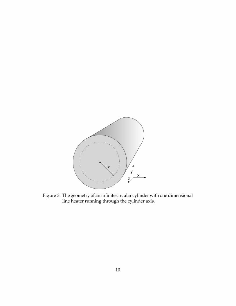
First the form of the temperature oscillations has to be solved for thecase of infinite volume. The solution can be found in for example Carslawand Jaeger [15] and their arguments are repeated here. Picture of thearrangement of the infinite case is shown in figure 3. Assuming that there isno axial or circumferential temperature gradients, the spatial heat diffusionequation for the temperature in the cylinder, T(r, t), can be written as

∂2T(r, t)∂r2 +

1r∂T(r, t)∂r

−1α

∂T(r, t)∂t

= 0. (30)

The temperature function can be divided into spatial and time dependentparts because the heating power is sinusoidal, as was the case for thecartesian system in the previous subsection.

T(r, t) = Tr exp(i2ωt). (31)

As previously, plugging this into the heat equation, carrying out thedifferentiation with respect to t and dividing by exp(i2ωt) yields

d2Tr

dr2 +1r

dTr

dr− i

2ωα

Tr = 0. (32)

9

r

yx

z

Figure 3: The geometry of an infinite circular cylinder with one dimensionalline heater running through the cylinder axis.

10

Here i2ω/α equals q2, the wavenumber of the thermal wave squared, foundin the previous subsection. Changing variables from r to y = qr yields

y2 d2T(y)dy2 + y

dT(y)dy

− y2T(y) = 0. (33)

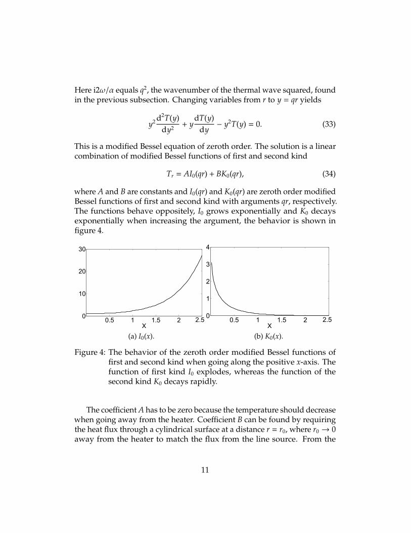
This is a modified Bessel equation of zeroth order. The solution is a linearcombination of modified Bessel functions of first and second kind

Tr = AI0(qr) + BK0(qr), (34)

where A and B are constants and I0(qr) and K0(qr) are zeroth order modifiedBessel functions of first and second kind with arguments qr, respectively.The functions behave oppositely, I0 grows exponentially and K0 decaysexponentially when increasing the argument, the behavior is shown infigure 4.

0.5 1 1.5 20

10

20

30

X

(a) I0(x).

0.5 1 1.5 2 2.50

1

2

3

4

X

(b) K0(x).

Figure 4: The behavior of the zeroth order modified Bessel functions offirst and second kind when going along the positive x-axis. Thefunction of first kind I0 explodes, whereas the function of thesecond kind K0 decays rapidly.

The coefficient A has to be zero because the temperature should decreasewhen going away from the heater. Coefficient B can be found by requiringthe heat flux through a cylindrical surface at a distance r = r0, where r0 → 0away from the heater to match the flux from the line source. From the

11

Fourier’s equation (7):

φ∣∣∣r=r0

= −kdT(r, t)

dr

∣∣∣∣∣r=r0

= −kBdK0(qr)

dr

∣∣∣∣∣r=r0

· exp(i2ωt)

= kqBK1(qr0) · exp(i2ωt), (35)

where K1 is a first order modified Bessel function of second kind. On theother hand, the heat flux from the heater through a cylindrical surface atr = r0 is

φ∣∣∣r=r0

= P/A =P0

2πlcylr0· exp(i2ωt). (36)

Equaling these we get the coefficient B:

B =P0

2kπlcylr0

1qK1(qr0)

. (37)

Series expansion for qr0K1(qr0) at r0 = 0 yields

qr0K1(qr0) = 1 + O(r20). (38)

This gives the expression for the spatial part of the temperature oscillations:

T(r) =P0

2kπlcylK0(qr). (39)

The total function for the temperature in the cylinder is then

T(r, t) =P0

2kπlcylK0(qr) · exp(i2ωt). (40)

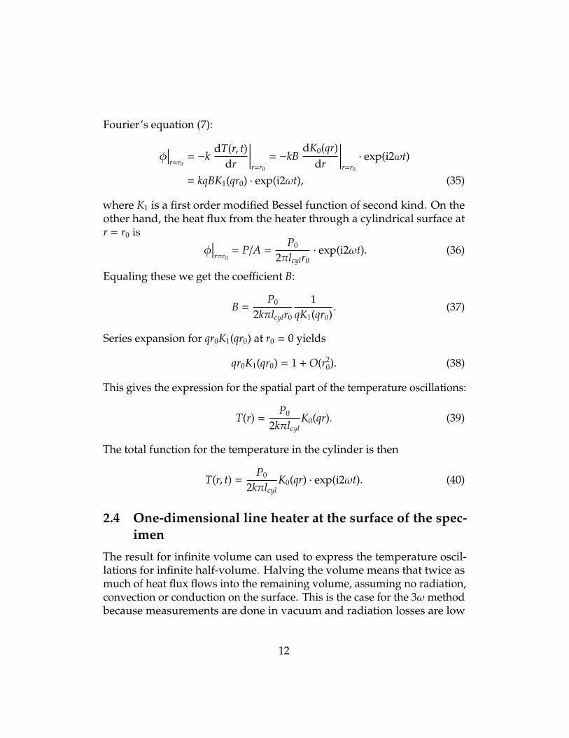
2.4 One-dimensional line heater at the surface of the spec-imen

The result for infinite volume can used to express the temperature oscil-lations for infinite half-volume. Halving the volume means that twice asmuch of heat flux flows into the remaining volume, assuming no radiation,convection or conduction on the surface. This is the case for the 3ω methodbecause measurements are done in vacuum and radiation losses are low

12

due to the rapid decay of the temperature oscillations [3]. Half-infinite caseis seen in figure 5. Equation (39) then becomes

T(r) =p0

πkK0(qr), (41)

and the total temperature function (40)

T(r, t) =p0

πkK0(qr) · exp(i2ωt), (42)

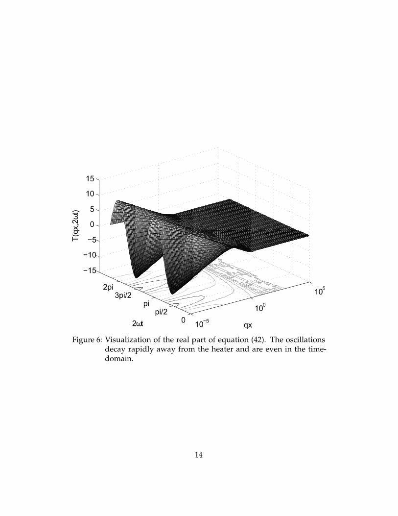
where p0 equals P0/lcyl, the heater power per unit length. The real part ofthe temperature function is visualized in figure 6.

r

yx

z

Figure 5: The geometry of a half-infinite circular cylinder with one dimen-sional line heater at the surface.

Even though the thermal oscillations decay rapidly because of the K0(qr),one has to make sure that the oscillations are contained inside the sample.This is done by calculating the penetration depth of the thermal wave inthe specimen. The thermal penetration depth λ relates to the wavenumberof the thermal wave q by

λ =1|q|

=

√α

2ω. (43)

Specimen can be considered semi-infinite if its thickness exceeds 5 thermalpenetration depths [3].

13

10−5

100

105

0pi/2

pi3pi/2

2pi

−15

−10

−5

0

5

10

15

qx2ωt

T(qx,2ωt)

Figure 6: Visualization of the real part of equation (42). The oscillationsdecay rapidly away from the heater and are even in the time-domain.

14

2.5 Finite heater width

Further, the heater in the experiment is not infinitely narrow but has a finitewidth. The effect of the finite width has to be taken into account in theanalysis. This is done by constructing the heater from infinite number of1D line heaters over the width of the heater [3]. This is visualized in figure7. Mathematically this is done by taking a Fourier transform of (41) withrespect to x-coordinate. Only the oscillations at the surface are important,so y = 0. Now Fourier cosine transformation can be used because thetemperature function is an even function. The Fourier cosine transformpair is:

f (η) =

∞∫0

f (x) cos(ηx)dx, (44)

f (x) =2π

∞∫0

f (η) cos(ηx)dη. (45)

For the spatial temperature oscillations the cosine transform reads [19]

T(η) =

∞∫0

T(x) cos(ηx)dx =p0

πk

∞∫0

K0(qx) cos(ηx)dx =p0

2k1√

η2 + q2. (46)

The finite width can be added into (46) by multiplying it with the Fouriertransform of the heat source as a function of the x-coordinate. Heat entersthe specimen evenly over the width of the heater ranging from −b to b. Thisbehavior can be expressed as a rectangular function with values 1 for x < |b|and 0 elsewhere. According to the convolution theorem, the multiplicationof the Fourier transforms of (46) and the rectangular function equals theFourier transform of the convolution of the functions in the x-space.

T(η) =p0

2k1√

η2 + q2

∞∫0

rect(x) cos(ηx)dx =p0

2ksin(ηb)

ηb√η2 + q2

. (47)

Inverse transform gives

T(x) =p0

πk

∞∫0

sin(ηb) cos(ηx)

ηb√η2 + q2

dη. (48)

15

b

(x1,y1) (xN,yN)

yx

Figure 7: The temperature inside the specimen at a certain point is result ofthe heat flow from all the one dimensional line sources that makeup a heater of finite width.

Equation (48) gives the form of temperature oscillations on the surface ofthe specimen a distance x away from the center of the heat source that has afinite width 2b. Since the thermometer and the heater are the same elementthe measured temperature is some average temperature over the width ofthe line. Expression (48) can be averaged by integrating it with respect tox from 0 to b and dividing by b to give the temperature measured by thethermometer:

Tavg =1b

b∫0

T(x)dx =p0

πk

∞∫0

sin2(ηb)

(ηb)2√η2 + q2

dη. (49)

Equation (49) is plotted in figure 8. The linear (on logarithmic scale)regime at the small frequencies is used to calculate the thermal conductivityof the specimen. The expression (49) cannot be solved in closed form, but atthe limit of large thermal penetration depth an asymptotic solution exists.To deem the thermal penetration depth large it has to be compared to theheater half-width b, which is in the same length scale [3]. When the heaterhalf-width b is much smaller than the thermal penetration depth λ, we canwrite

limb→0

sin(bη)(bη)

= 1. (50)

Values of η between λ < η < 1/b dominate the integral and the upper limit

16

can be set to 1/b [3]. After these, the expression can be approximated as

Tavg ≈p0

πk

1/b∫0

1√η2 + q2

dη =p0

πk

ln 1b

+

√1b2 + q2

− ln q

≈

p0

πk(ln 2 − ln(qb)

), (51)

where series expansion for the logarithm at b = 0 was used in the lastapproximation. It is more convenient to express this in terms of the thermalexcitation frequency 2ω, remembering that q = (1 + i)

√ω/α :

T(2ω) = −p0

2πk

(ln(2ω) + ln(b2/α) − 2 ln 2

)− i

p0

4k. (52)

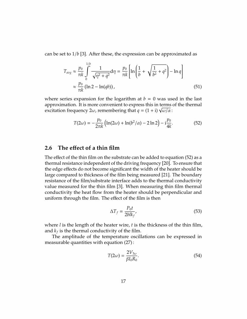
2.6 The effect of a thin film

The effect of the thin film on the substrate can be added to equation (52) as athermal resistance independent of the driving frequency [20]. To ensure thatthe edge effects do not become significant the width of the heater should belarge compared to thickness of the film being measured [21]. The boundaryresistance of the film/substrate interface adds to the thermal conductivityvalue measured for the thin film [3]. When measuring thin film thermalconductivity the heat flow from the heater should be perpendicular anduniform through the film. The effect of the film is then

∆T f =P0t

2blk f, (53)

where l is the length of the heater wire, t is the thickness of the thin film,and k f is the thermal conductivity of the film.

The amplitude of the temperature oscillations can be expressed inmeasurable quantities with equation (27) :

T(2ω) =2V3ω

βI0R0. (54)

17

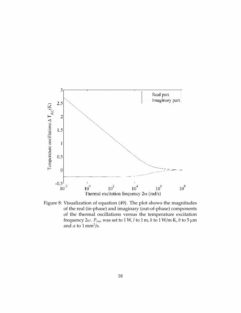
Figure 8: Visualization of equation (49). The plot shows the magnitudesof the real (in-phase) and imaginary (out-of-phase) componentsof the thermal oscillations versus the temperature excitationfrequency 2ω. Prms was set to 1 W, l to 1 m, k to 1 W/m·K, b to 5µmand α to 1 mm2/s.

18

Equations (52), (53) and (54) combine up into

T(2ω) = Ts + T f =2V3ω

βI0R0= −

P0

2πksl

(ln(2ω) + ln(b2/α) − 2 ln 2

)− i

P0

4ksl+

P0t2bk f l

, (55)

where the subscript s denotes the substrate. Thermal conductivity of thethin film from (53) can now be expressed as

k f =P0t

2bl(∆T − ∆Ts). (56)

The thermal response of the substrate Ts can be calculated directly fromequation (52) and subtracted from the measured ∆T. Thermal conductivityof the substrate can also be calculated from the slope of ∆T versus ln 2ω asonly the ln(2ω)-term has frequency dependence.

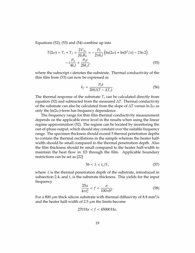
The frequency range for thin film thermal conductivity measurementdepends on the applicable error level in the results when using the linearregime approximation (52). The regime can be located by monitoring theout-of-phase output, which should stay constant over the suitable frequencyrange. The specimen thickness should exceed 5 thermal penetration depthsto contain the thermal oscillations in the sample whereas the heater half-width should be small compared to the thermal penetration depth. Alsothe film thickness should be small compared to the heater half-width tomaintain the heat flow in 1D through the film. Applicable boundaryrestrictions can be set as [22]

5b < λ < ts/5 , (57)

where λ is the thermal penetration depth of the substrate, introduced insubsection 2.4, and ts is the substrate thickness. This yields for the inputfrequency

25α4πt2

s< f <

α100πb2 . (58)

For a 800 µm thick silicon substrate with thermal diffusivity of 8.8 mm2/sand the heater half-width of 2.5 µm the limits become

270 Hz < f < 45000 Hz.

19

3 Experimental Methods

3.1 Overview

Materials used in the heater fabrication for the 3ω method have includedfor example gold, aluminum, and silver [3, 23]. These materials have largeenough temperature coefficients of resistance to create a measurable 3ωvoltage signal. Gold and bismuth were used in the experiments of this work.Bismuth was chosen because the resistivity of thin films has good responseto temperature changes also at low temperatures [24]. The resistivity ofbulk bismuth, 1.29 µΩm, is high compared to traditional heater metals likegold with 22.14 nΩm and silver, 15.87 nΩm, all the values at 20 °C [25].Thin bismuth films have negative TCR [24], whereas the previous studieshave used heater materials with positive coefficients [3, 21, 12].

Figure 9: SEM image of a bismuth heater/thermometer deposited on SiOx.The length of the line is 1 mm and the width is 10 µm.

20

3.2 Sample fabrication

The films used in the experiments were vacuum deposited on thermallyoxidized boron doped silicon substrates. Oxide thickness of the films wasmeasured with Rudolph AUTO EL III ellipsometer and found to be around300 nm. To achieve optimal thermal contact between the heater and thesubstrate the chips were cleaned by sonicating them in hot acetone for 1− 2minutes. After the sonication the chips were rinsed with isopropyl alcohol(IPA) to remove the acetone residue and blow dried with nitrogen.

(a) Coat and bake copolymer resist. (b) Coat and bake PMMA.

(c) Exposure. (d) Development.

(e) Metal evaporation. (f) Lift-off.

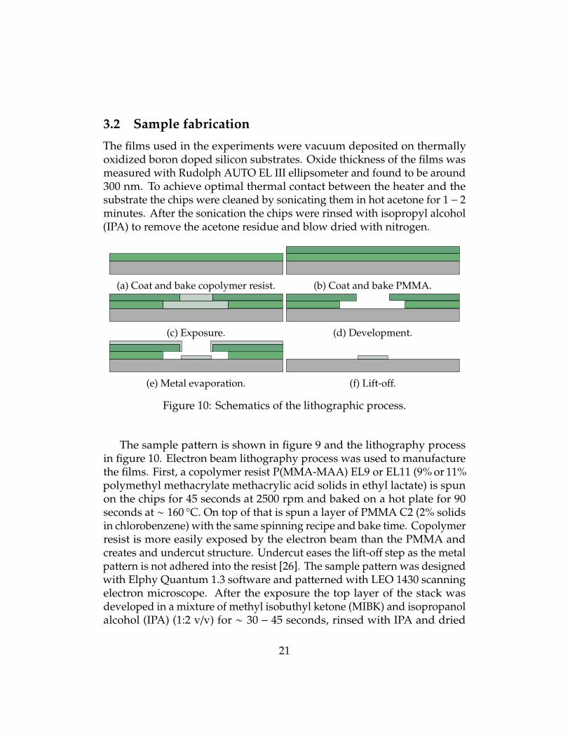
Figure 10: Schematics of the lithographic process.

The sample pattern is shown in figure 9 and the lithography processin figure 10. Electron beam lithography process was used to manufacturethe films. First, a copolymer resist P(MMA-MAA) EL9 or EL11 (9% or 11%polymethyl methacrylate methacrylic acid solids in ethyl lactate) is spunon the chips for 45 seconds at 2500 rpm and baked on a hot plate for 90seconds at ∼ 160 °C. On top of that is spun a layer of PMMA C2 (2% solidsin chlorobenzene) with the same spinning recipe and bake time. Copolymerresist is more easily exposed by the electron beam than the PMMA andcreates and undercut structure. Undercut eases the lift-off step as the metalpattern is not adhered into the resist [26]. The sample pattern was designedwith Elphy Quantum 1.3 software and patterned with LEO 1430 scanningelectron microscope. After the exposure the top layer of the stack wasdeveloped in a mixture of methyl isobuthyl ketone (MIBK) and isopropanolalcohol (IPA) (1:2 v/v) for ∼ 30 − 45 seconds, rinsed with IPA and dried

21

with nitrogen. The bottom layer was further developed in a 1:2 v/v mixtureof 2- methoxyethanol and methanol for ∼ 5 seconds, rinsed with IPA anddried in nitrogen flow.

The gold films were evaporated with a custom-made ultra-high vacuume-beam evaporator at a rate of 2 nm/s. A 15 nm titanium layer was usedas an adhesion layer for the gold heater. Bismuth was evaporated byBalzers BAE 250 vacuum e-beam evaporator at a base pressure of ∼ 5 mbar.Bismuth used for the films is 99.9999% pure, obtained from Goodfellow Inc.Evaporation rate was around 2 nm/s. The lift-off was done in hot acetone,with a brief sonication if necessary. After the lift-off the chips were rinsedwith IPA and dried.

3.3 Measurement setup

The schematics of the measurement setups are shown in figures 11 and 12.Stanford Research Systems SR830 lock-in amplifier is used to supply thefundamental sinusoidal heater voltage and to read the ω and 3ω signals.

In the first setup the current bias is achieved by using a load resistor R0

in series with the sample, 10 kΩ for gold samples and 100 kΩ for bismuth.Voltage drop across the sample is measured differentially with the lock-inamplifier, both the 3ω and the fundamental 1ω voltages are measuredsimultaneously by using separate lock-in amplifier to read the differentharmonics. The fundamental signal is fed as the reference signal to both ofthe lock-in amplifiers. Temperature of the sample stage is measured with aPt100 resistance thermometer by reading its resistance with AVS resistancebridge.

The second approach involves a Wheatstone bridge to extract the 3ωvoltage originating from the sample, as shown in figure 12. Resistor R2

is one hundred times larger than R1 to get almost all of the current passthrough the sample resistance Rs. With the bridge setup it is possible toincrease the resistive heating of the metal line as more current can be passedthrough it. The bridge is balanced by tuning the variable resistor Rv andmonitoring the voltage between the bridge arms by SR830 lock-in amplifier.The 3ω output of the balanced bridge W3ω is related to V3ω of the sample by

W3ω =R1

Rs + R1V3ω,

22

Sample

Vacuum chamberR0

Lock-inamplifier

Signal in

Temperature

Lock-in amplifier

V

Sine out

Reference in

Read-out

Figure 11: Schematic of the measurement setup. Two lock-in amplifiersmake it possible to read the fundamental 1ω voltage and the 3ωvoltage simultaneously.

23

V0 W3w

Rv

R2R1

Rs

Figure 12: Schematics of the Wheatstone bridge measurement setup. SR830lock-in amplifiers were used to supply the fundamental voltageand to read the 3ω response.

where Rs is the room temperature resistance of the sample and R1 is theresistance of the in-series resistor [27].

3.4 Measurements

The 3ω measurements were performed at room temperature and aboveby using a custom compiled measurement instrumentation. A picture ofthe vacuum chamber, the electrical feedthrough and the sample stage isseen in figure 13. The samples were mounted on the sample stage withsilver paint to ensure good thermal contact and easy removal. Electricalcontacts for the gold samples were made with Kulicke & Soffa 4523A wirebonder with Al-wire. For bismuth samples the electrical contacts weremade by melting a piece of indium into the tip of a wire and pressing it tothe bonding pad with a scalpel tip. The bonding pads were made large forthis reason. This approach is required because bismuth is a soft materialand traditional ultrasonic bonding does not work properly on it. The Pt100resistance thermometer was mounted on the stage with thermal grease tomeasure the temperature of the system. The sample stage was inserted

24

Figure 13: The vacuum chamber with the electrical feedthrough and thesample stage.

25

into a vacuum chamber to minimize the heat loss to the surroundings. Avacuum of 10−3

− 10−4 mbar was achieved with a diffusion pump.Measurement data were collected with a custom LabVIEW virtual

instrument capable of handling all the necessary input channels at thesame time. The temperature coefficient of resistance of the metal linewas measured prior to the 3ω measurements. The vacuum chamber washeated up to 40 °C by blowing hot air into the walls with a hot-air gun.Temperature response of the heater voltage was then measured duringthe cooling of the vessel back to the room temperature. Small amplitudesignal of 0.1 V rms with 100 Hz frequency at lock-in output was used toavoid resistive heating of the metal line. A 100 kΩ resistor in series withthe sample was used to limit the current in the circuit. Temperature of thestage was simultaneously measured with the Pt100 to fix the heater data ona temperature scale.

Actual 3ω measurements were performed at room temperature orduring the cooldown after heating. Frequencies were scanned between100 − 1000 Hz at 100 Hz intervals with a LabVIEW instrument speciallymade for this purpose. Each frequency was maintained for 10 seconds tostabilize the readings. However, the requirement of the stable readings ledinto measurement times being over 2 minutes and the temperature of thesample stage decreased by multiple degrees during the frequency sweepfrom 100 to 1000 Hz. Maintaining stable temperature with the hot-air gunproved to be challenging and so the measurements were performed nearthe room temperature where the temperature change of the sample stagewas negligible. The magnitude of the driving current was set so that theamplitude of the 1ω voltage was approximately 10000 times larger thanthe 3ω voltage. At this ratio the fluctuations of the output signal remainedmoderate so that the measurements could be performed.

The manual bonding method of the electrical contacts into bismuthsamples turned out to be problematic. Most of the contacts made intothe films did not survive long enough for he measurement cycles to beperformed. Some contacts were lost by accidentally heating the specimenvessel too much and thus melting the indium contacts. The failing of theelectrical contact between the wire and the bismuth pads was observed asincreasing of the sample resistances.

26

4 Results

The temperature coefficient of resistance of the metal heater was obtainedby linear regression from the measured temperature response. For bismuthan example is shown in figure 14 and for gold in figure 15. Resistance ofthe heater was obtained from the fundamental 1ω voltage measured overthe heater. The value of the TCR is obtained by dividing the slope of thetemperature response of the metal line with the heater resistance at ambienttemperature. For bismuth lines the TCR values are around 2 · 10−3 1/K andfor gold lines around 3 · 10−3 1/K.

302 303 304 305 306 307 308 309 310 311 312

2330

2340

2350

2360

2370

2380

Data points Linear fit y = a + bx

b = -5.88579 0.01111 /K

Res

ista

nce

()

Temperature (K)

Figure 14: Resistance of a 5 µm wide and 300 nm thick bismuth line versustemperature near the room temperature. Step-like behavior isdue to insufficient resolution.

The error in the temperature oscillations of the specimen builds upmostly from the error in TCR measurement and the fluctuations in theoutput of the 3ω voltage. Possible error sources can be seen in equation(54), V3ω and the TCR dominate the error. The linear fit into heater datafor TCR is accurate, some error may arise from the lag between the heaterand the Pt100 sensor. If the response time of the Pt100 is multiple seconds

27

300 301 302 303 304 30512.40

12.42

12.44

12.46

12.48

12.50

12.52

12.54

12.56

12.58

12.60

Data points Linear fit y = a + bx

b = 0.03388 ± 2.07787E-5 Ω/K

Res

ista

nce(

Ω)

Temperature(K)

Figure 15: Resistance of a 10 µm wide and 250 nm thick gold line versustemperature near the room temperature.

behind that of the metal line the temperature scale of the linear fit is off bysome degrees. The measured temperature response of the metal lines ishowever linear over a range of 10 degrees so a lag of some degrees wouldnot affect the value of TCR.

Measured 3ω voltages for a 5 µm wide and 300 nm thick bismuthheater are seen in table 1. Temperature oscillations in the substrate arecalculated from equation (52). Values used for thermal conductivity andthermal diffusivity of the silicon substrate are 149 W/m·K and 8.8 · 10−5

m2/s, respectively [25]. The values measured with the setup of figure 11 areseen in table 1 along the results for the measured temperature oscillations,the measured temperature oscillations in the thin film and the calculatedthermal conductivity of the film. The thermal conductivity of the silicondioxide film is calculated with equation (56), the film thickness set to 300nm. Results for a 10 µm wide and 250 nm thick gold heater measured withthe setup of figure 11 are seen in table 2.

The calculated values for temperature oscillations in the substrate aresmall when compared into values reported earlier [23, 20]. The oscillations

28

Table 1: Output data for a 5 µm wide and 300 nm thick bismuth heater. Thedriving frequency and the corresponding temperature oscillationsof the whole specimen, the film, and the substrate plus the thermalconductivity of the thin film. Measurement was done with 0.75 Vinput voltage to get a well reacting 3ω output. The heater powerper unit length is 121 µW/m.

f (Hz) V3ω (µV) ∆T (K) ∆Ts (µK) ∆T f (K) k f (W/m·K ·10−5)100 2.77 0.140 1.52 0.140 5.18200 2.80 0.142 1.42 0.142 5.13300 2.79 0.141 1.37 0.141 5.14400 2.81 0.142 1.33 0.142 5.11500 2.81 0.142 1.30 0.142 5.12600 2.84 0.144 1.27 0.144 5.06700 2.85 0.144 1.25 0.144 5.05800 2.89 0.146 1.24 0.146 4.98900 2.88 0.145 1.22 0.145 5.01

1000 2.88 0.145 1.21 0.145 5.01

Table 2: Output data for a 10 µm wide and 250 nm thick gold heater. Thedriving frequency and the corresponding temperature oscillationsof the whole specimen, the film, and the substrate plus the thermalconductivity of the thin film. Measurement was done with 3.156 Vinput voltage to get a well reacting 3ω output. The heater powerper unit length is 1.4 mW/m.

f (Hz) V3ω (µV) ∆T (K) ∆Ts (µK) ∆T f (K) k f (W/m·K ·10−5)100 4.26 0.703 16.8 0.703 5.98200 4.21 0.693 15.6 0.693 6.06300 4.23 0.697 14.9 0.697 6.02400 4.21 0.694 14.4 0.694 6.05500 4.24 0.699 14.0 0.699 6.00600 4.25 0.701 13.7 0.701 5.99700 4.25 0.700 13.4 0.700 6.00800 4.22 0.695 13.2 0.695 6.04900 4.23 0.698 13.0 0.698 6.02

1000 4.31 0.710 12.8 0.710 5.91

29

in the substrate should be of the same order of magnitude as the totaloscillations. The error in the measurement causes the calculated thermalconductivity of the silicon dioxide film to be 5 orders of magnitude off froman acceptable value about 1.3 W/m·K [23, 20]. The expected 3ω output of themeasurement can be calculated when the film thermal conductivity is fixedto 1.3 W/m·K. The values obtained from equation (55) give values around1 − 2 · 10−10 V. Measurements performed with the Wheatstone bridge setupwere unsuccessful. The circuit did not give reasonable readings for the 3ωvoltage over the bridge. This is probably due to third harmonic noise fromthe components or the signal sources that were used in the setup.

The vacuum does not affect the output value of the 3ω signal. This is notdesired behavior as the heat generated in the metal line should be conductedinto the surrounding air when measuring in atmospheric pressure. Thereason behind this is probably the noise in the circuit. The out-of-phasesignal, which can be used to locate the linear regime [3], did not show anylinear behavior. The signal was however smaller than the in-phase signalby a factor of ten, which is somewhat proper behavior. Fluctuations in boththe magnitude and the phase of the out-of-phase signal were unpredictableand the identification of the linear regime based on the out-of-phase outputproved implausible.

30

5 Conclusions and Future Work

The goal of validation of the 3ω method for thermal conductivity measure-ments was not achieved. Obtained 3ω signal did not contain informationabout the thermal properties of the measured samples. At first this wasthought to be due to low power level in the metal line heater, but furthermeasurements with the Wheatstone bridge setup suggest that the cause isspurious 3ω signals from the components. The actual source of this signalremains unknown.

If the 3ω measurements are further pursued the measurement setupshould be rebuilt keeping in mind the requirement of accurate temperaturecontrol of the stage and high enough power in the metal line heater. Fortemperatures lower than room temperature a dipstick with vacuum wouldbe optimal. Raising the dipstick from liquid helium or liquid nitrogenprovides slow and controllable rate of temperature change and accuratemeasurements at precise temperatures would be possible. A standardizedspecimen mount with connections to the dipstick would ease the problemswith the electrical connections to the sample.

A more sophisticated LabVIEW instrument to sweep frequencies atsmaller intervals than 100 Hz would ease the locating of the linear regime.At one frequency step the instrument should record the in-phase 1ω and3ω voltages over the sample plus the out-of-phase 3ω signal with the phaselag. For SR830 GPIB bus can be used to command the lock-in amplifier tochange the signal frequency and the channel output. A possible problemmay arise from the lock-in amplifier’s limited output signal magnitude. Acommon multimeter can be used to monitor the 1ω voltage if the outputrange of the lock-in amplifier is exceeded. Temperature measurementsbelow −200 °C require a temperature probe other than Pt100.

31

References

[1] D.G. Cahill et al., J. Appl. Phys. 93 (2003) 793.

[2] W.S. Capinski et al., Phys. Rev. B 59 (1999) 8105.

[3] D.G. Cahill, Rev. Sci. Instrum. 61 (1990) 802.

[4] O.M. Corbino, Phys. Z. 11 (1910) 413.

[5] O.M. Corbino, Phys. Z. 12 (1911) 292.

[6] L.R. Holland, J. Appl. Phys. 34 (1963) 2350.

[7] D. Gerlich, B. Abeles and R.E. Miller, J. Appl. Phys. 36 (1965) 76.

[8] L.R. Holland and R.C. Smith, J. Appl. Phys. 37 (1966) 4528.

[9] N.O. Birge and S.R. Nagel, Phys. Rev. Lett. 54 (1985) 2674.

[10] N.O. Birge and S.R. Nagel, Rev. Sci. Instrum. 58 (1987) 1464.

[11] D.G. Cahill and R.O. Pohl, Phys. Rev. B 35 (1987) 4067.

[12] S.M. Lee, D.G. Cahill and T.H. Allen, Phys. Rev. B 52 (1995) 253.

[13] G. Gesele et al., J. Phys. D 30 (1997) 2911.

[14] X.J. Hu et al., J. Heat Transfer 128 (2006) 1109.

[15] H. Carslaw and J. Jaeger, Conduction of heat in solids (ClarendonPress, 1959).

[16] K. Banerjee et al., Reliability Physics Symposium Proceedings, 1999.37th Annual. 1999 IEEE International, pp. 297 –302, 1999.

[17] U.G. Jonsson and O. Andersson, Meas. Sci. Technol. 9 (1998) 1873.

[18] N.O. Birge, Phys. Rev. B 34 (1986) 1631.

[19] A. Erdélyi, Tables of Integral Transforms (McGraw-Hill, 1954).

[20] S.M. Lee and D.G. Cahill, J. Appl. Phys. 81 (1997) 2590.

32

[21] D.G. Cahill, M. Katiyar and J.R. Abelson, Phys. Rev. B 50 (1994) 6077.

[22] D. de Koninck, Thermal conductivity measurements using the 3-omegatechnique: Application to power harvesting microsystems, Master’sthesis, Department of Mechanical Engineering, McGill University,Montréal, Canada, 2008.

[23] T. Yamane et al., J. Appl. Phys. 91 (2002) 9772.

[24] R.A. Hoffman and D.R. Frankl, Phys. Rev. B 3 (1971) 1825.

[25] W. Haynes and D. Lide, CRC Handbook of Chemistry and Physics: AReady-Reference Book of Chemical and Physical Data .

[26] MicroChem PMMA Data Sheet, http://microchem.com/pdf/PMMA_Data_Sheet.pdf, Accessed 12/2012.

[27] N.O. Birge, P.K. Dixon and N. Menon, Thermochim. Acta 304–305(1997) 51 .

33