'1

~ I

I

~

I.,

I

JOURNAL OF RESEARCH of the Notional Bureau of Standards Vo lume 83, No. 4, July- August 1978

Implementation of Scaling and Extended Scaling Equations of State for the Critical Point of Fluids

M. R. Moldover

National Measurement Laboratory, National Bureau of Standards, Washington, D. C. 20234

February 21, 1978

An ex plicit , practical procedure is suggested for transforming from the laboratory va ri ables densit y (p) and

tempe rature (1' ) into the parametri c vari ables r and 0, which occur in various sca led representati ons of equ ati ons

of s tate and of transport prope .1ies of fluids near critica l po int s. A reasonabl y effi cient and versati le computer

p rogra m illustratin g thi s proced ure is prov ided. With thi s program, the para me tri c equa ti ons of state whi ch occur

in seve ra l formul ations of simple, exte nd ed , and/or revi sed sc<:ding a re as easy 1. 0 use as a ny other equ ati on of Sl aLe

for whi ch T a nd p are the independent variab les.

Key words: Critical point; equation of state; sca ling eq uation of s tate.

1 . Introduction

In recent years various scaling eq uations of state have been developed to provide theore tically based , highl y accu­rate representatio ns of thermod ynamic data for pure fluids and fluid mixtures near their c ritical points. These equations of state are all consistent with the hypothesis that very near the c ritical point the thermodynamic pote ntial is a homoge­neous function of its natural variables. These equations of state have relativ e ly few parameters which must be adjusted to fit data for any specifi c fluid . This is a practi cal advantage for those concerned with taking or correlating data. On the other hand, man y scaling equations of state are written in terms of parame tric variables which appear in nonlinear equations linking together such physically relevant variables as the pressure (P ), the density (p), and the temperature (T). The OCCUlTence of the parametric variables is a major practical disadvantage to any nonexpert who might otherwise be interested in us ing a scaling equation of state to deal with a limited problem. It is, of course, true that these parametric variables can be eliminated algebraically from the equation of state along special paths in thermod ynamic space such as the vapor pressure curve. Then, along the spec ial paths, the scaling equations reduce to simple power laws with noninte­gral exponents re lating directly measured quantities to each other. For states off these special paths, a user of a scaling equation of state must eliminate the parametri c variables numerically. The purpose of the present paper is to provide an explicit example of one way in which this can be done. If our method is foDowed , a user need not repeat the program­ming effort required to eliminate the parametric variables in

1 Figures in brackets indicate literature references at the end of the paper.

those situations in which p and T are independent variables. In s itutations in which it is conveni ent to des ignate other physical variables as independent, the genera l method out­lined here may still be followed.

In this work we discuss onl y those scaling equations of state which use parametric variables. There a re several published exam ples of scaling equations of s tate which do not use parametri c variables [1 ,2]. I Unfortunately, these non-parametric equations of state cannot be integrated in closed form to obta in an explic it express ion for the thermo­dynamic potential. Thus, frequentl y used expressions for the ent ropy and for the specific heats consistent with non­parametric equa tions of state contain integrals which must be evaluated nume rically. In our experi ence, the lac k of an explicit thermodynamic potenti al has been a se rious handi­cap in attempting to use these non-parametri c eq uations for constructing thermodynamic models for real fluid s. Accord­

ingly, we now choose to deal with the numerical problems arising from the use of parametric variables rather than the numerical problems associated with integral representations for the potential.

2. Simple Scaling with the Linear Model

We will consider first the " linear model" parametric equation of state proposed by Schofield [3]. This equation was first proposed on phenomenological grounds and was applied with success to the insulating ferromagnet CrBra [4]. It has since received some theoretical justification [5] and it has been widely used to cOlTelate equation of state and transport property data in various fluid systems [6-9]. Most important from our present point of view, the equations to be solved in using the linear model parametric equation of state

329

may be easily generalized to handle the more complicated cases of extended and/or revised scaling.

To use the linear model parametric equation of state in si tuations where the temperature (T) and the density (p) are the independent variables, the parametric variables rand () must be obtained by solving the following two equations:

implement because the derivative , f' (Z), may be calculated analytically. In Newton's method , the (n + l)'th estimate for Z is found from the n' th estimate by the rule

(8)

(1) In the present case this rule takes the form

P = Pc + pcmrIJ () (2)

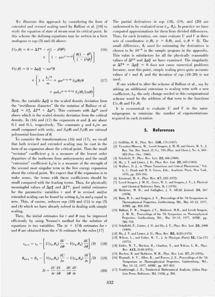
Here Tc and Pc are critical constants. For the simple fluids studied by Levelt Sengers et aI. , [7] m is a positive constant in the range 1. 5 < m < 2.1; b2 is a constant falling in the range 1.1 < b2 < 1.6, and the exponent {3 usually falls in the range 0. 31 < {3 < 0 .38. The transformation represented by eqs (1) and (2) for the fluid xenon is ske tched in figure 1. To make this sketch , values of T c, Pc, m, and b2 were taken from reference [7] . Once values of rand () are obtained by solving (1) and (2), other quantities such as the pressure (P) and the constant volume specific heat (C v) may be calculated as functions of p and T by simply substituting r and () into algebraic equations which can be solved explicitly for the desired quantities [7 ,10]. There are many ways to solve these equations numerically. The method described here is reasonably efficient and reliable.

To solve (1) and (2) we first introduce the dimensionless variables I1T* = (T - Tc)/ Tc, and I1p* = (p - Pc)/ Pc to obtain

(3)

o = I1p* - mrIJ() (4)

We then eliminate r from (1) and (2) to obtain

Note that absolute value signs had to be introduced because we have chosen to raise to powers the separate quantities I1T* and (1 - b2(J2) rather than their quotient which always re mains positive. By introducing two new symbols, Z and C

Z = be (6)

b C = -l1p* - II1T* I-IJ

m we obtain a compactly written transcendental eq uation in one variable

feZ) = 0 = C + Z 11 - Z2 I -IJ (7)

Z = Z _ (1 - Z~)(Zn + C nil - Z~ I IJ) n+1 n (1 - Z~) + 2{3Z~ (9)

Equation (9) is quite satisfactory for computation if suitable precautions are taken to handle the singularity at Z = 1. Each iteration requires only a single exponentiation . A reasonable initial estimate for Z is obtained by looking at the

... II: => .... ..:

300

~ 280 0-

:IE ... ....

260

o

0 =-0 .766 0 =0

, ... ,=0.05

" , \

\ \

\

• .. _' • 1000

DENSITY (kg /m3,

0=0.766

\

2000

FIGURE 1. Sketch of the transformation from p and T to rand (J in the

linear model (eqs (1) and (2)) with parameters appropriate for xenon from reference [7).

physically important special curves, namely: the critical isochore above T c for which Z = 0, the cri tical isotherm for which Z = ± 1 and finally or coexistence curve on which Z = + b in the liquid phase and Z = - b in the vapor phase.

Numerical approximations to its roots may be found effi- An estimate which has the appropriate limits near the special cientl y by Newton's method. This is particularly easy to curves I S :

330

~

I

r ;

l rl

(1 - b)t.. T* I m ! 1/13 Z = 1 - - for t..T* < 0 o 1 - b2 t..p*

1m 1

1/13 Zo = (1 + t..T* bt..p* )-13 for t..T* > 0

(10)

We have applied this approach to the solution of eqs (3) and (4) with the double precision Fortran program listed in appendix I. For all of the physically reasonable values of input parameters we have tried, at mos t five iterations were needed. The resulting values of r and 8 satisfy eqs (3) and (4) to 12 or more significant figures. (When It..p*1 and/or It..T*1 are small el- than 10- 12 , an " unphysical" situation, the sample program yields fewe r s ignificant fi gures) . If a sub­stantial amount of computation were to be done with a single value of {3, a program could be written in which the time­consuming step of ra ising a floatin g point number to a fl oating point power occurs Jess frequentl y than the 2-7 times it occurs with the present program .

In concluding thi s section we note that solutions to (3) and (4) in the range 1 < ()2 < I/W(l - 2(3)] may be interpreted as ei ther two phase states (for which 8 should be set to ± 1) or metas table exte nsions of the single phase isotherms [11]. Very little is known about the accuracy of the linear model when it is used in the metastable region.

3. Additional Examples Using Simple Scaling

Other familiar parametric vers ions of simple scaling can be handled in the same way as the " linear mod el" . For example, the "cubic model" introduced by Ho and Litste r [12] uses two parametric variables which may be considered to be defined by the equations:

(11)

(12)

Again we have used rand 8 as the parametric variables while m, b, (3 , and C2 are constants. If the same substitutions are made in (11) and (12) as those used above in connection with the linear model , one may obtain:

feZ) = 0 = C + z(l + :! Z2) 11 - z21-13 (13)

In practice, C2 Z/b2 is much less than unity so that (13) is very similar to (7) . Initial estimates for the solution to (13) may be obtained from eq (10), just as for the "linear model"; then the solution by Newton's method proceeds exactly as outlined above except that the "cubic model" function for j(Z) is used instead of the linear model function.

A parametric scaling equation of state was introduced by Wilcox and Es tler [13] to deal with data from diffraction experiments in fluid s near c ritical points. Their scheme has been used by Estl eI' e t al. [14] and by Hocken and Moldover [IS]. For a given fluid state, the parametric variables in the Wilcox-Estl eI' sche me have numerical values wh ich are quite different from those which appear in the " linear model" or the "cubic model". One may consider the variables to be defin ed by the equations:

0= I t..p* I - [YoR(1 - 8/ ( 0 )6] 13 (14)

X 1 + - ----'---'" [ {31 - 8/ 8x] y 1 - 8/80

o = t..T* - R8 (15)

Here, following Wilcox and Estl e r, the parametric va ri ables are "R" and "8" whil e Yo, 80 , 8x, {3 and yare all consta nts, and t.. is a combination of constants: t.. = 1 - 8J 8x. (Note: Because the absolute value of t..p* appea rs in (14), the inverse transformation from R and 8 to t..p* and t..T* is not unique). Once aga in one of the parametric variables, say R, may be eliminated from (14) and (15) to yield an equation in one variable which may be solved by New ton's method.

On occasion , T and p are not the most convenient independent variables. For example, the anal ys is of fl ow calorimetry data [16] requires the computation of the en­thalpy as a fun ction of T and P. Each of the s imple scaling equations of state mentioned above will lead to two eq uations relating P and T to parametric variables. The nume ri ca l problem of solving these equations for rand 8 is quite similar to the problem we have di scussed above, namely of solving the equations in p and T for r and 8. In particular, when P and T are known it is still possible to eliminate one of the parametric variables from the two equations algebraically. Thus a single equation in one unknown remains which may be effi c iently solved with Newton's method.

4. Extended and/or Revised Scaling

In more compli cated versions of scaling, the convers ion

from the labora tory variables p and T to the parametric vari ables r and 8 requires the numerical solution of two simultaneous equations. One parameter can no longer be eliminated algebraically. An efficient and versati le approach is to use simple scaling to obtain a first approximation to the values of the parametric variables . The approximation may then be improved by using Newton's method for the solution of simultaneous equations.

The same firs t approximation (simple scaling) may be used with a variety of more complicated models. Where the derivatives required for the use of Newton's method are computed numerically, it becomes quite easy to change from one model to another.

331

We illustrate this approach by considering the form of extended and revised scaling used by Balfour et al. [10] to stud y the equation of state of steam near its critical point. In this scheme the defining equations may be written in a form analogous to eqs (3) and (4) above:

k{t. + - + qarl - a - f3 So(e)/e

m

+ qak1r1- a -/3+t. SI(e)/(me)}

(16)

(17)

Here, the variable I1p~ is the scaled density deviation from the "rectilinear diameter" (In the notation of Balfour et al. Ap~ = A tl AT* + Ap*). This contrasts with Ap* used above which is the scaled density deviation from the critical density. In (16) and (17) the exponents a and 11 are about 0.1 and 0.5, respectively. The constants q and k tim are small compared with unity, and So(e) and SI(e) are rational polynomial functions of e.

To consider the transformations (16) and (17), we recall that both revised and extended scaling may be cast in the form of an expansion about the critical point. Thus the small "revision" coeffi cient q is a measure of the lowest order departure of the isotherms from antisymmetry and the small "extension" coeffic ient k l / m is a measure of the strength of the second most singular term in the free energy expansion about the critical point. We expect that if the expansion is to make sense, the te rms with these coefficients should be small compared with the leading terms. Thus, for physically meaningful values of Ap~ and I1T* , good initial estimates for the parametric variables rand e in revised and/or extended scaling can be found by setting kl / m and q equal to zero. This, of course, reduces eqs (10) and (11) to eqs (3) and (4) which we have already solved in dealing with simple scaling.

Then, the initial estimates for rand e may be improved efficiently by using Newton's method for the solution of equations in two variables. The (n + 1)'th estimates for r and e are obtained from the n'th estimate by the rules [17]

(18)

(19)

au av au av D= -- ---

ar ae ae ar (20)

The partial derivatives in eqs (18), (19), and (20) are understood to be evaluated near (r m en). In practice we have computed approximations for them from divided differences. Thus, for each iteration, one must evaluate U and V at three sets of coordinates: (r,e), (r + 8,e), and , (r,e + 8) . The small difference, 8, used for estimating the derivatives is chosen to be 10- 8 in the sample program in the appendix. This value is satisfactory for all the physically reasonable values of AT* and Ap~ we have examined. The singularity at AT* = Ap~ = 0 does not cause numerical problems because, near this point , simple scaling gives quite accurate values of rand e, and the iteration of eqs (18-20) is not used.

If one wished to alter the scheme of Balfour et aI., say by adding an additional extension to scaling term with a new coefficient, k2' the only change needed in this computational scheme woud be the addition of that term to the functions U(r, e) and V(r ,e).

It is economical to evaluate U and V in the same subprogram to minimize the number of exponentiations required in each iteration.

S. References

[1] Griffiths, R. B. , Phys. Rev. 158, 176 (1967). [2] Vicentini-Missoni, M., Levelt Sengers, J. M. H. and Green, M. S., J.

Res. Nat. Bur. Stand. (U.S.), 73A (Phys. and Chern.) , No.6, 563-583 (Nov.-Dec. 1969).

[3] Schofield, P. , Phys. Rev. Lett. 22,606 (1969). [4] Ho, J. T. and Litster, J. D., Phys . Rev. Lett. 22,603 (1969). [5] Wallace, D. J. , in "Phase Transitions and Critical Phenomena," Vol.

6, C. Domb and M. S. Green, Eds. , Academic Press , New York , 1976, pp. 293-356.

[6] Kierstead, H. A., Phys. Rev. A7, 242 (1972). [7] Levelt Sengers, J. M. H. , Greer, W. L. and Sengers, J. V. , J. Physical

and Chemical Reference Data, S, 1 (1976). [8] Moldover, M. R., and Gallagher, J. S. AIChE Journal , 24, 267

(1978). [9] Basu, R. S., and Sengers, J. V. , Proceedings of the 7th Symposium on

Thermophysical Properties, Gaithersburg, Md., May 10-12, 1977, ASME. pp. 822-830.

[10] Balfour, F. W., Sengers, J.V., Moldover, M.R., and Levelt Sengers, J. M. H., Proceedings of the 7th Symposium on Thermophysical Properties, Gaithersburg, Md. , May 10-12, 1977, ASME. pp. 786-793.

[11] Schofield, P., Litster, J. D. and Ho, J. T., Phys. Rev. Lett. 23, 1098

(1969). [12] Ho, J. T. and Litster, J. D., Phys. Rev. 82,4523 (1970). [13] Wilcox, L., and Estler, W. T., J. de Physique (Paris) 32, C5a-175

(1971). [14] Estler, W. T., Hocken, R., Charlton, T., and Wilcox, L. R., Phys.

Rev. A12, 2118 (1975). [15] Hocken, R. and Moldover, M. R. , Phys. Rev. Lett. 37,29 (1976) , [16] Hejmadi , A. V., Allen, K. , and Powers, J. E., Proceedings of the 7th

Symposium on Thermophysical Properties, Gaithersburg, Md. , May 10-12, 1977. ASME. pp. 807-813.

[17] Scarborough, J. B., Numberical Mathematical Analysis, (Johns Hop­kins Press, Baltimore, Md, 1958), p. 204.

332

'p

I ~

~

I '1 I

--------- - ._------_._-----

450

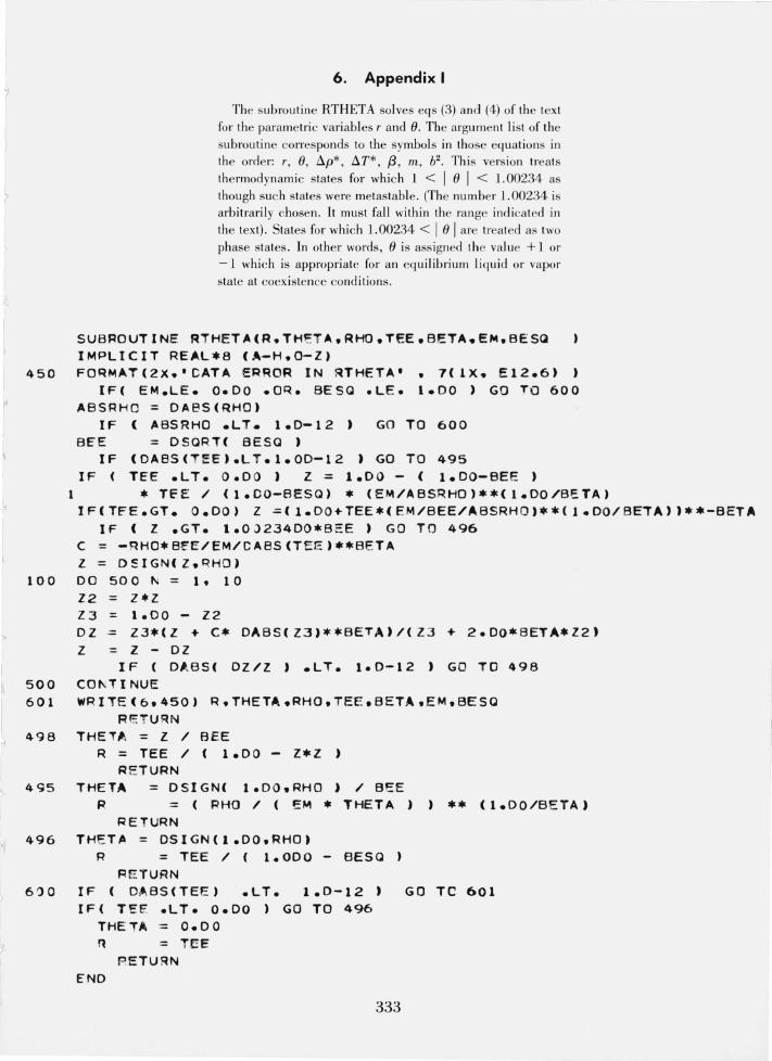
6. Appendix I

The subrout ine RTHETA solves eqs (3) and (4) of the text for the parametric variables r and 8. The argumen t list of the subrou tine corresponds to the symbols in those eq uations in th e order: r, 8, !1p*, !1T*, {3 , m , 62• Th is version treats thermodynamic states for which 1 < I 8 I < 1.00234 as though such states were metas table. (The nu mber 1.00234 is arbitraril y chosen. It must fall withi n the range ind ica ted in the text). Sta tes for which 1.00234 < I 8 I a re treated as two phase states . In other words, 8 is ass igned the value + 1 or - 1 which is appropriate for an equili briu m liquid or vapor state at coex istence cond itions.

SUBROUTINE RTHETA(R,TH~TA,RHO.TEE.BETA.EM.BESQ IMPLICIT REAL*8 (A-H.O-Z) FORMAT(2X.'CATA ERROR IN ~THETA' , 7(lX. E12.6)

IF( EM.LE. O.DO .OR. BESQ .LE. I.DO ) GO TO 600 ABSRHO = DAeS(RHO)

IF ( ABSRHO .LT. 1.0-12 ) GD TO 600 BEE = DSQRT( BESQ )

IF (DABS(TEE).LT.l.0D-12 ) GO TO 495 IF ( TEE .LT. O.DO) Z = 1.00 - ( I.DO-BEE

* TfE / (I.DO-BESa) * (EM/ABSRHO'**(l.DO/BETA) IF(TFE.GT. O.DO) Z =(l.DO+TEE*(EM/BEE/ABSRHO)**(l.DO/BETA')**-BETA

IF ( Z .GT. 1.OJ234DO*BEE ) GO TO 496 C = -~HO*BEE/EM/CABS(TEE )**B~TA Z = DSIGN(Z.RHO}

100 DO 50 0 N = 19 10

500 601

498

495

496

6')0

Z2 = Z*Z Z3 = 1.00 - 12 OZ Z

-=

Z3*(Z + C* DABS(Z3)**BETA'/(Z3 + 2.00*BETA*Z2) 1 - DZ

IF ( DABS( DZ/Z ) .LT. I.D-12 , GO TO 498 CONTINUE WRITE(6,~50) R.THETA.RHO,TEE,BETA.EM,BESQ

R ETU~N

THETA = Z / BEE R = TEE / ( 1.DO - z*z )

RETURN THETA = DSIGN( I.DO.RHO ) / BEE

R = ( RHO / ( ~M * THETA) ) ** (I.DO/BETA) RETURN

THETA = OSIGN(I.00.RHO) R = TEE / ( 1.0DO - BESQ

RETURN IF (D~ BS(TEE) .LT. I.D-12) IF( TE E .LT. 0.00 ) GO TO 496

THETA = O.DO R = TEE

RETURN END

333

GO TC 601

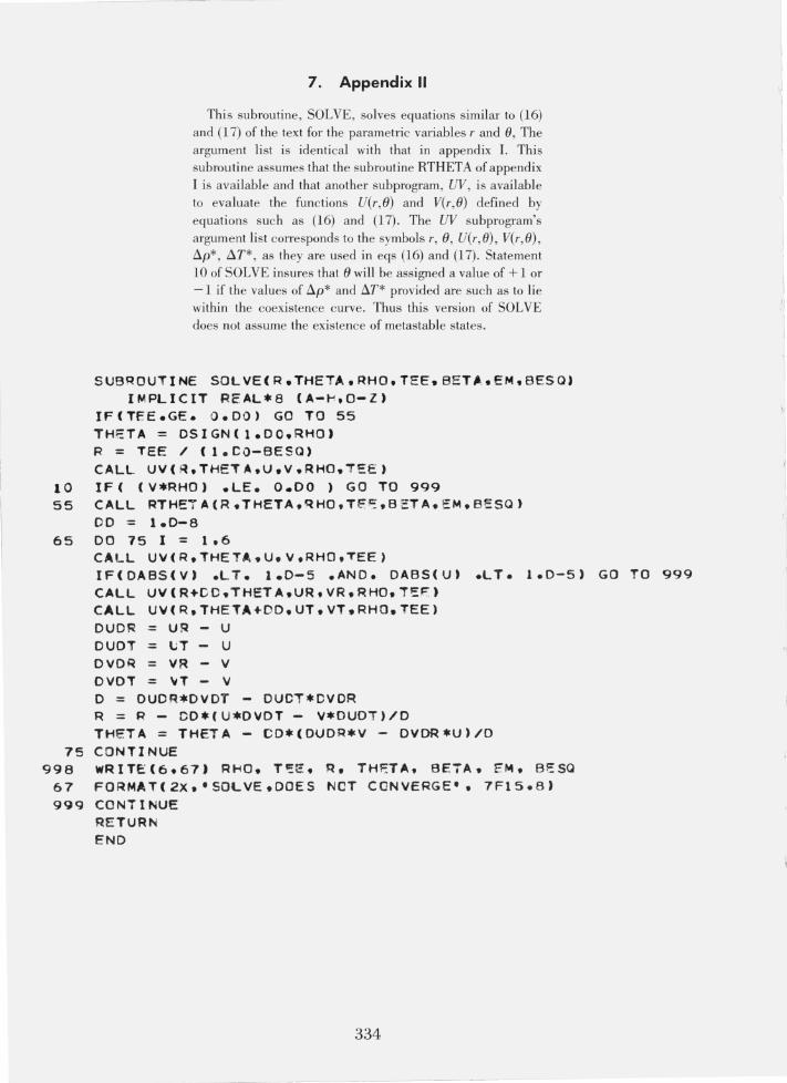
7. Appendix II

This subroutine, SOLVE, solves equations similar to (16) and (17) of the text for the parametric variables rand {}, The argument list is identical with that in appendix I. This subroutine ass umes that the subroutine RTHETA of appendix I is available and that another subprogram, UV, is available to evaluate the func tions U(r,{}) and V(r,{}) defined by equations such as (16) and (17). The UV subprogram's argument list corresponds to the symbols r, {}, U(r,{}), V(r,{}), !1p*, !1T*, as they are used in eqs (16) and (17). Statement 10 of SOLVE insures tha t {} will be assigned a value of + 1 or - 1 if the values of !1p* and !1T* provided are such as to lie within the coexistence curve. Thus this version of SOLVE does not assume the existence of metas table states.

SUBROUTINE SOLVE(R.THETA.RHO,TEE,BET •• EM,BESa) IMPLICIT REAL*8 (A-~.O-Z)

IF(TEE.GE. 0.00) GO TO 55 THETA = oSIGN(l.oO.RHO) R = TEE / (l.eO-SESa) CALL UV(R,THETA.U,v.RHO,TEE )

10 IF( (V*RHO) .LE. 0.00 ) GO TO 999 55 CALL RTHETA(R.THETA.qHO,T~~ .B ETA.EM.BESa)

00 = 1.0-8 65 DO 15 I = 1,6

CALL UV(R.THE TA,U.V.RHO.TEE) IF(DABS(V) .L T . 1.0-5 .AND. oABS(U' .LT. 1.0-5) GO TO 999 CALL UV(R+DC,THETA.UR,VR.RHO.iEF ) CALL UV(R.THETA+OD.UT.VT.RHO,TEE) DUDf< = U~ U DUo T == \;T U DVoR = VR V DVOT == \IT V o = OUD R*DVOT - OUCi*CVDR R = R - Co*CU*OVOT - V*oUoT)/o THE:T A = THET A - CO* (OUOR*V - OVDR *U) /0

75 CONTI NUE 998 wRITE(6.67) RHO, T~E. R. THF.TA. BEiA. EM. B~sa

67 FORMAT(2X,'SOLVE.DOES NeT CONVERGE'. 7 F15.8) 999 CONiINUE

RETURN END

334