Implementation of Intensity Model Approach to … of Intensity Model Approach to Constant Maturity...
42
1 Implementation of Intensity Model Approach to Constant Maturity Credit Default Swap Pricing Ohoe Kim Department of Mathematics, Towson University Towson, MD 21252
Transcript of Implementation of Intensity Model Approach to … of Intensity Model Approach to Constant Maturity...

1
Implementation of Intensity Model Approach to
Constant Maturity Credit Default Swap Pricing
Ohoe Kim
Department of Mathematics, Towson University
Towson, MD 21252

2
Abstract: Constant maturity credit default swaps (CMCDS) are useful as hedging tools. In
intensity model approach, the default time is defined as the first arrival time of the Poisson
process. From the market quotes of CDS forward rates and bonds, we are able to numerically
compute the default probabilities. Approximating CMCDS price depends largely on CDS
forward rates’ volatilities and their correlations. We implement the price algorithm based on
Brigo’s work (2006). Starting with current market data such as CDS forward rates and non-
defaultable bond prices, we describe steps involved to obtain the price CMCDS. We demonstrate
the impact of convexity on the CMCDS price structure.

3
Introduction
A Constant Maturity Credit Default Swap (CMCDS) is a combination of a Constant
Maturity Swap and Credit Default Swap. The valuation of a CMCDS is implemented in Excel
VBA and derives important quantities relating to CMCDS valuation based on the work of D.
Brigo[1]
1. Credit Default Swap (CDS)
A CDS contract insures protection against default. If a third company C (Reference
credit) defaults at the time cτ with a c bT Tτ< ≤ , then B (Protection Seller) pays to A (Protection
buyer) a certain cash amount LGD. In turn, A pays to B a rate R at time 1,a bT T+ L or until
default cτ .
2. Constant Maturity Credit Default Swap (CMCDS)
Consider a contract protecting in [ ,a bT T ] against default of a reference credit C.
If default occurs in [ ,a bT T ], a protection payment LGD is made from the protection seller B to the
protection buyer A at the first jT following the default time, called protection leg. A pays to B at
each jT before default a C+1 – long CMCDS rate i-1,i c 1R ( )iT+ −
B A
The value of the CMCDS to “B” is the value of the premium leg minus the value of the
protection leg.
GD a b c c
i-1,i c 1 i 1 c
protection L at default if T T R ( ) at T , , or until i a bT T T
τ ττ+ − +
→ < ≤ →← = ←K

4
3. Constant Maturity Swap (CMS)
A swap contract is when, on specified payment dates, party 1 agrees to pay the floating
LIBOR rate of a notional amount to party 2 and in return party 2 agrees to pay a fixed swap rate
to party 1 of the same notional amount. A constant maturity swap differs in that neither group
will be paying a fixed rate. In a constant maturity swap scenario, party 1 agrees to pay the
floating LIBOR rate on a notional amount to party 2 and party 2 will agree to pay a floating c-
period swap-rate (CMS rate) on the same notional amount to party 1. The CMS rate is not
constant and is calculated at the reset dates stated on the contract. The period of time ‘c’ used to
calculate the CMS rate will be stated in the contract. In essence both parties will be paying a
fluctuating rate. A CMS can be used to hedge against short term changes in interest rates.
4. CDS Payoff
Instead of considering the exact default timeτ , the protection payments LGD is postponed to
the first time iT following default and the premium payment R is paid at iT as long as the
default occurs after iT . Consequently the CDS payoff as seen from B can be expressed as
, 1{ } { }
1 1( ) : ( , ) 1 1 ( , )
a b i i i
b b
PRCDS i i T T T i GDi a i a
t D t T R D t T Lτ τα−≥ < ≤
= + = +
Π = −∑ ∑
where iα is the year fraction between iT and 1iT − and ( , )iD t T is a stochastic discount factor at
time t for maturity iT .
5. CDS Value at time t
The CDS price with respect to the risk neutral valuation can be written as
5
,
,
,
{ }
( , , ) { ( ) | }
1[ ( ) | ]
Pr( | )
a b
a b
a b GD PRCDS t
tPRCDS t
t
PRCDS t R L E t G
E t Ft F
τ
τ>
= Π
= Π>
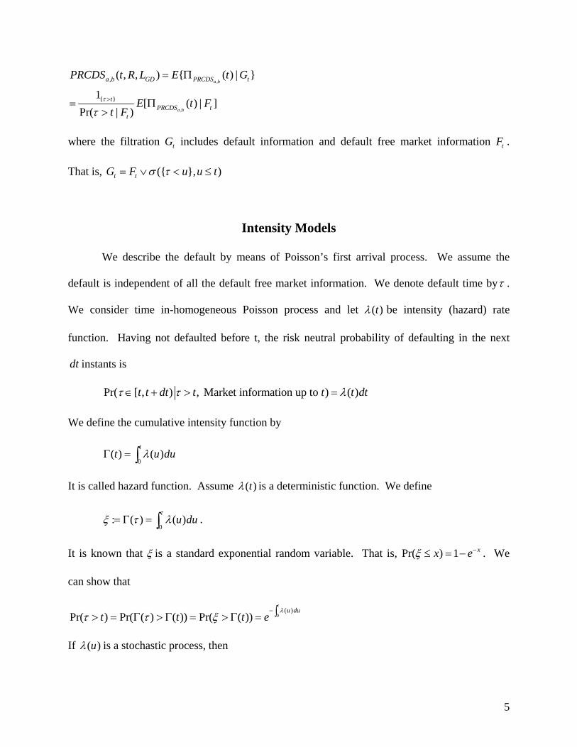
where the filtration tG includes default information and default free market information tF .
That is, ({ }, )t tG F u u tσ τ= ∨ < ≤
Intensity Models
We describe the default by means of Poisson’s first arrival process. We assume the
default is independent of all the default free market information. We denote default time byτ .
We consider time in-homogeneous Poisson process and let ( )tλ be intensity (hazard) rate
function. Having not defaulted before t, the risk neutral probability of defaulting in the next
dt instants is
Pr( [ , ) , Market information up to ) ( )t t dt t t t dtτ τ λ∈ + > =
We define the cumulative intensity function by
0( ) ( )
tt u duλΓ = ∫
It is called hazard function. Assume ( )tλ is a deterministic function. We define
0: ( ) ( )u du
τξ τ λ= Γ = ∫ .
It is known that ξ is a standard exponential random variable. That is, Pr( ) 1 xx eξ −≤ = − . We
can show that
0( )
Pr( ) Pr( ( ) ( )) Pr( ( ))t
u dut t t e
λτ τ ξ
−∫> = Γ > Γ = > Γ =
If ( )uλ is a stochastic process, then

6
0( )
Pr( ) Pr( ( ) ( )) Pr( ( )) [ ]t
u dut t t E e
λτ τ ξ
−∫> = Γ > Γ = > Γ =
( ) ( )( ) ( )Prt
su dus ts t e e e
λτ −Γ −Γ ∫< ≤ = − ≈
The defaultable bond price ( , )P t T is defined as:
( ( ) ( ))
{ } { }1 ( , ) [ ( , )1 ] [ ]T
tr u u du
t T tP t T E D t T G E eλ
τ τ
− +
> >∫= =
Thus, the survival probability looks like the price of a zero coupon bond in an interest rate model
with short rate r replaced by ( )tλ and ( )tλ is interpreted as instantaneous credit spread. In
particular,
0( ( ) ( ))
{ }(0, ) [ (0, )1 ] [ ]T
r u u du
T tP T E D T G E eλ
τ
− +
>∫= =
The Filtration Switching Formula
It can be shown that the following switching formula is valid:
{ }{ } { }
1[1 ] [1 ]
{ }t
T t T tt
E Payoff G E Payoff FQ t F
ττ ττ
>> >=
>
where Q represents probability.
The proof of this result is in the reference [1]. Switching from tG to tF is useful because most
times it is easy to compute the tF conditional expectation.
CDS Forward Rates
The CDS forward rates can be defined as that rate R that makes the CDS value equal to
zero at time t. That is, ,, ( , , ) { ( ) | } 0
a ba b GD PRCDS tCDS t R L E t G= Π = . where Π represents CDS
payoff at time t .

7
A defaultable zero coupon bond (DZCB), ( , )P t T is defined as
{ } { }1 ( , ) : [ ( , )1 | ]t T tP t T E D t T Gτ τ> >=
Using the filtration switching formula, the following expression can be obtained
{ }[ ( , )1 | ] ( | ) ( , )T t tE D t T F Q t F P t Tτ τ> = >
,
,
,
{ }
( , , ) [ ( ) ]
1[ ( ) ]
Pr( )
a b
a b
a b GD PRCDS t
tPRCDS t
t
CDS t R L E t G
E t Ft F
τ
τ>
= Π
= Π>
1
{ }{ } { }
1 1
1( , ) 1 ( , )1
( ) i i i
b bt
i i T t GD i T T ti a i at
E D t T R F L E D t T FQ t F
ττ τα
τ −
>> < ≤
= + = +
⎧ ⎫⎡ ⎤ ⎡ ⎤= −⎨ ⎬⎣ ⎦ ⎣ ⎦> ⎩ ⎭∑ ∑
( )1
{ }{ }
1 1
1( , ) ( , )1
( ) i i
b bt
i t i GD i T T ti a i at
RQ t F P t T L E D t T FQ t F
ττα τ
τ −
>< ≤
= + = +
⎧ ⎫⎡ ⎤= > −⎨ ⎬⎣ ⎦> ⎩ ⎭∑ ∑
Hence, we have this expression,
1 1{ } { }1 1
,
{ }1 1
[ ( , )1 | ] [ ( , )1 | ]( )
[ ( , )1 ] Pr( ) ( , )
i i i i
i
b b
GD i T T t GD i T T tPR i a i aa b b b
i i T t i t ii a i a
L E D t T F L E D t T FR t
E D t T F t F P t T
τ τ
τα α τ
− −< < < <= + = +
>= + = +
= =>
∑ ∑
∑ ∑
CDS Options
Consider the option for a protection buyer to enter a CDS at a future time 0aT > , a bT T< ,
paying a fixed premium rate K at times 1,...,a bT T+ or in exchange for a protection payment GDL
until default happens in [ , ]a bT T . This option expires at aT . The discounted CDS option payoff at
time t is:
, , , ,
,
( ; ) ( , ) ( , ( ), ) ( , , )
( , ) ( , , )
a bcallPRCDS a a b a a b a GD a b a GD
a a b a GD
t K D t T CDS T R T L CDS T K L
D t T CDS T K L
+
+
⎡ ⎤Π = −⎣ ⎦
⎡ ⎤= −⎣ ⎦

8
which can be also written:
,
{ },
1
1( ; ) ( , ) ( ) ( , ) ( ( ) )
( )a
a b
a
bT
callPRCDS a i a Ta a i a b ai aa T
t K D t T Q T F P T T R T KQ T F
τ α ττ
> +
= +
⎡ ⎤Π = > −⎢ ⎥> ⎣ ⎦∑
Thus, we obtain the market formula for CDS option:
{ },,
{ } , ,
{ } , , 1 2
( , , ) ( , ; )
1 ( , ) ( )( ( ) )
1 ( ) ( ) ( ( )) ( ( ))
a b
a
a b GD CallCDS GD t
T a a b a a b a t
t a b a b
CallCDS t K L E t K L G
E D t T C T R T K G
C t R t N d t KN d t
τ
τ
+>
>
⎡ ⎤= Π⎣ ⎦
= −
⎡ ⎤= −⎣ ⎦
where
2, ,
1,2,
ln( ( ) ( )( ) )
2a b a a b
a b a
R t T tKd
T t
σ
σ
−±
=−
One period CDS forward rate ( )jR t
, ( )a bR t can be expressed as a linear combination of one period CDS forward rates ( )jR t
as the swap rate, , ( )a bS t is expressed as a linear combination of forward rates
1( ) ( , , )j j jF t F t T T−= . The one period CDS rates is defined as
1{ }
1,
( , ) 1( ) ( ) :
( ) ( , )j jGD j T T t
j j jj t j
L E D t T FR t R t
Q t F P t Tτ
α τ− < <
−
⎡ ⎤⎣ ⎦= =
>
Let ( , )ip t T be a zero-coupon bond, and 1( ) ( , , )i i iF t F t T T−= be a forward rate maturing at iT . The
swap rate is defined as:
1,
1
( , ) ( )( )
( , )
b
i i ii a
a b b
i ii a
P t T F tS t
P t T
α
α
= +
= +
=∑
∑
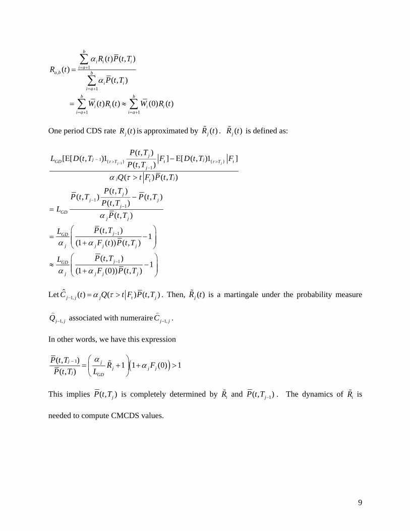
Likewise, we define the credit default swap rate as:
9
1,
1
1 1
( ) ( , )( )
( , )
( ) ( ) (0) ( )
b
i i ii a
a b b
i ii a
b b
i i i ii a i a
R t P t TR t
P t T
W t R t W R t
α
α
= +
= +
= + = +
=
= ≈
∑
∑
∑ ∑
One period CDS rate ( )jR t is approximated by ( )jR t% . ( )jR t% is defined as:
11 { } { }
1
11
1
1
( , )[ [ ( , )1 ] [ ( , )1 ]
( , )( ) ( , )
( , )( , ) ( , )
( , )( , )
( , )1
(1 ( )) ( , )
( , )(1 (0)) ( ,
j j
jj jGD T t T t
j
j jt
jj j
jGD
j j
jGD
j j j j
jGD
j j j
P t TL D t T F D t T F
P t TQ t F P t T
P t TP t T P t T
P t TL
P t T
P t TLF t P t T
P t TLF P t T
τ τ
α τ
α
α α
α α
−− > >
−
−−
−
−
Ε − Ε
>
−=
⎛ ⎞= −⎜ ⎟⎜ ⎟+⎝ ⎠
≈+
1)j
⎛ ⎞−⎜ ⎟⎜ ⎟
⎝ ⎠
Let 1,ˆ ( ) ( ) ( , )j j j t jC t Q t F P t Tα τ− = > . Then, ( )jR t% is a martingale under the probability measure
1,j jQ −
) associated with numeraire 1,j jC −
).
In other words, we have this expression
( )1( , ) 1 1 (0) 1( , )
j jj j j
j GD
P t T R FP t T L
αα− ⎛ ⎞
= + + >⎜ ⎟⎝ ⎠
%
This implies ( , )jP t T is completely determined by iR% and 1( , )jP t T − . The dynamics of iR% is
needed to compute CMCDS values.

10
One period CDS rate approximation and dynamics
First, iR% is a Martingale under ˆ iQ measure as long as iR% remains positive.
ii i i idR R dZσ=% % under ˆ iQ measure
Second, we need to change a probability measure from ˆ iQ to ˆ jQ for all i j≥ . The following
result is obtained and the proof is in the reference [1].
ii i i idR R dZσ=% % under ˆ iQ measure
,1
j
jh hi i i h i
GDh ih
h
RR dt dZLR
σσ ρ
α= +
⎛ ⎞⎜ ⎟⎜ ⎟= +⎜ ⎟+⎜ ⎟⎝ ⎠
∑%
%%
[ ( ) ]j ji i i iR R dt Zμ σ= +% % under ˆ jQ measure
where ,i hρ is a correlation of iR% and hR%
Hence, Monte Carlo simulation is possible given (0)R% , the volatilities and correlations.
Furthermore, the expected value of 1( )i jR T −% under ˆ jQ measure is computed.
We assume the volatility iσ is piecewise constant.
Let ,1
(0)
(0)
ij h h
i i h iGDh j
hh
RLR
σμ ρ σ
α= +
⎛ ⎞⎜ ⎟⎜ ⎟=⎜ ⎟+⎜ ⎟⎝ ⎠
∑%
%%
. Then we have
{ }11,1 10
1
(0)ˆ ( ) (0)exp ( (0)) (0)exp(0)
jiTj j j h h
i j i i i j i ihGDh j
hh
RE R T R R du R T LR
σμ σ ρ
α
−−− −
= +
⎡ ⎤⎛ ⎞⎢ ⎥⎜ ⎟⎢ ⎥⎜ ⎟⎡ ⎤ = ≈⎣ ⎦ ⎢ ⎥⎜ ⎟+⎜ ⎟⎢ ⎥⎝ ⎠⎣ ⎦
∑∫%
% % % %%%

11
Calibration Technique
We use the intensity models to obtain implied default probabilities from market quotes.
We assume the intensity rate function ( )tγ to be deterministic and piecewise function.
( ) 1
1 ( ) 1 ( )01
( ) ( ) ( ) ( )tt
i i i t ti
t s ds T T t Tβ
β βγ γ γ−
+ −=
Γ = = − + −∑∫
101
: ( ) ( )jjT
j i i ii
s ds T Tγ γ−=
Γ = = −∑∫
We have the following expression for the Protection leg at time 0:
1
1
1
1
{ } 01
{ }01
1
01
11
[ (0, )1 | ]
[ (0, )1 ]Pr( [ , ))
[ (0, )]Pr( [ , ))
(0, ) ( )exp( ( ) )
exp( (
i i
i i
i
i
i
i
b
GD i T Ti a
b
GD i T Ti a
b T
GD iTi a
b T u
GD iTi a
b
GD i i ii a
L E D T F
L E D T u u du
L E D T u u du
L P T u s ds du
L
τ
τ τ
τ
γ γ
γ γ
−
−
−
−
< <= +
∞
< <= +
= +
= +
−= +
⋅
= ∈ +
= ∈ +
= −
= −Γ −
∑
∑∫
∑ ∫
∑ ∫ ∫
∑1
1)) (0, )i
i
T
i iTu T P T du
−−−∫
We also have the expression for the Premium leg at time 0
{ }1
{ }1
1
1
[ (0, ) 1 ]
[ (0, )] [1 ]
(0, ) Pr( )
(0, ) Pr( )
i
i
b
i i Ti a
b
i i Ti a
b
i i ii a
b
i i ii a
E D T R
E D T RE
P T R T
R P T T
τ
τ
α
α
α τ
α τ
≥= +
≥= +
= +
= +
=
= ≥
= ≥
∑
∑
∑
∑
It can be shown that

12
1
,
( ) ( ) ( ) ( )
1 1
( , , ; ( ))
( , ) ( , ) ( )]ii
i
a b GD
b b Tt T u ti i GD i uT
i a i a
CDS t R L
P t T R e L P t T d eα−
Γ −Γ −Γ −Γ
= + = +
Γ ⋅
= +∑ ∑ ∫
In particular, under the piecewise assumption on 1( ) , [ , ]i i i it T Tγ γ γ −= ∈ , we have,
1
,
( ( ) ( ))1 1
1 1
( , , ; ( ))
( , ) exp( ( )) (0, )ii
i
a b GD
b b TT ti i GD i i i i iT
i a i a
CDS t R L
P t T R e L u T P T duα γ γ−
− Γ −Γ− −
= + = +
Γ ⋅
= − −Γ − −∑ ∑ ∫
Here we use the discrete form of the CDS value at time 0 to implement in computation scheme to
estimate the piecewise constant intensity.
, ,
1
1 1 11
1 1
(0, , )
(0, ) exp( ( ))
(0, ) ( ) exp( ( ))( )
(0, ) exp( ( )) (0, ) exp( )
a b GD
b
i i ii a
b
GD i i i i i i i ii ab b
i i i GD i i i ii a i a
CDS R L
R P T T
L P T T T T T T
R P T T L P T
α
γ γ
α γ α
= +
− − −= +
= + = +
Γ
= −Γ
− −Γ − − −
= −Γ − −Γ
∑
∑
∑ ∑
where 1i i iT Tα −= − and 1( ) , [ , ]i i i it T Tγ γ γ −= ∈
In the market 0aT = and we have R quotes for 1,2,3,....,10bT = years, by setting iT quarterly, we
can solve the
0,1 0,1 1 2 3 4 1
0,2 0,2 1 5 6 7 8 2
(0, , ; ; ) 0
(0, , ; ; ; ) 0
MGD
MGD
CDS R L
CDS R L
γ γ γ γ γ
γ γ γ γ γ γ
= = = =
= = = =
by Matlab Software. See the code in the Appendix.
Numerical Example
At this point, we present some numerical examples, based on IBM Company CDS data
on 28th, October, 2008.

13
Recovery Rate= 40%
Maturity Tb(yr) Maturity (date) R(0,Tb)
0.5 2009‐4‐28 39.1 1 2009‐10‐28 47.327
2 2010‐10‐28 54.669 3 2011‐10‐28 63.894
4 2012‐10‐28 72.652 5 2013‐10‐28 77.16
7 2015‐10‐28 77.472 10 2018‐10‐28 79.439
Table 1 Maturity dates and corresponding CDS quotes in bps for 0T =28th, October, 2008.
Date Intensity Survival Probability
2009‐4‐28 0.0065167 99.675% 2009‐10‐28 0.009276 99.213%
2010‐10‐28 0.010365 98.190% 2011‐10‐28 0.013868 96.838%
2012‐10‐28 0.016849 95.220% 2013‐10‐28 0.016254 93.685%
2015‐10‐28 0.013067 91.268% 2018‐10‐28 0.014322 87.430% Table 2 Calibration with piecewise linear intensity on 28th, October, 2008.

14
Oct-08 Oct-09 Oct-10 Oct-11 Oct-12 Oct-13 Oct-15 Oct-180.6%
0.8%
1%
1.2%
1.4%
1.6%
1.8%
2%Piecewise Constant Intensity
Figure 1 Piecewise constant intensity γ calibrated on CDS quotes on October 28th 2008.
Oct-08 Oct-09 Oct-10 Oct-11 Oct-12 Oct-13 Oct-14 Oct-15 Oct-16 Oct-17 Oct-18 86%
88%
90%
92%
94%
96%
98%
100%Survival Probability
Figure 2 Survival Probability exp( )−Γ resulting from calibration on CDS quotes on October
28th, 2009
15
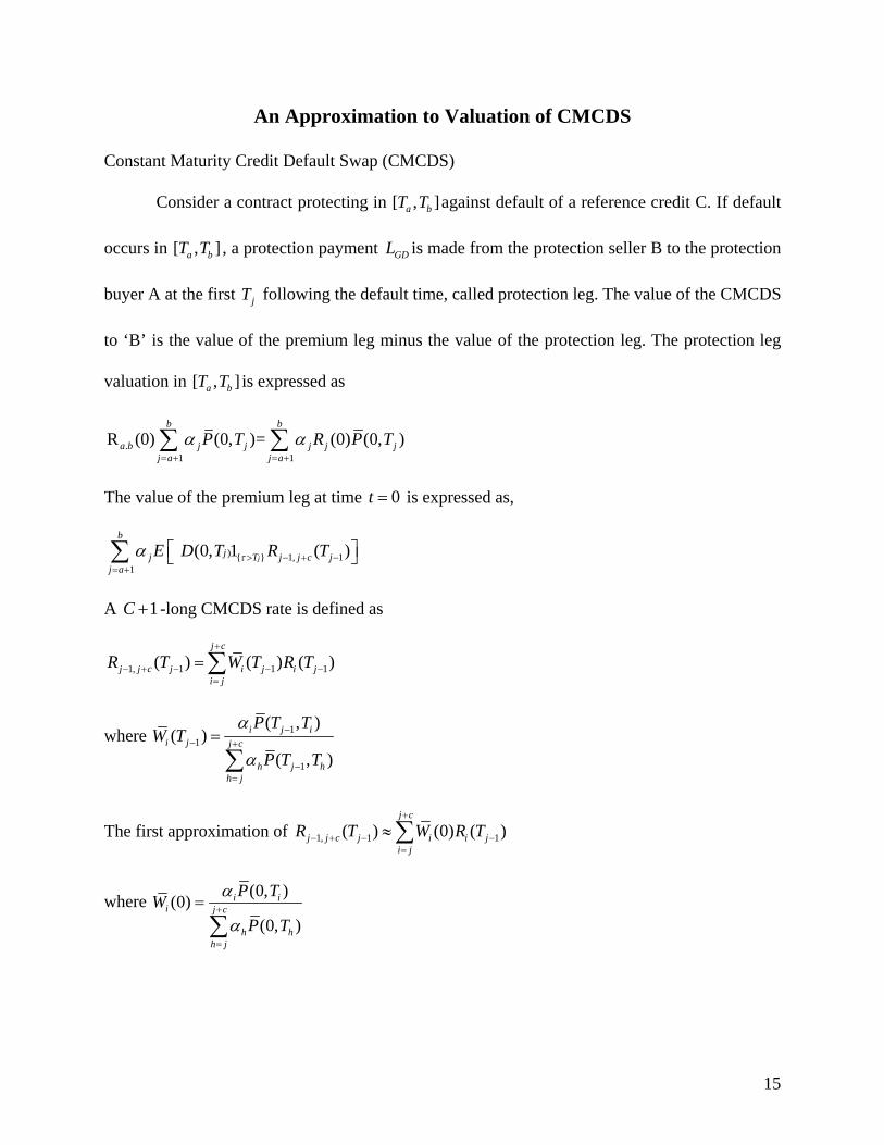
An Approximation to Valuation of CMCDS
Constant Maturity Credit Default Swap (CMCDS)
Consider a contract protecting in [ , ]a bT T against default of a reference credit C. If default
occurs in [ , ]a bT T , a protection payment GDL is made from the protection seller B to the protection
buyer A at the first jT following the default time, called protection leg. The value of the CMCDS
to ‘B’ is the value of the premium leg minus the value of the protection leg. The protection leg
valuation in [ , ]a bT T is expressed as
.1 1
R (0) (0, )= (0) (0, )b b
a b j j j j jj a j a
P T R P Tα α= + = +∑ ∑
The value of the premium leg at time 0t = is expressed as,
) { } 1, 11
(0, 1 ( )j
b
jj T j j c jj a
E D T R Tτα > − + −= +
⎡ ⎤⎣ ⎦∑
A 1C + -long CMCDS rate is defined as
1, 1 1 1( ) ( ) ( )j c
j j c j i j i ji j
R T W T R T+
− + − − −=
=∑
where 11
1
( , )( )
( , )
i j ii j j c
h j hh j
P T TW T
P T T
α
α
−− +
−=
=
∑
The first approximation of 1, 1 1( ) (0) ( )j c
j j c j i i ji j
R T W R T+
− + − −=
≈∑
where (0, )(0)(0, )
i ii j c
h hh j
P TWP T
α
α+
=
=
∑

16
) { } 1, 11
) { } 1, 11
1,1, 1
1
1,1
1
(0, 1 ( )
(0) (0, 1 ( )
ˆ ˆ(0) (0) ( )
ˆ(0) (0, ) ( )
j
ji
i
i
b
jj T j j c jj a
j cbj
jj T j j c jj a i j
j cbj j j
j j j i jj a i j
j cbj j j
j j i jj a i j
E D T R T
W E D T R T
W C E R T
W P T E R T
τ
τ
α
α
α
α
> − + −= +
+
> − + −= + =
+−
− −= + =
+−
−= + =
⎡ ⎤⎣ ⎦
⎡ ⎤≅ ⎣ ⎦
⎡ ⎤= ⎣ ⎦
⎡=
∑
∑ ∑
∑ ∑
∑ ∑ ⎤⎣ ⎦
We need to compute 1,1
ˆ ( )j ji jE R T−
−⎡ ⎤⎣ ⎦ . We approximate the expectation by 1,1
ˆ ( )j ji jE R T−
−⎡ ⎤⎣ ⎦% .
{ }1
1
1,1 0
, 01
ˆ ( ) (0)exp ( (0))
(0)(0)exp ( ) ( )(0)
j
j
Tj j ji j i i
i TKi i k i k
GDk jK
K
E R T R R du
RR u u duLR
μ
ρ σ σ
α
−
−
−−
= +
⎡ ⎤ ≅⎣ ⎦
⎧ ⎫⎪ ⎪⎪ ⎪= ⎨ ⎬⎪ ⎪+⎪ ⎪⎩ ⎭
∫
∑ ∫
% % %%
%%
%
Assume iσ is piecewise constant
{ }11,1 0
1 ,1
ˆ ( ) (0) exp ( (0))
(0)(0)exp(0)
jTj j ji j i i
ik k
i j i i kGDk j
Kk
E R T R R du
RR T LR
μ
σσ ρ
α
−−−
−= +
⎡ ⎤ ≅⎣ ⎦
⎧ ⎫⎛ ⎞⎪ ⎪⎜ ⎟⎪ ⎪⎜ ⎟≈ ⎨ ⎬
⎜ ⎟⎪ ⎪+⎜ ⎟⎪ ⎪⎝ ⎠⎩ ⎭
∫
∑
% % %%
%%
%
The value of CMCDS at 0t =
, ,1
11
(0, )(0, ) (0, ) (0, )
(0) (0)exp (0)(0)
j cbi i
GDCMa b c j j j cj a i j h hh j
ik k
i j i ik jGDk j
kk
P TCDS L P TP T
RR T RLR
ααα
σσ ρ
α
+
+= + =
=
−= +
⎧⎪= ⎨⎪⎩
⎫⎡ ⎤⎛ ⎞⎪⎢ ⎥⎜ ⎟ ⎪⎢ ⎥⎜ ⎟ − ⎬
⎢ ⎥⎜ ⎟ ⎪+⎜ ⎟⎢ ⎥ ⎪⎝ ⎠⎣ ⎦ ⎭
∑ ∑∑
∑%
%%
The detailed proof of this result is in the reference [1].

17
Important Quantities for Comparisons
The following quantities are worthy of consideration for comparison. We define iL
as 1,
0,
(0)(0)
i i c
b
RR− + . This measures how the CMCDS differs from a standard CDS at the premium rate
at each period. We define iM as follows,
{ } 1, 1
1,1
(0, )1 ( )
ˆ(0) (0, )* ( )
ii T i i c i
i ci i
j i j ij i
A E D T R T
W P T E R T
τ > − + −
+−
−=
⎡ ⎤= ⎣ ⎦
⎡ ⎤= ⎣ ⎦∑ %
1,1 1 ,
1
(0)ˆ ( ) (0)exp(0)
ji i k k
j i j i j j kGDk i
Kk
RE R T R T LR
σσ ρ
α
−− −
= +
⎧ ⎫⎛ ⎞⎪ ⎪⎜ ⎟⎪ ⎪⎜ ⎟⎡ ⎤ ≈ ⎨ ⎬⎣ ⎦ ⎜ ⎟⎪ ⎪+⎜ ⎟⎪ ⎪⎝ ⎠⎩ ⎭
∑%
% %
%
0,(0, ) (0)ii b
AMP T R
=
The quantity iM is the same as iL except taking into consideration the expression of the random
values and correlations. We define iN as follows,
1,0 { } 1, 1
1,
ˆ [ (0, )1 ( )](0, ) (0)
i
i ii T i i c i
ii i i c
E D T R TN
P T Rτ
−> − + −
− +
=
This is a measure of the impact of the convexity at each period in the premium leg.
We define iX as follows,
0,1
1,1
(0, ) (0)" "" " (0, ) (0)
ij j ij
i ij j j j cj
P T Rpremium leg CDSXpremium leg CMCDS P T R
α
α=
− +=
= =∑∑

18
We define iY as follows,
0,1
1,0 { } 1, 11
" "Y" "
(0, ) (0)ˆ [ (0, )1 ( )
j
i
ij j ij
i j jj j T j j c jj
premium leg CDSpremium leg CMCDS with convexity
P T R
E D T R Tτ
α
α=
−> − + −=
=
=∑
∑
In this case the convexity due to correlation and volatilities are taken into consideration.
We make a note of the difference between two quantities:
0,1
(0, ) (0)N
j j Nj
premiumlegCDS P T Rα=
=∑
{ } 1, 1 11
(0, )1 ( )j
N
j j T j j c jj
premiumlegCMCDS E D T R Tτα > − − + −=
⎡ ⎤= ⎣ ⎦∑
Numerical Implementation and Procedure
This will be implemented in Excel VBA. The CMCDS value at 0t = is based on
, ,1
11
(0, )(0, ) (0, ) (0, )
(0) (0)exp (0)(0)
j cbi i
GDCMa b c j j j cj a i j h hh j
ik k
i j i ik jGDk j
kK
P TCDS L P TP T
RR T RLR
ααα
σσ ρ
α
+
+= + =
=
−= +
⎧⎪= ⎨⎪⎩
⎫⎡ ⎤⎛ ⎞⎪⎢ ⎥⎜ ⎟ ⎪⎢ ⎥⎜ ⎟ − ⎬
⎢ ⎥⎜ ⎟ ⎪+⎜ ⎟⎢ ⎥ ⎪⎝ ⎠⎣ ⎦ ⎭
∑ ∑∑
∑%
%%
(1)

19
The list of inputs is as follows,
Inputs
ijρ
iσ
i(0,T )p
GDL
a,b,c iT
1i i iT Tα −= −
0, (0)bR
ijρ represents the instantaneous correlation between and i jR R , and iσ represents the volatility
of ( )iR t . i(0,T )p and the market value 0, (0)bR are available in the appendix.
The list of intermediate inputs is as follows,
Intermediate Inputs
(t)λ
Q( )iTτ >
(0, ) (0, )*Q( )i i ip T p T Tτ= >
We use the intensity model to obtain implied default probability from market quotes under the
assumption that there is independence between interest rates and the default time. We need a
calibration process to extract implied hazard rates and iQ( T )τ > . We have the following
equation,
1,
1
1 1
( ) ( , )( )
( , )
( ) ( ) (0) ( )
b
i iii a
a b biii a
b b
i i i ii a i a
R t P t TR t
P t T
W t R t W R t
α
α= +
= +
= + = +
=
= ≈
∑∑
∑ ∑
(2)
Then, ( )iR t is approximated by ( )iR t% .

20
We make use of the expression,
1, 1 1 1( ) ( ) ( )j c
j j c j i j i ji j
R T W T R T+
− + − − −=
=∑
where 11
1
( , )( )
( , )
i j ii j j c
h j hh j
P T TW T
P T T
α
α
−− +
−=
=
∑
1, 1 1( ) (0) ( )j c
j j c j i i ji j
R T W R T+
− + − −=
≈∑ (3)
where (0, )(0)(0, )
i ii j c
h hh j
P TWP T
α
α+
=
=
∑
(0)KR% is an approximation of (0)KR
11
(0, )(0, ) (0, )(0, )(0)
(0, )
KK K
KGDKK K
P TP T P TP TR L
P Tα
−−
−=% (4)
The price of the premium leg at 0t =
) { } 1, 11
1,1
1
(0, 1 ( )
ˆ(0) (0, ) ( )
j
i
b
jj T j j c jj a
j cbj j j
j j i jj a i j
E D T R T
W P T E R T
τα
α
> − + −= +
+−
−= + =
⎡ ⎤⎣ ⎦
⎡ ⎤= ⎣ ⎦
∑
∑ ∑ (5)
{ }11,1 0
1 ,1
ˆ ( ) (0) exp ( (0))
(0) (0)exp(0)
jTj j ji j i i
ik k
i j i j kGDk j
Kk
E R T R R du
RR T LR
μ
σσ ρ
α
−−−
−= +
⎡ ⎤ ≅⎣ ⎦
⎧ ⎫⎛ ⎞⎪ ⎪⎜ ⎟⎪ ⎪⎜ ⎟≈ ⎨ ⎬
⎜ ⎟⎪ ⎪+⎜ ⎟⎪ ⎪⎝ ⎠⎩ ⎭
∫
∑
% % %%
%%
%
(6)
21
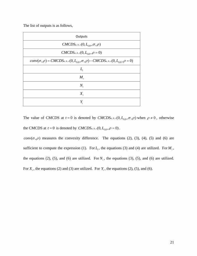
The list of outputs is as follows,
Outputs
, , (0, , , )a b c GDCMCDS L σ ρ
, , (0, , 0)a b c GDCMCDS L ρ =
, , , ,( , ) (0, , , ) (0, , 0)a b c a b cGD GDconv CMCDS L CMCDS Lσ ρ σ ρ ρ= − =
iL
iM
iN
iX
iY
The value of CMCDS at 0t = is denoted by , , (0, , , )a b c GDCMCDS L σ ρ when 0ρ ≠ , otherwise
the CMCDS at 0t = is denoted by , , (0, , 0)a b c GDCMCDS L ρ = .
( , )conv σ ρ measures the convexity difference. The equations (2), (3), (4), (5) and (6) are
sufficient to compute the expression (1). For iL , the equations (3) and (4) are utilized. For iM ,
the equations (2), (5), and (6) are utilized. For iN , the equations (3), (5), and (6) are utilized.
For iX , the equations (2) and (3) are utilized. For iY , the equations (2), (5), and (6).

22
Numerical Samples and Results:
• Ford Company on July 1st, 2008 Inputs: LGD=0.6 Maturity Tb(yr) Maturity (date) R(0,Tb) 0.5 2009‐1‐1 700 1 2009‐7‐1 1188.89 2 2010‐7‐1 1664.141 3 2011‐7‐1 1936.845 4 2012‐7‐1 2010.546 5 2013‐7‐1 2043.658 7 2015‐7‐1 1980.742 10 2018‐7‐1 1922.815 Table 3 Maturity dates and corresponding CDS quotes in bps for 0T = July 1st,2008
a=0 b=20 c=10 assume constant volatility for all R(0) 0.4σ = assume constant correlation ρ 0.9ρ = Table 4 Constant volatility and correlation
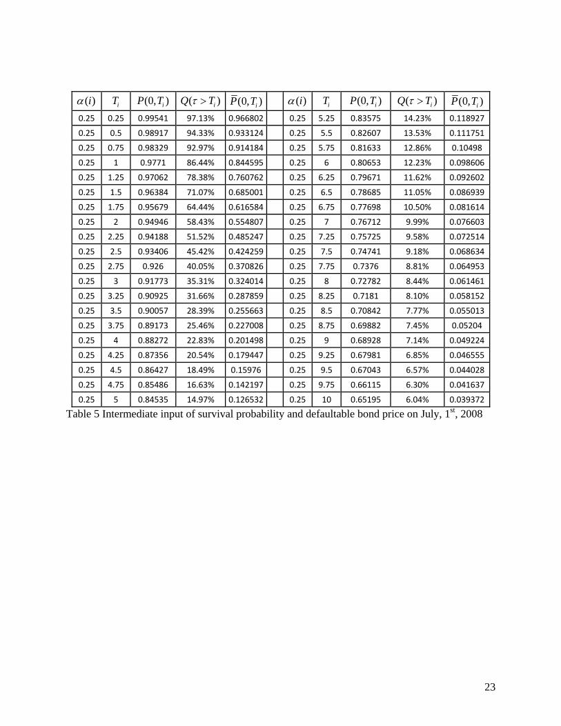
23
( )iα iT (0, )iP T ( )iQ Tτ > (0, )iP T ( )iα iT (0, )iP T ( )iQ Tτ > (0, )iP T0.25 0.25 0.99541 97.13% 0.966802 0.25 5.25 0.83575 14.23% 0.118927
0.25 0.5 0.98917 94.33% 0.933124 0.25 5.5 0.82607 13.53% 0.111751
0.25 0.75 0.98329 92.97% 0.914184 0.25 5.75 0.81633 12.86% 0.10498
0.25 1 0.9771 86.44% 0.844595 0.25 6 0.80653 12.23% 0.098606
0.25 1.25 0.97062 78.38% 0.760762 0.25 6.25 0.79671 11.62% 0.092602
0.25 1.5 0.96384 71.07% 0.685001 0.25 6.5 0.78685 11.05% 0.086939
0.25 1.75 0.95679 64.44% 0.616584 0.25 6.75 0.77698 10.50% 0.081614
0.25 2 0.94946 58.43% 0.554807 0.25 7 0.76712 9.99% 0.076603
0.25 2.25 0.94188 51.52% 0.485247 0.25 7.25 0.75725 9.58% 0.072514
0.25 2.5 0.93406 45.42% 0.424259 0.25 7.5 0.74741 9.18% 0.068634
0.25 2.75 0.926 40.05% 0.370826 0.25 7.75 0.7376 8.81% 0.064953
0.25 3 0.91773 35.31% 0.324014 0.25 8 0.72782 8.44% 0.061461
0.25 3.25 0.90925 31.66% 0.287859 0.25 8.25 0.7181 8.10% 0.058152
0.25 3.5 0.90057 28.39% 0.255663 0.25 8.5 0.70842 7.77% 0.055013
0.25 3.75 0.89173 25.46% 0.227008 0.25 8.75 0.69882 7.45% 0.05204
0.25 4 0.88272 22.83% 0.201498 0.25 9 0.68928 7.14% 0.049224
0.25 4.25 0.87356 20.54% 0.179447 0.25 9.25 0.67981 6.85% 0.046555
0.25 4.5 0.86427 18.49% 0.15976 0.25 9.5 0.67043 6.57% 0.044028
0.25 4.75 0.85486 16.63% 0.142197 0.25 9.75 0.66115 6.30% 0.041637
0.25 5 0.84535 14.97% 0.126532 0.25 10 0.65195 6.04% 0.039372
Table 5 Intermediate input of survival probability and defaultable bond price on July, 1st, 2008
24
July-08 July-09 July-10 July-11 July-12 July-13 July-15 July-1810%
15%
20%
25%
30%
35%
40%
45%
50%
55%
60%Piecewise Constant Intensity
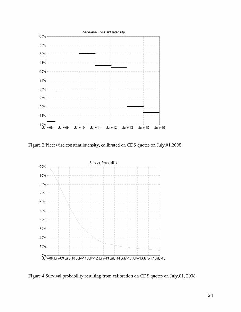
Figure 3 Piecewise constant intensity, calibrated on CDS quotes on July,01,2008
July-08July-09 July-10 July-11July-12 July-13 July-14 July-15 July-16 July-17 July-18 0%
10%
20%
30%
40%
50%
60%
70%
80%
90%
100%Survival Probability
Figure 4 Survival probability resulting from calibration on CDS quotes on July,01, 2008

25
Outputs:
Case 1: Constant volatilities
CMCDS(0, LGD, σ, ρ) ρ 0.7 0.8 0.9 0.99 σ 0.1 0.547515 0.547917 0.548319 0.548682 0.2 0.556096 0.557766 0.559448 0.560971 0.4 0.593735 0.601566 0.609628 0.61709 0.6 0.670855 0.694274 0.719441 0.743726
CMCDS(0, LGD, ρ=0) 0.544722 Table 6 Value of CMCDS at time 0
Convexity Difference CDSCM(0, LGD, σ, ρ) - CDSCM(0, LGD, ρ=0) ρ σ 0.7 0.8 0.9 0.99 0.1 0.002793005 0.003195 0.003597 0.0039598 0.2 0.011374291 0.013044 0.014725 0.0162485 0.4 0.049013263 0.056844 0.064906 0.0723673 0.6 0.126132793 0.149552 0.174719 0.199004 Table 7 Convexity difference of CMCDS valuation
26
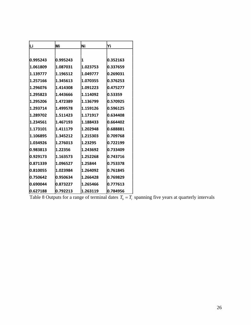
Li Mi Ni Yi 0.995243 0.995243 1 0.352163 1.061809 1.087031 1.023753 0.337659 1.139777 1.196512 1.049777 0.269031 1.257166 1.345613 1.070355 0.376253 1.296076 1.414308 1.091223 0.475277 1.295823 1.443666 1.114092 0.53359 1.295206 1.472389 1.136799 0.570925 1.293714 1.499578 1.159126 0.596125 1.289702 1.511423 1.171917 0.634408 1.234561 1.467193 1.188433 0.664402 1.173101 1.411179 1.202948 0.688881 1.106895 1.345212 1.215303 0.709768 1.034926 1.276013 1.23295 0.722199 0.983813 1.22356 1.243692 0.733409 0.929173 1.163573 1.252268 0.743716 0.871339 1.096527 1.25844 0.753378 0.810055 1.023984 1.264092 0.761845 0.750642 0.950634 1.266428 0.769829 0.690044 0.873227 1.265466 0.777613 0.627188 0.792213 1.263119 0.784956 Table 8 Outputs for a range of terminal dates b iT T= spanning five years at quarterly intervals
27
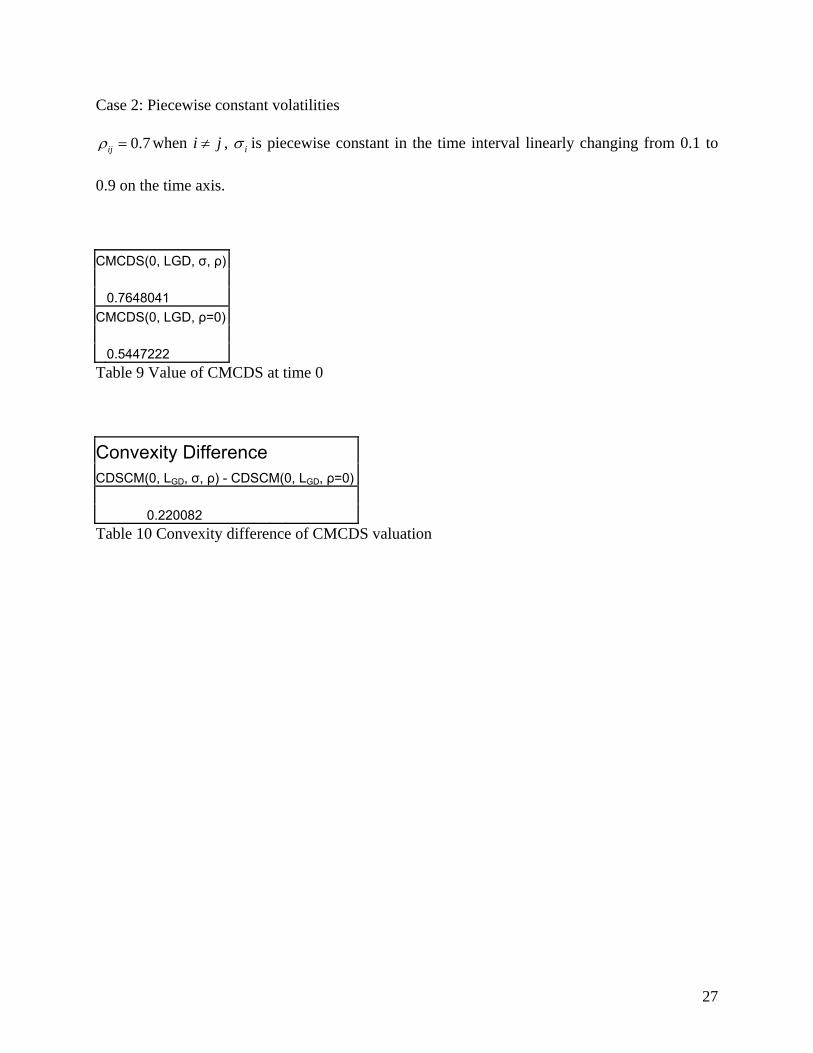
Case 2: Piecewise constant volatilities
0.7ijρ = when i j≠ , iσ is piecewise constant in the time interval linearly changing from 0.1 to
0.9 on the time axis.
CMCDS(0, LGD, σ, ρ) 0.7648041 CMCDS(0, LGD, ρ=0) 0.5447222 Table 9 Value of CMCDS at time 0
Convexity Difference
CDSCM(0, LGD, σ, ρ) - CDSCM(0, LGD, ρ=0)
0.220082 Table 10 Convexity difference of CMCDS valuation
28
Li Mi Ni Yi
0.995243 0.995243 1 0.352163
1.061809 1.097971 1.034056 0.335924
1.139777 1.225954 1.075609 0.265817
1.257166 1.407595 1.119658 0.368418
1.296076 1.525115 1.176717 0.460141
1.295823 1.619376 1.249689 0.509686
1.295206 1.729348 1.335192 0.53707
1.293714 1.852642 1.432034 0.551488
1.289702 1.960995 1.520503 0.577209
1.234561 2.008776 1.627118 0.594787
1.173101 2.02983 1.730312 0.607455
1.106895 2.015768 1.821102 0.617496
1.034926 1.985049 1.918058 0.620776
0.983813 1.937182 1.969056 0.624011
0.929173 1.844003 1.984564 0.627655
0.871339 1.706165 1.958096 0.632004
0.810055 1.537101 1.897528 0.63651
0.750642 1.345477 1.792435 0.641676
0.690044 1.137539 1.648503 0.647587
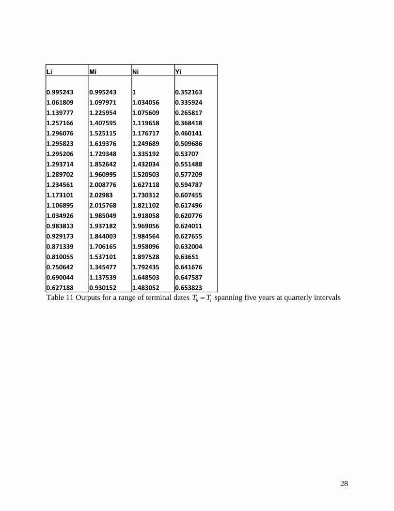
0.627188 0.930152 1.483052 0.653823 Table 11 Outputs for a range of terminal dates b iT T= spanning five years at quarterly intervals
29
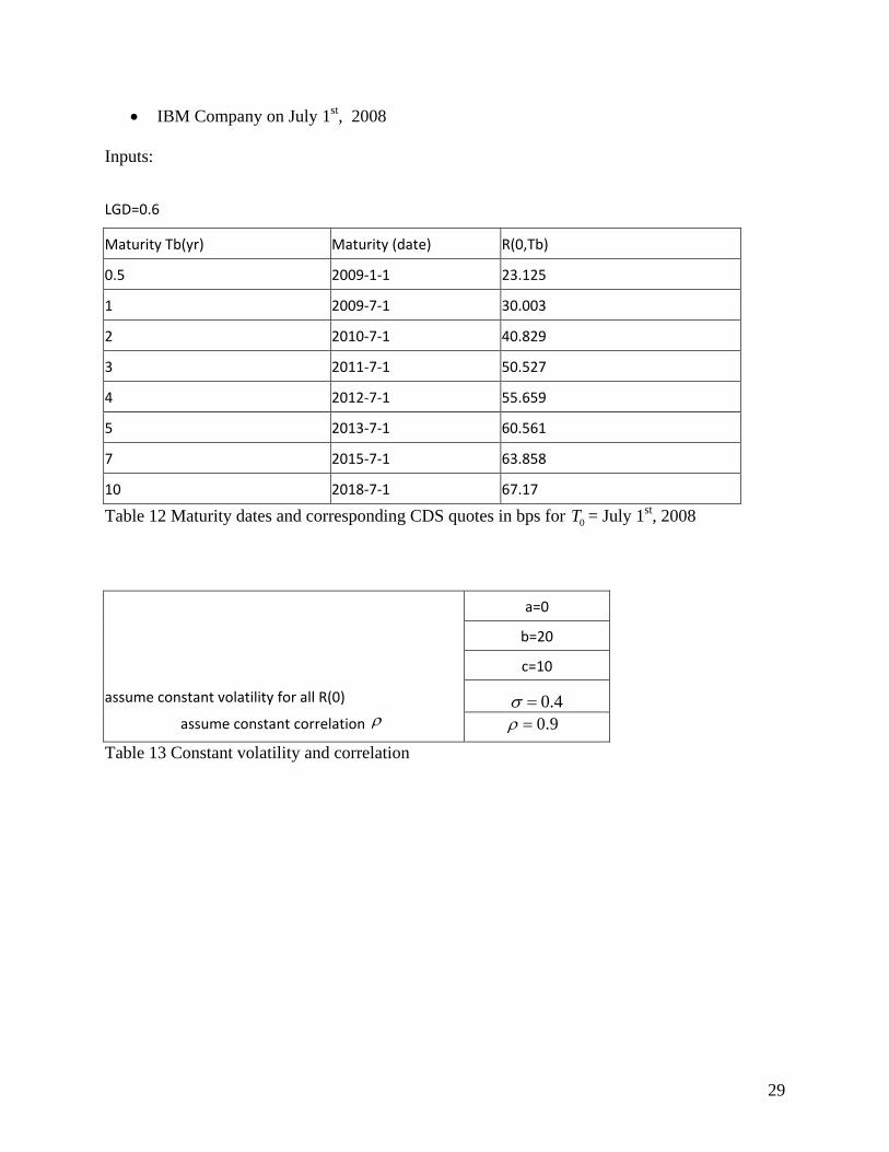
• IBM Company on July 1st, 2008
Inputs:
LGD=0.6 Maturity Tb(yr) Maturity (date) R(0,Tb) 0.5 2009‐1‐1 23.125 1 2009‐7‐1 30.003 2 2010‐7‐1 40.829 3 2011‐7‐1 50.527 4 2012‐7‐1 55.659 5 2013‐7‐1 60.561 7 2015‐7‐1 63.858 10 2018‐7‐1 67.17 Table 12 Maturity dates and corresponding CDS quotes in bps for 0T = July 1st, 2008
a=0 b=20 c=10 assume constant volatility for all R(0) 0.4σ = assume constant correlation ρ 0.9ρ = Table 13 Constant volatility and correlation

30
( )iα iT (0, )iP T ( )iQ Tτ > (0, )iP T ( )iα iT (0, )iP T ( )iQ Tτ > (0, )iP T0.25 0.25 0.99541 99.90% 0.994454 0.25 5.25 0.83575 94.70% 0.7914390.25 0.5 0.98917 99.81% 0.987271 0.25 5.5 0.82607 94.41% 0.7798680.25 0.75 0.98329 99.65% 0.979888 0.25 5.75 0.81633 94.12% 0.7683050.25 1 0.9771 99.50% 0.972215 0.25 6 0.80653 93.83% 0.7567510.25 1.25 0.97062 99.29% 0.96368 0.25 6.25 0.79671 93.54% 0.7452430.25 1.5 0.96384 99.07% 0.954876 0.25 6.5 0.78685 93.25% 0.7337610.25 1.75 0.95679 98.86% 0.945835 0.25 6.75 0.77698 92.97% 0.7223350.25 2 0.94946 98.64% 0.936557 0.25 7 0.76712 92.68% 0.7109820.25 2.25 0.94188 98.35% 0.92633 0.25 7.25 0.75725 92.38% 0.6995630.25 2.5 0.93406 98.06% 0.915921 0.25 7.5 0.74741 92.08% 0.6882450.25 2.75 0.926 97.77% 0.905332 0.25 7.75 0.7376 91.79% 0.6770210.25 3 0.91773 97.48% 0.894594 0.25 8 0.72782 91.49% 0.66589 0.25 3.25 0.90925 97.19% 0.883655 0.25 8.25 0.7181 91.20% 0.6548710.25 3.5 0.90057 96.89% 0.87258 0.25 8.5 0.70842 90.90% 0.6439610.25 3.75 0.89173 96.60% 0.861402 0.25 8.75 0.69882 90.61% 0.6331870.25 4 0.88272 96.31% 0.85013 0.25 9 0.68928 90.32% 0.6225230.25 4.25 0.87356 95.98% 0.838417 0.25 9.25 0.67981 90.02% 0.6119920.25 4.5 0.86427 95.65% 0.82664 0.25 9.5 0.67043 89.73% 0.6015970.25 4.75 0.85486 95.32% 0.814827 0.25 9.75 0.66115 89.44% 0.5913520.25 5 0.84535 94.99% 0.80299 0.25 10 0.65195 89.16% 0.581246
Table 14 Intermediate input of survival probability and defaultable bond price on July, 1st, 2008
31
July-08 July-09 July-10 July-11 July-12 July-13 July-15 July-180.2%
0.4%
0.6%
0.8%
1%
1.2%
1.4%Piecewise Constant Intensity
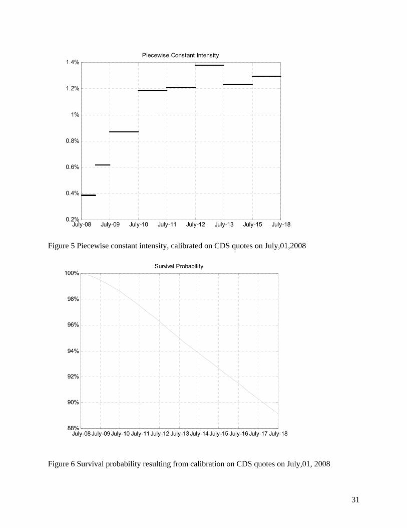
Figure 5 Piecewise constant intensity, calibrated on CDS quotes on July,01,2008
July-08 July-09July-10 July-11 July-12 July-13July-14July-15 July-16July-17 July-18 88%
90%
92%
94%
96%
98%
100%Survival Probability
Figure 6 Survival probability resulting from calibration on CDS quotes on July,01, 2008

32
Outputs:
Case 1: Constant volatility
CMCDS(0, LGD, σ, ρ) ρ 0.7 0.8 0.9 0.99 σ 0.1 0.033044 0.033046 0.033049 0.033051 0.2 0.033093 0.033102 0.033112 0.03312 0.4 0.033291 0.033329 0.033367 0.033401 0.6 0.033626 0.033713 0.0338 0.033879
CMCDS(0, LGD, ρ=0) 0.033028 Table 15 Value of CMCDS at time 0
Convexity Difference CDSCM(0, LGD, σ, ρ) - CDSCM(0, LGD, ρ=0) ρ σ 0.7 0.8 0.9 0.99 0.1 1.63371E-05 1.87E-05 2.1E-05 2.311E-05 0.2 6.54416E-05 7.48E-05 8.42E-05 9.263E-05 0.4 0.000263269 0.000301 0.000339 0.0003735 0.6 0.000598062 0.000685 0.000773 0.0008519 Table 16 Convexity difference of CMCDS valuation
33
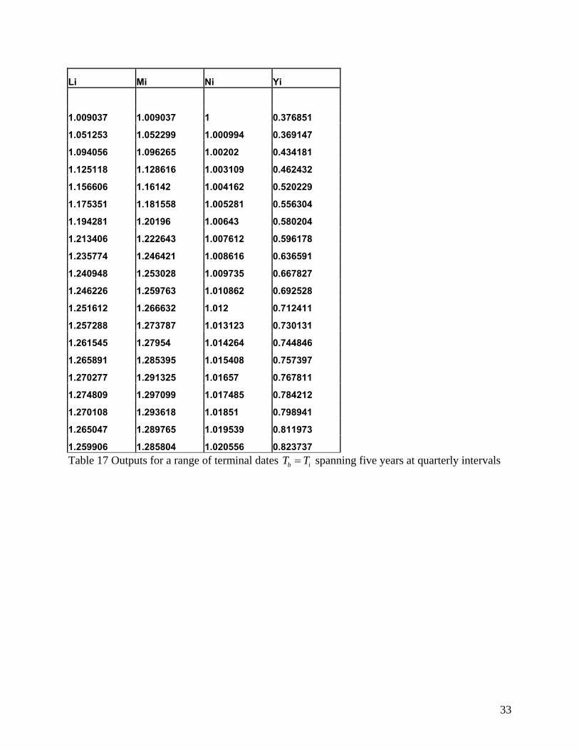
Li Mi Ni Yi 1.009037 1.009037 1 0.376851 1.051253 1.052299 1.000994 0.369147 1.094056 1.096265 1.00202 0.434181 1.125118 1.128616 1.003109 0.462432 1.156606 1.16142 1.004162 0.520229 1.175351 1.181558 1.005281 0.556304 1.194281 1.20196 1.00643 0.580204 1.213406 1.222643 1.007612 0.596178 1.235774 1.246421 1.008616 0.636591 1.240948 1.253028 1.009735 0.667827 1.246226 1.259763 1.010862 0.692528 1.251612 1.266632 1.012 0.712411 1.257288 1.273787 1.013123 0.730131 1.261545 1.27954 1.014264 0.744846 1.265891 1.285395 1.015408 0.757397 1.270277 1.291325 1.01657 0.767811 1.274809 1.297099 1.017485 0.784212 1.270108 1.293618 1.01851 0.798941 1.265047 1.289765 1.019539 0.811973 1.259906 1.285804 1.020556 0.823737 Table 17 Outputs for a range of terminal dates b iT T= spanning five years at quarterly intervals

34
Case 2: Piecewise constant volatilities
0.7ijρ = when i j≠ , iσ is piecewise constant in the time interval linearly changing from 0.1 to
0.9 on the time axis.
CMCDS(0, LGD, σ, ρ) 0.0338529 CMCDS(0, LGD, ρ=0) 0.0330276 Table 18 Value of CMCDS at time 0
Convexity Difference
CDSCM(0, LGD, σ, ρ) - CDSCM(0, LGD, ρ=0) 0.000825 Table 19 Convexity difference of CMCDS valuation

35
Li Mi Ni Yi 1.009037 1.009037 1 0.376851 1.051253 1.053286 1.001933 0.368971 1.094056 1.098661 1.00421 0.433719 1.125118 1.132819 1.006845 0.461621 1.156606 1.167804 1.009681 0.518909 1.175351 1.190415 1.012816 0.554414 1.194281 1.213503 1.016096 0.5777 1.213406 1.236997 1.019441 0.593032 1.235774 1.263513 1.022447 0.632615 1.240948 1.272684 1.025574 0.663012 1.246226 1.281683 1.028451 0.686888 1.251612 1.290389 1.030981 0.705981 1.257288 1.298796 1.033015 0.722953 1.261545 1.30513 1.034549 0.736996 1.265891 1.310789 1.035468 0.748967 1.270277 1.315682 1.035744 0.758913 1.274809 1.319015 1.034676 0.774895 1.270108 1.312094 1.033057 0.789354 1.265047 1.303859 1.03068 0.802278 1.259906 1.294637 1.027566 0.814098 Table 20 Outputs for a range of terminal dates b iT T= spanning five years at quarterly intervals

36
Appendix
Simulation data
1. Default free zero coupon bond price of different maturities for 3 month to 10 years on
July 1st, 2008 and October 28th, 2008
Maturity (yr) 0.25 0.5 0.75 1 1.25 1.5 1.75 2 2008‐7‐10 1.64 2.0955 2.1445 2.1956 2.2488 2.3036 2.3599 2.4173
2008‐10‐28 0.76 1.6734 1.5522 1.4729 1.4329 1.4241 1.4444 1.4874
Maturity (yr) 2.25 2.5 2.75 3 3.25 3.5 3.75 4
2008‐7‐10 2.4758 2.5351 2.5949 2.6553 2.7159 2.7766 2.8373 2.8979
2008‐10‐28 1.5512 1.631 1.7251 1.8298 1.9436 2.0639 2.1893 2.318
Maturity (yr) 4.25 4.5 4.75 5 5.25 5.5 5.75 6
2008‐7‐10 2.9582 3.0182 3.0777 3.1366 3.1949 3.2524 3.3092 3.3651
2008‐10‐28 2.4488 2.5804 2.7117 2.842 2.9703 3.0963 3.2191 3.3386
Maturity (yr) 6.25 6.5 6.75 7 7.25 7.5 7.75 8
2008‐7‐10 3.4201 3.4741 3.527 3.579 3.6298 3.6795 3.728 3.7753 2008‐10‐28 3.454 3.5655 3.6725 3.7751 3.8728 3.9659 4.0541 4.1377
Maturity (yr) 8.25 8.5 8.75 9 9.25 9.5 9.75 10
2008‐7‐10 3.8214 3.8664 3.91 3.9524 3.9935 4.0334 4.072 4.1093 2008‐10‐28 4.2163 4.2904 4.3596 4.4243 4.4844 4.5403 4.5918 4.6392
2. Maturity dates and corresponding CDS quotes
a. IBM Company on October 28th, 2008
Maturity Tb(yr) Maturity (date) R(0,Tb)
0.5 2009‐4‐28 39.1
1 2009‐10‐28 47.327
2 2010‐10‐28 54.669
3 2011‐10‐28 63.894
4 2012‐10‐28 72.652
5 2013‐10‐28 77.16
7 2015‐10‐28 77.472
10 2018‐10‐28 79.439

37
b. IBM Company on July 1st, 2008 LGD=0.6 Maturity Tb(yr) Maturity (date) R(0,Tb) 0.5 2009‐1‐1 23.125 1 2009‐7‐1 30.003 2 2010‐7‐1 40.829 3 2011‐7‐1 50.527 4 2012‐7‐1 55.659 5 2013‐7‐1 60.561 7 2015‐7‐1 63.858 10 2018‐7‐1 67.17
c. Ford Company on July 1st, 2008 LGD=0.6 Maturity Tb(yr) Maturity (date) R(0,Tb) 0.5 2009‐1‐1 700 1 2009‐7‐1 1188.89 2 2010‐7‐1 1664.141 3 2011‐7‐1 1936.845 4 2012‐7‐1 2010.546 5 2013‐7‐1 2043.658 7 2015‐7‐1 1980.742 10 2018‐7‐1 1922.815
3. A sample of VBA Code
Code Sub FindingXi() Const D = 41 Dim Ri(D) Dim DefaultBondPrice(D) Dim alphai(D) Dim Ti(D) sigma = 0 Rho = 0 Lgd = 0

38
'Taking input data from sheet1 For i = 0 To D Ri(i) = Sheet1.Cells(15 + i, 9) 'The values of Ri(0) DefaultBondPrice(i) = Sheet1.Cells(15 + i, 7) alphai(i) = Sheet1.Cells(15 + i, 2) Ti(i) = Sheet1.Cells(15 + i, 3) Next i sigma = Sheet1.Cells(59, 6) Rho = Sheet1.Cells(60, 6) Lgd = Sheet1.Cells(5, 7) a = Sheet1.Cells(6, 7) b = Sheet1.Cells(7, 7) c = Sheet1.Cells(8, 7) 'Finish taking input data from sheet1 Dim ConstantMaturityRate(20) StandardRate = 0 'Finding the Standard Rate Ro,b Using Equation (2) in the paper numerator = 0 denominator = 0 For j = a + 1 To b 'Corresponds to b=20 numerator = numerator + alphai(j) * Ri(j) * DefaultBondPrice(j) denominator = denominator + alphai(j) * DefaultBondPrice(j) Next j StandardRate = numerator / denominator Sheet3.Cells(4, 4) = StandardRate 'Output to Intermediate2 Sheet 'Finish finding the Standard Rate 'Finding Constant Maturity Rate and Calculating Li using Equation (3) and (4) in the paper numerator = 0 denominator = 0 For i = a + 1 To b For j = i To i + c numerator = numerator + alphai(j) * Ri(j) * DefaultBondPrice(j) denominator = denominator + alphai(j) * DefaultBondPrice(j) Next j ConstantMaturityRate(i) = numerator / denominator 'Found the Constant Maturity Rate numerator = 0 denominator = 0 Sheet3.Cells(i + 6, 4) = ConstantMaturityRate(i) 'Output to Intermediate2 Sheet

39
Sheet2.Cells(i + 6, 8) = ConstantMaturityRate(i) / StandardRate Next i
'Finish Finding Constant Maturity Rate and Calculating Li 'Calculating Mi Using Equation (2), (5) and (6) in the Paper Dim YiNumerator(20) winumerator = 0 widenominator = 0 wi = 0 exponential = 0 For j = a + 1 To b For i = j To j + c 'calculating wi For h = j To j + c widenominator = widenominator + alphai(h) * DefaultBondPrice(h) Next h winumerator = alphai(i) * DefaultBondPrice(i) wi = winumerator / widenominator winumerator = 0 widenominator = 0 'Done calculating wi 'Calculating Expected value of Ri(Tj-1) 'Calculating exponential For k = j + 1 To i exponential = exponential + Rho * sigma * Ri(k) / (Ri(k) + Lgd / alphai(k)) Next k exponential = Exp(exponential * Ti(j - 1) * sigma) 'done calculating exponential YiNumerator(j) = YiNumerator(j) + wi * DefaultBondPrice(j) * exponential * Ri(i) 'Expected value of Ri(Tj-1) exponential = 0 Next i Sheet3.Cells(5 + j, 7) = YiNumerator(j) 'Output to Intermediate2 Sheet Sheet3.Cells(5 + j, 12) = DefaultBondPrice(j) * StandardRate 'Output to Intermediate2 Sheet Sheet2.Cells(6 + j, 9) = YiNumerator(j) / (DefaultBondPrice(j) * StandardRate) Next j 'Already have all information for Ni Using Equation (3), (5) and (6) For j = a + 1 To b Sheet2.Cells(6 + j, 10) = YiNumerator(j) / (DefaultBondPrice(j) * ConstantMaturityRate(j)) Sheet3.Cells(31 + j, 3) = DefaultBondPrice(j) * ConstantMaturityRate(j) 'Output to Intermediate2 Sheet Next j
40
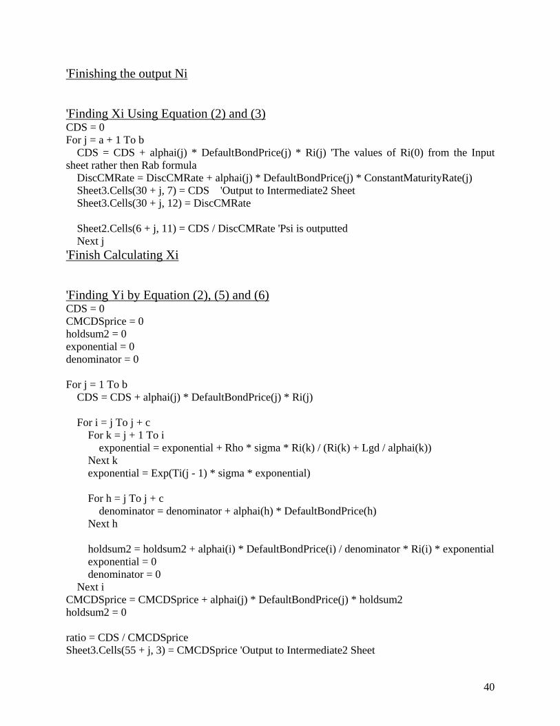
'Finishing the output Ni 'Finding Xi Using Equation (2) and (3) CDS = 0 For j = a + 1 To b CDS = CDS + alphai(j) * DefaultBondPrice(j) * Ri(j) 'The values of Ri(0) from the Input sheet rather then Rab formula DiscCMRate = DiscCMRate + alphai(j) * DefaultBondPrice(j) * ConstantMaturityRate(j) Sheet3.Cells(30 + j, 7) = CDS 'Output to Intermediate2 Sheet Sheet3.Cells(30 + j, 12) = DiscCMRate Sheet2.Cells(6 + j, 11) = CDS / DiscCMRate 'Psi is outputted Next j 'Finish Calculating Xi 'Finding Yi by Equation (2), (5) and (6) CDS = 0 CMCDSprice = 0 holdsum2 = 0 exponential = 0 denominator = 0 For j = 1 To b CDS = CDS + alphai(j) * DefaultBondPrice(j) * Ri(j) For i = j To j + c For k = j + 1 To i exponential = exponential + Rho * sigma * Ri(k) / (Ri(k) + Lgd / alphai(k)) Next k exponential = Exp(Ti(j - 1) * sigma * exponential) For h = j To j + c denominator = denominator + alphai(h) * DefaultBondPrice(h) Next h holdsum2 = holdsum2 + alphai(i) * DefaultBondPrice(i) / denominator * Ri(i) * exponential exponential = 0 denominator = 0 Next i CMCDSprice = CMCDSprice + alphai(j) * DefaultBondPrice(j) * holdsum2 holdsum2 = 0 ratio = CDS / CMCDSprice Sheet3.Cells(55 + j, 3) = CMCDSprice 'Output to Intermediate2 Sheet
41
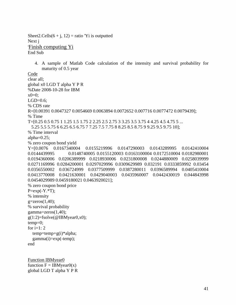
Sheet2.Cells(6 + j, 12) = ratio 'Yi is outputted Next j 'Finish computing Yi End Sub
4. A sample of Matlab Code calculation of the intensity and survival probability for maturity of 0.5 year
Code clear all; global x0 LGD T alpha Y P R %Date 2008-10-28 for IBM x0=0; LGD=0.6; % CDS rate R=[0.00391 0.0047327 0.0054669 0.0063894 0.0072652 0.007716 0.0077472 0.0079439]; % Time T=[0.25 0.5 0.75 1 1.25 1.5 1.75 2 2.25 2.5 2.75 3 3.25 3.5 3.75 4 4.25 4.5 4.75 5 ... 5.25 5.5 5.75 6 6.25 6.5 6.75 7 7.25 7.5 7.75 8 8.25 8.5 8.75 9 9.25 9.5 9.75 10]; % Time interval alpha=0.25; % zero coupon bond yield Y=[0.0076 0.0167340004 0.0155219996 0.0147290003 0.0143289995 0.0142410004 0.0144439995 0.0148740005 0.0155120003 0.0163100004 0.0172510004 0.0182980001 0.0194360006 0.0206389999 0.0218930006 0.0231800008 0.0244880009 0.0258039999 0.0271169996 0.0284200001 0.0297029996 0.0309629989 0.032191 0.0333859992 0.03454 0.0356550002 0.036724999 0.0377509999 0.0387280011 0.0396589994 0.0405410004 0.0413770008 0.0421630001 0.0429040003 0.0435960007 0.0442430019 0.044843998 0.0454029989 0.0459180021 0.0463920021]; % zero coupon bond price P=exp(-Y.*T); % intensity g=zeros(1,40); % survival probability gamma=zeros(1,40); g(1:2)=fsolve(@IBMyear0,x0); temp=0; for i=1: 2 temp=temp+g(i)*alpha; gamma(i)=exp(-temp); end Function IBMyear0 function F = IBMyear0(x) global LGD T alpha Y P R

42
F=R(1)*P(1)*alpha*exp(-x*T(1))+R(1)*P(2)*alpha*exp(-x*T(2))-LGD*x*(exp(-x*T(1))*P(1))*alpha-LGD*x*(exp(-x*T(2))*P(2))*alpha;
References:
1. Damiano Brigo (2006). Constant Maturity Credit Default Swap Valuation with Market Models, Risk, June issue.
2. Damiano Brigo, Fabio Mercurio (2006) The Two-Additive-Factor Gaussian Model G2++. “Interest Rate Models-Theory and Practice With Smile, Inflation and Credit” 2nd edition. Page 170-172
3. Tomas Bjork (2004) Girsanov Theorem. “Arbitrage Theory in Continuous Time” 2nd edition. Page160-167
4. Tomas Bjork (2004) Some Standard Models, The Vasicek Model. “Arbitrage Theory in Continuous Time” 2nd edition. Page 333-334
5. Paul Glasserman (2004), Principles of Monte Carlo. “Monte Carlo Methods in Financial Engineering”. Page 1-38
6. Damiano Brigo, Fabio Mercurio (2006) derivation of Black’s formula. “Interest Rate Models-Theory and Practice With Smile, Inflation and Credit” 2nd edition. Page 200-202
7. Damiano Brigo, Fabio Mercurio (2006).Constant Maturity Credit Default Swaps. “Interest Rate Models-Theory and Practice With Smile, Inflation and Credit” 2nd edition. Page864- 874