Implementation of a Visual SLAM System - Institut de … objective, which is the implementation of a...

Master’s Degree Project Automatic Control and Robotics

Implementation of a Visual SLAM System

Author: Jaime Tarrasó Martínez Director: Joan Solá Ortega Codirector: Juan Andrade Cetto Call: 2015-2

Escola Tècnica Superior

d’Enginyeria Industrial de Barcelona

2

Acknowledgements

I would like to specially thank both my tutors, Juan Andrade Cetto and Joan Solà

Ortega for all the support provided during the whole project.

Special thanks to Joan Vallvé Navarro, who always answers every single one of

my innumerable questions.

Of course, I would really like to thank Fernando Herrero Cotarelo and Sergi

Hernández Juan to put up with every ROS related question I asked.

My most sincere gratitude to the people at IRI, who have helped me greatly.

And last but not least, I would like to thank my family. They have truly been an

inspiration for me.

3

Abstract The goal of this project is to develop a system to compute the position and

orientation of an UAV using a monocular camera. To achieve that, the WOLF library will

be used. WOLF is a library thought to solve generalized simultaneous localization and

mapping (SLAM) and visual odometry problems. Derived classes will implement the

algorithms needed to track features from the images obtained through the sensors.

Constraints between the features and other features, or with landmarks, will be created to

form a factor graph. An external solver will iterate to find the optimal state, by

minimizing the cost associated to all the constraints. Ideally, our system can be used

together with an inertial model measuring rotational velocities and translational

accelerations, and tested with an unmanned aerial vehicle (UAV) in simulation and in

real.environments.

4

Index

Chapter 1 Introduction ........................................................................................................ 6 Chapter 2 Objectives ........................................................................................................... 7 Chapter 3 State of the Art ................................................................................................... 8 Chapter 4 WOLF............................................................................................................... 10

4.1. Introduction to WOLF ........................................................................................... 10 4.2. WOLF tree ............................................................................................................. 11

4.2.1. Problem ........................................................................................................... 12 4.2.2. Map ................................................................................................................. 13 4.2.3. Trajectory ........................................................................................................ 14 4.2.4. Hardware ......................................................................................................... 24

4.3. Solver ..................................................................................................................... 29 4.4. Interaction between the tree ................................................................................... 31

Chapter 5 Visual SLAM contributions ............................................................................ 33 5.1. Introduction ............................................................................................................ 33 5.2. Vision ..................................................................................................................... 33

5.2.1. Tracker ............................................................................................................ 33 5.2.2. Active Search .................................................................................................. 37

5.3. Landmark parametrization: Anchored Homogeneous Point (AHP) ...................... 40 Chapter 6 Implementation in WOLF ............................................................................... 44

6.1. pinholeTools .......................................................................................................... 46 6.2. Sensor Camera ....................................................................................................... 49 6.3. Capture Image ........................................................................................................ 50 6.4. Feature Point Image ............................................................................................... 51 6.5. Landmark AHP ...................................................................................................... 54 6.6. Constraint AHP ...................................................................................................... 56 6.7. Processor Tracker................................................................................................... 60 6.8. Processor Tracker Feature ...................................................................................... 65 6.9. Processor Image Feature ........................................................................................ 70 6.10. Processor Tracker Landmark ............................................................................... 80 6.11. Processor Image Landmark .................................................................................. 83

Chapter 7 Results ............................................................................................................. 90 Chapter 8 Project Management ........................................................................................ 97

8.1. Planning ................................................................................................................. 97 8.2. Costs ....................................................................................................................... 98

Chapter 9 Conclusions ................................................................................................... 101 Chapter 10 Future Work ................................................................................................ 102 Bibliography ................................................................................................................... 103 Appendix ......................................................................................................................... 105

1. changeOfReferenceFrame....................................................................................... 105 2. getLandmarkInReference ........................................................................................ 106 3. pinholeTools operations .......................................................................................... 106

5

4. WOLF code ............................................................................................................. 108

6

Chapter 1

Introduction

One of the biggest challenges for mobile robots is the ability to locate themselves

in the world around them. The task may seem even trivial for us, but for a robot it's a

really complex one.

The ability to know where you are gives you an additional insight on where

everything else really is. Imagine entering a dark room, with only little rays of light

illuminating the barely visible objects inside. Navigating through that space is more

difficult and often forces humans to seek auxiliary sensorial aid.

Mobile robots hardly have that luxury. They must make use of the sensors they

have to know about their environment, as efficient as possible. And they must navigate

through that environment, as safely as possible. Knowing what is around yourself, and

your position in relation to them is the key to an efficient, yet safe, navigation.

The simultaneous localization and mapping (SLAM) problem tackles this issue.

It tries to simultaneously locate itself while exploring the environment. The ramifications

of this problem are many and diverse, as one can use many different sensors to explore

the surroundings. Moreover, the movement of the robot can also vary, depending on the

robot's design, and must be taken into account when computing the motion.

7

Chapter 2

Objectives

The ultimate objective of this project is to develop and implement a visual-inertial

odometry or SLAM system for a UAV platform. We however concentrate on a part of

this objective, which is the implementation of a visual SLAM algorithm that accurately

computes the motion of a robot by integrating information from a camera.

Contributions to the WOLF library (Windowed Localization Frames) will be

developed to achieve the objectives of this project. This library is a collaborative project

at the Institut de Robòtica i Informàtica Industrial (IRI) that solves various types of

localization problems as the optimization of a network of geometric constraints, and can

be used to find solutions to localization, SLAM, or odometry problems, using any kind of

sensor modality.

The goal of this project is, by means of the WOLF library, to implement a system

that is able to compute the position and orientation of an UAV via camera sensors.

8

Chapter 3

State of the Art

The simultaneous localization and mapping (SLAM) problem tackles two

different and complementary problems at the same time. A robot needs to explore an area

often with a blank map, while trying to know its location as it moves. To a certain degree

it is funny, as one of the tasks gets in the way of the other: you can’t explore and map the

environment efficiently if you don’t know your position in this environment, but to be

able to locate yourself requires exploring and mapping the surroundings. The problem of

simultaneous localization and mapping is therefore central to autonomous navigation.

We must approach this immense problem with a clear mindset: get real time

execution and robustness. Among many other sensor modalities, which include laser

scanners, sonar, radar, stereo cameras, or RGBD sensors, one of the most

challenging problems is to perform localization and mapping using single cameras,

extracting the features and applying a motion modelling. The Extended Kalman Filter

(EKF) has been for many years the preferred method in many SLAM estimation

problems like these, with good solutions in feature and landmark initialization (Davison,

2003). The EKF is able to fuse the motion estimation with the measurements, and obtain

an accurate estimation of the position of the robot, as well as the landmark initialization

(Roussillon et al., 2011). The monocular camera can be effectively used to estimate the

motion by detecting and tracking features through the stream of images (Wang et al.,

2012), or relegate obtaining the motion to an inertial measurement unit (IMU). (Mostofi,

Elhabiby, & El-Sheimy, 2014)

9

A different, more modern approach, while also using cameras is to obtain visual

motion estimation through keyframes, and perform a non-linear optimization over all the

keyframes and landmarks (Konolige, Agrawal, & Solà, 2011). In these approaches, the

algorithm selects on a reduced number of past frames to process, known as keyframes,

which capture the structure of the trajectory of the robot, yet it is sparse enough to avoid

highly redundant measurements in the system to solve. This, together with techniques for

incrementally updating and solving the problem as the robot moves and gathers new

information, makes this method fast and robust, and suitable for systems that have fixed

computational bounds, as it is often the case for mobile robots (Strasdat, Montiel, &

Davison, 2010). This is the approach taken in this thesis.

10

Chapter 4

WOLF

4.1. Introduction to WOLF

To achieve the proposed objectives we will use a library created to solve

localization problems in mobile robotics called WOLF (Windowed Localization Frames).

This library is able to solve SLAM (Simultaneous Localization And Mapping), map-

based localization or visual odometry problems and, with that in mind, this project will

use to its advantage the structure of WOLF and its resources.

The WOLF library is mainly a tool to organize and store the data of the problem.

The state vector to be estimated is formed by keyframes, plus other states like landmarks

or sensor parameters.

The main WOLF structure, called "WOLF tree", reproduces the elements of the

robotic problem: The robot trajectory formed by keyframes, a potential wide range of

sensors and a map with landmarks. With WOLF this data can be easily accessed and

organized, albeit it requires external aid to successfully operate, with elements as input

sensors (one or multiple sensors) or a solver to compute the result. WOLF may be

interfaced with many kinds of solvers, including filters and nonlinear optimizers (such as

a wide variety of Kalman Filters), and it also can be used with nonlinear optimizers. To

interact with these solvers WOLF relegates the task to wrappers, so that the library is not

bound to any solver. The library currently provides a wrapper to the Google Ceres solver.

WOLF reproduces the elements of a robotic problem by means of a tree of base

classes. These base classes form the main structure that can be derived to build the

11

particularizations needed for the problem, as the base functionality is embedded in the

base classes, and anything derived from them can add whatever it is necessary.

One of the main advantages of using the WOLF tree is the connectivity along its

branches, as it works in both directions: from parent to child and from child to parent.

This way, the information of the parent elements in the branch can be accessed by any of

the children. Moreover, this connectivity is highlighted when using constraints linking

different parts of the tree, creating a graph of states.

This graph of states, linking state blocks with constraints is equivalent to the

factor graph that would be solved non-linear optimization. The wrappers will translate the

information stored in the WOLF tree into a factor graph that can be understood by the

selected solver.

This chapter is meant to explain the WOLF library and its main classes and

functions. Since, as it was previously said, WOLF is meant to be used as a generalized

SLAM library, the main algorithm uses base classes. With that in mind we create derived

ones, to suit the purposes of the problem at hand. In this project, and in order to explain

without confusing terms, the specific explanation of the derived classes will be done in

one of the following chapters, leaving the present one with the more general base classes.

4.2. WOLF tree

The main structure of the library is called "WOLF tree". It manages and organizes

the data of the problem and makes it easy to access. The tree in its entirety can be seen in

Figure 1.

12

Above all the other classes in the tree we find the Problem class. From there, the

tree branches to organize the data, with each class of a branch containing more specific

information than the previous one, making it accessible due to its disposition.

4.2.1. Problem

While the Problem class is not the hierarchical upper class of the WOLF library,

as there are others above it for managing purposes, it is the visible upper class from the

user standpoint. It doesn't have much real impact in the development of the project, as its

main functionality serves more to organize and manage the data of the lower classes, but

there has to be a class at the top of problem, as well as a main class from which all

derives.

Figure 1 - The WOLF tree.

13

From this class the three distinctive branches of the tree appear: The problem's

Hardware, the robot's Trajectory, and a Map of Landmarks.

4.2.2. Map The Map class is merely a list of any kind of Landmarks. It stores them so that the

solver can use the information of all the Landmarks (among other things) to calculate the

position of the robot. Since it is such a simple class, it has two main functions aside the

constructor: addLandmark and removeLandmark, which add or remove landmarks from

the class.

Though it may seem that the Map class should incorporate some functions to

actively interact with the landmarks it stores, that kind of operation has to be defined by

the Processor and, thus, defined in the derived Processor class. (which will be explained

later on). As mentioned before, the only objective of this class is to store Landmarks. Any

operation or function using Landmarks in any way should be done elsewhere, by another

class.

Figure 2 - The Map branch Figure 2 - The Map branch

14

4.2.2.1. Landmarks

The Landmark class defines a geometric feature of the environment. Though each

derived class may have their own particular variables and functions, the base class has the

following general elements:

unsigned int landmark_id_; ///< landmark unique id LandmarkType type_id_; ///< type of landmark. (types defined at wolf.h) LandmarkStatus status_; ///< status of the landmark. (types defined at wolf.h) TimeStamp stamp_; ///< stamp of the creation of the landmark StateBlock* p_ptr_; ///< Position state block pointer StateBlock* o_ptr_; ///< Orientation state block pointer

The first fourth variables are just managing variables. The only purpose they

serve is to assign a number to the landmark, specify the type of landmark it is (any

derived class of landmark), its status and the time in which it was created.

The other two variables are more important. They are StateBlocks pointers which

store the information concerning position and orientation of the landmark. The

StateBlock is a partition of the state vector of the problem, and thus is meant to store the

most important data in the project.

Aside these variables, there are also base functions. The most important ones are

the ones to modify or read the values of the variables (such as setId or getPPtr ).

4.2.3. Trajectory

The Trajectory branch holds all the data in respect of the movement of the robot.

To do that, it has different levels of organization, essential to keep everything organized

and to perform the calculation of the residual error.

15

Since this class is one of the three main branches of the Problem class, most of its

functions are used by the upper classes to manage the Frame class below, so all the

information in this branch is sorted and organized for other classes to access. The two

most used functions are getLastFramePtr, which will return a pointer to the last Frame,

and getFrameListPrt, which returns a pointer to the list of Frames the Trajectory class

holds.

4.2.3.1. Frame

The Frame class is just below the Trajectory. The main function of this class is to

keep the information of the robot state at different moments in time. For each given time

Figure 3 - The Trajectory branch

16

a Frame is created, varying its type depending on the Processor: A 'NON-KEYFRAME'

Frame object, and a special category of Frames labeled 'KEYFRAME'. The Processor

class is the one who decides which Frames are made into a keyframe and which are not,

and only keyframes are the ones entering in the optimization solver and thus used to

solve the problem.

unsigned int frame_id_; ///< id of the frame FrameKeyType type_id_; ///< type of frame. Either NON_KEY_FRAME or KEY_FRAME. (types defined at wolf.h) TimeStamp time_stamp_; ///< frame time stamp StateStatus status_; ///< status of the estimation of the frame state StateBlock* p_ptr_; ///< Position state block pointer StateBlock* o_ptr_; ///< Orientation state block pointer StateBlock* v_ptr_; ///< Linear velocity state block pointer

Following the same structure as the Landmark class, most variables are used to

store information about the Frame itself. There is a "id" to assign a number to any Frame,

it is also defined which type of Frame it is (NON-KEYFRAME or KEYFRAME), as well

as the moment in time in which said Frame is created and its current status. Those

variables are used mostly by upper management classes. The most important variables in

regard to this project are the three StateBlock pointers (the importance of this new class

will be explained along the Solver, in Chapter 4.3). Each one of them returns a pointer to

the position, orientation and linear velocity of the Frame, which is used by WOLF to

solve the problem, as well as for correctly placing all the Capture and Feature objects

below in the WOLF tree.

17

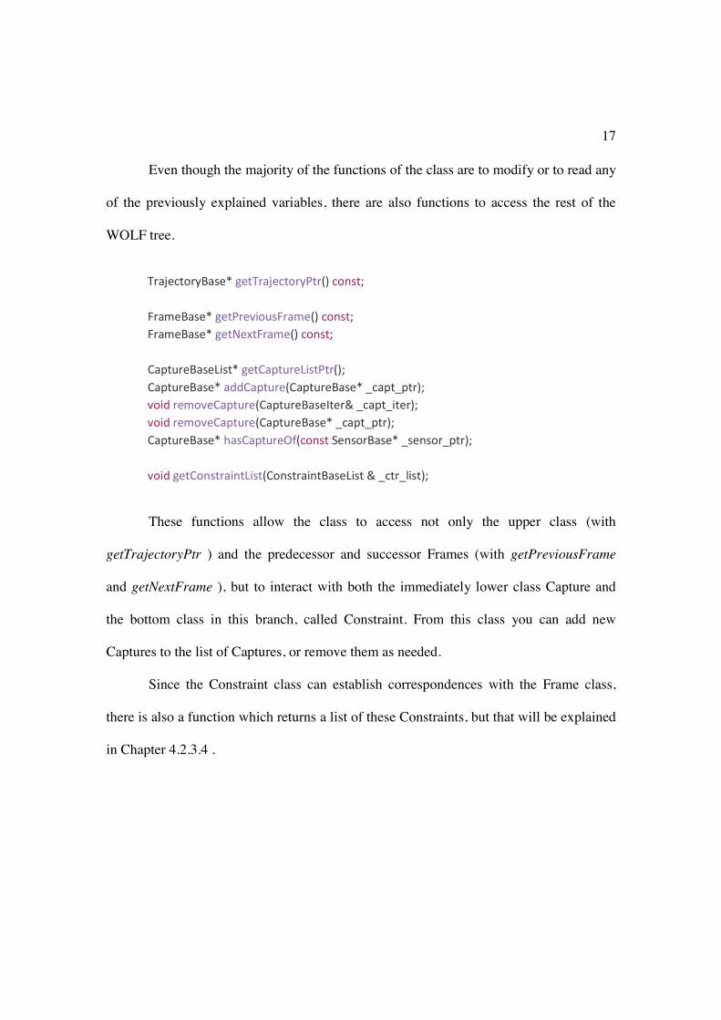
Even though the majority of the functions of the class are to modify or to read any

of the previously explained variables, there are also functions to access the rest of the

WOLF tree.

TrajectoryBase* getTrajectoryPtr() const; FrameBase* getPreviousFrame() const; FrameBase* getNextFrame() const; CaptureBaseList* getCaptureListPtr(); CaptureBase* addCapture(CaptureBase* _capt_ptr); void removeCapture(CaptureBaseIter& _capt_iter); void removeCapture(CaptureBase* _capt_ptr); CaptureBase* hasCaptureOf(const SensorBase* _sensor_ptr); void getConstraintList(ConstraintBaseList & _ctr_list);

These functions allow the class to access not only the upper class (with

getTrajectoryPtr ) and the predecessor and successor Frames (with getPreviousFrame

and getNextFrame ), but to interact with both the immediately lower class Capture and

the bottom class in this branch, called Constraint. From this class you can add new

Captures to the list of Captures, or remove them as needed.

Since the Constraint class can establish correspondences with the Frame class,

there is also a function which returns a list of these Constraints, but that will be explained

in Chapter 4.2.3.4 .

18

4.2.3.2. Capture

In each Frame there is a list of Captures. The Capture class is an object with the

purpose to store the raw data obtained by the sensor, as well as to maintain a list of

Features found in said data. Since the type of the sensor can vary, this class will also

change to accommodate. However, even though Captures of different sensors may

present different structures, some variables and functions must remain unchanged to

support the WOLF tree structure.

! Variables

unsigned int capture_id_; TimeStamp time_stamp_; SensorBase* sensor_ptr_; StateBlock* sensor_p_ptr_; StateBlock* sensor_o_ptr_;

It has an "id" to easily indentify the object, as most of the classes in the WOLF

tree, and a time stamp with the time at which it was created. The base class also has a

pointer to the Sensor class the Capture was extracted from, since the WOLF library

allows for multiple sensors at the same time, as well as the pointer to said sensor position

and orientation.

! Functions

The functions used in the base class are mainly to read the previously explained

variables. There are, however, some other functions that should be mentioned.

19

FeatureBase* addFeature(FeatureBase* _ft_ptr); FrameBase* getFramePtr() const; FeatureBaseList* getFeatureListPtr(); void getConstraintList(ConstraintBaseList & _ctr_list); virtual void process();

From this class you can access the Frame class above with getFramePtr. Using

the function addFeatures the class can add the Features found in the data stored in the

class, and to the list of Features (getFeatureListPtr).

The Constraint class can't create correspondences with the Capture class (as it did

with the Frame class), but there is a function which returns a list of these Constraints,

which will be explained in Chapter 4.2.3.4 .

The last function, called "process" will require a more in-depth explanation:

void CaptureBase::process(); { // Call all processors assigned to the sensor that captured this data for (auto processor_iter = sensor_ptr_->getProcessorListPtr()->begin(); processor_iter != sensor_ptr_->getProcessorListPtr()->end(); ++processor_iter) { (*processor_iter)->process(this); } }

The main goal of the function is to initiate the processing of the raw data. Though

there are multiple methods to initiate the Processor class, this one is the method which

makes more sense. As you can see in the code, the Capture class will search for all the

Processor classes inside the Sensor the data has been acquired from. The Processor will

start analyzing the data.

20

It may seem a convoluted method to initiate the process but in this way we assure

that the process is called only when there is data to analyze, and in no other case. Further

explanation on the process() function in the Process class, Chapter 4.2.4.2 .

4.2.3.3. Feature

The main objective of the Feature class is to store a particular metric

measurement from the raw data in the Capture class.

! Variables

unsigned int feature_id_;

unsigned int track_id_;

unsigned int landmark_id_;

FeatureType type_id_;

Eigen::VectorXs measurement_;

Eigen::MatrixXs measurement_covariance_;

Eigen::MatrixXs measurement_sqrt_information_;

This class has three identification numbers. The first one, "feature id" is the one

that will number itself, while the other two, "track id" and "landmark id", will be set if

the feature has been tracked or successfully associated with a Landmark. There is also a

variable to identify which type of Feature is being used, as it undoubtedly be one of the

derived classes.

The Feature class stores information in the three different variables: the

measurement, which is a vector of dynamic nature to adequate to whatever kind of value

is sent by a derived class, a measurement covariance with the covariance of said

measurement, and one variable called "measurement_sqrt_information_", which will

operate the square root of the inverse of the covariance using Eigen functions. The

21

inverse of the covariance is called "Information", and that square root matrix can be

defined by the Cholesky decomposition. The information matrix is needed when

computing the residual error of the position of the robot, and since it's a constraint it is

done in this particular class to ease the computational cost that would be calculating that

value when it's requested.

! Functions

As with most of the previous classes, the majority of the functions are to either to

read or to modify the values in the variables. With the exception of those, the most

important functions are these:

ConstraintBase* addConstraint(ConstraintBase* _co_ptr);

CaptureBase* getCapturePtr() const;

FrameBase* getFramePtr() const;

ConstraintBaseList* getConstraintListPtr();

void getConstraintList(ConstraintBaseList & _ctr_list);

These functions are, just as any other class, allowing connectivity in the WOLF

tree. They allow the access to parent classes (such as Capture and Frame), as well as to

interact with the child class, Constraint. More in detail of this last functionality, the

Feature class is allowed to add Constraints, as well as to see the Constraint list.

4.2.3.4. Constraint

The Constraint class' main purpose is to establish a correspondence between a

Feature and another element from the WOLF tree, which can be a Frame, a Landmark or

another Feature. To be more specific, the Constraint is a link between State Blocks to

22

compute an error, and will be used by the solver to minimize the global error of the

system, thus achieving the optimal state. This is one of the most important classes in the

WOLF structure. It's the one to compute the residual error, and the code optimization

when doing so is completely mandatory.

! Variables

unsigned int constraint_id_;

ConstraintType type_id_; ///< type of constraint (types defined at wolf.h)

ConstraintCategory category_; ///< category of constraint (types defined at wolf.h)

ConstraintStatus status_; ///< status of constraint (types defined at wolf.h)

bool apply_loss_function_; ///< flag for applying loss function to this constraint

FrameBase* frame_ptr_; ///< FrameBase pointer (for category CTR_FRAME)

FeatureBase* feature_ptr_; ///< FeatureBase pointer (for category CTR_FEATURE)

LandmarkBase* landmark_ptr_; ///< LandmarkBase pointer (for category CTR_LANDMARK)

This class has five variables to store information about the Constraint, such as the

"id", the type (to know which derived class is currently in use), category (which

identifies the type of correspondence made, varying between four categories:

'ABSOLUTE', 'FRAME', 'FEATURE' and 'LANDMARK') and the status of the

Constraint. There is also a boolean variable which decides if the Constraint will apply

"loss function".

The other three variables have a pointer to each one of the three possible types of

elements the Constraint can link the Feature to.

23

! Constructor

In this class there are four constructors: one for each type of category available

(Frame, Feature or Landmark) as well as one for an 'ABSOLUTE' category, in which the

Constraint is created but a correspondence is not made with another element.

/** \brief Constructor of category CTR_ABSOLUTE **/

ConstraintBase(ConstraintType _tp, bool _apply_loss_function, ConstraintStatus

_status);

/** \brief Constructor of category CTR_FRAME **/

ConstraintBase(ConstraintType _tp, FrameBase* _frame_ptr, bool _apply_loss_function,

ConstraintStatus _status);

/** \brief Constructor of category CTR_FEATURE **/

ConstraintBase(ConstraintType _tp, FeatureBase* _feature_ptr, bool

_apply_loss_function, ConstraintStatus _status);

/** \brief Constructor of category CTR_LANDMARK **/

ConstraintBase(ConstraintType _tp, LandmarkBase* _landmark_ptr, bool

_apply_loss_function, ConstraintStatus _status);

As a side note, it is important to mention that, in case the Constraint is about to be

erased, or one of the two links in the Constraint is, the WOLF algorithm would check if

the other part of the correspondence needs to be erased as well, to maintain the stability

and the organization in the tree. This is automatically done by WOLF in their respective

base class.

! Functions

The functions in this class are meant to retrieve or to modify existing values of the

variables, as well as pointers to all the possible categorized elements linked in the

Constraint.

24

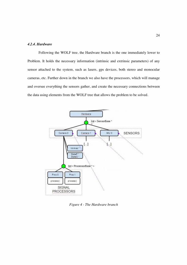
4.2.4. Hardware

Following the WOLF tree, the Hardware branch is the one immediately lower to

Problem. It holds the necessary information (intrinsic and extrinsic parameters) of any

sensor attached to the system, such as lasers, gps devices, both stereo and monocular

cameras, etc. Further down in the branch we also have the processors, which will manage

and oversee everything the sensors gather, and create the necessary connections between

the data using elements from the WOLF tree that allows the problem to be solved.

Figure 4 - The Hardware branch

25

4.2.4.1. Sensor

The Sensor sub-branch is immediately after the Hardware class. Its main function

is to store all the essential values from the available sensors that will be needed during the

execution of the algorithm, such as intrinsic and extrinsic parameters, among others.

! Variables

unsigned int sensor_id_;

SensorType type_id_;

StateBlock* p_ptr_;

StateBlock* o_ptr_;

StateBlock* intrinsic_ptr_;

Eigen::VectorXs noise_std_;

Eigen::MatrixXs noise_cov_;

As all the previous classes, this one has its own identification number, as well as a

type which corresponds to the sensor that will be used. It has two State Blocks to keep the

values of the position and orientation of the sensor, and also another one to store its

intrinsic parameters. The sensor noise and the covariance of that noise are also taken into

account. This way all the necessary information about the Sensor is available for any

class that needs it.

! Functions

The functions of the class are more or less standard, as the majority of them have

the purpose of modifying or reading the stored value, such as getPPrt, which is used to

return a pointer to the StateBlock position.

26

The two functions that stand out in this class are the following:

ProcessorBase* addProcessor(ProcessorBase* _proc_ptr);

ProcessorBaseList* getProcessorListPtr();

These functions allow for the Sensor to interact with the Processor class, in the

way that it can add a Processor and get the list of Processors currently hanging from the

sensor.

4.2.4.2. Processor

The class below the Sensor class is that of the Processor. The importance of this

class within the whole WOLF tree is incredibly high, as its main goal is to direct how the

whole problem is solved. The class has to extract information from the sensors and

analyze the result, so connections can be made in order to solve the problem.

If one doesn't know how the WOLF tree works, it may seem confusing why such

an important class is "hanging" from the Sensor class, and not in a more higher position

in the tree. The answer is simple: The methodology to analyze the problem is directly

dependant on how to access that information, and the way to interact with the real

environment is through the sensors. For example, the methodology a processor must

follow to analyze a GPS sensor greatly differs from the methodology used in a camera

sensor. Also, the WOLF library is, as it has been mentioned before, a generalized way to

approach SLAM problems. And, of course, a real world SLAM problem may be solved

by one or more sensors at the same time. That has also to be taken into account,

reinforcing the idea that the Processor class should be below the Sensor class.

27

There are, however, some architecture decisions to note. Each Processor can only

hang from one Sensor, as the procedure followed in this class is heavily influenced by the

nature of the Sensor above. On the other hand, many Processors can hang from one

Sensor (though not necessarily), as the Processor class envelops a methodology and, as

such, there can be other methodologies for the same task. An example of this could be

two different Processors hanged from the same camera sensor, with the peculiarity that

each one of these two Processors has a different approach to the problem: one extracts

points from the image, and the other extracts lines. Their procedures are different, but the

Sensor providing them with raw data is the same.

! Variables

unsigned int processor_id_;

ProcessorType type_id_;

Scalar time_tolerance_; ///< self time tolerance for adding a capture into a frame

The main variables of this class are just identification numbers for either the

Processor or the type of Processor in use. There is also a time tolerance variable to assure

that one of the main functions, called MakeFrame, is performing as it should.

! Functions

This class is meant to be derived, and use the functions here to implement a more

specific and adequate procedure for the whole problem. Therefore, most of the functions

in this Processor Base class are "pure virtual", which means that even though they are

created here, the functionality has to be implemented in the derived classes. This way, the

base class forces the derived ones to do certain functions and protect the integrity of

WOLF tree at the same time.

28

virtual void process(CaptureBase* _capture_ptr) = 0; virtual bool voteForKeyFrame() = 0; virtual bool permittedKeyFrame() final; virtual void makeFrame(CaptureBase* _capture_ptr, FrameKeyType _type = NON_KEY_FRAME);

The process function is, without a doubt, the main function of the whole WOLF

tree. It is the one that orchestrates and commands the other classes so that a solution can

be achieved. The derived classes must define there a methodology to analyze the data

obtained from the sensors and, using the whole WOLF tree structure, create a graph of

Constraints through the tree.

Another important function is the one called voteForKeyFrame. Keyframes are a

very special subset of the Frame class. They are the only ones in which the external

solver will focus to find a solution. Therefore, a nice strategy must be implemented in the

derived classes to decide when a new keyframe must be created. It can be simple or really

complex, but the function must be there to decide, hence making it a pure virtual

function.

Along with that function there is another called permittedKeyFrame, the purpose

of which is to simply dictate if a keyframe can be created or not. It it's not allowed in this

function, even if voteForKeyFrame decides that it is needed, it won't be created.

The makeFrame function is quite straightforward in its main purpose: create a

new Frame. It is important to mention that, due to the way the WOLF tree is conceived, a

Frame has to have a Capture hanging from it. The Frame must have something below to

be created. If there is no data, there is no reason to create a new Frame. That is why there

29

is a Capture class as input in the function, as well as the type of Frame we want to create

(by default it is set at 'NON-KEYFRAME').

4.3. Solver

To find a solution to the problem WOLF uses an external solver. It is not part of

the library itself, but works alongside with it, as it's a necessary element in this non-linear

optimization problem. The wrapper will interact between the solver and the WOLF

structure, to make one independent from the other.

Figure 5 - Outside of WOLF

The WOLF tree interaction with the solver is done though State Blocks and

Constraints. As it has been mentioned before, the State Blocks are partitions of the state

vector, containing all the important information of this project, while the Constraints are

just links between the State Blocks.

30

In the following factor graph the round nodes, labelled from 0 to 7 in the Figure,

are State Blocks, while in square nodes, labelled from 1 to 10, represents the Constraints.

Figure 6 - Factor Graph of StateBlocks and Constraints

For each of the Constraints, a residual is calculated, using information from the

State Blocks and measurements. This residual, also known as "expectation error", is used

by the solver in order to find the overall state that minimizes it, obtaining the optimal

state, which is the best available solution for the problem. The solver's procedure to solve

this problem is it follows:

1. Linearize all the Constraints

2. Compute an optimal state correction of the linearized system

3. Update the state with the correction step

4. Iterate from 1 until convergence

31

The operations 2 to 4 are done automatically by the solver, but the task to

linearize the Constraints must be done by WOLF. At each iteration the solver will ask to

each constraint:

1. A value of the Constraint residual

2. If applicable, a Jacobian of said residual, with respect to each of the State Blocks.

The math behind the calculation of the residual in the Constraint is fairly simple,

as WOLF organizes and stores the data to have an easy access to the measurements and

State Blocks needed for that.

4.4. Interaction between the tree

As the classes and functions used by the base WOLF tree have now been

explained, a summary of the methodology of WOLF should be in order.

Figure 7 - Illustration of a working WOLF test

32

The whole process starts when a Capture is introduced by one of the Sensors. It is

stored below a Frame along with the position and orientation of the robot at that

particular moment. At the umpteenth iteration we will have a Trajectory of Frames, just

as the one in Figure 7.

To better understand the relationship between the tree, we will explain an

example of a mobile robot detecting Landmarks.

In every iteration, the Capture is analyzed by the Processor, finding recognizable

Features in it. Landmarks are made from those Features and, in each passing iteration,

those Landmarks may (or may not) be found in the Capture. Every time they are

recognized, a Constraint is made between the Feature and the Landmark.

When the Processor so decides it, some of the Frames are made into keyframes.

When the time is right, those are sent to the external solver, which asks for the residual in

each of the created Constraints. If the solver converges, that means that the residual has

been minimized, and an optimal state has been found, localizing as best as it can the robot

and the Landmarks. This gives more precise calculations for further iterations.

33

Chapter 5

Visual SLAM contributions

5.1. Introduction

In mobile robotics, the SLAM problem can be summarized as the localization of

the robot and, at the same time, the mapping of the environment around it. To fulfil that

objective sensors are needed to gather information about the world. In the current project

we will work with a camera sensor, so certain visual elements must be included to

properly analyze the image. Moreover, we must specify the way in which we map the

environment, and so, there must be an explanation of how we parametrize a Landmark.

5.2. Vision

In this project we will be using a monocular camera to recognize the environment

and to create and track either Landmarks and Features. The sensor supplying the raw data

will be a camera and, in consequence, we will need to analyze images and extract

keypoints to create Features.

5.2.1. Tracker

Among the many keypoints detectors there are available nowadays, four names

stood out from the rest: SIFT, SURF, ORB and BRISK. The first two have been used for

many years, and give really high performance with remarkable and detailed keypoints,

albeit consuming a lot of computational cost in the process. The other two, ORB and

BRISK are relatively new and, with a slightly lesser keypoint detection performance, they

offer a dramatically faster alternative.

34

It was decided to use ORB and BRISK instead of the trustworthy alternative to

prioritize speed, as the keypoint detection is just one of the many parts of the project, and

the solver iterations already consume large quantities of the computational time.

Moreover, they are available in the OpenCV library and come with wide range of

functions and methods to apply keypoint detection, description and matching.

! Detection

The BRISK keypoint detector is based on another keypoint detector technique

called FAST. It looks for a maxima in the image plane and, to achieve invariance to

scale, also in the scale-space using as threshold the score of the FAST detector,

measuring the saliency of the keypoint. (Leutenegger, Chli, & Siegwart)

Figure 8 - BRISK using FAST to obtain a keypoint

35

BRISK uses a 9-16 mask to perform the detection, which means that in a circle of

16 pixels at least 9 in consecutive form have to be either darker or brighter than the

analyzed point. If that criterion is validated BRISK will search in the above and below

layer, in which the values have to be lower too. There layers are called octaves, and are

created from the original image, each one being a half-sample of the previous one.

The ORB detector also uses FAST to detect keypoints, combined with the Harris

corner measure. A scale pyramid of the image is created to produce FAST features in

each one of the layers of said pyramid, previously filtered by Harris. If the keypoints

have a FAST value over a set threshold, they are chosen. Then, using a technique called

"intensity centroid" they are able to find the orientation of the feature, which will be of

use when describing the keypoints. (Rublee, Rabaud, Konolige, & Bradski)

In the project, as the OpenCV library has these two detectors, and just using the

function detect with an image (or a region of interest of that image) it will find a list of

keypoints.

! Description

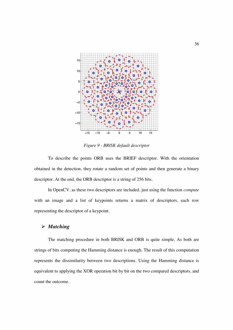
The BRISK descriptor uses by default a circular sampling pattern of 60 points and

it separates them into two subsets: long-distance and short-distance pairs. It computes the

local gradient for the long-distance pairs and sums the gradient to find the orientation of

the feature. Then rotates the short-distance pairs the same amount and constructs a binary

operator using these pairs. The description of a keypoint in BRISK presented as a string

of 512 bits.

36

Figure 9 - BRISK default descriptor

To describe the points ORB uses the BRIEF descriptor. With the orientation

obtained in the detection, they rotate a random set of points and then generate a binary

descriptor. At the end, the ORB descriptor is a string of 256 bits.

In OpenCV, as these two descriptors are included, just using the function compute

with an image and a list of keypoints returns a matrix of descriptors, each row

representing the descriptor of a keypoint.

! Matching

The matching procedure in both BRISK and ORB is quite simple. As both are

strings of bits computing the Hamming distance is enough. The result of this computation

represents the dissimilarity between two descriptions. Using the Hamming distance is

equivalent to applying the XOR operation bit by bit on the two compared descriptors, and

count the outcome.

37

In OpenCV, the function match (although previously parametrized) can compute

the Hamming distance between sets of descriptors.

5.2.2. Active Search

Even with those vision systems, tracking is not a simple thing to achieve.

Analyzing the whole image may be a computational cost far too high for a robotic

problem, especially if the characteristics of the image are not known when designing it.

And, since WOLF is designed to work with any kind of sensor, it may work with any

kind of image. Therefore, we must localize and define where to search in order to reduce

the computational time. To do that we will use Active Search.

Originally designed in the RTSLAM project, from LASS, the Active Search class

was adapted to WOLF by a Dinesh Atchuthan, a doctoral student.

The purpose of the Active Search is to search in an orderly manner the whole

image, to optimize the search and find more distinctive and useful features to track. To do

that the Active Search uses a tessellation grid, as shown in the Figure below.

Having a grid clearly defines a space in which to look for features. Despite that,

there are sometimes problems with

decided to deal with that using an offset o

grid moves a certain amount, in a random manner.

Another one of the particularizations of the Action Search is t

than the image, as you can see in the Figure above, visualizing with two grids at two

different frames. Only the rectangle formed by cells of the grid that are inside the image

will be used to search for features, to avoid searching

Figure 10 - Tesselation grid


there are sometimes problems with dead zones and cell edges, and Active Search has

decided to deal with that using an offset of a fraction of a cell size. At each iteration the

grid moves a certain amount, in a random manner.

Another one of the particularizations of the Action Search is that the grid is larger



will be used to search for features, to avoid searching for a point outside the image edges.

38


dead zones and cell edges, and Active Search has

a fraction of a cell size. At each iteration the

hat the grid is larger



for a point outside the image edges.

As it can be seen in the Figure above, the projected landmarks are dispersed

throughout the image. Some are inside the inner grid and thus are treated, and som

not and are discarded. The inner grid takes into account where are projected landmarks

that "occupy" the cell. That way, when searching for new salient points to track, it will do

so in cells which are classified as "

than one point in each cell, allowing the search in occupied cells, in case just one

projection per cell is not enough.

The empty cell selected to be searched has its own region of interest, meaning that

not all the space in the cell

between new and existing features. Of course, this separation is parametrizable.

Figure 11 - Tesselation example


. Some are inside the inner grid and thus are treated, and som


" the cell. That way, when searching for new salient points to track, it will do

so in cells which are classified as "empty". There is the option, of course, to look for more


projection per cell is not enough.


cell is searched, in order to guarantee a minimum separation


39


. Some are inside the inner grid and thus are treated, and some are


" the cell. That way, when searching for new salient points to track, it will do

ourse, to look for more



is searched, in order to guarantee a minimum separation


40

5.3. Landmark parametrization: Anchored Homogeneous Point (AHP)

Projecting a 3D point into a 2D space is somewhat trivial. The real issue is trying

to back-project a 2D point to a 3D environment, as the depth is lost and guessing it

among the infinite line of possible position is not practical. Amongst the techniques

available to do that task, this project selected the inverse distance approach.

! Inverse Distance

The methodology of the inverse distance technique (Montiel, Civera, & Davison,

2006) is based on the following principle: to back-project a 2D point into a 3D space you

need not the distance required to reach that point (in the position it would have should the

backprojection is successfully performed), but the inverse of the distance. Using only the

distance will result in an infinite interval of probable solutions along an infinite line (from

d_min to infinity), and only through triangulation one can begin to form a landmark with

an accurate and successful position. If, instead, we use the inverse distance technique,

that infinite interval is becomes bounded (from zero to 1/d_min), and is relatively small

and tractable. With an appropriate first depth guess, the system can start forming

landmarks in the first iteration. More information about this technique in (Solà, Vidal-

Calleja, Civera, & Martinez-Montiel, 2011).

To use this technique in this project it was convenient to use a more complex

solution than the usual inverse-distance 3D point, but one that would adapt better to our

key-frame-based representation of the problem. We started from the point description

known as the Anchored Homogeneous Point (AHP) (Solà, Vidal-Calleja, Civera, &

41

Martinez-Montiel, Impact of landmark parametrization on monocular EKF-SLAM with

points and lines, 2011), which is very close to the inverse-depth point.

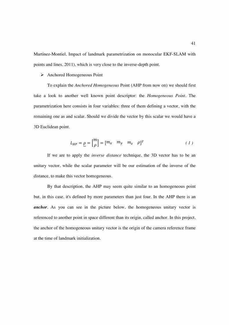
! Anchored Homogeneous Point

To explain the Anchored Homogeneous Point (AHP from now on) we should first

take a look to another well known point descriptor: the Homogeneous Point. The

parametrization here consists in four variables: three of them defining a vector, with the

remaining one as and scalar. Should we divide the vector by this scalar we would have a

3D Euclidean point.

!"# = % = &'% ( = )'* '+ ', %-. ( 1 )

If we are to apply the inverse distance technique, the 3D vector has to be an

unitary vector, while the scalar parameter will be our estimation of the inverse of the

distance, to make this vector homogeneous.

By that description, the AHP may seem quite similar to an homogeneous point

but, in this case, it's defined by more parameters than just four. In the AHP there is an

anchor. As you can see in the picture below, the homogeneous unitary vector is

referenced to another point in space different than its origin, called anchor. In this project,

the anchor of the homogeneous unitary vector is the origin of the camera reference frame

at the time of landmark initialization.

42

Figure 12 - Homogeneous Anchored Point (AHP)

And so, the AHP parametrization is defined by seven variables, three to define the

anchor, and the remaining four to define the homogeneous unitary vector.

!/"# = 012'%

3 = )42 52 62 '* '+ ', %-. ( 2 )

! Adaptation of the AHP to key-frame based SLAM

However, the previous definition, which was designed to operate in EKF-

SLAM, is only valid if the homogeneous unitary vector is defined in the world reference.

In key-frame-based systems, the anchor exists in the problem representation as one of the

keyframes, and it is convenient to used to avoid redundancy. As the point is called

homogeneous "anchor" point, we can assume the unitary vector is expressed in the

camera reference. The camera reference, which acts as the anchor frame, can be

computed from the composition of the robot frame in world reference (thus the key-frame

43

at the time of landmark initialization), with the camera frame in robot reference.

Therefore, our landmark parametrization would look like this:

!/"# = ) 7 9 : ; 9 :

7 : < ; : <

' = %-. ( 3 )

where [ 7 9 : ; 9 : ] are position and orientation quaternion of the robot, at the time of

initialization, in world frame, and are encoded in the corresponding key-frame;

[ 7 : < ; : <

] are position and orientation of the camera in robot frame, and constitute the

extrinsic sensor parameters, which we consider constant and known; cm is a vector

defining the line of sight to the landmark expressed in camera frame; and ρ is the inverse-

distance parameter. The tuple [ ' = % ] constitutes the homogeneous vector in the

anchor (i.e. camera) frame, while [ 7 9 : ; 9 : 7 : < ; : <

] defines the anchor frame.

This way, the anchor is correctly defined, while using the inverse distance

technique for landmark parametrization.

44

Chapter 6

Implementation in WOLF

Two algorithms were developed implementing the WOLF structure. As the

specifications of the project are a requirement for both of these algorithms, they have

many similarities. Both have images in which to extract features, provided by a camera

sensor. However, they are ultimately defined by how they compute the residual in the

Constraint class: Feature against Feature and Feature against Landmark.

• Feature against Feature

Figure 13 - Feature against Feature algorithm

45

The general procedure is virtually the same as explained in Chapter 4.4, which

makes sense, as we are only applying classes derived from the base ones in the WOLF

tree. Since this project uses a monocular camera to acquire images, analyzing them for

feature detection, there will be a Sensor Camera, a Capture Image, and a Feature Point

Image class, respectively. This algorithm also introduces the Processor Image Feature

and Constraint Epipolar classes, which will detect, track and make constraints from one

Feature to another.

• Feature against Landmark

Figure 14 - Feature to Landmark algorithm

46

Since the problem is the same for both algorithms, many similarities will appear

in their procedures, and in the classes used to solve the problem. For example, Sensor

Camera, Capture Image and Feature Point Image are also needed in this algorithm, as

the approach taken requires Features obtained from a monocular camera. Even the

Processor Image Landmark has many similar functionalities with the previous Processor.

The main difference, however, is that this algorithm uses the Landmark AHP class, that

defines a 3D point in the environment, to initialize Landmarks and to make constraints

against Features in the class Constraint AHP.

During this chapter, the main classes in both of those algorithms will be

explained, along with their main functionality, so that the procedure is properly

understood.

6.1. pinholeTools

The pinholeTools was originally a class made by Joan Solà in the RTSLAM

project, from LAAS. It has been adapted into WOLF. Its main purpose is to perform

projection of a 3D point into a 2D plane, as well as the inverse method called back-

projection.

The main functions of this class are explained below in pairs, as most of the class

contains a method and its inverse. The mathematic background of these functions is

explained in the appendix.

47

• projectPointToNormalizedPlane & backprojectPointFromNormalizedPlane

The projectPointToNormalizedPlane function performs the pinhole

canonical projection. When introduced a 3D point, returns a 2D point in a

normalized plane.

On the other side, the backprojectPointFromNormalizedPlane does the

inverse, a canonical backprojection. When given a 2D point in the image plane it

returns the 3D backprojected point. It must be specified a depth parameter, which

will correspond to the missing third dimension, which by default is 1.

• distortFactor

Using the formula of the distortion model, and the distortion parameters

introduced, returns the distort factor, so the point can be modified according with

the model. This function can also be used to compute the correctionFactor, which

is the inverse method.

• computeCorrectionModel

With the distortion parameters, which correspond to the distortion model,

the inverse parameters can be obtained to compute the distortion correction model.

• distortPoint & undistortPoint

In the distortPoint, using the distortFactor, this function will apply radial

distortion to a 2D point.

48

In the inverse function, undistortPoint, and with the correction parameters

obtained through distortFactor, the function will correct the distortion applied to a

2D point.

• pixellizePoint & depixellizePoint

pixellizePoint uses the intrinsic parameters of the camera to transform a

2D point into a pixel of the image, whereas in depixellizePoint, a pixel of an

image is transformed into a 2D point in a normalized plane.

• projectPoint & backprojectPoint

The projectPoint function projects a 3D point into a pinhole camera with

radial distortion. To do so, it computes the previous functions

projectPointToNormalizedPlane, distortPoint and pixellizePoint.

The backprojectPoint, as the inverse function, does the transformation in

the other direction. It backprojects a pixel from a pinhole camera with radial

distortion into a 3D point, correcting the distortion in the process.

• isInRoi & isInImage

Both of these functions check if a 2D point is in the designated region of

interest of an image, or in the image itself.

49

6.2. Sensor Camera

In the current project only one sensor will be used: a monocular camera.

Therefore the intrinsic and extrinsic parameters are introduced in the problem through the

derived class Sensor Camera. These intrinsic parameters consist in values of the inner

calculations made by the camera, used to successfully project any 3D point into the

image plain. There are also the distortion parameters, which are needed to calculate the

radial distortion the image may have, and their counterpart, the correction parameters,

used to correct a radially distorted image.

The extrinsic parameters describe the position and orientation the camera has in

relation to the robot, as these values are needed to perform changes of reference frames

absolutely essential to the process.

! Variables

int img_width_;

int img_height_;

Eigen::VectorXs distortion_;

Eigen::VectorXs correction_;

The class has to store the width and height of the image, as well as three main

parameters for the pinhole model: the intrinsic, distortion and correction parameters.

These values are stored because they need to be accessed when performing the

projections of points from 3D to 2D. The intrinsic parameters are actually stored in a

variable from the base class, as it was already planned to be there from the start.

50

! Constructor

SensorCamera::SensorCamera(const Eigen::VectorXs& _extrinsics, const IntrinsicsCamera*

_intrinsics_ptr) : SensorBase(SEN_CAMERA, "CAMERA", nullptr, nullptr, nullptr, 2), img_width_(_intrinsics_ptr->width), // img_height_(_intrinsics_ptr->height), // distortion_(_intrinsics_ptr->distortion), // correction_(distortion_.size()) // {

assert(_extrinsics.size()==7 && "Wrong intrinsics vector size. Should be 7 for 3D");

p_ptr_ = new StateBlock(_extrinsics.head(3));

o_ptr_ = new StateQuaternion(_extrinsics.tail(4));

intrinsic_ptr_ = new StateBlock(_intrinsics_ptr->pinhole_model);

}

The constructor receives intrinsic and extrinsic parameters, as expected. However,

as the input parameters are not in the usual State Block form, some of the variables have

to be assigned later. This is the case of the position and orientation, that are sent in the

form of an Eigen vector (extrinsic parameters), and have to be split in order to be

assigned correctly. Note that the orientation is stored as a State Quaternion, a class very

similar to a State Block which specializes in quaternions.

6.3. Capture Image

Capture Image is a derived class which stores image raw data. In this project,

such data is acquired by the Sensor Camera class.

! Variables

cv::Mat image_;

cv::Mat descriptors_;

std::vector<cv::KeyPoint> keypoints_;

51

This class stores the image in matrix form, with keypoints and descriptors defined

in the appropriate OpenCV format, so they can be used with other OpenCV functions

with ease.

6.4. Feature Point Image

The class Feature Point Image is derived from the Feature Base class. It has all

the functionality of that class while also implementing all the necessary functions and

variables to store the information of a point in 2D space.

! Variables

cv::KeyPoint keypoint_;

cv::Mat descriptor_;

bool is_known_;

• cv::Keypoint keypoint_

In the explanation of the base class it was mentioned that it needed a

measurement, which was designed as an Eigen vector of 2 dimensions. The

tracker used in this project already uses a specific element for that purpose, called

cv::keypoint. Moreover, most of the OpenCV functions in relation with vision use

it, so it made sense to maintain it in detriment of the Eigen vector to store point

data.

52

• cv::Mat descriptor_

As was already mentioned in Chapter 5.2.1, a point must have a descriptor

associated with it. It is indispensable if we are to compare the point, and to track it,

so it must be stored as well.

• bool is_known_

The purpose of this flag is to know if the tracked feature is a "new" feature

or a "known" one. More information about this feature in the implementation of

both Processor classes.

! Constructor

This class has two practical constructors (in reality it has more for debugging

purposes), each one is used in one of the two Processors explained in this project. The

first constructor is mainly used by the Processor Image Feature class, which uses

Features to compare other Features.

53

FeaturePointImage(const cv::KeyPoint& _keypoint,

const cv::Mat& _descriptor, bool _is_known) :

FeatureBase(FEATURE_POINT_IMAGE, "POINT IMAGE", Eigen::Vector2s::Zero(),

Eigen::Matrix2s::Identity()),

keypoint_(_keypoint),

descriptor_(_descriptor)

{

measurement_(0) = Scalar(_keypoint.pt.x);

measurement_(1) = Scalar(_keypoint.pt.y);

is_known_=_is_known;

}

The input parameters of this constructor are the three main variables previously

explained: the point information, the descriptor associated with that point, and a boolean

variable which identifies the feature as a "know" or "new" feature.

The main values are stored in the proper variables of the derived class, and the

pertinent information is send to the parent class in its own constructor. Notice that the

values sent in the base constructor are void of meaning, only to assign the proper value of

the keypoint in the measurement later, as that assignation could not be done in the

constructor line.

The second constructor is mainly used by the Processor Image Landmark class:

54

FeaturePointImage(const cv::KeyPoint& _keypoint,

const cv::Mat& _descriptor, const Eigen::Matrix2s& _meas_covariance) :

FeatureBase(FEATURE_POINT_IMAGE, "POINT IMAGE",

Eigen::Vector2s::Zero(), _meas_covariance),

keypoint_(_keypoint), descriptor_(_descriptor)

{

measurement_(0) = Scalar(_keypoint.pt.x);

measurement_(1) = Scalar(_keypoint.pt.y);

}

As it can be seen, the constructor is similar to the previous one. There are two

differences, however. First, the variable is_known is not included. The Processor uses

Landmarks, and a whole different approach is needed to operate with the Features, so it is

no longer necessary to know if the feature is "known" or "new". Moreover, the input

parameters of the constructor have included the measure covariance, which is properly

sent to the parent class, and is needed to calculate a solution of this problem.

6.5. Landmark AHP

The main function of this class is to store Landmarks using the "Anchored

Homogeneous Point (AHP)" parametrization (explained in chapter 5.3) and all auxiliary

variables it may need.

! Variables

cv::Mat cv_descriptor_;

FrameBase* anchor_frame_;

SensorBase* anchor_sensor_;

As it can be seen, there is not even one variable in this class to store the point (or,

in this case, the homogeneous unitary vector). The information arrives as an input

variable, but since it's a derived class it is sent to the Landmark Base class, as there are

55

means to store the value there (seen in Chapter 4.2.2.1). Instead, the three variables are

used to keep data that the base class can't store, as its related on how the point is

described.

When a Landmark is created the descriptor of the Feature is stored. That way,

when we perform the tracking of said Landmark, we will have the original descriptor in

which it was found, providing helpful information in deciding whether the Feature found

resembles the Landmark projection or not.

Of course, if we are to implement the AHP parametrization, the anchor

information must be preserved to successfully describe the point. With that in mind, we

store the Frame in which the Landmark was created, as it’s a necessary variable to

compute both the position and orientation of said Landmark. Another important variable

is the Sensor Base pointer, who will provide the intrinsic and extrinsic parameters of the

Sensor, essential in the computation of the residual in the Constraint class.

! Constructor

LandmarkAHP::LandmarkAHP(Eigen::Vector4s _position_homogeneous,

FrameBase* _anchor_frame,

SensorBase* _anchor_sensor,

cv::Mat _2D_descriptor) :

LandmarkBase(LANDMARK_AHP, "AHP", new StateHomogeneous3D(_position_homogeneous)),

cv_descriptor_(_2D_descriptor.clone()),

anchor_frame_(_anchor_frame),

anchor_sensor_(_anchor_sensor)

{

}

The input parameters are the expected ones: the homogeneous vector, the Frame

with the position and orientation, and the Sensor frame. All the assignations are also

56

expected, with one exception: WOLF has taken into account the possibility of having a

3D homogeneous vector, so if given a four vector with the correct values all the

necessary steps of conversion (so that the solver can understand that it's not an ordinary

State Block) will be handled automatically.

6.6. Constraint AHP

This Constraint AHP class calculates the residual error between a Feature and a

Landmark, with the particularization that the Landmark is defined as an "Anchored

Homogeneous Point". Therefore, we will be comparing the projection of a Landmark in a

2D plane against its measurement.

This class is derived from Constraint Sparse, which at the same time is a derived

class of Constraint Base. The Sparse class contains the operations needed to aid when

solving a sparse non-linear optimization problem such as this.

! Variables

Eigen::Vector4s intrinsics_;

Eigen::Vector3s extrinsics_p_;

Eigen::Vector4s extrinsics_o_;

Eigen::Vector3s anchor_p_;

Eigen::Vector4s anchor_o_;

The main variables of this class are just to store the parameters needed to

calculate the residual, such as the intrinsic and extrinsic parameters of the camera (which

are copied here only for speed reasons), and the position and orientation of the robot.

! Constructor

57

Before explaining the constructor of this class, we should take into account some

of the parameters needed by the Constraint Sparse.

class ConstraintImage : public ConstraintSparse<2, 3, 4, 3, 4, 4>

When creating the class, we must specify a numerical set of parameters to the

Sparse class. The first of the values is the size of the residual that is going to be

calculated. Since we will be comparing the projection of a Landmark and a measurement

on an image plane, the residual will have a size of two.

The rest of the input parameters also correspond to the sizes of the elements the

solver must take into account when solving the problem. In this particular problem, these

parameters correspond to the position and orientation of the current robot Frame, the

position and orientation of the anchor frame and the Landmark homogeneous unitary

vector. The positions of either the camera and the robot have a size of 3, and their

orientations have 4 (as they are quaternions). The homogeneous unitary vector, as seen in

Chapter 5.3, has also a size of 4.

58

static const unsigned int N_BLOCKS = 5;

ConstraintImage(FeatureBase* _ftr_ptr, FrameBase* _frame_ptr,

LandmarkAHP* _landmark_ptr, bool _apply_loss_function = false,

ConstraintStatus _status = CTR_ACTIVE) : ConstraintSparse<2, 3, 4, 3, 4, 4>(CTR_AHP, _landmark_ptr,

_apply_loss_function, _status, _frame_ptr->getPPtr(), _frame_ptr->getOPtr(),

_landmark_ptr->getAnchorFrame()->getPPtr(),

_landmark_ptr->getAnchorFrame()->getOPtr(),

_landmark_ptr->getPPtr()),

intrinsics_(_ftr_ptr->getCapturePtr()->getSensorPtr()->getIntrinsicPtr()-

>getVector()), extrinsics_p_(_ftr_ptr->getCapturePtr()->getSensorPPtr()->getVector()), extrinsics_o_(_ftr_ptr->getCapturePtr()->getSensorOPtr()->getVector()), anchor_p_(_landmark_ptr->getAnchorFrame()->getPPtr()->getVector()), anchor_o_(_landmark_ptr->getAnchorFrame()->getOPtr()->getVector()), {

setType("AHP"); }

The N_BLOCKS parameter is specifying the number of blocks what will be used

in the optimization. These blocks will be modified during the iteration process of the

solver, while it is trying to obtain the optimal state. Therefore, they must correspond to

defining variables in this problem. When calling for the Constraint Sparse class, it

requires the size of some parameters. Except for the first one (as it's the size of the

residual), the others correspond to the dimensions of the five blocks explained before.

These values have to be sent to the Constraint Sparse in the same order as they

were defined and must correspond with the numerical value specified. The class also

stores for itself these values, as it will need them to compute the residual.

! Functions

59

The main function of this class is the one that computes the residual.

template<typename T>

inline bool ConstraintImage::operator ()(const T* const _p_robot,

const T* const _o_robot,

const T* const _p_anchor,

const T* const _o_anchor,

const T* const _p_lmk,

T* _residuals) const

This function will be automatically called by the solver when it so requires, and

the input parameters are the blocks defined in the constructor, plus the residual. It is

important to note that this function is templatized, as the solver needs to use a type of unit

called Jet to perform the automatic calculation of the Jacobian matrices.

The mathematics performed in this function require to change the Landmark from

the camera reference it was originally created to the new one (in which the Constraint is

being made). These operations involve four chained frame transforms: camera-to-anchor-

frame, anchor-frame-to-world, world-to-current-frame, and current-frame-to-camera; plus

a projection onto image plane, plus a comparison against the measured point. They are

too extensive to be explained here, so they will be added in the appendix.

After the change of reference from the anchor camera position to the current

camera position, we have a vector referenced in the correct camera sensor. We must, then,

project that resulting vector with the intrinsic matrix K.

> = ? ∗ ! ="##$%& %$' =()$#( ( 4 )

And dividing the first two components of the homogeneous vector with the last

one we obtain the projection of the Landmark.

60

> = >(0; 1)>(2) ( 5 )

Then, with the value of the measurement contained within the Feature above the

Constraint, and the square root information of the measurement (computed when creating

the Feature), we obtain the residual.

01234>56 = (> − 8159>01_'152>01'1;9) ∗ 2;09_0<<9_3;8<0'593<; ( 6 )

This is computed for every Constraint, in multiple iterations, by the solver. The

code in this function has to be as optimized as possible to avoid overloading the

computational time here.

6.7. Processor Tracker

Before explaining the two derived Processor classes in this project we have to

present another class first, as those two classes will inherit the majority of the functions

from this one.

The Processor Tracker was developed by the WOLF team and is a derived class

from Processor Base. The most important function in this class is the one that introduces

a basic methodology to track elements that will be applied in even more derived classes,

called process.

! Incremental Tracker

The algorithm behind that function implements an incremental tracker, which is

a typical tracker for images. To do so it makes use of frames and keyframes. The

61

objective is to be able to successfully follow a Feature in one keyframe through different

frames. At one moment in time it is decided to create a new keyframe and new Features

are found, along with the ones that were successfully tracked, repeating the process.

Figure 15 - Incremental tracker example

As shown in the Figure above, the Features are tracked in respect with a

keyframe. As new Captures come, the Features are searched in them. In the Figure, the

algorithm dictates that, below a certain number of Features tracked, a new keyframe is to

62

be made, so new Features are found in that frame. Now, with the new keyframe, the

tracking process starts again.

! Process function

To implement the incremental tracker we will make use of the following

variables.

CaptureBase* origin_ptr_; ///< Pointer to the origin of the tracker. CaptureBase* last_ptr_; ///< Pointer to the last tracked capture. CaptureBase* incoming_ptr_; ///< Pointer to the incoming capture being processed.

It's important to remember that the Frame class must have a Capture hanging

from them. To ease computational cost it is more efficient just storing the class that

contains the visual data instead of the Frame.

The keyframe that serves as the origin for the tracking will be represented in the

origin Capture, and the frame in which we will search for Features in the incoming

Capture. The Features found, however, won't be compared with the ones in origin, but

instead to the ones in the last Capture. This last Capture corresponds to the last non-

keyframe analyzed aside from the one we are currently working on.

63

Figure 16 - Features found in the incoming Capture successfully tracked in last

The Figure above explains more visually how the three elements work. The role

of the origin Capture is obvious, as the next Captures have track their Features with

origin's. The purpose of the last Capture, however, is not so obvious: It is the last Capture

in which some of the origin's Features are still being tracked. Between last and origin

there may be a numerous amount of other Frames previously analyzed, and the Features

tracked in last must also have been found in each and every one of these other Frames.

Therefore, any Features we wish to compare found in the new incoming Capture have to

be compared with last, which indirectly compares them with origin.

The whole algorithm can described in pseudo code with these simple functions.

process(CaptureBase* incoming) • processKnown () • if voteForKeyFrame ()

o processNew () o makeKeyFrame () o reset ()

• else o advance ()

64

The function will analyze the incoming image in processKnown and then will

decide through the voteForKeyFrame function if it's time to make a new keyframe or not.

In case it is not necessary, the advance function will continue with the algorithm:

the incoming Capture will now be the last Capture, with all the tracked Features it has

found. The previous last Capture will be eliminated, because since there is a new Capture

with more temporally advanced successful tracks, it's not needed anymore. And a new

iteration will begin, repeating the process.

In case it is decided to make a new keyframe, using the function processNew

more Features will be found and added to the last Capture, and these particular subset of

the Features will also be tracked in the incoming. After that, as the last Capture is the last

Frame in which the requirements to track are still valid, it will be made into a keyframe.

The reset function will put all the Frames in their right order: the last Capture will be the

new origin, and incoming will now take the place of last. The process will begin anew,

expecting a new incoming Capture.

The processKnownFeatures and processNewFeatures, as the main functions of

process, should behave like this in a derived class, though it may vary depending on the

implementation.

65

processKnownFeatures () • track () • establishConstraints ()

processNewFeatures ()

• if detectNewFeatures () o track() o if usesLandmarks ()

" initLandmarks () " establishConstraints ()

As you can see, this pseudo code of both functions is in concordance with the

whole process algorithm. Each of these functions will have to be implemented in derived

classes, so the exact details on how they operate will be done it their respective class.

! Sidenote

Besides the process function, the class also implements the functions preProcess

and postProcess. Their purpose is to perform certain tasks that either can't be done in the

main function of the class or have to be done before or after.

6.8. Processor Tracker Feature

The Processor Tracker Feature class was developed by the WOLF team and is

derived from Processor Tracker. It will implement the functions inside process to

establish constraints Feature to Feature. This class details the methodology used for five

of the main functions in process. At the same time, it defines functions as "pure virtual",

which must be implemented in yet another derived class.

66

! processKnown

The main purpose of this function is to successfully track Features against other

Features inside the incoming Capture. To do this, it implements two pure virtual

functions that will be applied in a derived class, called trackFeatures and

correctFeatureDrift.

• trackFeatures

As the name implies, it will analyze the incoming Capture for

Features and later it will compare them with the Features in last, to track

them.

• correctFeatureDrift

Even if the track is successful, we are comparing based only on

the difference between the incoming and last Features. That difference is

not great, or else the Feature wouldn't be tracked, but in successive

iterations it can become a problem: the difference is still not enough to

break the tracking process, but the Features no longer resemble the origin

Features. That phenomenon is called drift.

The purpose of this function is to prevent the tracks from drifting.

Once there is a successful tracked Feature (in the previous function

trackFeatures) it will be compared again, not with last but instead against

origin. If the difference between them is low, the track has not a large drift

67

and it's still a viable Feature. If it's not, in hopes of correcting the drift, a

new search will begin only for that specific Feature. However, instead of

looking for the last Feature, the algorithm will search the origin Feature.

That way it may find a Feature that is a better match. In case no better

Feature is found, the Feature is discarded.

! processNew

The objective of this function is to populate the Capture with new Features. Later,

these Features must be found and tracked in the next Capture. To do that, the function

will use these two pure virtual functions, to be implemented in derived classes.

• detectNewFeatures

The main objective is to populate the last Capture with Features.

To do that, it will make use of one of the keypoint detectors implemented,

such as ORB or BRISK. Moreover, to search more efficiently the whole

image, this function will make use of the Active Search grid (explained in

Chapter 5.2.2).

• trackFeatures

Once detectNewFeatures has found the new Features, we will

make use of trackFeatures once more. As before, it will implement an

algorithm to search the correspondent incoming Features and compare

them with the ones found in last in the previous step. As it is not possible

68

for drift to happen in just one iteration, the correctFeatureDrift function is

not needed.

The new Features obtained through this method will be appended in the list of the

previously known Features, successfully populating the keyframe with already tracked

Features.

! establishConstraints

The purpose of the establishConstraints function is to create constraints between

the last and origin. To do so, it uses the function createConstraint with two different

Features (as the tracker compares Features against Features) to properly create it. And,

since it's a pure virtual function, it must be implemented in a derived class.

inline void ProcessorTrackerFeature::establishConstraints() {

for (auto match : matches_origin_from_last_) match.first->addConstraint(createConstraint(match.first, match.second.feature_ptr_)); }

! advance & reset

The advance and reset functions have quite a similar functionality in the code:

both of them actualize the values of the Captures, although they can't be operational at

the same time because one is meant to be used when making a new keyframe and the

other for any other case.

69

The voteForKeyFrame function decides whether or not to make a new keyframe.

If the decision is negative, the advance function is triggered. It means that the Features in

incoming have been tracked successfully, and that information must be stored so that the

next iteration will compare its Features against those. Therefore, the incoming will now

occupy the last Capture place, and the previous last will be erased (as the important

information is now on the new last).

If the decision to create a keyframe is affirmative, it will do so using the last

Capture. Since the reset function is triggered by that event, the last Capture will now

become origin. Likewise, the previous incoming Capture will move on to be the last. In

the next iteration a new incoming Capture will arrive and the process will repeat.

Figure 17 - Advance and Reset functionality illustration

70

! General overview

As most of the functions explained here are to be implemented in yet another

derived class, here is a general overview of the elements included and explained in this

class, as well as those inherited from Processor Tracker.

! preProcess ! process

# processKnown o trackFeatures o correctFeatureDrift

# if voteForKeyFrame o processNew

• detectNewFeatures • trackFeatures

o makeKeyFrame o establishConstraints

• createConstraints o reset

# else o advance

! postProcess

6.9. Processor Image Feature

The Processor Image Feature class is a derived class from Processor Tracker

Feature. It implements all the functions defined in the upper class to perform the tracking

of Features against Features.

As you can see, while there are functions from previous (and upper) Processor

classes, some of them are unique of this derived class, to aid with the tasks that the more

important functions have to do.

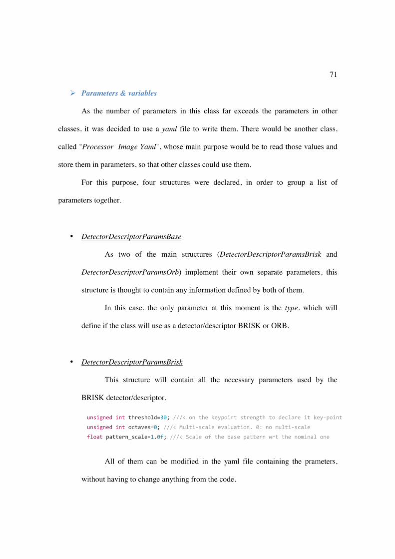
71

! Parameters & variables

As the number of parameters in this class far exceeds the parameters in other

classes, it was decided to use a yaml file to write them. There would be another class,

called "Processor Image Yaml", whose main purpose would be to read those values and

store them in parameters, so that other classes could use them.

For this purpose, four structures were declared, in order to group a list of

parameters together.

• DetectorDescriptorParamsBase

As two of the main structures (DetectorDescriptorParamsBrisk and

DetectorDescriptorParamsOrb) implement their own separate parameters, this

structure is thought to contain any information defined by both of them.

In this case, the only parameter at this moment is the type, which will

define if the class will use as a detector/descriptor BRISK or ORB.

• DetectorDescriptorParamsBrisk

This structure will contain all the necessary parameters used by the

BRISK detector/descriptor.

unsigned int threshold=30; ///< on the keypoint strength to declare it key-point

unsigned int octaves=0; ///< Multi-scale evaluation. 0: no multi-scale

float pattern_scale=1.0f; ///< Scale of the base pattern wrt the nominal one

All of them can be modified in the yaml file containing the prameters,

without having to change anything from the code.

72

• DetectorDescriptorParamsOrb

For the ORB detector/descriptor there is also a structure to store the

parameters.

unsigned int nfeatures=500; ///< Nbr of features to extract

float scaleFactor=1.2f; ///< Scale factor between two consecutive scales of the image

pyramid

unsigned int nlevels=1;///< Number of levels in the pyramid. Default: 8

unsigned int edgeThreshold=4; ///< ? //Default: 31

unsigned int firstLevel=0;

unsigned int WTA_K=2;

unsigned int scoreType=cv::ORB::HARRIS_SCORE; ///< Type of score to rank the detected

points

unsigned int patchSize=31;

This parameters can be modified as well, just changing the value in the

correspondent yaml file.

• ProcessorParamsImage

The three previous structures were made to contain parameters of the

detector/decriptor, while this one has to store all the necessary parameters used in

the execution of the class.

It has four substructures to keep the data organized:

73

# Image o width

///< Width of the image o height

///< Height of the image # Matcher

o min_normalized_score ///< [0 .. 1] Minimum score to decide if a Feature found matches another

o similarity_norm ///< Norm used to measure the distance between descriptors

o roi_width ///< Width of the ROI used in tracking

o roi_height ///< Height of the ROI used in tracking

# Active Search o grid_width

///< Cells per horizontal dimension of the image o grid_height

///< Cells per vertical dimension of the image o separation

///< Distance between the border of the cell and the border of the associated ROI # Algorithm

o max_new_features ///< Max. number of features to be detected in one frame

o min_features_for_keyframe ///< Min. number of features required to vote for a keyframe

! Helper functions

• detect

Since the image has to be analyzed for Features a large number of times in

each iteration, the detect function is very handy. Independently of the selected

detector/descriptor the function analyzes only a small region of interest of the

image provided, storing the keypoints of all the Features and their descriptors.

74

To analyze the image we make use of the keypoint detectors and

descriptors provided by the OpenCV library, as well as some of the functions

provided by it. At the time to write this project, the detectors/descriptors available

are ORB and BRISK. Moreover, we use the OpenCV functions detect and

compute to detect the keypoints in the image and to describe them, respectively.

The selection of the region of interest (ROI) must be decided outside this

function, as its only purpose is to analyze whatever it is told to analyze. Another

of the "helper functions", adaptRoi, will be the one to assure that the ROI has the

necessary requirements to work in the best conditions.

• match

The main purpose of this function is to compare descriptors. There is

usually a "target" and many "candidates", and the OpenCV function match will

compare their binary descriptors using the Hamming distance method and return

the candidate whose descriptor is more similar to the target. Once we obtain the

result it is normalized.

;<0'563614 2=<01 = >392 <8 4388101;=1 >19?11; 950@19 5;4 =5;434591>392 <8 9ℎ1 412=0379<0 ( 7 )

• adaptRoi

This function is actually formed by another two: trimRoi and inflateRoi.

One of the other helper functions, detect, is given a region of interest (ROI) of the

75

image to search for Features. adaptRoi makes sure that this ROI has the right

requirements to be used.

In Chapter 5.2.1 it was explained how, to detect and describe a keypoint,

some pixels around said keypoint were needed. This means that the

detector/descriptor needs some space to operate with a point, and in this situation

any ROI analyzed would have a small zone in which no keypoints are detected, as

the ROI doesn't have enough space to detect or describe it. Therefore, inflateRoi

expands the boundaries of the ROI just the pixels the detector and descriptor

needs, to assure the ROI is completely search and kept as small as possible. After

that, the function trimRoi asserts that the given ROI is within the image: If the

ROI has some parts of it outside the image, it trims them so there are no errors

when searching in that space.

At last, the modified ROI is assigned to the image, so that the detect

function can work more efficiently.

! Main functions

• preProcess

The main purpose of the function is to have a tool to implement some

functionality external to process, as well as to initialize variables before it starts.

This is the case of the Active Search, for instance, as it has to be refreshed at

every iteration so that the grid has a random offset each time.

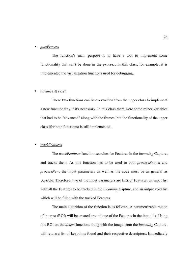
76

• postProcess

The function's main purpose is to have a tool to implement some

functionality that can't be done in the process. In this class, for example, it is

implemented the visualization functions used for debugging.

• advance & reset

These two functions can be overwritten from the upper class to implement

a new functionality if it's necessary. In this class there were some minor variables

that had to be "advanced" along with the frames, but the functionality of the upper

class (for both functions) is still implemented.

• trackFeatures

The trackFeatures function searches for Features in the incoming Capture,

and tracks them. As this function has to be used in both processKnown and

processNew, the input parameters as well as the code must be as general as

possible. Therefore, two of the input parameters are lists of Features: an input list

with all the Features to be tracked in the incoming Capture, and an output void list

which will be filled with the tracked Features.

The main algorithm of the function is as follows: A parametrizable region

of interest (ROI) will be created around one of the Features in the input list. Using

this ROI on the detect function, along with the image from the incoming Capture,

will return a list of keypoints found and their respective descriptors. Immediately

77

after we call the match function to compare the newfound keypoints descriptors

against the descriptor of the Feature we want to track, which will return a

normalized score.

If the returned score is lower than the parametrizable value of

"min_normalized_score", the Feature has not been tracked. On the other hand, if

the value is higher it means that is was successfully tracked. The candidate

keypoint is then converted to a Feature object and added to the output list of

Features.

This process is done for all the Features in the input list of Features. When

there are no more elements, the function returns the number of successfully

tracked Features.

• correctFeatureDrift

As previously stated in Processor Tracker Feature, this functions tries to

correct the phenomenon called drift. The first step to correct the drift is to detect

it, so the descriptor of an incoming Feature and the origin one are compared in the

match function, which returns a normalized score.

If the returned score is higher than a parametrizable score we can assume

there is no drift. If the score is lower, however, the drift must be corrected.

To do that correction we will search for the Feature once more in the

incoming Capture. The methodology is almost the same as the one in

trackFeatures. This time, however, we will use the origin Feature descriptor to

78

compare instead of last's. If the normalized score returned by the match function

is higher than the "minimum score", the new keypoint is converted into a Feature,

taking the place of the old incoming Feature (which had drift). If the normalizes

score is lower, the correction doesn't take place.

• voteForKeyFrame

This function is the one that decides if we should create a new keyframe of

not. Many different algorithms can be applied here to decide, varying from simple

to really complex.

In this project it was decided to count the number of tracked Features: if

the value is lower than a certain parameter, a new keyframe will be created in the

last Frame (as it was the last to meet the requirements specified here).


The main goal of this function is to populate the image with Features. As a

parameter of the class, "max_new_features" can limit the number of iterations

made, and thus the number of new Features found.

The algorithm uses the Active Search grid, as it will provide a random,

void of any Features, region of interest (ROI) to search. With that ROI we will

use the detect function to find new keypoints and their associated descriptors.

OpenCV has an internal score when using keypoint descriptors (such as

ORB or BRISK), and the function retainBest will analyze the list of keypoints and

79

select the one with the highest score. This selected keypoint is, among those in the

list, the most identifiable of all, and it's more likely to be tracked successfully in

the next frames so it is converted into a Feature and added to the list of Features

in the last Capture.

After that, the Active Search is informed that we found a Feature in that

cell. If that was not the case, because the detect function is unable to find any

keypoint in the ROI, the Active Search is also properly informed.

• createConstraint

inline ConstraintBase* ProcessorImage::createConstraint(FeatureBase* _feature_ptr,

FeatureBase* _feature_other_ptr)

{

ConstraintEpipolar* const_epipolar_ptr = new ConstraintEpipolar(_feature_ptr,

_feature_other_ptr);

return const_epipolar_ptr;

}

This function is rather simple, as the only operation to be done is to create

a Constraint element. In the case of the Processor Image Feature class, the one

used will be the Constraint Epipolar.

At the moment of writing this project, this Constraint has not been

developed yet. The whole algorithm concerning the Feature against Feature

method works, but as it doesn't have a Constraint class that can compute a

residual, the optimizer can't solve anything.

80

6.10. Processor Tracker Landmark

The Processor Tracker Landmark was developed by the WOLF team, and is a

derived class from Processor Tracker. It implements the necessary steps so that the

function process can establish constraints Feature against Landmark. This class details

the methodology used for five of the main functions in process. At the same time, it

defines functions as "pure virtual", which must be implemented in yet another derived

class.

! processKnown

The main purpose of this function is to project the Landmarks in the environment

and successfully find them inside the incoming Capture. To do this, it implements a pure

virtual function that will be applied in a derived class, called findLandmarks.

• findLandmarks

In general aspects, findLandmarks is quite similar to the

trackFeatures function (used in Processor Image Feature), as both try to

find a correlation between a Feature and something else. In this case we

are now searching for the relation between a Feature and a Landmark. The

function will have to implement a projection of the Landmark, as a

landmark is a 3D element in the space and can't be compared trivially with

a 2D Feature.

81

The other difference with trackFeatures is that all this methodology is

done only on the incoming Capture. The Landmarks are always there, so just

projecting and searching for them in that Capture is enough.

! processNew

The objective of this function is to populate with Features the Capture that is

going to become the new keyframe. Later, these Features will be used to create

Landmarks. To do that, the function will use three pure virtual functions, to be

implemented in derived classes.


The main objective is to populate the Capture with Features. To

accomplish that, the function will make use of one of the keypoint

detectors implemented, such as ORB or BRISK. Moreover, to search more

efficiently the whole image, this function will make use of the Active

Search grid (explained in Chapter 5.2.2).

• createNewLandmarks

Once we have these new Features, this function will create the

Landmarks. To do that, it will make use of the pure virtual function

createLandmark, that must be implemented in a derived class.

82

• findLandmarks

Once createNewLandmarks has created this new set of Landmarks,

we will make use this function once more. This way it is assured that the

new created Landmarks are found, and a Constraint can be established.

Once findLandmarks ends, we will have a list of Features that correspond to

projections of Landmarks, and it will be appended to the current list.

! establishConstraints

The purpose of the establishConstraints function is to create constraints between

the last and origin frames. To do that, however, uses the function createConstraint with a

Feature and a Landmark to properly create it. And, since it's a pure virtual function, it

must be implemented in a derived class.

inline void ProcessorTrackerLandmark::establishConstraints()

{

for (auto last_feature : *(last_ptr_->getFeatureListPtr()))

last_feature->addConstraint(createConstraint(last_feature,

matches_landmark_from_last_[last_feature]->landmark_ptr_));

}

! advance & reset

The Processor Tracker Landmark doesn't use the last Capture except for when

creating a Constraint. Taking that into account, the only operation these two functions do

is move the list of Features in incoming to last.

83

! General overview

As most of the functions explained here are to be implemented in yet another derived

class, here is a general overview of the elements included in this class, as well as those

inherited from the Processor Tracker.

! preProcess ! process

# processKnow o findLandmarks

# if voteForKeyFrame o processNew

• detectNewFeatures • createNewLandmarks

o createLandmark • findLandmarks

o makeKeyFrame o establishConstraints

• createConstraints o reset

# else o advance

! postProcess

6.11. Processor Image Landmark

The Processor Image Landmark is a derived class from Processor Tracker

Landmark. It implements all the functions defined in the upper class to perform the

tracking of Features against Landmarks.

As you can see, while there are functions from previous (and upper) Processor

classes, some of them are unique of this derived class, to aid with the tasks that the more

important functions have to do.

84

! Parameters & variables

As the parameters and variables of this class are exactly the same as the

ones used in the Processor Image Feature, to read about them go to Chapter 6.9.

! Helper functions

• detect, match & adaptRoi

These three functions are exactly the same as the ones in the Processor

Image Feature. To know about their functionality, go to Chapter 6.9.

• rotationMatrix

This function generates a rotation matrix from a given quaternion. The

rotation matrix associated with a quaternion is as follows.

BC;D = E;'F + ;*F − ;+F − ;,F 2H;*;+ − ;';,I 2H;*;, + ;';+I

2H;*;+ + ;';,I ;'F − ;*F + ;+F − ;,F 2H;+;, − ;';*I2H;*;, − ;';+I 2H;+;, + ;';*I ;'F − ;*F − ;+F + ;,F

J ( 8 )

• changeOfReferenceFrame

It contains the operations needed to find the translation vector and rotation

matrix which will perform a change in reference from the previous camera

position to the current one. The formulas behind this function can be found in the

appendix.

85

• getLandmarkInReference

Implements the change in reference from the previous camera position to

the current one with the translation and rotation obtained through

changeOfReferenceFrame. Moreover, it transforms the homogeneous vector (now

on the correct camera reference frame) into the Euclidean coordinates. The

formulas behind this function can be found in the appendix.

! Main functions

• preProcess & postProcess

These two functions are already explained in the class Processor Image

Feature, as they are exactly the same as the ones used there. For more information

about their functionality, go to Chapter 6.9.

• advance & reset

These two functions can be overwritten from the upper class to implement

a new functionality if it's necessary. In this class there were some minor variables

that had to be "advanced" along with the frames, but the functionality of the upper

class (for both of the functions) is still implemented.

• findLandmarks

The main purpose of this function is to find the projection of all the

Landmarks visible by the camera. For that we will project the Landmarks, and

86

around the projected pixel a search for a Feature with a similar descriptor will

begin.

The function has only two main input parameter: the list of all the

Landmarks and a void Feature list. The following algorithm has to be

implemented for each one of the Landmarks in the list.

First of all, the analyzed Landmark is described as an homogeneous

unitary vector with an anchor, as explained in Chapter 5.3. That means that the

Landmark is described in another camera position and orientation than the one

currently using. If it's not referenced to the current camera position, the projection

of the Landmark will return an erroneous point. Therefore, before projecting the

Landmark, we must use the two helper functions changeOfReferenceFrame and

getLandmarkInReference. The first function makes all the necessary operations to

find the translation vector and rotation matrix needed to change from the previous

camera to the current one, and the second function implements that operation and

transforms the homogeneous vector into the Euclidean coordinates. The

mathematics behind these two functions are explained in the appendix.

After that, the 3D point obtained is ready to be projected into the plane of

the camera. We make use of the pinholeTools class to do the projection, with the

functions projectPointToNormalizedPlane and pixelizePoint, which make the

projection to the plane and transform that 2D point into a pixel of the image,

respectively. Then the isInImage function (also from the pinholeTools class)

analyzes the pixel to check if the projection of the Landmark at this moment is

87

still within the image. The output of this function checks whether this Landmark

can or can't be seen from this camera position. In case it can't, the function ends

and the Landmark is not found.

A parametrizable region of interest (ROI) is created around the resultant

pixel. Using the ROI on the detect function will return a list of keypoints found

and their descriptors. Then, we call the match function to compare the newfound

keypoints descriptors against the descriptor of the analyzed Landmark, which will

return a normalized score.

If the returned score is lower than the parametrizable variable

"min_normalized_score", that would mean that the keypoint found doesn't match

with the projected Landmark. On the other hand, if the value is higher it means

that the Landmark was successfully found. The candidate keypoint is then

converted to a Feature object and added to the output list of Features.

• voteForKeyFrame & detectNewFeatures

These two functions are exactly the same as the ones in Processor Image

Freature. To know more about these two functions, go to Chapter 6.9.

• createLandmark

The Landmark class that is going to be used in this problem is called

"Landmark AHP", as the "Anchored Homogeneous Point" is the most adequate

point description for this case.

88

Since we have to create a Landmark from a Feature, the first step must be

to make this Feature homogeneous. We add another dimension to it with an

unitary value to do so. After that, we must obtain the intrinsic matrix (K) stored in

the Sensor data and apply this operation to obtain a direction vector with

reference in the camera:

' = = ?KL ∗ > ( 9 )

If this direction vector is normalized we will obtain the same direction

vector but in unitary form.

' = = ' =‖ ' = ‖ ( 10 )

As it is explained in Chapter 5.3, the Landmark AHP class needs an

homogeneous unitary vector, and the complete position and orientation of its

anchor. We have the necessary unitary vector, so it must be converted into an

homogeneous one adding another dimension. As we are using the "inverse

distance" technique, the value of this new dimension will be that of the inverse of

distance to that point. Since we don't know where will that point be, the

"distance" parameter is just a prior estimation. Nonetheless, the value has to be

the inverse of that distance estimation.

ℎ<'<@1;1<>2 >;39505 !1=9<0 = N ' = L, ' = F, ' = P, 143295;=1Q ( 11 )

For the position and orientation of the anchor it's only needed to get the

last Frame, as the Frame in which the Landmark is created is the anchor of said

Landmark.

89

Lastly, the Landmark AHP class also needs the descriptor of the Feature

the Landmark is based on, as it's needed if we want to compare the descriptors

when using the findLandmarks function.

• createConstraint

The createConstraint function is rather simple, as it's used only to create

the derived class Constraint AHP. This class needs a Feature and the

correspondent Landmark to establish a constraint between the two. It is also

needed the last Frame as it's the anchor of that Landmark.

90

Chapter 7

Results

After explaining WOLF and the derived classes created for this project, we should

take a look at the performance when tested. The most important results are summarized

here, in an orderly fashion, up to the moment of writing this project.

! Keypoint detector

As we have seen though the project, two detector/descriptor systems are used to

find features: BRISK and ORB. The first tests were done by BRISK and it was the

selected detector until the tracker was implemented, being used with still images, video

footage and real cameras. The main issue encountered with that detector is that, for

reasons yet unknown, BRISK couldn't maintain the tracks of the features. It certainly

detected keypoints, but when a new capture came in it could find most of the previous

keypoints. All those found keypoints were twitching in a really close space, as if they

were dancing around the true keypoint position (for example, a well defined corner).

It was then decided to implement the ORB detector, and the difference was

remarkable. The keypoints didn't twitch around like in BRISK and they were almost

fixed to the same salient point in the image, which improved the performance of the

tracker. From that moment on, the default detector and descriptor used in the project

became ORB. Of course, the BRISK implementation is still available in the code.

91

! Tracker - Feature against Feature

The Processor Image Feature has all the necessary classes from the WOLF tree

already defined to aide it to track and match the features found. However, there is one

class that, due to time restraints could not be implemented, prevents the whole system to

obtain a solution to the problem: it lacks a Constraint class to compute the residual.

Without a residual the solver can't iterate and find an optimal state, therefore the problem

can't be solved. Nonetheless, all the functionality in the system works well and

consistently. The tracker, despite using ORB as it main detector/descriptor, and being far

better than the BRISK alternative, is not as robust as we would like it to be. At the

moment of writing this project a solution for this issue has not yet been found, mostly due

to time restrictions, although one of the guesses indicates that it's possible that it returns a

high number of erroneously matched tracks, which would hinder the performance of the

other parts of the system.

! Tracker - Feature against Landmark

On the other hand, the class Processor Image Landmark has the complete WOLF

tree to apply the methodology explained in the previous chapter. In Figure 18 we can

visualize a test done with a real camera. The Landmark projections are represented in big

red dots, while the keypoint candidates to be compared to that projection are represented

as little cyan dots. The square around the Landmark projection is the region of interest

(ROI) in which to search those candidates.

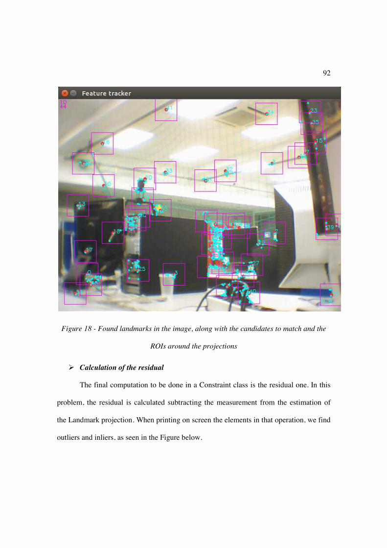
92

Figure 18 - Found landmarks in the image, along with the candidates to match and the

ROIs around the projections

! Calculation of the residual

The final computation to be done in a Constraint class is the residual one. In this

problem, the residual is calculated subtracting the measurement from the estimation of

the Landmark projection. When printing on screen the elements in that operation, we find

outliers and inliers, as seen in the Figure below.

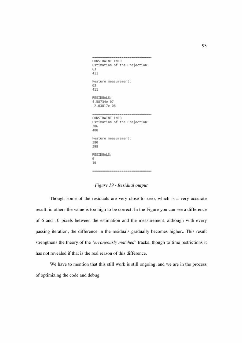
93

Figure 19 - Residual output

Though some of the residuals are very close to zero, which is a very accurate

result, in others the value is too high to be correct. In the Figure you can see a difference

of 6 and 10 pixels between the estimation and the measurement, although with every

passing iteration, the difference in the residuals gradually becomes higher.. This result

strengthens the theory of the "erroneously matched" tracks, though to time restrictions it

has not revealed if that is the real reason of this difference.

We have to mention that this still work is still ongoing, and we are in the process

of optimizing the code and debug.

94

! Solver convergence

To solve the problem, the optimizer must modify the positions and orientations of

the elements included in the problem in such a way as to minimize the sum of all

residuals . At each one of these iterations, the optimizer calls the Constraints, and asks for

the residual.

Figure 20 - Ceres Solver Summary print

When the solver is called, it tries to compute a solution through iteration, as seen

in Figure 20. When looking at the difference between the "successful steps" and the

95

"unsuccessful steps", it is patent that something is not going as it should. This in

enhanced with the "cost" values, as the initial and final values are almost the same.

The solver iterates and converges into a solution, but the amount of unsuccessful

movements towards the optimal state keeps the solution stale. And the Figure only shows

one of the first operations with the solver: As time goes on in the problem, the optimizer

is completely unsuccessful and doesn't converge.

One explanation for this could be the high value of the residuals. To even the

values of all the residuals is the method in which the solver will arrive to the optimal

solution. With such high values of the residuals, it is possible that, no matter what

direction the solver makes a step, some of the residuals are always going to have high

outputs. In this case, the solver would almost always take an "unsuccessful step", thus not

converging as gradually more residuals have to be dealt with.

! ROS implementation

Last, but not least, we must talk about the Robot Operating System (ROS)

implementation with WOLF. The structure in which ROS operates is really compatible

with WOLF. In that regard, a ROS node was created to run an early version of the

"Feature against Feature" tracker implementation.

96

Figure 21 - Test of the WOLF node in ROS

The camera sensor already had a ROS node, so the connection between the two

nodes was fairly simple. Features are obtained and, although this implementation runs

with BRISK, some tracks are successfully found. However, as the Processor Image

Feature evolved, this did not. As of now, this ROS node is deprecated.

97

Chapter 8

Project Management

8.1. Planning

The project can be split in three identifiable parts: the Research, in which

information about the project is gathered, the Implementation, part in which the code is

developed, and the Documentation, reserved for the making of this document. The

general overview of the project is as follows.

Figure 22 - General overview of the project

Seeing the duration of each one of the parts it is clear that majority of the effort in

this project went to the Implementation part. If we look with a little more detail in each of

these parts, we find this:

Figure 23 - Detailed overview of the project

98

Applying the detailed overview over a Gantt diagram, we can visualize the

complete planning with ease.

Figure 24 - Gantt diagram of the project

The majority of the project was used in the Implementation part, specially to

create both of the Processor classes. Since they are the ones giving the orders to the other

classes it is to be expected. The Constraint AHP also required some time to developed as

it computes the residual, which is crucial to the development to the project.

8.2. Costs

The costs can be divided in two groups: Human Resources and Hardware

Resources.

• Human Resources

Assuming 8 hours of work per day, with a varying cost per hour depending on the

task, as the amount of effort is different too. Using the number of days from Figure 22,

we can calculate the human resources cost.

99

Days Hours Price Total Cost

Research 31 248 14 € 3472 €

Implementation 110 880 18 € 15840 €

Documentation 16 128 12 € 1536 €

Total 157 1256 20848 €

The total cost of the human resources amounts to 20848 €.

• Hardware Resources

Only a computer has been used in this project, a desktop computer from IRI. The

UAV in which the testing has to be done is not taken into account as it has not been used

in the span of the current project.

• HP desktop computer with an Intel Core i5-650 Processor at 3.20 GHz with 8Gb

RAM memory (≈ 500 €)

Assuming a 3 year life for the computer, the hardware cost is computed like this:

R504?501 =<29 = 500 €3 51502 ∗ 12 '<;9ℎ2 5150V ∗ 22 4552

'<;9ℎV ∗ 8 ℎ<>02 455V

≅ 0,08 €/ℎ<>0

Therefore, if we multiply by the number of hours, we will obtain the total hardware cost.

Z<956 R504?501 [<29 = 0,08 €ℎ<>0 ∗ 1256 ℎ<>02 = 100,48 €

100

The total cost of the project is expressed as the sum of both costs:

Z<956 [<29 = R504?501 012. + R>'5; 012. = 20848 € + 100,48 €

= 20948,48 €

101

Chapter 9

Conclusions

The goal of the current project is to develop a system that is able to compute the

position and orientation of an UAV via camera sensors with the WOLF library.

We have managed to implement a system that is able to extract data from an input

camera sensor and analyze it with a keypoint detector. When it tries to compute its own

position and orientation using visual odometry and SLAM techniques, as of the moment

of writing this project, it's unsuccessful. We are in the process of debugging and

optimizing our code for this objective to be achieved.

The WOLF library was used to perform this task, contributing in its development

as well by creating the classes that would implement the strategy and algorithms needed

for the project. Moreover, two different approaches have been made to solve the problem:

tracking the features found in an image against other features, or against environmental

landmarks.

The main objective of the project has been almost completed, and further testing

will assure the success of this goal.

102

Chapter 10

Future Work

There are still a lot of improvements to be made to the project. As it is now, the

optimizer can't compute the optimal state as it doesn't converge, so a solution to this

problem is one of the first things that have to be done.

It has been mentioned that the current project can be used with an inertial model

to measure rotational velocities and translational accelerations, and it could be an

interesting approach to test these features with an unmanned aerial vehicle (UAV) in

simulated and real environments.

Another nice improvement could be to implement an outlier rejection. If a point is

far too distant from the others, it increases the error of the whole process. Those points

have to be dealt with and an outlier rejection method like RANSAC (Random Sample

Consensus) would be a good option. The alternative would be applying the loss function,

a functionality already incorporated in the code, although RANSAC would perform

better.

ROS is a really nice tool to use alongside with WOLF. A test of a WOLF node in

ROS was developed, but it was done in early stages of the project, so there is a lot of

room for further testing.

103

Bibliography

Andrew J. Davison. 2003. Real-Time Simultaneous Localisation and Mapping with a Single Camera. In Proceedings of the Ninth IEEE International Conference on Computer Vision - Volume 2 (ICCV '03), Vol. 2. IEEE Computer Society, Washington, DC, USA, 1403-. IRI. (n.d.). Wolf - Image branch. Retrieved 9 5, 2016, from https://github.com/IRI-MobileRobotics/wolf/tree/image IRI. (n.d.). WOLF - Windowed Localization Frames. Retrieved 9 5, 2016, from https://github.com/IRI-MobileRobotics/wolf KONOLIGE, Kurt ; AGRAWAL, Motilal ; SOLÀ, Joan ; KANEKO, Makoto (Bearb.) ; NAKAMURA, Yoshihiko (Bearb.): Large-Scale Visual Odometry for Rough Terrain.. 66. In: ISRR : SPRINGER, 2007 (Springer Tracts in Advanced Robotics). - ISBN 978-3-642-14742-5, S. 201-212 Stefan Leutenegger, Margarita Chli, and Roland Y. Siegwart. 2011. BRISK: Binary Robust invariant scalable keypoints. In Proceedings of the 2011 International Conference on Computer Vision (ICCV '11). IEEE Computer Society, Washington, DC, USA, 2548-2555 Montiel, J., Civera, J., & Davison, A. J.. Unified Inverse Depth Parametrization for Monocular SLAM. In: Proceedings of Robotics: Science and Systems (2006) Mostofi, N., Elhabiby, M. M., & El-Sheimy, N. (2014). Indoor localization and mapping using camera and inertial measurement unit (IMU). Position, Location and Navigation Symposium - PLANS 2014, 2014 IEEE/ION (pp. 1329 - 1335). IEEE. OpenCV. (n.d.). OpenCV docs. Retrieved 9 5, 2016, from http://docs.opencv.org/2.4/modules/features2d/doc/feature_detection_and_description.html#orb ROS. (n.d.). ROS: The Robot Operating System. Retrieved from http://www.ros.org/ Roussillon, C., Gonzalez, A., Solà, J., Codol, J.-M., Mansard, N., Lacroix, S., et al. (2011). RT-SLAM: a generic and real-time visual SLAM. Ethan Rublee, Vincent Rabaud, Kurt Konolige, and Gary Bradski. 2011. ORB: An efficient alternative to SIFT or SURF. In Proceedings of the 2011 International Conference on Computer Vision (ICCV '11). IEEE Computer Society, Washington, DC, USA, 2564-2571.

104

J. Solà. Course on SLAM. Technical Report IRI-TR-16-04, Institut de Robòtica i Informàtica Industrial, CSIC-UPC, 2016. J. Solà. Quaternion kinematics for the error-state Kalman filter. Technical Report IRI-TR-16-02, Institut de Robòtica i Informàtica Industrial, CSIC-UPC, 2016. Solà, J. Towards Visual Localization, Mapping and Moving Objects Tracking by a Mobile Robot: a Geometric and Probabilistic Approach. Ph.D. thesis, Institut National Polytechnique de Toulouse ( 2007) Solà, J., Vidal-Calleja, T., Civera, J., & Martinez-Montiel, J. M. (2011). Impact of landmark parametrization on monocular EKF-SLAM with points and lines. International Journal of Computer Vision , 339-368. Strasdat, H., Montiel, J. M., & Davison, A. J. (2010). Real-time monocular SLAM: Why filter? Robotics and Automation (ICRA), 2010 IEEE International Conference on (pp. 2657 - 2664). IEEE. Wang, C., Wang, T., Liang, J., Chen, Y., Zhang, Y., & Wang, C. (2012). Monocular visual SLAM for small UAVs in GPS-denied environments. Robotics and Biomimetics (ROBIO), 2012 IEEE International Conference on (pp. 896 - 901). IEEE.

105

Appendix

1. changeOfReferenceFrame

The function is trying to implement a change of reference frame from a

"previous" camera frame to the "current" one. The mathematics to do that can be

summarized as:

`!

1 %V a

=== bB Z

0 1cd=

==`

'1 %V a

d= ( 12 )

In which the index "cc" stands for "current camera", and "pc" stands for

"previous camera". The rotation and translation returned from this function are these two

values. However, to know to properly obtain them though calculations, we must redefine

the transformation in more detail, expressing it like this:

`!

1 %V a

=== bB Z

0 1c=#

==bB Z

0 1c9

=#bB Z

0 1cd#

9bB Z

0 1cd=

d#`

'1 %V a

d= ( 13 )

To transform the "previous camera" frame into the "current camera" frame, we

will have to pass through "previous robot", "world", "current robot" and "current

camera" frames. However, we don't have the transformations from "world" to "current

robot" and "current camera" as they are here, only the inverse. We will apply the

following transformation principle:

bB Z0 1c

e

/= bB. −B.Z

0 1 c/

e ( 14 )

106

With that in mind, the previous transformations now can be expressed as:

`!

1 %V a

=== bB. −B.Z

0 1 c==

=#bB. −B.Z

0 1 c=#

9bB Z

0 1cd#

9bB Z

0 1cd=

d#`

'1 %V a

d= ( 15 )

Operating with the matrices will lead to find the rotation and translation that go

from "previous camera" to "current camera" frame.

2. getLandmarkInReference

With the function changeOfReferenceFrame, we now have the values of the

translation vector and rotation matrix.

`!

1 %V a

=== bB Z

0 1cd=

==`

'1 %V a

d= ( 16 )

The purpose of this function is to apply the transformation to the unitary vector,

therefore:

! == = H Bd= == ∗ ' d= I + H Zd= == ∗ 1 %V I ( 17 )

And, after that, we obtain an Euclidean point doing this:

7 Pf = ! (0; 2)!(3)g ( 18 )

3. pinholeTools operations

The equations behind the functions of the pinholeTools are listed here. (Solà,

2007)

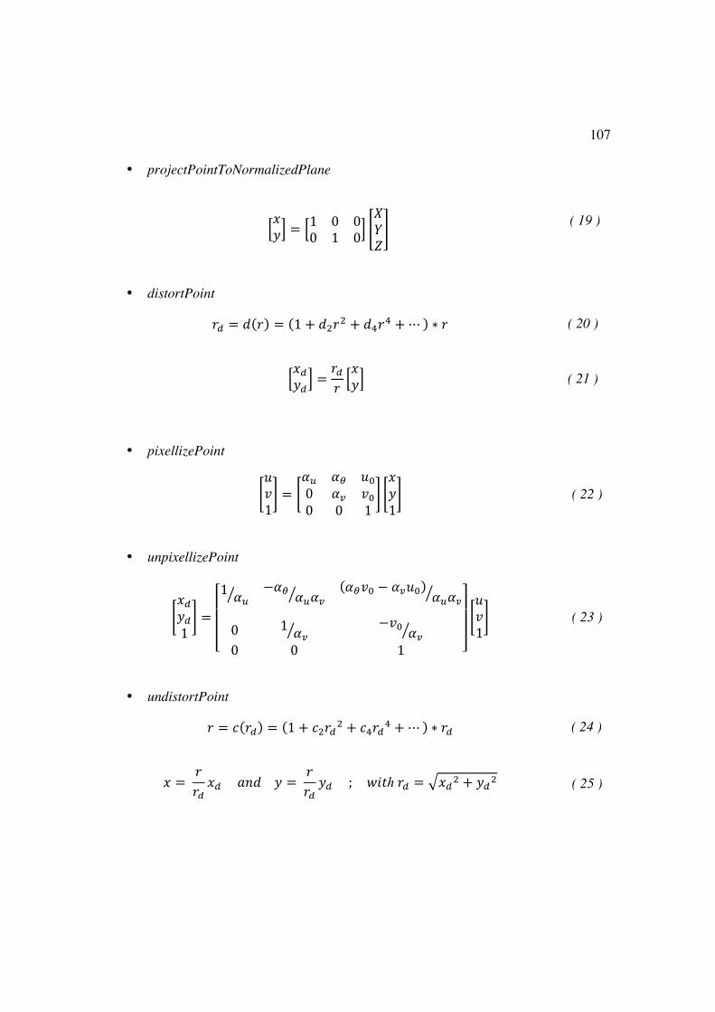
107

• projectPointToNormalizedPlane

&45( = &1 0 0

0 1 0( 0hij

3 ( 19 )

• distortPoint

0k = 4(0) = (1 + 4F0F + 4l0l + ⋯ ) ∗ 0 ( 20 )

&4k5k

( = 0k0 &4

5( ( 21 )

• pixellizePoint

n>!1

o = np" pq >r0 ps !r0 0 1

o n451

o ( 22 )

• unpixellizePoint

n4k5k1

o =

tuuuv1 p"V −pq p"psV (pq!r − ps>r) p"psV

0 1 psV −!r psV0 0 1 w

xxxy

n>!1

o ( 23 )

• undistortPoint

0 = =(0k) = (1 + =F0kF + =l0kl + ⋯ ) ∗ 0k ( 24 )

4 = 00k

4k 5;4 5 = 00k

5k ; ?39ℎ 0k = z4kF + 5k F ( 25 )

108

• backprojectPointFromNormalizedPlane

0hij

3 = 2 n451

o ( 26 )

4. WOLF code

The code used for every class, in both the .h and .cpp forms, would take a

considerable amount of space. On this event, it was decided not to include it directly, but

to put a reference to the github branch where it is stored. (IRI)

Implementation of a Visual SLAM System - Institut de … objective, which is the implementation of a...

Documents

Transcript of Implementation of a Visual SLAM System - Institut de … objective, which is the implementation of a...