Implementation of a multinomial logit model with …Implementation of a multinomial logit model with...

Implementation of a multinomial logit modelwith fixed effects

Klaus Pforr

Mannheim Centre for European Social Research (MZES)University of Mannheim

[email protected]

July 1, 2011,Ninth German Stata Users Group Meeting, Bamberg

Outline

Motivation

Statistical model

Implementation

First applications

Outlook

Motivation

Why mlogit?

▶ Fixed effect models available for continuous, binary andcount data dependent variables.

▶ Polytomous categorical dependent variables commonlyused in all fields of social sciences.

Why fixed effects?Counter omitted variable bias!

▶ With fixed effects models no assumptions about αinecessary.

▶ Random effects and pooled models basically assume nocorrelation of αi and Xit .

Statistical modelmlogit across time with unobserved heterogeneity

Pr(yit = j) =exp(αij + Xitβ

′j )

1 + ∑Jk=1,k ∕=B exp(αij + Xitβ

′k )

for j ∕= base outcome B

Pr(yit = B) =1

1 + ∑Jk=1,k ∕=B exp(αij + Xitβ

′k )

Solution by Chamberlain(1980)▶ ∑

Tit=1 yitj is sufficient statistic for αij

▶ Cond. probability model: Prob. of sequence yi1, . . . ,yiTi

cond. of "overall tendency" to each outcome j ∕=B.▶ αi disappeares!

Pr(yi ∣⋀

j ∕=B ∑Tit=1 yitj) =

∏Tit=1 ∏

Jj=1,j ∕=B exp(Xit β

′j )

yitj

∑di∈Δi((∏

Tit=1 ∏

Jj=1,j ∕=B exp(Xit β

′j )

ditj ))

withΔi = {(di1, . . . ,diTi )

′∣∀j = 1, . . . ,J, j ∕= B : ∑Tit=1 ditj = kij}.

Statistical model (cont.)

Δi is the set of all permutations of yi .

Example: Let yi=(1,2,3).Δi = {(1,2,3),(1,3,2),(2,1,3),(2,3,1),(3,1,2),(3,2,1)}.

Estimation with maximum-likelihood

The log. likelihood function:

lnL = ∑i

(∑j ∕=B

∑t

yitjXitβ′j − ln∑

Δi

exp ∑j ∕=B

∑t

ditjXitβ′j

)

Implementation: General layout

Top-level ado

▶ Syntax▶ Further preparation

Actual estimation with maximum likelihood▶ Iteration management & display of results via Stata ml▶ Log likelihood, gradient, Hessian with Mata evaluator

function

Implementation: Top-level ado"Outer shell"

▶ Standard parsing with syntax: varlist, group id, optionalbase outcome

▶ Missings: Standard listwise deletion via markout▶ Collinear Variables: Copied & adjusted _rmcoll from

mlogit▶ Matsize check: Copied & adjusted from clogit▶ Editing of equations for ml: Copied & adjusted from mlogit▶ Offending observations/groups, i.e. checks variance in

dep. & indep. var’s; copied & adjusted from clogit▶ Init. values: inspired by clogit▶ Remaining preparation for mata function:

▶ Globals for group id var., indep. var’s for ml evaluatorfunction

▶ Matrix out2eq: Mapping from outcome indices to outcomesvalues and equation indices.

Implementation: Maximum likelihood

"Interface": Stata ml

Putting equations in Stata’s ml terminology▶ Panel structure⇒ no likelihood defined at observation

level⇒ d-family method▶ Computation speed and accurary⇒ d2 method, i.e.

lnL,g,H have to be analytically derived▶ J-1 equations, i.e.

(y1, . . . ,yJ−1) = (y1, . . . ,yB−1,yB+1, . . . ,yJ)

▶ J-1 parameters θj = Xitβ′j ; not used, direct use of

(J−1)×M coefficients βjm

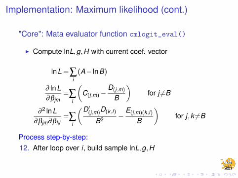
Implementation: Maximum likelihood (cont.)

"Core": Mata evaluator function cmlogit_eval()

▶ Compute lnL,g,H with current coef. vector

lnL =∑i

(A− lnB)

∂ lnL∂βjm

=∑i

(C(j ,m)−

D(j ,m)

B

)for j ∕=B

∂ 2 lnL∂βjm∂βkl

=∑i

(D′(j ,m)D(k ,l)

B2 −E(j ,m)(k ,l)

B

)for j ,k ∕=B

Process step-by-step:




lnL =∑i

(A− lnB)

∂ lnL∂βjm

=∑i

(C(j ,m)−

D(j ,m)

B

)for j ∕=B


=∑i

(D′(j ,m)D(k ,l)

B2 −E(j ,m)(k ,l)

B

)for j ,k ∕=B

Process step-by-step:1. Declare variables.




lnL =∑i

(A− lnB)

∂ lnL∂βjm

=∑i

(C(j ,m)−

D(j ,m)

B

)for j ∕=B


=∑i

(D′(j ,m)D(k ,l)

B2 −E(j ,m)(k ,l)

B

)for j ,k ∕=B

Process step-by-step:2. Get data, etc. from Stata.




lnL =∑i

(A− lnB)

∂ lnL∂βjm

=∑i

(C(j ,m)−

D(j ,m)

B

)for j ∕=B


=∑i

(D′(j ,m)D(k ,l)

B2 −E(j ,m)(k ,l)

B

)for j ,k ∕=B

Process step-by-step:3. Derive N,T ,J.




lnL =∑i

(A− lnB)

∂ lnL∂βjm

=∑i

(C(j ,m)−

D(j ,m)

B

)for j ∕=B


=∑i

(D′(j ,m)D(k ,l)

B2 −E(j ,m)(k ,l)

B

)for j ,k ∕=B

Process step-by-step:4. Loop over i using panelsetup




lnL =∑i

(A− lnB)

∂ lnL∂βjm

=∑i

(C(j ,m)−

D(j ,m)

B

)for j ∕=B


=∑i

(D′(j ,m)D(k ,l)

B2 −E(j ,m)(k ,l)

B

)for j ,k ∕=B

Process step-by-step:5. Compute A = ∑j ∕=B ∑t yitjXitβ

′j




lnL =∑i

(A− lnB)

∂ lnL∂βjm

=∑i

(C(j ,m)−

D(j ,m)

B

)for j ∕=B


=∑i

(D′(j ,m)D(k ,l)

B2 −E(j ,m)(k ,l)

B

)for j ,k ∕=B

Process step-by-step:6. At gradient-step (if (todo>0)), compute C(j ,m) = ∑t yitjxitm




lnL =∑i

(A− lnB)

∂ lnL∂βjm

=∑i

(C(j ,m)−

D(j ,m)

B

)for j ∕=B


=∑i

(D′(j ,m)D(k ,l)

B2 −E(j ,m)(k ,l)

B

)for j ,k ∕=B

Process step-by-step:7. Loop over Δi (permutations of yi ) using cvpermute




lnL =∑i

(A− lnB)

∂ lnL∂βjm

=∑i

(C(j ,m)−

D(j ,m)

B

)for j ∕=B


=∑i

(D′(j ,m)D(k ,l)

B2 −E(j ,m)(k ,l)

B

)for j ,k ∕=B

Process step-by-step:8. Add up B = ∑Δi

exp(∑j ∕=B ∑t ditjXitβ′j )




lnL =∑i

(A− lnB)

∂ lnL∂βjm

=∑i

(C(j ,m)−

D(j ,m)

B

)for j ∕=B


=∑i

(D′(j ,m)D(k ,l)

B2 −E(j ,m)(k ,l)

B

)for j ,k ∕=B

Process step-by-step:9. At gradient-step (if (todo>0)), add up

D(j ,m) = ∑Δi ∑t ditjxitm exp(∑j ∕=B ∑t ditjXitβ′j )




lnL =∑i

(A− lnB)

∂ lnL∂βjm

=∑i

(C(j ,m)−

D(j ,m)

B

)for j ∕=B


=∑i

(D′(j ,m)D(k ,l)

B2 −E(j ,m)(k ,l)

B

)for j ,k ∕=B

Process step-by-step:10. At Hessian-step (if (todo>1)), add up

E(j ,m)(k ,l) = ∑Δi ∑t ditjxitm ∑t ditkxitl exp(∑j ∕=B ∑t ditjXitβ′j )




lnL =∑i

(A− lnB)

∂ lnL∂βjm

=∑i

(C(j ,m)−

D(j ,m)

B

)for j ∕=B


=∑i

(D′(j ,m)D(k ,l)

B2 −E(j ,m)(k ,l)

B

)for j ,k ∕=B

Process step-by-step:11. After loop over Δi , build panel-wise lnLi ,gi ,Hi




lnL =∑i

(A− lnB)

∂ lnL∂βjm

=∑i

(C(j ,m)−

D(j ,m)

B

)for j ∕=B


=∑i

(D′(j ,m)D(k ,l)

B2 −E(j ,m)(k ,l)

B

)for j ,k ∕=B

Process step-by-step:12. After loop over i , build sample lnL,g,H




lnL =∑i

(A− lnB)

∂ lnL∂βjm

=∑i

(C(j ,m)−

D(j ,m)

B

)for j ∕=B


=∑i

(D′(j ,m)D(k ,l)

B2 −E(j ,m)(k ,l)

B

)for j ,k ∕=B

Process step-by-step:And that’s it! (with one ml-step)

First applications: How to use it

Syntaxfemlogit depvar indepvars, group(varlist) [baseoutcome(#)]

Data structure▶ Long panel-wise, condensed alternative-wise:

i t yit xit1 1 1 .51 2 2 .21 3 3 .92 1 1 .12 2 2 .32 3 1 .2▶ t not necessary.

Examples: Benchmark clogit

How precise and how fast is it?Comparison with clogit for J = 2.

▶ Data used:http://www.stata-press.com/data/r11/union.dta

▶ Relative difference of coefficients: 9.078e-16.▶ Speed: clogit: 2.42 sec., femlogit: 101.58 sec..

Examples: Simulated data

Performance with more alternativesSimulated data

▶ N=1000, T=5, J=5▶ Unobs. het. αij : over all i random draw (αi1, . . . ,αi5) from

uniform distribution over 4-simplex Δ4.▶ Error εitj : over all i and t, for each j indep. draws from

Gumbel-distribution (E(εitj) = γ,Var(εitj) = π/√

6).▶ Indep. variable: x correlated with α

▶ xit = uit + αi2,▶ uit drawn from uniform distribution.

▶ Coefficients β2 = 2,β3 = 3,β4 = 4,β5 = 5.

Examples: Simulated data (cont.)

▶ Utility Uitj : for each i and t

Uit1 =εit1

Uit2 =10αi2 + β2xit + εit2

...Uit5 =10αi5 + β5xit + εit5

▶ Dep. var.: yit = j with Uitj = maxk (Uitk )

Examples: Simulated data (cont.)

Results

informative observations: N=3405; speed: 20.83 sec.

Outlook

Things to do

▶ "tomorrow"▶ Document and publish

▶ in near future▶ Add standard options (if/in-able, ml-options, etc.)▶ Think about special postestimation▶ Robust estimates

▶ in far future▶ Intuitive Interpretation▶ Nested logit with fixed effects▶ Parametric serial correlation▶ Implementation of RE-Models & Hausman-Test

Thank you!

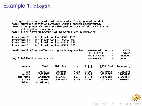
Example 1: clogit

Example 2: femlogit

Implementation of a multinomial logit model with …Implementation of a multinomial logit model with...

Documents

Transcript of Implementation of a multinomial logit model with …Implementation of a multinomial logit model with...