Implementation of a Hydraulic Power Take-Off for … D4.7 ISSN 1901-726X DCE Technical Report No....

Deliverable D4.7

ISSN 1901-726X DCE Technical Report No. 157

Implementation of a Hydraulic

Power Take-Off for wave energy applications

Francesco Ferri Peter Kracht

Department of Civil Engineering

DCE Technical Report No. 157

Implementation of a Hydraulic Power Take-Off for wave energy applications

by

Francesco Ferri Peter Kracht

May 2013

© Aalborg University

Aalborg University Department of Civil Engineering

Structural Design of Wave Energy Devices

Scientific Publications at the Department of Civil Engineering Technical Reports are published for timely dissemination of research results and scientific work carried out at the Department of Civil Engineering (DCE) at Aalborg University. This medium allows publication of more detailed explanations and results than typically allowed in scientific journals. Technical Memoranda are produced to enable the preliminary dissemination of scientific work by the personnel of the DCE where such release is deemed to be appropriate. Documents of this kind may be incomplete or temporary versions of papers—or part of continuing work. This should be kept in mind when references are given to publications of this kind. Contract Reports are produced to report scientific work carried out under contract. Publications of this kind contain confidential matter and are reserved for the sponsors and the DCE. Therefore, Contract Reports are generally not available for public circulation. Lecture Notes contain material produced by the lecturers at the DCE for educational purposes. This may be scientific notes, lecture books, example problems or manuals for laboratory work, or computer programs developed at the DCE. Theses are monograms or collections of papers published to report the scientific work carried out at the DCE to obtain a degree as either PhD or Doctor of Technology. The thesis is publicly available after the defence of the degree. Latest News is published to enable rapid communication of information about scientific work carried out at the DCE. This includes the status of research projects, developments in the laboratories, information about collaborative work and recent research results.

Published 2013 by Aalborg University Department of Civil Engineering Sohngaardsholmsvej 57, DK-9000 Aalborg, Denmark Printed in Aalborg at Aalborg University ISSN 1901-726X DCE Technical Report No. 157

Recent publications in the DCE Technical Report Series

ISSN 1901-726X DCE Technical Report No. 157

Contents

1 Objectives 4

2 Nomenclature 5

3 Introduction 8

4 Power Take-Off system (PTO) 10

4.1 General Aspects . . . . . . . . . . . . . . . . . . . . . . . . . . . . . . . . . . 10

4.2 Power take-off types . . . . . . . . . . . . . . . . . . . . . . . . . . . . . . . 10

4.2.1 Direct mechanical driven system . . . . . . . . . . . . . . . . . . . . . 10

4.2.2 Air/Water turbine system . . . . . . . . . . . . . . . . . . . . . . . . 11

4.2.3 Hydraulic system . . . . . . . . . . . . . . . . . . . . . . . . . . . . . 11

4.3 State of the art . . . . . . . . . . . . . . . . . . . . . . . . . . . . . . . . . . 12

4.3.1 Hydraulic PTO - Configuration 1 . . . . . . . . . . . . . . . . . . . . 12



4.3.4 Hydraulic PTO - Other configurations . . . . . . . . . . . . . . . . . 15

5 Model Implementation 17

5.1 WEC dynamical model . . . . . . . . . . . . . . . . . . . . . . . . . . . . . . 17

5.2 Hydraulic PTO model . . . . . . . . . . . . . . . . . . . . . . . . . . . . . . 21

6 Simulations 26

7 Results and Discussions 28

8 Conclusion 37

Appendices 40

A Wavestar: Hydrodynamic and hydrostatic parameters 40

B PTO length 42

2

C Simulink Model 43

C.1 Simulink Submodels: Floater . . . . . . . . . . . . . . . . . . . . . . . . . . . 43

C.2 Simulink Submodels: Hydraulic Piston . . . . . . . . . . . . . . . . . . . . . 44

C.3 Simulink Submodels: Check Valves Bridge Rectifier . . . . . . . . . . . . . . 45

C.4 Simulink Submodels: HP and LP accumulators . . . . . . . . . . . . . . . . 46

C.5 Simulink Submodels: Motor and Generator . . . . . . . . . . . . . . . . . . . 49

3

1 Objectives

The main purpose of the following work is to implement a hydraulic power take-off systemcoupled with the dynamic model of a wave energy converter. In this work the Wavestarconcept will be used without any losses of the general principle since the power take-offsub-model can be coupled with any device, if a relative motion between to body is available.The document will be divided mainly in six chapters. Chapter 3 gives a general definitionof the wave energy status and problems, Chapter 4 gives an overall description of a PTOsystem with a closer look into the hydraulic systems, Chapter 5 describes how the systemhas been modeled, implemented and coupled with the WEC dynamic model (Chapter 5),Chapter 6 gives an overview of the parameter used for the simulation, i.e. wave condition,numerical solver method, hydraulic parameters, etc. Chapter 7 and Chapter 8 are endingthe work showing results and giving some general conclusion of what have been simulated.

4

2 Nomenclature

A list of acronyms and symbols used through the document are reported below,Table 1.Beside every item a brief description is given.

Table 1: Acronyms and Symbols

Symbols and Acronyms Description

ACRONYMSWEC Wave Energy ConverterPTO Power Take-OffPEC Primary Energy CaptureOT Over ToppingOWC Oscillating Water ColumnHP High Pressure attributeLP Low Pressure attributeSISO Single-input single output systemFOPM First order process modelFC Frequency converterDoF Degree of FreedomFRF Frequency Responce Functionirf Impulse Responce FunctionOM Operation and Mantainance

SYMBOLSdf floater diameterM Mass MatrixI Moment of InertiaCG, [xG, yG, zG] Center of gravityCB, [xB, yB, zB] Center of buoyancySij Waterplane momentsω Frequency, [rad/s]η Surface elevation∆ Displaced volumeξi Body displacement i-th DoFδij Kroenecker delta function, 1 if i=j and 0 otherwiseφi Velocity potential for the 6 general modesφ0 Velocity potential for the incoming waveFrad(iω) Radiation force, frequency domainfrad(t) Radiation force, time domainFex(iω) Excitation force, frequency domain

Continued on next page

5

...continued from previous pageSymbols and Acronyms Description

fex(t) Excitation force, time domainFhy(iω) Hydrostatic force, frequency domainfhy(t) Hydrostatic force, time domainA(ω) Added Mass matrix, [6x6]B(ω) Radiation Damping matrix, [6x6]C Hydrostatic Stiffness matrix, [6x6]a∞ Added Mass matrix at infinite frequency, [6x6]Krad Memory Fluid kernel function or Radiation force irfKex Excitation force irflPTO(t) PTO Moment ArmFPTO PTO Feedback forceβ Fluid Bulk moduluspA/pB Actual Pressure at piston chamber A/BV 0A/V

0B Initial volume of fluid in piston chamber A/B

aA/aB Piston area chamber A/B sidex Piston Positionx0 Initial piston positionv Piston Velocityθ WEC angular displacement

θ̇ WEC angular velocity

θ̈ WEC angular accelerationθ0 Initial WEC angular displacementq(t) Unspecific flow rateqLPA /qLPB Fluid flow rate from LP reservoir to piston chamber A/BqHPA /qHPB Fluid flow rate from HP reservoir to piston chamber A/BAleak Check valve leakage areaAmax Maximum check valve passage areapcrack δP at which the check valve start to openpmax δP at which the check valve start to closeCD Check valve coefficient of dischargeρ Fluid densityqm Motor flow rateqHP/qLP HP/LP reservoir flow rateγ Ratio of gas heat capacities Cp/CvCp Heat capacity for constant pressureCv Heat capacity for constant volume

qrfHP/qrfLP Flow rate across the relief valve for HP/LP reservoir

Continued on next page

6

...continued from previous pageSymbols and Acronyms Description

pHP (t)/pLP (t) HP/LP accumlator instantaneous pressurepatm Axtmospheric pressureα Motor displacementn(t) Motor rotational speedτgen Generator time constantτm Motor time constantPel Power delivered to the gridPacc Power accumulated into the HP accumulatorPabs Power harvest from the floaterPwave Power carried by the incoming wave

7

3 Introduction

There are several challenges in converting energy from sea waves into electricity. At least,WECs need to deliver electricity in compliance with the grid code of the specific country andthey need to resist up to 20 years and extreme sea conditions. While, the last issue mainlyconcerns with structure and economic analysis, the former one deals with power take-off(PTO) system. For these reasons and others wave energy is still in a pre-commercializedstage even if the field started to develop itself from the 1970s, leaded by the oil crisis. Evenif more than 100 concepts have been patented in the last 20 years, and only few deviceshave reached the pre-commercial stage, there is not a leading technology yet. Apparently,among them, no one has proven a clear and continuous working time without exception.This scenario opens the door of a wide research field, which needs to define a new technologyor make the available devices suitable for the commercialization stage. As mentioned before,nowadays, a WEC should not only produce power and resist the rough environmental con-dition, but it is request to produce the power in compliance with the grid code. This meansto be able to produce energy and on top of it help the grid when it is necessary/request.This includes helping the grid to recover a fault, send reactive power to the grid when a bigmachine stops to work, etc. For these reasons in the last years more people started to talkabout both mechanical and electrical smoothing system. The first class includes flywheel,gas accumulator, etc. while in the second class we will start to talk about Power Electronics,or Frequency Converter system, that is the state of the art in wind energy.The primary interest of this work is the description of the governing equations and the nu-merical implementation of a mechanical smoothing system coupled with an hydraulic PTO.The simulation of a physical model can be especially helpful in gaining insights to the dy-namic behavior and interactions that are often not readily apparent from reading theory. Tobe useful, a model should be realistic and yet simple to understand and easy to manipulate;these are conflicting requirements since realistic model are seldom simple and vice-versa.Following, the first step to take is asking oneself which is the general scope of the underlingsystem, i.e. are the transients important or the model should represent a steady-state behav-ior?As it will be explained in the text, the work will trace transient dynamics of the mechanicalcomponents for the selected PTO system, while neglegting electrical transient behaviors.Why hydraulic system? There are at least three different reasons to justify the utilizationof this type of system within the wave energy field:

• The wave energy density is rather high and its content is carried at low frequency,which match the field of application of hydraulic systems, where slow motions andhigh moments are generally used.

• Hydraulic systems are well known and robust, which can reduce the OM cost.

8

• Hydraulic systems can be coupled with gas accumulator in order to smooth down theincident power fluctuations.

Furthermore, hydraulic systems can be assembled with components adapted from standardcommercial applications and are suitable for control implementation.

9

4 Power Take-Off system (PTO)

4.1 General Aspects

In the following a short introduction of the available PTO systems for wave energy convertersis given followed by a specific description of the hydraulic systems. The PTO system can bedefined as the chain of processes that transform the available energy at the activated body,at the reservoir, at the air chamber, etc. into electricity to be delivered to the grid. Dueto the scattered distribution of WEC concepts a sharp classification of the available PTOsystems is not feasible, but mainly three different classes of PTO type are used in the waveenergy filed:

• Direct mechanical driven system

• Air/Water turbine system

• Hydraulic System

All of them receive high forces (up to MN) with long period (from 1-20 s) while the deliveredelectricity needs to fulfill the requested grid quality. Furthermore, it is important to bearin mind the severe environment conditions where the device is situated (i.e. high salinity,distance from land, high load in storm condition, water spray, slamming load, etc.). Theseparameters define constrains, which the PTO system need to satisfy.

4.2 Power take-off types

It is possible to define a common scheme for all the three general PTO classes, where theavailable energy, either kinetic or potential, is transferred from the so-called primary energycapture (PEC) object (i.e. activated body, water reservoir, etc.) into the generator, in paral-lel with a control scheme, and a storage system (if needed). Following a general descriptionof the three PTO classes cited.

4.2.1 Direct mechanical driven system

This type of PTO system directly links the generator to the PEC via mechanical connectors.Mechanical connectors can be a simple mooring line, a gearbox, a pulley, a belt, and theyare normally used in point absorber WECs. The electricity can be generated using a linearor rotating generator. In both cases the velocity fluctuations need to be compensated usingstorage and a frequency converter system. For this type of PTO the available storage systemcan be battery or electrochemical cells, ultracapacitor and flywheel. All of them have pros

10

and cons, i.e. battery has relative high energy density but short life time and not envi-ronmental friendly, while ultracapacitor has longer life horizon but higher prize. The mostcommon example of point absorber using direct mechanical driver are the Uppsala PointAbsorber and the ”L10” Buoy, both using a linear generator driven by the relative velocitybetween the active body and a reference body, which could be bottom fixed or a reactionplate.

4.2.2 Air/Water turbine system

This type of PTO transforms the energy stored in a fluid with high potential energy intomechanical energy, using a water or air turbine. When the process fluid is water, normallythe PTO is coupled with an OT WEC, where the water is collected in a floating/fixed-elevated basin using a profiled ramp, i.e. Wave Dragon and SSG. Collected water at higherquote it then funnels into a low-head turbine, i.e. Kaplan or Propeller type, and discharged.Valves are used to control the flux across the turbines. Typical available head for this typeof application is ranging from few meters to half a meter, in function of the basin water level,sea state, etc. Each turbine is coupled with a rotating generator, which should be able towork at variable speed. In this system both the basin and the number of turbine are usedto smooth out the produced electricity.When the process fluid is air, then the PTO is coupled with OWC WEC, where a pressuregradient across an air turbine is transformed into mechanical energy, i.e. Limpet and Picoplant, Oceanlinx floating structure. Since the air chamber works as high pressure side for halfof the wave period and as low pressure side for the rest, a distributor, or rectifying systemis requested. Opposite to the water turbine where there are no new concepts, into the airturbine field, new turbine types have been developed in order to achieve higher performancewithin the wave energy field, i.e Wells turbines. Here the turbine is coupled with a highspeed rotating generator, which should be able to work at different speeds. In this type ofPTO the common way to smooth the power output is basically a combination of flywheeland frequency converter.

4.2.3 Hydraulic system

In this class of PTO a liquid vector is used to drive a rotating generator through the meanof a hydraulic motor. A hydraulic piston pressurizes the fluid, which can be either oilor water, and the potential energy is then delivered either to a hydraulic motor or waterturbine and transformed into mechanical energy; which is in turn exchanged to electricityinto the generator. This type of PTO fits the feature of the wave potential since is ableto handle high loads with long periods and translating the information into high frequencyand constant speed request by the generator side. Furthermore, it is quite a robust andwell known system. Hydraulic PTO can use or not use storage system, and in both cases

11

the frequency converter is present. The hydraulic piston is often a double acting cylinderand a valve loop, i.e. check valves, 4-way directional valves, etc. is used to rectify the flowthrough the hydraulic motor. This last can be a variable or fixed volume motor or a high-head impulse water turbine, i.e. Pelton type, directly coupled with a rotating generator. Acommon storage system for this kind of application is a gas/spring pressurized accumulator,which can already ensure a high smoothening effect. Some of the available PTO systemconfiguration will be described more in details in the following pages. The controllability ofthe system is affected by the selected configuration and not all the hydraulic PTO systemsare suitable for active control. Different hydraulic PTO system configurations are used invarious applications as, point absorbers (Wavestar, CPT, AquaBUOY, OPT, Wavebob),attenuators (Pelamis, Dexadevice) and terminators (Oyster).

4.3 State of the art

In this section the focus is given to a literature review about the hydraulic PTO systems.The literature concerning the hydraulic PTO is one of the most rich; especially in the lastdecades new model have been published using various hydraulic systems and model com-plexity. Due to the strong knowledge in this field in the recent year also physical model havebeen developed and tested, [1, 2, 3]. The most studied model present in literature is a hy-draulic PTO with double acting hydraulic cylinder and high and low pressure accumulator.An auxiliary accumulator is then used to control the system feeding back energy into thehydraulic cylinder if a control law is applied. Following, a reference list of the most recentworks dealing with this type of model is given [4, 5, 6, 7, 8, 9]. The fluid compressibilityis included in all of them, directly or in an artificial way, except for the work carried outby Falcao. A different approach is presented by Costello [10], and Kamizuru [11], where adirect driven hydraulic motor is used, in order to remove the accumulator and control theoutput through the generator. In addition to the cited works [12, 13, 14] investigated theimplementation of the optimal control strategy together with a hydraulic PTO system. Fromthe above, three different configurations are defined.

4.3.1 Hydraulic PTO - Configuration 1

Figure 4.1 shows the most used hydraulic PTO configuration. The bidirectional flow from/tothe hydraulic piston chambers, is rectified using both a 4-way directional valve and, morecommonly, a rectifying bridge based on 4-monodirectional (check) valves. The piston, thatis sketched in light gray on the draw’s left side, can have two bidirectional connection orfour monodirectional connection pipes. Downline of the rectification block, two lines calledlow ( LP ) and high ( HP ) pressure rams are connected to a hydraulic motor, which leada generator in turn. The red line represents the HP ram and the blue line the LP ram.Moreover, each of these two lines is connected to a gas reservoir used to smooth the residual

12

Figure 4.1: Power take-off: Configuration 1. The red identifies a high pressure ram, the bluea low pressure ram and the black both of them

pulsation coming from the rectifying bridge. This scheme is analogue to a simple diodebridge AC-DC converter, used in electronic. The motor will work only in quadrant two,which means it will sink energy only in one direction of rotation and it will not be able tofeed energy back. The definition of quadrant is somehow important to define four distinctareas of operation: two directions: clockwise (CW) and couterclockwise (CCW) and twomodes: acceleration and deceleration. The quadrants are defined in the torque/velocityplot. In quadrant one the system works as a motor in the CW direction, in quadrant twothe system works as generator in the CW direction, in quadrant three the system worksas motor in the CCW direction and in quadrant four the system works as generator in theCCW direction.The hydraulic PTO in configuration 1 can not be controlled unless one of the followingoption is added:

1. Inclusion of an extra HP reservoir with controllable IN/OUT port through a 2-way

13

valve. Reservoirs should be connected directly to the piston chamber rams, red dottedarea in Figure 4.1. The valves delay can affect the controller operation.

2. Control the flow passing through the motor with a controllable 2-way valve, which inturn controls the piston chamber pressure and therefore the feedback force of the PTOsystem. The inertia of the fluid can have a significan impact on the controller delay.

3. Control the flow passing through the motor adding a controllable by-pass parallel tothe motor between the HP and LP rams. The accumulated energy is dissipated, thatis causing a drop of performance.

The pro of this configuration is the usage of simple components, but the main drawback isthe low level of control achived.


Figure 4.2 represents a so called hydraulic transformer circuit scheme. As for the formercase the motor is connected to the double acting hydraulic piston and the flux is previouslyrectified via a rectifying bridge. The motor needs to work only in the second quadrant. Thehydraulic piston is decoupled from the generator side using a variable displacement pumpdirectly connected to the shaft of the hydraulic motor. This results in a constant pressureat the generator side and the liquid can flow in a conventional fixed displacement hydraulicmotor mechanically connected to a generator. Additionally, HP and LP accumulators linkedto the motor rams are used to smooth any residual pressure fluctuation. The pro of config-uration 3 is the absence of fluctuation in the produced electricity, but once more the maindrawback is the limited control capability. As in the previous case, the introduction of extracontrolled reservoirs can be used to increse the control aptitude of the system.


Figure 4.3 represents a variable speed scheme. The double acting hydraulic cylinder feedsdirectly the motor. As a consequence of the absence of a rectifying bridge and accumulatorsthe motor is running at varaible speed and in both direction CW and CCW. That beingso the motor needs to work at least in quadrant two and four. Furthermore, if the PTOsystem needs to feed energy in the floater than the full four quadrants operation is needed,i.e. reactive control scheme. A relif valve is used to protect the system from high pressurelevels. The pro of this system is the high controllability achived, but to avoid fluctuation inthe produced energy a frequency converter needs to be included.

14

Figure 4.2: Power take-off: Configuration 2. The red identifies a high pressure ram, the bluea low pressure ram and the black a swiching pressure ram

4.3.4 Hydraulic PTO - Other configurations

The reader needs to bear in mind that this is only a rough and brief summation of thealready implemented and published different concepts, and other strategy are likely to ariseor been published. Just to give some examples:

• Hydraulic piston with multiple pressure chamber

• Hydraulic system with manifold and multi-level pressure accumulators

• Closed Loop Power split system with direct driven motor operating with four quadrant,high pressure reservoir and a secondary hydraulic motor with one quadrant operation

The last two PTO system are depict in the work carried-out by Kamizuru et al. [3], whereit is possible to find a comparison between different PTO lay-out as a function of parame-ters such as controllability, limitation, adaptability, smoothness, etc (Table 4 of the above

15

Figure 4.3: Power take-off: Configuration 3. The black identifies a swiching pressure ram

reference).Once a simplified model is obtained the next step require the derivation of the governingequation and their implementation/solution using numerical methods, which will be dis-cussed in the next chapter.

16

5 Model Implementation

As introduced earlier the simulation of a physical model can be especially helpful in gaininginsights to the dynamic behavior and interactions that are often not readily apparent fromreading theory. In this chapter the governing equations which describe the WEC and thePTO dynamic are introduced.

5.1 WEC dynamical model

The solution of the wave-body interaction can be achived with different degree of refinement.In this case a general overview or what we can call steady-state solution is sough and for thispurpose the result of the Laplace equation can be searched in the form of velocity potentialfunction, after a linearization of the boundary condition. The basic assumptions are thereforerigid body, inviscid flow, zero curl of the velocity vector field and small oscillation aroundthe static equilibrium, which are going to restrict the results range of validity. The forceacting on the system are obtained from the integration of the dynamic pressure field actingon the body wetted surface, while the pressure field can be evaluated from the velocityfield obtained in turn from the velocity potential function which is solution of the Laplaceequation in the fluid domain. The solution is normally obtained by splitting the probleminto three different sub-problems:

• Hydrostatic problem

• Radiation problem: force induced by the motion of the body in otherwise still water

• Diffraction and Scattered problem: force induced by the wave filed with fixed structure

Holding the small amplitude assumption for incoming wave and body motion, it is possibleto use the superposition principle to describe a more realistic random process. Therefore,without loss of generality it is possible to analyze the body response in regular wave, givingthe chance to have a better understand of the dynamical behavior. When a regular waveis sent to the body, it will respond at the steady-state with the same frequency, while theamplitude of the response is defined by the particular geometry and applied constrains, foreach of the 6 canonical modes. As shown in Figure 5.1 for a single rigid body the motion isdescribed by three translations and three rotations relative to a global coordinate system.

Since the body response differs with the frequency it is somehow useful to define the differentcontributions as a frequency functions. Moreover, since the problem has been decomposedin three different linear sub-problems, each of those can be defined by a constant multiplied

17

Figure 5.1: Definition of the canonical six degree of freedoms for a rigid body in water

by the specific input, for each frequency. The three different term which compose the totalforce are included in, eq 1

F khy(iω) = (ρ∆−m)gδk2 + (mzG − ρ∆zB)gδk4 − (mxG − ρ∆xB)gδk6 −

6∑j=1

ckjΞj(ω)

F krad(iω) = −

6∑j=1

(−ω2Ξk(ω)Akj + iωΞk(ω)Bkj)

F kex(iω) = −ρ

∫∫SB

(φ0∂φk∂n− φk

∂φ0

∂n

)dS = Re{Amag{F k

ex}eiωt+phase{Fkex}}

(1)

Where, F khy is the hydrostatic force acting on mode k, i is the immaginary unit, ω is the

rotational frequency, ρ is the water density, ∆ is the volume variation, m is the mass of thesystem, g is the acceleration of gravity, δkj is the Kroeneker delta function, zG is the vertical

18

position of the center of gravity, zB is the vertical position of the center of buoyancy, xGis the horizontal position of the center of gravity, xB is the vertical position of the centerof buoyancy, ckj are the hydrostaic stiffness coefficients, F k

rad is the radiation force actingon mode k, Ξk is Fourier tranform of the body displacement in mode k, AkJ is the addedmass coefficient, Bkj is the radiation damping coefficient, F k

ex is the excitation force anctingon mode k, Sb is the wetted surface, φ0 is the velocity potential of the icoming wave, φk isthe velocity potential of the mode k, dS is the delta surface, A is the wave amplitude. Thehydrostatic stiffness matrix (C) is constant and defined as:

C =

0 0 0 0 0 00 ρgS33 0 0 0 00 0 0 0 0 00 0 0 ρgS33 + ρg∆yB −mgyG −g(ρ∆xB −mxG) 00 0 0 0 0 00 0 0 0 −g(ρ∆zB −mzG) ρgS11 + ρg∆yB −mgyG

In order to keep the definitions as general as possible all the available DoF of the system aretaken into account and therefore two index k and j running from 1 to 6 are used to keep traceof the different components; this consideration entails that the force vector will be composedby three force and three moment components, while the displacement by three translationand three rotation components. Taking the inverse Fourier transform of the above equationsthe different forces will be described as time functions, eq 2

fkhy(t) = (ρ∆−m)gδk2 + (mzG − ρ∆zB)gδk4 − (mxG − ρ∆xB)gδk6 −6∑j=1

cijξk(t)

fkrad(t) =

∫ t

0

Kkrad(t− τ) ξ̇k(τ) dτ

fkex(t) =

∫ t

−∞Kkex(t− τ) η(τ) dτ

(2)

Where, fkhy(t) is the hydrostatic force acting on mode k in time domain, ξk is the displacement

in mode k, fkrad(t) is the radiation force acting on mode k in time domain, Krad is the Kernelfunction of the radiation force, fkex(t) is the excitation force acting on mode k in time domain,Kex is the Kernel function of the excitation force and η is the surface elevation at the centerof gravity of the floating body. Following, the displacement vector can be assessed solvingthe Newtons second law, where the system inertia is balanced by the summation of the forcesacting on the system, eq. 3:

Fk =6∑j=1

M−1kj ξ̈k (3)

19

Where Fk is the summation of the forces acting on the body for the mode k and M is themass matrix defined by a 6x6 matrix :

M = [mkj] =

m 0 0 0 mzG −myG0 m 0 −mzG 0 mxG0 0 m myG −mxG 00 −mzG myG I11 I12 I13

mzG 0 −mxG I21 I22 I23−myG mxG 0 I31 I32 I33

Where, Ilm is the moment of inertia coefficient.Plugging the time domain force decomposition described in 2 it is possible to derived whatis normally known as Cummins equation, see [15].

∑6j=1(Mkj + ak∞)ξ̈k(t) +

∑6j=1

∫ t0Kkjrad(t− τ) ξ̇k(τ) dτ +

∑6j=1 ckjξk(t) =

∫ t−∞K

kex(t− τ) η(τ) dτ (4)

Where, ak∞ is the added mass at infinity frequency.In addition to the hydrodynamic loads acting at the origin of the coordinate system con-sidered it is possible to add other external forces, i.e. mooring force, PTO force, constrainforces, etc. If this extra forces are linear or can be linearized the system can be solved infrequency domain, but when non-linear forces are acting on the system the frequency domainanalysis is not valid any longer and the system of equation need to be solved in time domain.The equation of motion introduced above describe the behavior of a single rigid body inter-acting with waves, when none of the degree of freedom is constrained. On the other hand,the WEC converter used in the simulation is a single degree of freedom system, of the pointabsorber type. The system is free to rotate around a pivoting point set above the waterlevel, while all the other degree of freedoms are bounded through mechanical constrains. Ifthose constrain are assumed to be perfect the system of equations presented in 4 simplify toa single ordinary differential equation. According to Figure 5.1 and Figure 5.2 the free modeis the number five, named Pitch. A point absorber wave energy converter has been chosenas test case, mainly for two reasons:

• Point absorbers are one of the most studied WEC systems, which means a more robusttheoretical basis.

• The system is relatively easy to handle into the numerical environment, which entaila lower computational cost.

The system geometry of the Wavestar WEC is represented in Fig. 5.2. The system is notfloating but hinged to a rigid structure, which stand out of the water line (corresponding tothe partially sketched and cross-hatched section on Fig. 5.2). Points A and B are rotation

20

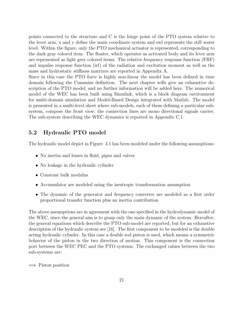
points connected to the structure and C is the hinge point of the PTO system relative tothe lever arm, x and y define the main coordinate system and swl represents the still waterlevel. Within the figure, only the PTO mechanical actuator is represented, corresponding tothe dark gray colored item. The floater, which operates as activated body and its lever armare represented as light grey colored items. The relative frequency response function (FRF)and impulse response function (irf) of the radiation and excitation moment as well as themass and hydrostatic stiffness matrixes are reported in Appendix A.Since in this case the PTO force is highly non-linear the model has been defined in timedomain following the Cummins definition. The next chapter wills give an exhaustive de-scription of the PTO model, and no further information will be added here. The numericalmodel of the WEC has been built using Simulink, which is a block diagram environmentfor multi-domain simulation and Model-Based Design integrated with Matlab. The modelis presented in a multi-level sheet where sub-models, each of them defining a particular sub-system, compose the front view; the connection lines are mono directional signals carrier.The sub-system describing the WEC dynamics is reported in Appendix C.1.

5.2 Hydraulic PTO model

The hydraulic model depict in Figure 4.1 has been modeled under the following assumptions:

• No inertia and losses in fluid, pipes and valves

• No leakage in the hydraulic cylinder

• Constant bulk modulus

• Accumulator are modeled using the isentropic transformation assumption

• The dynamic of the generator and frequency converter are modeled as a first orderproportional transfer function plus an inertia contribution

The above assumptions are in agreement with the one specified in the hydrodynamic model ofthe WEC, since the general aim is to grasp only the main dynamic of the system. Hereafter,the general equations which describe the PTO sub-model are reported, but for an exhaustivedescription of the hydraulic system see [16]. The first component to be modeled is the doubleacting hydraulic cylinder. In this case a double rod piston is used, which means a symmetricbehavior of the piston in the two direction of motion. This component is the connectionport between the WEC PEC and the PTO systems. The exchanged values between the twosub-systems are:

=⇒ Piston position

21

Figure 5.2: Wavestar point absorber WEC

=⇒ Piston velocity

⇐= PTO force

Where the direction of the arrows suggests the carried signals flow direction. If the arrowpoints to the left the information is passed from the WEC submodel to the PTO submodel,and vice-versa. In this case, since the motion of the PEC floater is described by the angular

22

displacement, velocity and acceleration, a conversion function needs to be defined from thegeometry of the system. As it can be seen in Fig. 5.2, three rotational bearing are located inpoint A, B and C, and while point C is moving in time, point A and B are fixed. Therefore it ispossible to calculate the angle between lines AB and AC from the actual angular displacementand its value at the equilibrium, and then solve the so called side-angle-side (SAS) triangle,for further detail see Appendix B. Knowing the length of the actuator lPTO(t) in functionof time is then possible to obtain the bi-univocal conversion between linear and rotationalmotion. The mathematical model of the hydraulic cylinder is basically composed by twoequations. The first describe the evolution in time of the pressure in the piston chamber,calculated from the mass balance for each them, eq 5, while the second one evaluate thePTO force applied on the PEC floater as a force balance on the piston surface, eq 6.

dpAdt

=β(qLPA − qHPA + aA v)

V 0A − aA x

dpBdt

=β(qLPB − qHPB − aB v)

V 0B + aB x

(5)

Where, p is the pressure at the hydraulic piston chamber, β is the Bulk modulus of the usedfluid, qLP is the fluid flow rate from the LP reservoir, qHP is the fluid flow rate to the HPreservoir, a is the piston area, v is the piston velocity, V 0 is the chamber initial volume andx is the piston dispalcement. The subscript A or B indentifies the chamber A or B of thehydraulic piston.

FPTO = −(pA aA − pB aB) (6)

Where, FPTO is the PTO feedback force.

See Appendix C.2 for further details. The outgoing flux from the hydraulic piston needs tobe rectified using check valves. The valves are modeled using a look-up table to relate thepressure difference between the two sides of the valve to the passage area. The piecewisefunction is describes by the following parameters:

• Leakage Area: Describe the leakage of the valve when the pressure across the valve isbelow the cracking pressure

• Maximum Area: Describe the full open valve condition

• Crack Pressure: Describe the minimum pressure at which the system start to open

• Maximum Pressure: Describe the maximum value at which the valve start to close

The flow across the valve is than calculated by eq 7

q(t) = sign(∆p)A(t)CD

√2|∆p(t)|

ρ(7)

23

Where, q(t) is the flow rate across the valve, ∆p is the pressure difference between the twosides of the valve, A(t) is the area of passage of the valve and CD is the check valve coefficientof discharge.In this case the flow is considered to be always turbulent, therefore the low Reynold flowequation has not been used. With the same set of equation it is possible to model the reliefvalve for high pressure and low pressure protection. This constrain are important to keepthe model as realistic as possible but still simple. For this case study these type of systemprotection have been oversized in order to do not overshoot the request pressure set-point.See Appendix C.3 for further details. The two accumulator (HP and LP ones) have beenmodeled as gas accumulator with the assumption of no volume variation of the chamber,incompressible liquid and isentropic transformation, read pV γ = const. The actual volumeof liquid available at the accumulator is calculated from the mass conservation knowing thatthere is only one IN port and one OUT port for the system, with their relative fluid flowrate. Following, the available volume of gas is obtained and used, holding the isentropicrelation, to evaluate the pressure rate of change, eq 8

dpHPdt

=β(qLPA − qHPA + aA v)

V 0A − aA x

dpLPdt

=β(qLPB − qHPB − aB v)

V 0B + aB x

(8)

Where, pHP is the pressure at the HP reservoir and pLP is the pressure at the LP reservoir.An ON/OFF signal of low-low-liquid level (LLL) and high-liquid level (HL) type is sentfrom the HP accumulator to the motor in order to avoid the fill-up or drain-down case. SeeAppendix C.4 for further details. The hydraulic motor used in the model is of the fixeddisplacement kind. For this type of motor the torque at the shaft Tm can be calculated byeq 9

Tm(t) = λ∆p(t) (9)

Where, λ is the volumetric motor displacement. And the motor flow qm can be calculatedby eq 10

qm(t) = λN(t) (10)

Where, N is the rotational speed of the motor. The motor subsystem accepts the ON/OFFsignal coming from the HP accumulator as a bang-bang controller signal. This controlleracts in the following way:

• If 1 the motor torque is calculated by eq 9, the bypass valve is closed

• If 0 the bypass circuit is open with a rate limiter and the motor torque is set graduallyto zero. The motor can keep on spinning and decelerate gradually.

24

As mentioned before the inertia of the motor has been summed to the generator one with-out the inclusion of any shaft stiffness. Since the motor is working only in one quadrantthe rotational speed integrator carries a saturation limit to prevent negative velocity. Thiscan be physically seen as an instantaneous check valve at the motor inlet. In this case thecheck valve has not been physically implemented into the model due to instability causedby the fast dynamic behavior requested. The motor does not include any damping exceptthe emergency brake, because the generator controller was used to tune its applied torqueon the system in order to match the velocity set-point.Due to the fast dynamics of the generator and the frequency converter (FC) with respectto the motor ones, the two systems have been modeled with one single-imput-single-output(SISO) of first-order-process-model (FOPM) type, with constant time of 30ms. This approx-imation is possible only because the ration between the characteristic time of the generatorand motor is smaller than one. The velocity controller is a simple PI controller, tuned usingthe marignal gain method. See Appendix C.5 for further details.In order to analyze the different point of leakages in the transormation chains, the meanpower has been calculated at three different spots: at the pivoting point (Absorbed Power,Pabs), at the HP accumulator (Accumulated Power, Pacc) and at the generator (ElectricalPower, Pel), by (11, 12, 13)

Pabs =1

tend

∫ tend

0

τPTO(t)ω(t)dt (11)

Pacc =1

tend

∫ tend

0

qHP (t)pHP (t) (12)

Pel =1

tend

∫ tend

0

τgen(t)N(t)dt (13)

Where, tend is the simulation time length, τPTO is the torque at the hinging point inducedby the PTO system in the floater and τgen is the torque at the generator shaft. Thesequantities are then normalized by the wave power Pwave, calculated by (14), in order toobtain a non-dimentional system efficiency.

Pwave =ρg2

64πH2m0Tp (14)

Where, Hm0 is the significant wave height and Tp is the peak wave period.

25

6 Simulations

The behavior of the integrated system, composed by the WEC model and the HydraulicPTO model was investigated in irregular long crested waves. The water level to assess thewave body interaction is considered infinity. In particular the scatter diagram relative toHanstholm (DK) was used, which is represented in Table 2. Table 2 report the likelihood of

Table 2: Hanstholm Scatter Diagram

Hm0(m)/TP (s) 0.5 1.5 2.5 3.5 4.5 5.5 6.5 7.50.25 - - - 0.03 0.04 0.03 0.03 -0.75 - - - 0.07 0.16 0.11 0.04 0.021.25 - - - - 0.06 0.11 0.05 0.021.75 - - - - - 0.06 0.056 0.012.25 - - - - - 0.02 0.04 0.012.75 - - - - - - 0.02 0.013.25 - - - - - - - 0.01

occurrence, on annual base, for each pair Hm0/TP . For every sea state, defined by the abovepair, a time series, three hours long, is generated using the white noise method [17]. Thesample frequency is set to 4 Hz. In order to evaluate the annual power production the scatterdiagram is then multiplied by the power production matrix, obtained from the simulations.The floater motion is not controlled and the only controllable parameter was the initial andmean pressure on the HP accumulator. The full power matrix has been assessed for fivedifferent pressure levels at the HP accumulator:

• (pressure stage 1) P1 - 10 bar





This can be seen as a slow controller for the system, which can be tuned on hour base. ThePTO characteristics are recapped in Table 3

The system of equation were solved using a variable order solver based on the numericaldifferentiation formulas, ode15s. The Runge-Kutta method with order 4 showed instabilityand a solver for stiff problem was chosen.

26

Table 3: Hydraulic Model Parameters

Hydraulic PistonΥ dpist drod Vdead β p0 psat

[m] [m] [m] [m3] [Pa] [Pa] [Pa]3 0.1 0.05 0.001 1.66e9 1e5 1e4

Check Valve and Bridge RectifierCD ρ Aleak Amax pcrack pmax[−] [kg/m3] [m2] [m2] [Pa] [Pa]0.7 800 1e-12 0.8e-3 1e2 15e3

AccumulatorsV V0

HP V0LP p0

HP p0LP pmax

[m3] [m3] [m3] [Pa] [Pa] [Pa]1 0.3 0.7 variable 1e5 400e5

Motor and Generatorα Tk Nmax JMG qmin

[m3] [N/bar] [rpm] [kgm2] [m3/s]3.5e-6 0.35 4250 1.5e-3 1e-9

27

7 Results and Discussions

The main outcome of the simulations is reported in Fig. 7.1 and Fig. 7.2, where the annualpower production and mean efficiency, in terms of electrical power, is shown as a functionof the HP pressure. The subplots are related to the five pressure classes used, as reported

Figure 7.1: Annual power matrix of the simulated scatter diagram for each pressure condi-tion. The top-left figure represents the scatter diagram of the selected loaction. The colormap is defined by the probability of occurrence. The other five plots report the annualpower matrix, and their color map is the power produced times the related probability inkW. White areas represent condition with negligible power poroduction

28

Figure 7.2: Mean efficiencies for the simulated scatter diagram for each pressure condition.The top-left figure reports the incoming wave power in kW. The other five plots report theefficiency of the device in function of the wave state in %. White areas represent conditionwith negligible power poroduction

in the relative subtitle.Figure 7.1 reports the annual power production matrix for all the tested conditions. InFig. 7.1, position 1x1 is occupied by the scatter diagram of the considered location, whilethe other five plots report the annual power production matrix. At a first glance it is possibleto notice a relative wide white area in the scatter diagram, caused by the absence of energyat those particular H/T pairs, and an even bigger white area for the power matrix. This is

29

mainly linked to the level of pressure set-up in the simulation, which prevent the system tomove. Literally the hydraulic PTO system induce a modification of the dynamical modelof the floater and contrain the system to move when the incoming energy is not sufficientto overcome the energy level at the HP reservoir. The scatter diagram shows a peak atTp = 5.5s and Hs = 1 m, which coincides with the natural period of the WEC simulated.De facto, during the design process the device was geometrically and structurally definedto match the predominant wave condition al thespecific location. As expected from theconsiderations above, the highest power production typically happens at periods close to 5.5s, with a secondary peak located at 6.5 s. The nature of this secondary peak needs to befurther investigated.If we consider only one pressure level, the maximum annual production is achieved at thepressure stage 2 or 3. At the lower pressure stage, the volume of the HP accumulator,the set-point pressure of the relief valve and the hydraulic motor characteristics bound thepower production. In fact due to the reduced PTO feedback force, the motion of the floateris higher, which induces a high flow rate pumped from the hydraulic piston to the HP accu-mulator, which is higher than the motor flow rate. In general at the lower pressure stage thevolumetric design of the accumulator and motor seem to be not appropriate. It is importantto bear in mind that there was no optimization of the proposed design, which should be atrade-off in order to achieve the best overall efficiency.At pressure stage 4 and 5 the overall power production is slightly reduce, because the highestpower density is balanced by the smaller working area. This behavior is directly linked tothe increased PTO feedback force, which constrains the system motion.

Fig. 7.2 reports the efficiency of the tested case, calculated as the ratio between the producedelectrical power and the incoming wave power. This last is a function of the pair H/T andthe device length. In Figure 7.2 position 1x1 is occupied by the incoming wave power matrix.The efficiency of the system is somewhere around 0.2 and 0.35 in all the tested cases, inlinewith the efficiency measured on the real device, deployed in Hanstholm. The highest valueis observable at pressure stage 2 and 3, for a peak wave period around 5 s. Also in this case,stage 1, 4 and 5 seems to be a non-optimal global solution.

It is worth to collect the highest value for each sea state into a global picture, Fig. 7.3.In general this is true if we assume the presence of a controller into the HP accumulator.The task of this controller is to slowly change the pressure into the HP reservoir in accor-dance with the incoming sea state. The controller period will be somewhere around 1-3h.The controlled variable should be the motor speed or its swept volume.Fig. 7.3 shows an hypotethic optimal annual power matrix. Comparing the annual powerproduction for each of the tested pressure stage, with the overall matrix an improvement of10% can be achieved.

All the results reported above are related to the electrical power production. Therefore,

30

Figure 7.3: Optimal annual power matrix for the simulated scatter diagram. White areasrepresent condition with negligible power poroduction

it is worth to understand the presence of any bottleneck/point of losses in the transforma-tion chains, which goes from the incoming wave power to the electrical generated power. Forthis purpose, the power have been assessed at three different locations:

• absorbed power at the floater

• accumulated power into the HP accumulator

• electrical power at the generator

Table 7 reports the efficiency ordered as follow: in the rows, the different wave states, withthe relative pair H/T, and in the columns, the pressure levels tested. For each pressure level,the three different efficiencies, introduced above, are listed. A color map between low (0%,green) and high (35%, red) efficiency value is used. The results summarized in Table 7 canbe recapped in three points:

31

Table 4: Efficiency loss through the transformation chain. The absorbed power at the floater(Pabs), the accumulated power at the HP reservoir (Pacc) and the electrical power (Pel) arereported for each pressure condition and sea state.

• 65%, at the best, of the incoming energy is lost on the wave-body interface. This resultis inline with the result presented by [18]

• The energy transformation from kinetic (floater motion) to pressure (potential accu-mulated at the HP accumulator) does not induce any losses.

• In the worst case 3% of the accumulated energy is lost in the motor/generator block

A closer look at the data reveals that in some case the accumulated power overtake theabsorbed power, by 0.1%. This result can be mainly addressed to the simulation inaccuracyrelated to the highly non-linear system of equations. In particular the fluid compressibilitycauses high frequency oscillation that are cut by the simulation step width. The results aboveare strongly correlated to the PTO characteristics summarized in Table 3. For example, theratio between leakage and maximum area of the check valve is 1e-9, which entails no back-ward flux and no energy loss in the valve stage. The pipe connections and valves losses areconsidered negligible, but they can be simulated using a lumped model as reported in [5]. It isimportant to bear in mind that, the PTO design optimization was not the scope of this work.

As introduce above, the dynamical model of the floater is highly affected by the presence ofthe hydraulic PTO system. Fig. 7.4 shows the power spectral density trends for ws14 andpressure stage 2. The lines represent the normalized power spectral density (PSD) of the

32

angular acceleration, velocity and position, the surface elevation, and the radiation, restor-ing and PTO moments. The normalization was used only for graphical reasons. A zoomedview is also given in the plot area, in order to emphasize the secondary dynamic. The effect

Figure 7.4: Normalized power spectral density (PSD) of the time series relative to ws14 andpressure stage 2. The zoomed view represent the low frequency range.

depicted in Fig. 7.4 highlights the influence of the PTO dynamic on the system, which ismainly caused by the stiffness of the PTO. This last is affected by the fluid compressibil-ity, check valves dynamic, pressure level at the accumulator, gas compressibility, etc., andchanges in time. The main effect is visible in the acceleration signal and it can create fatigueproblem on the structure.

33

Since the utilization of an hydraulic PTO with accumulator is mainly related to the reductionof the generated power pulsation, some important consideration can be extracted from theevolution in time of the HP accumulator pressure and the generated power. Fig. 7.5 showsthe time evolution of the HP accumulator pressure for five different sea state and Fig. 7.6shows the generated power for the same conditions. All the conditions reported are at thepressure stage 2 (50 bar). From a general point of view it is possible to find the best match,

Figure 7.5: Time evolution of the istantanous pressure at the HP accumulator for five seastates. Color lines specification is given in the legend

between PTO configuration and sea state, somewhere around ws12 and ws14, see Table 7for the sea state specification. At lower sea states, such as ws5 and ws8, the hydraulic motorseems to be over-sized, causing an unwanted power pulsation. In fact the energy take more

34

Figure 7.6: Time evolution of the instantaneous electrical power for five sea states. Colorlines specification is given in the legend

time to build-up than the time required to be consumed. On the contrary, for higher seastate, such as ws21, the motor seems to be under-sized, which cause the pressure to reach therelief valve set point. This event can be clearly seen in Fig. 7.5 at time 900s. The relief valveis set in such a way that the initial pressure condition is restored when the valve open, inorder to avoid the so-called chattering, which in turn cause the simulation to slow down. Thefixed displacement motor allows the best performance only in the intermediate sea states.In this range the generated power pulsation is highly reduced, compared with the absorbedpower. The behavior of ws12 still presents pulsations, but the time band for the motoris on condition, is higher than the motor-off one. An improvement of the electrical powergeneration can be achieved in this case by simply changing the motor/generator control ar-

35

chitecture. In general both the figures shows the need of increase the system flexibility, inorder to enlarge the match between incoming energy and absorbable energy. Either changingthe PTO architecture or adding a variable displacement motor can do this. Another way toincrease the system efficiency is to allow the motor speed to change, because the generatorwith FC can meanage speed variations. On the other hand changing the fixed displacementmotor size it is not a solution, because it will only change the working range position, andnot its area.

36

8 Conclusion

The present report gave a general overview of the hydraulic PTO systems. Nowadays, theinterest on this type of systems for applications in the wave energy field is mainly relatedto the lack of a real/reliable alternative to convert the absorbed power into electricity. Infact, the principle of avoiding prototype on prototypes, defines the need of a well vaidatedPTO technology. Hydraulic PTO systems are extensivelly studied, because they are robustand their features match the wave energy ones, i.e. low period and high loads. Differenthydraulic PTO architectures have already been studied in the last year. In this specificwork, type 1 has been implemented. The system is composed by a double action hydraulicpiston, a rectifying bridge of check-valves, a HP and LP accumulators, a hydraulic fixeddisplacement motor and a generator. The fluid compressibility is implemented using thefluid bulk modulus. The model implemented shows different limitations, i.e. poor flexibilitywith respect to the incoming sea state, even if this was not the scope of the work, whichcause the system to be far away from its optimal configuration. In any case the performanceof the model are in line with the Wavestar prototype installed in the Nord Sea. This typeof PTO system induces a deep modification of the hydrodynamic model, causing motionconstrains, fast and secondary dynamics, and high loads on the floater arm.

37

References

[1] R. Henderson, “Design, simulation and testing of a novel hydraulic power take-off systemfor the pelamis wave energy converter,” Renewable Energy, vol. 31, pp. 271–283, 2006.

[2] J. Lasa, J. C. Antolin, C. Angulo, P. Estensoro, M. Santos, and P. Ricci, “Desing,construction and testing of a hydraulic power take-off for wave energy converters,”Energies, vol. 5, pp. 2030–2052, 2012.

[3] Y. Kamizuru, L. Verdegem, P. Erhart, C. Langenstein, L. Andren, M. LenBen, andH. Murrenhoff, “Efficient power take-offs for ocean energy conversion,” in ICOE,(Dublin), 2012.

[4] A. F. d. O. Falcao, “Modelling and controll of oscillating-body wave energy convert-ers with hydraulic power take-off and gas accumulator,” Ocean Engineerign, vol. 34,pp. 2021–2032, 2007.

[5] K. Schlemmer, F. Fuchsumer, N. Boemer, R. Costello, and C. Villegas, “Design andcontroll of a hydraulic power take-off for an axi-symmetric heaving point absorber,” inEWTEC, (Southampton), 2011.

[6] J. Hals, R. Taghipour, and T. Moan, “Dynamics of a force-compensated two-body waveenergy converter in heave with hydraulic power take-off subject to phase control,” inEWTEC, (Porto), 2007.

[7] H. Eidsmoen, “Simulation od a slack-moored heaving-buoy wave-energy converter withphase control,” 1996.

[8] H. Eidsmoen, “Simulation od a tight-moored amplitude-limited heaving-buoy wave-energy converter with phase control,” 1996.

[9] C. Josset, A. Babarit, and A. H. Clement, “A wave-to-wire model of the searev waveenergy converter,” Journal of Enginnering for the Maritime Environment, vol. 81, 2007.

[10] R. Costello, J. V. Tingwood, and J. Weber, “Comparison of two alternative hydraulicpto concepts for wave energy conversion,” in EWTEC, (Southampton), 2011.

[11] Y. Kamizuru, M. Lermann, and H. Murrenhoff, “Simulation of an ocena wave en-ergy converter using hydraulic transmission,” in International Fluid Power Conference,(Aachen), 2010.

[12] A. F. d. O. Falcao, P. A. P. Justino, J. C. C. Henriques, and J. M. C. S. Andre, “Reactiveversus latching phase control of a two-body heaveing wave energy converter,” 2008.

38

[13] G. Bacelli and J. V. Ringwood, “A control system for a self-reacting point absorberwave energy converter subject to constrains,” in IFAC, (Milan), 2011.

[14] P. Ricci, J. Lopez, M. Santos, J. L. Villate, P. Ruiz-Minguela, F. Salcedo, and A. F.d. O. Falcao, “Control strategy for a simple point absorber connected to a hydraulicpower take-off,” in EWTEC, (Uppsala), 2009.

[15] W. E. Cummins, “The impulse response function and ship motion,” in Symposium onShip Theory, (Hamburg), 1962.

[16] H. E. Merrit, Hydraulic control system. New York: John Wiley and Sons, 1967.

[17] P. Frigaard, M. Hogedal, and C. M, Wave generation theory. Aalborg: Aalborg Univer-sity, 1993.

[18] M. M. Kramer, L. Marquis, and P. Frigaard, “Performance evaluation of the wavestarprototype,” in EWTEC, (Southempton), 2011.

39

Appendices

A Wavestar: Hydrodynamic and hydrostatic parame-

ters

Moment of Inertia (J): [kgm2]2.45*106

Hydrostatic Restoring Moment (kh): [Nm/rad]14.0*106

Figure A.1: Radiation moment frequency response function: Damping (full draw line) andAdded Mass (dotted line) in function of the frequency of the motion

40

Figure A.2: Excitation moment frequency response function: Magnitude (full draw line) andPhase (dotted line) in function of the frequency of the incoming waves

41

B PTO length

α is the angle in A, which can be obtained from the angular displacement θγ is the angle in Cβ is the angle in B

BC =

√AB

2+ AC

2 − 2AB · AC · cos(α)

K = sin(α) · AB · ACBC

K is the moment arm

42

C Simulink Model

C.1 Simulink Submodels: Floater

43

C.2 Simulink Submodels: Hydraulic Piston

44

C.3 Simulink Submodels: Check Valves Bridge Rectifier

45

C.4 Simulink Submodels: HP and LP accumulators

46

C.5 Simulink Submodels: Motor and Generator

49

Implementation of a Hydraulic Power Take-Off for … D4.7 ISSN 1901-726X DCE Technical Report No....

Documents

Transcript of Implementation of a Hydraulic Power Take-Off for … D4.7 ISSN 1901-726X DCE Technical Report No....