Implementation of a 3D Graphics Rendering Pipeline Using...
84
CALIFORNIA STATE UNIVERSITY, NORTHRIDGE IMPLEMENTATION OF A 3D GRAPHICS RENDERING PIPELINE USING A FIELD PROGRAMMABLE GATE ARRAY A graduate project submitted in partial fulfillment of the requirements for the degree of Master of Science in Electrical Engineering By Vahe Jabagchourian December 2011
Transcript of Implementation of a 3D Graphics Rendering Pipeline Using...

CALIFORNIA STATE UNIVERSITY, NORTHRIDGE
IMPLEMENTATION OF A 3D GRAPHICS RENDERING PIPELINE
USING A FIELD PROGRAMMABLE GATE ARRAY
A graduate project submitted in partial fulfillment of the requirements
for the degree of Master of Science
in Electrical Engineering
By
Vahe Jabagchourian
December 2011

ii
Signature Page
The graduate project of Vahe Jabagchourian is approved:
Xiaojun (Ashley) Geng, Ph.D. Date
Shahnam Mirzaei, Ph.D. Date
Ramin Roosta, Ph.D. Date
Ronald W. Mehler, Ph.D., Chair Date
California State University, Northridge

iii
Acknowledgements
I would like to thank Dr. Mehler for agreeing to serve as the committee chair and for providing valuable
feedback throughout the duration of the project. I would also like to thank Dr. Mirzaei for his assistance in
the area of Field Programmable Gate Array development and for providing helpful suggestions.
Additionally, I would like to thank Dr. Geng and Dr. Roosta for agreeing to serve on the committee.
Finally, I would like to thank my parents, Harry and Silvia, and my brother, Vatche, for their support and
encouragement.
iv
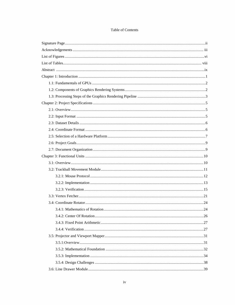
Table of Contents
Signature Page .................................................................................................................................................ii Acknowledgements ....................................................................................................................................... iii List of Figures ................................................................................................................................................ vi List of Tables............................................................................................................................................... viii Abstract ......................................................................................................................................................... ix Chapter 1: Introduction ................................................................................................................................... 1
1.1: Fundamentals of GPUs ..................................................................................................................... 2 1.2: Components of Graphics Rendering Systems ................................................................................... 2 1.3: Processing Steps of the Graphics Rendering Pipeline ...................................................................... 3
Chapter 2: Project Specifications .................................................................................................................... 5 2.1: Overview ........................................................................................................................................... 5 2.2: Input Format ..................................................................................................................................... 5 2.3: Dataset Details .................................................................................................................................. 6 2.4: Coordinate Format ............................................................................................................................ 6 2.5: Selection of a Hardware Platform ..................................................................................................... 7 2.6: Project Goals ..................................................................................................................................... 9 2.7: Document Organization .................................................................................................................... 9
Chapter 3: Functional Units .......................................................................................................................... 10 3.1: Overview ......................................................................................................................................... 10 3.2: Trackball Movement Module .......................................................................................................... 11
Mouse Protocol ..................................................................................................................... 12 3.2.1:
Implementation ..................................................................................................................... 13 3.2.2:
Verification ........................................................................................................................... 15 3.2.3:
3.3: Vertex Fetcher ................................................................................................................................. 21 3.4: Coordinate Rotator .......................................................................................................................... 24
Mathematics of Rotation ....................................................................................................... 24 3.4.1:
Center Of Rotation ................................................................................................................ 26 3.4.2:
Fixed Point Arithmetic .......................................................................................................... 27 3.4.3:
Verification ........................................................................................................................... 27 3.4.4:
3.5: Projector and Viewport Mapper ...................................................................................................... 31 3.5.1:Overview ................................................................................................................................ 31 3.5.2: Mathematical Foundation ..................................................................................................... 32 3.5.3: Implementation ..................................................................................................................... 34 3.5.4: Design Challenges ................................................................................................................ 38
3.6: Line Drawer Module ....................................................................................................................... 39
v
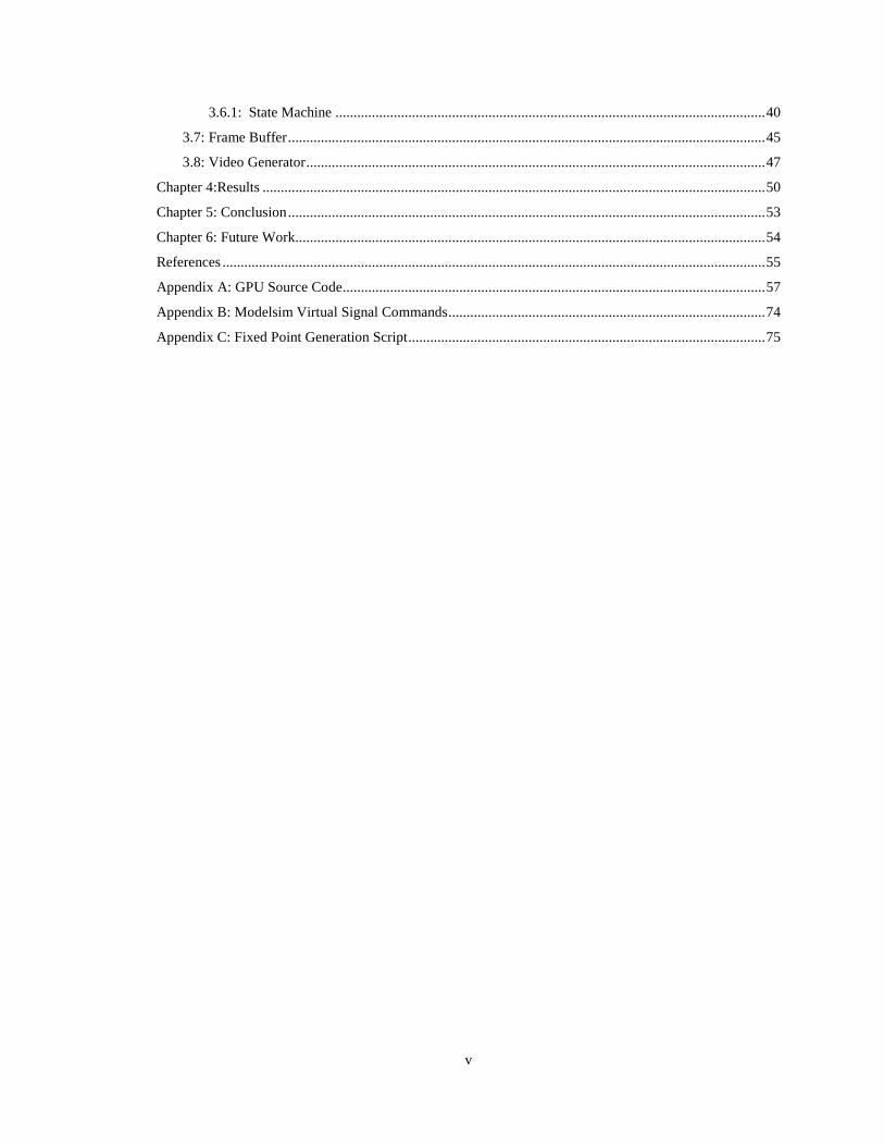
3.6.1: State Machine ...................................................................................................................... 40 3.7: Frame Buffer ................................................................................................................................... 45 3.8: Video Generator .............................................................................................................................. 47
Chapter 4:Results .......................................................................................................................................... 50 Chapter 5: Conclusion ................................................................................................................................... 53 Chapter 6: Future Work ................................................................................................................................. 54 References ..................................................................................................................................................... 55 Appendix A: GPU Source Code .................................................................................................................... 57 Appendix B: Modelsim Virtual Signal Commands ....................................................................................... 74 Appendix C: Fixed Point Generation Script .................................................................................................. 75

vi
List of Figures
Figure 1: Top level block diagram of the Graphics Rending System ............................................................. 1
Figure 2: Five Components of a Graphics Renderer [1] .................................................................................. 3
Figure 3: GPU Functional Unit Breakdown [2] ............................................................................................. 4
Figure 4: OFF Dataset Syntax and Teapot Dataset Snippet ........................................................................... 6
Figure 5: 14-Bit X and Y coordinates (Fraction 1.99 in Sign Magnitude Fixed Point) ................................... 7
Figure 6: 14-Bit Depth (Z) Coordinate (Fraction 3.99 in Sign Magnitude Fixed Point) ................................ 7
Figure 7: System Level Block Diagram of 3D Graphics Rendering Pipeline ............................................... 10
Figure 8: Top Level Schematic of the Original PS/2 Tx/Rx Unit Shown as Separate Blocks ..................... 11
Figure 9: Device to Host Communication (Data Bit Read on Rising Edge of Clock) [13] .......................... 12
Figure 10: Host to Device Communication (Data Bit Read on Falling Edge of Clock) [13] ....................... 12
Figure 11: PS/2 Communication Protocol [14] ........................................................................................... 12
Figure 12: Depiction of 4 byte packets transmitted from mouse to host FPGA [14] ................................... 14
Figure 13: Simplified Mouse Initialization/Streaming Controller State Machine ........................................ 15
Figure 14: LED arrangement on the XUPV5-LX110T for debugging direction and position ..................... 16
Figure 15: User Constraints File for PS/2 Module ....................................................................................... 16
Figure 16: Mouse Initialization Behavioral Simulation ............................................................................... 17
Figure 17: Mouse Initialization (Part 2) Behavioral Simulation .................................................................. 18
Figure 18: Streaming Packets from PS2 Mouse (Y Movement) .................................................................. 19
Figure 19: Streaming Packets from PS2 Mouse (X Movement) .................................................................. 20
Figure 20: Vertex Fetcher Controller Block Diagram (Inputs on Left, Outputs on Right) .......................... 21
Figure 21: Original Static Pyramid – Shape Generator State Machine without clear states ......................... 22
Figure 22: Original Static Four Line Shape Generator State Machine with Clear States ............................. 22
Figure 23: Vertex Fetcher State Machine ..................................................................................................... 23
Figure 24: Coordinate Rotator Block Diagram ............................................................................................ 24
Figure 25: Summary of rotation options for trackball input device.............................................................. 26
Figure 26: Behavioral Simulation (Analog Step) of Sin/Cos ROM ............................................................. 28
Figure 27: Behavioral Simulation (Analog Step) of Rotator Multipliers ..................................................... 29
Figure 28: Verification (Analog Step) of Rotation Module (Simulated versus Actual) ............................... 30
Figure 29: One point perspective convergence [19] ..................................................................................... 31
Figure 30: Viewport Transformation and Scaling [20] ................................................................................ 31
Figure 31: 3D Pyramid alongside its projected representation ..................................................................... 34
Figure 32: Initial Integration of Coordinate Generator, Viewport Projector and Rasterizer ........................ 35
Figure 33: Projector / Viewport Mapper Block ............................................................................................ 35
Figure 34: Internal Blocks of the Coordinate Projector and Viewport Mapper ............................................. 35

vii
Figure 35: Behavioral Simulation of Fetcher/Projector with Several Line Vertices Generated ................... 36
Figure 36: Behavioral Simulation of Fetcher/Projector with a single line endpoint shown ......................... 37
Figure 37: High Speed Division by Reciprocal Multiplication [23]............................................................. 38
Figure 38: Perspective Divider (using Reciprocal Lookup Multiplication Method) ..................................... 38
Figure 39: Depiction of a Rasterized Line with a positive slope [24] .......................................................... 39
Figure 40: Bresenham Rasterizer pseudo code [25] ..................................................................................... 40
Figure 41: State Machine for Line Generator Block .................................................................................... 41
Figure 42: Top Level Block Diagram of Line Generator ............................................................................. 42
Figure 43: Implementation tasks for the Static Line Generator .................................................................... 42
Figure 44: Implementation tasks for the Dynamic Line Generator .............................................................. 43
Figure 45: Results from Cursor Position Based Line Generator .................................................................. 43
Figure 46: Behavioral Simulation of Single Line Generator ........................................................................ 44
Figure 47: SRAM Interface versus DPRAM Module .................................................................................. 45
Figure 48: Final Frame Buffer Architecture (14 of 64 buffers presented).................................................... 46
Figure 49: I2C Protocol [26] ........................................................................................................................ 47
Figure 50: Video Timing Diagram ............................................................................................................... 48
Figure 51: Video Generator ........................................................................................................................... 48
Figure 52: Pixel Multiplexer (Input to Chrontel 7301C) .............................................................................. 49
Figure 53: Orthographic (parallel) projected teapot ...................................................................................... 50
Figure 54: Perspective (convergent) projected teapot .................................................................................. 50

viii
List of Tables
Table 1: Hardware Requirements Compliance Matrix ................................................................................... 8
Table 2: GPU System Level Breakdown ...................................................................................................... 10
Table 3: Trackball Controller States and Transmission Values [14] ............................................................ 13
Table 4: Depiction of when to add 2.5 to Z (Refer to Figure 24 for red and green signal locations) ........... 26
Table 5: Fixed Point Arithmetic Conditions [18] ......................................................................................... 27
Table 6: Summary of parameters for viewport transformation .................................................................... 33
Table 7: Line Generator State Description ................................................................................................... 41
Table 8: Video Parameters ........................................................................................................................... 47
Table 9: Summary of Object Parameters ...................................................................................................... 50
Table 10: Application of rotation transformation with various angles .......................................................... 51
Table 11: Rotation across both x and y ........................................................................................................ 52
ix
ABSTRACT
IMPLEMENTATION OF A 3D GRAPHICS RENDERING PIPELINE
USING A FIELD PROGRAMMABLE GATE ARRAY
By
Vahe Jabagchourian
Master of Science in Electrical Engineering
The objective of this project was to produce a working design of a 3D graphics rendering pipeline
using an FPGA (Field Programmable Gate Array) and to develop proficiency in the development of a
digital design using Verilog Hardware Description Language. The FPGA is loaded with the bitstream of
the GPU (Graphics Processing Unit) which produces an object on an LCD monitor. The final deliverable is
Verilog source code describing the GPU which has been implemented on a Virtex-5 LX110T FPGA
development board. The input to the FPGA is a bidirectional serial PS/2 signal which passes data back and
forth between FPGA and trackball. The output from the FPGA is a digital video signal which displays a
projected object on a monitor where the orientation can be changed when a new dataset configuration is
loaded. Finally, the design provides a method to load in new datasets and initialize on-chip Block RAM
content with the datasets. The primary functional units of the 3D rendering pipeline include the vertex
fetcher unit, rotation unit, mouse movement unit, projection unit, perspective division unit, viewport
mapping unit, line drawing unit and video generation unit.

1
Chapter 1: Introduction
Computer graphics describes the process by which points are converted into pixels. Specialized
hardware called Graphical Processing Units (GPU) convert 3D geometric objects into a 2D representation
that is displayed on a monitor. GPUs are manufactured on Application Specific Integrated Circuits
(ASICs) commercially and on Field-Programmable Gate Arrays (FPGAs) for rapid-prototyping and
hardware emulation. FPGAs are hardware chips that contain specialized blocks of logic, and specialized
hardware components for performing virtually any type of logic function. The advantage of FPGAs over
ASICs is that FPGAs can be re-programmed many times which makes them customizable and well suited
for academic and research projects. Since FPGAs are reprogrammable and have a simpler design cycle
than ASICs, they are used in rapid prototyping applications. Figure 1 shows the FPGA development board
(XUPV5-LX110T) that has been selected for this project. It contains the Xilinx Virtex-5 FPGA, which is
used in high speed embedded applications. It can be configured to run a standalone digital design that
connects to on board peripherals or run a hardware/software co-design with C code alongside an embedded
(on-chip) processor.
Figure 1: Top level block diagram of the Graphics Rending System
Information about the board provided from www.xilinx.com includes the following common applications
for the XUPV5-LX110T1 FPGA
1. Digital Design
2. Embedded Systems
3. Digital Signal Processing and Communications
4. Computer Architecture
5. Operating Systems
6. Networking
7. Video and Image Processing
8. High Speed Serial I/O Transceivers
1Details about the V5LX110T can be found at http://www.xilinx.com/products/boards-and-kits/XUPV5-LX110T.htm
DVI Link PS/2 Link
Digital Monitor Xilinx Virtex-5 FPGA Board Trackball Mouse

2
1.1: Fundamentals of GPUs
A GPU is a commonly used acronym for Graphics (or Graphical) Processing Unit. GPUs are
specialized primarily for rendering and visual applications such as medical visualization or high
performance computing. A special type of GPU called GPGPU (General Purpose GPU) is used to refer to
Graphical Processing Units that can perform a non-specific function compared to a classical GPU. The
focus of this project is to develop a prototype of a classical single core graphical processor for display
applications.
Computer graphics is the process of displaying information. Displaying information means
representing 3D information on a 2D space such as a computer monitor. The primary input to a computer
graphics system is a set of coordinates. The main use of a computer graphics system can be seen in
applications such as display systems, design of interactive handheld devices, smart phones and human
computer interaction systems. In each of these applications the user of the system needs to see a visual
representation of the data to facilitate the interaction process. In medical imaging systems, for example, the
medical technician is working to interpret a 3D graphical representation of a dataset. The visualization
system is producing high-quality images at a high speed using modern graphics rendering hardware. In
other applications such as general purpose computing, or simulation, the end user is using the visual display
as a guide to be able to control and see what is going on with his/her input commands. When pilots train
for flight, they often rely on virtual-reality systems to help simulate conditions that are present in the real
flight. These virtual-reality systems, computer platforms and medical systems represent a sample of the
applications seen in computer graphics. The goal of any graphics system is to convert points to pixels
which provide a visual way of interpreting large amounts of numerical data.
Graphical Processing Units that output graphical data operate on large amounts of vertex points which
are sent off to a monitor or host processor for display or processing. GPUs differ from CPUs in that they
are inherently designed to operate on large amounts of data in parallel. GPUs can achieve greater speed
than CPUs because they are designed with greater amount of functional units and dedicated memory.
Because of the sheer number of parallel processing units on GPUs as compared to CPUs, there is a great
performance disparity when running instructions on GPUs that are programmable rather than conventional
CPUs.
1.2: Components of Graphics Rendering Systems
Computer graphics renderers display information. The hardware that makes a graphics system work is
similar to the five components of a computer (Memory, Input, Output, ALU and the CPU). The
components of a graphics system are depicted in Figure 2. The input device can be a mouse, trackball,

3
sensor, or even a camera or any device that acquires information. The memory block is used to store the
vertices of the object. The GPU is the focus of the project and it consists of functional units which alter the
points passed through the pipeline. The frame buffer receives the data from the GPU and sends it to an
output device. An output device can be a monitor, for example.
Figure 2: Five Components of a Graphics Renderer [1]
1.3: Processing Steps of the Graphics Rendering Pipeline
A classical rendering pipeline begins with the acquisition of data points (vertices) and ends with the
production of pixels on a screen. The internal components of the pipeline are what constitute the GPU.
The first stage in the classical rendering pipeline is the transformer. The transformer receives a set of
vertex coordinates and performs mathematical transformations such as translation, rotation or scaling.
There are other transformations including shearing that alter the original shape of the object. A
transformation matrix which contains the information for transforming input coordinates to output
coordinates is the basis for many of the hardware blocks in the graphics system.
After the object is modeled (translated, rotated, scaled) it is then viewed which means that the object
changes representation from world coordinate system to the eye or camera coordinate system. This usually
involves projecting the object onto a 2D space where the object undergoes further manipulations.
Transformation, which consists of modeling and viewing, embodies the first of the four transformations in
the classical rendering pipeline. The next step is called the clipping stage. A clipper trims portions of the
object which are not in the viewing space (the 2D plane of projection). There are many algorithms to
accomplish the clipping process and they usually consist of a pipeline which performs a left trim, a right
trim, and finally a top and bottom trim. At each trim stage the coordinates of intersection are calculated
Input GPU Frame Buffer Output
Memory

4
and then used to reshape the object to have edges that are the same as the bounding edges. After an object
is clipped, it is projected onto the device space that serves as the viewing space for the object.
There are different types of projections and they include Orthographic Projections and Perspective
Projections. The Orthographic Projection consists of parallel projection where the center of projection is at
infinity. Perspective projections have their center of projection at a finite distance from the viewing plane.
It is easier to perform orthographic projection because there is no need to perform perspective correction.
The projection matrix for an orthographic matrix converts the depth (z coordinate) value to zero and
preserves the x and y coordinates of the shape. After projected onto the projection space the rasterizer
performs the main drawing function of the renderer. Figure 3 breaks down the functional units of the
graphics rendering pipeline.
Four processing steps of a graphics renderer include:
1. Application – Reads memory of object vertices and sends to transformation unit
2. Geometry – Performs geometric transformations on object and maps to screen space
3. Rasterization – Calculates line shape pixels, fills object with a solid or shaded color
4. Display – Reads from frame buffer generates video synchronization and multiplexed RGB data
Application Geometry Rasterization Display Read in 3D Data Geometric Transform Clipping/Scissoring Read Frame Buffer Write to Registers Perspective Division Line Generation Generate HV Sync Stream to Geometry Screen Mapping Store in Frame Buffer Multiplex RGB Data
Figure 3: GPU Functional Unit Breakdown [2]
Application Geometry Rasterization Display

5
Chapter 2: Project Specifications
2.1: Overview
The objective of this project was to produce a GPU design in Verilog and implement the design on an
FPGA. The GPU accepts a 3D dataset at compile time (during behavioral elaboration) and outputs a
projected image on the monitor. The first requirement is to select an appropriate FPGA development board
with sufficient resources. The second requirement is to provide capability to easily import in different
dataset (binary valued lookup tables using a real to fixed point converter function). In addition, the design
supports the storage of a relatively complex dataset. It also renders the object on a digital monitor. Finally,
the object is able to be rotated using compile time rotation equations which show the rotated object on the
monitor. Use of Verilog Hardware Description Language was the main component of the project. In
addition, use of binary conversion scripts in Verilog and other scripting languages have aided in producing
a quick memory initialization file for testing the design on the FPGA. Tools used in the project include
Matlab, Microsoft Excel, Xilinx synthesis, design entry and simulation tools to verify and implement the
design on the Virtex-5 board.
Summary of Requirements
1. Utilize an FPGA with sufficient resources to run the GPU design
2. Employ chip Block RAMs as a Frame Buffer for Wireframe rendering
3. Perform computations using pre-computed fixed-point lookup tables
4. Execute rotation transformation with ability to modify functionality for transformation
5. Provide for addition of extra modules such as double-buffering to reduce flickering
6. Allow entry of arbitrary dataset during design and implementation
2.2: Input Format
Originally, a simple four-sided pyramid of triangles was hard coded into a state machine and it consisted
of four states. The state machine was a four vertex pyramid. The state machine proved to be a quick way
of generating the object. Though this method is quick to write, it was later improved and even scaled by
segregating the data from the logic. Eventually, a reasonably sized dataset was located and a vertex
fetching state machine was created and two blocks of memory (object vertices and triangle vertex
coordinates) was created to provide an easy way to change the object. Verilog and especially Xilinx XST
(synthesis tool) allows the initialization of Dual Port Block Rams using memory (mem) files for FPGA
applications. The dataset used for testing the GPU consists of two files (“vertices.mem” and
“triangles.mem”) created from an OFF dataset. The original memory file was an object file format based
dataset which is used in a UNIX graphical rendering program called GeomView.
6
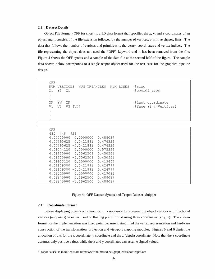
2.3: Dataset Details
Object File Format (OFF for short) is a 3D data format that specifies the x, y, and z coordinates of an
object and it consists of the file extension followed by the number of vertices, primitive shapes, lines. The
data that follows the number of vertices and primitives is the vertex coordinates and vertex indices. The
file representing the object does not need the “OFF” keyword and it has been removed from the file.
Figure 4 shows the OFF syntax and a sample of the data file at the second half of the figure. The sample
data shown below corresponds to a single teapot object used for the test case for the graphics pipeline
design.
OFF NUM_VERTICES NUM_TRIANGLES NUM_LINES #size X1 Y1 Z1 #coordinates . . XN YN ZN #last coordinate V1 V2 V3 [V4] #face (3,4 Vertices) . . .
OFF 480 448 926 0.00000000 0.0000000 0.488037 0.00390625 0.0421881 0.476326 0.00390625 -0.0421881 0.476326 0.01074220 0.0000000 0.575333 0.01250000 0.0562508 0.450561 0.01250000 -0.0562508 0.450561 0.01953120 0.0000000 0.413654 0.02109380 0.0421881 0.424797 0.02109380 -0.0421881 0.424797 0.02500000 0.0000000 0.413086 0.03875000 0.1962500 0.488037 0.03875000 -0.1962500 0.488037
Figure 4: OFF Dataset Syntax and Teapot Dataset2 Snippet
2.4: Coordinate Format
Before displaying objects on a monitor, it is necessary to represent the object vertices with fractional
vertices (endpoints) in either fixed or floating point format using three coordinates (x, y, z). The chosen
format for the implementation was fixed point because it simplified the vertex representation and hardware
construction of the transformation, projection and viewport mapping modules. Figures 5 and 6 depict the
allocation of bits for the x coordinate, y coordinate and the z (depth) coordinate. Note that the z coordinate
assumes only positive values while the x and y coordinates can assume signed values.
2Teapot dataset is modified from http://www.holmes3d.net/graphics/teapot/teapot.off

7
Figure 5: 14-Bit X and Y coordinates (Fraction 1.99 in Sign Magnitude Fixed Point)
Figure 6: 14-Bit Depth (Z) Coordinate (Fraction 3.99 in Sign Magnitude Fixed Point)3
2.5: Selection of a Hardware Platform
There were several factors that were considered when selecting an appropriate FPGA board. Memory
and clock speed were primary factors to consider. Because of previous experience with Xilinx based tools
in past projects, Xilinx boards were used in the comparison. A total of four boards were compared and the
following measures were used to evaluate capabilities of the boards. The important measures used to
evaluate the boards were memory capacity, mouse interface support, and digital video output support. The
first measure used to determine a suitable FPGA board was memory capacity. Sufficient memory was
needed for the frame buffer, vertex memory and pipeline components.
A comparison matrix was made between among four Xilinx FPGA boards. The four FPGAs were the
Virtex-5 (XCV5LX110T), the Virtex-4 (XC4VFX12), the Spartan 3E 1600, and the Virtex-II Pro
(XC2VP30). The V5LX110T had a DDR2 (Double Data Rate 2) SDRAM along with an included 1GB
compact flash card. The compact flash can be used to store an ASCII text file consisting of 3D vertices in
an OFF format. In addition to having support for extended memory, the Virtex-5 FPGA also had 9.4
Megabits of SRAM which can also be used to store one frame of video.
In comparison to the Virtex-5 board, the remaining three boards either had no support for PS/2 or had
less memory and hardware capacity for supporting the 3D graphics rendering pipeline. After comparing all
three boards for basic requirements the decision was made to select the Virtex-5 LX110T [3] board because
of its resource availability and overall capabilities. Table 1 shows the hardware comparison matrix used to
select the board.
3S is for Sign bit, M is for Magnitude bit(s), F is for Fractional Bits
S[1] M[1] M[0] F[-1] F[-2] F[-3] F[-4] F[-5] F[-6] F[-7] F[-8] F[-9] F[-10] F[-11]0 0 1 1 1 1 1 1 1 1 1 1 1 1
S[1] M[1] M[0] F[-1] F[-2] F[-3] F[-4] F[-5] F[-6] F[-7] F[-8] F[-9] F[-10] F[-11]0 1 1 1 1 1 1 1 1 1 1 1 1 1

8
Vertex 4 FX12 Board [4]
Vertex II Pro Board [5]
Spartan-3E Board [6]
Virtex-5 LX110T Board [7]
Attributes Requirement Virtex-5 Virtex-4 Spartan-3E Virtex-II Model XC5VLX110T XC4VFX12 S3E-1600 XC2VP30
Reference [8] [9] [10] [11] Mem Type DDR2 DDR DDR DDR
RAM Size RAM Type 64-bit wide 256Mbyte
32 MB DDR SDRAM
6MB SDRAM Unsure
Flash 512MB 1GB Included 4 MB FLASH Not Clear Unsure PS2
Interfaces One Two PS2 None One PS2 Interface
One PS2 Interface
Mouse Interface One Keyboard, Mouse No PS2 PS/2
Keyboard PS/2
Slices Not Specified 17,280 5472 14,752 13696 BRAM 2Mbits 5.328Mbits 0.648Mbits 0.648Mbits 2.448Mbits
Logic Cells Not specified Not Sure 12312 33,192 30,816 DSP48E 32 Blocks 64 DSP Blocks 32 DSP Blocks None None
Multipliers 32 Blocks None None 36 136 Mult. Width 18 X 18 25bit X 18bit 18bit X 18bit 18x18 18x18 Heat sync Possibly Needed Extra None Indicated None None
Core Clock 300MHz 550 MHz 500 MHz 300 MHz 100MHz On-Board
LCD Not Crucial 16X2 LCD 128 x 64 Display
Optional LCD Unsure
Price of Board $750 $350 $225 $299
Cable Price Included $225 Unsure Unsure Total Price Based on Features $750 $575 $225 $299
Table 1: Hardware Requirements Compliance Matrix
9
2.6: Project Goals
The first goal of this project was to improve proficiency developing a modular digital system using
Verilog and work with Xilinx tools to produce a digital design (GPU). The second goal was to develop an
understanding of the function of the blocks for a graphics rendering pipeline. In addition to understanding
the graphics rendering pipeline, the ultimate objective was to actually produce the design in Verilog while
gaining an understanding of the process of prototyping digital designs on an FPGA. Verification of the
design was also an integral part of the project.
2.7: Document Organization
The rest of the document details the implementation and verification of each of the blocks of the
graphics rendering pipeline starting with the vertex fetcher, trackball movement module, object rotation
module, projection and viewport mapping module, line drawer module, pixel reader, and frame buffer as
well as the video generator. The peripherals include the PS/2 trackball and the video initialization module,
which is directly on the board. Finally, output results are presented, followed by the conclusion, and
appendix.

10
Chapter 3: Functional Units
3.1: Overview
This section describes the main functional units of the graphics rendering pipeline. Figure 7 and Table
2 provide more detail. The mouse movement generator is the first module that receives the input from the
user and sends mouse displacement information to the coordinate rotator. Simultaneously, the Vertex
Fetcher fetches the object vertices from the pre-initialized block RAMs and sends them off to be rotated in
the rotation module. The projection module takes the 3D coordinates and converts them into 2D by feeding
the x and y parts into the perspective correction using the reciprocals generated from the reciprocal ROM.
The line generator, frame buffer, pixel reader and video generator are the final blocks.
Figure 7: System Level Block Diagram of 3D Graphics Rendering Pipeline
Unit Short Name Speed(MHz) Purpose A Mouse Mover 100/25 Generates axis of movement and displacement value B Rotator 100 Performs rotation multiplication and addition/subtraction C Triangle RAM 100 Stores the object vertices (x,y,z) and the triangle obj. addr D Vertex RAM 100/100 Fetches triangle coordinate address and extracts (x,y,z) E Projector 100 Maps 3D coordinate data to a 2D space by collapsing Z F Reciprocal ROM 100 Stores a fixed point binary reciprocal table [1.00:3.99] G Divider 100 Converts mouse data into x,y,z positional values H Viewport 100 Translates world to screen space I Line Generator 100 Draws a line between start/end values (x,y) J Frame Buffer 100/100 Stores a single frame of data (1024X1024) K Pixel Reader 100 Reads the frame buffer contents and outputs to video gen L DVI Video Gen 100/200 Sends data and synchronization signals to DVI Tx
Table 2: GPU System Level Breakdown
Triangle Vertex RAM
axis PS2D
3D Graphics Rendering Pipeline Core – XCV5-LX110T FPGA
PS2 Mouse Movement Generator
A PS2C delta Coordinate
Rotator
Triangle Vertex Fetcher
Coordinate Registers
B
D Triangle Address
{P1,P2,P3} Vertex
Address {x,y,z}
C
mouseMoving x y z
Projector E
x' y' z'
Reciprocal ROM (1/z)
F z
1/z
Viewport Mapper
H
Line Generator Pixel Writer
yStart xStart
yEnd xEnd
Frame Buffer I
Pixel Reader DVI Video
Generator
Mouse Input
Monitor Output
J address
data
address
data Data Sync
K RGB L
Perspective Divider
(Reciprocal Multiplier)
G
x y
yStart xStart
yEnd xEnd
11
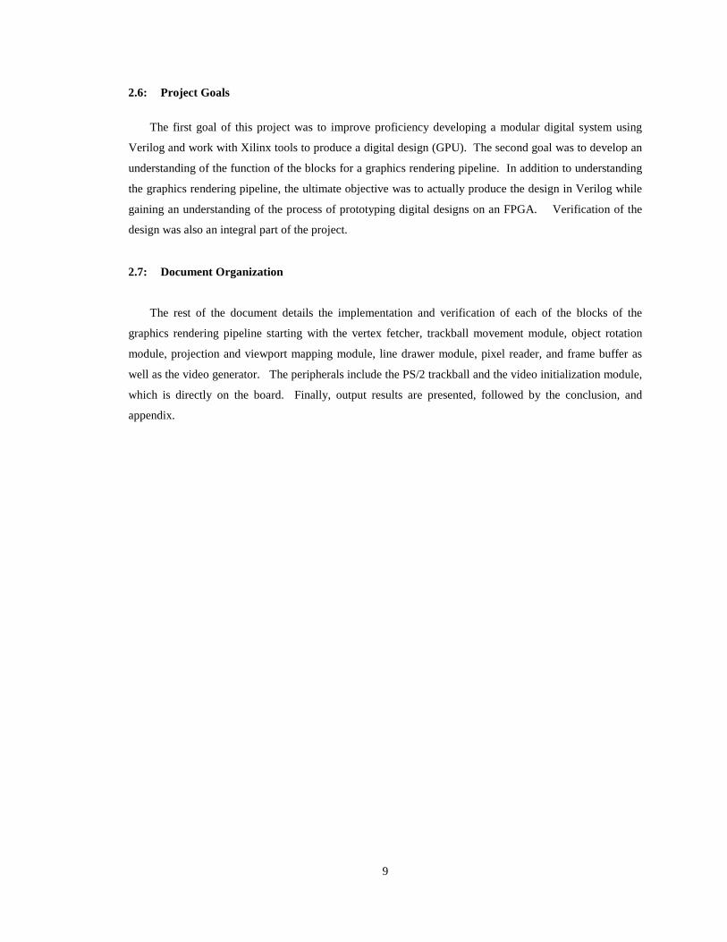
3.2: Trackball Movement Module
The implementation of the GPU began with the development and verification of the input interaction
block. The user interaction block is a PS/2 compatible scroll wheel mouse controller which was modified
slightly from Dr. Pong Chu’s Verilog example source as described in his text “FPGA prototyping by
Verilog examples Xilinx Spartan -3 version” [12]. The PS/2 controller core was designed using three state
machines. The first state machine describes the current state of the mouse packet transmission and
reception to/from the mouse. The main module containing the described state machine configuration
(packet controller created from scratch and the serial transmitter, and serial receiver used with slight
modification from Dr. Pong Chu’s example) has been consolidated and integrated with the packet
controller. The bit level state machines have been interconnected together structurally. They are depicted
as two separate modules in Figure 8. In the final design there was a problem using them separately because
of feedback errors in synthesis and as a result they were consolidated into one module to allow for design
logic partitioning during implementation.
Figure 8: Top Level Schematic of the Original PS/2 Tx/Rx Unit Shown as Separate Blocks
clk
ps2c
ps2d
reset
rx_en
dout(7:0)
rx_done_tick
din(7:0)
clk
reset
wr_ps2
state_reg(2:0)
ps2d
tx_done_tick
tx_idle
ps2c
clk
ps2c
ps2d
reset
din(7:0)
wr_ps2
dout(7:0)
rx_done_tick
state_reg(2:0)
tx_done_tick
12
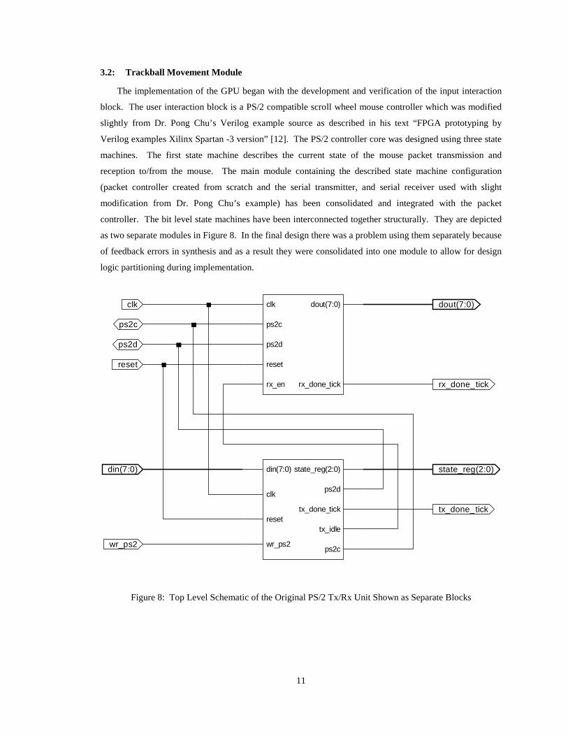
Mouse Protocol 3.2.1:
The mouse or trackball needed to be initialized before it can begin transmitting mouse movement to
the FPGA. In order to achieve successful initialization, a top level controller has been created which is
capable of running the low level serial transmit receive state machines and allow them to send data back
and forth between the host FPGA and the mouse peripheral. To understand the PS/2 protocol it is
important to review the main steps involved in transmission or reception of data. The PS/2 is a serial bi-
directional protocol used to interface keyboards and mice to a host processor. The FPGA in these
waveforms is the device which has control over the data line and must send a request to initialize the mouse
for receiving displacement information. To request control of the data line the host pulls clock low and
then data low and then releases clock. The PS/2 mouse oscillates the clock in order to transmit or receive
packets of data. The protocol is depicted in Figure 9 and Figure 10.
Figure 9: Device to Host Communication (Data Bit Read on Rising Edge of Clock) [13]
Figure 10: Host to Device Communication (Data Bit Read on Falling Edge of Clock) [13]
1. Host brings the clock line low for at least 100 microseconds 2. Bring the data line low 3. Release the clock line 4. Wait for the device to bring the clock line low 5. Set/reset the data line to send the first data bit 6. Wait for the device to bring clock high 7. Wait for the device to bring clock low 8. Repeat steps 5-7 for the other seven data bits and the parity bit 9. Release the data line 10. Wait for the device to bring data low 11. Wait for the device to bring clock low 12. Wait for the device to release data and clock
Figure 11: PS/2 Communication Protocol [14]
Start D0 D1 D2 D3 D4 D5 D6 D7 Parity Stop
Clock
Data
Start D0 D1 D2 D3 D4 D5 D6 D7 Parity Stop
Clock
Data
Ack
13
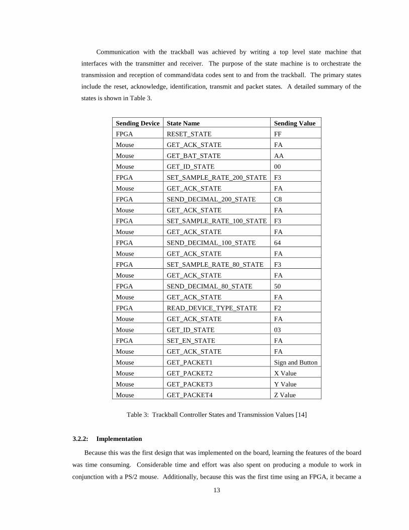
Communication with the trackball was achieved by writing a top level state machine that
interfaces with the transmitter and receiver. The purpose of the state machine is to orchestrate the
transmission and reception of command/data codes sent to and from the trackball. The primary states
include the reset, acknowledge, identification, transmit and packet states. A detailed summary of the
states is shown in Table 3.
Sending Device State Name Sending Value FPGA RESET_STATE FF Mouse GET_ACK_STATE FA Mouse GET_BAT_STATE AA Mouse GET_ID_STATE 00 FPGA SET_SAMPLE_RATE_200_STATE F3 Mouse GET_ACK_STATE FA FPGA SEND_DECIMAL_200_STATE C8 Mouse GET_ACK_STATE FA FPGA SET_SAMPLE_RATE_100_STATE F3 Mouse GET_ACK_STATE FA FPGA SEND_DECIMAL_100_STATE 64 Mouse GET_ACK_STATE FA FPGA SET_SAMPLE_RATE_80_STATE F3 Mouse GET_ACK_STATE FA FPGA SEND_DECIMAL_80_STATE 50 Mouse GET_ACK_STATE FA FPGA READ_DEVICE_TYPE_STATE F2 Mouse GET_ACK_STATE FA Mouse GET_ID_STATE 03 FPGA SET_EN_STATE FA Mouse GET_ACK_STATE FA Mouse GET_PACKET1 Sign and Button Mouse GET_PACKET2 X Value Mouse GET_PACKET3 Y Value Mouse GET_PACKET4 Z Value
Table 3: Trackball Controller States and Transmission Values [14]
Implementation 3.2.2:
Because this was the first design that was implemented on the board, learning the features of the board
was time consuming. Considerable time and effort was also spent on producing a module to work in
conjunction with a PS/2 mouse. Additionally, because this was the first time using an FPGA, it became a

14
challenge to overcome learning curve to develop further designs. Moreover, it became clear in hindsight
that the main problem in developing this module was in mixing behavioral descriptions with module
instantiations and not dividing the combinational logic into separate functions. This approach proved very
difficult to debug. In fact, the generated schematic showed a great deal of overlap of gate level components
and hierarchical blocks which took more time to troubleshoot than expected. The lesson learned from this
block was not to mix module instantiations and behavioral code in one block for synthesis. This caused
difficulties during block integration and added more time to debug the design. Although the mouse was
working, it became clear that there was a need to segregate all components using modules and functions.
The primary means for debugging the mouse module was to observe its direction of motion using the
on-board LEDs. Before the motion counters were able to be received, the first step was to verify that the
mouse was in streaming (transmitting) mode. Streaming mode means that the mouse delivers packets to the
FPGA represented as 9 bit signed 2’s compliment values for X and Y, and 4 bit 2’s complement Z values.
Figure 12 summarizes the packet level protocol for a PS/2 mouse. The packets are transmitted to the host
(FPGA) during streaming mode.
Bit 7 Bit 6 Bit 5 Bit 4 Bit 3 Bit 2 Bit 1 Bit 0
Byte 1 Y overflow X overflow Y sign bit X sign bit Always 1 Middle Btn Right Btn Left Btn
Byte 2 X Movement
Byte 3 Y Movement
Byte 4 Z Movement
Figure 12: Depiction of 4 byte packets transmitted from mouse to host FPGA [14]
The initial goal of the mouse module stage (Block A) was to produce a cursor capable of being
displayed on a monitor, and this goal has been achieved. Through many trial-and-error loops, the first
cursor was displayed on the screen. The next step was to move the cursor using a standard Microsoft PS/2
mouse. Majority of the learning took place in experimenting with the board features and implementing
simpler modules on the FPGA. Eventually a trackball was purchased to give the user the ease of traversing
three orthogonal axes of movement.
The mouse packet controller state machine was created incrementally. First, the state and transmission
values were used to create parameters in Verilog, along with a list of parameterized command values sent
to and from the FPGA.
After setting out all of the parameters, the next step was to write the transition conditions and develop
the state machine in Verilog. When the mouse is powered on the first step is to wait until the controller

15
sends the reset mouse command. The mouse responds with a basic assurance test OK code of 0xAA at
which point it sends its standard identifier as a PS/2 mouse. The FPGA requests the mouse to stream
position information to the FPGA by sending an enable command. The mouse responds with an
acknowledge signal after the FPGAs command request (and after each command sent from the FPGA).
Finally, the FPGA receives packets 1 through 4 and then back to 1 so long as there is still power applied to
the mouse. The FPGA’s next job is to decode the position into an angle, displacement or scaling value and
apply it to the object that is loaded into the FPGA. Figure 13 depicts a simplified diagram of the described
packet level protocol.
Figure 13: Simplified Mouse Initialization/Streaming Controller State Machine
Verification 3.2.3:
After the module was written, the next step was to verify its functionality. This proved to be the most
time consuming activity among all of the modules primarily because there were logic errors present in the
design and because this was the first time working with an FPGA board. Many times the logic was stuck
at a particular state and only by outputting the state to the board LEDs was the state fault resolved. The
first step to verify the design was to create a test fixture and run a behavioral simulation on the mouse. The
test fixture sent responses to the DUV (design under verification) and function as a simulated mouse. The
waves included the names of the states along with the bi-directional lines which were optionally pulled
high using a pull-up resistor in Verilog. A depiction of the LED arrangement on board the V5LX110T
IDLE RESET Reset BASIC
ASSURE TEST
GET MOUSE
ID
SET SAMPLE
RATE ENABLE
PACKET 1
PACKET 2
PACKET 3
PACKET 4
Transmit Done
Basic Assurance
OK
16
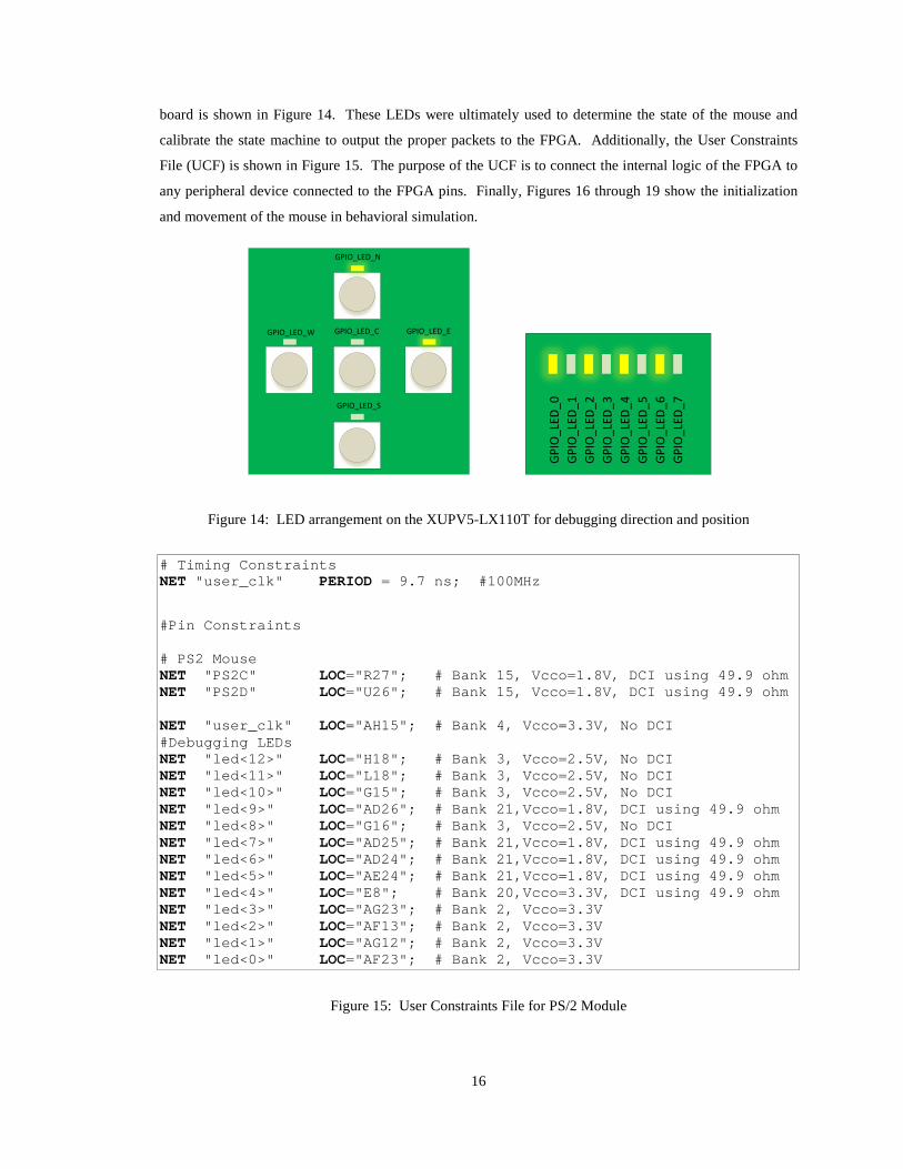
board is shown in Figure 14. These LEDs were ultimately used to determine the state of the mouse and
calibrate the state machine to output the proper packets to the FPGA. Additionally, the User Constraints
File (UCF) is shown in Figure 15. The purpose of the UCF is to connect the internal logic of the FPGA to
any peripheral device connected to the FPGA pins. Finally, Figures 16 through 19 show the initialization
and movement of the mouse in behavioral simulation.
Figure 14: LED arrangement on the XUPV5-LX110T for debugging direction and position
# Timing Constraints NET "user_clk" PERIOD = 9.7 ns; #100MHz
#Pin Constraints # PS2 Mouse NET "PS2C" LOC="R27"; # Bank 15, Vcco=1.8V, DCI using 49.9 ohm NET "PS2D" LOC="U26"; # Bank 15, Vcco=1.8V, DCI using 49.9 ohm NET "user_clk" LOC="AH15"; # Bank 4, Vcco=3.3V, No DCI #Debugging LEDs NET "led<12>" LOC="H18"; # Bank 3, Vcco=2.5V, No DCI NET "led<11>" LOC="L18"; # Bank 3, Vcco=2.5V, No DCI NET "led<10>" LOC="G15"; # Bank 3, Vcco=2.5V, No DCI NET "led<9>" LOC="AD26"; # Bank 21,Vcco=1.8V, DCI using 49.9 ohm NET "led<8>" LOC="G16"; # Bank 3, Vcco=2.5V, No DCI NET "led<7>" LOC="AD25"; # Bank 21,Vcco=1.8V, DCI using 49.9 ohm NET "led<6>" LOC="AD24"; # Bank 21,Vcco=1.8V, DCI using 49.9 ohm NET "led<5>" LOC="AE24"; # Bank 21,Vcco=1.8V, DCI using 49.9 ohm NET "led<4>" LOC="E8"; # Bank 20,Vcco=3.3V, DCI using 49.9 ohm NET "led<3>" LOC="AG23"; # Bank 2, Vcco=3.3V NET "led<2>" LOC="AF13"; # Bank 2, Vcco=3.3V NET "led<1>" LOC="AG12"; # Bank 2, Vcco=3.3V NET "led<0>" LOC="AF23"; # Bank 2, Vcco=3.3V
Figure 15: User Constraints File for PS/2 Module
GPIO_LED_C GPIO_LED_E
GPIO_LED_N
GPIO_LED_W
GPIO_LED_S
GPIO
_LED
_0GP
IO_L
ED_1
GPIO
_LED
_2GP
IO_L
ED_3
GPIO
_LED
_4GP
IO_L
ED_5
GPIO
_LED
_6GP
IO_L
ED_7

17
Figure 16: Mouse Initialization Behavioral Simulation
0000
0000
1111
1111
1100
1111
0001
0011
1100
1111
0010
0110
1100
1111
0000
1010
0100
1111
0010
1111
0000
100
010
0001
100
100
0010
100
010
0100
000
010
0011
000
010
0100
100
010
0011
100
010
0101
000
010
0101
100
010
0010
001
100
0001
001
101
250
250
1111
1010
1010
1010
0000
0000
1111
1010
0000
0011
1111
1010
0000
1000
RE
SE
T_S
TATE
GET
_AC
K_ST
ATE
GE
T_BA
T_ST
ATE
GE
T_ID
_STA
TES
ET_
SAM
PLE
_R
ATE_
200_
STA
TEG
ET_A
CK_
STA
TESE
ND_
DECI
MAL
_200
_S
TATE
GE
T_AC
K_ST
ATE
SE
T_S
AMP
LE_R
ATE
_100
_ST
ATE
GET
_AC
K_ST
ATE
SEN
D_D
ECIM
AL_
100_
STAT
EG
ET_A
CK_S
TATE
SET
_SAM
PLE
_RAT
E_80
_STA
TEG
ET_A
CK_
STA
TESE
ND_
DEC
IMAL
_80_
STAT
EG
ET_A
CK_
STA
TER
EAD
_DEV
ICE_
TYPE
_STA
TEG
ET_
ACK_
STAT
EG
ET_I
D_ST
ATE
SE
T_E
N_S
TATE
GE
T_AC
K_ST
ATE
GET
_PA
CKE
T1
CO
NTR
OLL
ER_S
END
ING
CO
NTR
OLL
ER_R
ECEI
VIN
GC
ON
TRO
LLE
R_SE
ND
ING
CO
NTR
OLL
ER
_RE
CEI
VING
CO
NTR
OLL
ER_S
EN
DIN
GC
ON
TROL
LER
_RE
CEI
VIN
GC
ON
TRO
LLER
_SE
NDI
NG
CO
NTR
OLL
ER_R
EC
EIV
ING
CO
NTR
OLL
ER_S
EN
DING
CO
NTR
OLL
ER_R
EC
EIV
ING
CO
NTR
OLL
ER_
SEN
DIN
GC
ONT
RO
LLE
R_RE
CEI
VIN
GC
ON
TRO
LLE
R_SE
ND
ING
CO
NTR
OLL
ER
_RE
CE
IVIN
GC
ON
TRO
LLER
_SEN
DIN
GC
ON
TRO
LLE
R_R
EC
EIV
ING
CO
NTR
OLL
ER_S
EN
DIN
GC
ON
TRO
LLE
R_R
EC
EIV
ING
REQ
UE
STTO
SEN
D
DAT
AID
LER
EQU
EST
TO
SEN
D
DAT
AID
LER
EQ
UEST
TOS
END
DAT
AID
LER
EQ
UES
TTO
SEN
D
DAT
AID
LERE
QUE
ST
TOS
END
DAT
AID
LER
EQU
EST
TOS
END
DAT
AID
LER
EQU
EST
TO
SEN
D
DAT
AID
LER
EQ
UEST
TOS
END
DAT
AID
LER
EQ
UEST
TOS
END
DAT
AID
LE
0000
000
001
0001
000
011
0010
000
101
0011
000
111
0100
001
001
001
011
000
001
011
000
001
011
000
001
011
000
001
011
000
001
011
000
001
011
000
001
011
000
001
011
000
0000
0000
0xxx
x
/mou
se_x
yz_t
b/PS
2C_g
en
/mou
se_x
yz_t
b/PS
2D_g
en
/mou
se_x
yz_t
b/PS
2D_e
n
/mou
se_x
yz_t
b/D
ATA_
in00
0000
0011
1111
1111
0011
1100
0100
1111
0011
1100
1001
1011
0011
1100
0010
1001
0011
1100
1011
11
/mou
se_x
yz_t
b/Pa
rity
/mou
se_x
yz_t
b/St
op
/mou
se_x
yz_t
b/St
art
/mou
se_x
yz_t
b/st
ate
0000
100
010
0001
100
100
0010
100
010
0100
000
010
0011
000
010
0100
100
010
0011
100
010
0101
000
010
0101
100
010
0010
001
100
0001
001
101
/mou
se_x
yz_t
b/xP
ositi
on25
0
/mou
se_x
yz_t
b/yP
ositi
on25
0
/mou
se_x
yz_t
b/PS
2D
/mou
se_x
yz_t
b/D
ata_
out
1111
1010
1010
1010
0000
0000
1111
1010
0000
0011
1111
1010
0000
1000
/mou
se_x
yz_t
b/st
ate_
deco
deR
ES
ET_
STA
TEG
ET_A
CK_
STAT
EG
ET_
BAT_
STAT
EG
ET_
ID_S
TATE
SET
_S
AMP
LE_
RAT
E_20
0_S
TATE
GET
_AC
K_S
TATE
SEN
D_DE
CIM
AL_2
00_
STA
TEG
ET_
ACK_
STAT
ES
ET_
SAM
PLE
_RAT
E_1
00_
STA
TEG
ET_A
CK_
STAT
ESE
ND
_DEC
IMA
L_10
0_ST
ATE
GET
_ACK
_STA
TESE
T_S
AMPL
E_R
ATE_
80_S
TATE
GET
_AC
K_S
TATE
SEN
D_D
ECIM
AL_8
0_ST
ATE
GET
_AC
K_S
TATE
REA
D_D
EVIC
E_TY
PE_S
TATE
GE
T_AC
K_ST
ATE
GET
_ID_
STAT
ES
ET_
EN
_STA
TEG
ET_
ACK_
STAT
EG
ET_P
ACK
ET1
/mou
se_x
yz_t
b/se
nd_r
ecei
ve_s
tate
CO
NTR
OLL
ER_S
END
ING
CO
NTR
OLL
ER_R
ECEI
VIN
GC
ON
TRO
LLE
R_SE
ND
ING
CO
NTR
OLL
ER
_RE
CEI
VING
CO
NTR
OLL
ER_S
EN
DIN
GC
ON
TROL
LER
_RE
CEI
VIN
GC
ON
TRO
LLER
_SE
NDI
NG
CO
NTR
OLL
ER_R
EC
EIV
ING
CO
NTR
OLL
ER_S
EN
DING
CO
NTR
OLL
ER_R
EC
EIV
ING
CO
NTR
OLL
ER_
SEN
DIN
GC
ONT
RO
LLE
R_RE
CEI
VIN
GC
ON
TRO
LLE
R_SE
ND
ING
CO
NTR
OLL
ER
_RE
CE
IVIN
GC
ON
TRO
LLER
_SEN
DIN
GC
ON
TRO
LLE
R_R
EC
EIV
ING
CO
NTR
OLL
ER_S
EN
DIN
GC
ON
TRO
LLE
R_R
EC
EIV
ING
/mou
se_x
yz_t
b/tx
_sta
te_d
ecod
eRE
QU
EST
TOS
END
DAT
AID
LER
EQU
EST
TO
SEN
D
DAT
AID
LER
EQ
UEST
TOS
END
DAT
AID
LER
EQ
UES
TTO
SEN
D
DAT
AID
LERE
QUE
ST
TOS
END
DAT
AID
LER
EQU
EST
TOS
END
DAT
AID
LER
EQU
EST
TO
SEN
D
DAT
AID
LER
EQ
UEST
TOS
END
DAT
AID
LER
EQ
UEST
TOS
END
DAT
AID
LE
/mou
se_x
yz_t
b/st
ream
ingM
ode
/mou
se_x
yz_t
b/re
ques
tToS
end
/mou
se_x
yz_t
b/se
tInde
x00
000
0000
100
010
0001
100
100
0010
100
110
0011
101
000
0100
1
/mou
se_x
yz_t
b/st
ate_
reg
001
011
000
001
011
000
001
011
000
001
011
000
001
011
000
001
011
000
001
011
000
001
011
000
001
011
000
/mou
se_x
yz_t
b/le
d00
0000
000x
xxx
/glb
l/GSR
04
us8
us12
us
Entit
y:m
ouse
_xyz
_tb
Arch
itect
ure:
Dat
e:Th
u Fe
b 17
2:4
3:23
PM
Pac
ific
Stan
dard
Tim
e 20
11
Row
: 1 P
age:
1

18
Figure 17: Mouse Initialization (Part 2) Behavioral Simulation
0010
0110
1100
1111
0000
1010
0100
1111
0011
100
010
0110
100
010
1000
100
010
0010
0
307
205
0000
0000
000
0000
0000
000
0000
0000
000
1111
1010
0000
0011
SET_
SAM
PLE_
RAT
E_80
_STA
TEG
ET_
ACK_
STA
TESE
ND
_DEC
IMAL
_80_
STAT
EG
ET_
ACK_
STA
TER
EAD
_DEV
ICE_
TYPE
_STA
TEG
ET_A
CK_
STAT
EG
ET_I
D_S
TATE
CO
NTR
OLL
ER
_SE
ND
ING
CO
NTR
OLL
ER
_RE
CE
IVIN
GC
ON
TRO
LLER
_SEN
DIN
GC
ON
TRO
LLE
R_R
EC
EIV
ING
CO
NTR
OLL
ER_S
END
ING
CO
NTR
OLL
ER_R
ECEI
VIN
G
REQ
UE
STT
OS
END
DAT
AST
OP
IDLE
RE
QU
EST
TO S
EN
DD
ATA
STOP
IDLE
RE
QU
EST
TO S
EN
DD
ATA
STO
P
IDLE
0010
100
110
0011
1
001
011
100
000
001
011
100
000
001
011
100
000
/mou
se_t
b/PS
2C_e
n
/mou
se_t
b/PS
2D_e
n
/mou
se_t
b/DA
TA_i
n00
1001
1011
0011
1100
0010
1001
0011
11
/mou
se_t
b/Pa
rity
/mou
se_t
b/st
ate
0011
100
010
0110
100
010
1000
100
010
0010
0
/mou
se_t
b/xP
ositi
on30
7
/mou
se_t
b/yP
ositi
on20
5
/mou
se_t
b/PS
2D
/mou
se_t
b/PS
2C
/mou
se_t
b/SD
PS00
0000
0000
000
0000
0000
000
0000
0000
0
/mou
se_t
b/D
ata_
out
1111
1010
0000
0011
/mou
se_t
b/st
ate_
deco
deSE
T_SA
MPL
E_R
ATE_
80_S
TATE
GE
T_AC
K_S
TATE
SEN
D_D
ECIM
AL_8
0_ST
ATE
GE
T_AC
K_S
TATE
REA
D_D
EVIC
E_TY
PE_S
TATE
GET
_AC
K_ST
ATE
GET
_ID
_STA
TE
/mou
se_t
b/se
nd_r
ecei
ve_s
tate
CO
NTR
OLL
ER
_SE
ND
ING
CO
NTR
OLL
ER
_RE
CE
IVIN
GC
ON
TRO
LLER
_SEN
DIN
GC
ON
TRO
LLE
R_R
EC
EIV
ING
CO
NTR
OLL
ER_S
END
ING
CO
NTR
OLL
ER_R
ECEI
VIN
G
/mou
se_t
b/tx
_sta
te_d
ecod
eR
EQU
EST
TO
SEN
D
DAT
AST
OP
IDLE
RE
QU
EST
TO S
EN
DD
ATA
STOP
IDLE
RE
QU
EST
TO S
EN
DD
ATA
STO
P
IDLE
/mou
se_t
b/st
ream
ingM
ode
/mou
se_t
b/re
ques
tToSe
nd
/mou
se_t
b/se
tInde
x00
101
0011
000
111
/mou
se_t
b/st
ate_
reg
001
011
100
000
001
011
100
000
001
011
100
000
9 m
s10
ms
11m
s12
ms
13 m
s
Entit
y:m
ouse
_tb
Arch
itect
ure:
Dat
e: F
ri Ja
n 14
5:1
3:34
PM
Pac
ific
Stan
dard
Tim
e 20
11
Row
: 1 P
age:
1

19
Figure 18: Streaming Packets from PS2 Mouse (Y Movement)
0010
1111
307
203
202
201
200
199
198
197
196
195
194
193
192
191
190
189
188
187
186
185
186
187
188
189
190
191
192
193
194
195
196
197
198
199
200
201
202
203
204
205
CO
NTR
OLL
ER_R
ECEI
VIN
G
IDLE
1000
1
000
/mou
se_t
b/PS
2D_e
n
/mou
se_t
b/DA
TA_i
n00
1011
11
/mou
se_t
b/Pa
rity
/mou
se_t
b/st
ate
/mou
se_t
b/xP
ositi
on30
7
/mou
se_t
b/yP
ositi
on20
320
220
120
019
919
819
719
619
519
419
319
219
119
018
918
818
718
618
518
618
718
818
919
019
119
219
319
419
519
619
719
819
920
020
120
220
320
420
5
/mou
se_t
b/D
ata_
out
/mou
se_t
b/st
ate_
deco
de
/mou
se_t
b/se
nd_r
ecei
ve_s
tate
CO
NTR
OLL
ER_R
ECEI
VIN
G
/mou
se_t
b/tx
_sta
te_d
ecod
eID
LE
/mou
se_t
b/st
ream
ingM
ode
/mou
se_t
b/re
ques
tToSe
nd
/mou
se_t
b/se
tInde
x10
001
/mou
se_t
b/st
ate_
reg
000
40 m
s60
ms
80 m
s10
0 m
s
Entit
y:m
ouse
_tb
Arch
itect
ure:
Dat
e: F
ri Ja
n 14
5:2
6:43
PM
Pac
ific
Stan
dard
Tim
e 20
11
Row
: 1 P
age:
1

20
Figure 19: Streaming Packets from PS2 Mouse (X Movement)
0010
1111
308
309
310
311
312
313
314
315
316
317
318
319
320
321
322
323
324
325
326
327
326
325
324
323
322
321
320
319
318
317
316
315
314
313
312
311
310
309
308
307
205
0000
000
0
CO
NTR
OLL
ER_R
ECEI
VIN
G
IDLE
1000
1
000
/mou
se_t
b/PS
2D_e
n
/mou
se_t
b/DA
TA_i
n00
1011
11
/mou
se_t
b/Pa
rity
/mou
se_t
b/st
ate
/mou
se_t
b/xP
ositi
on30
830
931
031
131
231
331
431
531
631
731
831
932
032
132
232
332
432
532
632
732
632
532
432
332
232
132
031
931
831
731
631
531
431
331
231
131
030
930
830
7
/mou
se_t
b/yP
ositi
on20
5
/mou
se_t
b/D
ata_
out
0000
000
0
/mou
se_t
b/st
ate_
deco
de
/mou
se_t
b/se
nd_r
ecei
ve_s
tate
CO
NTR
OLL
ER_R
ECEI
VIN
G
/mou
se_t
b/tx
_sta
te_d
ecod
eID
LE
/mou
se_t
b/st
ream
ingM
ode
/mou
se_t
b/re
ques
tToSe
nd
/mou
se_t
b/se
tInde
x10
001
/mou
se_t
b/st
ate_
reg
000
120
ms
140
ms
160
ms
180
ms
200
ms
Ent
ity:m
ouse
_tb
Arc
hite
ctur
e: D
ate:
Fri
Jan
14 5
:35:
52 P
M P
acifi
c S
tand
ard
Tim
e 20
11
Row
: 1 P
age:
1

21
3.3: Vertex Fetcher
The next module in the pipeline is the vertex fetcher. The purpose of the vertex fetcher is to retrieve
vertices from the Block RAMs where the vertices are stored. As mentioned in Chapter 2, the file format
used is OFF, where coordinate values are represented as base 10 decimal fractions. Using a conversion
script4, the OFF vertices were converted into a binary look-up table which was suited for processing on the
FPGA. Prior to using an external data set, a hard-coded state machine with vertex coordinates was used
and the module was called the shape generator. It consisted of four states, one state per each of the four
lines, and it was used to generate a four-line object such as an “x” where lines met in the center of the
screen and the center was controlled by the mouse trackball. The state machine controller block diagram
is shown in Figure 20.
Figure 20: Vertex Fetcher Controller Block Diagram (Inputs on Left, Outputs on Right)
As its name suggests, the vertex streamer acquires points from the vertex memory (FPGA dual-port
block rams) and feeds them into the graphics pipeline. They can also be manipulated using the rotation
module which, one by one, alters the coordinates fetched from memory. The original contents of memory
remain un-altered. The vertex streamer is a revision from the original shape generation module which
consists of a statically hard-coded object in a state machine (one state per edge of the object). The state
machine is depicted in Figure 21. It consists of six depicted states - reset, idle, line1, line2, line3, and line4.
Not shown in the state diagram is the line clearing states which essentially draw the background color
to the frame buffer. Though inefficient in hindsight, hard coding the lines, proved to be a quick way to
produce a four-lined object using a small amount of memory content and only hard-coded vertex values.
Before each draw cycle it was important to clear the screen by removing the lines. More detail about the
video generation and line drawing process is discussed towards the end of Chapter 3. Also, the creation of
4Conversion script modified from http://www.easysurf.cc/cnver17.htm#b10tob2
clearDone clk lineUnderProcess mouseStreaming rasterizerDone reset triangleProcessing~reg0 coordNumUnderProcessReg3[2..0] lineNumberUnderProcess[2..0] rotationAmount[9..0] rotationAxis[1..0] trian g leNumber [ 9..0 ]
SHAPE_DONE WRITE_PIXELS_TO_FRAME_BUFFER
PREPARE_TO_WRITE_PIXELS PROJECTING_COORDINATES
FETCH_NEW_VERTICES FETCH_NEW_TRIANGLE
coordProcessState

22
the line on the screen produced artifacts when the FPGA was reset which were cleared when a new line was
drawn over the original line in the buffer.
The vertex fetcher was developed in conjunction with the projection module is covered towards the
end of this Chapter. It fetches data concurrently while the FPGA initializes the mouse and receives
packets. Below are the state machine diagrams with and without clear states.
Figure 21: Original Static Pyramid – Shape Generator State Machine without clear states In Figure 21 the rasterizerDone transition condition was shown between Line 1 State and Line 2 State,
as well as Line 4 State and Idle State. It is not shown between Line2 and Line 3 State nor is it shown
between Line 3 State and Line 4 State. Figure 22 depicts the full state machine with the clear states. Note
that the state transition equations are not shown in the figure below.
Figure 22: Original Static Four Line Shape Generator State Machine with Clear States
InitializeValues
RESET
Wait for done signalFrom
rasterizer
IDLE
Assign Line 1
Coords
LINE1
AssignLine 2
Coords
LINE2
Assign Line 3
Coords
LINE3
Assign Line 4
Coords
LINE4
rast
erize
rDon
e
rasterizerDone
Cond: (drawTriangle)
Cond: (rasterizerDone)
Cond: (rasterizerDone) Cond: (rasterizerDone)
Cond: (rasterizerDone)
Cond: (rasterizerDone)
Cond: (rasterizerDone) Cond: (rasterizerDone) Cond: (~reset)
Cond: (rasterizerDone)
Cond: && (mouse_moving&(xIntersectCoord!=xPosLast| Cond: 1
IDLE_STATE
CLEAR_LINE_1
RASTERIZE_LINE_1
CLEAR_LINE_2
CLEAR_LINE_3
CLEAR_LINE_4 RASTERIZE_LINE_2
RASTERIZE_LINE_3
RASTERIZE_LINE_4
SHAPE_DONE

23
Once the four line generator was created, the next step was to create a new method for generalizing the
state machine for any dataset. This meant that the vertex fetcher was capable of handling any amount of
data within limits specified in the parameter definitions of the vertex fetcher module. The vertex fetcher
takes triangles from the dataset and fetches all the vertices. It is also responsible for coordinating the
projection of the coordinates and writing the pixels to the frame buffer. Once the triangle is done, the state
machine receives a new triangle from the dataset and fetches all coordinates. This processing repeats until
the shape is finally done at which point the object is finished. A mouse movement triggers a new
coordinate to be drawn. The way a new set of coordinates are streamed through the pipeline is when the
user moves the mouse. The state machine shown is shown in Figure 23.
Figure 23: Vertex Fetcher State Machine
Cond: (((lineNumberUnderProcess<3) && (lineUnderProcess==1)) && (rasterizerDone))
Cond: ((!(lineNumberUnderProcess<3) && (lineNumberUnderProcess==3&rasterizerDone ... && (objectFinished))
Cond: ((!(lineNumberUnderProcess<3) && (lineNumberUnderProcess==3&rasterizerDone ... && !(objectFinished))
Cond: 1
Cond: !(coordNumUnderProcessReg<4) Cond: 1
Cond: 1
Cond: (~reset)
FETCH_NEW_TRIANGLE
FETCH_NEW_VERTICES
PROJECTING_COORDINATES
PREPARE_TO_WRITE_PIXELS
WRITE_PIXELS_TO_FRAME_BUFFER
SHAPE_DONE

24
3.4: Coordinate Rotator
The purpose of the coordinate rotator is to take unaltered (no change from original dataset) coordinates
and perform the rotation operation on each coordinate, one at a time. The method of rotation is done by
adding two operands or subtracting two operands. Each of the operands that are added or subtracted are
single dimensional rotations (the operands of the add/subtract) values. When added or subtracted together
the rotation forms a 2D rotation. To achieve 2D rotation, simply repeat the process for the next orthogonal
pair of axes that are not on the rotation axis. Keep the axis of rotation unaltered. This operation completes
the 3D rotation about a single axis for an arbitrary rotation. The significance of keeping rotation axes
separate for composite operations is that they can be performed independent of the other rotations. If a
rotation operation rotates 30 degrees across the x axis, followed by 30 degrees on either y or z axis the
operations do not interfere. Rotation in 3D is a composite operation of arithmetic (addition/subtraction of
2D rotations) and multiplies and trigonometric coefficient computations (1D rotation using a sine/cosine
ROM). To compose 3D rotations from one axis to another axis, take the first axis and perform the
rotation then store the angle of rotation to perform the second rotation. This method of combining rotations
works well with a mouse interface which outputs each axis of movement on successive bursts. Figure 24
depicts the block diagram of the coordinate rotator for a rotation about the x axis.
Figure 24: Coordinate Rotator Block Diagram
Mathematics of Rotation 3.4.1:
When an object is rotated about any axis, the values of all points on the axis remain constant while the
other two axis values change. If an object were to be rotated about the z axis, the x, and y values change
according to the rotation angle theta and its original value phi. Equation 3.1 shows the mathematics for a
rotation about the z axis using the sum of angles formula in trigonometry. Phi (𝜙) is the original angle from
the reference axis, theta (𝜃) is the angle of rotation, and rho (𝜌) is the radius. Once the equations are
determined, then the next step is to insert the components into the rotation matrix. Equation 1 presents 2D
SIN/COSROM
cos(ϴ)
cos(ϴ)
sin(ϴ)
sin(ϴ)
y
y
z
z
y cos(ϴ)
z cos(ϴ)
y sin(ϴ)
z sin(ϴ)
zRotated = z cos(ϴ) + y sin(ϴ)
yRotated = y cos(ϴ) – z sin(ϴ)
Angle Address (n)
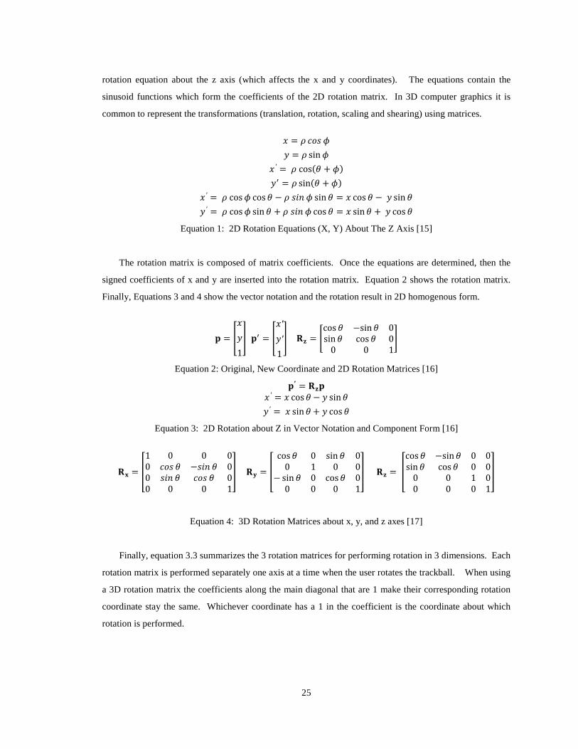
25
rotation equation about the z axis (which affects the x and y coordinates). The equations contain the
sinusoid functions which form the coefficients of the 2D rotation matrix. In 3D computer graphics it is
common to represent the transformations (translation, rotation, scaling and shearing) using matrices.
𝑥 = 𝜌 𝑐𝑜𝑠 𝜙𝑦 = 𝜌 sin𝜙
𝑥 ′ = 𝜌 cos(𝜃 + 𝜙)𝑦′ = 𝜌 sin(𝜃 + 𝜙)
𝑥 ′ = 𝜌 cos𝜙 cos𝜃 − 𝜌 𝑠𝑖𝑛 𝜙 sin𝜃 = 𝑥 cos 𝜃 − 𝑦 sin 𝜃𝑦′ = 𝜌 cos𝜙 sin 𝜃 + 𝜌 𝑠𝑖𝑛 𝜙 cos 𝜃 = 𝑥 sin𝜃 + 𝑦 cos 𝜃
Equation 1: 2D Rotation Equations (X, Y) About The Z Axis [15]
The rotation matrix is composed of matrix coefficients. Once the equations are determined, then the
signed coefficients of x and y are inserted into the rotation matrix. Equation 2 shows the rotation matrix.
Finally, Equations 3 and 4 show the vector notation and the rotation result in 2D homogenous form.
𝐩 = �𝑥𝑦1� 𝐩′ = �
𝑥′𝑦′1� 𝐑𝐳 = �
cos 𝜃 −sin𝜃 0sin𝜃 cos 𝜃 0
0 0 1�
Equation 2: Original, New Coordinate and 2D Rotation Matrices [16]
𝐩′ = 𝐑𝐳𝐩 𝑥 ′ = 𝑥 cos𝜃 − 𝑦 sin𝜃𝑦′ = 𝑥 sin𝜃+ 𝑦 cos 𝜃
Equation 3: 2D Rotation about Z in Vector Notation and Component Form [16]
𝐑𝐱 = �
1 0 0 00 𝑐𝑜𝑠 𝜃 −𝑠𝑖𝑛 𝜃 00 𝑠𝑖𝑛 𝜃 𝑐𝑜𝑠 𝜃 00 0 0 1
� 𝐑𝐲 = �
cos 𝜃 0 sin 𝜃 00 1 0 0
− sin 𝜃 0 cos𝜃 00 0 0 1
� 𝐑𝐳 = �
cos 𝜃 −sin𝜃 0 0sin𝜃 cos 𝜃 0 0
0 0 1 00 0 0 1
�
Equation 4: 3D Rotation Matrices about x, y, and z axes [17]
Finally, equation 3.3 summarizes the 3 rotation matrices for performing rotation in 3 dimensions. Each
rotation matrix is performed separately one axis at a time when the user rotates the trackball. When using
a 3D rotation matrix the coefficients along the main diagonal that are 1 make their corresponding rotation
coordinate stay the same. Whichever coordinate has a 1 in the coefficient is the coordinate about which
rotation is performed.
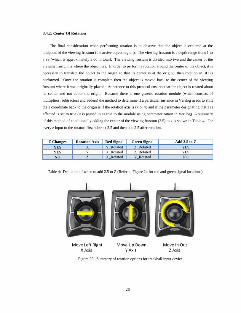
26
Center Of Rotation 3.4.2:
The final consideration when performing rotation is to observe that the object is centered at the
midpoint of the viewing frustum (the active object region). The viewing frustum is a depth range from 1 to
3.99 (which is approximately 3.00 in total). The viewing frustum is divided into two and the center of the
viewing frustum is where the object lies. In order to perform a rotation around the center of the object, it is
necessary to translate the object to the origin so that its center is at the origin; then rotation in 3D is
performed. Once the rotation is complete then the object is moved back to the center of the viewing
frustum where it was originally placed. Adherence to this protocol ensures that the object is rotated about
its center and not about the origin. Because there is one generic rotation module (which consists of
multipliers, subtractors and adders) the method to determine if a particular instance in Verilog needs to shift
the z coordinate back to the origin is if the rotation axis is (x or y) and if the parameter designating that z is
affected is set to true (it is passed in as true to the module using parameterization in Verilog). A summary
of this method of conditionally adding the center of the viewing frustum (2.5) to z is shown in Table 4. For
every z input to the rotator, first subtract 2.5 and then add 2.5 after rotation.
Z Changes Rotation Axis Red Signal Green Signal Add 2.5 to Z YES X Y_Rotated Z_Rotated YES YES Y X_Rotated Z_Rotated YES NO Z X_Rotated Y_Rotated NO
Table 4: Depiction of when to add 2.5 to Z (Refer to Figure 24 for red and green signal locations)
Figure 25: Summary of rotation options for trackball input device
Move Left Right X Axis
Move Up Down Y Axis
Move In Out Z Axis
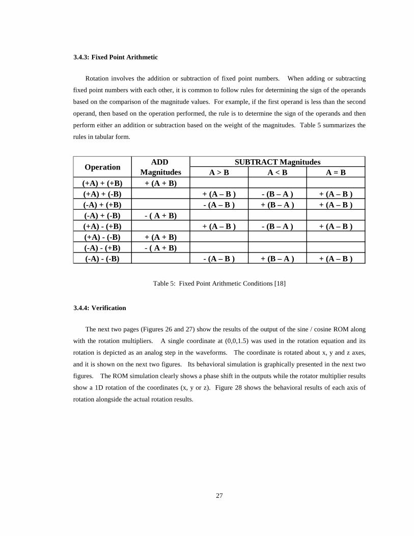
27
Fixed Point Arithmetic 3.4.3:
Rotation involves the addition or subtraction of fixed point numbers. When adding or subtracting
fixed point numbers with each other, it is common to follow rules for determining the sign of the operands
based on the comparison of the magnitude values. For example, if the first operand is less than the second
operand, then based on the operation performed, the rule is to determine the sign of the operands and then
perform either an addition or subtraction based on the weight of the magnitudes. Table 5 summarizes the
rules in tabular form.
Table 5: Fixed Point Arithmetic Conditions [18]
Verification 3.4.4:
The next two pages (Figures 26 and 27) show the results of the output of the sine / cosine ROM along
with the rotation multipliers. A single coordinate at (0,0,1.5) was used in the rotation equation and its
rotation is depicted as an analog step in the waveforms. The coordinate is rotated about x, y and z axes,
and it is shown on the next two figures. Its behavioral simulation is graphically presented in the next two
figures. The ROM simulation clearly shows a phase shift in the outputs while the rotator multiplier results
show a 1D rotation of the coordinates (x, y or z). Figure 28 shows the behavioral results of each axis of
rotation alongside the actual rotation results.
A > B A < B A = B(+A) + (+B) + (A + B)(+A) + (-B) + (A – B ) - (B – A ) + (A – B )(-A) + (+B) - (A – B ) + (B – A ) + (A – B )(-A) + (-B) - ( A + B)(+A) - (+B) + (A – B ) - (B – A ) + (A – B )(+A) - (-B) + (A + B)(-A) - (+B) - ( A + B)(-A) - (-B) - (A – B ) + (B – A ) + (A – B )
Operation SUBTRACT MagnitudesADD Magnitudes

28
Figure 26: Behavioral Simulation (Analog Step) of Sin/Cos ROM
/sin
CosR
OM
_TB_
v/co
sine
Fixe
d
/sin
CosR
OM
_TB_
v/si
neFi
xed
1000
0000
ps
2000
0000
ps
3000
0000
ps
4000
0000
ps
5000
0000
p
Entit
y:si
nCos
ROM
_TB_
vAr
chite
ctur
e:fa
stD
ate:
Sun
Aug
148:
32:1
9PM
Paci
ficD
aylig
htTi
me
2011
Row
:1
Page
:1

29
Figure 27: Behavioral Simulation (Analog Step) of Rotator Multipliers (Rotate x,y,z = 0,0,1.5 about each axis)
0 ps
5000
000
ps10
0000
00 p
s15
0000
00 p
s20
0000
00 p
s25
0000
00 p
s30
0000
00ps
/rot
ator
Mul
tiplie
rs_T
B/uu
t/co
ordi
nate
1Pro
duct
1Fix
ed
/rot
ator
Mul
tiplie
rs_T
B/uu
t/co
ordi
nate
1Pro
duct
2Fix
ed
/rot
ator
Mul
tiplie
rs_T
B/uu
t/co
ordi
nate
2Pro
duct
1Fix
ed
/rot
ator
Mul
tiplie
rs_T
B/uu
t/co
ordi
nate
2Pro
duct
2Fix
ed
Entit
y:ro
tato
rMul
tiplie
rs_T
BAr
chite
ctur
e:fa
stD
ate:
Sat
Sep
1712
:49:
17PM
Paci
ficD
aylig
htTi
me
2011
Row
:1
Page
:1

30
Figure 28: Verification (Analog Step) of Rotation Module (Simulated versus Actual) (Rotate x,y,z = 0,0,1.5 about each axis - x,y,z)
0 0 1.5
100
010
001
0.00
ns+3
010
000
ns20
000
ns30
000
ns
/coo
rdin
ateR
otat
ionU
nit_
TB/x
Coor
dRea
l0
/coo
rdin
ateR
otat
ionU
nit_
TB/y
Coor
dRea
l0
/coo
rdin
ateR
otat
ionU
nit_
TB/z
Coor
dRea
l1.
5
/coo
rdin
ateR
otat
ionU
nit_
TB/x
Coor
dRot
ated
/coo
rdin
ateR
otat
ionU
nit_
TB/s
tartX
Coor
dina
teRo
tate
dFix
ed
/coo
rdin
ateR
otat
ionU
nit_
TB/y
Coor
dRot
ated
/coo
rdin
ateR
otat
ionU
nit_
TB/s
tartY
Coor
dina
teRo
tate
dFix
ed
/coo
rdin
ateR
otat
ionU
nit_
TB/z
Coor
dRot
ated
/coo
rdin
ateR
otat
ionU
nit_
TB/s
tartZ
Coor
dina
teRo
tate
dFix
ed
/coo
rdin
ateR
otat
ionU
nit_
TB/r
otat
ionA
ngle
/coo
rdin
ateR
otat
ionU
nit_
TB/u
ut/a
xis
100
010
001
Entit
y:co
ordi
nate
Rota
tionU
nit_
TBAr
chite
ctur
e:fa
stD
ate:
Sun
Nov
137:
18:5
6PM
Paci
fic
Stan
dard
Time
2011
Row:
1Pa
ge:

31
3.5: Projector and Viewport Mapper
3.5.1: Overview
The projector and viewport mapper are responsible for taking a 3D coordinate and converting it into a
2D coordinate that is ready for display on a monitor. Also, the viewport mapper assures that the object is
scaled to the screen space which starts from the top left hand corner to the bottom right hand corner using
positive whole numbers. Furthermore, the module also performs perspective correction on the object.
Perspective correction assures that points further away along the z axis converge to the center of the screen
space (midpoint of the screen) or they converge to the center of x and y (where x and y are both zero). A
graphical depiction of one-point perspective convergence is shown in Figure 29.
Figure 29: One-point perspective convergence [19]
As its name implies, one-point perspective correction makes all points in the viewing frustum converge
to a point situated at (x,y) = (0,0). For objects further on the x or y axis from x = 0 and y = 0 objects have
significantly higher noticeable distortion. Points closer in depth to the vanishing point appear closer
together than points further in depth to the vanishing point.
The next step in the pipeline is the viewport transformer, which performs translation from world to
screen coordinates. Figure 30 shows the transformation of a triangle from world to screen coordinates.
The world coordinates represent the coordinates where the points are active and the screen coordinates
represent the coordinates (0n) for the screen where n is one less than the horizontal or vertical resolution
of the monitor.
Figure 30: Viewport Transformation and Scaling [20]
Screen coordinatesScreen coordinatesWorld coordinatesWorld coordinates
scaling
yy vv
uuxx
translation translation

32
3.5.2: Mathematical Foundation
The first step in projecting a point from the world space to the camera space is to either discard the z
coordinate and form an orthographic (parallel) projection matrix or to form a perspective (convergent)
projection matrix where the depth information divides the horizontal and vertical information. Equation 5
presents both projection matrices. The main difference is that in the left matrix the z component drops out
entirely whereas in the right matrix the z component does not drop out immediately but rather is used to
divide into the x and y components.
𝐏𝐨𝐫𝐭𝐡𝐨𝐠𝐫𝐚𝐩𝐡𝐢𝐜 = �
1 0 0 00 1 0 00 0 0 00 0 0 1
� 𝐏𝐩𝐞𝐫𝐬𝐩𝐞𝐜𝐭𝐢𝐯𝐞 = �
1 0 0 00 1 0 00 0 1 00 0 1/𝑑 0
�
Equation 5: Orthographic and Perspective Matrices [1]
After projection and perspective correction, the point undergoes viewport transformation. During
viewport transformation the point undergoes a translation to the origin, a scale from world to normalized
device coordinate space and then a translation back to the monitor origin to complete the screen mapping
process. Equation 6 shows the viewport mapping matrix (3x3).
𝐕 =
⎣⎢⎢⎢⎡𝑢𝑚𝑎𝑥 − 𝑢𝑚𝑖𝑛𝑥𝑚𝑎𝑥 − 𝑥𝑚𝑖𝑛
0 −𝑥𝑚𝑖𝑛𝑢𝑚𝑎𝑥 − 𝑢𝑚𝑖𝑛𝑥𝑚𝑎𝑥 − 𝑥𝑚𝑖𝑛
+ 𝑢𝑚𝑖𝑛
0𝑣𝑚𝑎𝑥 − 𝑣𝑚𝑖𝑛𝑦𝑚𝑎𝑥 − 𝑦𝑚𝑖𝑛
−𝑦𝑚𝑖𝑛𝑣𝑚𝑎𝑥 − 𝑣𝑚𝑖𝑛𝑦𝑚𝑎𝑥 − 𝑦𝑚𝑖𝑛
+ 𝑣𝑚𝑖𝑛
0 0 1 ⎦⎥⎥⎥⎤
Equation 6: Viewport Matrix [21]
When the actual matrix multiplication is performed to form the algebraic equalities, each component of
the transformation matrix is multiplied one at a time with the input coordinate matrix and then the products
are added together to form respective cell values of the resulting matrix. When multiplying a series of 3
matrices together, as in Equation 7, the matrix is a result of the accumulated products in each row cell
combination. The product is evaluated between two matrices and then the resulting matrix is multiplied
with the third matrix. After the equation is presented, the next step is to evaluate the matrix expression to
derive the general equation for viewport transformation. The convention is to use three values for the
coordinate (2D) which are x, y and w, which correspond to homogenous matrices. Once the homogenous
matrices are evaluated, the last component (w) is used to alter the result coordinate. The result matrix is
formed by multiplying the matrices in Equation 7 resulting in a matrix shown in Equation 8. This matrix is
then multiplied by the input coordinate to form the preliminary equation for the viewport.

33
𝐕 = (Translate to Center)(Scale to Viewport)(Translate to Viewport)
𝐕 = 𝑇𝑆𝑇 = �1 0 𝑢𝑚𝑖𝑛0 1 𝑣𝑚𝑖𝑛0 0 1
� �
𝑢𝑚𝑎𝑥−𝑢𝑚𝑖𝑛𝑥𝑚𝑎𝑥−𝑥𝑚𝑖𝑛
0 00 𝑣𝑚𝑎𝑥−𝑣𝑚𝑖𝑛
𝑦𝑚𝑎𝑥−𝑦𝑚𝑖𝑛0
0 0 1� �
1 0 −𝑥𝑚𝑖𝑛0 1 −𝑦𝑚𝑖𝑛0 0 1
�
Equation 7: Viewport Transformation Matrix Determination [22]
�𝑢𝑣𝑤� = 𝐕𝐏 =
⎣⎢⎢⎢⎡𝑢𝑚𝑎𝑥 − 𝑢𝑚𝑖𝑛𝑥𝑚𝑎𝑥 − 𝑥𝑚𝑖𝑛
0 −𝑥𝑚𝑎𝑥𝑢𝑚𝑎𝑥 − 𝑢𝑚𝑖𝑛𝑥𝑚𝑎𝑥 − 𝑥𝑚𝑖𝑛
0𝑢𝑚𝑎𝑥 − 𝑢𝑚𝑖𝑛𝑥𝑚𝑎𝑥 − 𝑥𝑚𝑖𝑛
−𝑢𝑚𝑖𝑛𝑣𝑚𝑎𝑥 − 𝑣𝑚𝑖𝑛𝑦𝑚𝑎𝑥 − 𝑦𝑚𝑖𝑛
0 0 1 ⎦⎥⎥⎥⎤�𝑥𝑦𝑤�
Equation 8: Transformation Matrix Determination [22]
The viewport along the y axis is inverted initially. A flip operation is required to take the inverted axis
of y where the midpoint is 511 and subtract from the midpoint the inverted expression for the y axis.
Equation 9 below summarizes the result of the matrix multiplication from the above matrices.
𝑥𝑉𝑖𝑒𝑤𝑝𝑜𝑟𝑡 = 𝑥𝑊𝑜𝑟𝑙𝑑 �𝑢𝑚𝑎𝑥 − 𝑢𝑚𝑖𝑛𝑥𝑚𝑎𝑥 − 𝑥𝑚𝑖𝑛
� + �−𝑥𝑚𝑖𝑛𝑢𝑚𝑎𝑥 − 𝑢𝑚𝑖𝑛𝑥𝑚𝑎𝑥 − 𝑥𝑚𝑖𝑛
+ 𝑢𝑚𝑖𝑛�
𝑦𝑉𝑖𝑒𝑤𝑝𝑜𝑟𝑡𝑖𝑛𝑣𝑒𝑡𝑒𝑑 = 𝑦𝑊𝑜𝑟𝑙𝑑 �𝑣𝑚𝑎𝑥 − 𝑣𝑚𝑖𝑛𝑦𝑚𝑎𝑥 − 𝑦𝑚𝑖𝑛
� + �−𝑦𝑚𝑖𝑛𝑣𝑚𝑎𝑥 − 𝑣𝑚𝑖𝑛𝑦𝑚𝑎𝑥 − 𝑦𝑚𝑖𝑛
+ 𝑣𝑚𝑖𝑛�
Equation 9: Viewport Transformation Equations
Parameter Value Orientation 𝑢𝑚𝑎𝑥 1023
Horizontal 𝑢𝑚𝑖𝑛 0 𝑥𝑚𝑎𝑥 1.999 𝑥𝑚𝑖𝑛 −1.999 𝑣𝑚𝑎𝑥 1023
Vertical 𝑣𝑚𝑖𝑛 0 𝑦𝑚𝑎𝑥 1.999 𝑦𝑚𝑖𝑛 −1.999
Table 6: Summary of parameters for viewport transformation
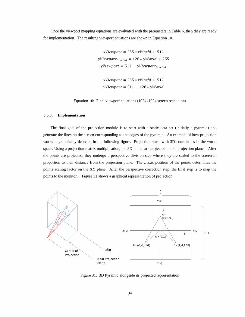
34
Once the viewport mapping equations are evaluated with the parameters in Table 6, then they are ready
for implementation. The resulting viewport equations are shown in Equation 10.
𝑥𝑉𝑖𝑒𝑤𝑝𝑜𝑟𝑡 = 255 ∗ 𝑥𝑊𝑜𝑟𝑙𝑑 + 512
𝑦𝑉𝑖𝑒𝑤𝑝𝑜𝑟𝑡𝑖𝑛𝑣𝑒𝑡𝑒𝑑 = 128 ∗ 𝑦𝑊𝑜𝑟𝑙𝑑 + 255
𝑦𝑉𝑖𝑒𝑤𝑝𝑜𝑟𝑡 = 511 − 𝑦𝑉𝑖𝑒𝑤𝑝𝑜𝑟𝑡𝑖𝑛𝑣𝑒𝑡𝑒𝑑
𝑥𝑉𝑖𝑒𝑤𝑝𝑜𝑟𝑡 = 255 ∗ 𝑥𝑊𝑜𝑟𝑙𝑑 + 512
𝑦𝑉𝑖𝑒𝑤𝑝𝑜𝑟𝑡 = 511 − 128 ∗ 𝑦𝑊𝑜𝑟𝑙𝑑
Equation 10: Final viewport equations (1024x1024 screen resolution)
3.5.3: Implementation
The final goal of the projection module is to start with a static data set (initially a pyramid) and
generate the lines on the screen corresponding to the edges of the pyramid. An example of how projection
works is graphically depicted in the following figure. Projection starts with 3D coordinates in the world
space. Using a projection matrix multiplication, the 3D points are projected onto a projection plane. After
the points are projected, they undergo a perspective division step where they are scaled to the screen in
proportion to their distance from the projection plane. The z axis position of the points determines the
points scaling factor on the XY plane. After the perspective correction step, the final step is to map the
points to the monitor. Figure 31 shows a graphical representation of projection.
Figure 31: 3D Pyramid alongside its projected representation
Near Projection Plane
zFarCenter of Projection
x
y
C = (1,-1,1.99)B = (-1,-1,1.99)
A = (1,0,1.99)
D = (0,0,1)
Y=2
Y=-2
X=2X=-24
4

35
When testing the initial module it was necessary to send in the four coordinates (xStart, yStart, xEnd,
yEnd) to the rasterizer in parallel. This meant creating 4 instances of the projection, perspective division
and viewport mapping blocks. This approach ensures that the signals arrived to the line drawer (rasterizer)
at the same time allowing the rasterizer to perform its rasterization. It became clear in implementation that
while this method worked in simulation, it did not synthesize for a larger design with a larger lookup table.
Additionally, because of the use of a combinational lookup table needed to synthesize such a design,
routing the design became a problem for the place and route stage of the implementation. Figure 32 shows
the initial integration.
Figure 32: Initial Integration of Coordinate Generator, Viewport Projector and Rasterizer
The solution to the problem was to reduce the four instances into only one instance, and the first step in
designing the projector and viewport module is to layout the block diagram and its inputs/outputs. The top
level module (Figure 33) is synchronous and contains a coordAxis, dataValid, coordValue, depthValue and
coordNumUnderProcess as inputs. The outputs are the window coordinates which are sent to the line
drawer (covered in the next section). The internal blocks of the projectorViewport module are shown in
Figure 34. Finally, Figure 35 and 36 show the simulation of the Fetcher/Projector module.
Figure 33: Projector / Viewport Mapper Block
Figure 34: Internal Blocks of the Coordinate Projector and Viewport Mapper
End Point Generator
State Machine Projection
Projection
Perspective Division
Perspective Division
Viewport Mapping
Viewport Mapping
Rasterization
{ x,y,z }
{ x,y,z }
{ xp,yp }
{ xp,yp }
{ xp / z,yp /z}
{ xp / z,yp /z}
{ xc,yc }
{ xc,yc }
rasterizerDone
clock coordAxis dataValid coordVal[1..-11] depthVal[1..-11]
windowCoordinate[9..0] windowStartX[9..0] windowStartY[9..0] windowEndX[9..0] windowEndY[9..0]
clock coordAxis dataValid
coordVal[1..-11] depthVal[1..-11]
windowCoordinate[9..0] windowStartX[9..0] windowStartY[9..0] windowEndX[9..0] windowEndY[9..0]
clock dataValid signDividend signDivisor dividend[0..-11] divisor[1..-11] coordNumUnderProcess[2..0]
result[1..-11]
clock coordAxis dataValid coordProjectedPerspective[1..-11]
windowCoordinate[9..0]
clock dataValid windowCoordinate[9..0] coordNumUnderProcess[2..0]
windowStartX[9..0] windowStartY[9..0] windowEndX[9..0] windowEndY[9..0]
0
clock
coordAxis
dataValid coordVal[1..-11] depthVal[1..-11]
windowCoordinate[9..0] coordNumUnderProcess[2..0]
windowStartX[9..0] windowStartY[9..0] windowEndX[9..0] windowEndY[9..0]
viewportTransformer:viewportTx coordinateRegister:coordReg lutDivider:perspectiveDivision
coordNumUnderProcess[2..0] coordNumUnderProcess[2..0]
projectorViewport:coordProjector

36
Figure 35: Behavioral Simulation of Fetcher/Projector with Several Line Vertices Generated
0111
1111
11
0111
1111
1101
1111
1111
0111
1111
11
000
000
000
000
433
427
454
427
451
497
498
513
498
454
433
451
454
498
497
513
498
511
511
511
511
0000
0000
0000
0
0000
0000
0000
000
0000
0000
000
0000
0000
0000
0
00
00
0
/ras
teriz
erTo
pTB_
v/g p
uTop
/pro
jVie
wpo
rt/c
oord
Pro j
ecto
r/co
ordR
eg/c
lock
/ ras
teriz
erTo
pTB_
v/gp
uTop
/pro
j Vie
wpo
rt/c
oord
Proj
ecto
r/co
ordR
e g/w
indo
wCo
ordi
nate
0111
1111
11
0111
1111
1101
1111
1111
0111
1111
11
/ras
teriz
erTo
pTB_
v/g p
uTop
/pro
j Vie
wpo
rt/c
oord
Proj
ecto
r/co
ordR
eg/c
oord
Num
Und
erPr
oces
s00
000
000
000
0
/ ras
teriz
erTo
pTB_
v/gp
uTop
/pro
jVie
wpo
rt/c
oord
Proj
ecto
r/co
ordR
eg/d
ataV
alid
/ ras
teriz
erTo
pTB_
v/gp
uTop
/pro
jVie
wpo
rt/c
oord
Proj
ecto
r/co
ordR
e g/w
indo
wSt
artX
433
427
454
427
451
/ ras
teriz
erTo
pTB_
v/gp
uTop
/pro
jVie
wpo
rt/c
oord
Proj
ecto
r/co
ordR
eg/w
indo
wSt
artY
497
498
513
498
/ras
teriz
erTo
pTB_
v/gp
uTop
/pro
j Vie
wpo
rt/c
oord
Proj
ecto
r/co
ordR
e g/w
indo
wEn
dX45
443
345
145
4
/ ras
teriz
erTo
pTB_
v/gp
uTop
/pro
jVie
wpo
rt/c
oord
Proj
ecto
r/co
ordR
e g/w
indo
wEn
dY49
849
751
349
8
/ras
teriz
erTo
pTB_
v/g p
uTop
/pro
j Vie
wpo
rt/c
oord
Proj
ecto
r/vi
ewpo
rtTx
/clo
ck
/ras
teriz
erTo
pTB_
v/gp
uTop
/pro
j Vie
wpo
rt/c
oord
Proj
ecto
r/vi
ewpo
rtTx
/coo
rdAx
is
/ras
teriz
erTo
pTB_
v/gp
uTop
/pro
jVie
wpo
rt/c
oord
Proj
ecto
r/vi
ewpo
rtTx
/dat
aVal
id
/ ras
teriz
erTo
pTB_
v/gp
uTop
/pro
jVie
wpo
rt/c
oord
Pro j
ecto
r/vi
ewpo
rtTx
/win
dow
Coor
dina
te51
151
151
151
1
/ ras
teriz
erTo
pTB_
v/gp
uTop
/pro
jVie
wpo
rt/c
oord
Proj
ecto
r/vi
ewpo
rtTx
/coo
rdPr
ojec
tedP
ersp
ectiv
e00
0000
0000
000
0000
0000
0000
000
0000
0000
000
0000
0000
0000
0
/ras
teriz
erTo
pTB_
v/gp
uTop
/pro
jVie
wpo
rt/c
oord
Pro j
ecto
r/vi
ewpo
rtTx
/coo
rdPr
ojec
tedP
ersp
ectiv
eFix
ed0
00
00
+25
1608
0000
0 ps
1612
0000
0 ps
1616
0000
0 ps
Entit
y:ra
ster
izer
TopT
B_v
Arch
itect
ure:
fast
Dat
e:W
edSe
p14
10:1
4:22
AMPa
cific
Day
light
Tim
e20
11Ro
w:
1Pa
ge:
1

37
Figure 36: Behavioral Simulation of Fetcher/Projector with a single line endpoint shown
0111
1111
1101
1010
101
110
0000
000
101
1100
011
001
1111
001
001
1111
1111
000
001
010
011
100
000
454
427
498
513
451
454
513
498
511
427
513
454
498
511
0000
0000
0000
010
0101
0100
010
1000
0000
0100
110
0011
1001
010
0000
0011
1010
000
0000
0000
000
0-0
.329
102
-0.0
0439
453
-0.2
2363
30.
0566
406
0
/ras
teriz
erTo
pTB_
v/g p
uTop
/pro
jVie
wpo
rt/c
oord
Pro j
ecto
r/co
ordR
eg/c
lock
/ras
teriz
erTo
pTB_
v/gp
uTop
/pro
j Vie
wpo
rt/c
oord
Proj
ecto
r/co
ordR
e g/w
indo
wCo
ordi
nate
0111
1111
1101
1010
101
110
0000
000
101
1100
011
001
1111
001
001
1111
1111
/ras
teriz
erTo
pTB_
v/g p
uTop
/pro
j Vie
wpo
rt/c
oord
Proj
ecto
r/co
ordR
eg/c
oord
Num
Und
erPr
oces
s00
000
101
001
110
000
0
/ ras
teriz
erTo
pTB_
v/gp
uTop
/pro
jVie
wpo
rt/c
oord
Proj
ecto
r/co
ordR
eg/d
ataV
alid
/ras
teriz
erTo
pTB_
v/gp
uTop
/pro
jVie
wpo
rt/c
oord
Proj
ecto
r/co
ordR
e g/w
indo
wSt
artX
454
427
/ ras
teriz
erTo
pTB_
v/gp
uTop
/pro
jVie
wpo
rt/c
oord
Proj
ecto
r/co
ordR
eg/w
indo
wSt
artY
498
513
/ras
teriz
erTo
pTB_
v/gp
uTop
/pro
j Vie
wpo
rt/c
oord
Proj
ecto
r/co
ordR
e g/w
indo
wEn
dX45
145
4
/ras
teriz
erTo
pTB_
v/gp
uTop
/pro
jVie
wpo
rt/c
oord
Proj
ecto
r/co
ordR
e g/w
indo
wEn
dY51
349
8
/ras
teriz
erTo
pTB_
v/g p
uTop
/pro
j Vie
wpo
rt/c
oord
Proj
ecto
r/vi
ewpo
rtTx
/clo
ck
/ras
teriz
erTo
pTB_
v/gp
uTop
/pro
j Vie
wpo
rt/c
oord
Proj
ecto
r/vi
ewpo
rtTx
/coo
rdAx
is
/ras
teriz
erTo
pTB_
v/gp
uTop
/pro
jVie
wpo
rt/c
oord
Pro j
ecto
r/vi
ewpo
rtTx
/dat
aVal
id
/ ras
teriz
erTo
pTB_
v/gp
uTop
/pro
jVie
wpo
rt/c
oord
Pro j
ecto
r/vi
ewpo
rtTx
/win
dow
Coor
dina
te51
142
751
345
449
851
1
/ras
teriz
erTo
pTB_
v/gp
uTop
/pro
jVie
wpo
rt/c
oord
Proj
ecto
r/vi
ewpo
rtTx
/coo
rdPr
ojec
tedP
ersp
ectiv
e00
0000
0000
000
1001
0101
0001
010
0000
0001
001
1000
1110
0101
000
0000
1110
100
0000
0000
0000
0
/ras
teriz
erTo
pTB_
v/gp
uTop
/pro
jVie
wpo
rt/c
oord
Pro j
ecto
r/vi
ewpo
rtTx
/coo
rdPr
ojec
tedP
ersp
ectiv
eFix
ed0
-0.3
2910
2-0
.004
3945
3-0
.223
633
0.05
6640
60
1613
2000
0 ps
1613
6000
0 ps
1614
0000
0 ps
Entit
y:ra
ster
izer
TopT
B_v
Arch
itect
ure:
fast
Dat
e:W
edSe
p14
10:1
8:11
AMPa
cific
Day
light
Tim
e20
11Ro
w:
1Pa
ge:
1

38
3.5.4: Design Challenges
The first challenge to overcome was determining how to quickly divide two fixed point numbers.
Before finding a suitable solution, the first method was to try to divide two numbers by using an unsigned
binary divider. Unfortunately, because both binary numbers were in fixed point representation, the division
operation produced incorrect results due to differences from fractional representation as compared to binary
whole numbers. The solution to this problem was to either use a fixed point algorithm or to use a division
method called multiplication by the reciprocal of the divisor which is shown schematically in Figure 37 and
38. This method seemed most feasible for the division operation that needed to be implemented. To test
this solution a binary lookup table was created which included all possible combinations of bits. Initially,
the weighted sum of each bit multiplied by its fractional representation was computed and then stored and
the closest matching value was used. After this method was used the more reliable method of using a base
10 fraction to base 2 fixed point converter (presented in the Appendix C) was used. The code was modified
to work with an array of numbers in base 10 fixed point precision format.
Figure 37: High Speed Division by Reciprocal Multiplication [23]
The next step was to construct the lookup table. The lookup table began with 2999 entries. A case
statement based LUT was created which was then converted to a block ram with initialized contents.
Figure 38: Perspective Divider (using Reciprocal Lookup Multiplication Method)
Reciprocal ROM Multiplier
z 1/z
x
x/z
WE DATAIN[13..0] WADDR[11..0] RADDR[11..0] DATAOUT[13..0]
SYNC_RAM
0
+ A[12..0] B[12..0]
ADDER
D EN A Q PR E
CL R D EN A
Q PR E CL R
D Q PR E
EN A CL R
= A[11..0] B[11..0]
EQUAL
x A[11..0] B[13..0]
MULTIPLIER D Q PR E EN A
CL R D Q PR E EN A
CL R
D EN A
Q PR E CL R
D EN A
Q PR E CL R
SEL DATAA DATAB OUT0
MUX21
SEL DATAA DATAB OUT 0
MUX21 mem
14' h0000 -- 12' h000 --
A dd0 1' h1 --
13' h17FD --
dataValidReg
dividendReg[0..-11]
Equal0 12' h400 --
reciprocalDivisor[-1..-14]
signProduct signProductReg
signDividend signDivisor
clock
dataValid
dividend[0..-11]
divisor[1..-11]
result[1..-11] coordNumUnderProcess[2..0] product~[13..0]
14' h2000 --
Mult0 product[25..14]
result~[12..0] 13' h0000 --
dataValidReg2 signProductReg~0
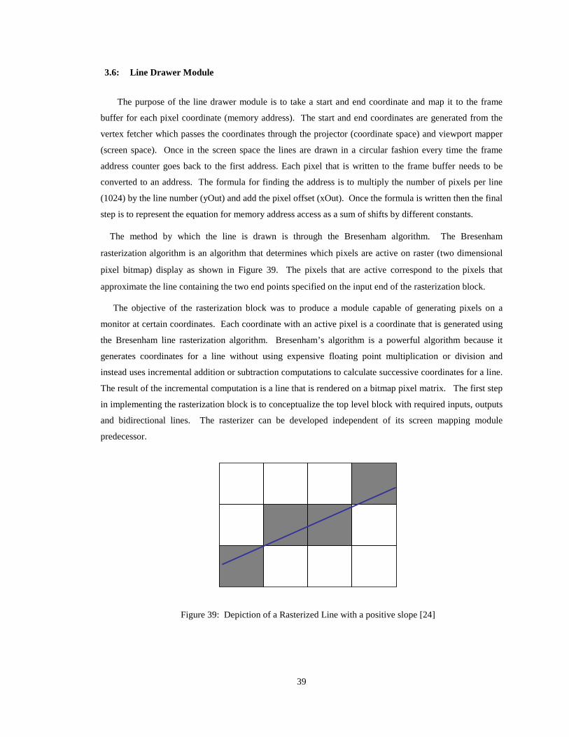
39
3.6: Line Drawer Module
The purpose of the line drawer module is to take a start and end coordinate and map it to the frame
buffer for each pixel coordinate (memory address). The start and end coordinates are generated from the
vertex fetcher which passes the coordinates through the projector (coordinate space) and viewport mapper
(screen space). Once in the screen space the lines are drawn in a circular fashion every time the frame
address counter goes back to the first address. Each pixel that is written to the frame buffer needs to be
converted to an address. The formula for finding the address is to multiply the number of pixels per line
(1024) by the line number (yOut) and add the pixel offset (xOut). Once the formula is written then the final
step is to represent the equation for memory address access as a sum of shifts by different constants.
The method by which the line is drawn is through the Bresenham algorithm. The Bresenham
rasterization algorithm is an algorithm that determines which pixels are active on raster (two dimensional
pixel bitmap) display as shown in Figure 39. The pixels that are active correspond to the pixels that
approximate the line containing the two end points specified on the input end of the rasterization block.
The objective of the rasterization block was to produce a module capable of generating pixels on a
monitor at certain coordinates. Each coordinate with an active pixel is a coordinate that is generated using
the Bresenham line rasterization algorithm. Bresenham’s algorithm is a powerful algorithm because it
generates coordinates for a line without using expensive floating point multiplication or division and
instead uses incremental addition or subtraction computations to calculate successive coordinates for a line.
The result of the incremental computation is a line that is rendered on a bitmap pixel matrix. The first step
in implementing the rasterization block is to conceptualize the top level block with required inputs, outputs
and bidirectional lines. The rasterizer can be developed independent of its screen mapping module
predecessor.
Figure 39: Depiction of a Rasterized Line with a positive slope [24]

40
3.6.1: State Machine
The state machine for the line generator consists of 6 states (idle, setup1, setup2, setup3, rasterization,
and done). Originally the state machine was written with two states for each pixel generation. The final
state machine consists of one state per pixel. Pseudo code for the state machine is depicted below (Figure
40).
public void lineBresenham(int x0, int y0, int x1, int y1, Color color) { int pix = color.getRGB(); int dy = y1 - y0; int dx = x1 - x0; int stepx, stepy; if (dy < 0) { dy = -dy; stepy = -1; } else { stepy = 1; } if (dx < 0) { dx = -dx; stepx = -1; } else { stepx = 1; } dy <<= 1; // dy is now 2*dy dx <<= 1; // dx is now 2*dx raster.setPixel(pix, x0, y0); if (dx > dy) { int fraction = dy - (dx >> 1); // same as 2*dy - dx while (x0 != x1) { if (fraction >= 0) { y0 += stepy; fraction -= dx; // same as fraction -= 2*dx } x0 += stepx; fraction += dy; // same as fraction -= 2*dy raster.setPixel(pix, x0, y0); } } else { int fraction = dx - (dy >> 1); while (y0 != y1) { if (fraction >= 0) { x0 += stepx; fraction -= dy; } y0 += stepy; fraction += dx; raster.setPixel(pix, x0, y0); } } }
Figure 40: Bresenham Rasterizer pseudo code [25]

41
After understanding the pseudocode, it was converted to a state machine in Verilog. The first step was
to convert the pseudocode to distinct states. The states are shown in Figure 41 and Table 7 below. A
description of the function of each state is provided alongside the states. As mentioned before the first step
was to receive the reset signal at which point the first setup state was reached. This setup state takes the
input coordinates and performs initial delta calculations on the coordinates. Additionally, it moves to
second setup state which finds the two delta values. Any sequential code presented in the previous page
that requires a computed result to be put into a secondary setup state. Finally, the third setup state then
calculates the actual next line. In the rasterization state, the line is incremented in accordance with the delta
calculations performed in the previous steps. When the coordinate counters reach the final coordinate (end)
value, the rasterization done signal is issued. The loop back arrows in the figure show the preservation of
the state variables. The only time the state is issued a state transition request is when the state calculations
and conditions are complete.
Figure 41: State Machine for Line Generator Block
State Name Description IDLE_STATE Waits for new line pulse to go to first setup state SETUP_STATE_1 Calculates delta values of input coordinates SETUP_STATE_2 Calculates 2xdelta values of input coordinates SETUP_STATE_3 Calculates slope based on delta values RASTERIZATION_STATE Calculates successive pixel coordinates until end RASTERIZATION_DONE Asserts finished signal and de-asserts writing signal
Table 7: Line Generator State Description
Cond: (~reset)
Cond: 1
Cond1: (!(deltaX>deltaY) && (yOut!=y1))Cond2: ((deltaX>deltaY) && (xOut!=x1))
Cond: 1
Cond: 1
Cond: 1
Cond: (newLine|startRasterization)
Cond: !(newLine|startRasterization)
Cond1: (!(deltaX>deltaY) && !(yOut!=y1))Cond2: ((deltaX>deltaY) && !(xOut!=x1)) IDLE_STATE
SETUP_STATE_1
SETUP_STATE_2
SETUP_STATE_3
RASTERIZATION_STATE
RASTERIZATION_DONE

42
The last step was to connect the line generator to the video generation module and verify that a line
could be drawn. The primary steps consist of generating X,Y pairs and sending them to the frame buffer
(dual port block ram) which is configured to work as a circular buffer. The final step is to stream to pixel
data and color data to the LCD monitor. The formula for finding the address in block ram for an input x,
and y coordinate is address = 1024y+x. This equation can be hardware optimized to simply perform a shift
by the log base 2 of the constant coefficient multiplier. The final optimized equation is a = yout <<10 + x.
This results in a savings of a multiplier (assuming there is no optimization during elaboration of the RTL
code). The block diagram is shown below (Figure 42).
Figure 42: Top Level Block Diagram of Line Generator
The first integration task was to connect a static line generator to the video generator and frame buffer
and observer the monitor draw a static line on the screen. The next step was to create a pattern of four lines
on the screen and alter the pattern based on the mouse position. The initial and final versions of the system
tasks are depicted Figure 43 and Figure 44.
Figure 43: Implementation tasks for the Static Line Generator
To DVI Tx
rasterizer_top.vLine Drawer
USER_CLK
FPGA_CPU_RESET_B
x0 {start}
y0 {start}
x1 {end}
y1 {end}
I2C_SCL_DVI
I2C_SDA_DVI
XCLK_P
XCLK_N
H_SYNC
V_SYNC
DATA_ENABLE
DATA
MO
USE
_CLK
MO
USE
_DAT
A
From Screen Mapper
To PS/2 Mouse Controller
GenerateCoordinates
Write Pixel Values
To Frame Buffer
Read Frame Buffer and
Stream Pixels to Monitor
Start Coord
End Coord

43
After creating the static line generator the final step was to create an animated line generator based on
the position of the mouse (displacement values) and to demonstrate that the lines moved in accordance with
the coordinate values.
Figure 44: Implementation tasks for the Dynamic Line Generator
The initial output results of the line generator are shown below (Figure 45). They consist of two
cursor positions (center and left). The left image depicts a centered cursor position while the right image
depicts a left aligned cursor position. As the cursor moves the four lines stretch and move to form the
appropriate shape.
Figure 45: Results from Cursor Position Based Line Generator
The rasterizer module takes in a start and end coordinate which is sent in by an internal state
machine and generates the lines corresponding to the start and end points. The state machine draws and un-
draws 4 lines when the mouse changes position. The rasterizer connects to the screen map module, the
DVI transmitter module and the PS/2 mouse module.
In summary, the Bresenham algorithm was converted from pseudo code to a Verilog state
machine. The state machine generates coordinates that send the color values of each coordinate to a
corresponding Block RAM frame buffer. The frame buffer is a 1024 X 1024 with a single bit depth of
color. A color depth of 1 corresponds to a monochrome image with only two colors. A behavioral
simulation of the single line (addresses) is presented in the following page (Figure 46). It starts from the
origin to the maximum address in the frame buffer (1024x1024).
Generate Coordinates
Clear Frame on Every Change
in Mouse Position
Read Frame Buffer and
Stream Pixels to Monitor
Start Coord
End Coord

44
Figure 46: Behavioral Simulation of Single Line Generator
0 0 1023
1023
0000
1111
x0
1025
2050
3075
4100
5125
6150
7175
8200
9225
1025
011
275
/pix
elW
riter
TB/c
loc k
/ pix
elW
riter
TB/r
eset
/pix
elW
riter
TB/x
00
/ pix
elW
riter
TB/y
00
/pix
elW
riter
TB/x
110
23
/pix
elW
riter
TB/y
110
23
/pix
elW
riter
TB/a
ctio
n
/pix
elW
riter
TB/n
ewLi
ne
/ pix
elW
riter
TB/c
olor
Dep
th00
0011
11
/pix
elW
riter
TB/f
inis
hed
/pix
elW
riter
TB/b
rese
nham
Writ
ing
/ pix
elW
riter
TB/b
rese
nham
Setu
p
/pix
elW
riter
TB/a
ddre
ssx
010
2520
5030
7541
0051
2561
5071
7582
0092
2510
250
1127
5
/glb
l/GS R
1000
00 p
s12
0000
ps
1400
00 p
s16
0000
ps
1800
00 p
s20
0000
ps
2200
00 p
s24
0000
ps
Entit
y:pi
xelW
riter
TBAr
chite
ctur
e:fa
stD
ate:
Wed
Sep
217:
06:0
2PM
Paci
ficD
aylig
htTi
me
2011
Row
:1
Page
:1

45
3.7: Frame Buffer
The purpose of the frame buffer is to accept color and coordinate values and input them into a block of
memory for one frame of video. From there the pixel reader circularly reads the pixels and output them to
the monitor. The frame buffer stores 1024x1024 (~1 Million) monochrome (color depth of 1) pixels.
Dual port ram is used to display the contents of the graphical object as pixels. Additionally, dual port RAM
can read and write at the same time and is used for bridging two clock regions. For purposes of this
project, the frame buffer is used to display single pixels per address but can be configured to display higher
pixel color depths for specific applications. A suitable SRAM controller was located from OpenCores.org
(developed by Victor Lopez Lorenzo) before the decision was made to use exclusively on-chip memory.
The SRAM and DPRAM are shown in Figure 47. The on-chip memory contains space for approximately 5
megabits of data whereas the off chip SRAM contains approximately 9.4 megabits of data supporting a
higher resolution of pixels. The need to shift from SRAM to BRAM was due to the fact that the SRAM
controller did not properly send data to the FPGA at the 100MHz speed requested. Eventually, the SRAM
controller was abandoned and a dual port block RAM method was used to communicate video frames to
the monitor and store the frames. Because DPRAM is directly embedded in the FPGA, it can be run at
much faster speeds than the SRAM. More importantly, because SRAM is not on the FPGA and has no
ability to allow for simultaneous reads or writes, the SRAM is less suitable for using for a frame buffer that
requires concurrent reads and writes. This limitation resulted in use of the DPRAM on the FPGA.
Figure 47: SRAM Interface versus DPRAM Module The frame buffer was finally converted into 64 smaller sized frame buffer modules which allowed for
clearing contents in parallel (64 times the original clear rate) as compared to a single frame buffer
instantiation. The final frame buffer, comprised of an input encoder (one hot shifter logic), the sixty-four
32Kbit block rams and the output multiplexer are presented in Figure 48.
address_in(17:0)
burst_type_extension(1:0)
cycle_type_identifier(2:0)
data_in(35:0)
select_input(3:0)
clk
cycle
read_request
reset
strobe
write_enable
write_request
data_out(35:0)
SRAM_FLASH_ADDR(17:0)
acknowledge
data_out_valid
error
SRAM_ADV_LD_B
SRAM_BW0
SRAM_BW1
SRAM_BW2
SRAM_BW3
SRAM_CLK
SRAM_CS_B
SRAM_FLASH_WE_B
SRAM_MODE
SRAM_OE_B
SRAM_FLASH_DATA_PAR(35:0)
RAM
CLKA
RSTA
ENA
WEA
xx
CLKB
RSTB
ENB
WEB
1048576 11048576 1
ADDRA(19:0)
DIA(0:0)
DIB(L:R)
ADDRB(19:0)
DOB(0:0)
DOA(L:R)write_enable
write_clock
write_address(19:0)
write_data
read_enable
read_clock
read_address(19:0)
read_data
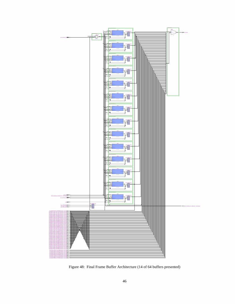
46
Figure 48: Final Frame Buffer Architecture (14 of 64 buffers presented)
multiplexer:readDataMux
bin2OneHotEncoder:readEncoder
frameBuffer:FRAME_BUFFER[63].frameBuf
frameBuffer:FRAME_BUFFER[62].frameBuf
frameBuffer:FRAME_BUFFER[61].frameBuf
frameBuffer:FRAME_BUFFER[60].frameBuf
frameBuffer:FRAME_BUFFER[59].frameBuf
frameBuffer:FRAME_BUFFER[58].frameBuf
frameBuffer:FRAME_BUFFER[57].frameBuf
frameBuffer:FRAME_BUFFER[56].frameBuf
frameBuffer:FRAME_BUFFER[55].frameBuf
frameBuffer:FRAME_BUFFER[54].frameBuf
frameBuffer:FRAME_BUFFER[53].frameBuf
frameBuffer:FRAME_BUFFER[52].frameBuf
frameBuffer:FRAME_BUFFER[51].frameBuf
frameBuffer:FRAME_BUFFER[50].frameBuf
D
E NA
Q
P RE
CL R
DA TA IN[0 ]
WE
CL K 0
WA DDR[1 3 ..0 ]
RA DDR[1 3 ..0 ]
DA TA O UT[0 ]
S Y NC_ RA M
D
E NA
Q
P RE
CL R
DA TA IN[0 ]
WE
CL K 0
WA DDR[1 3 ..0 ]
RA DDR[1 3 ..0 ]
DA TA O UT[0 ]
S Y NC_ RA M
D
E NA
QP RE
CL R
DA TA IN[0 ]
WE
CL K 0
WA DDR[1 3 ..0 ]
RA DDR[1 3 ..0 ]
DA TA O UT[0 ]
S Y NC_ RA M
D
E NA
QP RE
CL R
DA TA IN[0 ]
WE
CL K 0
WA DDR[1 3 ..0 ]
RA DDR[1 3 ..0 ]
DA TA O UT[0 ]
S Y NC_ RA M
D
E NA
QP RE
CL R
DA TA IN[0 ]
WE
CL K 0
WA DDR[1 3 ..0 ]
RA DDR[1 3 ..0 ]
DA TA O UT[0 ]
S Y NC_ RA M
D
E NA
QP RE
CL R
DA TA IN[0 ]
WE
CL K 0
WA DDR[1 3 ..0 ]
RA DDR[1 3 ..0 ]
DA TA O UT[0 ]
S Y NC_ RA M
D
E NA
QP RE
CL R
DA TA IN[0 ]
WE
CL K 0
WA DDR[1 3 ..0 ]
RA DDR[1 3 ..0 ]
DA TA O UT[0 ]
S Y NC_ RA M
D
E NA
QP RE
CL R
DA TA IN[0 ]
WE
CL K 0
WA DDR[1 3 ..0 ]
RA DDR[1 3 ..0 ]
DA TA O UT[0 ]
S Y NC_ RA M
D
E NA
Q
P RE
CL R
DA TA IN[0 ]
WE
CL K 0
WA DDR[1 3 ..0 ]
RA DDR[1 3 ..0 ]
DA TA O UT[0 ]
S Y NC_ RA M
D
E NA
QP RE
CL R
DA TA IN[0 ]
WE
CL K 0
WA DDR[1 3 ..0 ]
RA DDR[1 3 ..0 ]
DA TA O UT[0 ]
S Y NC_ RA M
D
E NA
QP RE
CL R
DA TA IN[0 ]
WE
CL K 0
WA DDR[1 3 ..0 ]
RA DDR[1 3 ..0 ]
DA TA O UT[0 ]
S Y NC_ RA M
D
E NA
QP RE
CL R
DA TA IN[0 ]
WE
CL K 0
WA DDR[1 3 ..0 ]
RA DDR[1 3 ..0 ]
DA TA O UT[0 ]
S Y NC_ RA M
D
E NA
QP RE
CL R
DA TA IN[0 ]
WE
CL K 0
WA DDR[1 3 ..0 ]
RA DDR[1 3 ..0 ]
DA TA O UT[0 ]
S Y NC_ RA M
D
E NA
QP RE
CL R
DA TA IN[0 ]
WE
CL K 0
WA DDR[1 3 ..0 ]
RA DDR[1 3 ..0 ]
DA TA O UT[0 ]
S Y NC_ RA M
D
E NA
Q
P RE
CL R
<<A[63..0]
COUNT[5..0]
L E FT_ S HIFT
S E L [5 ..0 ]
DA TA [6 3 ..0 ]O UT
MUX
mem_DATAOUT[0]read_clock_OUT0
read_enable_OUT0
bin2OneHotEncoder:writeEncoder_oneHotOutput
bin2OneHotEncoder:readEncoder_oneHotOutput
frameBuffer:FRAME_BUFFER[48].frameBuf_read_dataframeBuffer:FRAME_BUFFER[47].frameBuf_read_dataframeBuffer:FRAME_BUFFER[46].frameBuf_read_dataframeBuffer:FRAME_BUFFER[45].frameBuf_read_dataframeBuffer:FRAME_BUFFER[44].frameBuf_read_dataframeBuffer:FRAME_BUFFER[43].frameBuf_read_dataframeBuffer:FRAME_BUFFER[42].frameBuf_read_dataframeBuffer:FRAME_BUFFER[41].frameBuf_read_dataframeBuffer:FRAME_BUFFER[40].frameBuf_read_dataframeBuffer:FRAME_BUFFER[39].frameBuf_read_dataframeBuffer:FRAME_BUFFER[38].frameBuf_read_dataframeBuffer:FRAME_BUFFER[37].frameBuf_read_dataframeBuffer:FRAME_BUFFER[36].frameBuf_read_dataframeBuffer:FRAME_BUFFER[35].frameBuf_read_dataframeBuffer:FRAME_BUFFER[34].frameBuf_read_dataframeBuffer:FRAME_BUFFER[33].frameBuf_read_dataframeBuffer:FRAME_BUFFER[32].frameBuf_read_dataframeBuffer:FRAME_BUFFER[31].frameBuf_read_dataframeBuffer:FRAME_BUFFER[30].frameBuf_read_dataframeBuffer:FRAME_BUFFER[29].frameBuf_read_dataframeBuffer:FRAME_BUFFER[28].frameBuf_read_dataframeBuffer:FRAME_BUFFER[27].frameBuf_read_dataframeBuffer:FRAME_BUFFER[26].frameBuf_read_dataframeBuffer:FRAME_BUFFER[25].frameBuf_read_dataframeBuffer:FRAME_BUFFER[24].frameBuf_read_dataframeBuffer:FRAME_BUFFER[23].frameBuf_read_dataframeBuffer:FRAME_BUFFER[22].frameBuf_read_dataframeBuffer:FRAME_BUFFER[21].frameBuf_read_dataframeBuffer:FRAME_BUFFER[20].frameBuf_read_dataframeBuffer:FRAME_BUFFER[19].frameBuf_read_dataframeBuffer:FRAME_BUFFER[18].frameBuf_read_dataframeBuffer:FRAME_BUFFER[17].frameBuf_read_dataframeBuffer:FRAME_BUFFER[16].frameBuf_read_dataframeBuffer:FRAME_BUFFER[15].frameBuf_read_dataframeBuffer:FRAME_BUFFER[14].frameBuf_read_dataframeBuffer:FRAME_BUFFER[13].frameBuf_read_dataframeBuffer:FRAME_BUFFER[12].frameBuf_read_dataframeBuffer:FRAME_BUFFER[11].frameBuf_read_dataframeBuffer:FRAME_BUFFER[10].frameBuf_read_data
frameBuffer:FRAME_BUFFER[9].frameBuf_read_data
frameBuffer:FRAME_BUFFER[8].frameBuf_read_dataframeBuffer:FRAME_BUFFER[7].frameBuf_read_dataframeBuffer:FRAME_BUFFER[6].frameBuf_read_dataframeBuffer:FRAME_BUFFER[5].frameBuf_read_dataframeBuffer:FRAME_BUFFER[4].frameBuf_read_dataframeBuffer:FRAME_BUFFER[3].frameBuf_read_dataframeBuffer:FRAME_BUFFER[2].frameBuf_read_dataframeBuffer:FRAME_BUFFER[1].frameBuf_read_dataframeBuffer:FRAME_BUFFER[0].frameBuf_read_data
read_data[0]~reg0
clock
write_address[19..0]
write_data
read_address[19..0]
mem
read_data[0]~reg0
mem
read_data[0]~reg0
mem
read_data[0]~reg0
mem
read_data[0]~reg0
mem
read_data[0]~reg0
mem
read_data[0]~reg0
read_data[0]~reg0
mem
read_data[0]~reg0
mem
read_data[0]~reg0
mem
read_data[0]~reg0
mem
read_data[0]~reg0
read_data[0]~reg0
mem
read_data[0]~reg0
read_data[0]~reg0read_data
Mux0
ShiftLeft0
6 4 ' h 0 0 0 0 0 0 0 0 0 0 0 0 0 0 0 1 - -
mem
mem
mem

47
3.8: Video Generator
The final stage in the pipeline design is the video generator and pixel multiplexer. It takes in RGB data
values across three 8-bit channels and converts them into a 12-bit multiplexed data which combine to
produce a 24-bit RGB data. Since the models use single bit color and the fact that the design is running at
1024x1024, this means that the module needs to extend the color bits. Each 12-bit burst of data consists of
the RGB data repeated (if less than 8 bits per color channel) to fill with the 8-bit channel. The chip
responsible for the transmission of video synchronization and data signals is the Chrontel 7301C
transmitter. The transmitter can be configured to run in DVI or VGA bypass modes, in which the output
data is configured to output in a single analog port for each color channel. When configured for DVI mode,
the transmitter sends a data stream that directly compatible for a digital monitor.
The slave (CH7301C) at address 0x76 (on an I2C line) is initialized from the FPGA using I2C bus
master. I2C is a two wire serial protocol similar to the mouse protocol in that it contains two signals (clock
and data). When the master is ready to transmit data to the slave, it does so by initializing the address of
transfer. The I2C slave responds with “acknowledge” if the address transferred matches the address value
of the slave device. Onc acknowledge is passed to the master on the data line, then the master starts
transmitting 8-bit data values after it indicated the write status to the slave. Figure 49 shows the I2C
timing diagram.
Figure 49: I2C Protocol [26]
Once the FPGA initializes the DVI transmitter for the appropriate mode (DVI or analog bypass), the
DVI transmitter begins streaming video data to the monitor. The primary signals needed for a DVI
transmission are the pixel clock, horizontal sync, vertical sync, data, data enable. The video controller
parameters and I2C initialization were modified from existing video parameters that were part of two
separate existing modules which were combined to produce initial test patterns on the monitor. Video
timing parameters for the video generator were created from the XFree86 modeline generator [27].
Video Parameter Horizontal Pixels Vertical Lines Active Width 1024 1024 Front Porch 32 20 Synch Width 376 11 Back Porch 32 21 Total 1432 1076
Table 8: Video Parameters
SC L SD A S A7 A6 A5 A4 A3 A2 A1 R W ack D7 D6 D5 D4 D3 D2 D1 D 0 nack P

48
The timing diagram below (Figure 50) shows the monitor signals generated by the CH7301C. The
vertical synchronization pulse is not shown because it does not fit within the confined view. The vertical
synchronization pulse needs 1024 lines which go beyond the figure width. A summary of the parameters
used for the video generator is shown below the figure. The columns in the table depict the parameters,
the horizontal and vertical parameters.
Figure 50: Video Timing Diagram
The next step in the design was to construct the primary logic for the video module. The video module
(Figure 51) outputs red green and blue signals based the counter values presented by the synchronization
generator. The video color signals are finally multiplexed (12 bits at a time) to the digital monitor.
Figure 51: Video Generator
D QPRE
ENA
CLR
D QPRE
ENA
CLR
<CIN
A[10..0]
B[10..0]
LESS_THAN
<CIN
A[10..0]
B[10..0]
LESS_THAN
<CIN
A[10..0]
B[10..0]
LESS_THAN
<CIN
A[10..0]
B[10..0]
LESS_THAN
D QPRE
ENA
CLR
SELDATAA
DATABOUT0
MUX21
1
1
1
1
pixelClk
data_enable
hCount[10..0]
vCount[10..0]
red_out[7..0]
green_out[7..0]
LessThan0
11' h000 --
LessThan1
11' h3FF --
data_enable~0
red_out[7..0]~reg0
concat~[3..0]
4' h0 --
data_enable~1
blue_out[7..0]~reg0
dataRGB_in[3..0]
LessThan2
11' h000 --
data_enable~2LessThan3
11' h3FF --
blue_out[7..0]
green_out[7..0]~reg0
Pixel Clock
Horizontal Sync
Data Stream
Data Enable
Active Video - 1024 Pixels
Horizontal Sync Width 1432 Pixels
Back Porch 32 Pixels Front Porch 32 Pixels
Pulse Width 344 Pixels

49
Figure 52: Pixel Multiplexer (Input to Chrontel 7301C)
D
ENA
QPRE
CLR
D
ENA
QPRE
CLR
D
ENA
QPRE
CLR
D
ENA
QPRE
CLR
D
ENA
QPRE
CLR
D
ENA
QPRE
CLR
D
ENA
QPRE
CLR
D
ENA
QPRE
CLR
D
ENA
QPRE
CLR
D
ENA
QPRE
CLR
D
ENA
QPRE
CLR
D
ENA
QPRE
CLR
<CIN
A[10..0]
B[10..0]
LESS_THAN
1
<CIN
A[10..0]
B[10..0]
LESS_THAN
1
<CIN
A[10..0]
B[10..0]
LESS_THAN
1
<CIN
A[10..0]
B[10..0]
LESS_THAN
1
D
ENA
QPRE
CLR
010
010
SEL
DATAA
DATABOUT0
MUX21
SELDATAADATAB
OUT0
MUX21
SELDATAADATAB
OUT0
MUX21
always0~0
always0~1always0~2
data[0]~reg0
data[2]~reg0
data[4]~reg0
data[5]~reg0
data[6]~reg0
data[7]~reg0
data[8]~reg0
data[9]~reg0
data[10]~reg0
data[11]~reg0LessThan0
11' h000 --
LessThan1
11' h3FF --
LessThan2
11' h000 --
LessThan3
11' h3FF --
pixel_select
pixel_select~0pixel_select~1
data~[11..0]
data~[23..12]
12' h000 --
data~[35..24]
12' h000 --
clock
reset
data_enable (GND)
hCount[10..0]
vCount[10..0]
red[7..0]green[7..0]
blue[7..0]
data[11..0]
data[3]~reg0
data[1]~reg0

50
Chapter 4: Results
This section presents the frame buffer results after applying rotation transformation to the object. The
primary means of extracting the frame buffer contents for a stationary non-moving object was to export the
contents of the memory array from Modelsim. The contents of the frame buffer are displayed on the
monitor. First the orthographic projection result is shown on Figure 53 which does not rely upon the
reciprocal ROM to compute the projected coordinates. Figure 54 shows the results of projection of the
object which undergoes perspective distortion and therefore shows points closer together which have a
higher depth coordinate.
Figure 53: Orthographic (parallel) projected teapot
Figure 54: Perspective (convergent) projected teapot
GPU Parameter Numerical Value Maximum (Adjustable) NUM_VERTICES_IN_OBJECT 480 512 NUM_QUADS_IN_OBJECT 448 512
Table 9: Summary of Object Parameters

51
Rotation about Y Axis (0 Degrees) Rotation about X Axis (0 Degrees)
Rotation about Y Axis (30 Degrees) Rotation about X Axis (30 Degrees)
Rotation about Y Axis (60 Degrees) Rotation about X Axis (60 Degrees)
Rotation about Y Axis (90 Degrees) Rotation about X Axis (90 Degrees)
Table 10: Application of rotation transformation with various angles

52
After applying the rotation of the four different angles across two axes, the next step was to check how
the rotation across two axes displayed on the frame buffer. Two rotation angles were used (30 and 60
degrees) and they were applied across x and y axes. The final results are shown in Table 11.
30 Degree Rotation (x then y) 60 Degree Rotation (x then y)
Table 11: Rotation across both x and y

53
Chapter 5: Conclusion
The project was a success because the primary goals of learning the graphics pipeline and designing the
system were achieved. There were difficulties encountered during the project. The first difficulty was that
there was a considerable learning curve to overcome since this was the first time developing on an FPGA.
Additionally, familiarizing with the 3D pipeline was challenging in the beginning. To overcome this
challenge, an incremental approach was taken to familiarize with the pipeline. The mouse module was the
first module that was created, which was followed by the video generator. Outputting to the on board
LEDs proved to uncover several cases where the state machine was remaining in the same state. There
were modules in the design that were not used in the end and one of them was the SRAM frame buffer
interface. As covered before, the SRAM frame buffer was not able to output back values to the graphics
video generator. A decision was made to abandon the SRAM module and instead use the Dual Port RAMS
on the FPGA. Finally, the projection module started off by drawing random lines. After several iterations it
was discovered that the timing was the main issue for this. To resolve timing, delay registers were placed
to allow for the signals to line up. Additionally, the perspective divider needed to be corrected to produce
the proper product (quotient).

54
Chapter 6: Future Work
There are several areas that can be explored to further enhance the project. A primary enhancement is
to continue automating the generation of the binary fixed point values. When using the original fixed point
binary generation script there was a need to export the binary data manually and combine the results. The
binary conversion script is shown in Appendix C. There was an initial development on automating the
acquisition and generation of the binary fixed point values from the input dataset. Unfortunately, XST
(Xilinx Synthesis Tool) does not support real data types in synthesis even if the intent is to use the real data
types for only elaboration and file generation. To overcome this limitation, a temporary solution was found
which was to take the data and run it in behavioral simulation. The non-synthesizable instructions not
supported by XST were commented out of the code and $readmemb system task was used to read in the
data generated by behavioral elaboration. Tcl (Tool Command Language) could have been used to
enhance the automation of this fixed point generation problem but, due to time constraints, this method was
not explored in the project.
The next development applicable to the project is to employ a shader which requires an exponentiation
look-up table and a pixel color interpolator. A first development can be to design a flat (single color)
shading and then to change it to a smooth shader. The mouse trackball can be used to rotate the light
source to change the position of the light aiming on the object. Finally, clipping is needed to prevent the
rasterizer from drawing unnecessary lines that are not part of the object. This can be done using either
scissoring (image space clipping) directly on the frame buffer or clipping (object space vertex removal)
which is done prior to the object being displayed on the screen.
The design is currently a static pipeline. It could be converted to a programmable pipeline which can
run alongside an embedded processor (Microblaze) using C instructions. This hardware/software co-
design option was explored but not implemented because it did not add any measurable difference to the
desired results.

55
References
[1] Angel, Edward. “Interactive computer graphics: a top-down approach with OpenGL”. 3rd ed. Toronto: Addison Wesley, 2003.
[2] Teo, Leonard. "CG Science for Artists Part 2: The Real-Time Rendering Pipeline | CG Channel."
CG Channel - News, Videos, Training and Community for Entertainment Artists. [Accessed February 5, 2011.] http://www.cgchannel.com/2010/11/cg-science-for-artists-part-2-the-real-time-rendering-pipeline/
[3] "Xilinx University Program XUPV5-LX110T Development Platform." FPGA, CPLD, and EPP
Solutions from Xilinx, Inc. November 15, 2010. [Accessed September 25, 2011.] http://www.xilinx.com/products/boards-and-kits/XUPV5-LX110T.htm
[4] Virtex 4 FX12 Evaluation Kit Product Brief.,
[Accessed September 25, 2011.] http://www.em.avnet.com/ctf_shared/evk/df2df2usa/Xilinx_Virtex-4_FX12_Evaluation_Kit_- _Product_Brief.pdf [5] Digilent Inc. - Digital Design Engineer's Source. Digilent Inc., [Accessed September 25, 2011.] http://www.digilentinc.com/Products/Detail.cfm?NavPath=2,400,794&Prod=XUPV2P [6] Spartan 3E Starter Kit Image., http://members.optusnet.com.au/jekent/Images/Spartan-3E-Starter-Kit.gif
[Accessed September 25, 2011.]
[7] ML507 Image., [Accessed September 25, 2011.] http://www.xilinx.com/products/devkits/HW-V5-ML507-UNI-G-image.htm [8] Virtex 5 Family Overview. [Accessed September 25, 2011.] http://www.xilinx.com/support/documentation/data_sheets/ds100.pdf [9] Virtex 4 Family Overview [Accessed September 25, 2011.] http://www.xilinx.com/support/documentation/data_sheets/ds112.pdf [10] Spartan 3 FPGA Family Data Sheet [Accessed September 25, 2011.]
http://www.xilinx.com/support/documentation/data_sheets/ds312.pdf [11] Virtex 2 Pro Product Information [Accessed September 25, 2011.]
http://www.digilentinc.com/Products/Detail.cfm?Prod=XUPV2P [12] Pong, Chu. FPGA prototyping by Verilog examples Xilinx Spartan -3 version. Hoboken, Wiley & Sons, 2008. [13] Microchip PS/2 to USB Mouse Translator Datasheet http://ww1.microchip.com/downloads/en/AppNotes/91055C.pdf [14] Chapweske, Adam. "The PS/2 Mouse/Keyboard Protocol." Computer-Engineering.org. [Accessed September 25, 2011.] http://www.computer-engineering.org/ps2protocol/ [15] 2D Transforms lecture notes. Ohio State University [Accessed September 11, 2011] http://www.cse.ohio-state.edu/~parent/classes/581/Lectures/5.2DtransformsAhandout.pdf]

56
[16] 2D Rotation Notes [Accessed September 25, 2011.] http://www.siggraph.org/education/materials/HyperGraph/modeling/mod_tran/2drota.htm [17] 3D Rotation Notes [Accessed September 25, 2011.] http://www.siggraph.org/education/materials/HyperGraph/modeling/mod_tran/3drota.htm [18] Hudachek-Buswell, Mary R., Addition and Subtraction with Signed-Magnitude Data (Mano, Section 10-2)., Basics Seminar, CSc 8215 High Performance Computing (2005 Fall) [Accessed September 25, 2011.] http://web.cecs.pdx.edu/~mperkows/CLASS_573/573_2007/Addition%20and%20Subtraction%20 with%20Signed-Magnitude%20Data%20(Mano.ppt [19] Kator, Andrew., Legaz, Jennifer., Quick Tips in Art & Design: Depth [Accessed September 12, 2011.] http://articles.katorlegaz.com/quicktipsinartanddesign/depth/0802one-point.jpg [20] From World to Screen Lecture Notes [Accessed September 12, 2011.] http://www-users.aston.ac.uk/~cornford/cs2150/pdf/window2vp_lec_8up.pdf [21] Chapter 4: Word Windows Viewports & Clipping
[Accessed September 29, 2011.] http://www.di.ubi.pt/~agomes/cg/teoricas/04e-windows.pdf [22] World Windows, Viewports & Clipping Slides [Retrieved June 9, 2011.] http://www.di.ubi.pt/~agomes/cg/teoricas/04e-windows.pdf [23] Petrov, Boko Baev., “Time Optimized Fixed Point Algorithm for Unsigned Division Operation in
Programmable Logic Devices” September 2004 [Retrieved June 19, 2011.] http://ecad.tu-sofia.bg/et/2004/Papers/Microelectronics/Paper-B_Petrov.pdf
[24] “Computer Graphics – Scan Line Conversion,” [Retrieved September 24, 2011.] http://cs.gettysburg.edu/~skim/cs373/lectures/02_ScanLineConversion_Line.pdf [25] Line Drawing [Accessed February 12, 2011.]
http://wwwx.cs.unc.edu/~mcmillan/comp136/Lecture6/Lines.html [26] Herveille, Richard., “I2C-Master Core Specification” [Retrieved September 24, 2011.] ftp://ftp.gwdg.de/pub/misc2/opencores/cores/i2c/i2c_rev03.pdf [27] XFree86 Modeline Generator [Retrieved January 20, 2011.]
http://xtiming.sourceforge.net/cgi-bin/xtiming.pl

57
Appendix A: GPU Source Code
datasetReader.vh /********************************************************************** * Module Name: datasetReader * File Name: datasetReader.vh * * Author: Vahe Robert Jabagchourian * California, State University Northridge * * Creation Date: October 9, 2011 * * Description: Contains the dataset (OFF) specific * format parser. * Note: this will only run and generate the * file during behavioral elaboration. **********************************************************************/ `include "../headers/parameters.vh" `include "../headers/fixedPoint.vh" `include "../headers/rotation.vh" `ifndef datasetReader_vh `define datasetReader_vh module datasetReader; parameter ADDR = 9; parameter EOF = 32'hffff_ffff; parameter NULL = 0; parameter MAX_LINE_CHARS = 100; parameter IN_FILE = "teapot.off"; parameter MEM_FILE = "teapot.mem"; parameter X_AXIS = 3'b100; parameter Y_AXIS = 3'b010; parameter Z_AXIS = 3'b001; integer lineIndexParsed = 0; fixedPoint fixedPointLibrary(); rotation rotationLibrary(); //##################################################################### //Begin memory initialization block //##################################################################### //File reader modified from - http://chris.spear.net/pli/fileio.htm task initializeLUT; integer numVertices; //Defined in OFF (object file format) dataset integer numTriangles; //Defined in OFF (object file format) dataset integer numPrimitiveVertices; //3 for triangle, 4 for quad, etc... integer numLines; //File variables integer inputFile; //file handle integer outputFile; //file handle integer scaledFile; integer line; //line handle

58
real xCoordinate, yCoordinate, zCoordinate; real xCoordinateScaled, yCoordinateScaled, zCoordinateScaled; real angleOfRotation; real xCoordinateRotated_xAxis, yCoordinateRotated_xAxis, zCoordinateRotated_xAxis; real xCoordinateRotated_yAxis, yCoordinateRotated_yAxis, zCoordinateRotated_yAxis; real scalingFactor; integer vertexIndex1, vertexIndex2, vertexIndex3; begin //Open input OFF file for reading inputFile = $fopen(IN_FILE, "r"); //Open output MEM file for writing outputFile = $fopen(MEM_FILE, "w"); scaledFile = $fopen("scaled.off", "w"); //Check for existence of file if (inputFile == NULL) begin $display ("Input file %s not found!", inputFile); end //Line Number Line Content //Line 1: [NUM_VERTICES] [NUM_TRIANGLES] [NUM_LINES] //Line 2: [X_COORDINATE] [Y_COORDINATE] [Z_COORDINATE] // ... //Line 2+NUM_VERTICES: [X_COORDINATE] [Y_COORDINATE] [Z_COORDINATE] //Line 2+NUM_VERTICES+1: //[TRIANGLE_LINE_INDEX_1][TRIANGLE_LINE_INDEX_2][TRIANGLE_LINE_INDEX_3] //Line 2+NUM_VERTICES+1+NUM_TRIANGLES: //[TRIANGLE_LINE_INDEX_1][TRIANGLE_LINE_INDEX_2][TRIAGNLE_LINE_INDEX_3] //Read first line values
line = $fscanf(inputFile, "%d %d %d", numVertices, numTriangles, numLines);
lineIndexParsed = lineIndexParsed + 1; //$display("%d", numVertices); while (line != -1) //while (!$feof(infile)) begin if (lineIndexParsed <= numVertices) begin
//Use fscanf to read the formatted data from //filestream as opposed to sscanf to read data from //string
line = $fscanf(inputFile, "%f %f %f", xCoordinate, yCoordinate, zCoordinate);
scalingFactor = 1.5;//2.45; xCoordinateScaled = xCoordinate*scalingFactor; yCoordinateScaled = yCoordinate*scalingFactor; zCoordinateScaled = ((zCoordinate-
2.5)*scalingFactor)+2.5;
//Rotate using an index of 85 of 1024 which //corresponds to 30 degrees on the specified axis

59
//(index of 1024 is 30 degrees) angleOfRotation = rotationLibrary.indexToAngle(10'd1023 - 10'd255); rotationLibrary.rotate(xCoordinateScaled, yCoordinateScaled, zCoordinateScaled, X_AXIS, angleOfRotation, xCoordinateRotated_xAxis, yCoordinateRotated_xAxis, zCoordinateRotated_xAxis);
//Rotate using an index of 85 of 1024 which
//corresponds to 30 degrees on the specified axis //(index of 1024 is 30 degrees)
angleOfRotation = rotationLibrary.indexToAngle(10'd170); rotationLibrary.rotate(xCoordinateRotated_xAxis, yCoordinateRotated_xAxis, zCoordinateRotated_xAxis, X_AXIS, angleOfRotation, xCoordinateRotated_xAxis, yCoordinateRotated_xAxis, zCoordinateRotated_xAxis);
angleOfRotation = rotationLibrary.indexToAngle(10'd170);
rotationLibrary.rotate(xCoordinateRotated_xAxis, yCoordinateRotated_xAxis, zCoordinateRotated_xAxis, Y_AXIS, angleOfRotation, xCoordinateRotated_yAxis, yCoordinateRotated_yAxis, zCoordinateRotated_yAxis);
//$fwrite(scaledFile, "%f\t%f\t%f\n", xCoordinateRotated_xAxis, yCoordinateRotated_xAxis, zCoordinateRotated_xAxis);
$fwrite(outputFile, "%42b", {fixedPointLibrary.binaryFraction(xCoordinateRotated_yAxis),fixedPointLibrary.binaryFraction(yCoordinateRotated_yAxis),fixedPointLibrary.binaryFraction(zCoordinateRotated_yAxis)});
$fwrite(outputFile, "\n"); $display("%f %f %f\n", xCoordinate, yCoordinate, zCoordinate);
//$display("%b %f\n", fixedPointLibrary.binaryFraction(zCoordinate), zCoordinate);
//$display("%d\n", lineIndexParsed); end else if (lineIndexParsed > numVertices) begin
line = $fscanf(inputFile, "%d %d %d %d", numPrimitiveVertices, vertexIndex1, vertexIndex2, vertexIndex3);
//$display("%d %d %d %d", numPrimitiveVertices, //vertexIndex1, vertexIndex2, vertexIndex3);
60
end //Go to next line index lineIndexParsed = lineIndexParsed + 1; end //initialize rest of memory content to 0
for (lineIndexParsed = numVertices+1; lineIndexParsed <= (2**ADDR); lineIndexParsed = lineIndexParsed+1)
begin if (lineIndexParsed == 2**ADDR) begin $fwrite(outputFile, "%b", {42{1'b0}}); end
else if (lineIndexParsed < 2**ADDR) begin $fwrite(outputFile, "%b\n", {42{1'b0}}); end end $fclose(outputFile); $fclose(inputFile); $fclose(scaledFile); $display ("Vertex Memory Content Loaded!");
end endtask
endmodule `endif

61
fixedPoint.vh /********************************************************************** * Module Name: fixedPoint * File Name: fixedPoint.vh * * Author: Vahe Robert Jabagchourian * California, State University Northridge * * Creation Date: October 9, 2011 * * Description: Contains the fixed point and rotation * functions necessary to automate the * fixedPoint conversion process. **********************************************************************/ `ifndef fixedPoint_vh `define fixedPoint_vh module fixedPoint; parameter COORDINATE_MSB = 2; parameter COORDINATE_LSB = -11; //Returns integer component of the fractional decimal in base 10 function integer truncate; input real fractionalDecimal; begin truncate = $rtoi(fractionalDecimal); end endfunction function integer greatestExponentBase2LessThan; input integer decimalInteger; integer binaryExponent; begin binaryExponent = 0; //Check the next value to see if it as a power of two is
//less than or equal to binaryInteger while (2**(binaryExponent+1) <= decimalInteger) begin binaryExponent = binaryExponent + 1; end greatestExponentBase2LessThan = binaryExponent; end endfunction function [COORDINATE_MSB:0] decimalToBinary; input integer decimalInteger; integer decimalValueRemainder; //Result of subtraction of
//decimalInteger from greatestPowerOf2LessThan integer greatestExponentOfBase2LessThanDecimalValue; begin decimalToBinary = {COORDINATE_MSB{1'b0}}; //Initialize decimalValueRemainder = decimalInteger;

62
//Iteratively subtract the greatest power of two less than //the decimal integer until the result of subtraction is //equal to 0
while (decimalValueRemainder > 0) begin
greatestExponentOfBase2LessThanDecimalValue = greatestExponentBase2LessThan(decimalValueRemainder); decimalValueRemainder = decimalValueRemainder - 2**greatestExponentOfBase2LessThanDecimalValue;
decimalToBinary[greatestExponentOfBase2LessThanDecimalValue-1] = 1; end end endfunction //convert fractional signed magnitude number to binary function [COORDINATE_MSB:COORDINATE_LSB] binaryFraction; input real fractionalNumber; real currentFractionalNumber; real fractionalComponent; integer binaryFractionIndex; reg [COORDINATE_MSB:COORDINATE_LSB] binaryFractionVar; integer integerComponent; integer integerComponentIndex; begin fractionalComponent = 0; binaryFractionIndex = -1;
//Start index at the postition behind the decimal currentFractionalNumber = fractionalNumber;
//Initialize the currentFractionalNumber binaryFractionVar = {(COORDINATE_MSB
COORDINATE_LSB+1){1'b0}};
binaryFractionVar[COORDINATE_MSB] = currentFractionalNumber < 0;
//Convert only the magnitude of the unsigned integer
integerComponent = (currentFractionalNumber >= 0)? truncate(currentFractionalNumber) : truncate((-currentFractionalNumber));
binaryFractionVar[COORDINATE_MSB-1:0] = integerComponent; //Compute Fractional Component if (currentFractionalNumber < 0) begin
//Get the fractional part and handle negative numbers //by negating them to positive values fractionalComponent = -currentFractionalNumber - truncate(-currentFractionalNumber);
end else if (currentFractionalNumber > 0) begin
fractionalComponent = currentFractionalNumber - truncate(currentFractionalNumber);
end

63
else if (currentFractionalNumber == 0) begin fractionalComponent = 0; end //Perform the conversion //Keep multiplying the fraction by 2 and make sure that the //fractional component is non-zero
while (fractionalComponent != 0 && binaryFractionIndex >= COORDINATE_LSB)
begin fractionalComponent = fractionalComponent * 2; //If the magnitude of 2 * fractionalComponent is
//greater than 2 //Then assign a 1 to the binaryFraction vector at the //binaryFraction index position binaryFractionVar[binaryFractionIndex] = (fractionalComponent >= 1)? 1'b1 : 1'b0;
//Update values binaryFractionIndex = binaryFractionIndex - 1;
currentFractionalNumber = fractionalComponent - truncate(fractionalComponent);
fractionalComponent = currentFractionalNumber; end binaryFraction = binaryFractionVar; end endfunction endmodule `endif

64
rotation.vh /********************************************************************** * Module Name: rotation.vh * File Name: rotation.vh * * Author: Vahe Robert Jabagchourian * California, State University Northridge * * Creation Date: October 9, 2011 * * Description: Contains the rotation function required * to generate a trigonometric ROM address * from an index value. **********************************************************************/ module rotation; parameter X_AXIS = 3'b100; parameter Y_AXIS = 3'b010; parameter Z_AXIS = 3'b001; parameter UNSIGNED = 0; parameter SIGNED = 1; real deltaAngle = 0.00613592315154256; //Verilog Sin/Cosine Transcendental Functions //http://www.cse.lehigh.edu/~caar/marnold/
// papers/sanjose_hdlcon.doc function real sin; input x; real x; real x1,y,y2,y3,y5,y7,sum,sign; begin sign = 1.0; x1 = x; if (x1<0) begin x1 = -x1; sign = -1.0; end while (x1 > 3.14159265/2.0) begin x1 = x1 - 3.14159265; sign = -1.0*sign; end y = x1*2/3.14159265; y2 = y*y; y3 = y*y2; y5 = y3*y2; y7 = y5*y2; sum = 1.570794*y - 0.645962*y3 + 0.079692*y5 - 0.004681712*y7; sin = sign*sum; end endfunction

65
function real cos; input x; real x; begin cos = sin(x + 3.14159265/2.0); end endfunction //Rotator Task task rotate;
//(xCoord, yCoord, zCoord, axisRot, theta, // xCoordinateRotated, yCoordinateRotated, zCoordinateRotated)
input real xCoordReal; input real yCoordReal; input real zCoordReal; input reg [2:0] rotationAxis; input real rotationAngle; output real xCoordinateRotated; output real yCoordinateRotated; output real zCoordinateRotated; begin case (rotationAxis) //Rotation about x //x'=x //y'=y(cosθ) - z(sinθ) //z'=y(sinθ) + z(cosθ) X_AXIS: begin //Hold X //Transform Y and Z //x'=x xCoordinateRotated = xCoordReal; //y'=y(cosθ) - z(sinθ)
yCoordinateRotated = (yCoordReal * cos(rotationAngle)) – ((zCoordReal - 2.5) * sin(rotationAngle)); //z'=y(sinθ) + z(cosθ)
zCoordinateRotated = (yCoordReal * sin(rotationAngle)) + ((zCoordReal - 2.5) * cos(rotationAngle)) + 2.5;
end //Rotation about y //x'=x(cosθ) - z(sinθ) //y'=y //z'=z(cosθ) - x(sinθ) Y_AXIS: begin //x'=x(cosθ) - z(sinθ) xCoordinateRotated = (xCoordReal *
cos(rotationAngle)) + ((zCoordReal - 2.5) * sin(rotationAngle));
//y'=y yCoordinateRotated = yCoordReal; //z'=y(sinθ) + z(cosθ)

66
zCoordinateRotated = -(yCoordReal * sin(rotationAngle)) + ((zCoordReal - 2.5) * cos(rotationAngle)) + 2.5;
end Z_AXIS: begin //Rotation about z //x'=x*cosθ-ysinθ xCoordinateRotated = (xCoordReal *
cos(rotationAngle)) - (yCoordReal * sin(rotationAngle)); //y'=x*sinθ+ycosθ
yCoordinateRotated = (xCoordReal * sin(rotationAngle)) + (yCoordReal * cos(rotationAngle));
//z'=z zCoordinateRotated = zCoordReal; end endcase end endtask real angle; function real indexToAngle; input [10:0] index; begin indexToAngle = deltaAngle * index; end endfunction real realCoordinate; //11 bits fraction function real fixedToReal; input [2:-11] coordinate; begin fixedToReal = (-1**coordinate[2]) * ( coordinate[1] * 2 + coordinate[0] * 1 + coordinate[-1] * 0.5 + coordinate[-2] * 0.25 + coordinate[-3] * 0.125 + coordinate[-4] * 0.0625 + coordinate[-5] * 0.03125 + coordinate[-6] * 0.015625 + coordinate[-7] * 0.0078125 + coordinate[-8] * 0.00390625 + coordinate[-9] * 0.001953125 + coordinate[-10] * 0.0009765625 + coordinate[-11] * 0.0004882815 ); end endfunction endmodule

67
rotationUnit.v `timescale 1ns / 1ps /********************************************************************** * Module Name: rotationUnit * File Name: rotationUnit.v * * Author: Vahe Robert Jabagchourian * California, State University Northridge * * Creation Date: July 26, 2011 * * Description: Completes the rotation equation sum or * difference for one coordinate * x, y, or z. * In order to rotate first subtract 2.5 * (center of viewing frustum) from object * then perform the actual rotation * operation then add 2.5 to the rotated * object to place back in original center. * Table of Subtraction/Addition of Sign * Magnitude Binary Values * http://web.cecs.pdx.edu/~mperkows/ * CLASS_573/573_2007/ * Addition%20and%20Subtraction%20with * %20Signed- * Magnitude%20Data%20(Mano.ppt * * * Revisions: * July 26, 2011 Initial Module Created * August 22, 2011 Added conditional "add by 2.5" statements * in the actual rotation operation * calculation * Additionally, added parameters to * indicate that the rotationUnit is * altering the Z * October 7, 2011 Moved add subtract units to respective * functions **********************************************************************/ module rotationUnit(clock, reset, operation, coordinateProduct1, coordinateProduct2, coordinateRotated, axisOfRotation); /*********************************************************************** PARAMETERS **********************************************************************/ parameter COORDINATE_MSB = 2; //Sign Bit parameter COORDINATE_LSB = -11; //Last Fractional Bit parameter FALSE = 0;

68
parameter TRUE = 1; parameter ADD = 0; parameter SUBTRACT = 1; parameter THIS_UNIT_ALTERS_Z = FALSE; parameter X_AXIS = 3'b100; parameter Y_AXIS = 3'b010; parameter Z_AXIS = 3'b001; input wire clock; input wire reset; input wire operation; input wire [COORDINATE_MSB:COORDINATE_LSB] coordinateProduct1; input wire [COORDINATE_MSB:COORDINATE_LSB] coordinateProduct2; input wire [2:0] axisOfRotation; output reg [COORDINATE_MSB:COORDINATE_LSB] coordinateRotated; /*********************************************************************** Function: Perform Rotation - in other words call the add subtract * units for to complete the rotation ****************************************************************/ function [COORDINATE_MSB:COORDINATE_LSB] rotate; input [COORDINATE_MSB:COORDINATE_LSB] inputA; input [COORDINATE_MSB:COORDINATE_LSB] inputB; input operation; begin
case (operation) ADD:
//add a and b, each operand is signed rotate = add(inputA, inputB); SUBTRACT:
//subtract a and b, each operand is signed rotate = subtract(inputA, inputB); endcase end endfunction function sign; input [COORDINATE_MSB:COORDINATE_LSB] operand; begin sign = operand[COORDINATE_MSB]; end endfunction function [1:-11] mag; input [COORDINATE_MSB:COORDINATE_LSB] operand; begin mag = operand[1:-11];

69
end endfunction function [1:-11] doAdd; input [1:-11] operandA; input [1:-11] operandB; begin doAdd = operandA + operandB; end endfunction function [1:-11] doSub; input [1:-11] operandA; input [1:-11] operandB; begin doSub = operandA - operandB; end endfunction function [COORDINATE_MSB:COORDINATE_LSB] addMagnitudes_posA; input [COORDINATE_MSB:COORDINATE_LSB] inputA; input [COORDINATE_MSB:COORDINATE_LSB] inputB; begin
if (THIS_UNIT_ALTERS_Z == TRUE && (axisOfRotation == X_AXIS || axisOfRotation == Y_AXIS))
begin //add = +(A+B)+2.5 addMagnitudes_posA = {1'b0, doAdd(mag(inputA),
mag(inputB))} + 14'b01010000000000; end else begin addMagnitudes_posA = {1'b0, doAdd(mag(inputA),
mag(inputB))}; end end endfunction function [COORDINATE_MSB:COORDINATE_LSB] addMagnitudes_negA; input [COORDINATE_MSB:COORDINATE_LSB] inputA; input [COORDINATE_MSB:COORDINATE_LSB] inputB; begin if (THIS_UNIT_ALTERS_Z == TRUE && (axisOfRotation == X_AXIS ||
axisOfRotation == Y_AXIS)) begin //add = -(A+B)+2.5 addMagnitudes_negA = 14'b01010000000000 –
{1'b0, doAdd(mag(inputA), mag(inputB))}; end else begin
addMagnitudes_negA = {1'b1, doAdd(mag(inputA), mag(inputB))};
end

70
end endfunction function [COORDINATE_MSB:COORDINATE_LSB] subtractMagnitudes_posA; input [COORDINATE_MSB:COORDINATE_LSB] inputA; input [COORDINATE_MSB:COORDINATE_LSB] inputB; begin if (mag(inputA) > mag(inputB)) begin if (THIS_UNIT_ALTERS_Z == TRUE && (axisOfRotation == X_AXIS
|| axisOfRotation == Y_AXIS)) begin //add = +(A-B)+2.5
subtractMagnitudes_posA = ({1'b0, doSub(mag(inputA), mag(inputB))} + 14'b01010000000000);
end else begin
subtractMagnitudes_posA = {1'b0, doSub(mag(inputA), mag(inputB))};
end end else if (mag(inputA) < mag(inputB)) begin if (THIS_UNIT_ALTERS_Z == TRUE && (axisOfRotation == X_AXIS
|| axisOfRotation == Y_AXIS)) begin //add = -(B-A)+2.5 = 2.5-(B-A) subtractMagnitudes_posA = 14'b01010000000000 –
{1'b0, doSub(mag(inputB), mag(inputA))};
end else begin subtractMagnitudes_posA = {1'b1, doSub(mag(inputB),
mag(inputA))}; end end else if (mag(inputA) == mag(inputB)) begin
if (THIS_UNIT_ALTERS_Z == TRUE && (axisOfRotation == X_AXIS || axisOfRotation == Y_AXIS))
begin //add = +(A-B)+2.5
subtractMagnitudes_posA = {1'b0, doSub(mag(inputA), mag(inputB))} + 14'b01010000000000;
end else begin subtractMagnitudes_posA = {1'b0,
doSub(mag(inputA), mag(inputB))}; end end end endfunction
71
function [COORDINATE_MSB:COORDINATE_LSB] subtractMagnitudes_negA; input [COORDINATE_MSB:COORDINATE_LSB] inputA; input [COORDINATE_MSB:COORDINATE_LSB] inputB; begin if (mag(inputA) > mag(inputB)) begin if (THIS_UNIT_ALTERS_Z == TRUE && (axisOfRotation ==
X_AXIS || axisOfRotation == Y_AXIS)) begin
//add = -(A-B)+2.5 = 2.5-(A-B) subtractMagnitudes_negA = 14'b01010000000000 –
{1'b0, doSub(mag(inputA), mag(inputB))}; end else begin
subtractMagnitudes_negA = {1'b1, doSub(mag(inputA), mag(inputB))};
end end else if (mag(inputA) < mag(inputB)) begin if (THIS_UNIT_ALTERS_Z == TRUE && (axisOfRotation ==
X_AXIS || axisOfRotation == Y_AXIS)) begin //add = +(B-A)+2.5
subtractMagnitudes_negA = {1'b0, doSub(mag(inputB), mag(inputA))} + 14'b01010000000000;
end else begin
subtractMagnitudes_negA = {1'b0, doSub(mag(inputB), mag(inputA))};
end end else if (mag(inputA) == mag(inputB)) begin
if (THIS_UNIT_ALTERS_Z == TRUE && (axisOfRotation == X_AXIS || axisOfRotation == Y_AXIS))
begin //add = +(A-B)+2.5
subtractMagnitudes_negA = {1'b0, doSub(mag(inputA), mag(inputB))} + 14'b01010000000000;
end else begin subtractMagnitudes_negA = {1'b0,
doSub(mag(inputA), mag(inputB))}; end end end endfunction

72
/**************************************************************** * Function: Perform Rotation - do an add on the fixed point * operands and do an appropriate shift
****************************************************************/ function [COORDINATE_MSB:COORDINATE_LSB] add; input [COORDINATE_MSB:COORDINATE_LSB] inputA; input [COORDINATE_MSB:COORDINATE_LSB] inputB; begin //If the signs of the both multiplied operands of the add
//operation are equal if (sign(inputA) == sign(inputB)) begin if (sign(inputA) == 0) begin add = addMagnitudes_posA(inputA, inputB); end else if (sign(inputA) == 1) begin add = addMagnitudes_negA(inputA, inputB); end end else if (sign(inputA) != sign(inputB)) begin if (sign(inputA) == 0) begin add = subtractMagnitudes_posA(inputA, inputB); end else if (sign(inputA) == 1) begin add = subtractMagnitudes_negA(inputA, inputB); end end end endfunction function [COORDINATE_MSB:COORDINATE_LSB] subtract; input [COORDINATE_MSB:COORDINATE_LSB] inputA; input [COORDINATE_MSB:COORDINATE_LSB] inputB; begin
//If the signs of the both multiplied operands of the add //operation are equal
if (sign(inputA) == sign(inputB)) begin if (sign(inputA) == 0) begin
subtract = subtractMagnitudes_posA(inputA, inputB);
end else if (sign(inputA) == 1) begin
subtract = subtractMagnitudes_negA(inputA, inputB);
end end else if (sign(inputA) != sign(inputB)) begin

73
if (sign(inputA) == 0) begin subtract = addMagnitudes_posA(inputA, inputB); end else if (sign(inputA) == 1) begin subtract = addMagnitudes_negA(inputA, inputB); end end end endfunction always @(posedge clock) begin if (!reset) begin coordinateRotated <= 0; end else begin
//basically, add or subtract the two coordinate //product numbers in fixed point format coordinateRotated <= rotate(coordinateProduct1, coordinateProduct2, operation);
end end endmodule

74
Appendix B: Modelsim Virtual Signal Commands
vsim> virtual signal {((sim:/sinCosROM_TB_v/cosine[1])? (-1.0):(1.0))* (((sim:/sinCosROM_TB_v/sine[0])? (1.0) : (0.0))+
((sim:/sinCosROM_TB_v/sine[-1])? (0.5) : (0.0))+ ((sim:/sinCosROM_TB_v/sine[-2])? (0.25) : (0.0))+ ((sim:/sinCosROM_TB_v/sine[-3])? (0.125) : (0.0))+ ((sim:/sinCosROM_TB_v/sine[-4])? (0.0625) : (0.0))+ ((sim:/sinCosROM_TB_v/sine[-5])? (0.03125) : (0.0))+ ((sim:/sinCosROM_TB_v/sine[-6])? (0.015625) : (0.0))+ ((sim:/sinCosROM_TB_v/sine[-7])? (0.0078125) : (0.0))+ ((sim:/sinCosROM_TB_v/sine[-8])? (0.00390625) : (0.0))+ ((sim:/sinCosROM_TB_v/sine[-9])? (0.001953125) : (0.0))+ ((sim:/sinCosROM_TB_v/sine[-10])? (0.0009765625) : (0.0))+ ((sim:/sinCosROM_TB_v/sine[-11])? (0.0004882815) : (0.0))+ ((sim:/sinCosROM_TB_v/sine[-12])? (0.000244140625): (0.0))+ ((sim:/sinCosROM_TB_v/sine[-13])? (0.000122070125) : (0.0))+ ((sim:/sinCosROM_TB_v/sine[-14])? (0.00006103515625) : (0.0)))} sineFixed vsim> add wave /sineCosine_ROM_TB_v/sineFixed vsim> virtual signal {((sim:/sinCosROM_TB_v/cosine[1])? (-1.0):(1.0))*
(((sim:/sinCosROM_TB_v/cosine[0])? (1.0) : (0.0))+ ((sim:/sinCosROM_TB_v/cosine[-1])? (0.5) : (0.0))+ ((sim:/sinCosROM_TB_v/cosine[-2])? (0.25) : (0.0))+ ((sim:/sinCosROM_TB_v/cosine[-3])? (0.125) : (0.0))+ ((sim:/sinCosROM_TB_v/cosine[-4])? (0.0625) : (0.0))+ ((sim:/sinCosROM_TB_v/cosine[-5])? (0.03125) : (0.0))+ ((sim:/sinCosROM_TB_v/cosine[-6])? (0.015625) : (0.0))+ ((sim:/sinCosROM_TB_v/cosine[-7])? (0.0078125) : (0.0))+ ((sim:/sinCosROM_TB_v/cosine[-8])? (0.00390625) : (0.0))+ ((sim:/sinCosROM_TB_v/cosine[-9])? (0.001953125) : (0.0))+ ((sim:/sinCosROM_TB_v/cosine[-10])? (0.0009765625) : (0.0))+ ((sim:/sinCosROM_TB_v/cosine[-11])? (0.0004882815) : (0.0))+ ((sim:/sinCosROM_TB_v/cosine[-12])? (0.000244140625): (0.0))+ ((sim:/sinCosROM_TB_v/cosine[-13])? (0.000122070125) : (0.0))+ ((sim:/sinCosROM_TB_v/cosine[-14])? (0.00006103515625) : (0.0)))} cosineFixed vsim> add wave /sineCosine_ROM_TB_v/cosineFixed
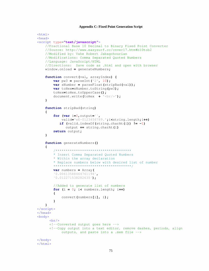
75
Appendix C: Fixed Point Generation Script
<html> <head> <script type="text/javascript"> //Fractional Base 10 Decimal to Binary Fixed Point Converter //Source: http://www.easysurf.cc/cnver17.htm#b10tob2 //Modified by: Vahe Robert Jabagchourian //Modifications: Comma Separated Quoted Numbers //Language: JavaScript/HTML //Directions: Save code as .html and open with browser window.onload = generateNumbers; function convert(val, arrayIndex) { var pw3 = parseInt("2", 10); var sNumber = parseFloat(stripBad(val)); var toHex=sNumber.toString(pw3); toHex=toHex.toUpperCase(); document.write(toHex + "<br/>"); } function stripBad(string) { for (var i=0,output='',
valid="eE-0123456789.";i<string.length;i++) if (valid.indexOf(string.charAt(i)) != -1) output += string.charAt(i) return output; } function generateNumbers() { /************************************* * Insert Comma Separated Quoted Numbers * Within the array declaration * Replace numbers below with desired list of number **************************************/ var numbers = Array( '0.00613588464761194', '0.012271538282635'); //Added to generate list of numbers for (i = 0; i< numbers.length; i++) { convert(numbers[i], i); } } </script> </head> <body> <br/> <!--Converted output goes here --> <!--Copy output into a text editor, remove dashes, periods, align outputs, and paste into a .mem file --> </body> </html>