processes

Article

Near-Wall Flow Characteristics of a CentrifugalImpeller with Low Specific Speed

Weidong Cao 1,2,* , Zhixiang Jia 1,2 and Qiqi Zhang 1,2

1 Research Institute of Fluid Engineering Equipment Technology, Jiangsu University, Zhenjiang 212013, China2 China National Research Center of Pumps, Jiangsu University, Zhenjiang 212013, China* Correspondence: cwd@ujs.edu.cn; Tel.: +86 1395-281-6468

Received: 14 July 2019; Accepted: 1 August 2019; Published: 5 August 2019�����������������

Abstract: In order to study the near-wall region flow characteristics in a low-specific-speed centrifugalimpeller, based on ANSYS-CFX 15.0 software, Reynolds averaged Navier-Stokes (RANS) methodsand renormalization group (RNG) k-ε turbulence model were used to simulate the whole flow fieldof a low specific speed centrifugal pump with five blades under different flow rates. Simulationresults of external characteristics of the pump were in good agreement with experimental results.Profiles were set on the pressure side and suction side of impeller blades at the distances of 0.5 mmand 2 mm, respectively, to study the distributions of flow characteristics near the wall region of fivegroups of blades. The results show that the near-wall region flow characteristics of five groups ofblades were similar, but the static pressure, relative velocity, cross flow velocity, and turbulent kineticenergy of profiles on the pressure side were quite different to those on the suction sides, and thesecharacteristics also changed with the alternation of flow rate. As the flow rate was 13 m3/h or 20 m3/h,within the radius range of 40 to 50 mm, there was an extent of negative relative velocity of the profileson the pressure side, and a counter-current happened not on the suction side, but on the pressure sidein the low specific speed centrifugal impeller. The flow characteristics of profiles at the distances of0.5 mm and 2 mm also showed a small difference.

Keywords: low specific speed; centrifugal pump; impeller; near-wall region; flow characteristics

1. Introduction

Low-specific-speed centrifugal pumps have the characteristics of small flow rate, large head,and low efficiency, which are widely used in aerospace, military industry, electric power, waterconservancy, chemical industry, and other important fields. After decades of efforts, with thecontinuous improvement of experimental means and the development of numerical calculationmethods for the internal flow of turbo-machinery, more understanding and consensus have beengained on the internal flow characteristics and more achievements have been achieved in hydraulicdesign optimization methods. Micro internal flow structure controlling has been the method forimproving the efficiency of centrifugal pumps with low specific speed.

Karrasik, a well-known pump expert in the United States, pointed out that since flow loss dependson the boundary layer, the efficiency of low-specific-speed centrifugal pumps can be improved byproperly controlling the boundary layer of the flow channel [1]. Young-Do et al. studied the internalflow and performance of a centrifugal pump impeller with very low specific speed through an externalcharacteristic test and particle image velocimetry (PIV) internal flow field test. The results show thatthere is a large recirculation at the outlet of a semi-open impeller, which significantly reduces theabsolute tangential velocity and thus reduces the pump’s head [2]. Westra et al. simulated the internalflow field of a low-specific-speed centrifugal pump, where Spalart and Allmaras’ turbulence modelwas selected and the near-wall mesh scale was dense, and found that the maximum error of the relative

Processes 2019, 7, 514; doi:10.3390/pr7080514 www.mdpi.com/journal/processes

Processes 2019, 7, 514 2 of 13

velocity obtained by PIV was 6%. From the relative velocity distribution, it can be seen that, fromthe pressure side of the blade to the suction side, when the velocity gradually increases to a certainmaximum, the relative velocity on the suction surface of the blade decelerates, and the jet-wake areadecreases with the increasing of flow rate. With the spatial change of the flow separation point, thesecondary flow structure and intensity also change continuously [3]. Pedersen et al. used PIV andlaser Doppler vibrometer to measure the flow inside the impeller of a centrifugal pump. It was foundthat there were two channels in the impeller under the condition of a small flow rate: the flow inone channel was controlled by the impeller rotation, which was similar to that under the design flowrate, while in the other channel, there was a relatively static stall and the entrance area of the bladewas blocked by a cluster, with edthe remaining part of the flow passage being occupied by somevortices [4]. Shao et al. used PIV technology to measure the velocity of the internal flow field of acentrifugal pump impeller with large blade outlet angle, there exists a low energy fluid wake regionwith relatively low velocity near the suction side of the blade, where there exists a jet region withrelatively high velocity while near the pressure side. The flow structure is especially obvious undersmall flow rates. These flow structures are the result of the interaction between the fluid viscosity,boundary layer, and secondary flow [5]. Tsujita and co-workers’ numerical simulation and experimentsshow that, if the boundary layer thickness of the suction side is larger than that of pressure side atthe inflection of the streamline in the impeller inlet area of the centrifugal pump, it will be helpfulto restrain the formation of vortices in the internal channel to reduce hydraulic loss [6]. Cui et al.’snumerical simulation of ultra-high speed and low specific speed centrifugal pumps with long andshort blades shows that the reflux zone mainly concentrates on the inlet of the long blade on the suctionside, the middle of the long blade on the pressure side, and the outlet of the short blade on the suctionside; these refluxes have a great influence on the internal and external characteristics of pumps [7].Limbach et al. simulated the cavitation flow of a low-specific-speed centrifugal pump under differentflow rates and different surface roughness conditions, and for non-cavitating flow, the measured andcalculated head are in good agreement. According to the measurement, for rough walls, net positivesuction head rises slightly higher [8]. Cao et al. studied the influence of the impeller eccentricity on theperformance of a low-specific-speed centrifugal pump, and found that with the impeller eccentricityincreasing, the head and efficiency become lower and the area of low pressure at the suction side of theshort blade inlet becomes gradually smaller; however, the area of low pressure at the suction side ofthe long blade inlet becomes larger, and the pressure at the impeller inlet and tongue become largertoo [9]. Zhang et al. simulated the start–stop process of three kinds of fluids in a low specific speedcentrifugal pump, and the effects of viscosity on transient performance, head-flow curve and internalflow structure in impeller and volute were studied. Results show that, the liquid with higher viscositythan water may reduce the operation reliability of low specific speed centrifugal pump during start-upperiod [10]. Chen et al. explored internal flow and its unsteady characteristics in a low-specific-speedcentrifugal pump. There were vortices in various sizes and numbers in flow channels of the impellerunder different flow conditions. A high velocity zone was found in two adjacent channels near thetongue. However, the zone disappeared gradually with the increase of flow rate [11]. Dong et. al.studied the effect of the front streamline wrapping angles variation of a low-specific-speed centrifugalimpeller on energy performance, the pressure pulsation, interior and exterior noise characteristics,where the front sweep angle variation was found to have an insignificant influence on centrifugalpump performance characteristics; however, it influences fluid hydrodynamics around the volutetongue [12]. The flow field in a low specific speed impeller was reconstructed by Zhang et. al. [13], theroot-mean-square error for pressure prediction was 0.84% and the velocity prediction error was within0.5 m/s, its computation time for the flow field prediction was less than 1/240 of the computational fluiddynamics. Proper orthogonal decomposition (POD) base modal analysis was carried out on the sampleset, and the base modal characteristic of the flow field and its energy distribution were analyzed.

The optimization design of low specific speed pumps and the study of large-scale flowcharacteristics have been carried out, but there are few studies on the flow characteristics near

Processes 2019, 7, 514 3 of 13

the blade wall. For this paper, ANSYS CFX 15.0 software used to simulate the unsteady flow of a lowspecific speed pump by analyzing the near-wall region flow on blades near the tongue and far from thetongue such that the distribution of viscous stress, relative velocity, and static pressure was obtained.

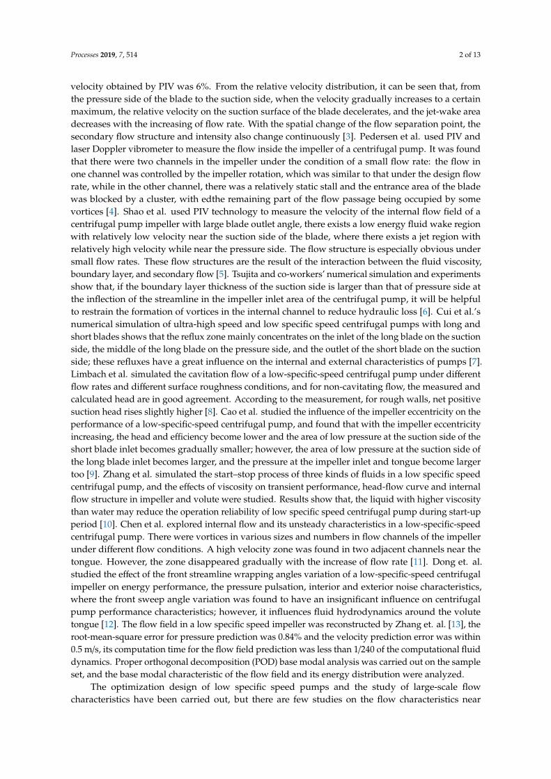
2. Geometric Model and Computational Grid

A low specific speed pump was designed with the following parameters: flow rate Q = 13 m3/h,head H = 26 m, rotational speed n = 2880 r/min, impeller inlet diameter D1 = 44 mm, outlet diameterD2 = 146 mm, outlet width b2 = 6 mm, blade outlet angle β2 = 40◦, blade wrap angle φ = 120◦, bladethickness from inlet to outlet was 2 mm to 5 mm, blade number z = 5. The width of the volute was B3 =

18 mm and the diameter of the volute outlet is D4 = 40 mm. The geometric model is shown in Figure 1.

Processes 2019, 7, x 3 of 13

1/240 of the computational fluid dynamics. Proper orthogonal decomposition (POD) base modal analysis was carried out on the sample set, and the base modal characteristic of the flow field and its energy distribution were analyzed.

The optimization design of low specific speed pumps and the study of large-scale flow characteristics have been carried out, but there are few studies on the flow characteristics near the blade wall. For this paper, ANSYS CFX 15.0 software used to simulate the unsteady flow of a low specific speed pump by analyzing the near-wall region flow on blades near the tongue and far from the tongue such that the distribution of viscous stress, relative velocity, and static pressure was obtained.

2. Geometric Model and Computational Grid

A low specific speed pump was designed with the following parameters: flow rate Q = 13 m3/h, head H = 26 m, rotational speed n = 2880 r/min, impeller inlet diameter D1 = 44 mm, outlet diameter D2 = 146 mm, outlet width b2 = 6 mm, blade outlet angle β2 = 40°, blade wrap angle φ = 120°, blade thickness from inlet to outlet was 2 mm to 5 mm, blade number z = 5. The width of the volute was B3

= 18 mm and the diameter of the volute outlet is D4 = 40 mm. The geometric model is shown in Figure 1.

D D

b

D

B

421

3

2

2

Figure 1. Geometric model.

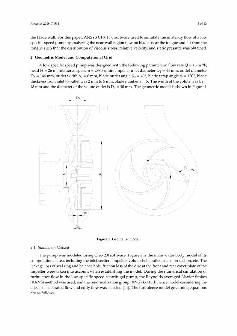
2.1. Simulation Method

The pump was modeled using Creo 2.0 software. Figure 2 is the main water body model of its computational area, including the inlet section, impeller, volute shell, outlet extension section, etc. The leakage loss of seal ring and balance hole, friction loss of the disc at the front and rear cover plate of the impeller were taken into account when establishing the model. During the numerical

Figure 1. Geometric model.

2.1. Simulation Method

The pump was modeled using Creo 2.0 software. Figure 2 is the main water body model of itscomputational area, including the inlet section, impeller, volute shell, outlet extension section, etc. Theleakage loss of seal ring and balance hole, friction loss of the disc at the front and rear cover plate of theimpeller were taken into account when establishing the model. During the numerical simulation ofturbulence flow in the low-specific-speed centrifugal pump, the Reynolds averaged Navier-Stokes(RANS) method was used, and the renormalization group (RNG) k-ε turbulence model considering theeffects of separated flow and eddy flow was selected [14]. The turbulence model governing equationsare as follows:

Processes 2019, 7, 514 4 of 13

∂∂t(ρk) +

∂∂xi

(ρkui) =∂∂x j

[(αεkµe f fµt

σk)∂k∂x j

] + Gk + Gb − ρε−YM + Sk (1)

∂∂t(ρε) +

∂∂xi

(ρεui) =∂∂x j

[(αεkµe f fµt

σk)∂ε∂x j

] + C1εεk(Gk + C3eGb) −C2ερ

ε2

k+ Sε (2)

Processes 2019, 7, x 4 of 13

simulation of turbulence flow in the low-specific-speed centrifugal pump, the Reynolds averaged Navier-Stokes (RANS) method was used, and the renormalization group (RNG) k-ε turbulence model considering the effects of separated flow and eddy flow was selected [14]. The turbulence model governing equations are as follows:

i( ) ( ) [( ) ]te ff k b M k

i j k j

kk ku k G G Y St x x xε

μρ ρ α μ ρεσ

∂ ∂ ∂ ∂+ = + + − − +∂ ∂ ∂ ∂

(1)

2

i 1 3 2( ) ( ) [( ) ] ( )te ff k e b

i j k j

u k C G C G C St x x x k kε ε ε ε

μ ε ε ερε ρε α μ ρσ

∂ ∂ ∂ ∂+ = + + − +∂ ∂ ∂ ∂

(2)

Compared with standard k-ε turbulence model, the rotation effect on αk and αε has been considered in the above formula, and the other terms have the same meaning as the standard k-ε turbulence model.

The boundary condition at the outlet was chosen as the pump’s flow rate, while the boundary condition at the inlet was chosen as the total pressure, and the reference pressure was set be 1.0 atm at the inlet. The walls formed by the impeller were defined as the rotating boundary and its rotating speed was 2880 r/min, the other walls were defined as the non-slip boundary, and the wall roughness was set to be 0.025 mm uniformly. Simulations were carried out using the commercial software ANSYS-CFX, the governing equations were discretized using the finite volume method, the pressure term was solved using the central difference scheme, the velocity term was solved using the second-order upwind difference scheme, the turbulent kinetic energy term and the turbulent energy dissipation rate term were solved using the second-order upwind difference scheme, and the near-wall flow was approximated using the standard wall function method. The convergence accuracy was set to 10−5. In this paper, unstructured tetrahedral meshes were used to divide the computational water domain. The grid independence of numerical simulation was studied under a design flow rate, and it was found that when the number of grids was more than 3.9 million, the fluctuation of the head and hydraulic efficiency was small, and the relative fluctuation range was less than 1%; therefore, it can be considered that the number of grids had no effect on the calculation results.

Figure 2. Water body model.

Compared with standard k-ε turbulence model, the rotation effect onαk andαε has been consideredin the above formula, and the other terms have the same meaning as the standard k-ε turbulence model.

The boundary condition at the outlet was chosen as the pump’s flow rate, while the boundarycondition at the inlet was chosen as the total pressure, and the reference pressure was set be 1.0atm at the inlet. The walls formed by the impeller were defined as the rotating boundary and itsrotating speed was 2880 r/min, the other walls were defined as the non-slip boundary, and the wallroughness was set to be 0.025 mm uniformly. Simulations were carried out using the commercialsoftware ANSYS-CFX, the governing equations were discretized using the finite volume method, thepressure term was solved using the central difference scheme, the velocity term was solved using thesecond-order upwind difference scheme, the turbulent kinetic energy term and the turbulent energydissipation rate term were solved using the second-order upwind difference scheme, and the near-wallflow was approximated using the standard wall function method. The convergence accuracy was setto 10−5. In this paper, unstructured tetrahedral meshes were used to divide the computational waterdomain. The grid independence of numerical simulation was studied under a design flow rate, and itwas found that when the number of grids was more than 3.9 million, the fluctuation of the head andhydraulic efficiency was small, and the relative fluctuation range was less than 1%; therefore, it can beconsidered that the number of grids had no effect on the calculation results.

Processes 2019, 7, 514 5 of 13

2.2. Experimental Method and Result

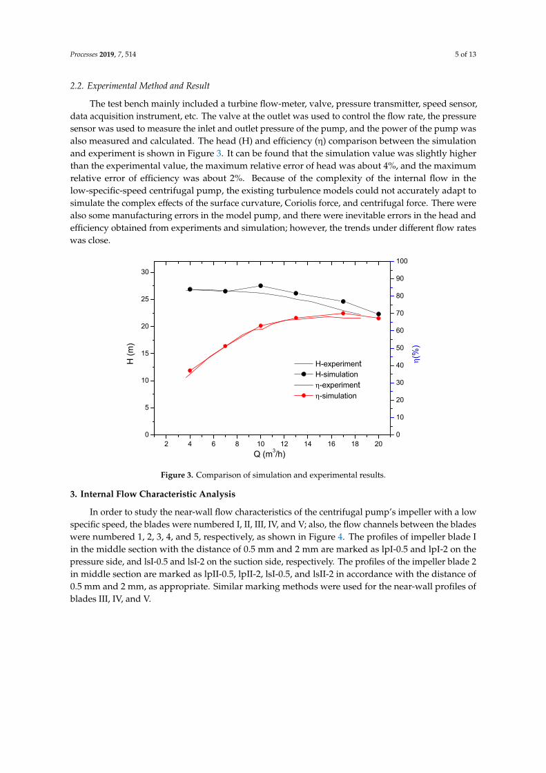
The test bench mainly included a turbine flow-meter, valve, pressure transmitter, speed sensor,data acquisition instrument, etc. The valve at the outlet was used to control the flow rate, the pressuresensor was used to measure the inlet and outlet pressure of the pump, and the power of the pump wasalso measured and calculated. The head (H) and efficiency (η) comparison between the simulationand experiment is shown in Figure 3. It can be found that the simulation value was slightly higherthan the experimental value, the maximum relative error of head was about 4%, and the maximumrelative error of efficiency was about 2%. Because of the complexity of the internal flow in thelow-specific-speed centrifugal pump, the existing turbulence models could not accurately adapt tosimulate the complex effects of the surface curvature, Coriolis force, and centrifugal force. There werealso some manufacturing errors in the model pump, and there were inevitable errors in the head andefficiency obtained from experiments and simulation; however, the trends under different flow rateswas close.

Processes 2019, 7, x 5 of 13

Figure 2. Water body model.

2.2. Experimental Method and Result

The test bench mainly included a turbine flow-meter, valve, pressure transmitter, speed sensor, data acquisition instrument, etc. The valve at the outlet was used to control the flow rate, the pressure sensor was used to measure the inlet and outlet pressure of the pump, and the power of the pump was also measured and calculated. The head (H) and efficiency (η) comparison between the simulation and experiment is shown in Figure 3. It can be found that the simulation value was slightly higher than the experimental value, the maximum relative error of head was about 4%, and the maximum relative error of efficiency was about 2%. Because of the complexity of the internal flow in the low-specific-speed centrifugal pump, the existing turbulence models could not accurately adapt to simulate the complex effects of the surface curvature, Coriolis force, and centrifugal force. There were also some manufacturing errors in the model pump, and there were inevitable errors in the head and efficiency obtained from experiments and simulation; however, the trends under different flow rates was close.

2 4 6 8 10 12 14 16 18 200

5

10

15

20

25

30

H-experiment H-simulation η-experiment η-simulation

Q (m3/h)

H (m

)

0

10

20

30

40

50

60

70

80

90

100

η(%

)

Figure 3. Comparison of simulation and experimental results.

3. Internal Flow Characteristic Analysis

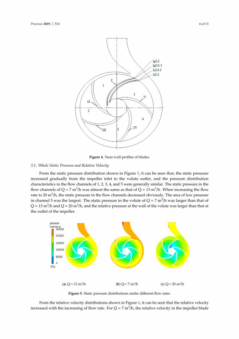
In order to study the near-wall flow characteristics of the centrifugal pump’s impeller with a low specific speed, the blades were numbered I, II, III, IV, and V; also, the flow channels between the blades were numbered 1, 2, 3, 4, and 5, respectively, as shown in Figure 4. The profiles of impeller blade I in the middle section with the distance of 0.5 mm and 2 mm are marked as lpI-0.5 and lpI-2 on the pressure side, and lsI-0.5 and lsI-2 on the suction side, respectively. The profiles of the impeller blade 2 in middle section are marked as lpII-0.5, lpII-2, lsI-0.5, and lsII-2 in accordance with the distance of 0.5 mm and 2 mm, as appropriate. Similar marking methods were used for the near-wall profiles of blades III, IV, and V.

Figure 3. Comparison of simulation and experimental results.

3. Internal Flow Characteristic Analysis

In order to study the near-wall flow characteristics of the centrifugal pump’s impeller with a lowspecific speed, the blades were numbered I, II, III, IV, and V; also, the flow channels between the bladeswere numbered 1, 2, 3, 4, and 5, respectively, as shown in Figure 4. The profiles of impeller blade Iin the middle section with the distance of 0.5 mm and 2 mm are marked as lpI-0.5 and lpI-2 on thepressure side, and lsI-0.5 and lsI-2 on the suction side, respectively. The profiles of the impeller blade 2in middle section are marked as lpII-0.5, lpII-2, lsI-0.5, and lsII-2 in accordance with the distance of0.5 mm and 2 mm, as appropriate. Similar marking methods were used for the near-wall profiles ofblades III, IV, and V.

Processes 2019, 7, 514 6 of 13Processes 2019, 7, x 6 of 13

Figure 4. Near-wall profiles of blades.

3.1. Whole Static Pressure and Relative Velocity

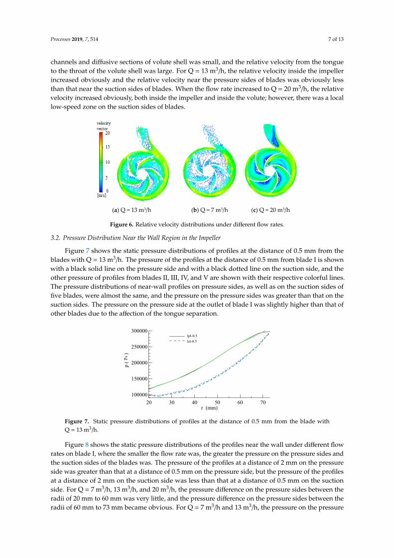
From the static pressure distribution shown in Figure 5, it can be seen that, the static pressure increased gradually from the impeller inlet to the volute outlet, and the pressure distribution characteristics in the flow channels of 1, 2, 3, 4, and 5 were generally similar. The static pressure in the flow channels of Q = 7 m3/h was almost the same as that of Q = 13 m3/h. When increasing the flow rate to 20 m3/h, the static pressure in the flow channels decreased obviously. The area of low pressure in channel 5 was the largest. The static pressure in the volute of Q = 7 m3/h was larger than that of Q = 13 m3/h and Q = 20 m3/h, and the relative pressure at the wall of the volute was larger than that at the outlet of the impeller.

(a) Q = 13 m3/h (b) Q = 7 m3/h (c) Q = 20 m3/h

Figure 5. Static pressure distributions under different flow rates.

Figure 4. Near-wall profiles of blades.

3.1. Whole Static Pressure and Relative Velocity

From the static pressure distribution shown in Figure 5, it can be seen that, the static pressureincreased gradually from the impeller inlet to the volute outlet, and the pressure distributioncharacteristics in the flow channels of 1, 2, 3, 4, and 5 were generally similar. The static pressure in theflow channels of Q = 7 m3/h was almost the same as that of Q = 13 m3/h. When increasing the flowrate to 20 m3/h, the static pressure in the flow channels decreased obviously. The area of low pressurein channel 5 was the largest. The static pressure in the volute of Q = 7 m3/h was larger than that ofQ = 13 m3/h and Q = 20 m3/h, and the relative pressure at the wall of the volute was larger than that atthe outlet of the impeller.

Processes 2019, 7, x 6 of 13

Figure 4. Near-wall profiles of blades.

3.1. Whole Static Pressure and Relative Velocity

From the static pressure distribution shown in Figure 5, it can be seen that, the static pressure increased gradually from the impeller inlet to the volute outlet, and the pressure distribution characteristics in the flow channels of 1, 2, 3, 4, and 5 were generally similar. The static pressure in the flow channels of Q = 7 m3/h was almost the same as that of Q = 13 m3/h. When increasing the flow rate to 20 m3/h, the static pressure in the flow channels decreased obviously. The area of low pressure in channel 5 was the largest. The static pressure in the volute of Q = 7 m3/h was larger than that of Q = 13 m3/h and Q = 20 m3/h, and the relative pressure at the wall of the volute was larger than that at the outlet of the impeller.

(a) Q = 13 m3/h (b) Q = 7 m3/h (c) Q = 20 m3/h

Figure 5. Static pressure distributions under different flow rates. Figure 5. Static pressure distributions under different flow rates.

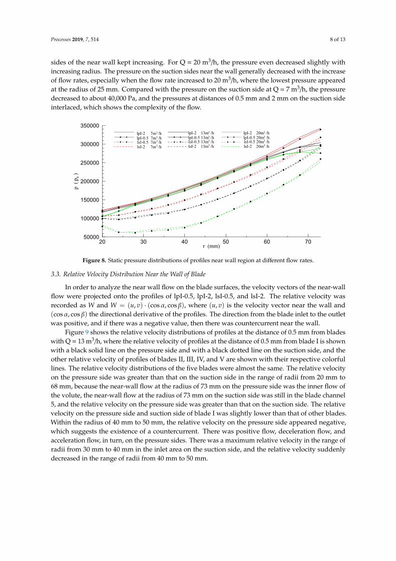
From the relative velocity distributions shown in Figure 6, it can be seen that the relative velocityincreased with the increasing of flow rate. For Q = 7 m3/h, the relative velocity in the impeller blade

Processes 2019, 7, 514 7 of 13

channels and diffusive sections of volute shell was small, and the relative velocity from the tongueto the throat of the volute shell was large. For Q = 13 m3/h, the relative velocity inside the impellerincreased obviously and the relative velocity near the pressure sides of blades was obviously lessthan that near the suction sides of blades. When the flow rate increased to Q = 20 m3/h, the relativevelocity increased obviously, both inside the impeller and inside the volute; however, there was a locallow-speed zone on the suction sides of blades.

Processes 2019, 7, x 7 of 13

From the relative velocity distributions shown in Figure 6, it can be seen that the relative velocity increased with the increasing of flow rate. For Q = 7 m3/h, the relative velocity in the impeller blade channels and diffusive sections of volute shell was small, and the relative velocity from the tongue to the throat of the volute shell was large. For Q = 13 m3/h, the relative velocity inside the impeller increased obviously and the relative velocity near the pressure sides of blades was obviously less than that near the suction sides of blades. When the flow rate increased to Q = 20 m3/h, the relative velocity increased obviously, both inside the impeller and inside the volute; however, there was a local low-speed zone on the suction sides of blades.

(a) Q = 13 m3/h (b) Q = 7 m3/h (c) Q = 20 m3/h

Figure 6. Relative velocity distributions under different flow rates.

3.2. Pressure Distribution Near the Wall Region in the Impeller

Figure 7 shows the static pressure distributions of profiles at the distance of 0.5 mm from the blades with Q = 13 m3/h. The pressure of the profiles at the distance of 0.5 mm from blade I is shown with a black solid line on the pressure side and with a black dotted line on the suction side, and the other pressure of profiles from blades II, III, IV, and V are shown with their respective colorful lines. The pressure distributions of near-wall profiles on pressure sides, as well as on the suction sides of five blades, were almost the same, and the pressure on the pressure sides was greater than that on the suction sides. The pressure on the pressure side at the outlet of blade I was slightly higher than that of other blades due to the affection of the tongue separation.

Figure 7. Static pressure distributions of profiles at the distance of 0.5 mm from the blade with Q = 13 m3/h.

Figure 8 shows the static pressure distributions of the profiles near the wall under different flow rates on blade I, where the smaller the flow rate was, the greater the pressure on the pressure sides and the suction sides of the blades was. The pressure of the profiles at a distance of 2 mm on the pressure side was greater than that at a distance of 0.5 mm on the pressure side, but the pressure of the profiles at a distance of 2 mm on the suction side was less than that at a distance of 0.5 mm on the suction side. For Q = 7 m3/h, 13 m3/h, and 20 m3/h, the pressure difference on the pressure sides between the radii of 20 mm to 60 mm was very little, and the pressure difference on the pressure sides between the radii of 60 mm to 73 mm became obvious. For Q = 7 m3/h and 13 m3/h, the pressure

r (mm)

p(

)

20 30 40 50 60 70100000

150000

200000

250000

300000

p a

lpI-0.5lsI-0.5

Figure 6. Relative velocity distributions under different flow rates.

3.2. Pressure Distribution Near the Wall Region in the Impeller

Figure 7 shows the static pressure distributions of profiles at the distance of 0.5 mm from theblades with Q = 13 m3/h. The pressure of the profiles at the distance of 0.5 mm from blade I is shownwith a black solid line on the pressure side and with a black dotted line on the suction side, and theother pressure of profiles from blades II, III, IV, and V are shown with their respective colorful lines.The pressure distributions of near-wall profiles on pressure sides, as well as on the suction sides offive blades, were almost the same, and the pressure on the pressure sides was greater than that on thesuction sides. The pressure on the pressure side at the outlet of blade I was slightly higher than that ofother blades due to the affection of the tongue separation.

Processes 2019, 7, x 7 of 13

From the relative velocity distributions shown in Figure 6, it can be seen that the relative velocity increased with the increasing of flow rate. For Q = 7 m3/h, the relative velocity in the impeller blade channels and diffusive sections of volute shell was small, and the relative velocity from the tongue to the throat of the volute shell was large. For Q = 13 m3/h, the relative velocity inside the impeller increased obviously and the relative velocity near the pressure sides of blades was obviously less than that near the suction sides of blades. When the flow rate increased to Q = 20 m3/h, the relative velocity increased obviously, both inside the impeller and inside the volute; however, there was a local low-speed zone on the suction sides of blades.

(a) Q = 13 m3/h (b) Q = 7 m3/h (c) Q = 20 m3/h

Figure 6. Relative velocity distributions under different flow rates.

3.2. Pressure Distribution Near the Wall Region in the Impeller

Figure 7 shows the static pressure distributions of profiles at the distance of 0.5 mm from the blades with Q = 13 m3/h. The pressure of the profiles at the distance of 0.5 mm from blade I is shown with a black solid line on the pressure side and with a black dotted line on the suction side, and the other pressure of profiles from blades II, III, IV, and V are shown with their respective colorful lines. The pressure distributions of near-wall profiles on pressure sides, as well as on the suction sides of five blades, were almost the same, and the pressure on the pressure sides was greater than that on the suction sides. The pressure on the pressure side at the outlet of blade I was slightly higher than that of other blades due to the affection of the tongue separation.

Figure 7. Static pressure distributions of profiles at the distance of 0.5 mm from the blade with Q = 13 m3/h.

Figure 8 shows the static pressure distributions of the profiles near the wall under different flow rates on blade I, where the smaller the flow rate was, the greater the pressure on the pressure sides and the suction sides of the blades was. The pressure of the profiles at a distance of 2 mm on the pressure side was greater than that at a distance of 0.5 mm on the pressure side, but the pressure of the profiles at a distance of 2 mm on the suction side was less than that at a distance of 0.5 mm on the suction side. For Q = 7 m3/h, 13 m3/h, and 20 m3/h, the pressure difference on the pressure sides between the radii of 20 mm to 60 mm was very little, and the pressure difference on the pressure sides between the radii of 60 mm to 73 mm became obvious. For Q = 7 m3/h and 13 m3/h, the pressure

r (mm)

p(

)

20 30 40 50 60 70100000

150000

200000

250000

300000

p a

lpI-0.5lsI-0.5

Figure 7. Static pressure distributions of profiles at the distance of 0.5 mm from the blade withQ = 13 m3/h.

Figure 8 shows the static pressure distributions of the profiles near the wall under different flowrates on blade I, where the smaller the flow rate was, the greater the pressure on the pressure sides andthe suction sides of the blades was. The pressure of the profiles at a distance of 2 mm on the pressureside was greater than that at a distance of 0.5 mm on the pressure side, but the pressure of the profilesat a distance of 2 mm on the suction side was less than that at a distance of 0.5 mm on the suctionside. For Q = 7 m3/h, 13 m3/h, and 20 m3/h, the pressure difference on the pressure sides between theradii of 20 mm to 60 mm was very little, and the pressure difference on the pressure sides between theradii of 60 mm to 73 mm became obvious. For Q = 7 m3/h and 13 m3/h, the pressure on the pressure

Processes 2019, 7, 514 8 of 13

sides of the near wall kept increasing. For Q = 20 m3/h, the pressure even decreased slightly withincreasing radius. The pressure on the suction sides near the wall generally decreased with the increaseof flow rates, especially when the flow rate increased to 20 m3/h, where the lowest pressure appearedat the radius of 25 mm. Compared with the pressure on the suction side at Q = 7 m3/h, the pressuredecreased to about 40,000 Pa, and the pressures at distances of 0.5 mm and 2 mm on the suction sideinterlaced, which shows the complexity of the flow.

Processes 2019, 7, x 8 of 13

on the pressure sides of the near wall kept increasing. For Q = 20 m3/h, the pressure even decreased slightly with increasing radius. The pressure on the suction sides near the wall generally decreased with the increase of flow rates, especially when the flow rate increased to 20 m3/h, where the lowest pressure appeared at the radius of 25 mm. Compared with the pressure on the suction side at Q = 7 m3/h, the pressure decreased to about 40,000 Pa, and the pressures at distances of 0.5 mm and 2 mm on the suction side interlaced, which shows the complexity of the flow.

Figure 8. Static pressure distributions of profiles near wall region at different flow rates.

3.3. Relative Velocity Distribution Near the Wall of Blade

In order to analyze the near wall flow on the blade surfaces, the velocity vectors of the near-wall flow were projected onto the profiles of lpI-0.5, lpI-2, lsI-0.5, and lsI-2. The relative velocity was recorded as W and )cos,(cos),( βα⋅= vuW , where ),( vu is the velocity vector near the wall and

)cos,(cos βα the directional derivative of the profiles. The direction from the blade inlet to the outlet was positive, and if there was a negative value, then there was countercurrent near the wall.

Figure 9 shows the relative velocity distributions of profiles at the distance of 0.5 mm from blades with Q = 13 m3/h, where the relative velocity of profiles at the distance of 0.5 mm from blade I is shown with a black solid line on the pressure side and with a black dotted line on the suction side, and the other relative velocity of profiles of blades II, III, IV, and V are shown with their respective colorful lines. The relative velocity distributions of the five blades were almost the same. The relative velocity on the pressure side was greater than that on the suction side in the range of radii from 20 mm to 68 mm, because the near-wall flow at the radius of 73 mm on the pressure side was the inner flow of the volute, the near-wall flow at the radius of 73 mm on the suction side was still in the blade channel 5, and the relative velocity on the pressure side was greater than that on the suction side. The relative velocity on the pressure side and suction side of blade I was slightly lower than that of other blades. Within the radius of 40 mm to 50 mm, the relative velocity on the pressure side appeared negative, which suggests the existence of a countercurrent. There was positive flow, deceleration flow, and acceleration flow, in turn, on the pressure sides. There was a maximum relative velocity in the range of radii from 30 mm to 40 mm in the inlet area on the suction side, and the relative velocity suddenly decreased in the range of radii from 40 mm to 50 mm.

r (mm)

p(

)

20 30 40 50 60 7050000

100000

150000

200000

250000

300000

350000

p

lpI-0.5 20m /hlpI-2 20m /h

lsI-2 20m /hlsI-0.5 20m /h

3

3

3

3lpI-0.5 7m /hlpI-2 7m /h

lsI-2 7m /hlsI-0.5 7m /h

3

3

3

3lpI-0.5 13m /hlpI-2 13m /h

lsI-2 13m /hlsI-0.5 13m /h

3

3

3

3

a

Figure 8. Static pressure distributions of profiles near wall region at different flow rates.

3.3. Relative Velocity Distribution Near the Wall of Blade

In order to analyze the near wall flow on the blade surfaces, the velocity vectors of the near-wallflow were projected onto the profiles of lpI-0.5, lpI-2, lsI-0.5, and lsI-2. The relative velocity wasrecorded as W and W = (u, v) · (cosα, cos β), where (u, v) is the velocity vector near the wall and(cosα, cos β) the directional derivative of the profiles. The direction from the blade inlet to the outletwas positive, and if there was a negative value, then there was countercurrent near the wall.

Figure 9 shows the relative velocity distributions of profiles at the distance of 0.5 mm from bladeswith Q = 13 m3/h, where the relative velocity of profiles at the distance of 0.5 mm from blade I is shownwith a black solid line on the pressure side and with a black dotted line on the suction side, and theother relative velocity of profiles of blades II, III, IV, and V are shown with their respective colorfullines. The relative velocity distributions of the five blades were almost the same. The relative velocityon the pressure side was greater than that on the suction side in the range of radii from 20 mm to68 mm, because the near-wall flow at the radius of 73 mm on the pressure side was the inner flow ofthe volute, the near-wall flow at the radius of 73 mm on the suction side was still in the blade channel5, and the relative velocity on the pressure side was greater than that on the suction side. The relativevelocity on the pressure side and suction side of blade I was slightly lower than that of other blades.Within the radius of 40 mm to 50 mm, the relative velocity on the pressure side appeared negative,which suggests the existence of a countercurrent. There was positive flow, deceleration flow, andacceleration flow, in turn, on the pressure sides. There was a maximum relative velocity in the range ofradii from 30 mm to 40 mm in the inlet area on the suction side, and the relative velocity suddenlydecreased in the range of radii from 40 mm to 50 mm.

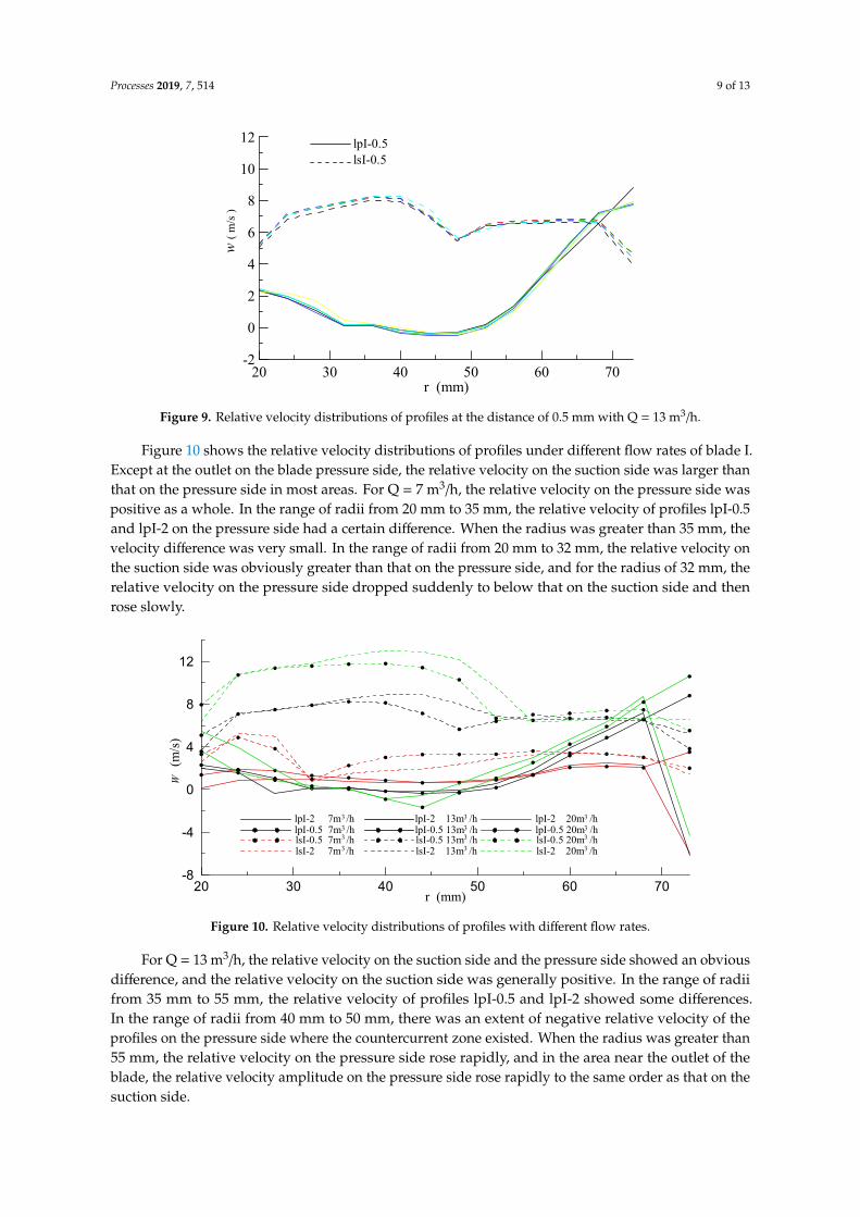
Processes 2019, 7, 514 9 of 13Processes 2019, 7, x 9 of 13

Figure 9. Relative velocity distributions of profiles at the distance of 0.5 mm with Q = 13 m3/h.

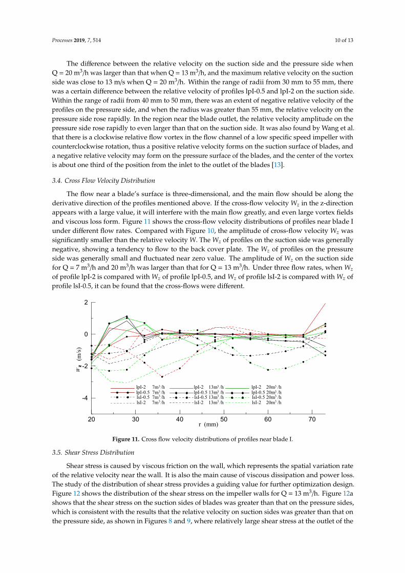
Figure 10 shows the relative velocity distributions of profiles under different flow rates of blade I. Except at the outlet on the blade pressure side, the relative velocity on the suction side was larger than that on the pressure side in most areas. For Q = 7 m3/h, the relative velocity on the pressure side was positive as a whole. In the range of radii from 20 mm to 35 mm, the relative velocity of profiles lpI-0.5 and lpI-2 on the pressure side had a certain difference. When the radius was greater than 35 mm, the velocity difference was very small. In the range of radii from 20 mm to 32 mm, the relative velocity on the suction side was obviously greater than that on the pressure side, and for the radius of 32 mm, the relative velocity on the pressure side dropped suddenly to below that on the suction side and then rose slowly.

For Q = 13 m3/h, the relative velocity on the suction side and the pressure side showed an obvious difference, and the relative velocity on the suction side was generally positive. In the range of radii from 35 mm to 55 mm, the relative velocity of profiles lpI-0.5 and lpI-2 showed some differences. In the range of radii from 40 mm to 50 mm, there was an extent of negative relative velocity of the profiles on the pressure side where the countercurrent zone existed. When the radius was greater than 55 mm, the relative velocity on the pressure side rose rapidly, and in the area near the outlet of the blade, the relative velocity amplitude on the pressure side rose rapidly to the same order as that on the suction side.

The difference between the relative velocity on the suction side and the pressure side when Q = 20 m3/h was larger than that when Q = 13 m3/h, and the maximum relative velocity on the suction side was close to 13 m/s when Q = 20 m3/h. Within the range of radii from 30 mm to 55 mm, there was a certain difference between the relative velocity of profiles lpI-0.5 and lpI-2 on the suction side. Within the range of radii from 40 mm to 50 mm, there was an extent of negative relative velocity of the profiles on the pressure side, and when the radius was greater than 55 mm, the relative velocity on the pressure side rose rapidly. In the region near the blade outlet, the relative velocity amplitude on the pressure side rose rapidly to even larger than that on the suction side. It was also found by Wang et al. that there is a clockwise relative flow vortex in the flow channel of a low specific speed impeller with counterclockwise rotation, thus a positive relative velocity forms on the suction surface of blades, and a negative relative velocity may form on the pressure surface of the blades, and the center of the vortex is about one third of the position from the inlet to the outlet of the blades [13].

r (mm)

w

20 30 40 50 60 70-2

0

2

4

6

8

10

12lsI-0.5lpI-0.5

(m/s)

Figure 9. Relative velocity distributions of profiles at the distance of 0.5 mm with Q = 13 m3/h.

Figure 10 shows the relative velocity distributions of profiles under different flow rates of blade I.Except at the outlet on the blade pressure side, the relative velocity on the suction side was larger thanthat on the pressure side in most areas. For Q = 7 m3/h, the relative velocity on the pressure side waspositive as a whole. In the range of radii from 20 mm to 35 mm, the relative velocity of profiles lpI-0.5and lpI-2 on the pressure side had a certain difference. When the radius was greater than 35 mm, thevelocity difference was very small. In the range of radii from 20 mm to 32 mm, the relative velocity onthe suction side was obviously greater than that on the pressure side, and for the radius of 32 mm, therelative velocity on the pressure side dropped suddenly to below that on the suction side and thenrose slowly.Processes 2019, 7, x 10 of 13

Figure 10. Relative velocity distributions of profiles with different flow rates.

3.4. Cross Flow Velocity Distribution

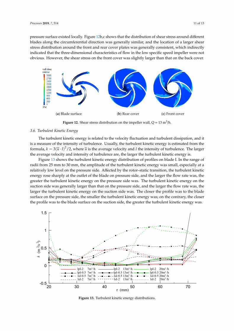
The flow near a blade’s surface is three-dimensional, and the main flow should be along the derivative direction of the profiles mentioned above. If the cross-flow velocity zW in the z-direction appears with a large value, it will interfere with the main flow greatly, and even large vortex fields and viscous loss form. Figure 11 shows the cross-flow velocity distributions of profiles near blade I under different flow rates. Compared with Figure 10, the amplitude of cross-flow velocity zW was significantly smaller than the relative velocity W. The zW of profiles on the suction side was generally negative, showing a tendency to flow to the back cover plate. The zW of profiles on the pressure side was generally small and fluctuated near zero value. The amplitude of zW on the suction side for Q = 7 m3/h and 20 m3/h was larger than that for Q = 13 m3/h. Under three flow rates, when zW of profile lpI-2 is compared with zW of profile lpI-0.5, and zW of profile lsI-2 is compared with zW of profile lsI-0.5, it can be found that the cross-flows were different.

Figure 11. Cross flow velocity distributions of profiles near blade I.

3.5. Shear Stress Distribution

Shear stress is caused by viscous friction on the wall, which represents the spatial variation rate of the relative velocity near the wall. It is also the main cause of viscous dissipation and power loss. The study of the distribution of shear stress provides a guiding value for further optimization design. Figure 12 shows the distribution of the shear stress on the impeller walls for Q = 13 m3/h. Figure 12a shows that the shear stress on the suction sides of blades was greater than that on the pressure sides,

r (mm)

(m/s)

20 30 40 50 60 70-8

-4

0

4

8

12

lpI-0.5 20m /hlpI-2 20m /h

lsI-2 20m /hlsI-0.5 20m /h

3

3

3

3lpI-0.5 7m /hlpI-2 7m /h

lsI-2 7m /hlsI-0.5 7m /h

3

3

3

3lpI-0.5 13m /hlpI-2 13m /h

lsI-2 13m /hlsI-0.5 13m /h

3

3

3

3

W

r (mm)

(m/s)

20 30 40 50 60 70

-4

-2

0

2

lpI-0.5 20m /hlpI-2 20m /h

lsI-2 20m /hlsI-0.5 20m /h

3

3

3

3lpI-0.5 7m /hlpI-2 7m /h

lsI-2 7m /hlsI-0.5 7m /h

3

3

3

3lpI-0.5 13m /hlpI-2 13m /h

lsI-2 13m /hlsI-0.5 13m /h

3

3

3

3

zW

Figure 10. Relative velocity distributions of profiles with different flow rates.

For Q = 13 m3/h, the relative velocity on the suction side and the pressure side showed an obviousdifference, and the relative velocity on the suction side was generally positive. In the range of radiifrom 35 mm to 55 mm, the relative velocity of profiles lpI-0.5 and lpI-2 showed some differences.In the range of radii from 40 mm to 50 mm, there was an extent of negative relative velocity of theprofiles on the pressure side where the countercurrent zone existed. When the radius was greater than55 mm, the relative velocity on the pressure side rose rapidly, and in the area near the outlet of theblade, the relative velocity amplitude on the pressure side rose rapidly to the same order as that on thesuction side.

Processes 2019, 7, 514 10 of 13

The difference between the relative velocity on the suction side and the pressure side whenQ = 20 m3/h was larger than that when Q = 13 m3/h, and the maximum relative velocity on the suctionside was close to 13 m/s when Q = 20 m3/h. Within the range of radii from 30 mm to 55 mm, therewas a certain difference between the relative velocity of profiles lpI-0.5 and lpI-2 on the suction side.Within the range of radii from 40 mm to 50 mm, there was an extent of negative relative velocity of theprofiles on the pressure side, and when the radius was greater than 55 mm, the relative velocity on thepressure side rose rapidly. In the region near the blade outlet, the relative velocity amplitude on thepressure side rose rapidly to even larger than that on the suction side. It was also found by Wang et al.that there is a clockwise relative flow vortex in the flow channel of a low specific speed impeller withcounterclockwise rotation, thus a positive relative velocity forms on the suction surface of blades, anda negative relative velocity may form on the pressure surface of the blades, and the center of the vortexis about one third of the position from the inlet to the outlet of the blades [13].

3.4. Cross Flow Velocity Distribution

The flow near a blade’s surface is three-dimensional, and the main flow should be along thederivative direction of the profiles mentioned above. If the cross-flow velocity Wz in the z-directionappears with a large value, it will interfere with the main flow greatly, and even large vortex fieldsand viscous loss form. Figure 11 shows the cross-flow velocity distributions of profiles near blade Iunder different flow rates. Compared with Figure 10, the amplitude of cross-flow velocity Wz wassignificantly smaller than the relative velocity W. The Wz of profiles on the suction side was generallynegative, showing a tendency to flow to the back cover plate. The Wz of profiles on the pressureside was generally small and fluctuated near zero value. The amplitude of Wz on the suction sidefor Q = 7 m3/h and 20 m3/h was larger than that for Q = 13 m3/h. Under three flow rates, when Wz

of profile lpI-2 is compared with Wz of profile lpI-0.5, and Wz of profile lsI-2 is compared with Wz ofprofile lsI-0.5, it can be found that the cross-flows were different.

Processes 2019, 7, x 10 of 13

Figure 10. Relative velocity distributions of profiles with different flow rates.

3.4. Cross Flow Velocity Distribution

The flow near a blade’s surface is three-dimensional, and the main flow should be along the derivative direction of the profiles mentioned above. If the cross-flow velocity zW in the z-direction appears with a large value, it will interfere with the main flow greatly, and even large vortex fields and viscous loss form. Figure 11 shows the cross-flow velocity distributions of profiles near blade I under different flow rates. Compared with Figure 10, the amplitude of cross-flow velocity zW was significantly smaller than the relative velocity W. The zW of profiles on the suction side was generally negative, showing a tendency to flow to the back cover plate. The zW of profiles on the pressure side was generally small and fluctuated near zero value. The amplitude of zW on the suction side for Q = 7 m3/h and 20 m3/h was larger than that for Q = 13 m3/h. Under three flow rates, when zW of profile lpI-2 is compared with zW of profile lpI-0.5, and zW of profile lsI-2 is compared with zW of profile lsI-0.5, it can be found that the cross-flows were different.

Figure 11. Cross flow velocity distributions of profiles near blade I.

3.5. Shear Stress Distribution

Shear stress is caused by viscous friction on the wall, which represents the spatial variation rate of the relative velocity near the wall. It is also the main cause of viscous dissipation and power loss. The study of the distribution of shear stress provides a guiding value for further optimization design. Figure 12 shows the distribution of the shear stress on the impeller walls for Q = 13 m3/h. Figure 12a shows that the shear stress on the suction sides of blades was greater than that on the pressure sides,

r (mm)

(m/s)

20 30 40 50 60 70-8

-4

0

4

8

12

lpI-0.5 20m /hlpI-2 20m /h

lsI-2 20m /hlsI-0.5 20m /h

3

3

3

3lpI-0.5 7m /hlpI-2 7m /h

lsI-2 7m /hlsI-0.5 7m /h

3

3

3

3lpI-0.5 13m /hlpI-2 13m /h

lsI-2 13m /hlsI-0.5 13m /h

3

3

3

3

W

r (mm)

(m/s)

20 30 40 50 60 70

-4

-2

0

2

lpI-0.5 20m /hlpI-2 20m /h

lsI-2 20m /hlsI-0.5 20m /h

3

3

3

3lpI-0.5 7m /hlpI-2 7m /h

lsI-2 7m /hlsI-0.5 7m /h

3

3

3

3lpI-0.5 13m /hlpI-2 13m /h

lsI-2 13m /hlsI-0.5 13m /h

3

3

3

3

zW

Figure 11. Cross flow velocity distributions of profiles near blade I.

3.5. Shear Stress Distribution

Shear stress is caused by viscous friction on the wall, which represents the spatial variation rateof the relative velocity near the wall. It is also the main cause of viscous dissipation and power loss.The study of the distribution of shear stress provides a guiding value for further optimization design.Figure 12 shows the distribution of the shear stress on the impeller walls for Q = 13 m3/h. Figure 12ashows that the shear stress on the suction sides of blades was greater than that on the pressure sides,which is consistent with the results that the relative velocity on suction sides was greater than that onthe pressure side, as shown in Figures 8 and 9, where relatively large shear stress at the outlet of the

Processes 2019, 7, 514 11 of 13

pressure surface existed locally. Figure 12b,c shows that the distribution of shear stress around differentblades along the circumferential direction was generally similar, and the location of a larger shearstress distribution around the front and rear cover plates was generally consistent, which indirectlyindicated that the three-dimensional characteristics of flow in the low specific speed impeller were notobvious. However, the shear stress on the front cover was slightly larger than that on the back cover.

Processes 2019, 7, x 11 of 13

which is consistent with the results that the relative velocity on suction sides was greater than that on the pressure side, as shown in Figures 8 and 9, where relatively large shear stress at the outlet of the pressure surface existed locally. Figure 12b,c shows that the distribution of shear stress around different blades along the circumferential direction was generally similar, and the location of a larger shear stress distribution around the front and rear cover plates was generally consistent, which indirectly indicated that the three-dimensional characteristics of flow in the low specific speed impeller were not obvious. However, the shear stress on the front cover was slightly larger than that on the back cover.

(a) Blade surface (b) Rear cover (c) Front cover

Figure 12. Shear stress distribution on the impeller wall, Q = 13 m3/h.

3.6. Turbulent Kinetic Energy

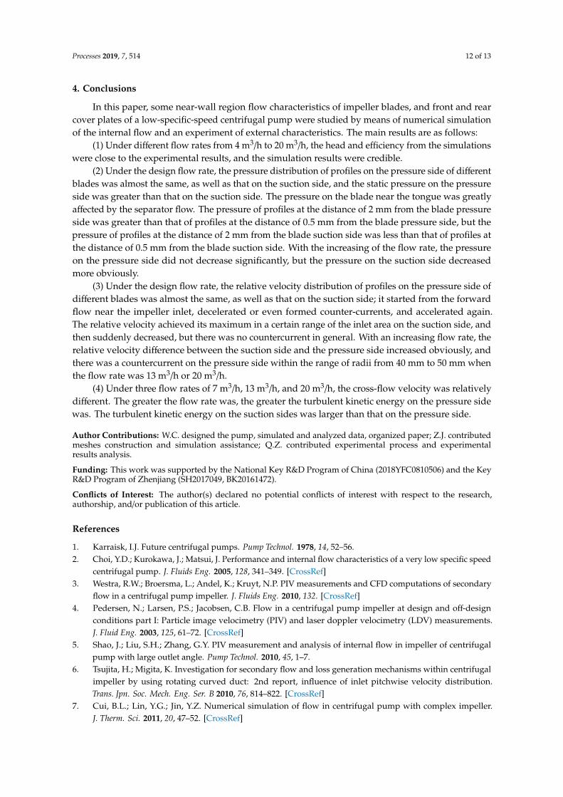
The turbulent kinetic energy is related to the velocity fluctuation and turbulent dissipation, and it is a measure of the intensity of turbulence. Usually, the turbulent kinetic energy is estimated from the formula, 2/)(3 2Iuk ⋅= , where u is the average velocity and I the intensity of turbulence. The larger the average velocity and intensity of turbulence are, the larger the turbulent kinetic energy is.

Figure 13 shows the turbulent kinetic energy distribution of profiles on blade I. In the range of radii from 25 mm to 30 mm, the amplitude of the turbulent kinetic energy was small, especially at a relatively low level on the pressure side. Affected by the rotor–static transition, the turbulent kinetic energy rose sharply at the outlet of the blade on pressure side, and the larger the flow rate was, the greater the turbulent kinetic energy on the pressure side was. The turbulent kinetic energy on the suction side was generally larger than that on the pressure side, and the larger the flow rate was, the larger the turbulent kinetic energy on the suction side was. The closer the profile was to the blade surface on the pressure side, the smaller the turbulent kinetic energy was; on the contrary, the closer the profile was to the blade surface on the suction side, the greater the turbulent kinetic energy was.

r(mm)

k(m

/s)

20 30 40 50 60 70-0.5

0

0.5

1

1.5

lpI-0.5 20m /hlpI-2 20m /h

lsI-2 20m /hlsI-0.5 20m /h

3

3

3

3lpI-0.5 7m /hlpI-2 7m /h

lsI-2 7m /hlsI-0.5 7m /h

3

3

3

3lpI-0.5 13m /hlpI-2 13m /h

lsI-2 13m /hlsI-0.5 13m /h

3

3

3

3

2

r (mm)

(m/s)

20 30 40 50 60 70-0.5

0

0.5

1

1.5

lpI-0.5 20m /hlpI-2 20m /h

lsI-2 20m /hlsI-0.5 20m /h

3

3

3

3lpI-0.5 7m /hlpI-2 7m /h

lsI-2 7m /hlsI-0.5 7m /h

3

3

3

3lpI-0.5 13m /hlpI-2 13m /h

lsI-2 13m /hlsI-0.5 13m /h

3

3

3

3

22

k

Figure 12. Shear stress distribution on the impeller wall, Q = 13 m3/h.

3.6. Turbulent Kinetic Energy

The turbulent kinetic energy is related to the velocity fluctuation and turbulent dissipation, and itis a measure of the intensity of turbulence. Usually, the turbulent kinetic energy is estimated from theformula, k = 3(u · I)2/2, where u is the average velocity and I the intensity of turbulence. The largerthe average velocity and intensity of turbulence are, the larger the turbulent kinetic energy is.

Figure 13 shows the turbulent kinetic energy distribution of profiles on blade I. In the range ofradii from 25 mm to 30 mm, the amplitude of the turbulent kinetic energy was small, especially at arelatively low level on the pressure side. Affected by the rotor–static transition, the turbulent kineticenergy rose sharply at the outlet of the blade on pressure side, and the larger the flow rate was, thegreater the turbulent kinetic energy on the pressure side was. The turbulent kinetic energy on thesuction side was generally larger than that on the pressure side, and the larger the flow rate was, thelarger the turbulent kinetic energy on the suction side was. The closer the profile was to the bladesurface on the pressure side, the smaller the turbulent kinetic energy was; on the contrary, the closerthe profile was to the blade surface on the suction side, the greater the turbulent kinetic energy was.

Processes 2019, 7, x 11 of 13

which is consistent with the results that the relative velocity on suction sides was greater than that on the pressure side, as shown in Figures 8 and 9, where relatively large shear stress at the outlet of the pressure surface existed locally. Figure 12b,c shows that the distribution of shear stress around different blades along the circumferential direction was generally similar, and the location of a larger shear stress distribution around the front and rear cover plates was generally consistent, which indirectly indicated that the three-dimensional characteristics of flow in the low specific speed impeller were not obvious. However, the shear stress on the front cover was slightly larger than that on the back cover.

(a) Blade surface (b) Rear cover (c) Front cover

Figure 12. Shear stress distribution on the impeller wall, Q = 13 m3/h.

3.6. Turbulent Kinetic Energy

The turbulent kinetic energy is related to the velocity fluctuation and turbulent dissipation, and it is a measure of the intensity of turbulence. Usually, the turbulent kinetic energy is estimated from the formula, 2/)(3 2Iuk ⋅= , where u is the average velocity and I the intensity of turbulence. The larger the average velocity and intensity of turbulence are, the larger the turbulent kinetic energy is.

Figure 13 shows the turbulent kinetic energy distribution of profiles on blade I. In the range of radii from 25 mm to 30 mm, the amplitude of the turbulent kinetic energy was small, especially at a relatively low level on the pressure side. Affected by the rotor–static transition, the turbulent kinetic energy rose sharply at the outlet of the blade on pressure side, and the larger the flow rate was, the greater the turbulent kinetic energy on the pressure side was. The turbulent kinetic energy on the suction side was generally larger than that on the pressure side, and the larger the flow rate was, the larger the turbulent kinetic energy on the suction side was. The closer the profile was to the blade surface on the pressure side, the smaller the turbulent kinetic energy was; on the contrary, the closer the profile was to the blade surface on the suction side, the greater the turbulent kinetic energy was.

r(mm)

k(m

/s)

20 30 40 50 60 70-0.5

0

0.5

1

1.5

lpI-0.5 20m /hlpI-2 20m /h

lsI-2 20m /hlsI-0.5 20m /h

3

3

3

3lpI-0.5 7m /hlpI-2 7m /h

lsI-2 7m /hlsI-0.5 7m /h

3

3

3

3lpI-0.5 13m /hlpI-2 13m /h

lsI-2 13m /hlsI-0.5 13m /h

3

3

3

3

2

r (mm)

(m/s)

20 30 40 50 60 70-0.5

0

0.5

1

1.5

lpI-0.5 20m /hlpI-2 20m /h

lsI-2 20m /hlsI-0.5 20m /h

3

3

3

3lpI-0.5 7m /hlpI-2 7m /h

lsI-2 7m /hlsI-0.5 7m /h

3

3

3

3lpI-0.5 13m /hlpI-2 13m /h

lsI-2 13m /hlsI-0.5 13m /h

3

3

3

3

22

k

Figure 13. Turbulent kinetic energy distributions.

Processes 2019, 7, 514 12 of 13

4. Conclusions

In this paper, some near-wall region flow characteristics of impeller blades, and front and rearcover plates of a low-specific-speed centrifugal pump were studied by means of numerical simulationof the internal flow and an experiment of external characteristics. The main results are as follows:

(1) Under different flow rates from 4 m3/h to 20 m3/h, the head and efficiency from the simulationswere close to the experimental results, and the simulation results were credible.

(2) Under the design flow rate, the pressure distribution of profiles on the pressure side of differentblades was almost the same, as well as that on the suction side, and the static pressure on the pressureside was greater than that on the suction side. The pressure on the blade near the tongue was greatlyaffected by the separator flow. The pressure of profiles at the distance of 2 mm from the blade pressureside was greater than that of profiles at the distance of 0.5 mm from the blade pressure side, but thepressure of profiles at the distance of 2 mm from the blade suction side was less than that of profiles atthe distance of 0.5 mm from the blade suction side. With the increasing of the flow rate, the pressureon the pressure side did not decrease significantly, but the pressure on the suction side decreasedmore obviously.

(3) Under the design flow rate, the relative velocity distribution of profiles on the pressure side ofdifferent blades was almost the same, as well as that on the suction side; it started from the forwardflow near the impeller inlet, decelerated or even formed counter-currents, and accelerated again.The relative velocity achieved its maximum in a certain range of the inlet area on the suction side, andthen suddenly decreased, but there was no countercurrent in general. With an increasing flow rate, therelative velocity difference between the suction side and the pressure side increased obviously, andthere was a countercurrent on the pressure side within the range of radii from 40 mm to 50 mm whenthe flow rate was 13 m3/h or 20 m3/h.

(4) Under three flow rates of 7 m3/h, 13 m3/h, and 20 m3/h, the cross-flow velocity was relativelydifferent. The greater the flow rate was, the greater the turbulent kinetic energy on the pressure sidewas. The turbulent kinetic energy on the suction sides was larger than that on the pressure side.

Author Contributions: W.C. designed the pump, simulated and analyzed data, organized paper; Z.J. contributedmeshes construction and simulation assistance; Q.Z. contributed experimental process and experimentalresults analysis.

Funding: This work was supported by the National Key R&D Program of China (2018YFC0810506) and the KeyR&D Program of Zhenjiang (SH2017049, BK20161472).

Conflicts of Interest: The author(s) declared no potential conflicts of interest with respect to the research,authorship, and/or publication of this article.

References

1. Karraisk, I.J. Future centrifugal pumps. Pump Technol. 1978, 14, 52–56.2. Choi, Y.D.; Kurokawa, J.; Matsui, J. Performance and internal flow characteristics of a very low specific speed

centrifugal pump. J. Fluids Eng. 2005, 128, 341–349. [CrossRef]3. Westra, R.W.; Broersma, L.; Andel, K.; Kruyt, N.P. PIV measurements and CFD computations of secondary

flow in a centrifugal pump impeller. J. Fluids Eng. 2010, 132. [CrossRef]4. Pedersen, N.; Larsen, P.S.; Jacobsen, C.B. Flow in a centrifugal pump impeller at design and off-design

conditions part I: Particle image velocimetry (PIV) and laser doppler velocimetry (LDV) measurements.J. Fluid Eng. 2003, 125, 61–72. [CrossRef]

5. Shao, J.; Liu, S.H.; Zhang, G.Y. PIV measurement and analysis of internal flow in impeller of centrifugalpump with large outlet angle. Pump Technol. 2010, 45, 1–7.

6. Tsujita, H.; Migita, K. Investigation for secondary flow and loss generation mechanisms within centrifugalimpeller by using rotating curved duct: 2nd report, influence of inlet pitchwise velocity distribution.Trans. Jpn. Soc. Mech. Eng. Ser. B 2010, 76, 814–822. [CrossRef]

7. Cui, B.L.; Lin, Y.G.; Jin, Y.Z. Numerical simulation of flow in centrifugal pump with complex impeller.J. Therm. Sci. 2011, 20, 47–52. [CrossRef]

Processes 2019, 7, 514 13 of 13

8. Limbach, P.; Skoda, R. Numerical and experimental analysis of cavitating flow in a low specific speedcentrifugal pump with different surface roughness. J. Fluids Eng. 2017, 139. [CrossRef]

9. Cao, W.D.; Yao, L.J.; Liu, B.; Zhang, Y. The influence of impeller eccentricity on centrifugal pump. Adv. Mech.Eng. 2017, 9. [CrossRef]

10. Zhang, Y.L.; Zhu, Z.C.; Li, W.G.; Xiao, J.J. Effects of viscosity on transient behavior of a low specific speedcentrifugal pump in starting and stopping periods. Int. J. Fluid Mech. Res. 2018, 45, 1–20. [CrossRef]

11. Chen, J.; Wang, Y.; Liu, H.L.; Shao, C.; Zhang, X. Internal flow and analysis of its unsteady characteristics incentrifugal pump with ultra-low specific-speed. J. Drain. Irrig. Mach. Eng. 2018, 36, 377–383.

12. Dong, L.; Zhao, Y.Q.; Liu, H.L.; Dai, C. The effect of front streamline wrapping angle variation in a super-lowspecific speed centrifugal pump. Proc. Inst. Mech. Eng. Part. C: J. Mech. Eng. Sci. 2018, 232. [CrossRef]

13. Zhang, R.H.; Chen, X.B.; Guo, G.Q.; Li, R. Reconstruction and modal analysis for flow field of low Specificspeed centrifugal pump impeller. Trans. Chin. Soc. Agric. Mach. 2018, 49, 143–149.

14. Wang, C.; Zhang, Y.X.; Li, Z.W.; Xu, A.; Xu, C.; Shi, Z. Pressure fluctuation-vortex interaction in an ultra-lowspecific-speed centrifugal pump. J. Low Freq. Noise Vib. Act. Control. 2019, 38, 527–543. [CrossRef]

© 2019 by the authors. Licensee MDPI, Basel, Switzerland. This article is an open accessarticle distributed under the terms and conditions of the Creative Commons Attribution(CC BY) license (http://creativecommons.org/licenses/by/4.0/).