Impacts of Transportation Investment on Real Property Values:

An Analysis with Spatial Hedonic Price Models

by

Kihwan Seo

A Dissertation Presented in Partial Fulfillment

of the Requirements for the Degree

Doctor of Philosophy

Approved April 2016 by the

Graduate Supervisory Committee:

Michael Kuby, Chair

Aaron Golub

Deborah Salon

ARIZONA STATE UNIVERSITY

May 2016

i

ABSTRACT

Transportation infrastructure in urban areas has significant impacts on socio-

economic activities, land use, and real property values. This dissertation proposes a more

comprehensive theory of the positive and negative relationships between property values

and transportation investments that distinguishes different effects by mode (rail vs. road),

by network component (nodes vs. links), and by distance from them. It hypothesizes that

transportation investment generates improvement in accessibility that accrue only to the

nodes such as highway exits and light rail stations. Simultaneously, it tests the hypothesis

that both transport nodes and links emanate short-distance negative nuisance effects due

to disamenities such as traffic and noise. It also tests the hypothesis that nodes of both

modes generate a net effect combining accessibility and disamenities. For highways, the

configuration at grade or above/below ground is also tested. In addition, this dissertation

hypothesizes that the condition of road pavement may have an impact on residential

property values adjacent to the road segments. As pavement condition improves, value of

properties adjacent to a road are hypothesized to increase as well. A multiple-distance-

bands approach is used to capture distance decay of amenities and disamenities from

nodes and links; and pavement condition index (PCI) is used to test the relationship

between road condition and residential property values. The hypotheses are tested using

spatial hedonic models that are specific to each of residential and commercial property

market. Results confirm that proximity to transport nodes are associated positively with

both residential and commercial property values. As a function of distance from highway

exits and light rail transit (LRT) stations, the distance-band coefficients form a

conventional distance decay curve. However, contrary to our hypotheses, no net effect is

ii

evident. The accessibility effect for highway exits extends farther than for LRT stations

in residential model as expected. The highway configuration effect on residential home

values confirms that below-grade highways have relatively positive impacts on nearby

houses compared to those at ground level or above. Lastly, results for the relationship

between pavement condition and residential home values show that there is no significant

effect between them.

Some differences in the effect of infrastructure on property values emerge

between residential and commercial markets. In the commercial models, the accessibility

effect for highway exits extends less than for LRT stations. Though coefficients for short

distances (within 300m) from highways and LRT links were expected to be negative in

both residential and commercial models, only commercial models show a significant

negative relationship. Different effects by mode, network component, and distance on

commercial submarkets (i.e., industrial, office, retail and service properties) are tested as

well and the results vary based on types of submarket.

Consequently, findings of three individual paper confirm that transportation

investments mostly have significant impacts on real-estate properties either in a positive

or negative direction in accordance with the transport mode, network component, and

distance, though effects for some conditions (e.g., proximity to links of highway and light

rail, and pavement quality) do not significantly change home values. Results can be used

for city authorities and planners for funding mechanisms of transport infrastructure or

validity of investments as well as private developers for maximizing development profits

or for locating developments.

iii

TABLE OF CONTENTS

Page

LIST OF TABLES ................................................................................................................... vi

LIST OF FIGURES ............................................................................................................... vii

CHAPTER

1 INTRODUCTION ................. ................................................................................. 1

Overview ..................................................................................................... 1

Problem Statement: Research Questions and Hypotheses ......................... 3

Significance ................................................................................................. 5

Dissertation Structure .................................................................................. 6

2 IMPACTS OF HIGHWAYS AND LIGHT RAIL TRANSIT ON RESIDENTIAL

PROPERTY VALUES ............................................................................................ 7

Introduction ................................................................................................. 8

Literature Review ........................................................................................ 9

Theoretical Model ..................................................................................... 14

Methods ..................................................................................................... 17

Study Area and Data ................................................................................. 20

Results........................................................................................................ 25

Conclusions ............................................................................................... 31

3 IMPACTS OF HIGHWAYS AND LIGHT RAIL TRANSIT ON

COMMERCIAL PROPERTY VALUES ............................................................ 35

Introduction ............................................................................................... 36

Literature Review ...................................................................................... 37

iv

CHAPTER Page

Theoretical Framework ............................................................................. 43

Methods ..................................................................................................... 46

Study Area and Data ................................................................................. 48

Results........................................................................................................ 54

Conclusions ............................................................................................... 63

4 PAVEMENT CONDITION AND PROPERTY VALUES .................................. 66

Introduction ............................................................................................... 67

Literature Review ...................................................................................... 68

Study Area and Data ................................................................................. 74

Methods ..................................................................................................... 81

Results........................................................................................................ 83

Disscussion and Conclusions .................................................................... 90

5 CONCLUSIONS .................. ................................................................................. 92

Overview ................................................................................................... 92

Implications ............................................................................................... 93

Future Research ......................................................................................... 94

REFERENCES ....... ............................................................................................................... 97

APPENDIX

A SUMMARY OF MAIN VARIABLES ............................................................... 105

B SUMMARY OF SELECTED LITERATURE ON ROAD AND RAIL

IMPACTS IN HEDONIC PRICE MODELS FOR COMMERCIAL

PROPERTIES ....................................................................................................... 108

v

APPENDIX Page

C ESTIMATION RESULTS FOR THE WHOLE COMMERCIAL

PROPERTIES.. ..................................................................................................... 111

D ESTIMATION RESULTS FOR THE INDUSTRIAL PROPERTIES ............. 113

E ESTIMATION RESULTS FOR THE OFFICE PROPERTIES ........................ 115

F ESTIMATION RESULTS FOR RETAIL AND SERVICE PROPERTIES .... 117

G DETAILED RESULTS FOR VALLEJO ........................................................... 119

H DETAILED RESULTS FOR VACAVILLE ...................................................... 121

I DETAILED RESULTS FOR FAIRFIELD ......................................................... 123

J DETAILED RESULTS FOR SUISUN CITY .................................................... 125

K DETAILED RESULTS FOR BENICIA ............................................................. 127

L DETAILED RESULTS FOR DIXON ................................................................ 129

M DETAILED RESULTS FOR RIO VISTA ......................................................... 131

N DETAILED RESULTS FOR SOLANO COUNTY ........................................... 133

vi

LIST OF TABLES

Table Page

1. Summary of Selected Literature on Road and Rail Impacts in Hedonic Price..... 10

2. Estimation Results........ ......................................................................................... 26

3. Summary of Main Variables (Observations = 3,642) ......................................... 52

4. Percentage of Observations in Distance Dummy Variables ................................. 53

5. Estimation Results of Commercial Markets ......................................................... 55

6. List of Data Provided ............................................................................................ 75

7. Descriptive Statistics of Main Variables (N = 19,608) ....................................... 78

8. Percent of Observations for Each City and Year ................................................. 79

9. Estimation Results of All Properties (N = 19,608) .............................................. 85

10. Estimation Results of the Properties with Surveyed PCI (N = 5,121) ................ 88

11. Estimation Results of Cities ................................................................................. 90

vii

LIST OF FIGURES

Figure Page

1. Conceptual Framework for Net Benefit of Combined Impacts of

Accessibility and Disamenity ........................................................................ 17

2. Key Dataset Used for Extracting Explanatory Variables for Hedonic

Regression ...................................................................................................... 22

3. Phoenix Land Cover Classification Map Using Quickbird Imageries

(Source: Central Arizona-Phoenix Long-Term Ecological Research (CAP

LTER), National Science Foundation Grant No. BCS-1026865)................. 24

4. Coefficients of Distance from the Highway Exit ........................................... 29

5 Coefficients of Distance from the Light Rail Station .................................... 30

6. Conceptual Framework for Net Benefit of Combined Impacts of

Accessibility and Disamenities (Source: Seo et al., 2014 - Modified for

Commercial Property) .................................................................................... 44

7. Study Area and Distribution of All Commercial Properties ........................ 51

8. Map of Multiple Distance Band Approach. Black Dots Represent Sold

Commercial Properties ................................................................................... 53

9. Summed Up Price Impacts Near Light Rail Station Area. Black Dots

Represent Sold Properties .............................................................................. 57

10. Coefficients of Distance to Highway Exits .................................................... 58

11. Coefficients of Distance to Light Rail Stations ............................................. 59

viii

Figure Page

12. Coefficients of Distance to Highway and Light Rail Links (Residential

Results are not Shown because Coefficients were not Significantly Different

from Zero) ....................................................................................................... 60

13. Study Area and Data Used ............................................................................. 76

1

CHAPTER 1

INTRODUCTION

Overview

Transportation infrastructure in urban areas has significant impacts on socio-

economic activities, land use, and real property values. Real property values are sensitive

to investment of transportation infrastructure such as highway and light rail transit

because transportation investment improves accessibility of nearby properties, which is

capitalized in real property values according to classical economic geography theories

(Von Th nen 1826; Weber 1929; Alonso 1964; Adams 1970). Transportation

infrastructure, however, does not always generate positive effects; it also generates

nuisance effects such as traffic noise and air pollution. Nuisance effects have been found

to have a negative influence on property values. Moreover, quality or condition of

transportation infrastructure may also have an influence on property values along the

transportation network, such as by reducing noise or improving aesthetic conditions of

the neighborhood.

Numerous empirical studies have been performed to test impacts of transportation

investment on real-estate values (Vessali 1996). Hedonic price models using multiple

regression are a widely used and powerful measurement method for land-use impacts

(Hanson and Giuliano 2004). The focus of previous studies has varied by the dependent

variables used (e.g., residential or commercial property values), the mode of

transportation (e.g., airport, highway, or rail), and proximity to network nodes and/or

links. For instance, some studies measured only nuisance effects (e.g., noise and air

pollution) of highway and/or rail transit, while others analyzed positive effects (i.e.,

2

accessibility) of highway and/or rail. Some studies measured both accessibility and

nuisance effects of highway and/or rail. Many studies used Euclidean distance to measure

accessibility or nuisance effects, Moreover, some studies used a single buffer around

transportation infrastructure to estimate where the effects may be felt, while others used

multiple distance bands to estimate the decay of effects. A few studies took an alignment,

configuration, or noise barrier of the transportation corridor into account, though most

highways within urban areas have overpasses, underpasses, and noise barriers. To the

best of my knowledge, no study has been published in the peer-reviewed literature that

has estimated the relationship between road pavement condition and property values.

Moreover, though spatial dependences in the hedonic price models are commonplace and

may result in biased and inconsistent estimates if ignored (Anselin, 1988), only some

recent studies took this into account.

To unpack the positive and negative impacts of transportation facilities on real

property values over space, one should combine all of the key factors into a single model

for identifying the variables of most interest. For instance, one should take both

transportation modes into account in order to prevent omitted variable bias (Debrezion et

al., 2007). The same principle should be applied for both accessibility and nuisance

effects of transportation facilities in order to derive unbiased estimates (Nelson 1982).

In addition, accessibility or nuisance effects on residential and commercial

property markets may differ in terms of geographical extent and rate of distance decay.

Explanatory variables, which explain property values of each market, may differ as well.

Therefore, a market-specific and spatially disaggregated approach should be employed.

Lastly, it is also worth investigating how road pavement condition, which is surveyed and

3

estimated for arterial and connection roads for management purpose, affects property

values along the corridor.

In this regard, the City of Phoenix is a suitable case study area to test the models

for combined impacts of highways and light rail transit on residential and commercial

property value because multiple modes of transportation infrastructure (i.e., highways

and light rail transit) exist. For the impacts of pavement condition on residential property

values, Solano County, California was selected because Solano Transportation Authority

(STA) requested a consulting project to analyze impacts of road pavement condition on

residential property values to get policy implications and this falls in the research scope

of this dissertation. This fact confirms the broader impact of this type of modeling and its

real-world utility.

Problem Statement: Research Questions and Hypotheses

Positive and negative effects of transportation investment create relative

advantages and disadvantages for different kinds of real estate at different distances from

the nodes and links of different types of transportation networks. All other things being

equal, based on these relative advantages and disadvantages, the locations of socio-

economic activities may shift, changes of land use and urban structure may follow, and

values of the property may change accordingly. Thus, the overarching research question

for this dissertation is "how does transportation investment affect real property values?"

The detailed research questions are as follows:

How do real property markets (i.e., single-family housing and commercial

property) value the positive effects of accessibility provided by highway and

light rail nodes and links?

4

How do real property markets value disamenities of proximity to the highway

and light rail nodes and links?

How do these positive and negative effects decay with distance from highway

and light rail transit infrastructure?

Do the commercial submarkets (i.e., industrial, office, service and retail

properties) have dissimilar effects on the sale prices?

Do the specific types of highway configurations—elevated or below-grade

alignments—influence residential property values differently.

How does the residential property market value the condition of road pavement?

On the basis of urban economic theories and empirical studies, this dissertation

hypothesizes that transportation investment generates improvements in accessibility that

accrue only to the nodes such as highway exits and light rail stations because vehicles

cannot access highways between exits and rail passengers cannot access trains between

stations. Simultaneously, both transport nodes and links may emanate negative effects

such as noise and air pollution but possibly transport nodes may emanate more negative

effects than links because of heavy traffic and/or crimes. Both positive and negative

effects should decay with increasing distance, but the property value gradient should be

steeper and less extended for light rail than for highway because of non-motorized travel

to light rail stations. In addition, this study also hypothesizes that transportation

investment (i.e., repair, rehabilitation, or re-pavement) for pavement condition could

increase positive effects on values of residential properties adjacent to improved arterial,

neighborhood connector, and residential roads due to the reduction of noise level and

5

improved aesthetic condition in neighborhood. Positive impacts on residential property

values where pavement condition is improved by repair or rehabilitation may appreciate

more than property values with a bad pavement condition.

Significance

This dissertation supports classical urban economic theory, such as bid-rent

curves for urban residents and commercial firms, which differ in gradient and extent due

to the location of utility maximization for each market (Alonso 1964). It also empirically

tests this urban economic theory on real-world transportation infrastructure, which

changes the relative location of utility maximization by improving accessibility.

In addition, while most hedonic price studies took only selected factors (e.g.,

positive and negative effects of single transportation mode, positive or negative effects of

multiple transportation modes) into consideration, this dissertation takes all these key

factors into account for estimating combined impacts of transportation infrastructure.

Theoretically, it unifies a number of disparate previous findings in the hedonic price

literature into a single, general, idealized schematic model incorporating road and rail,

nodes and links, amenities and disamenities, and distance decay of all of these effects. An

additional methodological contribution is how to design a hedonic regression model to

measure and test these effects statistically and spatially in a single model.

The results may be useful to private and public sectors in terms of buying and

constructing real property and transportation planning. For instance, property buyers may

be able to identify the location where net benefit of accessibility is maximized. Property

construction companies also may be able to decide where to build real property for

6

maximizing profit and sales. Transportation planning authorities, on the other hand, may

be able to secure and distribute tax revenue based on the accessibility benefit and/or

nuisance effects captured by this study. This study can inform policy makers on

designing tax-increment financing (value capture) mechanisms for funding new public-

sector transportation investments (Anderson 1990; Medda 2012).

Dissertation Structure

This dissertation is composed of three individual articles with an overarching

introduction and conclusions. Chapter 1 has introduced the dissertation. Chapter 2 and 3

investigate impacts of highway and light rail transit on residential and commercial

property values in Phoenix, Arizona, respectively. Chapter 4 examines impacts of road

pavement condition on residential property values along the arterial and connection roads

in Solano County, California. Chapter 5 offers overarching conclusions for the

dissertation.

7

CHAPTER 2

IMPACTS OF HIGHWAYS AND LIGHT RAIL TRANSIT ON RESIDENTIAL

PROPERTY VALUES

Abstract

This study analyzes the positive and negative relationships between housing prices and

proximity to light rail and highways in Phoenix, Arizona. We hypothesize that the

accessibility benefits of light rail transit (LRT) and highways accrue at nodes (stations

and highway exits specifically), while disamenities emanate from rail and highway links

as well as from nodes. Distance decay of amenities is captured using multiple distance

bands, and the hypotheses are tested using a spatial hedonic model using generalized

spatial two-stage least squares estimation. Results show that proximity to transport nodes

was significantly and positively associated with single-family detached home values. As

a function of distance from highway exits and LRT stations, the distance-band

coefficients form a classic distance decay curve, but we do not find the hypothesized net

effect in which the positive effect of accessibility close to the node is reduced by a

disamenity effect of traffic and noise. The positive accessibility effect for highway exits

extends farther than for LRT stations as expected. Coefficients for the distance from

highway and LRT links, however, are not significant. We also test the effect of highway

design on home values and find that below-grade highways have relatively positive

impacts on nearby houses compared to those at ground level or above.

Keywords: highway, light rail, spatial hedonic regression, node, link, home value

8

Introduction

Highway systems and light rail transit (LRT) in and around cities have significant

impacts on human activity and quality of life that bring both positive (i.e., accessibility of

a highway exit or a light rail station) and negative (i.e., noise and air pollution) effects

that are reflected to some degree in the market prices of nearby real estate (Bowes and

Ihlanfeldt, 2001; Poulos and Smith, 2002; Ryan, 2005; Armstrong and Rodriguez, 2006;

Hess and Almeida, 2007; Kilpatrick et al., 2007; Giuliano et al., 2010; Golub et al.,

2012). It is difficult, however, to estimate how real-estate markets value accessibility (in

distance or minutes), traffic noise (in decibels), or air pollution (in ppm) because market

responses may vary in different ways with increasing spatial distance from the effects in

question (Nelson, 1982). In addition, the amenities and disamenities may not accrue or

decay equally with increasing distance from transport nodes such as rail stations or

highway exits as they do from the arcs or links of the networks. It is thus important to

investigate how the costs and benefits are distributed geographically in relation to

highway and rail networks and nodes.

In this paper, we propose a theoretical model for how amenity and disamenity

should decay differently from links and nodes of rail and road networks. We then use

hedonic regression models to measure the net impacts on single-family home values with

respect to their distance from highways and exits, and light-rail stations and lines, in

Phoenix, Arizona. Our core research questions include: How does the single-family

housing market value the positive effects of accessibility provided by highway exits and

light rail stations, respectively? How does the market value the disamenities of proximity

to the freeway and rail links? Finally, how do these effects decay with distance? We also

9

test whether specific types of highway configurations, such as elevated and below-grade

alignments, influence property values differently.

Literature Review

The prior research on hedonic housing price models of transportation impacts is

quite extensive: see for instance review papers such as Vessali (1996) and Diaz (1999)

for rapid transit and Bateman et al. (2001) for roads. To help situate our paper within that

literature, Table 1 summarizes previous studies in terms of the transportation-related

factors they considered:

amenity (accessibility) and disamenity (noise, air pollution, crime) or both

distance decay of amenity or disamenity;

mode(s) of transport studied;

whether distance effects are measured from the nodes or links of the network.

10

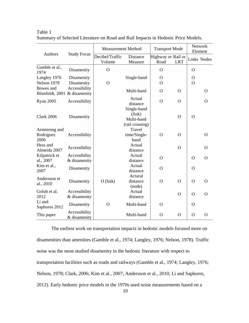
Table 1

Summary of Selected Literature on Road and Rail Impacts in Hedonic Price Models.

Authors Study Focus

Measurement Method Transport Mode Network

Element

Decibel/Traffic

Volume

Distance

Measure

Highway or

Road

Rail or

LRT Links Nodes

Gamble et al.,

1974 Disamenity O O O

Langley 1976 Disamenity Single-band O O

Nelson 1978 Disamenity O O O

Bowes and

Ihlanfeldt, 2001

Accessibility

& disamenity Multi-band O O O

Ryan 2005 Accessibility Actual

distance O O O

Clark 2006 Disamenity

Single-band

(link)

Multi-band

(rail crossing)

O O

Armstrong and

Rodriguez

2006

Accessibility

Travel

time/Single-

band

O O O

Hess and

Almeida 2007 Accessibility

Actual

distance O O

Kilpatrick et

al., 2007

Accessibility

& disamenity

Actual

distance O O O

Kim et al.,

2007 Disamenity

Actual

distance O O

Andersson et

al., 2010 Disamenity O (link)

Actural

distance

(node)

O O O O

Golub et al.

2012

Accessibility

& disamenity

Actual

distance O O O

Li and

Saphores 2012 Disamenity O Multi-band O O

This paper Accessibility

& disamenity Multi-band O O O O

The earliest work on transportation impacts in hedonic models focused more on

disamenities than amenities (Gamble et al., 1974; Langley, 1976; Nelson, 1978). Traffic

noise was the most studied disamenity in the hedonic literature with respect to

transportation facilities such as roads and railways (Gamble et al., 1974; Langley, 1976;

Nelson, 1978; Clark, 2006; Kim et al., 2007; Andersson et al., 2010; Li and Saphores,

2012). Early hedonic price models in the 1970s used noise measurements based on a

11

fixed distance (usually 1,000 feet or less) from highways. Models using cross-sectional or

time-series data generally concurred that residential property values are negatively

affected by the level of noise (Nelson, 1982).

Actual noise levels, however, are quite expensive to measure at the parcel level,

which led to the use of distance as a fairly good proxy for field measurement of actual

noise levels (Bailey, 1977). While many studies considered a single fixed distance area

(e.g., within 1000 ft. or a quarter mile) considered to be an impact zone of noise pollution

(Langley 1976; Kim et al., 2007), some studies used dummy variables for multiple

distance bands (Bowes and Ihlanfeldt, 2001; Clark, 2006; Li and Saphores, 2012).

Multiple distance bands allow hedonic models to capture non-linear relationships

between price impacts and distance from a transportation facility that may result from

distance decay and/or the net effects of accessibility and disamenities (De Vany, 1976).

For instance, Golub et al. (2012) showed that while proximity to LRT stations generally

has a positive effect on property values that decays with distance from the station,

extremely close proximity (i.e., within 200 ft.) is penalized by the market for single-

family home values (Golub et al., 2012). This type of “donut” effect for residential

property values is something we investigate further in the present paper.

More recently, thanks to the growing use of geospatial data, geographic

information systems (GIS) and spatial analysis techniques, researchers have been able to

calculate actual distance to highways from each parcel to use as an explanatory variable

(Geoghegan et al., 1997; Hess and Almeida, 2007). Researchers have tested which of

several distance metrics has the closest statistical relationship with property values

(Thériault et al., 1999). Hess and Almeida (2007) found that a network distance model

12

returned more significant parameter estimates, while a Euclidean distance model returned

higher but more uncertain parameter estimates. Both of their models concluded that

accessibility has a positive effect on residential property values in general, and the value

of property located in the study area decreases by $2.31 per foot of Euclidian distance

from a light rail station, compared with $0.99 per foot of network distance.

Since noise is a function of both distance and traffic volume, Li and Saphores

(2012) used distance buffers interacting with different traffic count metrics. Their study

of residential property values in Southern California not only confirmed that the negative

impact on sales prices was larger for the 100-200m band than the 200-400m band, but

also that sale prices were more sensitive to truck flow volume specifically than to overall

traffic volume (Li and Saphores, 2012).

Accessibility effects on residential property values for highway exits and railway

stations have also been studied. Many researchers, however, used actual distance or travel

time measurements from the highway exits and railway stations to investigate the price

effect by each measurement unit (Ryan, 2005; Armstrong and Rodriguez 2006; Hess and

Almeida, 2007), which can restrict the relationships between price impacts and distance

from highway exits or railway stations. In addition, studies mentioned above did not take

into account traffic noise, air pollution, or crime rate as disamenity factors that might negatively

influence property values near highway exits and/or railway stations.

While many researchers have modeled the price effects of a single type of

transportation infrastructure on either proximity or disamenity, relatively few have

considered the effects of multiple transportation modes such as rail and road

simultaneously. Ryan (2005) found that accessibility to highways plays a more important

13

role than accessibility to LRT for non-residential property values. Andersson et al. (2010)

found that road noise impacts on property values are larger than railway noise impacts.

These two studies partially support our theoretical framework in the next section, in that

both accessibility and noise impacts are larger for road than for railway, though Ryan

(2005) studied non-residential property and neither study used distance bands to test the

non-linearity of the relationships.

A factor that has not received enough attention to date is whether the effects of

proximity vary depending on whether distance is measured from the nodes (i.e., exits or

stations) or the links of the network. Many studies have investigated one or the other, but

few have tried to disentangle the price effects of nodes vs. links. Of the papers reviewed,

only Golub et al. (2012) distinguished between distance from the nodes and the links for

rail, while Kilpatrick et al. (2007) did so for highways. Anderssson et al. (2010)

conducted perhaps the most comprehensive analysis: they used actual distance from the

nodes for rail and highway but decibels for noise measure of the links for rail and

highway.

Although not shown in Table 1, some studies have investigated whether the noise

discount may be affected by highway configurations such as tunnels, noise barriers, over-

or underpasses, and sound berms. A study in Montreal, Canada showed that construction

of noise barriers generated a small negative effect in the short run (6% decrease in sale

prices) but generated a relatively large negative effect in the long run (11% decrease)

(Julien and Lanoie, 2008). Another study in South Korea showed that residential property

values are negatively associated with highway overpasses (Kim et al., 2007).

14

The final paper reviewed here is excluded from Table 1 because it dealt with

airports rather than rail or highway. Nevertheless, De Vany (1976) provides an important

theoretical foundation for our work because it hypothesized an idealized relationship of

price with distance that separates out a positive accessibility premium and a negative

noise discount, each of which decays at a different rate with increasing distance from the

airport. The two curves are added to form a hypothetical net effects, inverted U-shaped,

curve. De Vany (1976) then developed an empirical model with multiple distance bands

around Love Field airport in Dallas, Texas and plotted their coefficients against distance,

which proved consistent with his proposed theoretical framework. Specifically, he found

that the negative noise externalities were larger than the accessibility effect within one

mile, while the net effect was positive for the 2-3 mile band.

In this study, we build on De Vany’s (1976) theoretical and empirical approach

to studying airports, and adapt it to modeling the net accessibility and disamenity effects

of rail and highway. As Table 1 shows, our study will differ from previous work on

highway and rail by combining the effects of links and nodes for both highways and LRT

using multiple distance bands. Our approach also controls for whether the highways are

above, at, or below grade, in addition to other more commonly used structural and

neighborhood control variables as well as proximity to several categories of open space

amenities.

Theoretical Model

In this section, we expand De Vany’s theoretical net effects model for airports

into a 2x2 schematic diagram for the effects of the nodes and links of rail and highway

networks. In doing so, one must consider the difference between accessibility and

15

disamenities such as noise and air pollution, the difference in how their effects decay

with distance from nodes and links, and the difference between highway and rail. The

following observations guided the development of the theoretical model.

First, accessibility accrues only to the nodes because travelers cannot access

limited-access freeways and light-rail trains except at exits and stations respectively.

Thus, if the effects of nodes and links are treated separately, the positive externalities of

accessibility should be maximized at the nodes themselves and decay from there.

Second, disamenity, primarily noise, should emanate from both nodes and links

and decay with increasing distance (Nelson, 1982). Other particular disamenities can

depress housing values to varying extents, such as crime or traffic around rail stations

(Bowes and Ihlanfeldt, 2001), or air pollution around highways (Bae et al., 2007).

Third, nodes should generate net benefits resulting from the sum of the positive

and negative impacts at each distance from the exit or station. Links, on the other hand,

logically should generate only negative disamenities.

Fourth, the negative disamenities diffusing from the nodes and links should

theoretically decay more steeply with distance than the positive benefits of accessibility.

We hypothesize this first because noise falls off rapidly and the health effects of air

pollution are not well understood by the general public and the perception of it can be

subjective and inconsistent (Nelson, 1982). Second, accessibility benefits extend farther

geographically due to extended access provided by motor vehicles.

Fifth, rail stations should generate a steeper decay of accessibility and earlier

leveling off to negligible levels because access modes include slower forms of

transportation such as walking, bicycling, or bus. Highway exits should generate a more

16

gradual decay and extended range because access is almost exclusively by private

automobile.

Sixth, highway links and nodes should generate higher levels of disamenity

because the traffic noise and pollution is constant, and the spatial extent of that

disamenity should reach to farther distance bands. Rail links and nodes may generate

lower levels of disamenity because the traffic and noise are intermittent, although

perceptions of crime and/or loud voices and train horns from the station area could alter

this hypothesis.

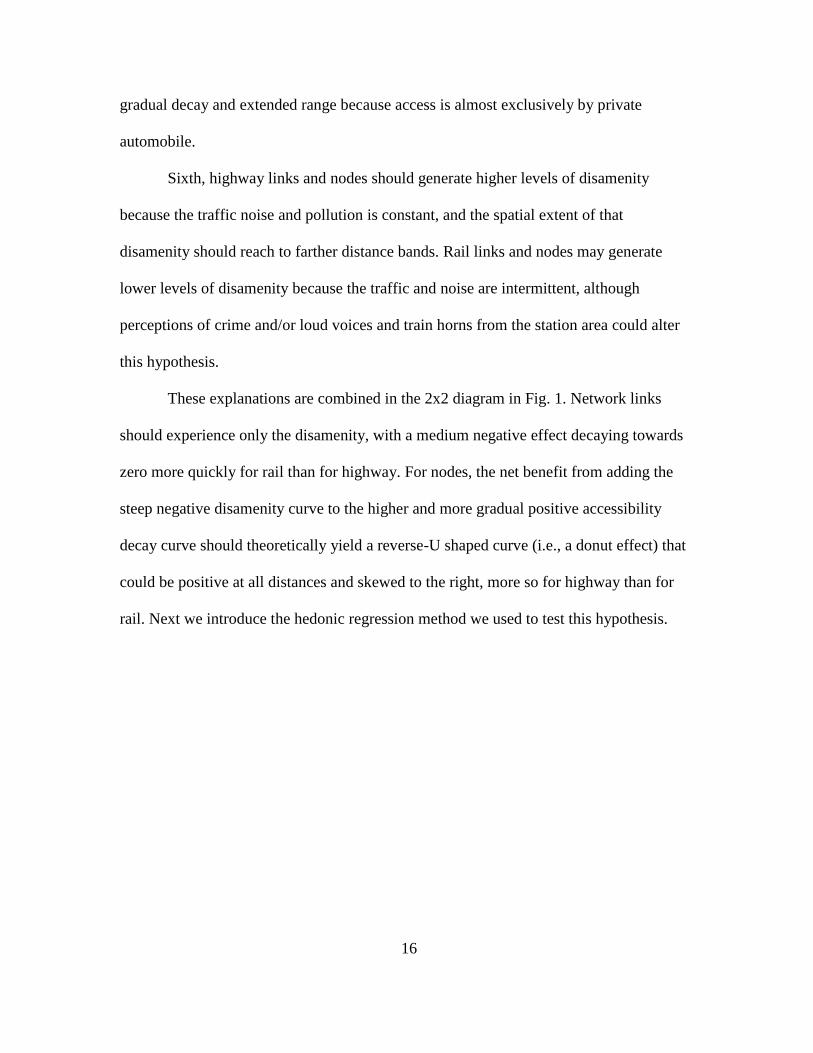
These explanations are combined in the 2x2 diagram in Fig. 1. Network links

should experience only the disamenity, with a medium negative effect decaying towards

zero more quickly for rail than for highway. For nodes, the net benefit from adding the

steep negative disamenity curve to the higher and more gradual positive accessibility

decay curve should theoretically yield a reverse-U shaped curve (i.e., a donut effect) that

could be positive at all distances and skewed to the right, more so for highway than for

rail. Next we introduce the hedonic regression method we used to test this hypothesis.

17

Fig. 1. Conceptual Framework for Net Benefit of Combined Impacts of Accessibility and

Disamenity

Methods

The term “hedonic modeling” was coined by Court in 1939 and popularized by

researchers such as Griliches (1961) and Rosen (1974)—see Goodman (1998). Hedonic

modeling is designed to estimate the implicit value of differences in property

characteristics, which includes amenities and disamenities. Thus, hedonic modeling is

well suited to estimating the market value of externalized costs such as noise or pollution,

or externalized benefits such as access to freeways or light rail. Empirical hedonic models

using house sales prices as the dependent variable are widely accepted because housing is

a commonly traded and commonly understood good that has a specific set of

characteristics (Champ et al., 2003; Morancho, 2003). Housing prices can be determined

18

by internal and external characteristics such as structural characteristics (e.g., lot size,

interior square footage, number of rooms, number of stories, age, presence of a garage or

pool), neighborhood characteristics (e.g., proximity to central business district, highways,

and bodies of water), and environmental characteristics (e.g., urban open spaces and

amount of greenness nearby).

Nonlinear relationships are common in hedonic pricing models. Housing prices

are known to increase at a decreasing rate with lot size and interior square footage, for

instance (Champ et al 2003). Neighborhood characteristics may also be non-linear

because of distance decay (Andersson et al 2010). In this paper, we tested linear, semi-

log, and translog (ln-ln) functional forms (Malpezzi, 2003). The translog model was

selected based on comparing the linearity of scatterplots for the transformed variables and

the results of adjusted R-squared, Akaike Information Criterion (AIC), and Bayesian

Information Criterion (BIC). In addition, heteroskedasticity was evaluated using the

Koenker-Bassett test (Kim et al., 2003; Drukker et al., 2013).

Spatial effects, in the form of spatial dependence, spatial heterogeneity, or both,

are another common issue with hedonic real estate models. Spatial dependence or spatial

autocorrelation implies spatial correlation among observations in cross-sectional data that

are assumed to be independent, while spatial heterogeneity implies spatial correlation of

the error terms (Anselin, 1988). To obtain unbiased, consistent, and efficient estimates,

spatial dependences and heteroskedasticity should be tested and addressed with proper

methods if either one or both spatial effects exist (Anselin, 1988; Kim et al., 2003).

Moran's I statistics and Lagrange multiplier tests were used to test for presence of spatial

effects (Champ et al., 2003).

19

A number of approaches have been developed to deal with spatial effects. One

widely used approach is to add spatial fixed-effects dummy variables (e.g., zip code

zones, school districts, or census block groups) in a hedonic regression model to

represent neighborhood effects or housing submarkets (Kuminoff et al, 2010). A more

recently developed alternative, which we take in this paper, is the spatial econometric

approach (Anselin, 1988; Anselin and Florax, 1995; Anselin and Bera, 1998). The spatial

econometric approach directly incorporates data about the contiguity of observations and

does not require any preconceived assumptions about which fixed-effects zonation

system best matches housing submarkets (Anselin and Arribas-Bel, 2013, p. 7).

Given that test results confirm the presence of both spatial dependences and

heteroskedasticity in our dataset (see Results, below), we, thus, applied combined spatial

lag and spatial error model using the generalized spatial two-stage least squares

(GS2SLS) estimator with the heteroskedasticity option using GeoDaSpace software

(Arraiz et al., 2010; Drukker et al., 2013). Queen contiguity was used to generate the

spatial weights matrix. Equation (1) and (2) provide the general form of combined spatial

lag and error model used in this paper:

(1)

(2)

where is a vector of house sales prices; is the constant term; is the coefficient of the

spatial autocorrelation; W is the standardized spatial weights m×m matrix with zero

diagonal terms that assigns the potential spatial correlation; the product is the

spatially lagged dependent variable; X is the m×n matrix of explanatory variables; is

the n×1 vector of the coefficients of the explanatory variables; is the n×1 vector of

20

spatial autoregressive error term; is the coefficient of the spatially correlated error term;

is the spatially lagged error terms; and is independent but heteroskedastically

distributed error. Thus, if there are no spatial effects in the dependent variable, the

coefficients of the spatially correlated lag and error (i.e., and ) become zero, and then

both equations (1) and (2) reduce to a standard OLS model.

In this paper, we estimate and report results for the combined spatial lag and error

model using the GS2SLS estimator with positive and significant and . We also

distinguish between direct and indirect effects in interpreting the coefficients, as

recommended for models that use a spatial lag term (Kim et al., 2003; Fischer and Wang,

2011).

Study Area and Data

The study area is the City of Phoenix, Arizona, located in the Sonoran Desert in

the southwestern US and incorporated as a city in 1881. It is the capital and largest city

(517 square miles) in the State of Arizona. It is the sixth most populous city (1.4 million),

situated in the 14th

largest Metropolitan Statistical Area (4.2 million) in the US. Because

much of its growth occurred in the mid to late 20th

century, it features a moderately dense

urban land-use structure well connected by arterials and freeways, which lowers the

public transportation mode share compared to other US cities of a similar size.

Transportation mode shares to work for the Phoenix MSA are 89.1% by motor vehicles

(solo driver and carpool), 0.7% by bicycle, 2.3% by public transit (half of the rate for the

US overall), 6.3% by non-motorized modes, and 1.6% by other (Kuby and Golub, 2009,

p. 37). Phoenix is a prototypical example of cities largely built up in automobile era; if

21

this research shows significant price effects of proximity to light rail, a stronger case can

be made for investing in public transit in similar cities.

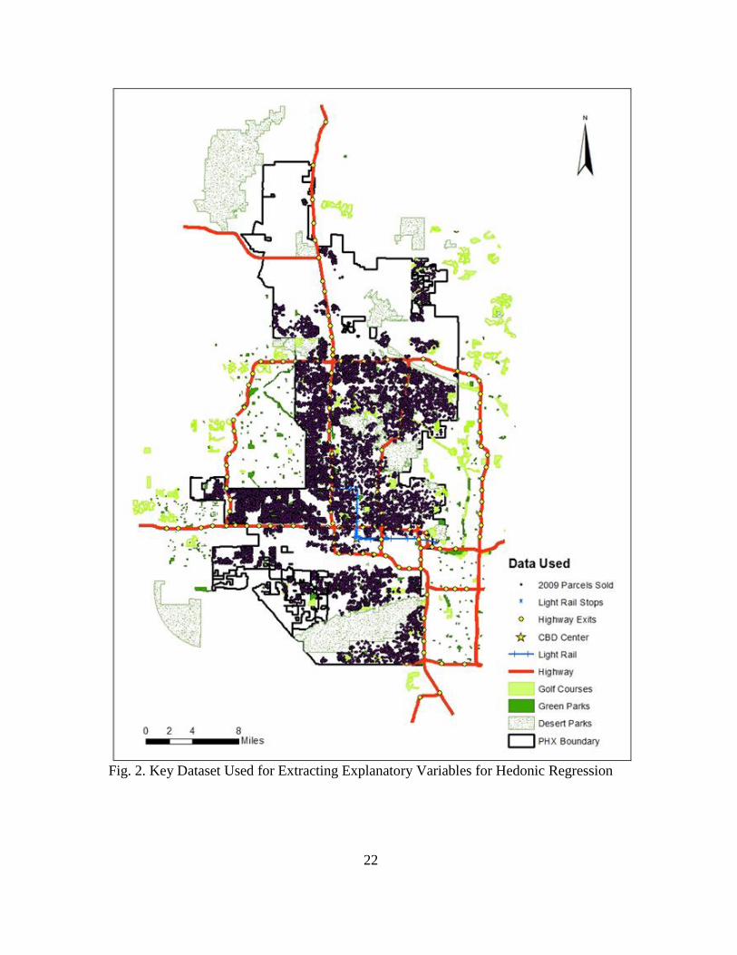
Data for this study were gathered from various sources (Fig. 2). The dependent

variable is the sales price of single-family detached homes in 2009 obtained from the

Maricopa County Assessor's Office (MCAO). The Assessor’s dataset included various

attributes of each house that were incorporated as structural explanatory variables, such

as lot size, interior living space, number of bathroom fixtures (bathtubs, toilets, etc.),

presence of a swimming pool, and construction year. Other attributes in the Assessor’s

dataset such as number of rooms, number of stories, size of patio, size of garage, and date

of sale were not included in the model because of missing information and

multicollinearity.

For the spatial regression models, we created a spatial weights matrix using

Thiessen polygons based on the centroids of all parcels sold in 2009. We also added a

monthly home price index variable to control for the volatile housing market of 2009.

Despite the volatility, we focus on 2009 because it is the first full year of light rail

operation, which opened in December 2008.

22

Fig. 2. Key Dataset Used for Extracting Explanatory Variables for Hedonic Regression

23

For neighborhood characteristics of a home, tract-level median household income

and population density were collected from the 2010 U.S. Census. Neighborhood

amenities such as green urban parks, desert parks, and golf courses were collected from

available GIS data sources and used to create a proximity measure to each. We measured

the distance between downtown Phoenix and each residential property from the

intersection of Central Avenue and Washington Street, representing the central point of

the Central Business District (CBD). Distance from highways was measured in three

bands up to 350m (about .21 miles). Distances from highway exits to parcels were

measured in 400m bands, up to 3200m (about 1.92 miles). Distances from the LRT

stations to individual parcels were measured in 300m bands out to 3000m (about 1.8

miles), and distances from the LRT track were measured in 100m bands, out to 300m (.18

miles). All distances were measured in Euclidean terms.

For the environmental characteristics, we used land-cover classification data

produced by the Central Arizona-Phoenix Long-Term Ecological Research (CAP-LTER)

project based on 2005 and 2009 high-resolution QuickBird imageries (Fig. 3). The

percentage of land area covered by trees or grass within a 200m buffer around each

individual property sold were extracted to estimate neighborhood greenery. In addition,

the highway configurations (below grade, elevated, or at grade) were manually analyzed

using the Google Earth street view and assigned as dummy variables to each home

according to the characteristic of the nearest highway link.

24

Fig. 3. Phoenix Land Cover Classification Map Using Quickbird Imageries (Source:

Central Arizona-Phoenix Long-Term Ecological Research (CAP LTER), National

Science Foundation Grant No. BCS-1026865).

25

There were 24,155 single-family home sales in 2009 in the County Assessor’s

database. Of these, 4,006 observations were dropped due to missing data, improper

attribute values, and outliers such as lot sizes much larger than usual (e.g., lot size over

50,000 sq ft or sale price over $2 million), leaving 20,149 observations. APPENDIX A

describes the summary statistics of the variables.

Results

Multiple regression analysis was initially conducted using SPSS Statistics 20 for

Windows. A best fit was found using a translog form, likely due to the non-linear

relationships between many of the independent variables and sales prices. The resulting

model fit is quite strong with an adjusted R2 of 0.766. As noted in the Methods section,

however, presence of spatial dependence and spatial heterogeneity was confirmed by the

robust Lagrange multiplier test value of 272.27 (p=.000) for lag, 1498.32 (p=.000) for

error, and a Koenker-Bassett test value of 1,607.97 (p=.000) for heteroskedasticity. To

take spatial effects into consideration, we applied a combined spatial lag and spatial error

model using GeoDaSpace to estimate the coefficients of the explanatory variables.

26

Table 2

Estimation Results.

Variable Coef Std. Err. z-stat Sig.

(Constant) 1.4248 0.204 6.99 0.000

Structural Variables ( )

Sqm (ln) 0.6276 0.0163 38.56 0.000

Area_sqm (ln) 0.1726 0.0099 17.44 0.000

Bathfix 0.0381 0.0023 16.41 0.000

Age -0.0060 0.0003 -21.96 0.000

Pool 0.0815 0.0063 12.87 0.000

Neighborhood Variables ( )

N_GPark (ln) 0.0012 0.0039 0.31 0.759

N_DPark (ln) -0.1491 0.0039 -38.36 0.000

N_Golf (ln) -0.0342 0.0033 -10.37 0.000

N_CBD (ln) 0.0794 0.0114 6.98 0.000

Hway_150m -0.0271 0.0265 -1.02 0.306

Hway_250m 0.0013 0.0242 0.05 0.959

Hway_350m -0.0204 0.0228 -0.90 0.369

LT_100m -0.0246 0.1480 -0.17 0.868

LT_200m -0.0155 0.1080 -0.14 0.886

LT_300m -0.1202 0.0850 -1.41 0.157

Exit_400m 0.1455 0.0300 4.85 0.000

Exit_800m 0.0980 0.0132 7.45 0.000

Exit_1200m 0.1161 0.0106 10.95 0.000

Exit_1600m 0.1097 0.0114 9.66 0.000

Exit_2000m 0.1064 0.0121 8.79 0.000

Exit_2400m 0.0528 0.0118 4.48 0.000

Exit_2800m 0.0859 0.0122 7.05 0.000

Exit_3200m 0.0705 0.0125 5.64 0.000

S_300m 0.8835 0.1225 7.21 0.000

S_600m 0.6597 0.0693 9.52 0.000

S_900m 0.5477 0.0506 10.82 0.000

S_1200m 0.4296 0.0446 9.63 0.000

S_1500m 0.4089 0.0440 9.30 0.000

S_1800m 0.2398 0.0497 4.82 0.000

S_2100m 0.2435 0.0326 7.46 0.000

S_2400m 0.1885 0.0323 5.83 0.000

S_2700m 0.1647 0.0301 5.47 0.000

S_3000m 0.1010 0.0250 4.04 0.000

M_income (ln) 0.4102 0.0159 25.88 0.000

Pop_dens (ln) -0.0275 0.0061 -4.53 0.000

Environmental Variables ( )

P_trees 2.3515 0.0607 38.75 0.000

P_grass 0.4088 0.0432 9.47 0.000

Above 0.0010 0.0541 0.02 0.986

Below 0.1695 0.0332 5.11 0.000

H_Index -0.0006 0.0003 -1.97 0.049

Rho 0.1297 0.0089 14.65 0.000

Lambda 0.3915 0.0115 33.94 0.000

Pseudo R² 0.782

Spatial Pseudo R² 0.769

27

Table 2 shows the coefficients, significance levels, and Pseudo R2 for the spatial

lag and error model. While the Pseudo R2 (.782) cannot be interpreted exactly as one

would interpret an OLS R2, a higher Pseudo R

2 still can be interpreted as better model fit

than a lower one (Anselin, 1988). The spatial hedonic regression results partially validate

our theoretical model of the accessibility and amenity impacts of highway and LRT

nodes on the residential property values, but are not validated for the highway and LRT

links.

Overall, most of the independent “control” variables are highly significant at the

0.001 level except distance to nearest green parks, and highways above grade. All of the

coefficients for the structural variables have the expected signs. Measures of living area,

lot size, number of bathroom fixtures, and presence of a pool are positively related to

housing prices, while the age of the house is negatively related. For instance, marginal

willingness to pay (MWTP) for one m² increment of living area is $596, which includes

indirect effect of $77 captured through a spatial multiplier (i.e., ), while

MWTP for a year increment of house age is -$857, which also includes indirect effect of

-$111. The signs of the socioeconomic and neighborhood coefficients are as expected,

with a few exceptions. The coefficient of median household income is positive as

expected, and that for population density is negative as expected, and both are significant

at the 0.001 level. The effect of proximity to green parks is not significant. This is

somewhat corroborated by the literature, which has shown mixed results, both positive

and negative, for the price effects of proximity to green parks (e.g., Tyrväinen, 1997;

Shultz and King, 2001). Neighborhood characteristics such as proximity to nearest large

desert preserve and golf courses have a positive effect on the property values, while

28

distance from the CBD has a negative effect. The amount of green space with trees and

grass in the neighborhood positively affect property values as expected. The land fraction

covered with trees is more valuable than for grass, which makes sense considering the

shade and cooling benefits of trees compared with grass. Thus, MWTP for one percent

increment of tree coverage is $3,364, which includes indirect effects of $436 because of

the spatially weighted average of housing prices in a neighborhood, while MWTP for one

percent increment of grass coverage is $585 including indirect effects of $76.

Finally we turn to the transportation infrastructure variables of greatest interest in

this study. Our hypotheses concerning the disamenity of proximity to highway and light

rail links are not validated in this study. The results indicate that while five of the six

coefficients on the dummy variables for the distance bands from highways (up to 350m)

and light-rail (up to 300m) have negative signs as hypothesized, none are even close to

being significant, even at the 0.1 level. Thus, disamenities such as noise, represented by

distance from both highway and light rail track, appear to have no significant effect on

residential property values.

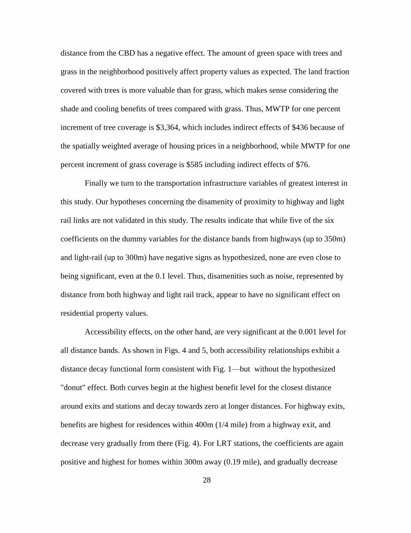
Accessibility effects, on the other hand, are very significant at the 0.001 level for

all distance bands. As shown in Figs. 4 and 5, both accessibility relationships exhibit a

distance decay functional form consistent with Fig. 1—but without the hypothesized

"donut" effect. Both curves begin at the highest benefit level for the closest distance

around exits and stations and decay towards zero at longer distances. For highway exits,

benefits are highest for residences within 400m (1/4 mile) from a highway exit, and

decrease very gradually from there (Fig. 4). For LRT stations, the coefficients are again

positive and highest for homes within 300m away (0.19 mile), and gradually decrease

29

from there (Fig. 5). Contrary to our hypotheses, the “donut” effects based on nuisance

effects at short distances around the highway exits and rail stations are not evident in

either graph. Thus, MWTP for a median priced home in the 400m band of highway exit is

$22,405, which includes indirect effects of $2,906 because of the spatially weighted

average of housing prices in a neighborhood, while MWTP for one in the 300m band of

LRT station is $203,055 including indirect effects of $26,336.

Fig. 4. Coefficients of Distance from the Highway Exit

30

Fig. 5. Coefficients of Distance from the Light Rail Station

The results partially validate our hypotheses that higher-speed vehicles (cars)

travel longer distance in a short period of time and thus dramatically extend the range of

accessibility benefits. However, in addition to the greater extent of the highway

accessibility effect, the absolute size of the coefficients for highway is lower than for rail

across the impact range. We speculate that this may be due to Phoenix’s extensive

highway network that shares the impacts across the city, whereas only a small portion of

the city shares the light rail benefit. On the other hand, it makes intuitive sense and

validates our hypothesis that the benefit of LRT stations decline steeper than that of

highway because residents access LRT stations via numerous modes, including slower

ones such as walking, biking, or bus. However, it is surprising that the geographical range

of impacts of LRT station reaches up to 3000m.

31

Although we do not have clear evidence why there are no disamenity impacts for

both highway and light rail links, there are a couple of possible explanations. First,

properties adjacent to highway links are protected by sound walls, which reduces noise

disamenity, and possibly reduces some air-pollution as well. Second, the data used for

measuring distance from highway links is a road centerline feature, which creates

inaccurate distance bands because highway link has non-negligible width. Third, noise

nuisance of light rail may not exceed noise generated by traffic on the same road because

light rail tracks are built mostly in the middle of road way and light rail operates less

frequently than cars do. Fourth, light rail is operated by electricity, so it does not emit

polluted air.

The lack of evidence for a donut effect around nodes may be explained in similar

ways. Noise and air-pollution may be reduced by sound barriers near highway exits and

point feature class used for measuring distance bands for the exits does not create

accurate distance variables. Moreover, noise nuisance and air pollution near light rail

stations may be too small to capture for the same reasons with the light rail link.

Lastly, the regression result of the variable representing the highways situated

below grade is statistically significant at the level of 0.001 with a positive coefficient as

expected, presumably due to their reduced noise levels and visibility. The estimated

coefficient of the elevated highways, however, is not significant.

Conclusions

The purpose of this study was to measure the net effects of the nodes and links of

road and rail infrastructure on single-family home values using spatial hedonic regression

techniques with distance bands. Previous studies have developed separate models of

32

some subset of these relationships, such as between housing prices and highway noise

(Gamble et al., 1974; Langley, 1976), noise of both road and rail (Andersson, 2010), rail

accessibility (Cervero, 1996; Hess and Almeida, 2007; Golub et al., 2012), or

accessibility of both highway and light rail (Ryan, 2005). To our knowledge, however, no

hedonic pricing study of the effect of highway and LRT on house prices has attempted to

disentangle the positive and negative distance-decay effects of proximity to the

infrastructure of light rail and highway nodes and links simultaneously. We hypothesized

that the accessibility benefits of light rail and highway accrue to the LRT stations and

highway exits (i.e., the network nodes) specifically, while the disamenities of noise and

pollution should emanate from the rail and highway links as well as the nodes. Using

distance buffers, we have tested the significance of the distance from the nodes and links

and plotted the coefficients as a function of the distance from the infrastructure to

estimate the distance decay of net amenities and disamenities. Numerous other

independent variables were included to control for structural characteristics of the house

and of the neighborhoods, including several measures of green space and distance from

different kinds of parks. In addition, a monthly home sales price index was added to

control for the volatility of the housing market over the course of 2009 immediately

following the opening of the Valley Metro LRT, and a spatial regression model was used

to test and control for spatial effects.

The main results of the study show that distances from both kinds of transport

nodes (LRT stations and highway exits) show a typical exponential decay curve

consistent with the theorized model for benefit. Unexpectedly, however, they are not

consistent with our hypothesis of a negative disamenity effect in the immediate vicinity

33

of stations and exits. The greater range of highway accessibility benefits is also consistent

with our hypothesis based on the faster speed of travel to and from highway exits using

motor vehicles compared with the slower speed of some of the modes of transport used to

access LRT stations. However, magnitude of accessibility benefit of LRT stations is

much larger than that of highway exits, contrary to our hypothesis. The effects of

proximity to the road and rail links were not significant. Below-grade highways had a

relatively positive impact on nearby houses compared with highways at ground level or

above.

Further research is required to investigate why proximity to the nodes and links—

which theoretically should have a primarily negative disamenity from noise and air

pollution—was not statistically significant for both highway and rail. One possible

explanation is that local highway authorities have properly installed sound walls or sound

berms along the highway adjoining residential areas and applied noise dampening

pavements to reduce noise impact, and the relevant laws such as the US Noise Control

Act work well in Phoenix, Arizona1. Another possible explanation is that the number of

properties located very close to exits or rail stations is very small and this may bias the

statistical relationship between distance bands one way or the other.

Results for the highway links might be improved with more accurate data. For

instance, highways have non-negligible width, and some have more lanes than others.

Using the centerlines of highways is not an exact measure of the distance from houses to

the edge of the highway. Representing highways as polygons rather than lines might

1 Almost all residential houses adjacent to the highway in Phoenix are protected by noise barriers or sound

berms.

34

produce more accurate and significant results. We leave the further investigation of these

and other explanations to future research.

Finally, this paper focused on single-family detached housing values. It would be

useful to apply the multi-band, node-link approach developed here to multi-family

housing and commercial real estate, as this would provide useful information to

developers, planners, and policy-makers concerned with infill and transit-oriented

development.

35

CHAPTER 3

IMPACTS OF HIGHWAYS AND LIGHT RAIL TRANSIT ON COMMERCIAL

PROPERTY VALUES

Abstract

This study investigates the impacts of positive and negative externalities of highways and

light rail on commercial property values in Phoenix, Arizona. We hypothesize that the

positive externality (i.e., accessibility) of highway and light rail accrues at exits and

stations, whereas nodes and links of highways and light rail emanate negative effects.

Positive and negative effects decay with increasing distance and are captured by multiple

distance bands. Hypotheses are tested using a spatial error regression model. Results

show that accessibility benefits of transport nodes are positively and significantly

associated with all commercial property values. The distance-band coefficients form a

typical distance decay curve for both modes with no detectable donut effect immediately

around the nodes. Unexpectedly, impacts of light rail stations extend farther than those of

highway exits. As hypothesized, the links of highway and light rail are negatively

associated with property values. When the sample is subdivided by type of commercial

property, the magnitude and extent of impacts of distance are surprisingly consistent,

with light rail stations having more positive impact than highway exits on all three classes

of commercial property: industrial, office, and retail and service. Rail links have a

significant negative impact on price for all three types of commercial property, but

highways have a significant negative impact only on industrial and retail/service

properties.

Keywords: highway, light rail, spatial error model, node, link, commercial property value

36

Introduction

Numerous studies have focused on transportation facilities as an important

determinant of property values because they provide accessibility as well as nuisance

effects that may alter property values (Vessali 1996; Bateman et al, 2001). While a

considerable body of hedonic literature has investigated residential property values, fewer

studies have addressed non-residential or commercial property values (Weinberger 2001;

Ryan 2005). Of these, even fewer have considered the impacts of multiple modes of

transportation, such as rail and highway, and fewer still have attempted to disentangle the

separate effects of transportation nodes and links in their models so that they can capture

the distance decay of positive and negative impacts. Seo et al. (2014) built a hedonic

price model with this comprehensive set of factors (i.e., distance decay around the nodes

and links of highways and light rail transit) for residential property values in Phoenix,

Arizona. This study extends that work to an analysis of commercial property.

The purpose of this study is to use the theoretical framework of Seo et al. (2014)

to estimate the net impacts of network nodes and links of rail and road facilities on

commercial property values in Phoenix, AZ. This study may help locating commercial

property to maximize accessibility and profit based on the distance from transport nodes.

This study may also inform policy makers on designing tax-increment financing2

mechanisms for funding new public transportation investments (Anderson 1990; Medda

2012). We utilize hedonic regression models to estimate the impacts at various distances

of nodes and links of highways and light rail networks on commercial property values.

We also subdivide commercial properties into office, industrial, and retail and service

2 Tax increment financing (TIF) is a special funding tool used as a subsidy for infrastructure and

community-improvement projects such as redevelopment in urban core and new road construction.

37

categories to test whether transportation facilities have dissimilar effects on the sale

prices of different types of commercial property. Hence, the specific research questions

are:

How do commercial property markets (i.e., as a whole and by type) value the

positive and negative effects of proximity to highway compared with light rail

facilities?

How do commercial property markets value amenities and disamenities of

proximity to transport nodes compared with transport links?

How do these positive and negative effects decay (or increase) with distance to

transportation infrastructure?

How do such effects vary by type of commercial property?

We compare the results of our model with Seo et al.’s results for residential

property values in the same city and time period.

Literature Review

As noted earlier, the literature on hedonic studies of transportation infrastructure

impacts on residential property values is quite extensive. In contrast, a relatively smaller

body of literature exists on the determinants of commercial property values, and only a

handful of studies focused on the transportation-related factors (Weinberger 2001; Ryan

2005; Billings 2011; Golub et al., 2012). Many studies focused mainly on the impacts of

access to the central business district (CBD), but some of these studies also included

transportation-related factors as explanatory variables (Clapp 1980; Brennan et al., 1984;

Sivitanidou 1995; Sivitanidou 1996; Dunse and Jones 1998). APPENDIX B summarizes

38

selected hedonic studies of commercial property values with regard to the transportation-

related factors they considered:

dependent variables (type of commercial property)

amenity (accessibility) and disamenity (noise, traffic, air pollution, crime) or both

distance decay of these effects;

mode(s) of transport studied;

whether distance effects are measured from the nodes or links of the network.

time frame (single- or multi-year)

Dependent variables used for the studies on commercial property vary based on

availability (i.e., sales transaction data, actual transacted rents or effective rents, asking

rents, and assessed property or land values). Although actual transacted sales prices are

preferred (Ihlanfeldt and Martinez-Vazquez 1986) because they capture the real property

market behaviors, commercial property sales prices or effective rents are hard to obtain

because these data are often not open to public use (Mills 1992; Wheaton and Torto

1994; Landis and Loutzenheiser 1995; Bollinger et al., 1998).The majority of studies

utilized asking rents as the dependent variable, which were usually provided by large

commercial real-estate consulting or brokerage firms such as CoreLogic, Coldwell

Banker, and TRI Commercial Real Estate Services for academic research (Mills 1992;

Landis and Loutzenheiser 1995; Bollinger et al., 1998; Ryan 2005). The use of asking

rents is supported by Glascock et al. (1990), who found an extremely close relationship

between effective rents and asking rents. However, both actual transacted rents and

asking rents from the databases of commercial real estate service firms may yield biased

39

samples. For instance, some databases of commercial real estate firms are limited to a

specific size of office spaces (Landis and Loutzenheiser 1995). Moreover, sometimes the

number of cases was too small for estimating a model (Dunes and Jones 1998; Nelson

1982). Brennan et al. (1984) used actual transacted office rents as a dependent variable

with only 29 cases. As an alternative, Sivitanidou (1996) and Cervero and Duncan (2002)

used assessed property values as the dependent variable.

The use of assessed or estimated property values has an advantage over the use of

actual sales prices, effective rents, and asking rents. The assessed property values are not

a sample but rather the whole population, meaning that sampling error is greatly reduced

(Champ et al., 2003). Sivitanidou (1996) found a correlation between sales prices and

assessed values on office-commercial firms of 0.98 for office-commercial firms, which

led her to use assessed values in order to cope with spatial collinearity issues with a larger

number of cases. Transit-related hedonic research by Cervero and Duncan (2002) used

estimated land values, which were apportioned from total taxable property values

including improvements by the county assessor's office. They argued that there is no

evidence that estimated land values are biased in a certain direction. However, despite

these advantages, the use of assessed property value as the dependent variable is still

problematic, because the way some assessor offices estimate property values can be

similar to hedonic regression (Arizona Department of Revenue 2009), making circular

reasoning a concern.

In addition, most studies have considered only one type of commercial property,

such as office property (Landis and Loutzenheiser 1995; Dunse and Jones 1998),

industrial property (Sivitanidou and Sivitanides 1995), or retail property (Damm et al,

40

1980). In contrast, Ryan (2005) studied two types of commercial properties (i.e., office

and industrial properties), while others have analyzed commercial property as a whole

(Cervero and Duncan 2002; Golub et al, 2012). Effects may differ across commercial

property categories: in Ryan’s 2005 study, while highway accessibility had a positive

influence on office property values, neither highway nor light rail transit had a significant

relationship with industrial property values. Thus, one should consider estimating impacts

of both commercial property as a whole and each type of commercial property.

Most of the previous studies of the relationship between transportation

infrastructure and commercial property value focused on testing hypotheses related to the

positive effects of accessibility (Damm et al., 1980; Landis and Loutzenheiser 1995;

Sivitanidou 1995; Bollinger et al., 1998; Ryan 2005). Only one study took nuisance

effects into consideration for commercial property (Golub et al., 2012). If a study does

not consider nuisance effects but considers only positive effects with respect to the

transportation infrastructure located in the study area, it may cause omitted variable bias

(Nelson 1982; Champ et al., 2003; Debrezion et al., 2007). While some may argue that

nuisance effects have no influence on the commercial property values, factors including

nuisance effects that may have impact on property values should be tested (Damm et al.

1980).

Accessibility of commercial properties to transportation nodes and/or links has

been measured in several different ways in previous studies:

Euclidean distance (Sivitanidou 1996; Ryan 2005; Golub et al., 2012)

a single Euclidean distance band as the impact zone (Bollinger et al. 1998;

Cervero and Duncan 2002)

41

multi-band distance (Landis and Loutzenheiser 1995; Weinberger 2001)

mixed measurement methods such as Euclidean distance for highway exits and a

single-band distance for the rail stations (Damm et al. 1980), a multi-band

distance for light rail transit stations and a single-band distance for highway exits

(Sivitanidou 1995)

number of passing highways within the study area (Weinberger 2001)

How a researcher operationalizes distance as a proxy for transportation

accessibility in a regression model is a critical decision. Ideally, the method should

capture the impacts of accessibility on property values in terms of geographical extent

with non-linearity. The method should also capture the net effects of accessibility and

disamenities (De Vany 1976). The multi-band approach is a way of capturing a non-

linear relationship between price impacts and distance from a transportation network. In a

study of residential values, Seo et al. (2014) captured the benefits of nodes of highways

and light rail transit using 400-meter and 300-meter multiple distance bands up to 3200

meters and 3000 meters, respectively. The benefit peaks at 400-meter band from the

highway exits and 300-meter band from the light rail stations, which are the closest

distance bands for both nodes. In an another study of residential values, Salon et al.

(2014) also captured the benefits of nodes of the bus rapid transit (BRT) and the Metro

rail using multiple distance bands in Guangzhou, China. They found that no disamenity

effect for the Metro, but substantial disamenity value for the BRT. In contrast, Cervero

and Duncan (2002) showed that commercial land values within 1/2 mile of highway

interchange are unexpectedly penalized by being close to the highway access points.

These results confirm the usefulness of a multiple bands approach for determining the

42

potential non-linear decay of the net effects of transportation infrastructure on

commercial property values.

As shown in APPENDIX B, only Golub et al.(2012) included proximity to

network links as a disamenity variable in a hedonic model for commercial properties. To

the best of our knowledge, there have been no studies that analyzed both nodes and links

of both highways and rail transit for all types of commercial property values (i.e., office,

industrial, retail and service properties), though some studies dealt simultaneously with

nodes of both modes (Bollinger et al. 1998; Weinberger 2001; Billings 2001; Ryan

2005).

Property values, including for commercial property, are known to be influenced

by the value of surrounding properties. This kind of an external neighborhood effect is

called spatial dependence or autocorrelation and the spatial autocorrelation can be present

in both the dependent variable and the error term of a regression model. To incorporate

external neighborhood effects, researchers are more frequently testing and adjusting for

spatial dependence using alternative hedonic models (e.g., spatial lag and/or error model)

for residential hedonic models (Partridge et al., 2012). Spatial approaches, however, do

not seem to be common yet in commercial hedonic models. Bollinger et al. (1998) is the

only commercial study we found that tested for spatial dependence, but they found no

evidence of spatial effects using the Cliff-Ord test. Nevertheless, testing for spatial

dependence is important, because hedonic modeling with spatial dependence in the

dependent variable produces inconsistent estimates, while spatial dependence in the error

term causes inefficient parameter estimates (LeSage and Pace 2009; Anselin 1988).

43

Based on this review of the hedonic literature, we reach a number of conclusions

about how to analyze the amenity and disamenity effects of transportation infrastructure

on commercial property values. First, the ideal dependent variable is the actual transacted

sale prices of commercial property. Second, in addition to analyzing commercial property

as a whole, it is valuable to subdivide the sample into types of commercial property if the

sample size in each category is large enough. Third, the study method should allow for

the possibility of both accessibility and nuisance effects of transportation infrastructure.

Fourth, the multiple bands approach is well suited to determine the geographical extent of

impacts of transportation investments and network nodes. Fifth, both highways and rail

transit should be included simultaneously if both modes exist in the study area. Sixth,

multi-year (from 2009 to 2014) data can be used to secure enough observations. Seventh,

the presence of spatial dependence should be tested explicitly.

Theoretical Framework

As a theoretical framework, this study incorporates the seven factors identified

above by adopting the net effects model of Seo et al. (2014) for highways and light rail

transit, which was expanded from De Vany’s (1976) theoretical net effects model for

airports. The theoretical model shown in Fig. 6 is based on the following underlying

hypotheses (Seo et al. 2014). First, accessibility should accrue only to the nodes of a rail

or freeway network and decay from there, because travelers can only access the network

at the stations and highway entrances. Second, negative disamenities such as noise,

crime, pollution, or traffic should have a more limited spatial impact that decays more

steeply with distance from the network nodes and links than the positive benefits of

accessibility. Third, network nodes should therefore exhibit net effects resulting from the

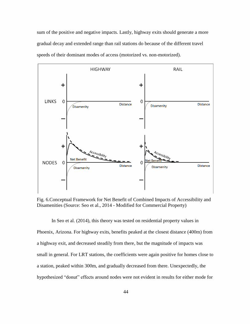
44

sum of the positive and negative impacts. Lastly, highway exits should generate a more

gradual decay and extended range than rail stations do because of the different travel

speeds of their dominant modes of access (motorized vs. non-motorized).

Fig. 6.Conceptual Framework for Net Benefit of Combined Impacts of Accessibility and

Disamenities (Source: Seo et al., 2014 - Modified for Commercial Property)

In Seo et al. (2014), this theory was tested on residential property values in

Phoenix, Arizona. For highway exits, benefits peaked at the closest distance (400m) from

a highway exit, and decreased steadily from there, but the magnitude of impacts was

small in general. For LRT stations, the coefficients were again positive for homes close to

a station, peaked within 300m, and gradually decreased from there. Unexpectedly, the

hypothesized “donut” effects around nodes were not evident in results for either mode for

45

residential property. The proximity to nodes of highways and light rail were highly

significant at the level of 0.001, while the proximity to links of highways and light rail

were not significant even at the level of 0.1. This companion paper tests this model on

commercial property.

Theoretically, we might expect some differences between the effects on

residential and commercial property. First, nuisance effects on commercial property are

hypothesized to be less negative compared with residential property because activities on

commercial property may themselves cause a considerable amount of noise nuisance

(e.g., mechanical noise in industrial property, customer-caused traffic and noise in retail

and service properties) and commercial activities take place in the daytime when

nuisances are more acceptable. In addition, crowds near transportation nodes that may

generate nuisances can be favorable to commercial property but not to residential

property markets. Thus, peaks of the net benefit curves in the Fig. 6 should be skewed

more to the left or there may be no donut effects.

Commercial property can be subdivided into office, industrial, and retail/service

categories, and the impacts of transportation infrastructure are likely to vary by type

(Ryan 1995). According to industrial location theory, transportation cost of inputs and

outputs is one of the most important factors with labor cost and agglomeration economies

(Weber 1929). Thus, for industrial property, it may be more important to locate for

minimizing transportation cost of shipping products and materials rather than to be near

light rail stations3. On the other hand, office property generally does not ship much in the

way of materials and/or products, but employees benefit from light-rail access for daily

3 However, if a freight rail network exists in the study area, industrial property may be found near freight

rail stations to reduce transport cost of inputs and outputs based on the traits of industry.

46

commuting and customers benefit from occasional access as well. Hence, we hypothesize

that office property will put a higher premium on locating near light-rail stations and

highway exits to minimize transportation costs of both customers and employees. Lastly,

retail and service properties need easy access for their employees and customers to

minimize labor cost and maximize profits. Thus, retail and service properties may be

willing to pay more to be located near highway exits and light rail transit stations. In

addition, retail and service properties may prefer to locate in or near a shopping mall for

multi-purpose shopping agglomeration economies.

Methods

This paper extends the methodology developed by Seo et al. (2014) for residential

property to commercial property. This methodology utilizes hedonic regression analysis

to capture the relationships between proximity of transportation infrastructure and

commercial property values while controlling for other determinants of value. To select a

suitable functional form, scatter plots for the variables and log-transformed variables

were analyzed for linearity, and the Akaike Information Criterion (AIC) and Bayesian

Information Criterion (BIC) were examined to compare relative quality of models. To

avoid multicollinearity, the variance inflation factor (VIF) was also examined. For the

goodness of fit, adjusted R² values were compared. Consequently, we selected the

double-log functional form, which has an advantage in estimating price elasticities. It is

expressed as:

(1)

where is the price of commercial property i; is a constant; are structural

characteristics for property i; are neighborhood characteristics for property i; are

47

locational characteristics for property i; and are distance band dummies for property i;

and represent the coefficients of , , , and respectively; and is

random error for property i. The dependent variable is the sale price of commercial

property adjusted by the monthly home price index (HPI; S&P Dow Jones Indices) to

enable use of a multi-year dataset from 2009 to 2014.

Spatial effects were tested with the Lagrange Multiplier (LM) statistic using

spatial weight matrices (Anselin and Rey 2014). To identify and select a suitable spatial

regression model, we tested two different spatial weighting schemes such as contiguity

(i.e., rook and queen contiguity using Thiessen polygons) and distance-based approaches

(i.e., k-nearest neighbor or the Euclidean distance using property points data). These were

compared using pseudo R² and Lagrange Multiplier test results and the model with the

spatial weight matrix using the Euclidean distance approach was selected. The LM error

test value of 15.117 (p = .000) confirmed the presence of spatial dependence in the error

term, while the LM lag test value of 0.328 (p = .57) rejected the presence of spatial

dependence in dependent variable. The Koenker-Bassett test value of 52.815 (p = .000)

confirmed the heteroscedasticity in the dataset. Thus the spatial error model with

heteroscedasticity option was selected for this study. Equation (2) and (3) provide the

general forms of spatial error model:

(2)

(3)

where is a vector of property sales prices; is the constant term; is the n×1 vector of

the coefficients of the explanatory variables; is the n×1 vector of spatially

48

autoregressive errors; is the coefficient on the spatially lagged error; is the spatially

lagged portion of the error; and is an independent but heteroscedastically distributed

error. Regression analyses were carried out separately for commercial property as a

whole, office property, industrial property, and retail and service properties because

impacts of the proximity of highways and LRT may differ by type of commercial market.

Study Area and Data

Study Area

The City of Phoenix, Arizona was selected as the study area because one of the

study purposes is to compare the results for commercial property to Seo et al. (2014)’s

residential property model. The City of Phoenix is the center of commercial property

markets in the Greater Phoenix Area, where most of the high-rise office buildings are

located (Fig. 7). Phoenix is also the most active industrial property market in the Greater

Phoenix Area (Colliers International 2015). As of 2014 there were 47,882 commercial

property parcels within the city limits, excluding some properties categorized as

commercial but used for residential purposes (e.g., apartment, condos, and multifamily

homes).

Phoenix is an automobile-centered city that is well connected by highways and

grid-style arterials. Though there are multiple strong commercial centers across the city,

downtown Phoenix is the original core of the city and some cultural, commercial, and

governmental activities are still concentrated there. Light rail transit (LRT) opened in

2008 and runs east and north of the central business district (CBD) through job-rich

corridors. Freeways encircle the CBD and extend east, west, and north from downtown.

Phoenix Sky Harbor Airport is one of the most centrally located major airports in the

49

United States, just a few miles east of the CBD and connected to the light rail by an

elevated, automated rubber-tired people mover. Thus, many commercial properties are

located along these arterials, highways, and LRT networks, but relatively more

commercial properties are located near the CBD and airport. In terms of noise

disamenity, commercial properties along the highways are not protected by sound walls,

while all the residential properties are protected by sound walls or earth berms.

Data

Commercial property sales data were obtained from the Maricopa County

Assessor’s Office for use as the dependent variable for this study. This dataset contains

sale prices and dates for commercial properties that were sold between 2009 and 2014,

and also includes structural characteristics such as parcel size, total interior area, a

number of stories, building condition, and construction year. Initially, 8,159 commercial

properties were extracted from the Assessor’s 2015 data. We first removed from the

dataset 3,280 properties used for residential purposes. We also removed some

commercial properties that sold for less than $50,000, which we considered outliers. We

also removed properties with insufficient information. Lastly, we found many cases of

duplicated prices for groups of neighboring properties were sold as a bundle with a single

combined sale price. Rather than delete them from the study, we assigned a proportional

sale price to each parcel prorated by limited property value (LPV) for each member

parcel provided by Assessor's office.

The remaining 3,642 observations were further divided into 1,214 office

properties, 360 industrial properties, and 2,068 retail and service properties. For the

dependent variable, inflation-adjusted sale prices were calculated by using the home price

50

index (HPI) for the city of Phoenix (S&P Dow Jones Indices). The 2010 tract-level

median household income and population density were obtained from the U.S. Census

Bureau to represent neighborhood characteristics. Locational characteristics such as

Euclidean distance to downtown Phoenix, Sky Harbor Airport, shopping malls, and major

arterials were measured using ArcGIS 10.2.2 software and readily available GIS datasets

(see Table 3 for summary of variables).

To develop the best model for testing the transportation amenity/disamenity

hypotheses, many different distance measurements in terms of distance bands and

distance extended ranges were tested (Table 4 and Fig.8 for multiple distance band

approach). Euclidean rings were used to measure all distances. Distances from highway

links were measured in three bands, out to 350m as the noise disamenity zone (Nelson

1982).4 The distance from a highway exit to each commercial property was measured in

sixteen 300m bands, out to 4800m (about 3 miles). The distance from LRT stations to

individual commercial properties was measured in five 300m bands, out to 1500m (about

0.94 miles), and distances from the LRT track were measured in 100m bands, out to

300m (0.18 miles).

4 In Nelson (1982)’s review paper, 300m or 1000feet is considered as a noise zone. However, we used

350m as the impact zone because highway centerline was used to measure distance. Thus three multiple

bands are 0-150m, 150-250m, and 250-350m.

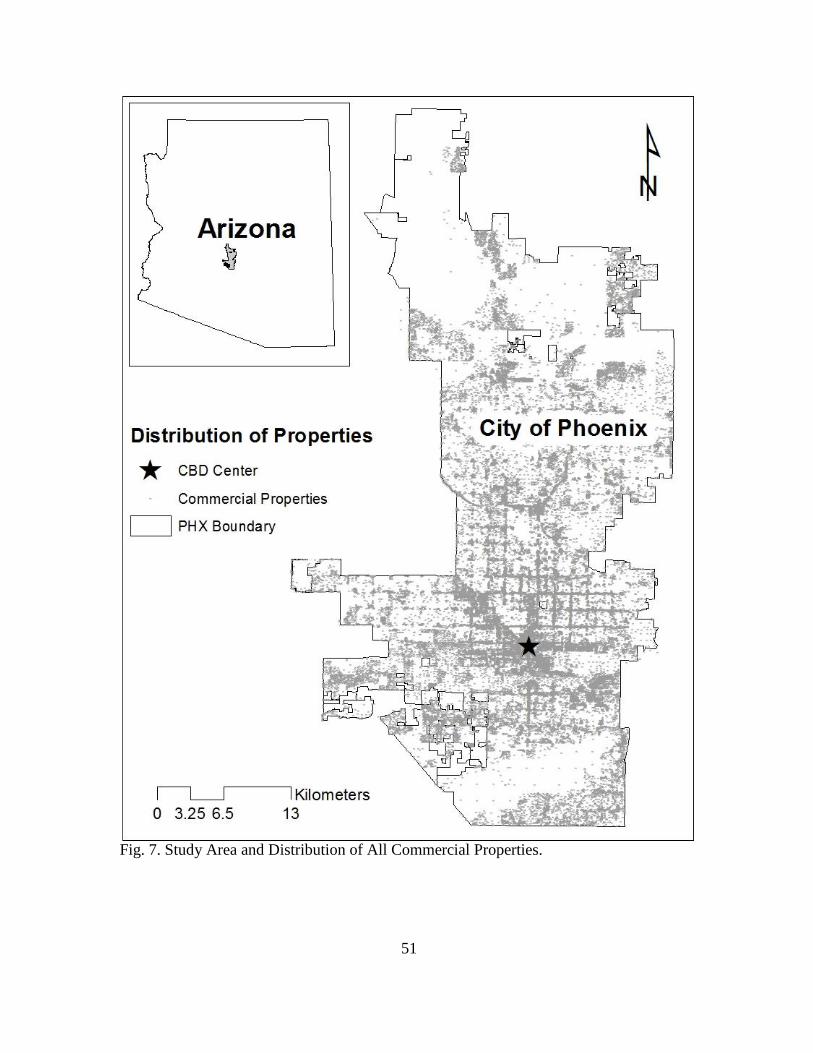
51

Fig. 7. Study Area and Distribution of All Commercial Properties.

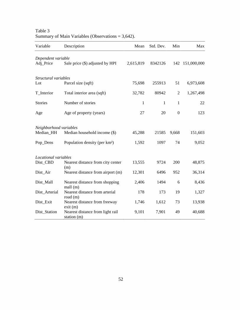
52

Table 3

Summary of Main Variables (Observations = 3,642).

Variable Description Mean Std. Dev. Min Max

Dependent variable

Adj_Price Sale price ($) adjusted by HPI 2,615,819 8342126 142 151,000,000

Structural variables

Lot Parcel size (sqft) 75,698 255913 51 6,973,608

T_Interior Total interior area (sqft) 32,782 80942 2 1,267,498

Stories Number of stories 1 1 1 22

Age Age of property (years) 27 20 0 123

Neighborhood variables

Median_HH Median household income ($) 45,288 21585 9,668 151,603

Pop_Dens Population density (per km²) 1,592 1097 74 9,052

Locational variables

Dist_CBD Nearest distance from city center

(m)

13,555 9724 200 48,875

Dist_Air Nearest distance from airport (m) 12,301 6496 952 36,314

Dist_Mall Nearest distance from shopping

mall (m)

2,406 1494 6 8,436

Dist_Arterial Nearest distance from arterial

road (m)

178 173 19 1,327

Dist_Exit Nearest distance from freeway

exit (m)

1,746 1,612 73 13,938

Dist_Station Nearest distance from light rail

station (m)

9,101 7,901 49 40,688

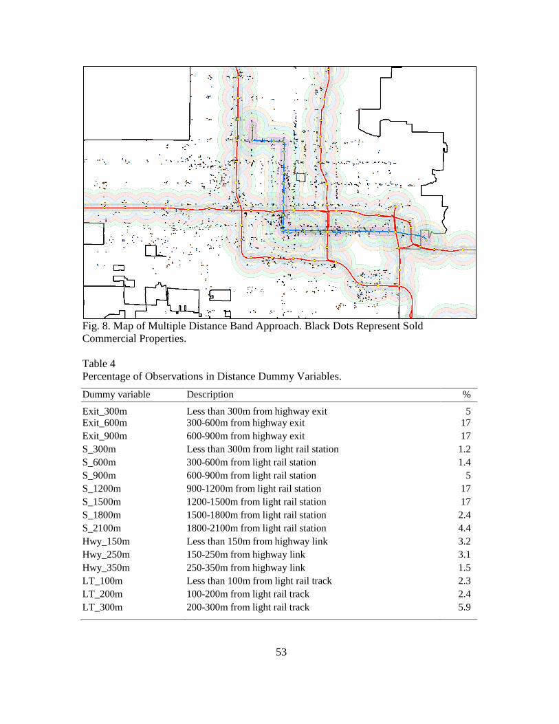
53

Fig. 8. Map of Multiple Distance Band Approach. Black Dots Represent Sold

Commercial Properties.

Table 4

Percentage of Observations in Distance Dummy Variables.

Dummy variable Description %

Exit_300m Less than 300m from highway exit 5

Exit_600m 300-600m from highway exit 17

Exit_900m 600-900m from highway exit 17

S_300m Less than 300m from light rail station 1.2

S_600m 300-600m from light rail station 1.4

S_900m 600-900m from light rail station 5

S_1200m 900-1200m from light rail station 17

S_1500m 1200-1500m from light rail station 17

S_1800m 1500-1800m from light rail station 2.4

S_2100m 1800-2100m from light rail station 4.4

Hwy_150m Less than 150m from highway link 3.2

Hwy_250m 150-250m from highway link 3.1

Hwy_350m 250-350m from highway link 1.5

LT_100m Less than 100m from light rail track 2.3

LT_200m 100-200m from light rail track 2.4

LT_300m 200-300m from light rail track 5.9

54

Results

All Commercial Property

Table 5 shows the coefficients, significance levels, Pseudo R², and Lambda (

for the spatial error models for all commercial properties and for three commercial

property submarkets (see APPENDIX C to F for details) 5

. The Pseudo R² (.792) of

spatial error model and the R² (.791) of standard OLS model are similar and exceed the

range of published results (i.e., R² of 0.33 – 0.73) of other hedonic studies of commercial

property (Clapp 1980; Ryan 1995; Dunse and Jones 1998; Golub et al., 2012). Overall,

most of the control variables are highly significant at the 0.001 level and the signs are as

expected except for population density.

5 Hedonic models were estimated with and without the 2009 data because of the sharp fluctuations of the

real estate market caused by financial crisis. Results, however, did not differ substantially, and therefore the

final results included all years of data.

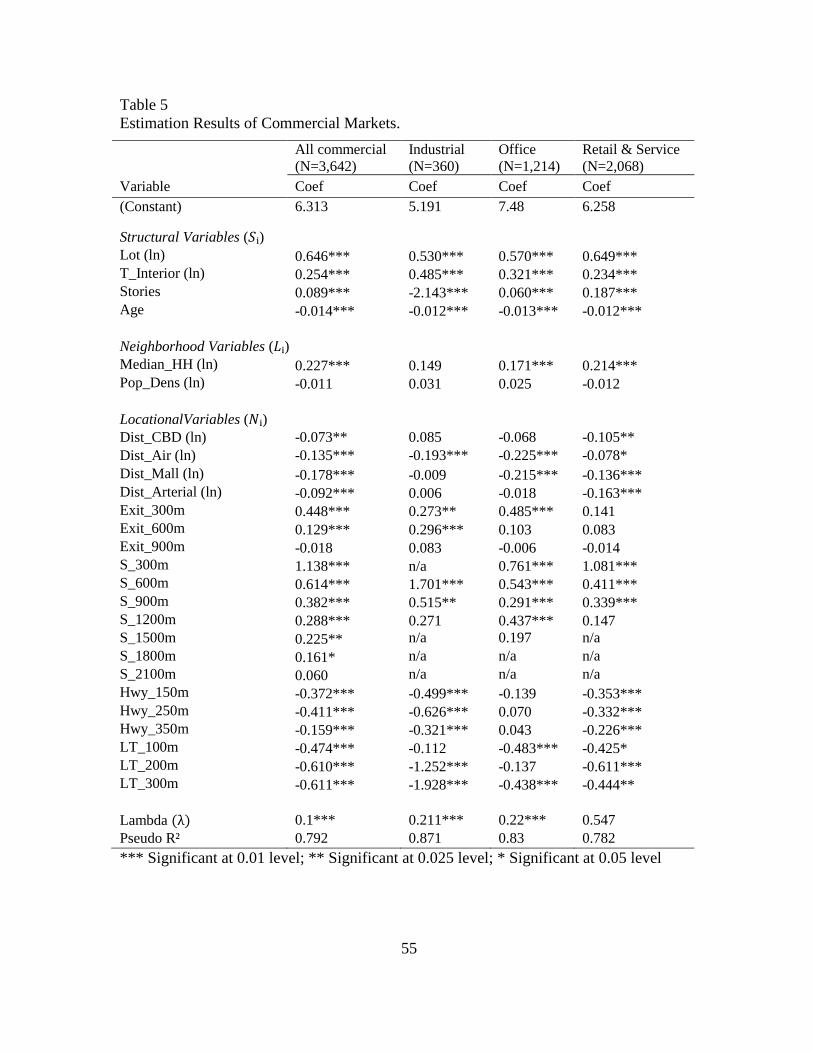
55

Table 5

Estimation Results of Commercial Markets.

All commercial

(N=3,642)

Industrial

(N=360)

Office

(N=1,214)

Retail & Service

(N=2,068)

Variable Coef Coef Coef Coef

(Constant) 6.313 5.191 7.48 6.258

Structural Variables ( )

Lot (ln) 0.646*** 0.530*** 0.570*** 0.649***

T_Interior (ln) 0.254*** 0.485*** 0.321*** 0.234***

Stories 0.089*** -2.143*** 0.060*** 0.187***

Age -0.014*** -0.012*** -0.013*** -0.012***

Neighborhood Variables ( )

Median_HH (ln) 0.227*** 0.149 0.171*** 0.214***

Pop_Dens (ln) -0.011 0.031 0.025 -0.012

LocationalVariables ( )

Dist_CBD (ln) -0.073** 0.085 -0.068 -0.105**

Dist_Air (ln) -0.135*** -0.193*** -0.225*** -0.078*

Dist_Mall (ln) -0.178*** -0.009 -0.215*** -0.136***

Dist_Arterial (ln) -0.092*** 0.006 -0.018 -0.163***

Exit_300m 0.448*** 0.273** 0.485*** 0.141

Exit_600m 0.129*** 0.296*** 0.103 0.083

Exit_900m -0.018 0.083 -0.006 -0.014

S_300m 1.138*** n/a 0.761*** 1.081***

S_600m 0.614*** 1.701*** 0.543*** 0.411***

S_900m 0.382*** 0.515** 0.291*** 0.339***

S_1200m 0.288*** 0.271 0.437*** 0.147

S_1500m 0.225** n/a 0.197 n/a

S_1800m 0.161* n/a n/a n/a

S_2100m 0.060 n/a n/a n/a

Hwy_150m -0.372*** -0.499*** -0.139 -0.353***

Hwy_250m -0.411*** -0.626*** 0.070 -0.332***

Hwy_350m -0.159*** -0.321*** 0.043 -0.226***

LT_100m -0.474*** -0.112 -0.483*** -0.425*

LT_200m -0.610*** -1.252*** -0.137 -0.611***

LT_300m -0.611*** -1.928*** -0.438*** -0.444**

Lambda 0.1*** 0.211*** 0.22*** 0.547

Pseudo R² 0.792 0.871 0.83 0.782

*** Significant at 0.01 level; ** Significant at 0.025 level; * Significant at 0.05 level

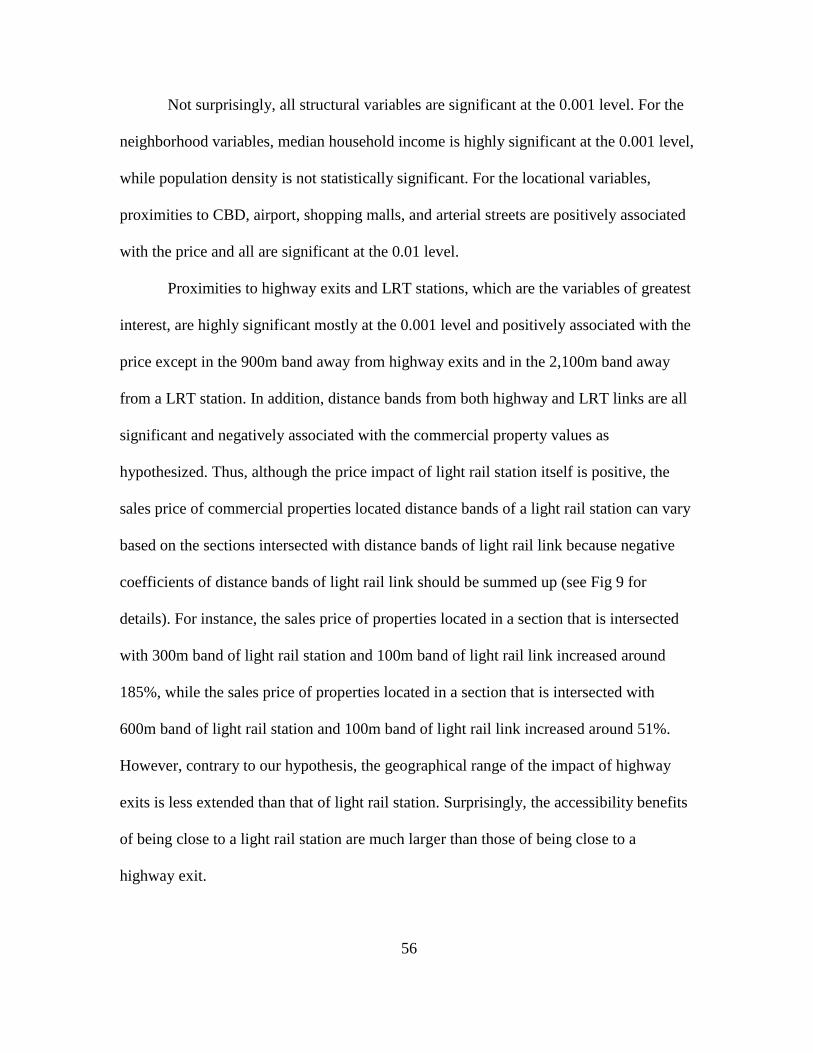
56

Not surprisingly, all structural variables are significant at the 0.001 level. For the

neighborhood variables, median household income is highly significant at the 0.001 level,

while population density is not statistically significant. For the locational variables,

proximities to CBD, airport, shopping malls, and arterial streets are positively associated

with the price and all are significant at the 0.01 level.

Proximities to highway exits and LRT stations, which are the variables of greatest

interest, are highly significant mostly at the 0.001 level and positively associated with the

price except in the 900m band away from highway exits and in the 2,100m band away

from a LRT station. In addition, distance bands from both highway and LRT links are all

significant and negatively associated with the commercial property values as

hypothesized. Thus, although the price impact of light rail station itself is positive, the

sales price of commercial properties located distance bands of a light rail station can vary

based on the sections intersected with distance bands of light rail link because negative

coefficients of distance bands of light rail link should be summed up (see Fig 9 for

details). For instance, the sales price of properties located in a section that is intersected

with 300m band of light rail station and 100m band of light rail link increased around

185%, while the sales price of properties located in a section that is intersected with

600m band of light rail station and 100m band of light rail link increased around 51%.

However, contrary to our hypothesis, the geographical range of the impact of highway

exits is less extended than that of light rail station. Surprisingly, the accessibility benefits

of being close to a light rail station are much larger than those of being close to a

highway exit.

57

Fig. 9. Summed Up Price Impacts Near Light Rail Station Area. Black Dots Represent

Sold Properties.

One possible explanation for this could be that high speed of motorized vehicles

used for highway access overcomes the physical distance barrier over quite a long range

(e.g., 2-3miles and this covers 88-96% of observations) and this makes accessibility

benefit of most area fairly similar, which in turn lessens the impact except for areas very

close to highway exit (i.e., within 600m). In contrast, access to light rail station is mostly

58

made by non-motorized modes (walk and bike), meaning that distance really matters for

those who live near light rail station for commuting, shopping, and other activities. Thus

the price premium of being close to light rail station accrues right at the station and

declines steeply from there. Surprisingly, the geographical extent of the effect of LRT

stations reaches much farther (i.e., 1800m or 1.12mile) and the magnitude of impacts are

much larger than we expected.

Compared with the results of Seo et al.’s (2014) residential model, the coefficients

of accessibility of commercial property to highway exits are much less extended

geographically and there is no "donut" effect for both results. Impacts of accessibility to

LRT stations are also less extended for commercial than for residential property (see Fig.

10 and Fig. 11).

Fig. 10. Coefficients of Distance to Highway Exits.

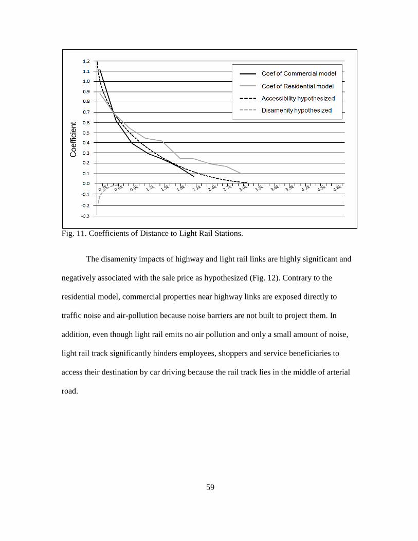
59

Fig. 11. Coefficients of Distance to Light Rail Stations.

The disamenity impacts of highway and light rail links are highly significant and

negatively associated with the sale price as hypothesized (Fig. 12). Contrary to the

residential model, commercial properties near highway links are exposed directly to

traffic noise and air-pollution because noise barriers are not built to project them. In

addition, even though light rail emits no air pollution and only a small amount of noise,

light rail track significantly hinders employees, shoppers and service beneficiaries to

access their destination by car driving because the rail track lies in the middle of arterial

road.

60

Fig. 12. Coefficients of Distance to Highway and Light Rail Links (Residential Results

are not Shown because Coefficients were not Significantly Different from Zero).

Industrial Property

For industrial property, the resulting model fit is quite strong with the adjusted R

of 0.86 for standard OLS and pseudo R of 0.87 for spatial error models. As with the

model for all commercial property, structural variables such as lot square footage, interior

square footage, number of stories, and age of property are all significant at the 0.001 level

and unexpectedly the number of stories is negatively associated with the price (see Table

5). All neighborhood variables factored insignificantly in the price. For the locational

variables, only some distance bands are statistically significant. For instance, 300m –

600m distance bands from highway exits and 600m – 900m distance bands from light rail

stations are significant and positively associated with the price, though size of impact of

light rail stations are larger than that of highway exits, partially validating our hypothesis.

61

Disamenity impacts of highways and light rail links are negative and statistically

significant except for the rail_100 dummy variable. In terms of dollar value change,

industrial properties, for instance, located between 300m and 600m from highway exit

that is not intersected with distance bands of highway link increased 34% in property

value, which is equivalent to a $203,295, increase for a property with the median value of

$590,807. Impact ranges of highway exits are similar with other commercial submarkets,

while light rail stations are relatively shorter in extent than other commercial submarkets.

Office Property

The resulting model fit for office property is quite strong with the adjusted R and

pseudo R of 0.83 for both standard OLS and spatial error models. Coefficients of all

structural variables such as lot square footage, interior square footage, number of stories,

and age of property are all highly significant at 0.001 level and the signs are as expected.

For the neighborhood variables, median income is positive and statistically significant at

0.001 level as expected but population density is statistically insignificant. For the

locational variables, proximity to both the airport and to shopping malls are highly

significant and positive in determining price, while proximity to the CBD and arterial

roads are not significant. For the transportation variables, proximity to highway exit is

positive and significant only at the 300m band but being closer to light rail stations is

positively associated with the price up to 1200m. Proximity to light rail links is negative

and significant at 100m and 300m bands, while proximity to highway links is

insignificant, partially validating our hypothesis. In this model, office properties located

within 300m from a highway exit, where the most benefits are accrued, increased 62% in

sale price, all else being equal.

62

Retail and Service Properties

The resulting model fit for retail and service properties is also quite a strong with

an adjusted R of 0.78 for both standard OLS and spatial error models. Structural

variables such as lot square footage, interior square footage, and age of property are again

significant at 0.001 level and signs are as expected. Median household income is

significant and positively associated with the price but population density is not

significant as neighborhood characteristics.

For the locational variables, proximity to the CBD, airport, shopping malls, and

arterial roads are all significant and positive in determining price. Surprisingly, however,

proximity to highway exits is not significant for any distance band, invalidating our

hypothesis. One possible explanation for this may be that the primary travelers are

different from other commercial submarkets. For instance, the main travelers for

industrial and office properties are likely the employees, while for many retail and service

properties the customers may outnumber the employees. Thus, accessibility benefits for

commuting may be an important factor for employees as well as employers to reduce

transportation costs. On the other hand, in an automobile-centered city like Phoenix,

shoppers and service beneficiaries may care less whether the destination property is

located near a highway exit, because high speed of car driving and grid-like arterial

networks overcome physical distance of 1 or 2miles quite easily, though accessibility is

still important to all travelers. Contrary to highway exits, proximity to light rail stations

are positive and highly significant at distance bands up to 900m, validating our

hypothesis.

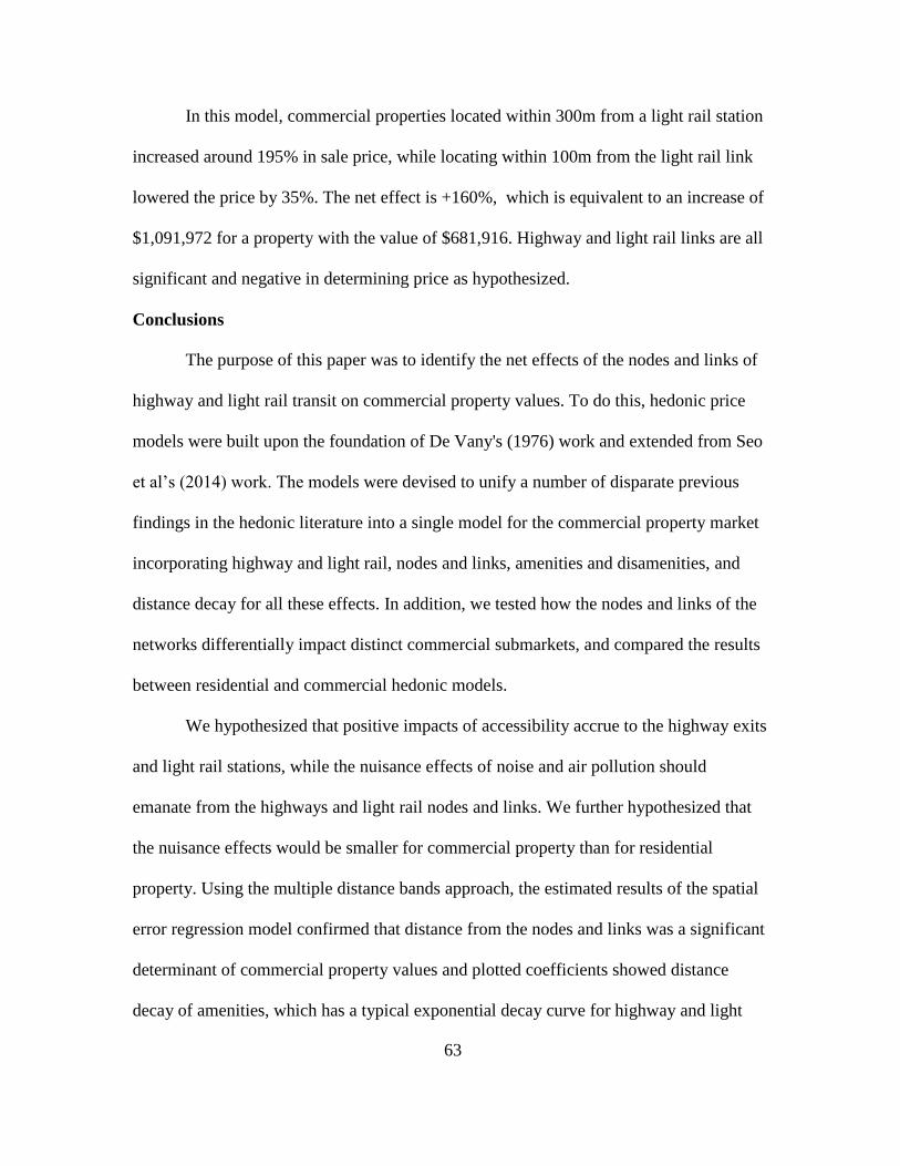
63

In this model, commercial properties located within 300m from a light rail station

increased around 195% in sale price, while locating within 100m from the light rail link

lowered the price by 35%. The net effect is +160%, which is equivalent to an increase of

$1,091,972 for a property with the value of $681,916. Highway and light rail links are all

significant and negative in determining price as hypothesized.

Conclusions

The purpose of this paper was to identify the net effects of the nodes and links of

highway and light rail transit on commercial property values. To do this, hedonic price

models were built upon the foundation of De Vany's (1976) work and extended from Seo

et al’s (2014) work. The models were devised to unify a number of disparate previous

findings in the hedonic literature into a single model for the commercial property market

incorporating highway and light rail, nodes and links, amenities and disamenities, and

distance decay for all these effects. In addition, we tested how the nodes and links of the

networks differentially impact distinct commercial submarkets, and compared the results

between residential and commercial hedonic models.

We hypothesized that positive impacts of accessibility accrue to the highway exits

and light rail stations, while the nuisance effects of noise and air pollution should

emanate from the highways and light rail nodes and links. We further hypothesized that

the nuisance effects would be smaller for commercial property than for residential

property. Using the multiple distance bands approach, the estimated results of the spatial

error regression model confirmed that distance from the nodes and links was a significant

determinant of commercial property values and plotted coefficients showed distance

decay of amenities, which has a typical exponential decay curve for highway and light

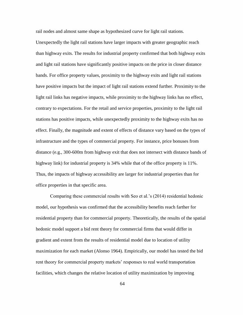
64

rail nodes and almost same shape as hypothesized curve for light rail stations.

Unexpectedly the light rail stations have larger impacts with greater geographic reach

than highway exits. The results for industrial property confirmed that both highway exits

and light rail stations have significantly positive impacts on the price in closer distance

bands. For office property values, proximity to the highway exits and light rail stations

have positive impacts but the impact of light rail stations extend further. Proximity to the

light rail links has negative impacts, while proximity to the highway links has no effect,

contrary to expectations. For the retail and service properties, proximity to the light rail

stations has positive impacts, while unexpectedly proximity to the highway exits has no

effect. Finally, the magnitude and extent of effects of distance vary based on the types of

infrastructure and the types of commercial property. For instance, price bonuses from

distance (e.g., 300-600m from highway exit that does not intersect with distance bands of

highway link) for industrial property is 34% while that of the office property is 11%.

Thus, the impacts of highway accessibility are larger for industrial properties than for

office properties in that specific area.

Comparing these commercial results with Seo et al.’s (2014) residential hedonic

model, our hypothesis was confirmed that the accessibility benefits reach farther for

residential property than for commercial property. Theoretically, the results of the spatial

hedonic model support a bid rent theory for commercial firms that would differ in

gradient and extent from the results of residential model due to location of utility

maximization for each market (Alonso 1964). Empirically, our model has tested the bid

rent theory for commercial property markets’ responses to real world transportation

facilities, which changes the relative location of utility maximization by improving

65

accessibility. Together with Seo et al’s (2014) residential model, this study may

contribute to unify a number of disparate previous findings in the hedonic price literature

into a single, general idealized schematic model incorporating road and rail, nodes and

links, amenities and disamenities, and the distance decay functions for all of these effects.

Lastly, the results of this study may be useful to commercial property buyers to

identify the location where net benefit of accessibility is maximized. Commercial

property construction companies may be able to decide where to build developments for

maximizing profit and sales by predicting where markets will reward location the most.

On the other hand, transportation planners may be able to secure and distribute tax

revenue based on the positive and negative effects captured by the study. City authorities

may possibly use these results as a basis for value capture and tax increment financing of

transportation projects, which depend on knowing the size and extent of benefits to

nearby property.

66

CHAPTER 4

PAVEMENT CONDITION AND PROPERTY VALUES

Abstract

This paper estimates the relationship between pavement condition and residential

property value in Solano County. We hypothesize that pavement condition impacts

property values: directly as an indicator of neighborhood blight, and indirectly through its

effect on traffic conditions and noise. Both effects are expected to be in the same

direction; as pavement condition declines, property values are expected to decline as

well. Hedonic regression models are used to estimate the contribution of road pavement

condition to home sales value. We developed regression models for the County as a

whole and each city, because Solano County as a whole and each city have different

locational and neighborhood characteristics, which should be addressed for developing

best model specification and figured out whether individual city has a different

relationship between pavement condition and residential home prices. Results for Solano

County models with a full dataset and a surveyed PCI dataset confirm that there is no

significant relationship between pavement condition and residential sales price. However,

separate estimates for the each city are mixed with positive, negative, and zero effects.

Because the contribution of road pavement condition to the value of a home is

inconsistent by models, results cannot be conclusively estimated.

Keywords: PCI, residential home value, hedonic model, pavement condition

67

Introduction

Road pavement condition is directly related to generation of nuisances such as

traffic noise and air pollution, which cause an unpleasant environment and heath issues of

neighborhood adjacent to a road. Pavement management agency spends significant

amount of public expenditure every year to maintain and to reduce the impacts of

nuisances caused by pavement deterioration (Pellecuer et al., 2014). Thus, it may be

worth investigating how pavement condition can influence on the neighborhood welfare

in monetary terms.

Many studies aim to estimate the impacts of environmental or nonmarket goods

on human welfare. A number of economic valuation methods have been developed and

used to estimate these impacts, including contingent valuation models, travel cost models,

and hedonic price models (Champ et al., 2003). In this study, we used the hedonic

approach to estimate the influence of pavement condition on residential property value

using Pavement Condition Index (PCI). PCI represents the structural and material

integrity of a pavement in a numerical value (Gharaibeh et al., 2010). The PCI is

expressed on a scale between 0 and 100, where a value of 100 represents the best possible

condition (Shahin et al., 1978). We develop a hedonic model of property value as a

function of various characteristics of the property, including the PCI on the street. There

are two ways that pavement condition might impact property values: directly as an

indicator of neighborhood blight, and indirectly through its effect on traffic conditions

and noise, which in turn impacts property values. Both effects are expected to be in the

same direction; as pavement condition declines, property values are expected to decline

as well.

68

In the following sections we present the data used and more details about the

model, and its results. First, we reflect on existing work in this area as it informs this

study. Then, after we describe study area, data processing, and examination of PCI data,

we formulate our general regression model and present specific results for the selected

models that can represent relationships between residential property values and PCI. We

finish with a discussion and conclusions.

Literature Review

In this section, we first review the hedonic price model and then review on

existing work in relation to this study. Although we reviewed a research report that is

directly related to this study, we mostly reflected on works that are closely related to this

area such as relationship between pavement condition and traffic noise, impacts of traffic

noise on residential property values, and impacts of traffic speed and noise on health

because there is no peer-reviewed paper in literature.

Hedonic Price Model

The hedonic price model is the most widely used approach. These models

estimate the economic value of nonmarket goods by separating the total value of the good

(for example, real estate) – for which a market price is known – into the value of each of

its characteristics, including “nonmarket” characteristics. Real estate has both

differentiated characteristics (e.g., lot size, living area, number of stories, and number of

rooms) and a location. Variation in the location of real property relative to environmental

amenities (“benefits” i.e. local parks, schools, or transportation accessibility) or

disamenities (“negative impacts” i.e. noise, crime, pollution, or neighborhood blight)

provides the information needed to estimate the impact of those amenities and

69

disamenities on the property’s value. The existing literature generally supports the

hypothesis that neighborhood amenities – including high quality transportation

infrastructure – have a positive influence on property values (e.g., Shultz and King, 2001;

Boyle and Kiel, 2001; Bateman et al., 2001; Salon et al., 2014; Seo et al., 2014), and that

disamenities have a negative impact (e.g., Hite et al., 2001; Nelson, 1982; Li and

Saphores, 2012).

Relationship between Pavement Condition and Property Value

To the best of our knowledge, there is no peer-reviewed study that has directly

estimated the relationship between pavement condition and property values. In one

unpublished study, Rasmussen and Yang (2012) used a hedonic model with regression

analysis to determine the relationship between pavement condition and residential

property values. They investigated whether 1) street improvements resulted in an increase

in property value and 2) the benefits to homeowners outweighed the cost of

pavement/street improvements.

Initially they found that property values decreased with increasing

street/pavement condition and it was significant at the 0.1 level. Then they created home

price indicator variables (i.e., above and below sample mean: $178,384) and interacted

these indicator variables with Street Condition Index (SCI) variable. This interaction

model resulted that property values increased with increasing street/pavement condition

when the home sale prices are above the sample mean (e.g., 1 point increase in SCI

causes to 0.07% increase in home price). However, using the home price indicator

dummy variables in their hedonic models is not valid. The problem is that this introduces

a dummy variable for being in the top half (or bottom half) of the sample, which of

70

course is positively correlated with higher home values. Thus, interacting with these top

or bottom half dummy variables with SCI naturally produces a positive or negative effect

based on the home price indicator variables. Instead of using home price indicator

dummy variables, they should ran an interaction model with a dependent variable of top

half or bottom half to avoid this issue.

Relationship between Pavement Condition and Traffic Noise

Many studies have investigated the impact of traffic noise on property values

(e.g., Nelson 1978; Nelson 1982; Bateman et al., 2001). Traffic noise is closely related to

the pavement condition because one of the two main components6 of traffic noise is the

friction between vehicle tires and the paved road surface (Mun et al., 2007).

There is substantial evidence that traffic noise increases with declining pavement

condition, which happens as pavements age (Bendtsen et al., 2010a; ADOT, 2012; TRB,

2013). The PCI provides information about pavement aging by including measures of

distress, levels of severity, and distress density. That said, it is important to note that

pavement-related traffic noise is also influenced by factors such as pavement materials

(e.g., asphalt concrete, Portland cement concrete or rubberized asphalt concrete),

pavement texture types (e.g., longitudinal or transverse tine), traffic volume, vehicle

types (e.g., truck or passenger car), and vehicle speed (Mun et al., 2007). In areas where

these additional factors do not vary substantially but pavement quality does, the PCI may

be a good proxy for measures of traffic noise.

6The other component is the vehicle power-train operation. In recent years, power-train noise has been

substantially reduced due to consumer demand for quieter vehicles (Sandberg 2001).

71

Impact of Road Noise on Residential Property Value

The hedonic modeling literature includes many studies of the traffic noise impacts

on property values (e.g., Vessali 1996; Bateman et al., 2001). In fact, traffic noise near

the highway network was the main focus of many of the first transportation related

hedonic studies. Nelson (1982) reviewed and summarized nine empirical hedonic studies

focusing on the nuisance of traffic noise, with the result that highway traffic noise is

estimated to have a negative impact on residential property values. Studies that included

the traffic noise from arterial roads came to the same conclusion (Kawamura and

Mahajan 2005; Sebastian and Wolfgang 2011).

Hedonic studies typically use property sales prices as the dependent variable as

well as explanatory variables representing characteristics of the properties (e.g., lot size,

living area size, number of rooms, number of stories, age of building), the neighborhoods

where they are located (e.g., median household income, population density, proximity of

neighborhood park or open space), and the location of that neighborhood within a larger

region (e.g., school district, distance to the central business district, proximity of

transportation infrastructure) (Bateman et al., 2001). However, since there are no

predetermined characteristics that are suitable for all hedonic models, knowledge of the

local property markets and prior empirical studies are essential to define potentially

important factors (Champ et al., 2003). Especially important factor is how variables of

interest (i.e., pavement condition index in this study) are measured and how that may

affect models using those data.

To measure traffic noise, some researchers used field measurement data in

decibels (dB) or traffic volumes (Gamble, 1974; Sebastian and Wolfgang 2011; Li and

72

Saphores, 2012), while others used a certain distance from the roads (i.e., 1000ft or

300m) as a noise impact zone (Langley 1976; Kim et al., 2007; Seo et al., 2014). Noise

levels measured in decibels are clearly more accurate than other approaches such as

traffic counts or impact zones. However, measuring actual decibels of noise at the parcel

level is expensive. This issue led to the use of alternative approaches such as distance

measures as a proxy for field measurement of the noise nuisance (Bailey, 1977); the

traffic noise effect decays with distance according to a logarithmic scale and fades away

within 1000ft of the noise source (Nelson, 1982). Traffic noise emanates not only from

link of network but node (e.g., highway exits and rail stations) as well, though negative

noise effects of node are usually offset by benefit of accessibility (Seo et al 2014). These

two sources of noise nuisance should be considered simultaneously when impacts

analyses including these factors are done.

Although previous studies revealed 1000ft or 300m as an impact zone along road

links, the actual extent of the impact zone depends on the road configuration (i.e.,

overpass or underpass), the presence of a sound wall or earth berm, the traffic volume,

the types of vehicles passing by, and the pavement condition. Seo et al. (2014) included

both the highway configuration and the distance from the road in their hedonic model to

determine whether residential property values respond differently to elevated, below-

grade, or at-grade highways. Their results showed that below-grade highways have less

impact than at-grade highways, though the impact from elevated highways was not

statistically significant (Seo et al., 2014). Li and Saphores (2012) examined impacts of

truck traffic along highway links in Los Angeles, CA using a multiple distance band

approach (i.e. within100m, 100-200m, and 200-400m) to identify impact zones. Their

73

results show that the residential properties located within the 100-200m band experience

more negative impact than those located within the 200-400m band, though the effect on

properties closest to the highway (within 100m) was not statistically significant (Li and

Saphores, 2012).

Impact of Traffic Speed and Traffic Noise on Health

One mechanism for connecting pavement condition to community impacts and

conditions is through health impacts. Degraded pavement condition may lead to reduced

speeds, and/or increased incidence of deceleration and acceleration. Either of these

occurrences could lead to increased vehicle emissions (Zhang et al., 2011). Vehicle

emissions are a primary source of air pollutants in urban and suburban areas (TRB, 2002)

and these emissions can contribute to a wide range of health impacts, from cardiovascular

problems to adverse birth outcomes and diminished male fertility (WHO, 2005). Indoor,

residential air quality is related to distance from roads (Lawson et al., 2011), which

means that health impacts from degraded air quality will be greatest near roads with

heavy or congested traffic. It is likely that improved pavement condition and other factors

affecting free circulation of traffic could reduce these emissions and incidence of related

health impacts.

Based on the literature review, we found that there is no peer-reviewed study on

relationship between pavement condition and home sales price. Pavement condition,

however, is related to other factors such as noise nuisance that has been studied. In

addition, PCI differs from most transportation infrastructure that has been studied in

hedonic literature, such as rail or highway, because PCI is estimated on every street.

74

Thus, it is not a question of how far away is the transport network, but what is its

condition.

Study Area and Data

Study Area

Solano County, CA is located in the northeastern part of San Francisco Bay Area

and contains 7 incorporated cities: Vallejo, Vacaville, Fairfield, Suisun City, Benicia,

Dixon, and Rio Vista (see Fig. 13). Solano County had a population of 413,344 according

to the 2010 U.S. Census Bureau and has 105,249 single family residential parcels in 2015

based on the County Assessor's data. Interstate highway 80 and an Amtrak rail line cut

through the County. The pavement condition of road segments is surveyed at regular

intervals. Estimated values are also available for the months between surveys, and are

based on a pavement deterioration model.

Data Processing

Data come from multiple sources including Solano County assessor's office,

Solano Transportation Authority (STA), and ESRI web maps. Full details provided in

Table 6.

To conduct this analysis, it is necessary to obtain sales price, assessor-based

single family parcel and home characteristics, and nearby road PCI for all included

properties. The STA provided GIS data necessary to discover relationships between

single family home sales prices and PCI. With these GIS data sets variables were created

for hedonic regression analysis. Additional data sets were created using satellite imagery

for explanatory variables such as highway exits, central business district (CBD), and

water feature classes.

75

For the dependent variable of home price, we used the property sales records

provided by STA. The original dataset contained 34,000 property sales records that

included addresses, sale prices, and sale dates, but were not connected by parcel number

to the assessor dataset that contains detailed information about each property. Through a

text-based address-matching routine, 31,038 of these records were successfully merged

with the assessor data. Records of non-single family homes were removed.

Table 6

List of Data Provided

Data File type Feature type Core attributes Source

34,000 home sales

price

.shp Point Property address

Sold date

Sold price

STA

Parcel_2015 .shp Polygon APN

X, Y coordinates

Structural characteristics

Property address

Assessor's

Office

Road PCIs .shp Line PCI date

PCI

Estimated PCI (2009-

2015)

STA

County boundary .shp Polygon STA

City boundary .shp Polygon STA

Park .shp Point

/Polygon

STA

TransitHub .shp Point STA

Airports .shp Point STA

Landfills .shp Point STA

School .shp Point STA

Capitol station .shp Point STA

Highway .shp Line STA

Amtrak Corridor .shp Line STA

Express bus route .shp Line STA

Contour .shp Line STA

76

Additional challenges required us to discard approximately one-third of the

remaining sales observations. These included missing structural information about the

property, lack of PCI values for the road segments adjacent to the property, and

properties that were sold multiple times in the study period were removed. The reason

that multiple sales of the same property cannot be used in this analysis is that our work

uses spatial econometrics to control for spatial error dependence. Using these methods,

spatially identical observations would have complicated the analysis. After cleaning,

19,608 observations remained in the data set (see Fig.13 for study area).

Fig. 13. Study Area and Data Used

77

In addition to these characteristics, tract-level population density and median

household income from the U.S. Census Bureau were included as control neighborhood

characteristics in the analysis. For the locational characteristics, the “near” function in

ArcGIS was used to calculate the Euclidean distance between each property and the

closest Central Business District (CBD), highway exit, highway link, rail station, rail

track, airport, water, park, and landfill. PCI, the variable of most interest in this study,

was assigned to adjacent properties by first creating a buffer around each road, and then

performing a spatial join with the property sale point data. Year and city dummy

variables were created using attributes from the property sales data and city boundary

polygon feature class, respectively. It is important to note that the dependent variable was

adjusted by the home price index (HPI) for San Francisco and San Jose area to control for

the volatility of the real estate market from 2009 to 2015. Table 7 provides descriptive

statistics for the main variables used in this analysis and Table 8 provides a percentage of

observations for each city and year.

78

Table 7

Descriptive Statistics of Main Variables (N = 19,608)

Variable Description Mean Std. Dev. Min Max

HPI_adj_Price Dependent variable 338895.74 153793.99 39584.25 1562303.16

Structural Variable

LOT_Sqft Square footage of

parcel

6901.98 3365.71 650 194277

Living_Sqf Square footage of

interior area

1659.43 628.93 424 6051

Age Age of house 34.43 21.52 0 149

FirePlc_du Fire place (dummy) 0.83 0.38 0 1

N_Rooms Number of rooms 5.57 1.29 2 13

N_Story Second story = 1

(dummy)

0.39 0.49 0 1

Pooldum Presence of Pool 0.0679 0.2515 0 1

GARAGE Square footage of

garage

440.53 149.93 0 4320

Neighborhood Variable

M_HH_Income Median household

income

73887.39 23698.85 14965 145625

POP_dens Population

density/sqml

4418.97 2973.97 36.39 12228.51

PCI_Year_Same Estimated PCI

same year home

sold

61.37 27.01 0 98.40

Locational Variable

CBD Distance to nearest

CBD

3894.47 2119.89 92.22 12236.66

Station Distance to Amtrak

Station

10622.20 5366.96 246.62 32344.42

All_Arterial Arterial road

dummy

0.0214 0.145 0 1

Hwy_exit Distance to

highway exit

2356.92 3631.32 89.93 33623.88

Park Distance to

regional park

551.28 534.27 0.06 5340.33

Rail_300 300m within rail

track

0.02 0.14 0 1

Hwy320 320m within

highway center line

0.10 0.30 0 1

79

Table 8

Percent of Observations for Each City and Year

City % of observations Year % of observations

Vacaville 26 2009 11

Rio Vista 1 2010 19

Dixon 1 2011 19

Vallejo 31 2012 19

Suisun City 8 2013 13

Benicia 5 2014 11

Fairfield 25 2015 9

Solano County 1

PCI Examination

Substantial effort was put into thoroughly examining the PCI data to understand

the relationship between PCI and the other variables used in the hedonic models, and to

diagnose inconsistent PCI coefficients (i.e., sign changes in different models) in the

results of the selected regression models. The data included an estimated PCI value for

each road segment for each year from 2009 to 2015. As explained above, these estimates

are based on periodic field surveys of pavement condition. A pavement condition

deterioration model is used to estimate PCI for any years between field surveys. The data

also included the date and surveyed pavement condition value for the most recent PCI

survey. In the remainder of this section, we highlight some data quality issues that we

encountered when using these PCI data.

First, surveyed PCI values may have measurement errors that could affect the

results of hedonic regressions (Champ et al., 2003). An expert in grading the pavement

condition of each road segment provides the PCI values in years when a road condition

survey was done. The problem is that the same expert does not survey all of the roads in

the County, leading to the possibility of inconsistency in surveyed PCI values. There has

80

recently been a training program for pavement condition surveyors that aims to address

this issue. However, the data we are using spans the period both before and after the

training program.

Second, we found large changes in PCI values between estimated values in one

year and surveyed values in the next. In the case of large PCI increases, it would make

sense that road maintenance and/or capital improvement operations substantially

improved the pavement condition, and then a new pavement survey confirmed it (e.g., an

estimated PCI of 37 in 2013 and a surveyed PCI of 100 in 2014). However, changes in

the opposite direction (e.g., an estimated PCI of 65 in 2010 and a surveyed PCI of 27 in

2011) are problematic because there is no reasonable explanation for them, and one or

both of those PCI values are likely to be far from correct. If the estimated PCI is incorrect

in these cases, it casts doubt on all estimated PCI values in the dataset. There are

891cases in our data where PCI values “jump” downward by more than 20 points from

one year to the next, not including those cases where we know that the reason is a new

PCI survey.

Because of these doubtful estimated PCI values, we ran two regression

models―one with the full dataset including estimated PCI (i.e., 19,608 cases) and

another that is restricted in surveyed PCI dataset (i.e., 2,960 cases). We have identified

cases where year-to-year increases occurred, and marked them as likely additional survey

years. We have also marked year-to-year drops of more than 7 PCI points as likely

additional survey years. This increases our sample size of homes sold in years with

surveyed PCI to more than 5000.

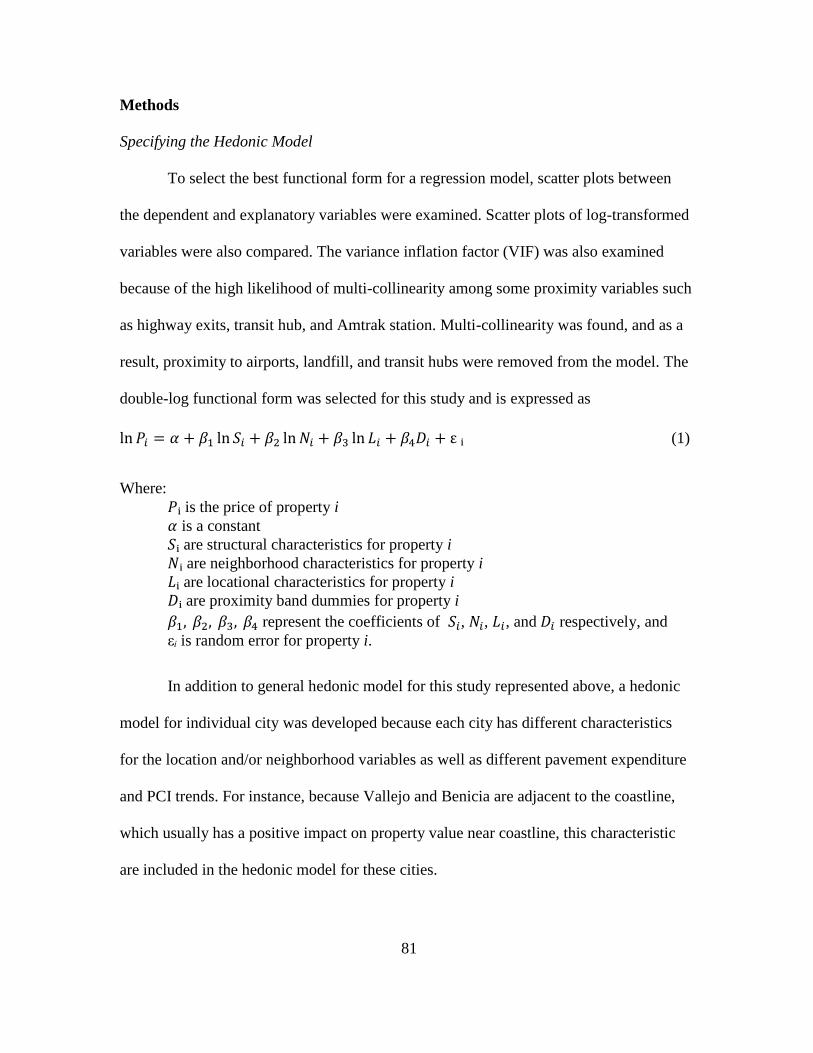
81

Methods

Specifying the Hedonic Model

To select the best functional form for a regression model, scatter plots between

the dependent and explanatory variables were examined. Scatter plots of log-transformed

variables were also compared. The variance inflation factor (VIF) was also examined

because of the high likelihood of multi-collinearity among some proximity variables such

as highway exits, transit hub, and Amtrak station. Multi-collinearity was found, and as a

result, proximity to airports, landfill, and transit hubs were removed from the model. The

double-log functional form was selected for this study and is expressed as

(1)

Where:

is the price of property i

is a constant

are structural characteristics for property i

are neighborhood characteristics for property i

are locational characteristics for property i

are proximity band dummies for property i

represent the coefficients of , , , and respectively, and

is random error for property i.

In addition to general hedonic model for this study represented above, a hedonic

model for individual city was developed because each city has different characteristics

for the location and/or neighborhood variables as well as different pavement expenditure

and PCI trends. For instance, because Vallejo and Benicia are adjacent to the coastline,

which usually has a positive impact on property value near coastline, this characteristic

are included in the hedonic model for these cities.

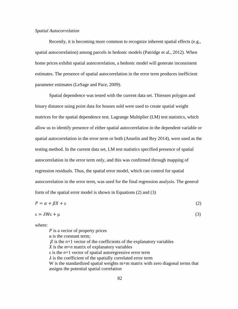
82

Spatial Autocorrelation

Recently, it is becoming more common to recognize inherent spatial effects (e.g.,

spatial autocorrelation) among parcels in hedonic models (Patridge et al., 2012). When

home prices exhibit spatial autocorrelation, a hedonic model will generate inconsistent

estimates. The presence of spatial autocorrelation in the error term produces inefficient

parameter estimates (LeSage and Pace, 2009).

Spatial dependence was tested with the current data set. Thiessen polygon and

binary distance using point data for houses sold were used to create spatial weight

matrices for the spatial dependence test. Lagrange Multiplier (LM) test statistics, which

allow us to identify presence of either spatial autocorrelation in the dependent variable or

spatial autocorrelation in the error term or both (Anselin and Rey 2014), were used as the

testing method. In the current data set, LM test statistics specified presence of spatial

autocorrelation in the error term only, and this was confirmed through mapping of

regression residuals. Thus, the spatial error model, which can control for spatial

autocorrelation in the error term, was used for the final regression analysis. The general

form of the spatial error model is shown in Equations (2) and (3)

(2)

(3)

where:

is a vector of property prices

is the constant term;

is the n×1 vector of the coefficients of the explanatory variables

X is the m×n matrix of explanatory variables

is the n×1 vector of spatial autoregressive error term

is the coefficient of the spatially correlated error term

W is the standardized spatial weights m×m matrix with zero diagonal terms that

assigns the potential spatial correlation

83

is the spatially lagged error terms, and

is independent but heteroskedastically distributed error

Results

All Properties

Initial regression analysis was performed using StataSE 12 for Windows to

determine the best model. The Lagrange Multiplier (LM) test value of 0.056 (p = 0.81)

for lag and 56.21 (p = 0.000) for error confirmed spatial dependence in error term. A

Koenker-Bassett test value of 2203.51 (p = 0.000) confirmed spatial heterogeneity in the

data. Thus, we applied a spatial error model with heterogeneity option using GeoDaSpace

to estimate the coefficients of the independent variables. Table 9 shows the coefficients,

standard error, z-Stat, and significance for the spatial error model. The resulting model fit

is fairly strong with a Pseudo R² of 0.797 and an OLS adjusted R² of 0.79.

Structural variables are all statistically significant at the 0.001 level and all signs

of coefficients are as expected. For instance, number of stories and age of house are

negative and significant, while other structural variables such as home square footage, lot

size, number of rooms, number of fireplaces, presence of pool, and square footage of

garage are all positive and significant as expected.

For neighborhood variables, median household income is positively associated

with property value and highly significant at the 0.001 level, while population density is

negatively associated with property value and highly significant at the 0.001 level. Signs

of the coefficients are as expected.

7 Pseudo R² cannot be interpreted as one would interpret an OLS R², however, a higher Pseudo R²

still can be interpreted as better model fit than a lower one (Anselin 1988).

84

Overall, most of the locational variables are highly significant at the 0.001 level

except distance from highway exit and some of the city dummy variables. For instance,

proximity to the central business district (CBD) and arterial roads, which represent the

accessibility of jobs and transportation, are positively associated with the property values.

Finally, the coefficient of PCI, the variable of the greatest interest, is not

statistically significant. This means that with our data, we cannot detect a relationship

between residential property values and pavement condition adjacent to the home. As

noted earlier, however, the PCI data may contain errors. We also analyze subsamples of

the data set.

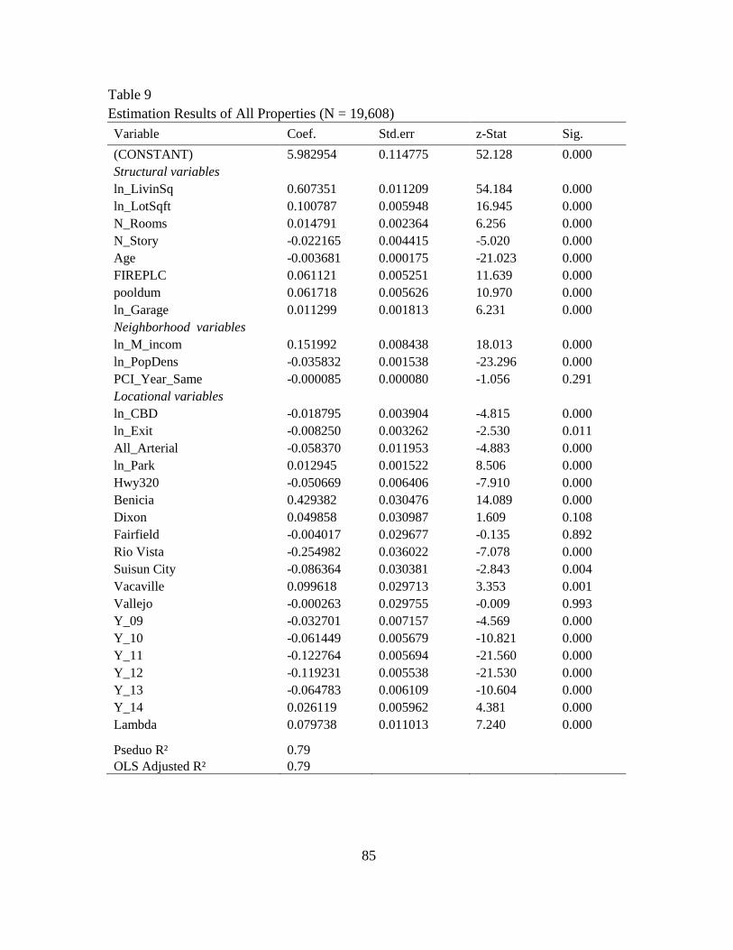
85

Table 9

Estimation Results of All Properties (N = 19,608)

Variable Coef. Std.err z-Stat Sig.

(CONSTANT) 5.982954 0.114775 52.128 0.000

Structural variables

ln_LivinSq 0.607351 0.011209 54.184 0.000

ln_LotSqft 0.100787 0.005948 16.945 0.000

N_Rooms 0.014791 0.002364 6.256 0.000

N_Story -0.022165 0.004415 -5.020 0.000

Age -0.003681 0.000175 -21.023 0.000

FIREPLC 0.061121 0.005251 11.639 0.000

pooldum 0.061718 0.005626 10.970 0.000

ln_Garage 0.011299 0.001813 6.231 0.000

Neighborhood variables

ln_M_incom 0.151992 0.008438 18.013 0.000

ln_PopDens -0.035832 0.001538 -23.296 0.000

PCI_Year_Same -0.000085 0.000080 -1.056 0.291

Locational variables

ln_CBD -0.018795 0.003904 -4.815 0.000

ln_Exit -0.008250 0.003262 -2.530 0.011

All_Arterial -0.058370 0.011953 -4.883 0.000

ln_Park 0.012945 0.001522 8.506 0.000

Hwy320 -0.050669 0.006406 -7.910 0.000

Benicia 0.429382 0.030476 14.089 0.000

Dixon 0.049858 0.030987 1.609 0.108

Fairfield -0.004017 0.029677 -0.135 0.892

Rio Vista -0.254982 0.036022 -7.078 0.000

Suisun City -0.086364 0.030381 -2.843 0.004

Vacaville 0.099618 0.029713 3.353 0.001

Vallejo -0.000263 0.029755 -0.009 0.993

Y_09 -0.032701 0.007157 -4.569 0.000

Y_10 -0.061449 0.005679 -10.821 0.000

Y_11 -0.122764 0.005694 -21.560 0.000

Y_12 -0.119231 0.005538 -21.530 0.000

Y_13 -0.064783 0.006109 -10.604 0.000

Y_14 0.026119 0.005962 4.381 0.000

Lambda 0.079738 0.011013 7.240 0.000

Pseduo R² 0.79

OLS Adjusted R² 0.79

86

Properties with Surveyed PCI

Because the estimated PCI may include errors due to the road deterioration

prediction model over or underestimating the true pavement condition, we estimate our

model on the subset of home sales that occurred in a year when PCI was surveyed. This

subsample includes both home sales that occurred in the year when the PCI was most

recently surveyed – as listed in the dataset – as well as home sales that occurred in a year

for which we presume that the PCI must have been surveyed – based on the year-to-year

patterns of estimated PCI values. Like the full sample, spatial autocorrelation for the error

term was detected in this subsample, confirmed by the LM test value of 0.639 (p = 0.4)

for lag and 80.5 (p = 0.000) for error. A Koenker-Bassett test value of 671.99 (p = 0.000)

also confirmed the presence of heterogeneity in the subsample. Thus, we again applied a

spatial error model with heterogeneity option using GeoDaSpace. Table 10 shows the

results of analysis. The resulting model fit is fairly strong with a Pseudo R² of 0.8 and an

OLS adjusted R² of 0.8.

Overall, the results are not different from the All Property model. For instance,

structural variables are all statistically significant at the 0.01 level except N_Story which

is still statistically significant at the 0.05 level and all coefficients signs are as expected.

For the neighborhood variables, median household income is positively associated with

property value and highly significant at the 0.001 level, while population density is

negatively associated with property value and highly significant at the 0.001 level. Signs

of both coefficients are as expected. For the locational variables, however, some variables

are less significant than the same variables are in the All property model. For instance,

distance to Hwy320 dummy variable is significant at the 0.05 level and distance to

87

All_Arterial is not significant even at the 0.05 level. However, all signs are consistent

with the All property model. The coefficient of PCI is not significant even at the 0.1

level, thus there is no detectable relationship between residential property values and

pavement condition.

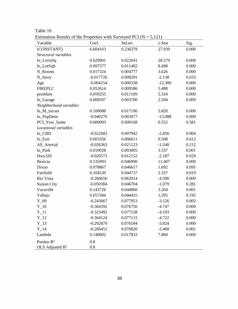
88

Table 10

Estimation Results of the Properties with Surveyed PCI (N = 5,121)

Variable Coef. Std.err z-Stat Sig.

(CONSTANT) 6.604103 0.236379 27.939 0.000

Structural variables

ln_LivinSq 0.629901 0.022041 28.579 0.000

ln_LotSqft 0.097577 0.011482 8.498 0.000

N_Rooms 0.017324 0.004777 3.626 0.000

N_Story -0.017726 0.008291 -2.138 0.033

Age -0.004154 0.000338 -12.306 0.000

FIREPLC 0.052614 0.009586 5.488 0.000

pooldum 0.059255 0.011109 5.334 0.000

ln_Garage 0.009597 0.003700 2.594 0.009

Neighborhood variables

ln_M_incom 0.100088 0.017196 5.820 0.000

ln_PopDens -0.040270 0.003077 -13.088 0.000

PCI_Year_Same 0.000093 0.000168 0.552 0.581

Locational variables

ln_CBD -0.022683 0.007942 -2.856 0.004

ln_Exit 0.003356 0.006611 0.508 0.612

All_Arterial -0.026363 0.021123 -1.248 0.212

ln_Park 0.010028 0.003005 3.337 0.001

Hwy320 -0.026573 0.012152 -2.187 0.029

Benicia 0.535993 0.046990 11.407 0.000

Dixon 0.078867 0.046617 1.692 0.091

Fairfield 0.104530 0.044737 2.337 0.019

Rio Vista -0.284656 0.062014 -4.590 0.000

Suisun City -0.050384 0.046704 -1.079 0.281

Vacaville 0.143726 0.044860 3.204 0.001

Vallejo 0.057584 0.044455 1.295 0.195

Y_09 -0.243667 0.077953 -3.126 0.002

Y_10 -0.364392 0.076756 -4.747 0.000

Y_11 -0.323492 0.077158 -4.193 0.000

Y_12 -0.364124 0.077115 -4.722 0.000

Y_13 -0.292879 0.076594 -3.824 0.000

Y_14 -0.266451 0.076820 -3.468 0.001

Lambda 0.140602 0.017833 7.884 0.000

Pseduo R² 0.8

OLS Adjusted R² 0.8

89

Properties of Each City

As noted previous section, both neighborhood and locational characteristics as

well as pavement related expenditure are different in each city. Thus, some control

variables in specific cities should be removed or added. For example, Rio Vista is a very

small city and around 98% of sold homes are located within 2 miles of one another. This

means that certain neighborhood (e.g., population density) or locational (e.g., distance to

water front) characteristics in Rio Vista are essentially the same for all properties. Thus,

these control variables should be excluded in the regression model.

Table 11 shows a summary of the results for all cities. Some cities such as

Vallejo, Vacaville, Fairfield, Suisun City, and Rio Vista required the spatial error model

with heterogeneity option, while other cities did not. The resulting model fits are

generally strong, with R-squared statistics ranging from 0.64 to 0.86. The relationship

between PCI and property value seemed to differ by city. Like the County-level models

presented earlier, some city models yielded statistically insignificant results such as

Vallejo, Vacaville, and Solano County. PCI results for Dixon and Rio Vista are negative

and significant at the 0.01 and 0.05 level respectively, while Fairfield’s is positive and

highly significant at the 0.001 level. In Suisun City, the relationship between PCI and

home values are positive and somewhat significant at the 0.1 level, while in Benicia the

relationship between PCI and home values are negative and somewhat significant at the

0.1 level (see APPENDIX G to N for full city-specific results tables).

90

Table 11

Estimation Results of Cities

City N =

19608

Model Adj- R²

/Pseudo

R²

PCI

Coef. Std.err z-Stat Sig.

Vallejo 6127 Spatial error/Het 0.70 -0.000199 0.000127 -1.568 0.117

Vacaville 5165 Spatial error/Het 0.77 -0.000135 0.000173 -0.781 0.435

Fairfield 4962 Spatial error/Het 0.86 0.000692 0.000184 3.766 0.000

Suisun

City

1645 Spatial error/Het 0.69 0.000292 0.000159 1.837 0.066

Benicia 971 OLS (no spatial

autocorrelation)

0.75 -0.000409 0.000242 -1.689 0.091

Dixon 279 OLS (no spatial

autocorrelation)

0.81 -0.003663 0.000678 -5.404 0.000

Rio Vista 243 Spatial error/Het 0.64 -0.000931 0.000405 -2.298 0.022

Solano

County

216 OLS (no spatial

autocorrelation)

0.85 0.001273 0.000881 1.444 0.150

Discussion and Conclusions

The purpose of this study was to identify the relationship between residential

property values and pavement condition. We hypothesized that higher PCI is positively

associated with property values. Although there is no peer reviewed literature directly

related to this study, many previous studies have developed hedonic models of

neighborhood blight (Anderson, 1990; Man and Rosentraub, 1998; Dye and Merriman,

2000). We developed hedonic regression models for all properties, properties assigned

surveyed PCI, and for each city. In general, structural, neighborhood, and locational

variables for all models are not significantly different in sign except for in some of the

city-specific models.

However, in terms of PCI, results vary across all models (i.e., positive in 2 cities,

negative in 3 cities, and zeros in 2 cities). We have tried many different combinations

91

such as time periods (2009 - 2011/2012 - 2015), focusing on certain ranges of property

values (high / low), and adding other neighborhood characteristics, but the results

remained basically unchanged. According to this model, pavement condition as

represented by PCI does not appear to have a strong and consistent relationship with

home values in Solano County. Further, the negative signed results are troubling because

there is no reasonable explanation for them – a better road should never diminish the

value of a house. The fact that we obtain these counterintuitive results suggests one or

both of the following: (1) there may be a problem in the data or (2) road pavement

condition is closely related to characteristics of the home or neighborhood that do

diminish the value of a house.

92

CHAPTER 5

CONCLUSIONS

Overview

This dissertation examined the relationship between transportation infrastructure

and property values using spatial hedonic regression models. This dissertation proposed a

generalized and more comprehensive theory of the positive and negative relationships

between transportation infrastructure and real property values, which disentangles

different effects by road and rail, by nodes and links, and by distance from them. A

distance band approach was used to capture effects of non-linear distance function and

distance ranges. None of previous studies have conducted a unified approach as

developed here to differentiate all these effects.

The strongest conclusion drawn from the results of the Chapter 2 and 3 is that

proximity to transport nodes was associated positively with both residential and

commercial property values. As a function of distance from highway exits and LRT

stations, the distance-band coefficients formed a typical positive longer-range distance

decay pattern of accessibility effect but there is no shorter range distance decay of

disamenity effect. As hypothesized, the accessibility effect for highway exits extended

farther than for LRT stations in residential property model, but for commercial property

models the distance range of the two modes was reversed and effect of LRT stations

extended farther than that of highway exits. For both types of property, the magnitude of

accessibility effect for highway exits is smaller than for LRT stations. Unexpectedly, the

hypothesized negative effect on property values immediately surrounding rail stations

and highway exits was not evident for either mode or either property type. As speculated

93

in the relevant chapters, these results may be explained by the inherent characteristics of

property type (tolerance of noise: resident vs. commercial), features not controlled for

(noise barrier), and inaccurately estimated data (point for nodes and centerline for links).

These explanations need to be further investigated.

Coefficients for the distance from highway and LRT links were generally

negative but not significant in the residential model. However, in the all-commercial

model, the coefficients for the distance from highway and LRT links were significant and

negative, as expected. However, coefficients for the distance from highway and LRT

links vary based on the submarket of commercial property. Another results of Chapter 2

for the effect of highway configuration on home values showed that below-grade

highways have relatively positive impacts on nearby houses compared to those at ground

level or above in Phoenix, Arizona. Lastly, the main conclusion that can be drawn from

the results of the analyses presented in Chapter 4 is that pavement condition had no

relationship with the residential property values in Solano County, California.

Implications

This dissertation contributes to the hedonic literature in that Chapter 2 and 3 have

unified a number of disparate previous findings in the hedonic literature into a single

model for residential and commercial property markets (Golub et al, 2012), incorporating

highway and light rail (Bowes and Ihlanfeldt 2001; Ryan 2005; Andersson et al, 2010),

nodes and links (Kilpatrick et al, 2007; Andersson et al, 2010), and distance decay of all

these effects. Theoretically, the results of Chapter 2 and 3 support Alonso's bid rent

theory for residential and commercial property markets, and also support a bid rent theory

for commercial properties that differs somewhat in gradient and extent from the results of

94

residential property model due to location of utility maximization for each market

(Alonso 1964). The results of Chapter 2 and 3 may be useful to property buyers to

identify the location where net benefit of accessibility is maximized. Real-estate

developers may be able to decide where best to build real estate for maximizing benefit

by predicting where markets will reward location the most. Transportation planners, on

the other hand, may be able to secure and distribute tax revenue based on the positive and

negative effects captured by this dissertation. City authorities could use these results as a

basis for value capture and tax increment financing of transportation projects, which

depend on knowing the size and extent of benefits to nearby property.

Chapter 4 contributes to the hedonic literature by analyzing the relationship

between home values and road pavement condition, which has not been published in the

peer-reviewed literature yet. A small but positive effect of pavement condition on home

values was hypothesized. Despite testing several different model formulations, no

significant positive relationship was found. These non-significant results need to be

confirmed by other studies, which would be important for public policy in terms of

whether housing values are a valid justification for street maintenance.

Future Research

The three individual articles presented in this dissertation untangled relationships

between property values and transportation infrastructure that is invested for

accessibility, mobility, and economic development. However, not all results are as

hypothesized and there may be reasons why some results are not correspond with

hypotheses. Specifically, donut effect from highway exits and LRT stations has not been

found in both residential and commercial property models. Besides, negative effect from

95

highways and LRT links was not captured in residential property model, while it was

captured in commercial property model. One possible reason is the data used for highway

links and exits, which have non-negligible width (e.g., width of highway links is about

35-90m and width of some highway interchanges is about 160m), and the traffic noise

effect decays with distance based on a logarithmic scale and fades away within 300m of

the noise source (Nelson, 1982). Using the centerlines of highway and the points of exit

cannot measure the exact distance from the properties to the edge of the highway nodes

and links. Thus, further research may be required to investigate with more accurate data

why proximity to the links—which theoretically should have a primarily negative

disamenity from noise and air pollution and no positive accessibility effect— and

proximity to the exits—which theoretically should have a net effect of accessibility and

disamenity— was not captured for highway and rail in Chapter 2.

Since light rail transit is a new type of transport investment in Phoenix, it may be

interesting to study how this investment influences land use, population, employment,

walkability, and property values in geographical extent. By comparing those factors in

terms of pre-LRT and post-LRT periods, impacts and service area of stations might be

identified and validity of LRT investment might be supported. Furthermore, it may be

valuable to investigate whether sidewalk or bike infrastructure positively impacts on

property markets including single- and multi-family home and commercial property,

because walkability has been proved to increase home values in some cities in the U.S.

and Canada where walkability is increased (Cortright 2009; Chad 2012; Li et al, 2015).

In relation to road pavement, the City of Phoenix has applied new pavement

material (e.g., rubberized asphalt) to roads to reduce traffic noise. This can be an

96

interesting subject of future study. Because quiet pavement can reduce traffic noise about

5.1 dB, reduction of noise level may positively affect residential property values. Quiet

pavement projects are still being evaluated whether they can be used as an alternative or

supplement to noise barriers (Donavan et al., 2013). No study has examined the impact of

quiet pavement on property values.

97

REFERENCES

Alonso, W. (1964). Location and land use. Toward a general theory of land rent.

Cambridge: Harvard University Press.

Anderson, J. E. (1990). Tax increment financing: Municipal adoption and growth.

National Tax Journal, 43, 155-163.

Andersson, H., Jonsson, L.,& Ogren, M. (2010). Property prices and exposure to multiple

noise sources: Hedonic regression with road and railway noise. Environmental

and Resource Economics 45(1), 73-89.

Anselin, L. (1988). Spatial econometrics: Methods and models, Boston: Kluwer

Academic Publishers.

Anselin, L., & Arribas-Bel, D. (2013). Spatial fixed effects and spatial dependence in a

single cross-section. Papers in Regional Science 92(1), 3-17.

Anselin, L., & Bera, A. K. (1998). Spatial dependence in linear regression models with

an introduction to spatial econometrics. In Handbook of Applied Economic

Statistics. Edited by A. Ullah and D. E. Giles New York: Marcel Dekker, 237-

289.

Anselin, L., & Florax, R. J. (1995). New directions in spatial econometrics. New York:

Springer Verlag.

Anselin, L., & Rey, S. J. (2014). Modern Spatial Econometrics in Practice: A Guide to

GeoDa, GeoDaSpace and PySAL.

Arizona Department of Revenue. (2009). Computer assisted mass appraisal systems -

residential property. <https://www.azdor.gov/Portals/0/Brochure/546.pdf>

(accessed 04.02.15).

Arizona Department of Transportation. (2012). Quiet pavement pilot program: progress

report 3.

Armstrong, R. J., & Rodriguez, D. A., (2006). An evaluation of the accessibility benefits

of commuter rail in Eastern Massachusetts using spatial hedonic price functions.

Transportation 33, 21-43.

Arraiz, I., Drukker, D, M., & Kelejian, H, H. (2010). A spatial Cliff-Ord-type model with

heteroskedastic innovations: Small and large sample results. Journal of Regional

Science 50, 592-614.

Bae, C. H., Sandlin, G., Bassok, A., & Kim, S. (2007). The exposure of disadvantaged

populations in freeway air-pollution sheds: a case study of the Seattle and

Portland regions. Environment and Planning B: Planning and Design 34, 154-170.

98

Bailey, M. J. (1977). Report on pilot study: Highway noise and property values.

Unpublished paper. University of Maryland.

Bateman, I., Day, B., Lake, L., & Lovett. A. (2001). The effect of road traffic on

residential property values: A literature review and hedonic pricing study 207,

Scottish Executive.

Bendtsen, H., Lu, Q., & Kohler, E. (2010a). Acoustic aging of asphalt pavements: a

Californian/Danish comparison (No. 171).

Billings, S. B. (2011). Estimating the value of a new transit option. Regional Science and

Urban Economics, 41(6), 525-536.

Bollinger, C. R., Ihlanfeldt, K. R., & Bowes, D. R. (1998). Spatial variation in office

rents within the Atlanta region. Urban Studies, 35(7), 1097-1118.

Boyle, M., & Kiel, K. (2001). A survey of house price hedonic studies of the impact of

environmental externalities. Journal of real estate literature, 9(2), 117-144.

Bowes, D. R., & Ihlanfeldt, K. R. (2001). Identifying the impacts of rail transit stations

on residential property values. Journal of Urban Economics 50, 1-25.

Brennan, T. P., Cannaday, R. E., & Colwell, P. F. (1984). Office rent in the Chicago

CBD. Real Estate Economics, 12(3), 243-260.

Byrne, P.F. (2006). Determinants of property value growth for tax increment financing

districts. Economic Development Quarterly, Vol. 20 No. 4,317-329. DOI:

10.1177/0891242406291540.

Cervero, R. (1996). Transit-based housing in the San Francisco bay area: Market profiles

and rent premiums. Transportation Quarterly 50(3), 33-47.

Cervero, R., & Duncan, M. (2002). Transit's value-added effects: light and commuter rail

services and commercial land values. Transportation Research Record: Journal of

the Transportation Research Board, 1805(1), 8-15.

Chad, G. (2012). Hedonic Price Effects of Walkability, Public Transit, and

Transportation in the Toronto CMA.

Champ, P. A., Bolye, K. J., & Brown, T. C. (2003). A primer on nonmarket valuation.

Boston: Kluwer Academic Publishers.

Clapp, J. M. (1980). The intrametropolitan location of office activities. Journal of

Regional Science, 20(3), 387-399.

Clark, D. E. (2006). Externality effects on residential property values: The example of

noise disamenities. Growth and Change 37(3), 460-488.

99

Colliers International. (2015). Research & Forecast Report.Q3 Greater Phoenix |

Industrial. <http://www.colliers.com/-

/media/files/marketresearch/unitedstates/markets/greater%20phoenix/q3-2015/q3-

2015-greater-phoenix-industrial-market-report.pdf> (accessed 30.11.15)

Cortright, J. (2009). Walking the walk: How walkability raises home values in US cities.

Court, A. T. (1939). Hedonic price indexes with automotive examples, in "The Dynamics

of Automobile Demand," General Motors, New York, 98-119.

Damm, D., Lerman, S. R., Lerner-Lam, E., & Young, J. (1980). Response of urban real

estate values in anticipation of the Washington Metro. Journal of Transport

Economics and Policy, 315-336.

Debrezion, G., Pels, E., & Rietveld, P. (2007). The impact of railway stations on

residential and commercial property value: a meta-analysis. The Journal of Real

Estate Finance and Economics, 35(2), 161-180.

De Vany, A. S. (1976). An economic model of airport noise pollution in an urban

environment. In S.A.Y. Lin, ed., Theory and Measurement of Economic

Externalities. New York: Academic Press, 205-214.

Diaz, R. B., & Mclean, V. A. (1999). Impacts of rail transit on property values. In

American Public Transit Association Rapid Transit Conference Proceedings.

Drukker, D, M., Prucha, I, R., & Raciborski, R. (2013). Maximum likelihood and

generalized spatial two-stage least-squares estimators for a spatial-autoregressive

model with spatial-autoregressive disturbances. The Stata Journal 13(2), 221-241.

Dunse, N., & Jones, C. (1998). A hedonic price model of office rents. Journal of Property

Valuation and Investment, 16(3), 297-312.

Dye, R. F., & Merriman, D. F. (2000). The effects of tax increment financing on

economic development. Journal of Urban Economics, 47, 306-328.

Fischer, M. M., & Wang, J. (2011). Spatial Data Analysis: Models, methods and

techniques. Springer Briefs in Regional Science.

Gamble, H. B. et al. (1974). The influence of highway environmental effects on

residential property values (No. 78). Institute for Research on Land and Water

Resources. Pennsylvania State University.

Geoghegan, J., Wainger, L. A., & Bockstael, N. E. (1997). Spatial landscape indices in a

hedonic framework: An ecological economics analysis using GIS. Ecological

Economics 23, 251-264.

100

Gharaibeh, N. G., Zou, Y., & Saliminejad, S. (2009). Assessing the agreement among

pavement condition indexes. Journal of Transportation Engineering.

Giuliano, G., Gordon, P., Pan, Q., & Park, J. (2010). Accessibility and residential land

values: Some tests with new measures. Urban Studies 47(14), 3103-3130.

Glascock, J. L., Jahanian, S., & Sirmans, C. F. (1990). An analysis of office market rents:

some empirical evidence. Real Estate Economics, 18(1), 105-119.

Golub, A., Guhathakurta, S., & Sollapuram,B. (2012). Spatial and temporal capitalization

effects of light rail in Phoenix: From conception, planning, and construction to

operation. Journal of Planning Education and Research 32(4), 415-429.

Goodman, A. C. (1998). Andrew Court and the invention of hedonic price analysis.

Journal of Urban Economics 44, 291-298.

Griliches, Z. (1961). Hedonic price indexes for automobiles: An econometric of quality

change, in "The Price Statistics of the Federal Government." National Bureau of

Economic Research, New York: Columbia university press, 173-196.

Hess, D. B., & Almeida, T. M. (2007). Impact of proximity to light rail rapid transit on

station-area property values in Buffalo, New York. Urban Studies 44(5/6), 1041-

1068.

Hite, D., Chern, W., Hitzhusen, F., & Randall, A. (2001). Property-value impacts of an

environmental disamenity: the case of landfills. The Journal of Real Estate

Finance and Economics, 22(2-3), 185-202.

Ihlanfeldt, K. R., & Martinez-Vazquez, J. (1986). Alternative value estimates of owner-

occupied housing: evidence on sample selection bias and systematic

errors. Journal of Urban Economics, 20(3), 356-369.

Julien, B., & Lanoie, P. (2008). The effect of noise barriers on the market value of

adjacent residential properties. The Appraisal Journal 76(4), 316-327.

Kawamura, K., & Mahajan, S. (2005). Hedonic analysis of impacts of traffic volumes on

property values. Transportation Research Record: Journal of the Transportation

Research Board, (1924), 69-75.

Kilpatrick, J. A., Throupe, R. L., Carruthers, J. I., & Krause, A. (2007). The impact of

transit corridors on residential property values. The Journal of Real Estate

Research 29(3), 303-320.

Kim, CW., Phipps, T, T., & Anselin, L. (2003). Measuring the benefits of air quality

improvement: a spatial hedonic approach. Journal of Environmental Economics

and Management 45, 24-39.

101

Kim, K., Park, S., & Kweon, Y. (2007). Highway traffic noise effects on land price in an

urban area. Transportation Research Part D 12, 275-280.

Kuby, M., & Golub, A. (2009). From here to there: Transportation opportunities for

Arizona. Background Report for 94th Arizona Town Hall.

Kuminoff, N.V., Parmeter, C.F., & Pope, J.C. (2010). Which hedonic models can we

trust to recover the marginal willingness to pay for environmental amenities?

Journal of Environmental Economics and Management 60(3), 145-160.

Landis, J., & Loutzenheiser, D. (1995). BART Access and Office Building

Performance. University of California Transportation Center.

Langley, C. J. (1976). Adverse impacts of the Washington beltway on residential

property values. Land Economics 52(1), 54-65.

Lawson, S.J., I.E. Galbally, J.C. Powell, M.D. Keywood, S.B. Molloy, M. Cheng, &

P.W. Selleck. (2011). The effect of proximity to major roads on indoor air quality

in typical Australian dwellings. Atmospheric Environment 45: 2252e2259.

LeSage, J., & Pace, R. K. (2009). Introduction to spatial econometrics. CRC press.

Li, W., Joh, K., Lee, C., Kim, J. H., Park, H., & Woo, A. (2015). Assessing Benefits of

Neighborhood Walkability to Single-Family Property Values A Spatial Hedonic

Study in Austin, Texas. Journal of Planning Education and Research, 35(4), 471-

488.

Li, W., & Saphores, J. D. (2012). Assessing the impacts of freeway truck traffic on

residential property values: A Southern California case study. Journal of the

Transportation Research Board 2288, 48-56.

Malpezzi, S. (2003). Hedonic pricing models: a selective and applied review. In:

O'Sullivan, A., & Gibb, K. (Eds.). Housing Economics and Public Policy, Oxford:

Blackwell, 67-85.

Man, J. Y., & Rosentraub, M. S. (1998). Tax increment financing: Municipal adoption

and effects on property value growth. Public Finance Review, 26, 523-547.

Medda, F. (2012). Land value capture finance for transport accessibility: a

review. Journal of Transport Geography, 25, 154-161.

Mills, E. S. (1992). Office rent determinants in the Chicago area. Real Estate

Economics, 20(2), 273-287.

Morancho, A. B. (2003). A hedonic valuation of urban green areas. Landscape and Urban

Planning 66, 35-41.

102

Mun, S., Cho, D. S., & Choi, T. M. (2007). Influence of pavement surface noise: the

Korea Highway Corporation test road. Canadian Journal of Civil

Engineering, 34(7), 809-816.

Nelson, J. P. (1978). Economic analysis of transportation noise abatement. Cambridge.

Mass: Ballinger.

Nelson, J. P. (1982). Highway noise and property values: A survey of recent evidence.

Journal of Transport Economics and Policy 16(2), 117-138.

Partridge, M. D., Boarnet, M., Brakman, S., & Ottaviano, G. (2012). Introduction:

whither spatial econometrics? Journal of Regional Science, 52(2), 167-171.

Pellecuer, L., Assaf, G. J., & St-Jacques, M. (2014). Influence of pavement condition on

environmental costs. Journal of Transportation Engineering,140(10), 04014050.

Poulos, C., & Smith, V. K. (2002). Measuring the disamenity impacts of interstate

highways.

Rasmussen, E., & Yan, F. (2012). An economic analysis of the value of local street

improvements in Springfield, Oregon.

Rosen, S. M. (1974). Hedonic prices and implicit markets: Production differentiation in

pure competition, Journal of Political Economics 82, 34-55.

Ryan, S. (2005). The value of access to highways and light rail transit: Evidence for

industrial and office firms. Urban Studies 42(4), 751-764.

Salon, D., Wu, J., & Shewmake, S. (2014). Impact of Bus Rapid Transit and Metro Rail

on Property Values in Guangzhou, China. Transportation Research Record:

Journal of the Transportation Research Board, (2452), 36-45.

Sandberg, U. (2001). Tyre/road noise – Myths and realities. Swedish National Road and

Transport Research Institute.

Sebastian, B., & Wolfgang, M. (2011). Road noise exposure and residential property

prices: Evidence from Hamburg [J]. Transportation Research Part D,16(2), 23-30.

Seo, K., Golub, A., & Kuby, M. (2014). Combined impacts of highways and light rail

transit on residential property values: a spatial hedonic price model for Phoenix,

Arizona. Journal of Transport Geography, 41, 53-62.

Shahin, M. Y., Darter, M. I., & Kohn, S. D. (1978). Development of a Pavement

Condition Index for Roads and Streets (No. CERL-IR-M-232).

CONSTRUCTION ENGINEERING RESEARCH LAB (ARMY) CHAMPAIGN

ILL.

103

Shultz, S. D., & King, D. A. (2001). The use of census data for hedonic price estimates of

open-space amenities and land use. The Journal of Real Estate Finance and

Economics, 22(2-3), 239-252.

Sivitanidou, R. (1995). Urban spatial variations in office-commercial rents: the role of

spatial amenities and commercial zoning. Journal of Urban Economics, 38(1), 23-

49.

Sivitanidou, R. (1996). Do office–commercial firms value access to service employment

centers? A hedonic value analysis within polycentric Los Angeles. Journal of

Urban Economics, 40(2), 125-149.

Sivitanidou, R., & Sivitanides, P. (1995). The intrametropolitan distribution of R&D

activities: theory and empirical evidence. Journal of Regional Science, 35(3), 391-

416.

S&P Dow Jones Indices <http://us.spindices.com/indices/real-estate/sp-case-shiller-20-

city-composite-home-price-index> (accessed 01.05.16)

Transportation Research Board. (2002). The Congestion Mitigation and Air Quality

Improvement Program, Assessing 10 years of Experience. Special Report 264.

Transportation Research Board, National Research Council, Washington, D.C, pp.

60e64.

Transportation Research Board of the National Academies. (2013). National Cooperative

Highway Research Program (HCHRP) Report 738: Evaluating pavement

strategies and barriers for noise mitigation.

Tyrväinen, L. (1997). The amenity value of the urban forest: An application of the

hedonic pricing method. Landscape and Urban Planning 37, 211-222.

U.S. Census Bureau. (2010). State & County QuickFacts: Phoenix, Arizona.

<http://quickfacts.census.gov/qfd/states/04/0455000.html> (accessed 05.10.13).

Vessali, K. V. (1996). Land use impacts of rapid transit: A review of empirical literature.

Berkeley Planning Journal, 11,71–105.

Weber, A., & Friedrich, C. J. (1929). Alfred Weber's theory of the location of industries.

Weinberger, R. R. (2001). Light rail proximity: Benefit or detriment in the case of Santa

Clara County, California?. Transportation Research Record: Journal of the

Transportation Research Board, 1747(1), 104-113.

Wheaton, W. C., & Torto, R. G. (1994). Office rent indices and their behavior over time.

Journal of Urban Economics, 35, 121-139.

104

World Health Organization. (2005). Health Effects of Transport-related Air Pollution.

WHO Regional Office for Europe, Copenhagen. 125e165.

Zhang, K., S. Bateman, & Dion, F. (2011). Vehicle emissions in congestion: Comparison

of work zone, rush hour and free-flow conditions. Atmospheric Environment 45:

1929-1939.

105

APPENDIX A

SUMMARY OF MAIN VARIABLES

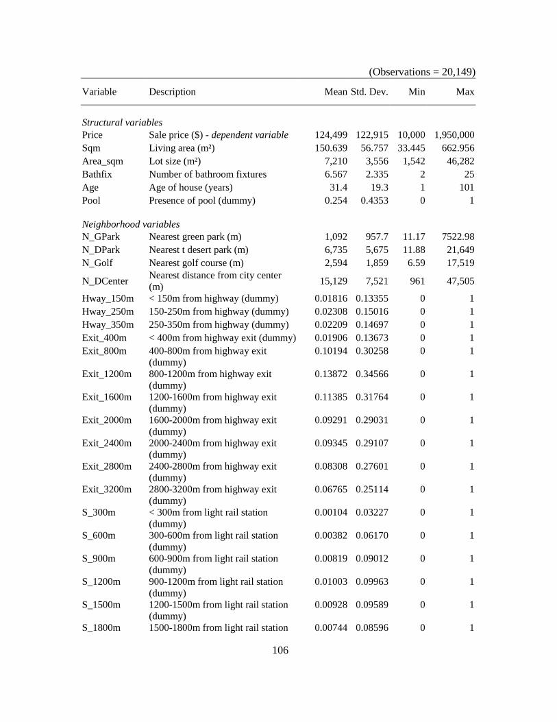
106

(Observations = 20,149)

Variable Description Mean Std. Dev. Min Max

Structural variables

Price Sale price ($) - dependent variable 124,499 122,915 10,000 1,950,000

Sqm Living area (m²) 150.639 56.757 33.445 662.956

Area_sqm Lot size (m²) 7,210 3,556 1,542 46,282

Bathfix Number of bathroom fixtures 6.567 2.335 2 25

Age Age of house (years) 31.4 19.3 1 101

Pool Presence of pool (dummy) 0.254 0.4353 0 1

Neighborhood variables

N_GPark Nearest green park (m) 1,092 957.7 11.17 7522.98

N_DPark Nearest t desert park (m) 6,735 5,675 11.88 21,649

N_Golf Nearest golf course (m) 2,594 1,859 6.59 17,519

N_DCenter Nearest distance from city center

(m) 15,129 7,521 961 47,505

Hway_150m < 150m from highway (dummy) 0.01816 0.13355 0 1

Hway_250m 150-250m from highway (dummy) 0.02308 0.15016 0 1

Hway_350m 250-350m from highway (dummy) 0.02209 0.14697 0 1

Exit_400m < 400m from highway exit (dummy) 0.01906 0.13673 0 1

Exit_800m 400-800m from highway exit

(dummy)

0.10194 0.30258 0 1

Exit_1200m 800-1200m from highway exit

(dummy)

0.13872 0.34566 0 1

Exit_1600m 1200-1600m from highway exit

(dummy)

0.11385 0.31764 0 1

Exit_2000m 1600-2000m from highway exit

(dummy)

0.09291 0.29031 0 1

Exit_2400m 2000-2400m from highway exit

(dummy)

0.09345 0.29107 0 1

Exit_2800m 2400-2800m from highway exit

(dummy)

0.08308 0.27601 0 1

Exit_3200m 2800-3200m from highway exit

(dummy)

0.06765 0.25114 0 1

S_300m < 300m from light rail station

(dummy)

0.00104 0.03227 0 1

S_600m 300-600m from light rail station

(dummy)

0.00382 0.06170 0 1

S_900m 600-900m from light rail station

(dummy)

0.00819 0.09012 0 1

S_1200m 900-1200m from light rail station

(dummy)

0.01003 0.09963 0 1

S_1500m 1200-1500m from light rail station

(dummy)

0.00928 0.09589 0 1

S_1800m 1500-1800m from light rail station 0.00744 0.08596 0 1

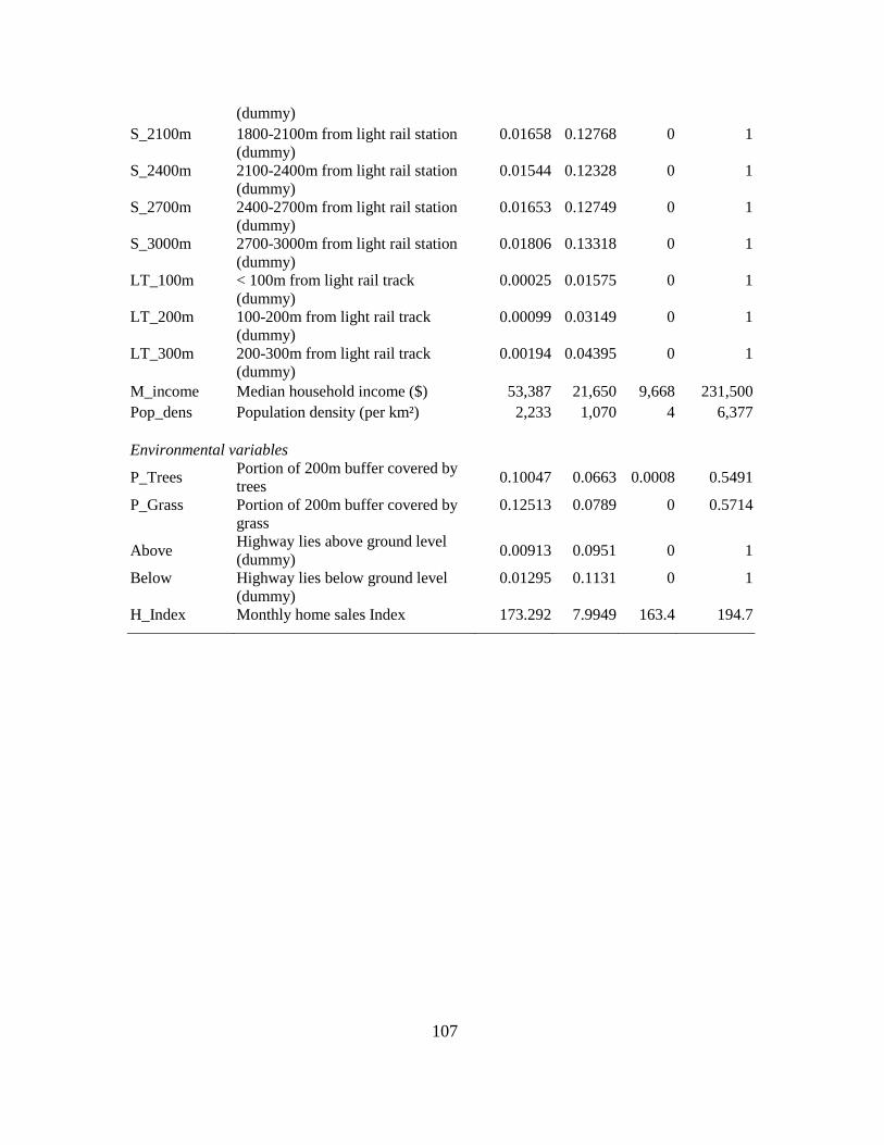
107

(dummy)

S_2100m 1800-2100m from light rail station

(dummy)

0.01658 0.12768 0 1

S_2400m 2100-2400m from light rail station

(dummy)

0.01544 0.12328 0 1

S_2700m 2400-2700m from light rail station

(dummy)

0.01653 0.12749 0 1

S_3000m 2700-3000m from light rail station

(dummy)

0.01806 0.13318 0 1

LT_100m < 100m from light rail track

(dummy)

0.00025 0.01575 0 1

LT_200m 100-200m from light rail track

(dummy)

0.00099 0.03149 0 1

LT_300m 200-300m from light rail track

(dummy)

0.00194 0.04395 0 1

M_income Median household income ($) 53,387 21,650 9,668 231,500

Pop_dens Population density (per km²) 2,233 1,070 4 6,377

Environmental variables

P_Trees Portion of 200m buffer covered by

trees 0.10047 0.0663 0.0008 0.5491

P_Grass Portion of 200m buffer covered by

grass

0.12513 0.0789 0 0.5714

Above Highway lies above ground level

(dummy) 0.00913 0.0951 0 1

Below Highway lies below ground level

(dummy)

0.01295 0.1131 0 1

H_Index Monthly home sales Index 173.292 7.9949 163.4 194.7

108

APPENDIX B

SUMMARY OF SELECTED LITERATURE ON ROAD AND RAIL IMPACTS IN

HEDONIC PRICE MODELS FOR COMMERCIAL PROPERTIES

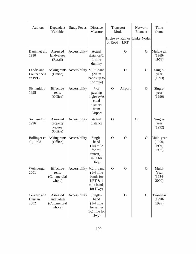
109

Authors Dependent

Variable

Study Focus Distance

Measure

Transport

Mode

Network

Element

Time

frame

Highway

or Road

Rail or

LRT

Links Nodes

Damm et al.,

1980

Assessed

landvalues

(Retail)

Accessibility Actual

distance/0.

1 mile

dummy

O O Multi-year

(1969-

1976)

Landis and

Loutzenheis

er 1995

Asking rents

(Office)

Accessibility Multi-band

(200m

bands up to

1/2 mile)

O O Single-

year

(1993)

Sivitanidou

1995

Effective

rents

(Office)

Accessibility # of

passing

highway/A

ctual

distance

from

Airport

O Airport O Single-

year

(1990)

Sivitanidou

1996

Assessed

property

values

(Office)

Accessibility Actual

distance

O O Single-

year

(1992)

Bollinger et

al., 1998

Asking rents

(Office)

Accessibility Single-

band

(1/4 mile

for rail

transit, 1

mile for

Hwy)

O O O Multi-year

(1990,

1994,

1996)

Weinberger

2001

Effective

rents

(Commercial

whole)

Accessibility Multi-band

(1/4 mile

bands for

LRT & 1

mile bands

for Hwy)

O O O Multi-

Year

(1984-

2000)

Cervero and

Duncan

2002

Assessed

land values

(Commercial

whole)

Accessibility Single-

band

(1/4 mile

for rail &

1/2 mile for

Hwy)

O O Two-year

(1998-

1999)

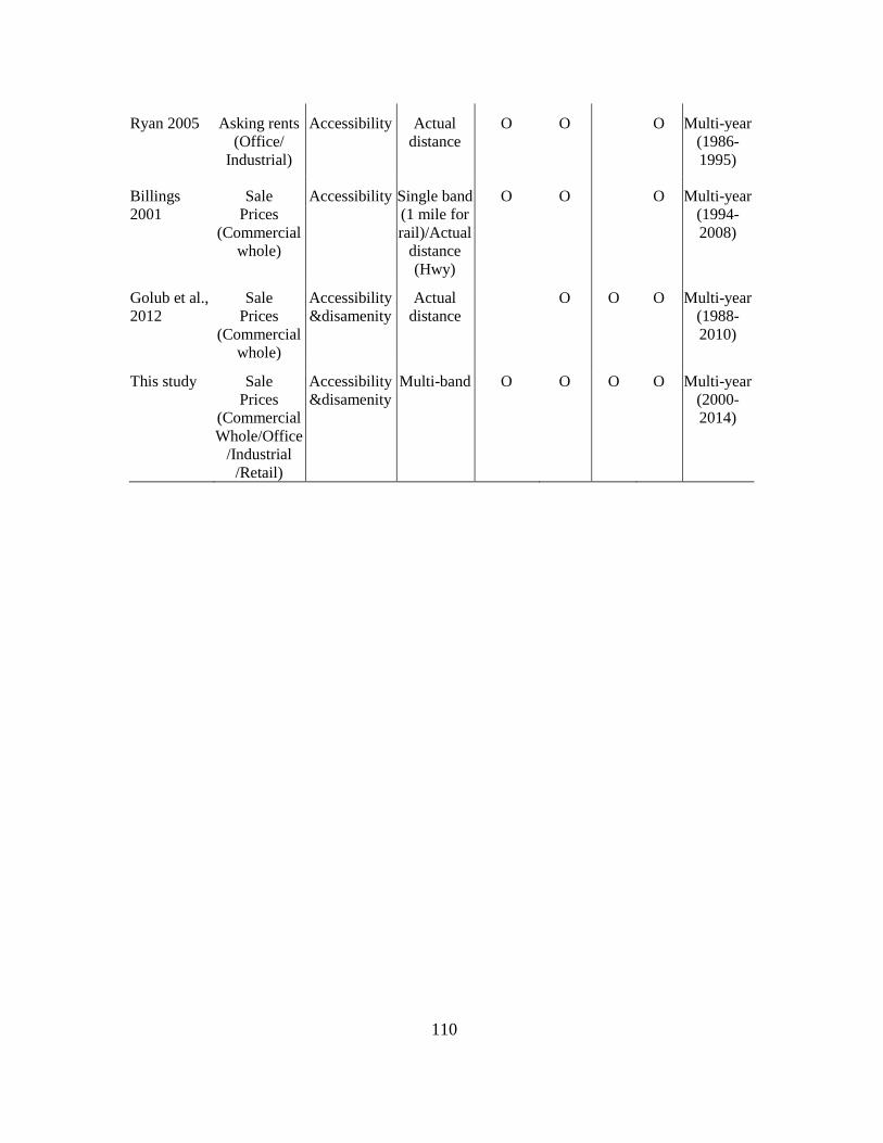
110

Ryan 2005 Asking rents

(Office/

Industrial)

Accessibility Actual

distance

O O O Multi-year

(1986-

1995)

Billings

2001

Sale

Prices

(Commercial

whole)

Accessibility Single band

(1 mile for

rail)/Actual

distance

(Hwy)

O O O Multi-year

(1994-

2008)

Golub et al.,

2012

Sale

Prices

(Commercial

whole)

Accessibility

&disamenity

Actual

distance

O O O Multi-year

(1988-

2010)

This study Sale

Prices

(Commercial

Whole/Office

/Industrial

/Retail)

Accessibility

&disamenity

Multi-band O O O O Multi-year

(2000-

2014)

111

APPENDIX C

ESTIMATION RESULTS FOR THE WHOLE COMMERCIAL PROPERTIES

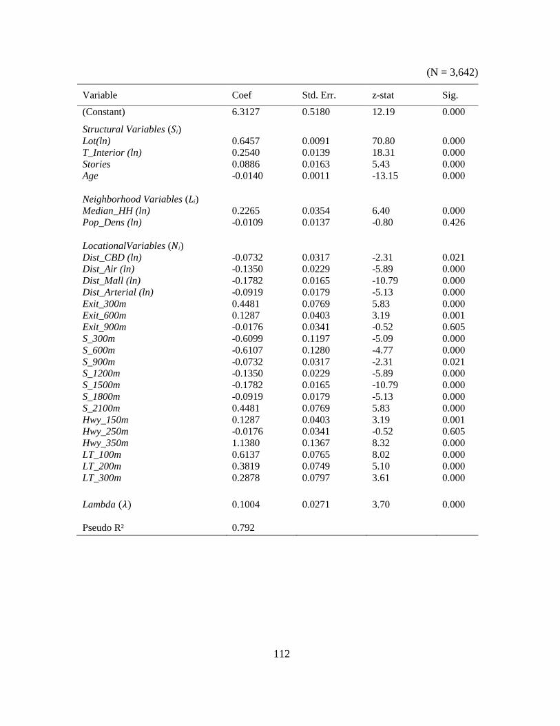
112

(N = 3,642)

Variable Coef Std. Err. z-stat Sig.

(Constant) 6.3127 0.5180 12.19 0.000

Structural Variables ( )

Lot(ln) 0.6457 0.0091 70.80 0.000

T_Interior (ln) 0.2540 0.0139 18.31 0.000

Stories 0.0886 0.0163 5.43 0.000

Age -0.0140 0.0011 -13.15 0.000

Neighborhood Variables ( )

Median_HH (ln) 0.2265 0.0354 6.40 0.000

Pop_Dens (ln) -0.0109 0.0137 -0.80 0.426

LocationalVariables ( )

Dist_CBD (ln) -0.0732 0.0317 -2.31 0.021

Dist_Air (ln) -0.1350 0.0229 -5.89 0.000

Dist_Mall (ln) -0.1782 0.0165 -10.79 0.000

Dist_Arterial (ln) -0.0919 0.0179 -5.13 0.000

Exit_300m 0.4481 0.0769 5.83 0.000

Exit_600m 0.1287 0.0403 3.19 0.001

Exit_900m -0.0176 0.0341 -0.52 0.605

S_300m -0.6099 0.1197 -5.09 0.000

S_600m -0.6107 0.1280 -4.77 0.000

S_900m -0.0732 0.0317 -2.31 0.021

S_1200m -0.1350 0.0229 -5.89 0.000

S_1500m -0.1782 0.0165 -10.79 0.000

S_1800m -0.0919 0.0179 -5.13 0.000

S_2100m 0.4481 0.0769 5.83 0.000

Hwy_150m 0.1287 0.0403 3.19 0.001

Hwy_250m -0.0176 0.0341 -0.52 0.605

Hwy_350m 1.1380 0.1367 8.32 0.000

LT_100m 0.6137 0.0765 8.02 0.000

LT_200m 0.3819 0.0749 5.10 0.000

LT_300m 0.2878 0.0797 3.61 0.000

Lambda 0.1004 0.0271 3.70 0.000

Pseudo R² 0.792

113

APPENDIX D

ESTIMATION RESULTS FOR THE INDUSTRIAL PROPERTIES

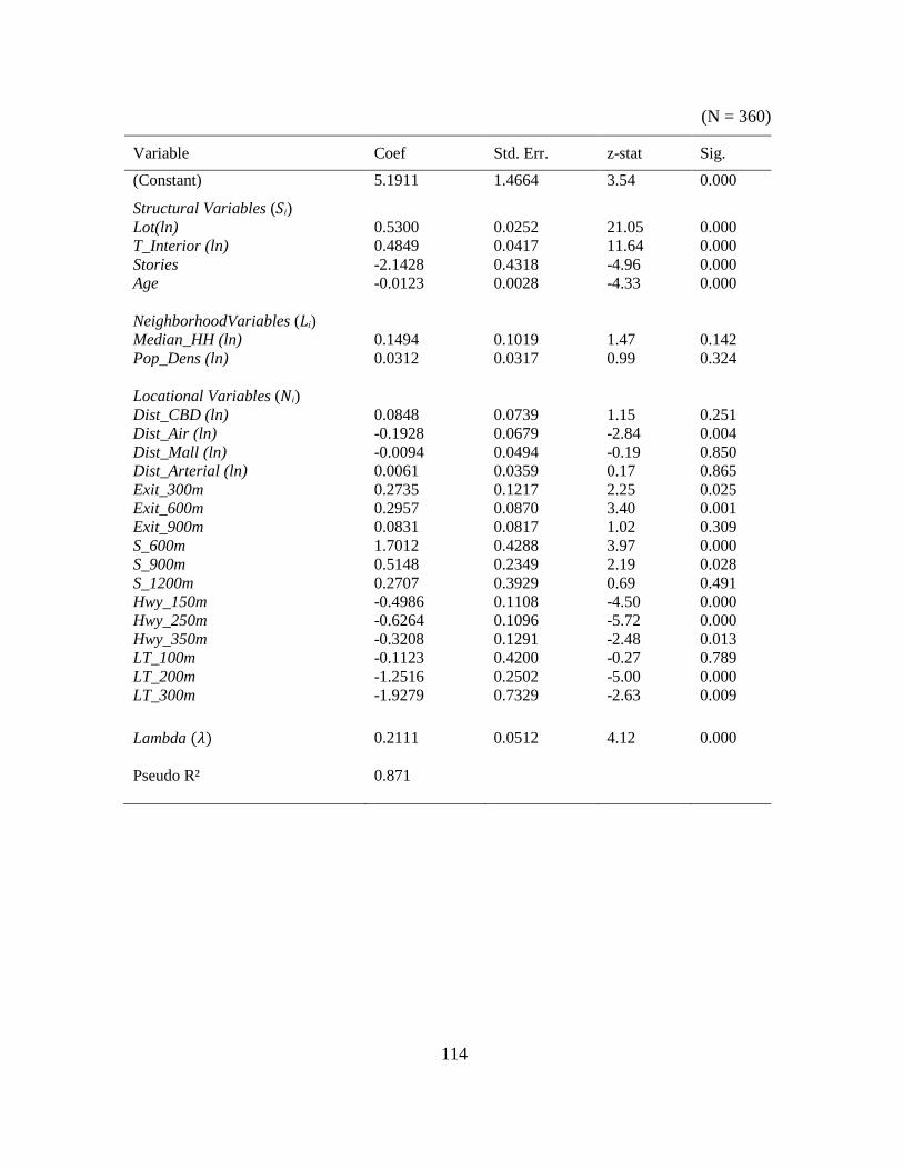
114

(N = 360)

Variable Coef Std. Err. z-stat Sig.

(Constant) 5.1911 1.4664 3.54 0.000

Structural Variables ( )

Lot(ln) 0.5300 0.0252 21.05 0.000

T_Interior (ln) 0.4849 0.0417 11.64 0.000

Stories -2.1428 0.4318 -4.96 0.000

Age -0.0123 0.0028 -4.33 0.000

NeighborhoodVariables ( )

Median_HH (ln) 0.1494 0.1019 1.47 0.142

Pop_Dens (ln) 0.0312 0.0317 0.99 0.324

Locational Variables ( )

Dist_CBD (ln) 0.0848 0.0739 1.15 0.251

Dist_Air (ln) -0.1928 0.0679 -2.84 0.004

Dist_Mall (ln) -0.0094 0.0494 -0.19 0.850

Dist_Arterial (ln) 0.0061 0.0359 0.17 0.865

Exit_300m 0.2735 0.1217 2.25 0.025

Exit_600m 0.2957 0.0870 3.40 0.001

Exit_900m 0.0831 0.0817 1.02 0.309

S_600m 1.7012 0.4288 3.97 0.000

S_900m 0.5148 0.2349 2.19 0.028

S_1200m 0.2707 0.3929 0.69 0.491

Hwy_150m -0.4986 0.1108 -4.50 0.000

Hwy_250m -0.6264 0.1096 -5.72 0.000

Hwy_350m -0.3208 0.1291 -2.48 0.013

LT_100m -0.1123 0.4200 -0.27 0.789

LT_200m -1.2516 0.2502 -5.00 0.000

LT_300m -1.9279 0.7329 -2.63 0.009

Lambda 0.2111 0.0512 4.12 0.000

Pseudo R² 0.871

115

APPENDIX E

ESTIMATION RESULTS FOR THE OFFICE PROPERTIES

116

(N = 1,214)

Variable Coef Std. Err. z-stat Sig.

(Constant) 7.4797 0.8121 9.21 0.000

Structural Variables ( )

Lot (ln) 0.5704 0.0155 36.79 0.000

T_Interior (ln) 0.3212 0.0254 12.66 0.000

Stories 0.0600 0.0178 3.36 0.001

Age -0.0131 0.0015 -8.50 0.000

Neighborhood Variables ( )

Median_HH (ln) 0.1715 0.0536 3.20 0.001

Pop_Dens (ln) 0.0248 0.0217 1.14 0.253

Locational Variables ( )

Dist_CBD (ln) -0.0678 0.0433 -1.57 0.117

Dist_Air (ln) -0.2253 0.0357 -6.32 0.000

Dist_Mall (ln) -0.2150 0.0280 -7.69 0.000

Dist_Arterial (ln) -0.0180 0.0226 -0.80 0.426

Exit_300m 0.4852 0.1272 3.82 0.000

Exit_600m 0.1026 0.0595 1.72 0.085

Exit_900m -0.0064 0.0482 -0.13 0.895

S_300m 0.7605 0.1704 4.46 0.000

S_600m 0.5427 0.0929 5.84 0.000

S_900m 0.2913 0.1121 2.60 0.009

S_1200m 0.4369 0.1222 3.58 0.000

S_1500m 0.1974 0.1559 1.27 0.205

Hwy_150m -0.1386 0.1290 -1.07 0.283

Hwy_250m 0.0703 0.1121 0.63 0.530

Hwy_350m 0.0425 0.0879 0.48 0.628

LT_100m -0.4832 0.1469 -3.29 0.001

LT_200m -0.1370 0.1829 -0.75 0.454

LT_300m -0.4380 0.1452 -3.02 0.003

Lambda 0.2197 0.0388 5.66 0.000

Pseudo R² 0.83

117

APPENDIX F

ESTIMATION RESULTS FOR RETAIL AND SERVICE PROPERTIES

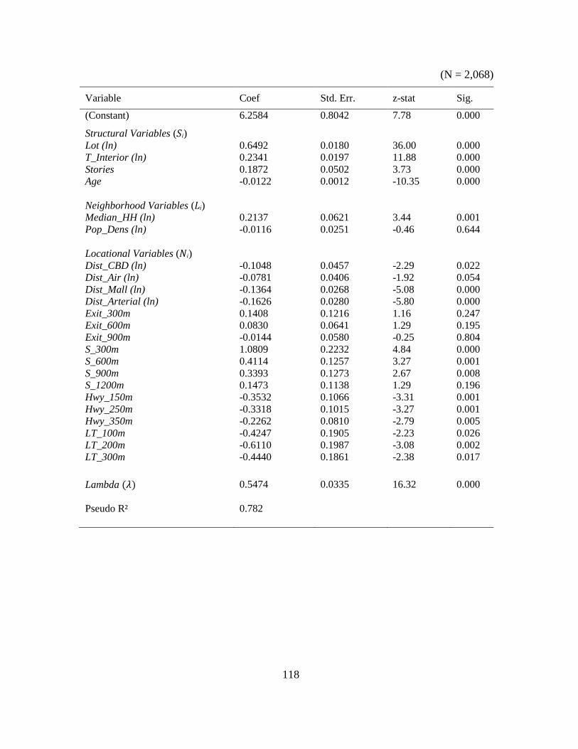
118

(N = 2,068)

Variable Coef Std. Err. z-stat Sig.

(Constant) 6.2584 0.8042 7.78 0.000

Structural Variables ( )

Lot (ln) 0.6492 0.0180 36.00 0.000

T_Interior (ln) 0.2341 0.0197 11.88 0.000

Stories 0.1872 0.0502 3.73 0.000

Age -0.0122 0.0012 -10.35 0.000

Neighborhood Variables ( )

Median_HH (ln) 0.2137 0.0621 3.44 0.001

Pop_Dens (ln) -0.0116 0.0251 -0.46 0.644

Locational Variables ( )

Dist_CBD (ln) -0.1048 0.0457 -2.29 0.022

Dist_Air (ln) -0.0781 0.0406 -1.92 0.054

Dist_Mall (ln) -0.1364 0.0268 -5.08 0.000

Dist_Arterial (ln) -0.1626 0.0280 -5.80 0.000

Exit_300m 0.1408 0.1216 1.16 0.247

Exit_600m 0.0830 0.0641 1.29 0.195

Exit_900m -0.0144 0.0580 -0.25 0.804

S_300m 1.0809 0.2232 4.84 0.000

S_600m 0.4114 0.1257 3.27 0.001

S_900m 0.3393 0.1273 2.67 0.008

S_1200m 0.1473 0.1138 1.29 0.196

Hwy_150m -0.3532 0.1066 -3.31 0.001

Hwy_250m -0.3318 0.1015 -3.27 0.001

Hwy_350m -0.2262 0.0810 -2.79 0.005

LT_100m -0.4247 0.1905 -2.23 0.026

LT_200m -0.6110 0.1987 -3.08 0.002

LT_300m -0.4440 0.1861 -2.38 0.017

Lambda 0.5474 0.0335 16.32 0.000

Pseudo R² 0.782

119

APPENDIX G

DETAILED RESULTS FOR VALLEJO

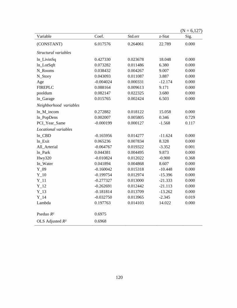
120

(N = 6,127)

Variable Coef. Std.err z-Stat Sig.

(CONSTANT) 6.017576 0.264061 22.789 0.000

Structural variables

ln_LivinSq 0.427330 0.023678 18.048 0.000

ln_LotSqft 0.073282 0.011486 6.380 0.000

N_Rooms 0.038432 0.004267 9.007 0.000

N_Story 0.043093 0.011087 3.887 0.000

Age -0.004024 0.000331 -12.174 0.000

FIREPLC 0.088164 0.009613 9.171 0.000

pooldum 0.082147 0.022325 3.680 0.000

ln_Garage 0.015765 0.002424 6.503 0.000

Neighborhood variables

ln_M_incom 0.272882 0.018122 15.058 0.000

ln_PopDens 0.002007 0.005805 0.346 0.729

PCI_Year_Same -0.000199 0.000127 -1.568 0.117

Locational variables

ln_CBD -0.165956 0.014277 -11.624 0.000

ln_Exit 0.065236 0.007834 8.328 0.000

All_Arterial -0.064767 0.019322 -3.352 0.001

ln_Park 0.044381 0.004495 9.873 0.000

Hwy320 -0.010824 0.012022 -0.900 0.368

In_Water 0.041894 0.004868 8.607 0.000

Y_09 -0.160042 0.015318 -10.448 0.000

Y_10 -0.199754 0.012974 -15.396 0.000

Y_11 -0.277327 0.013000 -21.333 0.000

Y_12 -0.262691 0.012442 -21.113 0.000

Y_13 -0.181814 0.013709 -13.262 0.000

Y_14 -0.032750 0.013965 -2.345 0.019

Lambda 0.197763 0.014103 14.022 0.000

Pseduo R² 0.6975

OLS Adjusted R² 0.6968

121

APPENDIX H

DETAILED RESULTS FOR VACAVILLE

122

(N = 5,165)

Variable Coef. Std.err z-Stat Sig.

(CONSTANT) 7.323418 0.192834 37.978 0.000

Structural variables

ln_LivinSq 0.592843 0.019064 31.097 0.000

ln_LotSqft 0.139476 0.010687 13.051 0.000

N_Rooms 0.002322 0.003805 0.610 0.542

N_Story -0.031342 0.006297 -4.977 0.000

Age -0.006558 0.000351 -18.679 0.000

FIREPLC 0.028646 0.007788 3.678 0.000

pooldum 0.070016 0.006079 11.517 0.000

ln_Garage 0.004628 0.003618 1.279 0.201

Neighborhood variables

ln_M_incom 0.053484 0.015073 3.548 0.000

ln_PopDens -0.032788 0.003319 -9.880 0.000

PCI_Year_Same -0.000135 0.000173 -0.781 0.435

Locational variables

ln_CBD -0.069189 0.008111 -8.530 0.000

ln_Exit 0.027390 0.006860 3.993 0.000

All_Arterial -0.021555 0.017183 -1.254 0.210

ln_Park -0.001989 0.002515 -0.791 0.429

Hwy320 -0.081328 0.023540 -3.455 0.001

Y_09 0.068406 0.009486 7.211 0.000

Y_10 0.003586 0.007541 0.476 0.634

Y_11 -0.044223 0.008097 -5.461 0.000

Y_12 -0.051043 0.007302 -6.990 0.000

Y_13 -0.010513 0.008366 -1.257 0.209

Y_14 0.040298 0.007075 5.696 0.000

Lambda 0.213770 0.015327 13.947 0.000

Pseduo R² 0.7742

OLS Adjusted R² 0.7734

123

APPENDIX I

DETAILED RESULTS FOR FAIRFIELD

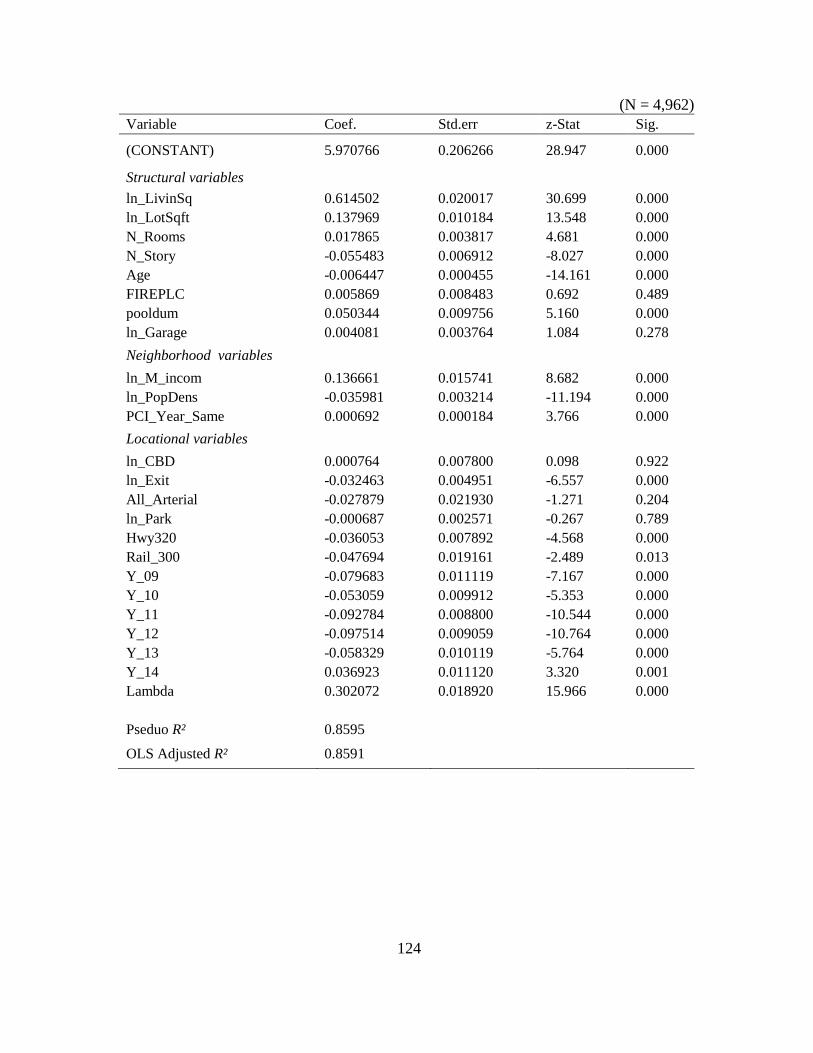
124

(N = 4,962)

Variable Coef. Std.err z-Stat Sig.

(CONSTANT) 5.970766 0.206266 28.947 0.000

Structural variables

ln_LivinSq 0.614502 0.020017 30.699 0.000

ln_LotSqft 0.137969 0.010184 13.548 0.000

N_Rooms 0.017865 0.003817 4.681 0.000

N_Story -0.055483 0.006912 -8.027 0.000

Age -0.006447 0.000455 -14.161 0.000

FIREPLC 0.005869 0.008483 0.692 0.489

pooldum 0.050344 0.009756 5.160 0.000

ln_Garage 0.004081 0.003764 1.084 0.278

Neighborhood variables

ln_M_incom 0.136661 0.015741 8.682 0.000

ln_PopDens -0.035981 0.003214 -11.194 0.000

PCI_Year_Same 0.000692 0.000184 3.766 0.000

Locational variables

ln_CBD 0.000764 0.007800 0.098 0.922

ln_Exit -0.032463 0.004951 -6.557 0.000

All_Arterial -0.027879 0.021930 -1.271 0.204

ln_Park -0.000687 0.002571 -0.267 0.789

Hwy320 -0.036053 0.007892 -4.568 0.000

Rail_300 -0.047694 0.019161 -2.489 0.013

Y_09 -0.079683 0.011119 -7.167 0.000

Y_10 -0.053059 0.009912 -5.353 0.000

Y_11 -0.092784 0.008800 -10.544 0.000

Y_12 -0.097514 0.009059 -10.764 0.000

Y_13 -0.058329 0.010119 -5.764 0.000

Y_14 0.036923 0.011120 3.320 0.001

Lambda 0.302072 0.018920 15.966 0.000

Pseduo R² 0.8595

OLS Adjusted R² 0.8591

125

APPENDIX J

DETAILED RESULTS FOR SUISUN CITY

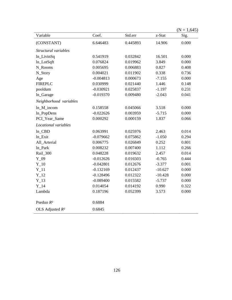
126

(N = 1,645)

Variable Coef. Std.err z-Stat Sig.

(CONSTANT) 6.646483 0.445893 14.906 0.000

Structural variables

ln_LivinSq 0.541919 0.032842 16.501 0.000

ln_LotSqft 0.076824 0.019962 3.849 0.000

N_Rooms 0.005695 0.006883 0.827 0.408

N_Story 0.004021 0.011902 0.338 0.736

Age -0.004813 0.000673 -7.155 0.000

FIREPLC 0.030999 0.021440 1.446 0.148

pooldum -0.030921 0.025837 -1.197 0.231

ln_Garage -0.019370 0.009480 -2.043 0.041

Neighborhood variables

ln_M_incom 0.158558 0.045066 3.518 0.000

ln_PopDens -0.022626 0.003959 -5.715 0.000

PCI_Year_Same 0.000292 0.000159 1.837 0.066

Locational variables

ln_CBD 0.063991 0.025976 2.463 0.014

ln_Exit -0.079662 0.075862 -1.050 0.294

All_Arterial 0.006775 0.026849 0.252 0.801

ln_Park 0.008232 0.007400 1.112 0.266

Rail_300 0.048228 0.019632 2.457 0.014

Y_09 -0.012626 0.016503 -0.765 0.444

Y_10 -0.042801 0.012676 -3.377 0.001

Y_11 -0.132169 0.012437 -10.627 0.000

Y_12 -0.128496 0.012322 -10.428 0.000

Y_13 -0.089400 0.015582 -5.737 0.000

Y_14 0.014054 0.014192 0.990 0.322

Lambda 0.187196 0.052399 3.573 0.000

Pseduo R² 0.6884

OLS Adjusted R² 0.6845

127

APPENDIX K

DETAILED RESULTS FOR BENICIA

128

(N = 971)

Variable Coef. Std.err z-Stat Sig.

(CONSTANT) 9.677788 0.394037 24.561 0.000

Structural variables

ln_LivinSq 0.370596 0.032714 11.328 0.000

ln_LotSqft 0.130883 0.019022 6.881 0.000

N_Rooms 0.031007 0.006182 5.016 0.000

N_Story -0.033080 0.012277 -2.695 0.007

Age -0.002529 0.000778 -3.251 0.001

FIREPLC 0.030715 0.017734 1.732 0.084

pooldum 0.036694 0.021116 1.738 0.083

ln_Garage 0.012369 0.005299 2.334 0.020

Neighborhood variables

ln_M_incom -0.017523 0.034474 -0.508 0.611

ln_PopDens 0.027344 0.006047 4.522 0.000

PCI_Year_Same -0.000409 0.000242 -1.689 0.091

Locational variables

ln_CBD -0.073841 0.017193 -4.295 0.000

ln_Exit 0.048054 0.016273 2.953 0.003

All_Arterial 0.569833 0.155511 3.664 0.000

ln_Park 0.005921 0.005772 1.026 0.305

Hwy320 -0.067580 0.021376 -3.162 0.002

ln_Water -0.052992 0.008896 -5.957 0.000

Y_09 0.152637 0.022313 6.841 0.000

Y_10 0.059731 0.018831 3.172 0.002

Y_11 0.012265 0.017994 0.682 0.496

Y_12 0.007036 0.017623 0.399 0.690

Y_13 0.003733 0.018209 0.205 0.838

Y_14 0.012183 0.020224 0.602 0.547

OLS Adjusted R² 0.7453

129

APPENDIX L

DETAILED RESULTS FOR DIXON

130

(N = 279)

Variable Coef. Std.err z-Stat Sig.

(CONSTANT) 8.420707 1.192911 7.059 0.000

Structural variables

ln_LivinSq 0.452588 0.049480 9.147 0.000

ln_LotSqft 0.112033 0.029315 3.822 0.000

N_Rooms -0.002657 0.009707 -0.274 0.785

N_Story -0.000344 0.017246 -0.020 0.984

Age 0.000324 0.000888 0.365 0.715

FIREPLC 0.158933 0.029164 5.450 0.000

pooldum 0.033420 0.020374 1.640 0.102

ln_Garage 0.007918 0.014536 0.545 0.586

Neighborhood variables

ln_M_incom -0.234321 0.089847 -2.608 0.010

ln_PopDens -0.059096 0.019751 -2.992 0.003

PCI_Year_Same -0.003663 0.000678 -5.404 0.000

Locational variables

ln_CBD 0.348714 0.048736 7.155 0.000

ln_Exit 0.076687 0.028198 2.720 0.007

ln_Park 0.003750 0.009479 0.396 0.693

Hwy320 0.010192 0.019681 0.518 0.605

Y_09 0.144242 0.028864 4.997 0.000

Y_10 0.083654 0.026488 3.158 0.002

Y_11 0.018345 0.025816 0.711 0.478

Y_12 0.025416 0.026028 0.976 0.330

Y_13 0.031182 0.027046 1.153 0.250

Y_14 0.065733 0.026933 2.441 0.015

OLS Adjusted R² 0.8149

131

APPENDIX M

DETAILED RESULTS FOR RIO VISTA

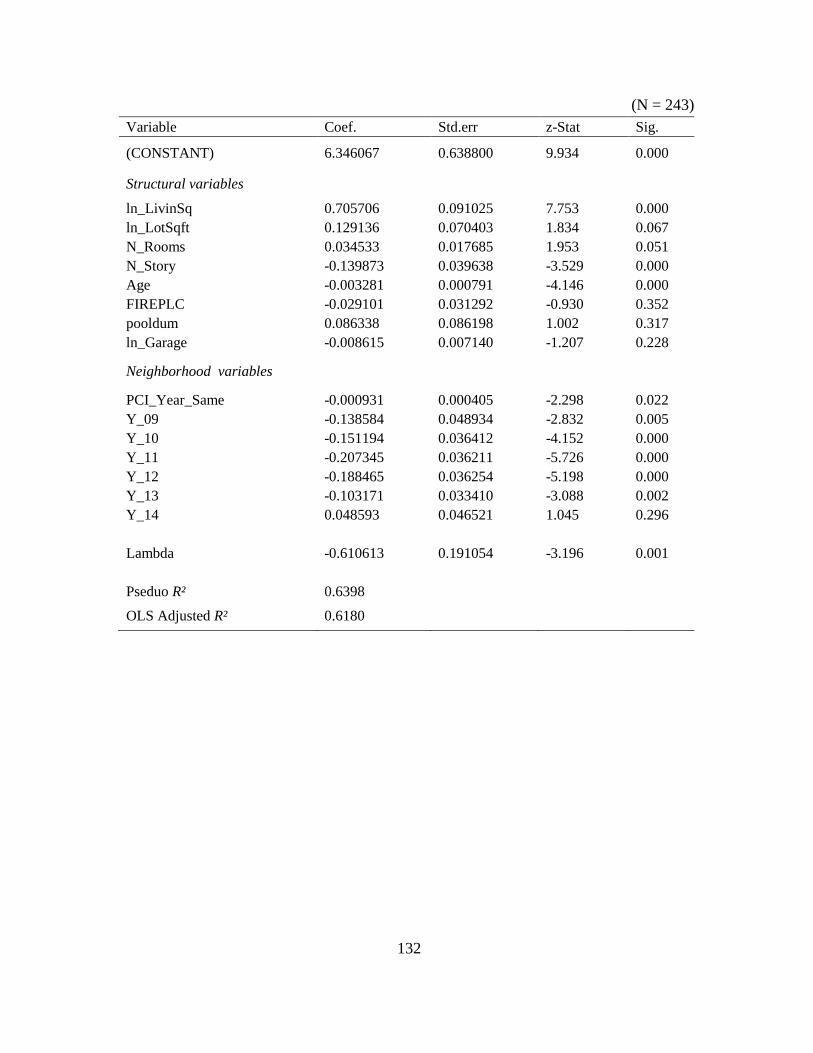
132

(N = 243)

Variable Coef. Std.err z-Stat Sig.

(CONSTANT) 6.346067 0.638800 9.934 0.000

Structural variables

ln_LivinSq 0.705706 0.091025 7.753 0.000

ln_LotSqft 0.129136 0.070403 1.834 0.067

N_Rooms 0.034533 0.017685 1.953 0.051

N_Story -0.139873 0.039638 -3.529 0.000

Age -0.003281 0.000791 -4.146 0.000

FIREPLC -0.029101 0.031292 -0.930 0.352

pooldum 0.086338 0.086198 1.002 0.317

ln_Garage -0.008615 0.007140 -1.207 0.228

Neighborhood variables

PCI_Year_Same -0.000931 0.000405 -2.298 0.022

Y_09 -0.138584 0.048934 -2.832 0.005

Y_10 -0.151194 0.036412 -4.152 0.000

Y_11 -0.207345 0.036211 -5.726 0.000

Y_12 -0.188465 0.036254 -5.198 0.000

Y_13 -0.103171 0.033410 -3.088 0.002

Y_14 0.048593 0.046521 1.045 0.296

Lambda -0.610613 0.191054 -3.196 0.001

Pseduo R² 0.6398

OLS Adjusted R² 0.6180

133

APPENDIX N

DETAILED RESULTS FOR SOLANO COUNTY

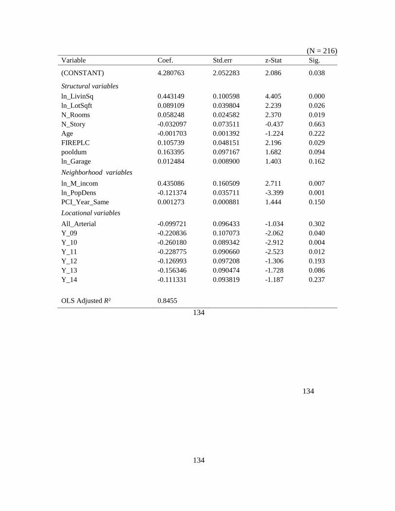
134

(N = 216)

Variable Coef. Std.err z-Stat Sig.

(CONSTANT) 4.280763 2.052283 2.086 0.038

Structural variables

ln_LivinSq 0.443149 0.100598 4.405 0.000

ln_LotSqft 0.089109 0.039804 2.239 0.026

N_Rooms 0.058248 0.024582 2.370 0.019

N_Story -0.032097 0.073511 -0.437 0.663

Age -0.001703 0.001392 -1.224 0.222

FIREPLC 0.105739 0.048151 2.196 0.029

pooldum 0.163395 0.097167 1.682 0.094

ln_Garage 0.012484 0.008900 1.403 0.162

Neighborhood variables

ln_M_incom 0.435086 0.160509 2.711 0.007

ln_PopDens -0.121374 0.035711 -3.399 0.001

PCI_Year_Same 0.001273 0.000881 1.444 0.150

Locational variables

All_Arterial -0.099721 0.096433 -1.034 0.302

Y_09 -0.220836 0.107073 -2.062 0.040

Y_10 -0.260180 0.089342 -2.912 0.004

Y_11 -0.228775 0.090660 -2.523 0.012

Y_12 -0.126993 0.097208 -1.306 0.193

Y_13 -0.156346 0.090474 -1.728 0.086

Y_14 -0.111331 0.093819 -1.187 0.237

OLS Adjusted R² 0.8455

134

134