Impacts of Population and Income Growth Rates on ... · Impacts of Population and Income Growth...

Impacts of Population and Income Growth Rates

on Threatened Mammals and Birds

Ram Pandit

Corresponding author

School of Agricultural and Resource Economics,

Faculty of Sciences,

University of Western Australia

35 Stirling Highway

Crawley, WA 6009, Australia

Phone: +61 8 6488 1353

Fax: 61 8 6488 1098

email: [email protected]

David N Laband

School of Economics

Ivan Allen College of Liberal Arts

Georgia Institute of Technology

221 Bobby Dodd Way

Atlanta, GA 30332, USA

email: [email protected]

mailto:[email protected]

mailto:[email protected]



Abstract

Per capita income and human population levels have direct influences on environmental

outcomes of a country. Countries with same level of income (population size) may have a

different rate of income (population) growth and vice versa, suggesting that the influence of

the rate of income (population) growth on environmental outcomes could be different than

that of income (population) level. We explore this empirical question using country-level

data on threatened species published by International Union for Conservation of Nature for

the year 2007. Controlling for other factors, including spatial dependency among countries,

our model estimates the influences of the rate of income and population growth on threatened

mammals and birds across 113 continental countries. The results suggest that, among other

factors, the rate of population growth has a significant influence on number of threatened

birds in a country.

Keywords: Income growth rate, Population growth rate, Spatial autocorrelation, Endemic

species, Threatened species

JEL Codes: Q56, Q57

Please do not cite or quote without permission of authors. All errors remain the

responsibility of the authors.

1



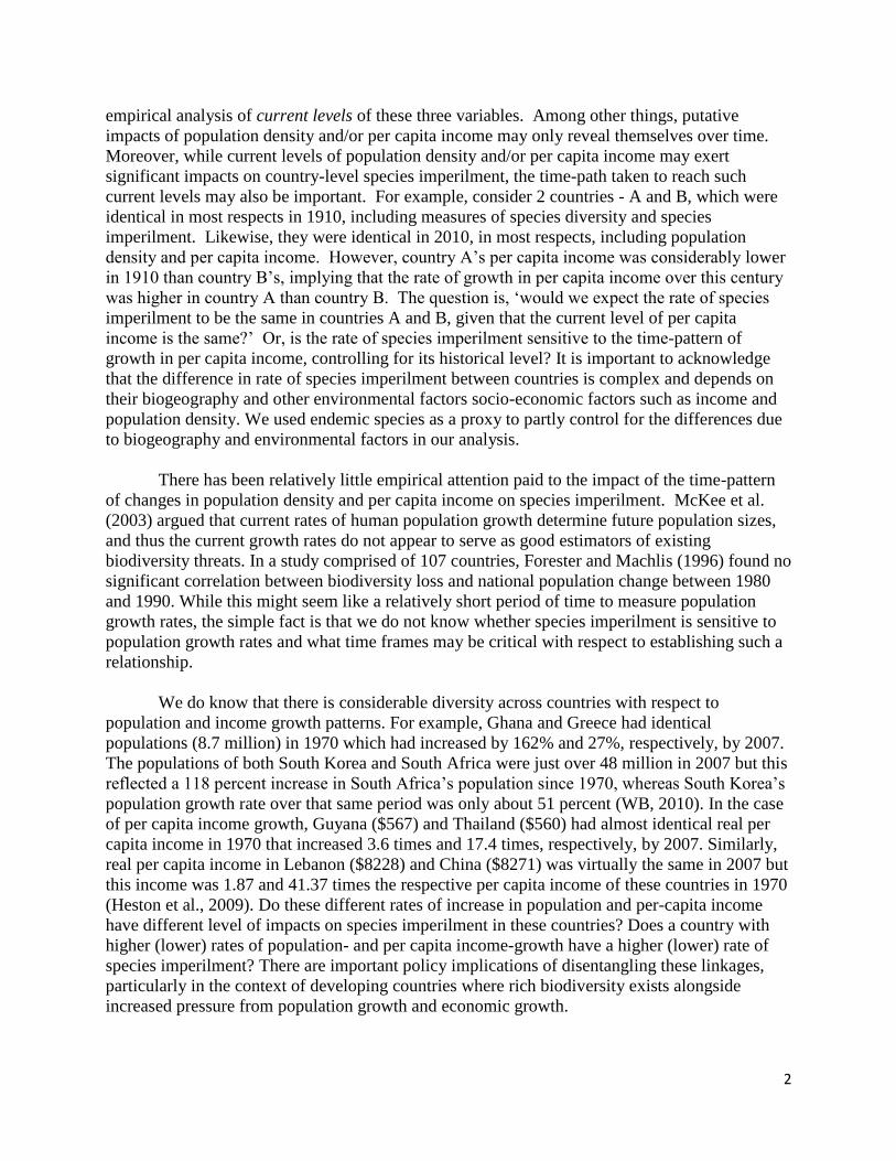
1. Introduction

Accelerated biodiversity loss is one of the serious environmental challenges faced by the

society today. Evidence indicates that, among a number of taxa groups, we are experiencing one

of the worst episodes of mass extinction of species since dinosaurs roamed the earth 65 million

years ago (CI, 2010; Hoffmann et al., 2010). In the past four decades (1970 to 2010), the sheer

number of threatened species has grown dramatically, exceeding the normal background rate of

extinction by a factor of two to three; and forecast scenarios for the 21st century consistently

indicate that biodiversity will continue to decline (Pereira et al., 2010). A general consensus

among scientists and policy makers is that both changes in natural habitat conditions and human

activities are responsible for this extinction crisis (Balmford and Bond, 2005; Forester and

Machlis, 1996; Kerr and Currie, 1995; Pereira et al., 2010; Sala et al., 2000). In addition, recent

studies examining causal relationship between specific drivers and biodiversity loss highlighted

five direct (i.e. habitat change, overexploitation, pollution, invasive alien species and climate

change) and several indirect (i.e. demographic change, economic activity, levels of international

trade, per capita consumption patterns, cultural and religious factors, and scientific and

technological changes) drivers of biodiversity loss (NBL, 2010; SCBD, 2010; TEEB, 2010). To

address these drivers, international agreements - such as Convention on Biological Diversity -

have stressed the need to effectively tackle the indirect drivers of biodiversity loss to achieve

global conservation goals, such as Aichi Biodiversity Targets (CI, 2010).

Both natural and anthropogenic pressure on the Earth’s biodiversity is reflected by

threatened species of flora and fauna (Dietz and Adger, 2003). The number of threatened species

also serves as an important indicator of ecological impacts of direct and indirect drivers of

biodiversity loss. Among indirect drivers, human population (population density) and economic

activity (level of per-capita income) are the two most widely studied drivers of threatened

species (Sodhi et al., 2008). In a cross-country context, human population density and per-capita

income in a given year have been shown to influence the number (or percentage) of threatened

species listed in International Union for Conservation of Nature (IUCN) Red Lists in that year

(Asafu-Adjaye, 2003; Naidoo and Adamowicz, 2001; Pandit and Laband, 2007a). While the

relationship between per-capita income and threatened species has been characterized by an

Environmental Kuznets Curve (EKC) for some taxa, this relationship is not universal across taxa

and studies. The relationship depends on several factors including the number of sample

countries and functional forms used in the analysis (McPherson and Nieswiadomy, 2005; Naidoo

and Adamowicz, 2001; Pandit and Laband, 2007b; Zibaei and Sheykh, 2009). Additionally, both

McPherson and Nieswiadomy (2005) and Pandit and Laband (2007b) have demonstrated the

importance of cross-border (or spatial) effects and its impact on empirical estimates of factors

influencing species imperilment drawn from cross-section models.

These studies employed cross-section data to predict the impact of population density and per-

capita income on either the number or percentage of threatened species of specific taxa. But the

relationship between human population density and species imperilment and the relationship

between per capita income and species imperilment may be more complex than suggested by an

2

empirical analysis of current levels of these three variables. Among other things, putative

impacts of population density and/or per capita income may only reveal themselves over time.

Moreover, while current levels of population density and/or per capita income may exert

significant impacts on country-level species imperilment, the time-path taken to reach such

current levels may also be important. For example, consider 2 countries - A and B, which were

identical in most respects in 1910, including measures of species diversity and species

imperilment. Likewise, they were identical in 2010, in most respects, including population

density and per capita income. However, country A’s per capita income was considerably lower

in 1910 than country B’s, implying that the rate of growth in per capita income over this century

was higher in country A than country B. The question is, ‘would we expect the rate of species

imperilment to be the same in countries A and B, given that the current level of per capita

income is the same?’ Or, is the rate of species imperilment sensitive to the time-pattern of

growth in per capita income, controlling for its historical level? It is important to acknowledge

that the difference in rate of species imperilment between countries is complex and depends on

their biogeography and other environmental factors socio-economic factors such as income and

population density. We used endemic species as a proxy to partly control for the differences due

to biogeography and environmental factors in our analysis.

There has been relatively little empirical attention paid to the impact of the time-pattern

of changes in population density and per capita income on species imperilment. McKee et al.

(2003) argued that current rates of human population growth determine future population sizes,

and thus the current growth rates do not appear to serve as good estimators of existing

biodiversity threats. In a study comprised of 107 countries, Forester and Machlis (1996) found no

significant correlation between biodiversity loss and national population change between 1980

and 1990. While this might seem like a relatively short period of time to measure population

growth rates, the simple fact is that we do not know whether species imperilment is sensitive to

population growth rates and what time frames may be critical with respect to establishing such a

relationship.

We do know that there is considerable diversity across countries with respect to

population and income growth patterns. For example, Ghana and Greece had identical

populations (8.7 million) in 1970 which had increased by 162% and 27%, respectively, by 2007.

The populations of both South Korea and South Africa were just over 48 million in 2007 but this

reflected a 118 percent increase in South Africa’s population since 1970, whereas South Korea’s

population growth rate over that same period was only about 51 percent (WB, 2010). In the case

of per capita income growth, Guyana ($567) and Thailand ($560) had almost identical real per

capita income in 1970 that increased 3.6 times and 17.4 times, respectively, by 2007. Similarly,

real per capita income in Lebanon ($8228) and China ($8271) was virtually the same in 2007 but

this income was 1.87 and 41.37 times the respective per capita income of these countries in 1970

(Heston et al., 2009). Do these different rates of increase in population and per-capita income

have different level of impacts on species imperilment in these countries? Does a country with

higher (lower) rates of population- and per capita income-growth have a higher (lower) rate of

species imperilment? There are important policy implications of disentangling these linkages,

particularly in the context of developing countries where rich biodiversity exists alongside

increased pressure from population growth and economic growth.

3

We tend to agree with McKee et al. (2003) who argue that there should be a lagged or

temporal effect of these drivers on threatened species. For example, among other drivers, the

threatened status of mammals in a country in 2007 could have been the result of economic

activities and population growth during earlier decades. Because of the difficulties in obtaining

statistically sufficient longitudinal data, empirical researchers examining factors that influence

species imperilment have tended to use cross-sectional data, (substituting space for time). A few

recent studies have considered a specific time in the past to examine the lagged effects (e.g.,

Mikkelson et al., 2007; Pandit and Laband, 2009) but they differ with respect to modelling and

estimation techniques. In this paper we explore whether species imperilment is statistically

sensitive to long-term impacts of population growth and economic activity by examining the

relationship between the average rates of population and per-capita income growth from 1970-

1990 and the number of threatened mammals and birds listed in IUCN’s Red List in 2007 among

113 non-island countries. In what follows, we describe our models - including the model to

control for spatial effects - data and methods in section 2, estimation results and discussion in

sections 3 and 4, and concluding remarks in section 5.

2. Model, Data, and Methods

2.1. Model

We posit a taxa-specific reduced form model from the conceptual model presented in Eq.

1 to investigate country specific impacts of the rate of population and per-capita income growth

on the number of threatened mammals and birds. The conceptual model can be expressed as

Threatened species = f (total species, endemic species, land area, human population density,

gross national income, rates of population and income growth) (Eq. 1)

The reduced form model in Eq. 2 links the number of threatened mammals and birds in a country

with hypothesized determinants (X matrix) represented by the model as ' ij ij ijy x , i=

countries (1 to 113), j = taxa (1 for mammal and 2 for bird). In a matrix form, the model is

y X ε (Eq. 2)

where y is an n x 1 vector of independent variable (number of threatened species – mammals or

birds); X is a n x k matrix of explanatory variables that include number of endemic species,

country area, population density, per capita income, population growth rate, and income growth

rate; β is a k x 1 vector of regression coefficients; and ε is the n x 1 vector of error terms.

The number of threatened species refers to the number of critically endangered, endangered, and

vulnerable species of mammals and birds for 113 countries, as listed in the 2007 IUCN Red Lists

of Threatened Species (IUCN, 2007). We included land area, human population density and per

capita income levels as predictor variables in the model to control for the effect of available

space for all species as well as human-induced pressure on other species by virtue of sheer

population size relative to area and economic activities. Earlier studies have indicated that the

number of endemic species, species with limited distributional range, in a country is a significant

predictor of the number of threatened/endangered species (McKee et al., 2003; Pandit and

Laband, 2007a). We include this variable in the model, but we do not include the total number of

4

species as a predictor variable due to significantly high correlation (p > 0.001) between endemic

and total number of species for the taxa we analysed.

A priori, we expect that the number of endemic species in a country, the human population

density, and the per capita income will be positively related to the number of threatened species

of mammals and birds in that country. Further, we expect that, controlling for historical

population density and per capita income levels, the rate of population and per-capita income

growth in earlier periods will be related positively to the number of threatened species in a later

period.

We consider population and per capita income growth rates from 1970 to 1990 to capture the

temporal effect of these variables on the number of threatened mammals and birds in 2007. The

use 1970 as a base year for the analysis is partly because this pushes the limit on how far back in

time we can go while still guaranteeing availability of satisfactory data on key model variables

for a large number of countries and the emergence of environmental conservation movement in

different parts of the world (e.g. establishment of national environmental protection agencies in a

number of countries, including the United States). The use of year 1990 is to allow some time lag

to reflect the effect of these variables on number of threatened species in 2007 and also to

coincide roughly with the first Earth Summit (5 June 1992) that opened the Convention on

Biological Diversity for signature among parties which came to effect on 29 December 1993.

To capture the spatial effects or spill-over effects on species imperilment from neighbouring

observations, the model in Eq. 2 is further modified based on the nature and the significance of

spatial dependency among observations. If y (number of threatened species) is endogenously

determined, i.e. the threatened species in a country depends on the number of threatened species

in neighbouring countries, then the Eq. 2 takes a form of spatial lag model (Eq. 3) that captures

the spatial effect in the model by augmenting lagged value of independent variable (Wy) as a

predictor, where W is a spatial weight matrix based on a particular type of spatial dependency

(e.g. simple binary contiguity or inverse distance) among observations and ρ is the spatial lag

parameter. If the errors among observations in Eq. 2 are correlated, i.e. ε Wε υ , then the

Eq. 2 takes the form of spatial error model (Eq. 4) where λ is the spatial error parameter and υ is

a vector of normally distributed error terms (for detail on spatial model and weight matrices,

refer to Anselin 1988; Anselin 2010).

y Wy X ε (Eq. 3)

y X Wε υ (Eq. 4)

We restrict our empirical analysis to continental countries to avoid the statistical difficulties

associated with island nations (e.g., the absence of weights for island countries when developing

a contiguity matrix to control for spatial autocorrelation, and the distinct ecological

characteristics of islands - higher species endemism).

2.2. Data and methods

Data on threatened, endemic and total number of mammals and birds in each country was

obtained from IUCN (IUCN 2007). Country-specific data on population size and land area was

5

from the World Bank (WB, 2010); the purchasing power parity converted data on per capita

income was from the Penn World Table (Heston et al., 2009). Using the population and per

capita income data for the years 1970 and 1990, we derived the country-specific population

growth rate and per capita income growth rate variables for analysis considering 1970 as a base

year.

Descriptive statistics for the model variables are presented in Table 1. These statistics

reveal that in 2007 there were more threatened mammals and birds in each country than their

respective endemic numbers. Based on the total number of identified species, on average about

18 mammals (9.85%) and 18 birds (2.47%) were threatened with extinction in each sample

country while 10 mammals (3.2%) and 15 birds (1.68%) were categorized as endemic per

country.

[Table 1 about here]

On average, the sheer number of human population in each sample country increased by

about 12.12 million between 1970 and 1990 from the mean population size of 26.03 million in

1970. Compared to 1970 population, the rate of population growth during this 20-year period

varied widely from 2.205% (Germany) to 731.108% (United Arab Emirates) with the average

rate of 70.828%. The purchasing power parity based mean per-capita income was about $1,513

in 1970, $6,027 in 1990 and $13,525 in 2007. The average per capita income growth from 1970

to 1990 was about 3.12 times that of the 1970 income. During this period, South Korea and

Lebanon were the countries with highest (11.87 times) and lowest (0.41085 times) rates of per

capita income growth, respectively compared to their 1970 income levels of $721 and $2,872.

We transformed all model variables into natural log form as models in the level form are

plagued with over-dispersion. A value of 0.01 was assigned to each observation with a recorded

value of ‘zero’ in the raw data to avoid the problem of undefined values. Then we estimated a

multiple regression model (Eq. 2) with a square term for per capita income to examine the effect

of factors (by considering space for time) on imperilment of mammals and birds by using 2007

data (Table 3, columns – b and e). Then we estimated the same model using 1970 and 1990 data

on predictor variables to examine the effect of temporal lag (1970-1990) of population and per

capita income growth rates on threatened mammals and birds in 2007, while controlling

population density and per capita income in 1970. To examine spatial effects (i.e. influences

from neighbouring observations) on species imperilment, we then employed spatial econometric

techniques to test and control for spatial dependency using the ‘spdep’ package in R (R, 2010).

The spatial dependency between observations was characterised using two types of spatial

dependency structures, i.e. weight matrices W, – simple neighbourhood contiguity and inverse

distance between centroids of the observations within a threshold distance that allows to have at

least one neighbour for each observation (for details on weight matrices and their construction,

refer to Bivand et al. 2008). Based on these weight matrices, Moran’s I (Moran, 1950) and

Lagrange Multiplier tests on model residuals were used to detect and analyse nature of spatial

dependency among observations.

Finally, we ran two additional sets of spatial regression models specified by Eqs. 3 and 4 (spatial

lag and spatial error) using a row standardized weight matrices (total sum of weights in a row

6

equals 1) derived from a simple contiguity relationship between countries. We used model

diagnostic criteria, including Akaike Information Criteria (AIC), to indicate the superiority of

alternative models we analysed.

3. Results

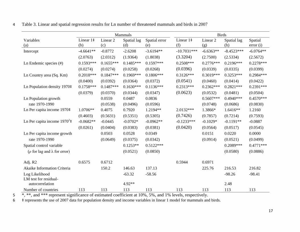
In Table 3, columns b and f, we present linear model results using 2007 data on

population density and per capita income for specification described in Eq. 2. These results

suggest that, as expected, population density and per capita income are highly significant

predictors of threatened mammals and birds based on cross-section analyses. They also verify

that the number of threatened mammals and birds is highly related to the number of endemic

mammals and birds in continental countries. However, our interest in this paper is to examine the

impact of population and per capita income growth rates on imperilment of mammals and birds.

Thus deviating slightly from cross-section analysis by allowing temporal lag effects to be

reflected on, in Table 3 - columns c and g, we present linear model results by including

population and per capita income growth rates during 1970 to 1990 controlling for 1970

population density and per capita income. The use of 1970 as a base year allows us to model the

temporal lagged effect of predictor variables on the imperilment of mammals and birds reported

in 2007. In addition to the significant and sizable impact of endemic species and country area,

these latter results also suggest that population density of 1970 is a significant predictor of

mammals and birds imperilment in 2007.

Per capita income in 1970 is a significant predictor of the number of threatened birds but not the

number of threatened mammals. The relationship between per capita income and threatened

number of birds appears to be characterized as an inverted U - - the so-called Environmental

Kuznets Curve relationship. However, the rate of per capita income growth has no discernible

impact on either the number of threatened mammals or birds, in these models that do not control

for spatial effects (Table 3 – columns c and g).

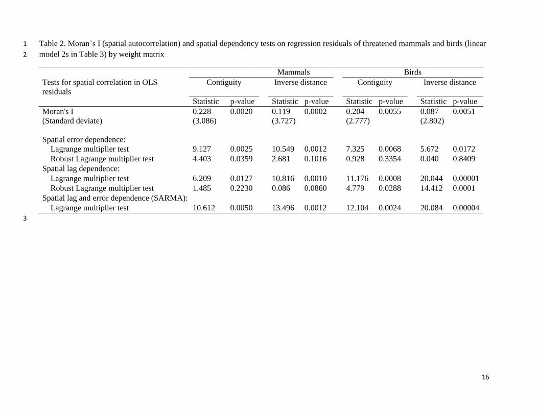
In Table 2, we report the results of the Moran’s I tests for spatial effects (or spatial

autocorrelation) on linear model residuals of models in column c and g for both mammals and

birds. The tests indicate significant spatial autocorrelation on the number of threatened mammals

and birds in a country. The Lagrange multiplier tests on spatial dependency strongly indicate the

presence of spatial lag and error dependency based on two types of weight matrices (simple

contiguity and inverse distance) used to characterise the spatial relationship among observations.

It is worth noting that except the robust version of the Lagrange Multiplier tests based on simple

contiguity matrix for spatial lag and error dependences for mammals and birds, rest of the tests

are consistent for both taxa for both types of weight matrices.


In response to the compelling results from the Moran’s I tests and Lagrange multiplier

tests, we estimated two sets of spatial regressions (spatial lag and spatial error) for both

mammals (Table 3 – columns d and e) and birds (Table 3 – columns h and i) following the model

specified in Eqs. 3 and 4. We used row-standardized simple contiguity based weight matrix and

Maximum Likelihood estimation technique to estimate these models. The model results vary

7

slightly between spatial lag and error specifications for both the taxa as the spatial control

variable differs in its formation between the two types of models.

One important and consistent aspect of our estimation results of spatial models is the

influence of the number of endemic mammals and birds on the number of threatened mammals

and birds. Depending on the spatial models (d, e, h, and i), a 1% increase in the number of

endemic mammals is associated with a 0.15% (or 0.16%) increase in the number of threatened

mammals. Birds are relatively more sensitive to endemism compared to mammals - - a 1%

increase in the number of endemic birds is associated with a 0.22% (or 0.23%) increase in the

number of threatened birds. Land area appears to be highly significant predictor of threatened

mammals and birds across all model specifications, suggesting that an increase in land area could

provide additional habitat for these taxa but also increases the number of threatened mammals

and birds. Likewise, human population density in 1970, a measure of human footprint, has a

statistically significant and consistent impact on threatened mammals and birds in all models.

The per capita income in 1970 has a model-specific influence on the number of threatened

mammals and birds in 2007. Among spatial models (d, e, h, and i), both the linear and quadratic

terms are statistically significant (to indicate EKC type relationship) only in the model where the

spatial effect is controlled by the lag of correlated errors (for mammals) and the lag of the

number of threatened birds (for birds). This is further reinforced by the model selection

diagnostics. For mammals, both Akaike Information Criteria (AIC) and Log likelihood (LL)

values as well as residual autocorrelation tests on spatial lag model (Table 3) indicate superiority

of spatial error model. Whereas for birds, despite similar AIC and LL values for both spatial

models, spatial lag model is marginally preferred as no significant residual autocorrelation is

found in this model. The spatial control variables, row weighted lagged dependent variable (rho)

and lagged error (lambda), are consistently significant across models indicating that control for

spatial effects is important in examining imperilment of mammals and birds. The parameter

estimates of the spatial control variable also suggest that the lagged correlated errors (0.51 vs.

0.48) and lagged number of threatened species (0.21 vs. 0.13) have relatively high influence on

the number of threatened mammals and birds, respectively. For example, a 1% increase in the

weighted average of the threatened birds in the adjoining countries is associated with a 0.21%

increase in the number of threatened birds in the referent country.


Contrary to our expectation, the average rate of per capita income growth during 1970 to 1990

has no significant impacts on the number of threatened mammals and birds in 2007, i.e. the

lagged effect of income growth rate has no direct impact on threatened mammals and birds listed

in IUCN RedList in 2007. Similarly, the average rate of population growth has no discernible

impacts on the number of threatened mammals; but it has uniform and highly significant impact

on the number of threatened birds (models g, h, and i). On average, a 1% increase in the mean

population growth rate between 1970 and 1990 is associated with 0.46%, 0.49% and 0.56%

increase in the percentage of threatened birds based on spatial error, spatial lag and linear (g)

model results, respectively. One potential reason for different results between lag and error

8

models for a given variable is due to the strong correlation of the variable with the lagged error

term i.e. the spatial control variables used in the error models.

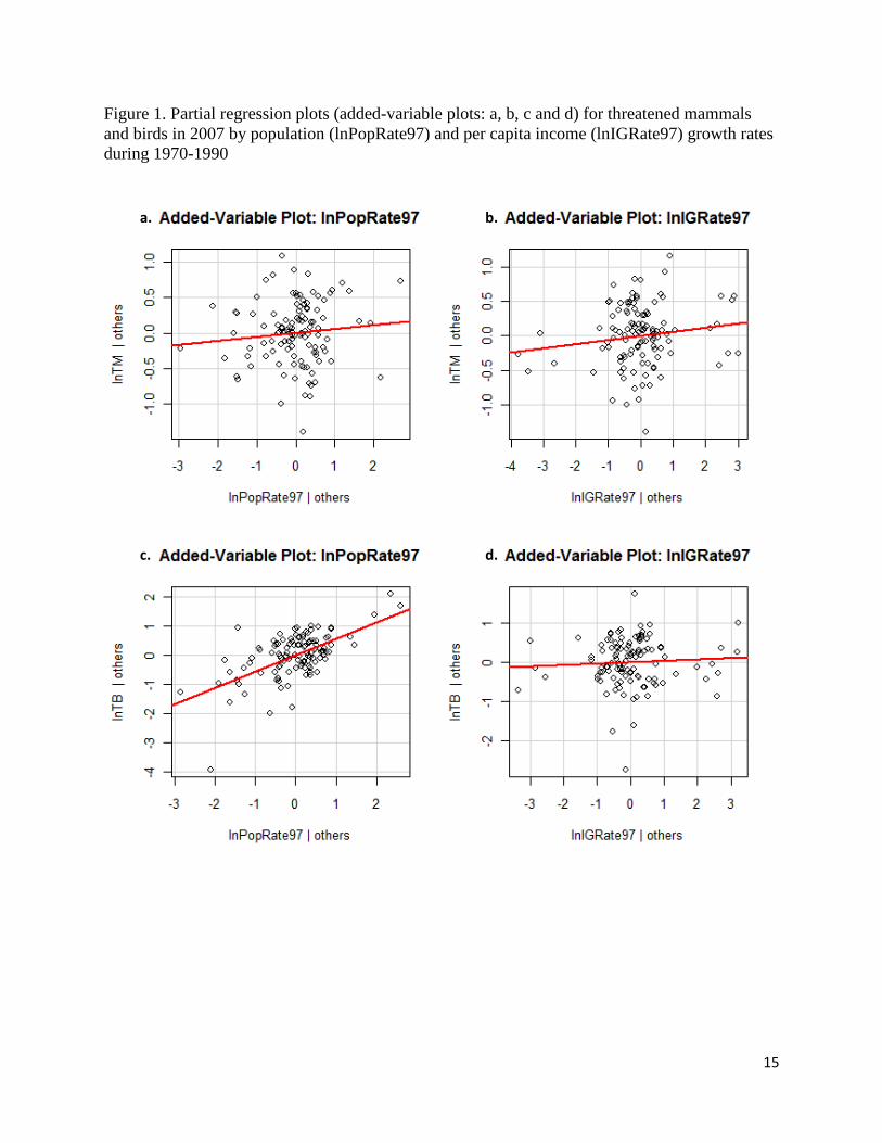
The partial-regression plots in Figure 1 also reinforce our findings of only significant impact of

population growth rate during 1970 to 1990 on the number of threatened birds in 2007. These

plots are drawn using regression residuals from two types of linear models where y-axis

represents the residuals of a model where dependent variable (log-transformed number of

threatened mammals (lnTM) and birds (lnTB) is regressed on explanatory variables excluding

the variable of interest - - lnPopRate97, lnIGRate97); and x-axis represents the regression

residuals when the variable of interest is regressed against all other explanatory variables.

Besides figure 1.c, we didn’t find a strong correlation between these two types of residuals in

Figure 1.

[Figure 1 about here]

4. Discussion

The possibility that imperilment of mammals and birds may be affected by the rate of

population and per capita income growth in addition to population density and per capita income

level is not supported consistently across the taxa and models we examined. Irrespective of

model formulations, we find a consistent positive relationship between population growth rates

and the number of threatened birds, indicating that birds are more sensitive to population growth

rate than mammals. However, we find that the 1970 population density in a country and the rate

of population growth during 1970 to 1990 are more influential factors to predict the number of

threatened birds, but not mammals, in 2007 than the 1970 per capita income level and its growth

rate during the same period of two decades.

In a study that looked at the influence of raising population size on threats to birds and mammals,

McKinney (2001) found that, for continental countries, the log of population explains 16-33% of

the variation in the threat level of birds and mammals. The pattern of the continental population-

threat correlation indicates that per capita human impacts is initially very high and

asymptotically diminish with increasing population size (McKinney 2001). Our findings are

consistent with the sizable impact of human population density on the number of threatened

species reported by McKee et al. (2003).

With respect to the impacts of 1970 income and income growth rate during 1970 to 1990

on threatened mammals and birds, our results depends on model specifications. The impact of

income on threatened mammals and birds show a strong EKC type relationship when we analyse

the cross-section data by considering space for time (models b and f) without controlling for any

temporal and spatial effects. With the control for such effects in the model, the relationship is

sensitive to the model formulations. For example, controlling for correlated errors among

observation we find expected influence of 1970 per capita income on the number of threatened

mammals; and the similar influence of per capita income on the number of threatened birds is

observed while we control for the spatial lag, i.e. the average number of the threatened birds in

9

neighbouring countries. A detailed discussion on EKC type relationship between income and

environmental indicators is beyond the scope of this paper, but a good review on this topic can

be found in Torras and Boyce (1998) and Stern (2004).

For income growth rate we find no significant result for mammals and birds irrespective of

model specifications. In an earlier U.S.-based study, Chambers et al. (2008) found no significant

impacts of per capita income growth between 1972 and 2004 on threatened and endangered

species listings in the States. However, their study differs from ours in two respects: 1) they used

time series data while we used cross-sectional data and 2) they did not check and control for

spatial effects in their model while we do so; and therefore the results are not directly

comparable.

The explanations for why the rate of per capita income growth in earlier period (1970-

1990 in this case) does not seem to matter much in explaining threatened species could be

numerous. One possible reason could be an increase in cleaner service sectors as economies

grow (Kongsamut et al., 2001). Increase in per capita income growth as a result of growth in

service sectors may have little or no negative impacts on the environment. Further, the increased

income might result in greater demand for programs and policies that protect species. This seems

plausible in the case of developed countries where significant emphasis has been given in the last

4 decades to improve the environment by introducing new legislation and programs. We still

observe economic growth at the cost of a deteriorating environment in developing countries (i.e.

tropical deforestation, increased air and water pollutions due to industrial development etc.), but

our model failed to detect the impact of per capita income growth expressed in terms of these

latter trends on threatened species in this analysis.

In addition to the introduction of environmental legislations among countries in the past 4

decades, the insignificant relationship between per capita income growth rate and threatened

mammals and birds could also be due to the impact of environment friendly technological

progresses. Undoubtedly, since the 1970s polluting technologies have been replaced by more

environment friendly technologies in order to advance economic growth in many nations,

particularly in developed countries, that could have potentially reduced the conflict between per

capita income growth rate and the status of threatened species.

Our analyses raise issues regarding how the link between threatened species and its

determinants in a cross-country context is modelled. For example, how temporal effects and

spatial effects are captured in the model; what would be the reasonable temporal lag for a causal

relationship between independent and dependent variables; and what type of spatial effect is

more important for a given research context. To model spatial effects, the choice between the

two spatial models commands further consideration depending on the empirical questions in

hand. If the concern is on spill-over effect of threatened species from neighbouring countries,

obviously lag models would be favored. However, if researchers are exploring the effect of

factors that are not included in the model then error models would be favored. We find better

performance of the error model for mammals and the lag model for birds based on the model

selection criteria used in this analysis – higher Log Likelihood and lower AIC. Thus, depending

upon the empirical questions in hand, both type of models need to be considered in the analysis.

10

However, we are cautious with respect to the findings that there are no lagged effects of

population growth rate on mammals and per capita income growth rates on both threatened

mammals and birds. These findings should be viewed in light of the data availability and

timeframe under investigation. The available data on all model variables for large number of

countries doesn’t go far earlier than 1970; therefore the potential questions and empirical results

about what if we would have examined the effects of these growth rate variables based on a

longer time period is unanswered. But we do acknowledge that this is an important question that

needs further investigation.

There are some limitations in our study that need to be pointed out as well. First of all, we

are limited by the comparable time series data on threatened mammals and birds between any

two periods. Analysis based on the time series data would be more informative than the cross-

sectional data that we used in this analysis, however to the best of our knowledge no consistent

time series data are available on threatened mammals and birds for the period we have

considered. Secondly, we have not been able to capture the potential roles of legislation and

programs that have impacted the country-specific population and per capita income growth rates

and thereby the status of threatened species over the years. Our analysis only provides a general

overview of the relationship between the status of threatened mammals and birds and the

population and per capita income growth rates across continental countries. Since species

imperilment is a complex process and additional empirical studies would benefit to disentangle

this process further and to improve our understanding to take potential actions to slow down or

revert this process.

5. Conclusion

We found mixed results in examining the relationship between the population and per

capita income growth rates in earlier period (1070-1990) and the number of threatened mammals

and birds in a later period (in 2007) among 113 continental countries. Despite significant effect

of population density, the increase in population growth rates during the decades of 1970s and

1980s increases the number of threatened birds in 2007. But no significant effect on both

threatened mammals and birds is found as a result of increase in per capita income growth rates

during the same period. The lack of statistical significance between per capita income growth

rate and the number of threatened mammals and birds is an interesting finding in itself, but it

demands cautions. It needs further research with varying length of the temporal lag covering

longer periods and using updated data on the status of threatened mammals and birds in future

studies.

In the context of our analysis, the population growth rate is more sensitive to species imperilment

than the per capita income growth rates. The implied meaning of our finding is that not only the

human population density but also the human population growth rate is important for

conservation policy. In other words, everything else equal, countries with high population

growth rates at present may face higher number of threatened species, particularly birds, in the

future. Other than increased competition for space/habitat due to increased human population

size as a result of high population growth rate, the causal mechanism of the effect on the number

of threatened species is not quite clear to us; but it is imperative that current conservation

11

policies should also aim to deal with human population density and the population growth rate to

achieve conservation goals in a distant future.

From an analytical perspective, we conclude that a control for spatial effects on cross country

studies is essential to accurately estimate the model parameters. As Tobler’s (1970) first law of

geography states that “everything is related to everything else, but near things are more related

than distant things”, species imperilment has also been influenced by this law. The significance

of this law can be seen based on the model performance (AIC) that both the spatial lag and

spatial error models performed better than the identical model without any control for spatial

effects. Incorporating spill-over effects in cross-country conservation practices such as landscape

level conservation or trans-boundary conservation is important for conservation of threatened

species that have wider home range, i.e. extending into neighbouring countries, or are affected by

human activities in neighbouring countries.

Acknowledgements

This paper was presented at the 55th

Annual AARES National Conference held in

Melbourne, Victoria (February 2011); we appreciate the helpful comments received from

conference participants. We also thank anonymous reviewers for their valuable comments and

suggestions.

References

Anselin, L. (1988). Spatial Econometrics: Methods and Models. Kluwer Academic Publishers,

Dordrecht, The Netherlands.

Anselin, L. (2010). Thirty years of spatial econometrics, Papers in Regional Science 89, 3-25.

Asafu-Adjaye, J., 2003. Biodiversity loss and economic growth: A cross-country analysis.

Contemporary Economic Policy 21, 173-185.

Balmford, A., Bond, W., 2005. Trends in the state of nature and their implications for human

well-being. Ecology Letters 8, 1218-1234.

Bivand, R.S., Pebesma, E.J. and Gómez-Rubio, V. (2008). Applied spatial data analysis with R.

Springer.

Chambers, C.M., Chambers, P.E., Whitehead, J.C., 2008. Economic Growth and Threatened and

Endangered Species Listings: A VAR Analysis, Working Papers. University of Central

Missouri, Department of Economics & Finance, p. 25.

Conservation International (CI), 2010. Global deal to save biodiversity a key step in preventing

extinctions and conserving critical habitats, Available from

http://www.conservation.org/newsroom/pressreleases/ (accessed December 2010).

Dietz, S., Adger, W.N., 2003. Economic growth, biodiversity loss and conservation effort.

Journal of Environmental Management 68, 23-35.

12

Forester, D.J., Machlis, G.E., 1996. Modeling human factors that affect the loss of biodiversity.

Conservation Biology 10, 1253-1263.

Heston, A., Summers, R., Aten, B., 2009. Penn World Table Version 6.3. Center for

International Comparisons of Production, Income and Prices at the University of

Pennsylvania. Available from http://pwt.econ.upenn.edu/php_site/pwt_index.ph (accessed

October 2010).

Hoffmann, M., et al., 2010. The Impact of Conservation on the Status of the World's Vertebrates.

Science 330, 1503-1509.

International Union for Conservation of Nature (IUCN), 2007. The IUCN red list of threatened

species. IUCN, Species Survival Commission, Gland, Switzerland. Available from

http://www.iucnredlist.org/info/tables (accessed January 2008)

Kerr, J.T., Currie, D.J., 1995. Effects of human activity on global extinction risk. Conservation

Biology 9, 1528-1538.

Kongsamut, P., Rebelo, S., Xie, D.Y., 2001. Beyond balanced growth. Review of Economic

Studies 68, 869-882.

McKee, J.K., Sciulli, P.W., Fooce, C.D., Waite, T.A., 2003. Forecasting global biodiversity

threats associated with human population growth. Biological Conservation 115, 161-164.

McKinney, M.L., 2001. Role of human population size in raising bird and mammal threat among

nations. Animal Conservation 4, 45-57.

McPherson, M.A., Nieswiadomy, M.L., 2005. Environmental Kuznets curve: threatened species

and spatial effects. Ecological Economics 55, 395-407.

Mikkelson, G.M., Gonzalez, A., Peterson, G.D., 2007. Economic Inequality Predicts

Biodiversity Loss. Plos One 2, e444.

Moran, P.A.P., 1950. Notes on Continuous Stochastic Phenomena. Biometrika 37, 17-23.

Naidoo, R., Adamowicz, W.L., 2001. Effects of economic prosperity on numbers of threatened

species. Conservation Biology 15, 1021-1029.

NBL, 2010. Rethinking Global Biodiversity Strategies: Exploring structural changes in

production and consumption to reduce biodiversity loss, Netherlands Environmental

Assessment Agency (NBL), The Hague/Bilthoven, p. 170.

Pandit, R., Laband, D.N., 2007a. Threatened species and the spatial concentration of humans.

Biodiversity and Conservation 16, 235-244.

Pandit, R., Laband, D.N., 2007b. Spatial autocorrelation in country-level models of species

imperilment. Ecological Economics 60, 526-532.

Pandit, R., Laband, D.N., 2009. Economic well-being, the distribution of income and species

imperilment. Biodiversity and Conservation 18, 3219-3233.

Pereira, H.M., Leadley, P.W., Proenca, V., Alkemade, R., Scharlemann, J.P.W., Fernandez-

Manjarres, J.F., Araujo, M.B., Balvanera, P., Biggs, R., Cheung, W.W.L., Chini, L.,

Cooper, H.D., Gilman, E.L., Guenette, S., Hurtt, G.C., Huntington, H.P., Mace, G.M.,

Oberdorff, T., Revenga, C., Rodrigues, P., Scholes, R.J., Sumaila, U.R., Walpole, M.,

2010. Scenarios for Global Biodiversity in the 21st Century. Science 330, 1496-1501.

R, 2010. R: A language and environment for statistical computing, R Foundation for Statistical

Computing. R Development Core Team, Vienna, Austria. Available from http://www.R-

project.org/.

Sala, O.E., Chapin, F.S., Armesto, J.J., Berlow, E., Bloomfield, J., Dirzo, R., Huber-Sanwald, E.,

Huenneke, L.F., Jackson, R.B., Kinzig, A., Leemans, R., Lodge, D.M., Mooney, H.A.,

13

Oesterheld, M., Poff, N.L., Sykes, M.T., Walker, B.H., Walker, M., Wall, D.H., 2000.

Biodiversity - Global biodiversity scenarios for the year 2100. Science 287, 1770-1774.

Secretariat of the Convention on Biological Diversity (SCBD), 2010. Global Biodiversity

Outlook 3, SCBD, Montréal, p. 94.

Sodhi, N.S., Bickford, D., Diesmos, A.C., Lee, T.M., Koh, L.P., Brook, B.W., Sekercioglu, C.H.,

Bradshaw, C.J.A., 2008. Measuring the Meltdown: Drivers of Global Amphibian

Extinction and Decline. Plos One 3, e1636.

Stern, D.I. (2004). The Rise and Fall of the Environmental Kuznets Curve, World Development

32, 1419-1439.

The Economics of Ecosystems and Biodiversity (TEEB), 2010. Mainstreaming the Economics of

Nature: A synthesis of the approach, conclusions and recommendations of TEEB.

Available from http://www.teebweb.org/ (accessed October 2010), p. 36.

Tobler, W. (1970). A computer movie simulating urban growth in the Detroit region, Economic

Geography 46, 234-240.

Torras, M. and Boyce, J.K. (1998). Income, inequality, and pollution: a reassessment of the

environmental Kuznets Curve, Ecological Economics 25, 147-160.

World Bank (WB), 2010. World Bank Open Data by Indicators. Available from

http://data.worldbank.org/ (accessed October 2010).

Zibaei, M., Sheykh, Z.A.A., 2009. Biodiversity and economic growth: a cross-country (with

emphasis on developing countries). Journal of Environmental Studies 35, 61-72.

14

Table 1. Descriptive statistics for model variables (n=113 countries©)

Variable Mean

Std.

Deviation Range

Threatened mammals (#) 18.65 16.24 1 to 89

Endangered mammals (#) 10.54 24.49 0 to 155

Total mammals (#) 190.73 117.88 8 to 578

Threatened birds (#) 18.18 21.29 0 to 122

Endangered birds (#) 15.22 31.8 0 to 207

Total birds (#) 649.47 317.29 151 to 1851

Population in 1970 (in 10,000) 2602.83 9386.49 11.13 to 81831.50



Country area (in 10,000 sq km) 85.85 177.76 0.07 to 998.47

Population density 1970 (person/sq.km) 77.29 284.82 0.80 to 2964.29



Population growth from 1970 to 1990

(in 10,000) 1212.04 4145.46 3.44 to 31687

Average rate of population growth per

annum 1970-1990 0.7083 0.7779 0.02205 to 7.31108

Real per-capita income 1970 (int. $) 1512.53 1887.01 149.75 to 13748.79



Per-capita income growth from 1970

to 1990 (int. $) 4514.48 5526.60 102.07 to 26374.27

Average rate of per-capita income growth

per annum 1970-1990 3.1172 2.0773 0.1093 to 13.7812 © Afghanistan, Albania, Algeria, Angola, Argentina, Austria, Bangladesh, Belgium, Belize, Benin, Bhutan, Bolivia,

Botswana, Brazil, Burkina Faso, Burundi, Cambodia, Cameroon, Canada, Central African Republic, Chad, Chile,

China, Colombia, Congo, Democratic Republic of Congo, Costa Rica, Cote d'Ivoire, Denmark, Djibouti, Ecuador,

Egypt, El Salvador, Equatorial Guinea, Ethiopia, Finland, France, Gabon, Gambia, Germany, Ghana, Greece,

Guatemala, Guinea, Guinea-Bissau, Guyana, Honduras, India, Iran, Iraq, Israel, Italy, Jordan, Kenya, Kuwait, Laos,

Lebanon, Lesotho, Libya, Luxembourg, Malawi, Malaysia, Mali, Mauritania, Mexico, Mongolia, Morocco,

Mozambique, Namibia, Nepal, Netherlands, Nicaragua, Niger, Nigeria, Norway, Oman, Pakistan, Panama, Papua

New Guinea, Paraguay, Peru, Poland, Portugal, Qatar, Romania, Rwanda, Saudi Arabia, Senegal, Sierra Leone,

Singapore, Somalia, South Africa, South Korea, Spain, Sudan, Suriname, Swaziland, Sweden, Switzerland, Syria,

Tanzania, Thailand, Togo, Tunisia, Turkey, Uganda, United Arab Emirates, United States, Uruguay, Venezuela,

Viet Nam, Zambia, and Zimbabwe.

15

Figure 1. Partial regression plots (added-variable plots: a, b, c and d) for threatened mammals

and birds in 2007 by population (lnPopRate97) and per capita income (lnIGRate97) growth rates

during 1970-1990

a. b.

d. c.

16

Table 2. Moran’s I (spatial autocorrelation) and spatial dependency tests on regression residuals of threatened mammals and birds (linear 1

model 2s in Table 3) by weight matrix 2

Mammals Birds

Tests for spatial correlation in OLS

residuals

Contiguity Inverse distance Contiguity Inverse distance

Statistic p-value Statistic p-value Statistic p-value Statistic p-value

Moran's I

(Standard deviate)

0.228

(3.086)

0.0020 0.119

(3.727)

0.0002 0.204

(2.777)

0.0055 0.087

(2.802)

0.0051

Spatial error dependence:

Lagrange multiplier test 9.127 0.0025 10.549 0.0012 7.325 0.0068 5.672 0.0172

Robust Lagrange multiplier test 4.403 0.0359 2.681 0.1016 0.928 0.3354 0.040 0.8409

Spatial lag dependence:


Robust Lagrange multiplier test 1.485 0.2230 0.086 0.0860 4.779 0.0288 14.412 0.0001

Spatial lag and error dependence (SARMA):


3

17

Table 3. Linear and spatial regression results for Ln number of threatened mammals and birds in 2007 4

Mammals Birds

Variables

(a)

Linear 1‡

(b)

Linear 2

(c)

Spatial lag

(d)

Spatial error

(e)

Linear 1‡

(f)

Linear 2

(g)

Spatial lag

(h)

Spatial

error (i)

Intercept -4.6641** -0.8772 -2.6208 -3.6194**

-10.7031*** -6.6363** -8.4523*** -6.0764**

(2.0763) (2.0312) (1.9364) (1.8038)

(3.3204) (2.7500) (2.5334) (2.5672)

Ln Endemic species (#) 0.1593*** 0.1655*** 0.1485*** 0.1597***

0.2508*** 0.2776*** 0.2196*** 0.2278***

(0.0274) (0.0274) (0.0258) (0.0268)

(0.0396) (0.0339) (0.0335) (0.0399)

Ln Country area (Sq. Km) 0.2018*** 0.1847*** 0.1969*** 0.1806***

0.3126*** 0.3019*** 0.3253*** 0.2984***

(0.0400) (0.0392) (0.0364) (0.0372)

(0.0541) (0.0460) (0.0414) (0.0422)

Ln Population density 1970‡ 0.1758*** 0.1487*** 0.1630*** 0.1136***

0.2313*** 0.2362*** 0.2821*** 0.2391***

(0.0379) (0.0370) (0.0344) (0.0347)

(0.0623) (0.0532) (0.0481) (0.0504)

Ln Population growth 0.0559 0.0487 0.0836

0.5607*** 0.4940*** 0.4570***

rate 1970-1990

(0.0538) (0.0496) (0.0596)

(0.0748) (0.0686) (0.0830)

Ln Per capita income 1970‡ 1.0706** 0.4075 0.7920 1.2194**

2.0132*** 1.3866* 1.6416** 1.2160

(0.4603) (0.5631) (0.5351) (0.5305)

(0.7426) (0.7857) (0.7214) (0.7593)

Ln Per capita income 19702‡ -0.0682** -0.0445 -0.0702* -0.0962**

-0.1233*** -0.1029* -0.1191** -0.0887

(0.0261) (0.0404) (0.0383) (0.0381)

(0.0420) (0.0564) (0.0517) (0.0545)

Ln Per capita income growth 0.0503 0.0528 0.0349

0.0151 0.0220 0.0000

rate 1970-1990

(0.0649) (0.0375) (0.0342)

(0.0914) (0.0521) (0.0499)

Spatial control variable 0.1253** 0.5122***

0.2089*** 0.4771***

(ρ for lag and λ for error)

(0.0521) (0.0850)

(0.0580) (0.0886)

Adj. R2 0.6575 0.6712

0.5944 0.6971

Akaike Information Criteria

150.2 146.63 137.13

225.76 216.53 216.82

Log Likelihood

-63.32 -58.56

-98.26 -98.41

LM test for residual-

autocorrelation

4.92**

2.48

Number of countries 113 113 113 113

113 113 113 113

*, **, and *** represent significance of estimated coefficient at 10%, 5%, and 1% levels, respectively. 5 ‡ represents the use of 2007 data for population density and income variables in linear 1 model for mammals and birds. 6

Impacts of Population and Income Growth Rates on ... · Impacts of Population and Income Growth...

Documents

Transcript of Impacts of Population and Income Growth Rates on ... · Impacts of Population and Income Growth...