Impacts of Large-scale Wind and Solar PowerIntegration on California’s Net Electrical Load

Hamid Shakera,∗, Hamidreza Zareipoura, David Wooda

aSchulich School of Engineering, University of Calgary, Calgary, Alberta, Canada, T2N1N4

Abstract

Integration of wind- and solar-based generation into the electric grid has signifi-

cantly grown over the past decade and is expected to grow to unprecedented levels

in coming years. Several jurisdictions have set high targets for renewable energy

integration. While electric grid operators have managed the variable and non-

dispatchable nature of wind and solar power at current levels, large-scale inte-

gration of these resources would pose new challenges. In particular, the variable

nature of wind and solar may lead to new electric grid operation and planning

procedures.

Net load in electric grids is defined as the conventional load minus the non-

dispatchable generation. Net load is the basis of operation planning in day-to-

day delivery of electricity to the consumers. With large-scale integration of wind

and solar power, the net load in the system would be significantly affected. In

this paper, we focus on characteristics of net load in electric grids when a large

amount of wind and solar power generation is integrated into the grid. We use

∗Corresponding authorEmail address: hshakera@ucalgary.ca (Hamid Shaker)

Preprint submitted to Elsevier April 19, 2016

the data from California’s power system. California intends to produce 33% of its

electricity from renewable resources by 2020, 80% of which is expected to come

from wind and solar power. We use both historical data and simulated scenarios

of future wind and solar power generation. For future scenarios, we use the data

provided by National Renewable Energy Laboratory to generate wind and solar

power integration scenarios for years 2018 and 2023. The simulated net load data

are analyzed from a variety of perspectives, such as, average daily shapes, load

and net load factor, duration curves, volatility, and hourly ramps. The results

showed that compared to conventional load, characteristics of net load would be

significantly different and need to be taken into account when designing measures

and mechanisms for operating electric grids with high penetration of renewables.

Keywords: Net load; variable generation; large-scale wind and solar integration;

California renewable energy portfolio.

1. Introduction

California’s renewable portfolio standard mandates the state to supply 33%

of its electric energy demand through renewables by 2020 [1]. It is expected

that 80% of the mandate to come from solar and wind power [2]. The three main

investor owned utilities in California, i.e., Pacific Gas and Electric, San Diego Gas

and Electric and Southern California Edison, collectively supplied 22.7% of their

retail electricity through renewables in 2013 [1]. This indicates that the utilities

are working to meet the mandate.

The increasing trend in large-scale integration of renewables, in particular,

2

wind and solar power, is universal. In 2014, the cumulative global installed wind

capacity reached 370 GW, which had nearly a 250 GW increase compared to

2008 [3]. The cumulative global wind capacity is higher than the total installed

generation capacity of Japan, the third largest power system in the world [4].

China and the USA have the highest wind capacity by reaching 114.6 GW and

65.9 GW in 2014, respectively [3]. Among the United States, California power

system with nearly 6 GW wind power capacity ranks second after Texas with

about 16.5 GW [5].

Solar Photovoltaic (PV) power generation capacity also increased substan-

tially over the past few years. Global solar PV capacity has grown from 1.3 GW in

year 2000 to 138.9 GW at the end of 2013 [6]. According to the International En-

ergy Agency (IEA), solar power could potentially provide one third of the global

final energy demand after 2060 [7]. In the USA, on average, the annual solar ca-

pacity has grown more than 40% since 2006 [8]. California is the leader in the

United States. Only in 2013 California installed 2,746 MW of new solar power

capacity, nearly half of the total United States’ new solar PV installations [9]. By

mid 2014, nearly 8 GW of solar PV had received environmental permits to come

online in California [2, 10].

The current integration trends indicate an inevitable major role for wind and

solar in future power systems. However, both wind and solar are known to be non-

dispatchable or variable generation sources for the most part. Operation planning

in conventional power systems has been based on a forecast of future load, an

understanding of the random variations in the load, and the chances of major con-

3

tingencies in the supply system. With the large-scale integration of wind and solar

generators, a new source of uncertainty is added to the operation planning prob-

lem. Wind and solar generators are often treated as non-dispatchable units that

inject power to the grid when available. Thus, in systems with substantial wind

and solar power sources, net load, i.e., the non-dispatchable generation subtracted

from the conventional load becomes the new planning measure. The inherent vari-

ability of the wind and solar power, however, makes the net load time series a more

volatile one compared to the conventional load time series. The higher variability

and less predictability of the net load induces more cycling of the conventional

units, which causes more wear-and-tear and higher maintenance costs [11]. In

[12], the challenges of significant wind and solar integration were categorized

in their low capacity credit, reduced utilization of dispatchable plants, and over-

produced generation. It was mentioned that a system with a higher proportion of

generators which are incapable of rapid entry and exit to the electricity market can

face more challenges when low or negative net load appears. Moreover, high wind

and solar power generation would decrease the average utilization and therefore

the life-cycle generation of the dispatchable units. This increases the generation

costs of supplying the net load [12]. This could potentially result in losing revenue

and in extreme cases bankruptcy of those units.

The concept of net load and the challenges that may arise from its variabil-

ity has been discussed in the literature. In particular, a number of studies on

evaluating and modelling the flexibility requirements of power systems with high

penetration of renewables have considered net load [13, 14, 15, 16, 17, 18, 19].

4

It is argued in [13] that with the current level of wind and solar power, the con-

ventional load variations still makes the highest source of variability and uncer-

tainty in power systems. However, higher wind and solar penetrations along with

adaptation of smart grid technologies, such as demand response, will significantly

increase the variability and uncertainty of the net load. In [14], flexibility re-

quirements of large-scale variable generation were quantified based on simulated

values of onshore wind and solar PV power production in 27 European countries.

It is shown in [14] that increasing wind and solar power generation above a 30%

share in annual electricity consumption will significantly increase flexibility re-

quirements. It is suggested in [15] that in order to decrease the costs associated

with the increased variability of net load in future power systems, new market de-

signs with flexible ramping capability may become a necessity. Flexible ramping

refers to the ability of the system to ramp up/down the generation or load to sta-

bilize system frequency. In [16], using an insufficient ramp resource expectation

algorithm, the flexibility requirements for a system with high variability in the net

load were quantified. Transmission network constraints were considered in [17]

to assess the flexibility of a power system based on the variability of the net load

data. Furthermore, the work in [18] proposed a new power system planning model

by considering large integration of renewable energy sources and the correspond-

ing required flexibility of dispatchable generation units. It has been observed that

with more wind capacity in the system, a part of the base-load generation units

is replaced by mid-load and peak-load generation units due to decrease of the to-

tal net load and increasing its volatility. Finally, in [19], flexibility requirements

5

of high wind and solar PV integrated power system of Germany were analyzed

considering both production flexibility of conventional power plants and storage.

The results showed that high penetration of variable generation does not decrease

the peak net load much. However, the equivalent full load hours decrease signif-

icantly. The occurrence of hours with zero or negative net load also increases.

Moreover, their results suggested that combination of wind and solar PV produc-

tion leads to less storage requirement compared to only wind power generation.

Storage is one of the options to cope with the challenges of renewable power

generation. The benefits of energy storage in providing system flexibility and

controlling negative net load situations have been investigated in a number of

studies [19, 20, 21, 22, 23, 24]. It was found that energy storage can reduce cycling

of conventional power plants and improve the efficiency of power system [21].

Reference [22] provided a comprehensive analysis by combining a simulation of

the impacts of future variable renewables on net load with a focus on surplus-

related storage requirements in Germany. The author concluded that renewable

surpluses can be minimized by decreasing must-run requirements. The storage

requirement would also decrease if power curtailment and demand response were

utilized. Furthermore, storage in distribution systems in Germany was analyzed

in [23]. The results suggested that in the current situation storage may not be

economically viable. However, in high penetration levels storage could be one

of the options to ensure system security. In fact, an adequate mix of technical

initiatives, load shifting and demand side management, and energy storage are

required for high penetration of renewables [24].

6

In other research works, the net load time series has been the basis for build-

ing unit commitment studies [25, 26, 27, 20], studying the market impact of a

price-maker wind unit [28], determining the optimal level of reserves [29], and

managing systems with large numbers of electric vehicles [30].

Despite the increasing importance of understanding how the system net load

and its characteristics would change as the share of renewables grows, the litera-

ture focusing on this topic is limited. In [31], the annual and seasonal changes of

load duration curves after integrating renewable resources, mainly biomass, has

been studied. In this work, less than 5% of renewable generation capacity comes

from wind and solar power. Moreover, there are several studies carried out by the

industry on impacts of large-scale wind and solar power integration on power sys-

tems. Examples include the Eastern wind integration study [32], the Western wind

and solar integration study [33], the California power system study [34, 35, 36],

the Nova Scotia renewable integration study [37] and the New England wind inte-

gration study [38]. While net load has been the basis of such studies, neither has

particularly focused on characteristics of the net load time series.

The objective of the current work is analyzing the impacts of large-scale wind

and solar power integration on the characteristics of net load time series. Based on

a range of wind and solar integration scenarios generated for the case of Califor-

nia’s power system, we study the impacts of renewables on the following aspects:

• Average hourly values,

• Load and net load factor

7

• Load and net load duration curves,

• Load and net load volatilities,

• Hourly ramps.

The main contribution of this paper is to provide an in-depth discussion on how

the net load characteristics would deviate from what power systems are accus-

tomed to today and highlight the challenges that large-scale integration of these

two resources may impose to power systems. Understanding those deviations

would be necessary for power system operators to plan and adjust their operation

strategies, procedures and policies to ensure power system security and reliability

with presence of large-scale wind and solar power.

The rest of the paper is organized as follows. The description of net load defi-

nition and the data is discussed in Section 2. Methodologies for future generation

scenarios are provided in Section 3. Section 4 focuses on the assessment of the

net load from different perspectives. Finally, the paper ends with the conclusions

in Section 5.

2. Background and Data

In this section, first we provide a generic definition for net load. We also

provide a description of the data that has been used in this study.

2.1. Net Load Definition

Assume the value of the conventional load at time interval t is Lt, and the

value of “negawatt” at time interval t to be NGt. The value of net load at time t is

8

defined as

NLt = Lt − NGt. (1)

Typical examples of “negawatt” include the non-disptachable power generated

by wind, solar or small of-the-river hydro facilities [26, 25, 16, 14, 15, 31, 39].

For example, in Alberta’s electricity market, wind power plants do not bid in the

market and inject their available power to the system. The system operator treats

them as negative load in scheduling practices [40]. However, in some studies,

the non-conventional load in the system (e.g., electric vehicle fleet load [30] or

the import/export [13]) has been deducted from the conventional system load to

determine system net load.

2.2. Description of the Data

In order to analyze the effect of large-scale wind and solar on the net load, we

have used the historical hourly load data [41], and wind and solar power genera-

tion data [42] of the California power system from year 2000 to the end of year

2013. These data contain the gradual growth of wind and solar power integra-

tion over this period. According to the California ISO website [43], California’s

power system had 60,703 MW of installed capacity with a recorded peak demand

of 50,270 MW by January 2014. The year 2013 historical data shows a peak solar

PV generation of 2,830 MW and peak wind generation of 4,215 MW. These num-

bers are relatively small compared to the peak load at this year, i.e., 44,924 MW.

However, meeting the 33% renewable goal of year 2020 would require a signifi-

9

cantly larger share of wind and solar generation capacity. To simulate larger levels

of wind and solar power integration in California in the present study, we have

used the data produced by the National Renewable Energy Laboratory (NREL),

which is further discussed next.

In the Western wind and solar integration study [33], NREL, in conjunction

with a few other institutions such as GE Energy Consulting Group, performed a

study to analyze the effect of integrating large amounts of wind and solar power

into the Western US power systems. The first phase of this study investigated

the benefits and challenges of integrating up to 35% wind and solar energy in

the Western Interconnection, by 2017. The second phase evaluated the effect of

wind and solar generation on wear-and-tear costs and emissions associated with

cycling of fossil-fuelled generation fleet [44]. Over the course of these studies,

two datasets have been developed for wind and solar generation [45, 46]. These

datasets are both simulated data, validated against some real-life weather data.

The Western wind dataset is for the years 2004 to 2006 with a 10-minute reso-

lution. The surface covering the Western interconnection power system was mod-

elled with a resolution of 2 km × 2 km grids, and 32,043 locations were selected

across the modelled surface. Each grid point was estimated to hold ten Vestas V90

3 MW wind turbines. For the selected grid points, simulated wind speed data, and

accordingly wind power, were generated [45, 47]. The solar dataset was created

for year 2006 and has the resolution of 5 minutes. It consists of 6,000 simulated

PV plants. Potential solar plants have been detected, and simulated solar power

generation for the plants were created [46].

10

We use the actual data of year 2013 for our analysis. In addition, we use the

NREL datasets to build two sets of scenarios, one for year 2018 and the other for

year 2023, with 5-year intervals from year 2013. The NREL dataset only has solar

data for year 2006, and for consistency, we also use the wind data of the NREL

dataset for year 2006. In addition, actual system load of 2006 is used as the base

for creating the load scenarios for years 2018 and 2023. This is because there

is an inherent correlation between weather conditions, wind/solar generation and

electrical load in a power system. Thus, the load, wind, and solar data of the same

year have been used. Further details on how the wind, solar, and load scenarios

are generated are provided next.

3. Generated Simulated Data Scenarios

In this section, and based on the data described in the previous section, the

generated simulated load, wind power, solar power, and net load scenarios are

discussed.

3.1. The Load Scenarios

We have used the latest publicly available report on load forecast for California

as the basis for our future load scenarios [48]. This report covers the period of year

2012 to 2022. Table 1 summarizes the non-coincident peak load of years 2006,

2018, and 2023 for low, medium, and high load growth rates. The peak load

scenarios for year 2023 in this table are extrapolated based on business as usual

load growth following year 2022 load forecast.

11

Table 1: Historical and forecasts of California non-coincident peak load.Forecast (MW) Increase over 2006 (%)

Year Actual (MW) Low Medium High Low Medium High2006 64,000 – – – – – –2018 – 64,500 67,500 69,000 0.78 5.47 7.812023 – 67,200 71,500 74,900 5.00 11.72 17.03

To limit the number of scenarios in this study, we only use the medium growth

case. Load scenarios for years 2018 and 2023 are generated by scaling up the

hourly load values of year 2006 at the medium growth rates of Table 1, i.e., 5.47%

and 11.72%, respectively. The two future load scenarios are referred to as L18

and L23 for years 2018 and 2023, respectively.

3.2. The Wind Power Production Scenarios

The California power system has three major zones, namely NP15, ZP26 and

SP15. These zones cover the north, central and southern parts of California, re-

spectively. Zone SP15 covers parts of Nevada and Arizona too. These three zones

are marked in Fig. 1.

At the time of writing this paper, there were 2,823 MW of wind capacity in

NP15 and 4,969 MW in SP15. ZP26 currently does not have any wind facilities

[49]. Note that these numbers are the nameplate capacity of the facilities. Some

of them are not fully operational at the time. We assumed that they would be

fully operational by year 2018. In addition, the generation queue of California

Independent System Operator (Cal-ISO) [50] shows 660 MW new wind capacity

planned in the NP15 to be commissioned by the end of 2018. It also shows 3,036

MW new wind capacity for ZP26 and 1,270 MW new capacity in SP15. Although

12

Table 2: The existing capacity and the amount in the generation queue for wind plants in eachzone or county for the California electric power system.

County ZoneExisting windcapacity (MW)

New wind cap.in the queue (MW)

NP15 2,823SP15 4,969

Alameda NP15 Southwest 36Kern ZP26 South 3,036

Riverside SP15 Centre 150San Diego NP15 Southwest 419

Solano NP15 Centre 205Baja California SP15 1,120

Sum (MW) 12,758 7,792 4,966

the generation queue only shows the list of projects under study or approval and it

does not guarantee the projects to be online by the expected online date, it provides

a reasonable indication of what will happen in the future. Hence, we have used

the generation queue as the basis to build our future scenarios, i.e., we assume the

generation queue will be fully realized.

Table 2 summarizes the existing and future wind plants for each zone or

county. It shows that currently California has 7,792 MW wind capacity and it

is expected to add 4,966 MW new wind capacity by the end of year 2018. The

data of Table 2 is used in the following sections to select appropriate places to

represent the year 2018 and also year 2023 wind generation. The objective here is

to select the sites in each zone or sub zone that represent the wind generation of

future scenarios as closely as possible to the future expected situation in line with

the generation queue.

13

3.2.1. Selecting Wind Power Plant Sites for Year 2018

Assuming that all of the existing and new wind facilities will be online by year

2018, there will be 3,483 MW capacity in NP15, 3,036 MW capacity in ZP26,

and 6,239 MW in SP15. It will sum up to 12,758 MW of total wind generation

capacity for year 2018, which we call it Scenario W18. There are no wind sites for

ZP26 in the NREL wind dataset. To address this, the closest sites to the southern

border of zone ZP26 will be considered as the ZP26 sites.

The selected wind capacity is a multiplier of 30 MW. We chose 116 sites in

NP15 and 309 sites in SP15, each with a capacity of 30 MW. These were the sites

with better wind regimes. Figure 1 represents the location of all selected sites

from the NREL dataset for year 2018.

3.2.2. Selecting Wind Power Plant Sites for Year 2023

In order to study higher wind penetration levels, six scenarios have been de-

veloped for year 2023. The expected capacity grows by 4,966 MW over the period

of years 2013 to 2018. For generating the year 2023 scenarios, we consider two

cases for the capacity growth: one at a moderate level of 4,000 MW, and another

one with an extreme growth of 8,000 MW. The second case is to observe an un-

expected extreme growth in wind power installations and quantify the expected

net load impacts. The resulting total wind capacity for the year 2023 is 16,750

MW and 20,750 MW, for the two cases. We consider three scenarios in terms of

where the additional capacity will be located. Those three include: (i) the new

capacity is equally distributed in NP15 and SP15; (ii) 75% of all new capacity is

14

Longitude [degrees]-126 -124 -122 -120 -118 -116 -114 -112

Latit

ude

[deg

rees

]

32

34

36

38

40

42

44NP15SP15

NP15

ZP26

SP15

Figure 1: Selected wind sites for year 2018.

where the additional capacity will be located. Those three include: (i) the new

capacity is equally distributed in NP15 and SP15; (ii) 75% of all new capacity is

located in NP15 and 25% in SP15; and, (iii) 75% of all new capacity is located

in SP15 and 25% is located in NP15. The latter two cases are extreme growth in

one area versus the other, and would allow investigation of the consequences of

such cases on net load. We name these scenarios as W23M-EQ, W23M-NP, and

W23M-SP for the case with 16,750 MW total capacity and W23E-EQ, W23E-NP,

and W23E-SP for the case with 20,750 MW total capacity, respectively.

15

Figure 1: Selected wind sites for year 2018.

located in NP15 and 25% in SP15; and, (iii) 75% of all new capacity is located

in SP15 and 25% is located in NP15. The latter two cases are extreme growth in

one area versus the other, and would allow investigation of the consequences of

such cases on net load. We name these scenarios as W23M-EQ, W23M-NP, and

W23M-SP for the case with 16,750 MW total capacity and W23E-EQ, W23E-NP,

and W23E-SP for the case with 20,750 MW total capacity, respectively.

3.3. The Solar PV Power Production Scenarios

Currently, the installed solar PV capacity in NP15, SP15, and ZP26 is, respec-

tively, 1,257 MW, 3,108 MW and 26 MW [49]. The generation queue of Cal-ISO

shows 12,160 MW new solar PV capacity under study to be added to the system

15

Table 3: The existing capacity and the amount in the generation queue for solar PV plants in eachzone or country for the California electric power system.

Country ZoneExisting solar PVcapacity (MW)

New solar PV cap.in the queue (MW)

NP15 1,257 1,008SP15 3,108ZP26 26 4,572

Arizona SP15 South 455Nevada SP15 East 577

SP15 centre 2,960SP15 South 1,731SP15 West 857

Sum (MW) 16,551 4,391 12,160

by the end of year 2018 [50]. Similar to wind scenarios we have used this data to

build the future scenarios.

Table 3 summarizes the aggregated existing and expected solar PV plants for

each zone. This information will be used to select appropriate locations to rep-

resent year 2018 and also year 2023 solar PV power generation. Assuming that

all of the existing and new solar PV facilities will be online by year 2018, the ex-

pected total solar PV capacity in NP15, SP15, and ZP26 will be 2,265 MW, 8,656

MW and 4,598 MW, respectively. Moreover, the expected capacity additions in

the areas in Nevada and Arizona that are within the Cal-ISO jurisdiction are 577

MW and 455 MW, respectively. Thus, the total solar PV generation capacity for

year 2018 is expected to be 16,551 MW.

3.3.1. Selecting Solar Power Plant Sites for Year 2018

The NREL solar database [46] considers different solar plants with a variety

of sizes from 4 MW to 200 MW capacity depending on the characteristics of the

16

Longitude [degrees]-126 -124 -122 -120 -118 -116 -114 -112

Latit

ude

[deg

rees

]

32

34

36

38

40

42

44NP15ZP26SP15

Figure 2: Selected solar PV sites for year 2018.

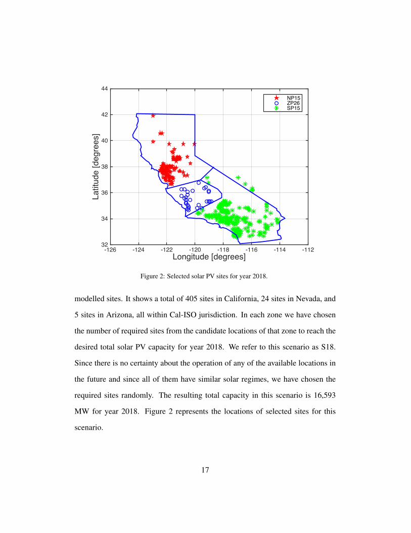
modelled sites. It shows a total of 405 sites in California, 24 sites in Nevada, and

5 sites in Arizona, all within Cal-ISO jurisdiction. In each zone we have chosen

the number of required sites from the candidate locations of that zone to reach the

desired total solar PV capacity for year 2018. We refer to this scenario as S18.

Since there is no certainty about the operation of any of the available locations in

the future and since all of them have similar solar regimes, we have chosen the

required sites randomly. The resulting total capacity in this scenario is 16,593

MW for year 2018. Figure 2 represents the locations of selected sites for this

scenario.

17

3.3.2. Selecting Solar Power Plant Sites for Year 2023

Two scenarios for year 2023 were generated to evaluate the effect of increased

solar PV capacity in this year. Removing the sites that were considered for year

2018, a total of 9,027 MW capacity would remain to be realized. Hence, we have

divided this remaining capacity by two and made two additional scenarios for

year 2023. The first one is built using half the remaining sites and has a total solar

PV capacity of 21,137 MW. This would represent a moderate solar PV capacity

increase, and is referred to as S23M. Considering that more than 12,000 MW solar

PV was expected to come online over the pervious period of years 2013 to 2018,

a 4,513 MW increase in the following five years could be considered moderate.

The sites for this scenario are randomly selected from the remaining choices. The

last scenario includes all of the possible solar PV plants from all of the considered

zones. This leads to a total capacity of 25,620 MW and is referred to as S23E.

This scenario is extremely optimistic, i.e., by the year 2023, all of the potentials

solar power production sites are developed. This, of course, is not unrealistic

considering the extreme solar PV growth over the past years in California and

other places around the world.

3.4. The Net Load Scenarios

Following the aforementioned scenarios for load, wind, and solar PV, there

will be one net load scenario for year 2018 but 12 different net load scenarios for

year 2023. A general description of the net load scenarios is provided in Table 4.

Figure 3 summarizes the net load scenarios for year 2023.

18

Figure 3: The procedure of building net load scenarios using the NREL datasets for year 2023.

The naming style of year 2023 net load scenarios is:

(Solar growth symbol)(Wind growth symbol)-(Wind growth zonal ratio symbol).

In this naming, symbols “M” and “E” represent the Moderate and Extreme growth

rates for solar PV and wind, respectively. “Wind growth zonal ratio symbol” could

be “EQ”, “NP” or “SP” as the equal wind growth rate, 75% new wind growth

rate in NP15, and 75% new wind growth rate in SP15 zones, respectively. For

example, Scenario EM-NP represents the extreme solar PV capacity and moderate

wind capacity, where 75% of new wind installations over year 2018 are considered

in zone NP15.

19

Table 4: Description of year 2023 net load scenarios. MM-EQ∗ means moderate solar growth and extreme wind growthequally distributed between NP15 and SP15 over year 2018.

Growth Rate Over Year 2018 New Wind Capacity Share (%) Scenario NameSolar Wind NP15 SP15 Net Load Solar Wind

Moderate (M) Moderate (M) 50 50 MM-EQ∗ S23M W23M-EQModerate (M) Moderate (M) 75 25 MM-NP S23M W23M-NPModerate (M) Moderate (M) 25 75 MM-SP S23M W23M-SPExtreme (E) Moderate (M) 50 50 EM-EQ S23E W23M-EQExtreme (E) Moderate (M) 75 25 EM-NP S23E W23M-NPExtreme (E) Moderate (M) 25 75 EM-SP S23E W23M-NP

Moderate (M) Extreme (E) 50 50 ME-EQ S23M W23E-EQModerate (M) Extreme (E) 75 25 ME-NP S23M W23E-NPModerate (M) Extreme (E) 25 75 ME-SP S23M W23E-SPExtreme (E) Extreme (E) 50 50 EE-EQ S23E W23E-EQExtreme (E) Extreme (E) 75 25 EE-NP S23E W23E-NPExtreme (E) Extreme (E) 25 75 EE-SP S23E W23E-SP

Table 5 summarizes the all employed scenarios in this study. In this table,

energy penetration level is defined as the annual electricity energy generated by

wind/solar facilities divided by the annual electrical load. The historical solar and

wind capacities in this table are retrieved from [51]. The capacities in the table

only include the large-scale renewable generation.

We believe the developed wind and solar PV capacity growth scenarios over

the period of years 2018 to 2023 are realistic. Based on Table 5, 1,922 MW of

new solar PV capacity was added to the California’s power system over one year

from 2012 to 2013. This means that with the same rate, over a five year period

capacity addition of 9,610 MW is possible. This is even lower than the extreme

solar PV growth of year 2023 in scenarios starting with EM or EE. Moreover, the

extreme wind power growth in our scenarios has 8,000 MW of new installations.

This is equal to the annual average of 1,600 MW, which is not too unrealistic.

Texas alone installed 2,760 MW of new wind capacity during year 2008 [5].

20

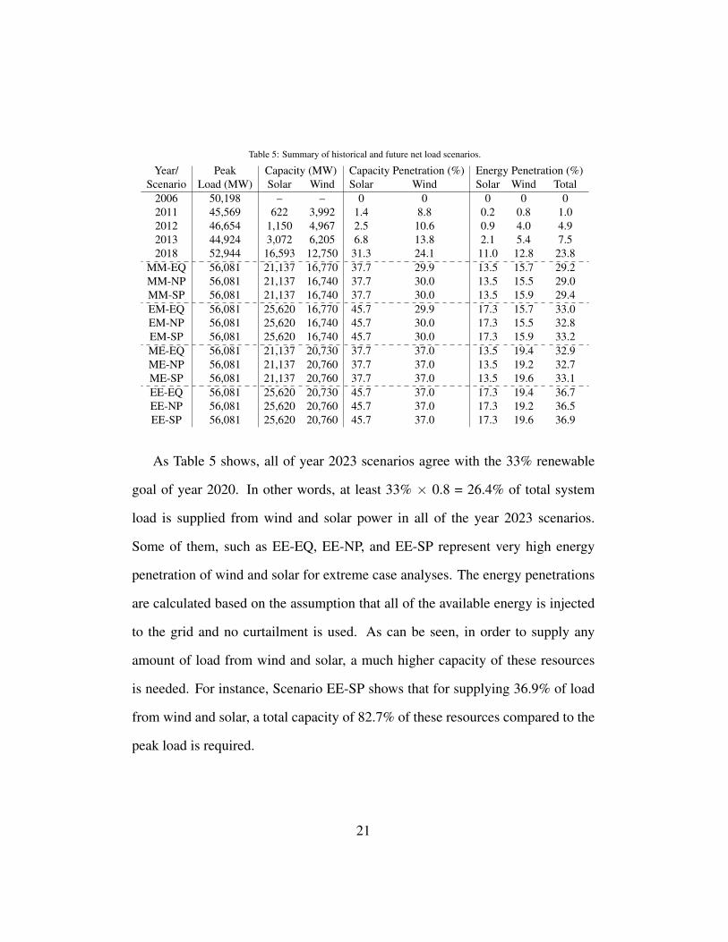
Table 5: Summary of historical and future net load scenarios.

Year/ Peak Capacity (MW) Capacity Penetration (%) Energy Penetration (%)Scenario Load (MW) Solar Wind Solar Wind Solar Wind Total

2006 50,198 – – 0 0 0 0 02011 45,569 622 3,992 1.4 8.8 0.2 0.8 1.02012 46,654 1,150 4,967 2.5 10.6 0.9 4.0 4.92013 44,924 3,072 6,205 6.8 13.8 2.1 5.4 7.52018 52,944 16,593 12,750 31.3 24.1 11.0 12.8 23.8

MM-EQ 56,081 21,137 16,770 37.7 29.9 13.5 15.7 29.2MM-NP 56,081 21,137 16,740 37.7 30.0 13.5 15.5 29.0MM-SP 56,081 21,137 16,740 37.7 30.0 13.5 15.9 29.4EM-EQ 56,081 25,620 16,770 45.7 29.9 17.3 15.7 33.0EM-NP 56,081 25,620 16,740 45.7 30.0 17.3 15.5 32.8EM-SP 56,081 25,620 16,740 45.7 30.0 17.3 15.9 33.2ME-EQ 56,081 21,137 20,730 37.7 37.0 13.5 19.4 32.9ME-NP 56,081 21,137 20,760 37.7 37.0 13.5 19.2 32.7ME-SP 56,081 21,137 20,760 37.7 37.0 13.5 19.6 33.1EE-EQ 56,081 25,620 20,730 45.7 37.0 17.3 19.4 36.7EE-NP 56,081 25,620 20,760 45.7 37.0 17.3 19.2 36.5EE-SP 56,081 25,620 20,760 45.7 37.0 17.3 19.6 36.9

As Table 5 shows, all of year 2023 scenarios agree with the 33% renewable

goal of year 2020. In other words, at least 33% × 0.8 = 26.4% of total system

load is supplied from wind and solar power in all of the year 2023 scenarios.

Some of them, such as EE-EQ, EE-NP, and EE-SP represent very high energy

penetration of wind and solar for extreme case analyses. The energy penetrations

are calculated based on the assumption that all of the available energy is injected

to the grid and no curtailment is used. As can be seen, in order to supply any

amount of load from wind and solar, a much higher capacity of these resources

is needed. For instance, Scenario EE-SP shows that for supplying 36.9% of load

from wind and solar, a total capacity of 82.7% of these resources compared to the

peak load is required.

21

4. Numerical Results and Discussions

In this section, we analyze the developed net load scenarios from a number

of viewpoints. Those include annual and seasonal average shapes, load and net

load factors, load and net load duration curves, renewable energies curtailment

potential, volatility, and hourly ramp analyses. While the specific discussions

are based on the developed scenarios for California, the general directions and

methodologies presented in the paper may be used to evaluate similar issues in

other systems.

4.1. Daily Shoulder and Valley Hours: Load Versus Net Load

In this section, we discuss the shape of net load time series, specifically look-

ing at the valley and shoulder hours, based on annual and seasonal average hourly

values.

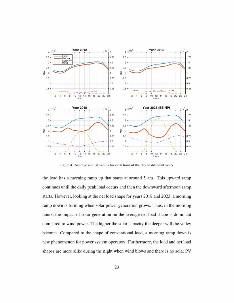
Figure 4 represents the annual average values of net load along with other

variables for each hour of the day for the year 2018 and year 2023 scenarios. We

have also presented the same values for the actual data of years 2012 and 2013 as

references. In this figures, the left vertical axis represents the values of load and

net load, whereas the right vertical axis measures wind and solar PV generation.

We only bring the results for Scenario EE-NP for year 2023. However, other

scenarios also presented similar features.

As this figure shows, comparing the average hourly net load shape for year

2012 with 13.1% wind and solar capacity penetration to year 2023 with 82.7% in

scenario EE-NP, a mid day valley is appearing and growing. For all four years,

22

Hour2 4 6 8 10 12 14 16 18 20 22 24

MW

#104

0.5

1

1.5

2

2.5

3

3.5

4Year 2012 #104

0.25

0.5

0.75

1

1.25

1.5

1.75

2LoadNet loadSolar PVWind

Hour2 4 6 8 10 12 14 16 18 20 22 24

MW

#104

0.5

1

1.5

2

2.5

3

3.5

4Year 2013 #104

0.25

0.5

0.75

1

1.25

1.5

1.75

2

Hour2 4 6 8 10 12 14 16 18 20 22 24

MW

#104

0.5

1

1.5

2

2.5

3

3.5

4Year 2018 #104

0.25

0.5

0.75

1

1.25

1.5

1.75

2

Hour2 4 6 8 10 12 14 16 18 20 22 24

MW

#104

0.5

1

1.5

2

2.5

3

3.5

4Year 2023-(EE-NP) #104

0.25

0.5

0.75

1

1.25

1.5

1.75

2

Figure 4: Average annual values for each hour of the day in different years.

the load has a morning ramp up that starts at around 5 am. This upward ramp

continues until the daily peak load occurs and then the downward afternoon ramp

starts. However, looking at the net load shape for years 2018 and 2023, a morning

ramp down is forming when solar power generation grows. Thus, in the morning

hours, the impact of solar generation on the average net load shape is dominant

compared to wind power. The higher the solar capacity the deeper will the valley

become. Compared to the shape of conventional load, a morning ramp down is

new phenomenon for power system operators. Furthermore, the load and net load

shapes are more alike during the night when wind blows and there is no solar PV

23

power generation. Hence, the overall impact of solar power on the net load shape

is more significant than that of wind power. This is because the average hourly

wind does not vary significantly over a day, whereas the opposite is the case for

solar power generation.

The new net load shape, i.e., a morning downward ramp and an evening up-

ward ramp, would require new power systems operation strategies. Currently, the

system is designed and operated such that enough capabilities for upward ramping

in the morning hours and downward ramping in the evenings are available. Also,

the dispatched units during the morning ramp would be needed for a longer part

of the day as the load grows in the morning and is sustained during the day. How-

ever, with significant solar and wind power integration, the operators must plan

for sufficient capability to ramp down in the morning and ramp up in the evening.

Moreover, since the net load in the high penetration scenarios is generally lower

than the load, conventional generators will be dispatched less often. This may

limit the ramping capability available to the operators since fewer conventional

units may find themselves in the merit order. Thus, the future operation strategies

would need to be adjusted, for both system operators and generation companies,

to ensure system security and economic sustainability.

Another observation from Fig. 4 is that, on average, wind generation peaks

at night time and drops to minimal levels around mid-day. On the other hand,

solar generation peaks during the mid-day when the demand is also high. The

opposite directions of wind and solar generation patterns result in a smoother

net load shape and reduce the morning downward ramp and the evening upward

24

ramp. A smoother net load shape would be more desirable from a planning point

of view because the available transmission and generation infrastructure would

be more evenly utilized. Thus, simultaneous growth of wind and solar power

mitigates some of the challenges associated with these intermittent resources. The

balance between the wind and solar generation capacities are presented in Fig.

5 for Scenario MM-EQ as an example. It depicts the energy penetration level

of wind and solar PV generation together for different load deciles. The decile

penetration of wind and solar individually are not shown in the interests of brevity.

The individual penetrations show the opposite behaviour for the wind and solar

generation. Hence, as Fig. 5 shows, the opposite behaviour of wind and solar

results in an almost flat penetration level for all load levels. This shows the benefit

of simultaneous growth of wind and solar resources in the power system.

Figure 6 presents the seasonal hourly average values for the load and net load

in year 2023. We only bring Scenario MM-EQ as a representation since other sce-

narios behaved similarly. Comparing the four quarters, the upward and downward

net load ramp is significantly higher is Q1 and Q4, i.e., from October to March.

During the period of July to September, i.e., Q3, the net load ramps are the low-

est, and the system would require the least ramping capability. On the other hand,

comparing the load and net load patterns for the four quarters in Fig. 6 one can

observe that the highest ramping capability for conventional load is required dur-

ing Q3. This would call for revisiting the problem of maintenance scheduling in

generation facilities. In particular, maintenance of units that provide the system

with ramping may be shifted to Q3 when the system can spare some units. In

25

Year2013 2018 2023 (MM-EQ)

Pene

tratio

n (%

)

0

5

10

15

20

25

30

35

4040%50%60%70%80%90%100%

Figure 5: Total renewable penetration levels by load decile.

general, the variations in the net load shapes in the four seasons would require

alternative arrangements for providing the system with enough flexibility to deal

with the upward and downward ramps during the day. In [30], the authors discuss

how proper planning of electric vehicle charging could compensate the net load

valley at times. An understanding of the net load shape variations would improve

such plans and help the system in dealing with various issues, such as, high ramps

and low net load at some periods.

4.2. Load Factor and Net Load Factor

Load factor is an indication of how much load changes within a specific period,

typically a year. The ideal load factor for cost and environmental considerations

26

Hour2 4 6 8 10 12 14 16 18 20 22 24

MW

#104

0.5

1

1.5

2

2.5

3

3.5

4

4.5Year 2023-(EE-NP)-Q1 #104

0.25

0.5

0.75

1

1.25

1.5

1.75

2LoadNet loadSolar PVWind

Hour2 4 6 8 10 12 14 16 18 20 22 24

MW

#104

0.5

1

1.5

2

2.5

3

3.5

4

4.5Year 2023-(EE-NP)-Q2 #104

0.25

0.5

0.75

1

1.25

1.5

1.75

2

Hour2 4 6 8 10 12 14 16 18 20 22 24

MW

#104

0.5

1

1.5

2

2.5

3

3.5

4

4.5Year 2023-(EE-NP)-Q3 #104

0.25

0.5

0.75

1

1.25

1.5

1.75

2

Hour2 4 6 8 10 12 14 16 18 20 22 24

MW

#104

0.5

1

1.5

2

2.5

3

3.5

4

4.5Year 2023-(EE-NP)-Q4 #104

0.25

0.5

0.75

1

1.25

1.5

1.75

2

Figure 6: Quarterly average values for each hour of the day for Scenario EE-NP.

is when the load is constant in all times [30].

Although wind and solar power have relatively similar capacity factors over

different years, when their penetration increases, net load factor decreases signif-

icantly compared to the conventional load. For year 2013, the net load capacity

factor was 2% lower than the load factor. However, the load factor of year 2018

is 6.7% lower than that of the conventional load. This decrease is even more for

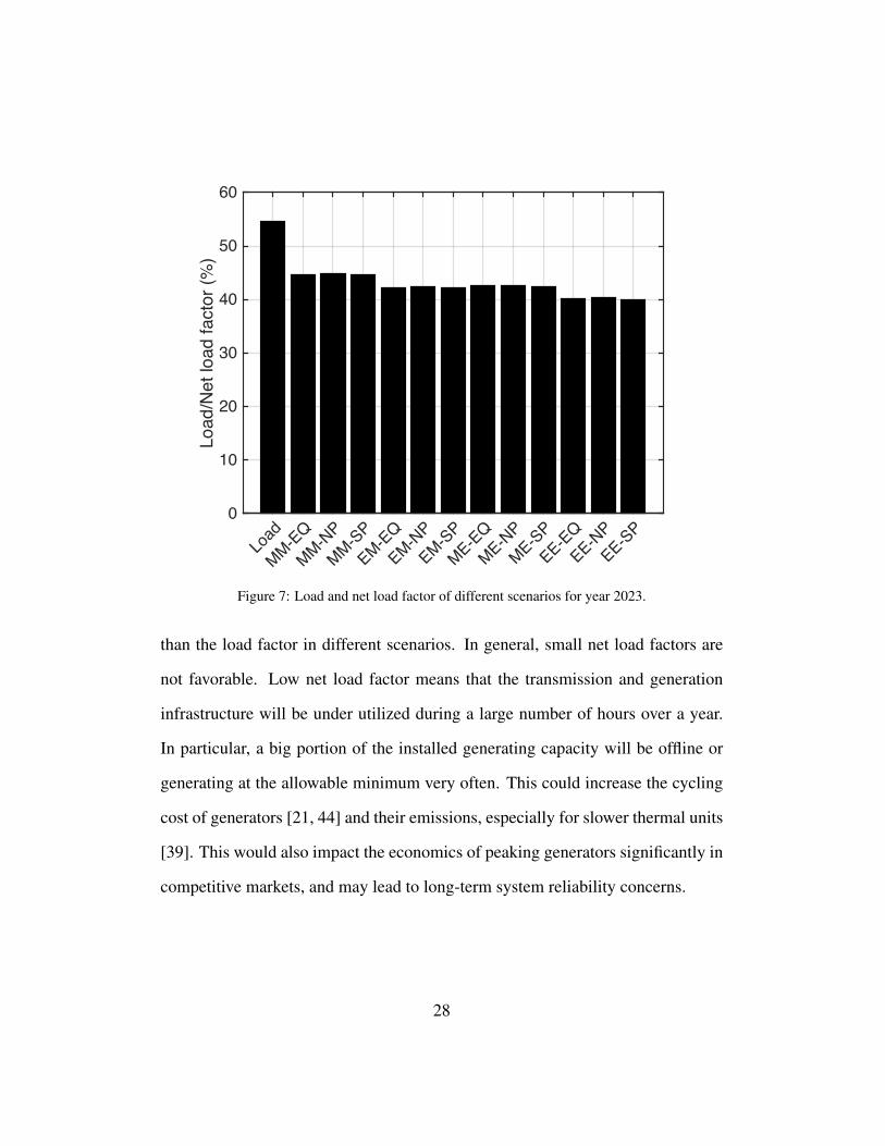
different scenarios of year 2023. Figure 7 represents the net load factors for the

12 scenarios of year 2023 along with the load factor without any wind and solar

power in this year. Observe that the net load factor of year 2023 is 10-15% lower

27

Load

MM-EQ

MM-NP

MM-SP

EM-EQEM-N

PEM-SP

ME-EQME-N

PME-SP

EE-EQEE-N

PEE-SP

Load

/Net

load

fact

or (%

)

0

10

20

30

40

50

60

Figure 7: Load and net load factor of different scenarios for year 2023.

than the load factor in different scenarios. In general, small net load factors are

not favorable. Low net load factor means that the transmission and generation

infrastructure will be under utilized during a large number of hours over a year.

In particular, a big portion of the installed generating capacity will be offline or

generating at the allowable minimum very often. This could increase the cycling

cost of generators [21, 44] and their emissions, especially for slower thermal units

[39]. This would also impact the economics of peaking generators significantly in

competitive markets, and may lead to long-term system reliability concerns.

28

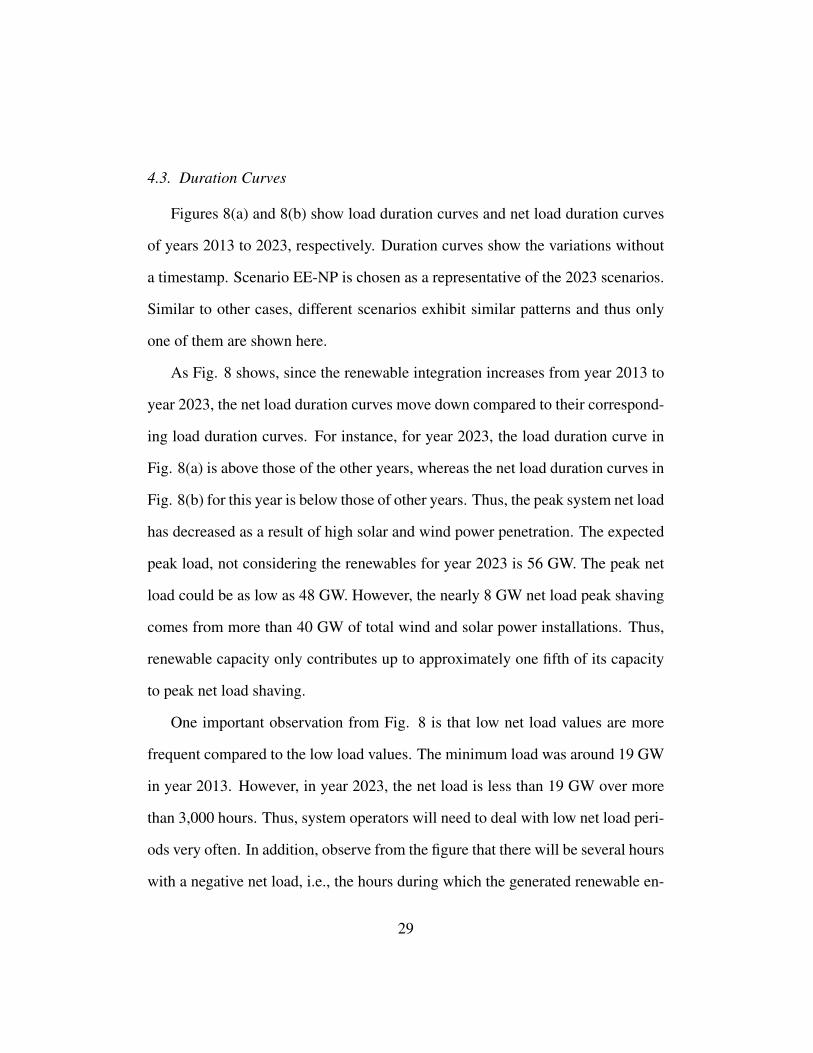
4.3. Duration Curves

Figures 8(a) and 8(b) show load duration curves and net load duration curves

of years 2013 to 2023, respectively. Duration curves show the variations without

a timestamp. Scenario EE-NP is chosen as a representative of the 2023 scenarios.

Similar to other cases, different scenarios exhibit similar patterns and thus only

one of them are shown here.

As Fig. 8 shows, since the renewable integration increases from year 2013 to

year 2023, the net load duration curves move down compared to their correspond-

ing load duration curves. For instance, for year 2023, the load duration curve in

Fig. 8(a) is above those of the other years, whereas the net load duration curves in

Fig. 8(b) for this year is below those of other years. Thus, the peak system net load

has decreased as a result of high solar and wind power penetration. The expected

peak load, not considering the renewables for year 2023 is 56 GW. The peak net

load could be as low as 48 GW. However, the nearly 8 GW net load peak shaving

comes from more than 40 GW of total wind and solar power installations. Thus,

renewable capacity only contributes up to approximately one fifth of its capacity

to peak net load shaving.

One important observation from Fig. 8 is that low net load values are more

frequent compared to the low load values. The minimum load was around 19 GW

in year 2013. However, in year 2023, the net load is less than 19 GW over more

than 3,000 hours. Thus, system operators will need to deal with low net load peri-

ods very often. In addition, observe from the figure that there will be several hours

with a negative net load, i.e., the hours during which the generated renewable en-

29

Hours0 1000 2000 3000 4000 5000 6000 7000 8000 9000

MW

#104

-1

0

1

2

3

4

5

6201320182023-(EE-NP)

Hours0 1000 2000 3000 4000 5000 6000 7000 8000 9000

MW

#104

-1

0

1

2

3

4

5

6

(a)Hours

0 1000 2000 3000 4000 5000 6000 7000 8000 9000

MW

#104

-1

0

1

2

3

4

5

6201320182023-(EE-NP)

Hours0 1000 2000 3000 4000 5000 6000 7000 8000 9000

MW

#104

-1

0

1

2

3

4

5

6201320182023-(EE-NP)

(b)

Figure 8: Duration Curve s: a) Load; b) Net load.

ergy would be more than system demand. Low and negative net load could lead

to potentially challenging security, reliability, and economic sustainability issues.

At very low demand, and to securely plan system operation, many units may be

required to run at their minimum output to ensure system ramping requirements.

Moreover, very low net loads result in difficulties in finding optimum schedules

30

for the dispatchable units [26]. Thus, running at minimum output is inefficient

from the emissions and economics point of view. Negative net load would also re-

quire curtailment of renewable resources or may lead to negative electricity prices

to encourage consumption and discourage generation. Hence, under high penetra-

tion of renewables, the full environmental benefits of wind and solar power may

not be realized. Also, low or negative prices may force some of the peaking units

out of business, which is a system reliability concern in the long-term [29].

For example, on June 16, 2013 between 2 pm and 3 pm, the wholesale electric-

ity price of Germany fell to -100e /MWh. At that time, solar and wind generators

produced 28.9 GW of power, while the total generation was over 51 GW. Since

the grid could not cope with more than 45 GW without becoming unstable, prices

went negative to encourage cutbacks and protect the grid from overgenerating.

The burden of this adjustment fell on gas-fired and coal power plants by decreas-

ing their output to only about 10% of capacity. This means that these units were

losing money on electricity generation [52]. The top 20 energy utilities in Europe

were worth e 1 trillion in year 2008. At the end of year 2013 they were worth less

than half of it. This decrease is due to the changes that wind and solar electricity

generation brought into the grid [52].

In particular, Table 6 summarizes the total energy associated with the negative

net loads for different scenarios for year 2023. The table also shows the num-

ber of hours in each scenario when negative net load occurs. Observe that the

excess energy in the system could be as high as 149 GWh under high renewable

penetration.

31

Comparing the renewable integration scenarios, the amount of excess energy

in the system grows significantly for Scenarios EE-EQ, EE-NP, and EE-SP. The

energy penetration levels for these scenarios are around 36% versus those of the

others that are around 33%. This may indicate that renewable integration to a

certain threshold level may pose significantly less challenges. This means that

after such threshold, adding more renewables may not yield the same incremental

value and needs to be carefully justified.

Also, observe that among scenarios with the same total installed capacity, the

ones with less wind power installations in the south, i.e., SP15, would lead to less

excess energy. For example, the total wind capacity in Scenarios EE-EQ, EE-NP,

and EE-SP is around 21 GW. However, Scenarios EE-NP, where 25% of the wind

additions are in SP15 and the other 75% are in NP15, lead to significantly less

excess energy. This point may be taken into account when providing incentives

for wind power integration programs.

The excess energy in the system may justify the integration of bulk electric

energy storage. Energy storage can reduce cycling and improve the efficiency of

the system as a whole trough significant operating cost savings [21]. At this time,

California has mandated to have 1,325 MW of energy storage capacity by the end

of 2020, which is the United States’ first energy storage mandate [53, 54].

4.4. Volatility

Volatility is a well-known index for measuring changes in a time series. It

measures the standard deviation of changes in a time series over a specific time

32

Table 6: Energies associated with negative net loads in scenarios of year 2023.

ScenarioHours with Negative

Net LoadExcess Energy

(GWh)Total Renewable

Energy Penetration (%)MM-EQ 3 2.1 29.2MM-NP 2 1.0 29.0MM-SP 3 2.2 29.4EM-EQ 20 27.0 33.0EM-NP 16 22.3 32.8EM-SP 21 33.5 33.2ME-EQ 11 18.1 32.9ME-NP 8 16.4 32.7ME-SP 19 29.4 33.1EE-EQ 45 111.9 36.7EE-NP 45 97.2 36.5EE-SP 55 149.0 36.9

window. To calculate the volatility usually the logarithmic return of the time series

over the time period h, denoted by rt,h is used, which is calculated by

rt,h = ln(Lt

Lt−h

) = ln(Lt) − ln(Lt−h). (2)

Lt is the parameter being assessed at time t. Then, standard deviation of logarith-

mic returns over a time window T , denoted by σh,T , is defined as the historical

volatility and calculated by

σh,T =

√∑Tt=1(rt,h − rT,h)2

T − 1, (3)

where rT,h is average of the logarithmic returns over T . Since electricity load

follows daily and weekly periodicities, the return time series are highly correlated

33

and therefore, the time window T should be chosen short enough (e.g. 24 h) so as

to have negligible return correlations [55]. Thus, the historical volatility for each

studied day, denoted by σh,24(d), is calculated as

σh,24(d) =

√∑24×dt=1+24×(d−1)(rt,h − rt,h(d))2

23× 100 (%), (4)

where d stands for the studied day or period of time, and rt,h(d) is the logarithmic

return’s average over the specified day d. Considering hourly, daily, and weekly

logarithmic returns, the averages of σh,24(d) over all studied days, i.e., σ1,24, σ24,24

and σ168,24 are volatility indices. For instance, σ1,24 quantifies the electricity load

or any other time series changes from one hour to another during a day. Because

in some cases we have very low or negative net loads and zero solar generation,

volatility calculation results in very large amounts for those instances. Hence,

we have assumed the floor of 1,000 MW for the time series for the purpose of

volatility analysis.

Table 7 summarizes the volatilities of load and net load over the studied years

and scenarios. Although volatility of load, wind and solar PV do not change

significantly over the years and different scenarios, it is clear from the figure that

with increased level of wind or solar penetration, volatility of the net load notably

increases compared to that of the load. For instance, σ1,24 for the net load in

year 2013 is 5%, which is very close to the load volatility, i.e., 4%. However, in

year 2023, σ1,24 of the net load is 2-3 times higher than the conventional load. In

addition, daily and weekly volatilities of the net load could be up to eight times

34

higher than that of the load in some scenarios. Higher volatility is an indication of

lower predictability for a time series [56]. Thus, with the increasing penetration of

renewables, predicting the net load for operation planning purposes would become

more challenging. Low accuracy in net load forecasts could lead to inefficient

operation schedules, and thus, lower economic and environmental benefits.

The other observation from Table 7 is that the highest net load volatilities are

associated with higher wind capacity in the SP15 zone, i.e., scenarios ending with

-SP. The reason is that aggregated wind time series are smoother with higher geo-

graphically dispersed wind sites in the systemwide values [57]. The scenarios with

the highest net load volatilities are the ones with high wind power installations in

the South. As discussed before, the geographical location of new installations and

the associated impacts on overall success of the renewable integration program

need to be carefully analyzed to gain the highest benefits.

4.4.1. Hourly Volatilities

Volatility indices are also calculated based on each hour of the day for different

scenarios. This will reveal the most volatile hours of the day and the results could

be used later to develop appropriate forecasting engines based on the volatility

of each hour. Since all of the scenarios show similar patterns for each hour, Fig.

9 only shows the load and net load volatilities of Scenario EE-EQ as a sample

along with the results of years 2013 and 2018. To calculate these volatilities, first

the original time series is filtered by each hour and 24 separate time series are

generated. With the new filtered time series, hourly volatilities are based on the

35

Table 7: Annual volatilities for load (L) and net load (NL). All numbers are in %.σ1,24 σ24,24 σ168,24

Scenario / Year L NL L NL L NL2013 4.3 4.7 3.0 4.4 2.9 4.42018 4.8 7.4 3.1 10.3 2.7 10.1

MM-EQ 4.8 9.2 3.1 13.8 2.7 13.6MM-NP 4.8 9.2 3.1 13.2 2.7 13.0MM-SP 4.8 9.3 3.1 14.6 2.7 14.6EM-EQ 4.8 10.2 3.1 17.9 2.7 17.7EM-NP 4.8 10.1 3.1 17.0 2.7 16.8EM-SP 4.8 10.5 3.1 19.5 2.7 19.5ME-EQ 4.8 12.3 3.1 17.3 2.7 17.3ME-NP 4.8 12.3 3.1 16.6 2.7 16.6ME-SP 4.8 12.4 3.1 18.2 2.7 18.4EE-EQ 4.8 13.7 3.1 21.9 2.7 21.9EE-NP 4.8 13.6 3.1 20.9 2.7 20.9EE-SP 4.8 14.0 3.1 23.7 2.7 24.0

changes of one specific hour from one day to another. Hence, all of the volatilities

are actually averaged over a weekly time frame, i.e., T=7.

As Fig. 9(a) depicts, load volatilities are nearly similar for all hours from

year 2013 to 2023. However, net load volatilities in Fig. 9(b) show a significant

increase with the increased level of renewable integration. Note that Fig. 9(b)

shows one of the most volatile cases for year 2023. However, the least volatile

case, which is Scenario MM-NP, shows the peak volatility of 33.6%, which is still

much higher than the 2018 case, i.e., 23.8%. The highest net load volatility is

for Scenario EE-SP with the maximum of 64.5%. This confirms the observations

from Table 7.

Another point from Fig. 9 is that load volatility is higher in the early morning

36

Year2013 2018 2023

Vola

tility

(%)

0

2

4

6

8

10

12 Hour 1Hour 2Hour 3Hour 4Hour 5Hour 6Hour 7Hour 8Hour 9Hour 10Hour 11Hour 12Hour 13Hour 14Hour 15Hour 16Hour 17Hour 18Hour 19Hour 20Hour 21Hour 22Hour 23Hour 24

(a)

Year2013 2018 2023-(EE-EQ)

Vola

tility

(%)

0

10

20

30

40

50

60 Hour 1Hour 2Hour 3Hour 4Hour 5Hour 6Hour 7Hour 8Hour 9Hour 10Hour 11Hour 12Hour 13Hour 14Hour 15Hour 16Hour 17Hour 18Hour 19Hour 20Hour 21Hour 22Hour 23Hour 24

(b)

Figure 9: Hourly volatilities for year 2013 to 2023, Scenario EE-EQ: a) Load; b) Net load.

hours for all of the scenarios, especially from hour 7 to 9. After that the volatilities

decrease and the minimum volatile hours are midnight times. However, the most

volatile net load hours are in the afternoon, typically hours 13 and 14. These are

moments with a high level of solar generation. This means that solar generation

shifts the most volatile hours from morning to early afternoon. One consequence

37

of this situation is that net load forecasts will be less accurate at the time of very

high solar generation, which coincides with the net load valley. This could impose

operation costs since inaccuracy in the net load forecast will result in non-optimal

reserve scheduling for these hours. A detailed analysis on the effect of high after-

noon volatilities and forecasting error on the system operation and reserve costs

would be essential to determine the operational challenges associated with these

moments.

4.5. Hourly Ramp Analysis

In this section, hourly ramps, which are changes from one hour to the next

hour for load and net load scenarios are evaluated. The analyses are performed

for each scenario. However, net load results are almost similar to each other in

scenarios with the same capacity of wind and solar, no matter where the sites are

placed. Hence, similar to previous studies, only one scenario, i.e., ME-NP will be

reported as representative of all cases.

Duration curves of hourly ramps are shown in Fig. 10 for load. As can be

seen, upward hourly ramps with the magnitude of up to 1,000 MW/h are slightly

more frequent compared to downward ramps, specially for years 2018 and 2023.

On the other hand, hourly downward ramps of higher than 1,000 MW/h are more

frequent. Thus, one can conclude that for the load, the duration curve has a longer

tail on the left side, meaning that large downward load ramps are more frequent

than the upward ramps.

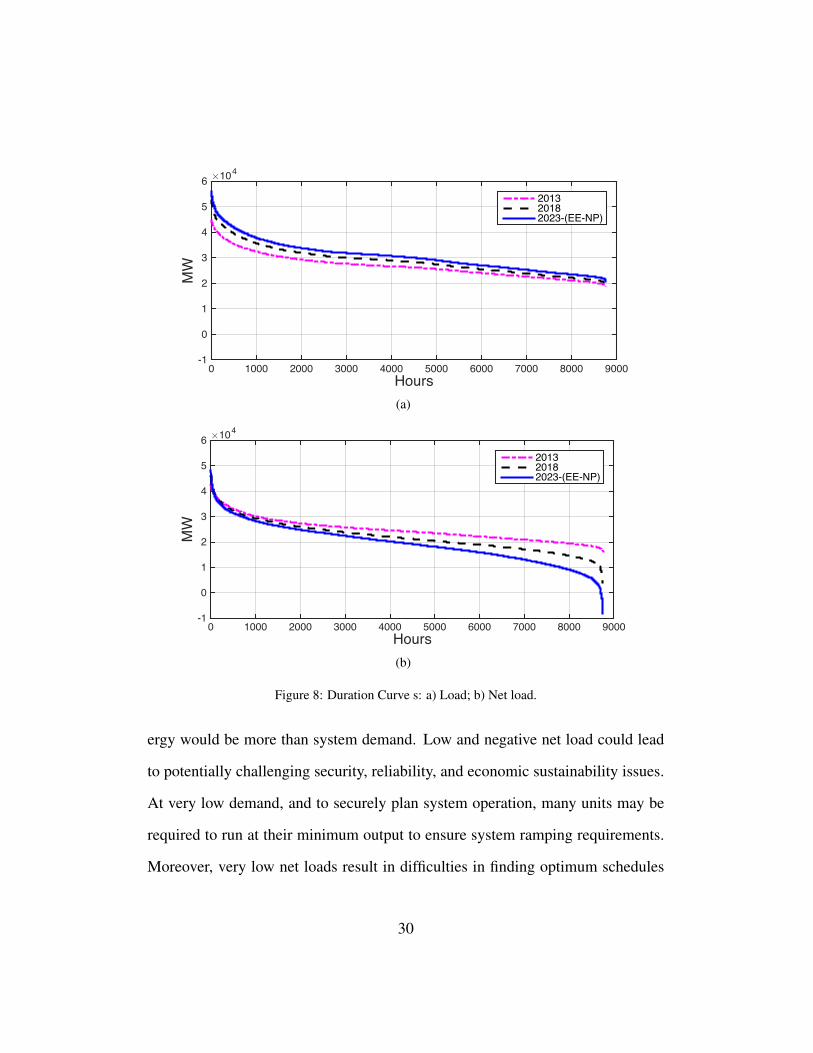
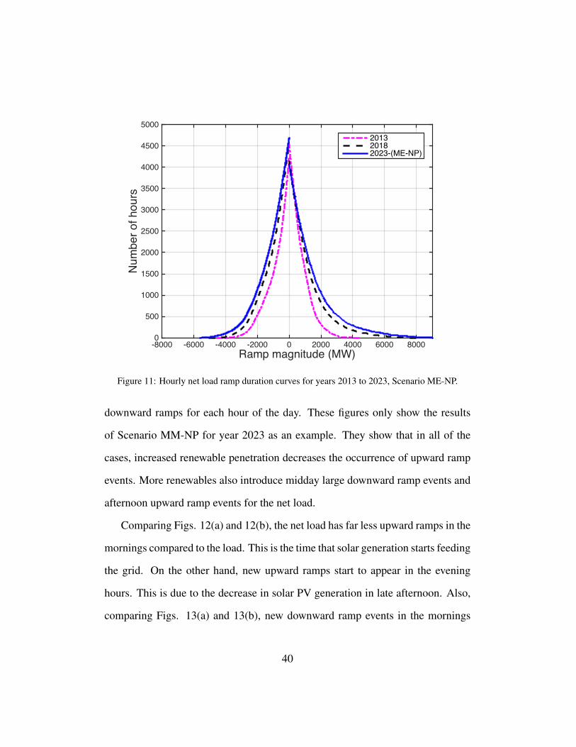
Net load hourly ramp duration curves are depicted in Fig. 11. As this figure

38

Ramp magnitude (MW)-5000 -4000 -3000 -2000 -1000 0 1000 2000 3000 4000

Num

ber o

f hou

rs

0

500

1000

1500

2000

2500

3000

3500

4000

4500201320182023

Figure 10: Hourly load ramp duration curves for years 2013 to 2023 in all scenarios.

shows, net load ramps have the opposite direction compared to that of the load,

i.e., the net load has more frequent very large upward hourly ramps. The other

observation is that as the penetration level of renewables increase, both upward

and downward hourly ramps are far more often compared to that of the load.

Figure 10 shows that the load hourly ramps could be as high as 4,000 MW/h.

However, high penetration level of renewables can lead to upward hourly ramps

of up to 8,000 MW/h, see Fig. 11. This magnitude of hourly ramps would require

careful security measures to avoid any catastrophic system issues.

In order to analyze the ramps in more details, all of the hourly ramps greater

than 1,500 MW/h are counted and depicted in Fig. 12 for upward and Fig. 13 for

39

Ramp magnitude (MW)-8000 -6000 -4000 -2000 0 2000 4000 6000 8000

Num

ber o

f hou

rs

0

500

1000

1500

2000

2500

3000

3500

4000

4500

5000201320182023-(ME-NP)

Figure 11: Hourly net load ramp duration curves for years 2013 to 2023, Scenario ME-NP.

downward ramps for each hour of the day. These figures only show the results

of Scenario MM-NP for year 2023 as an example. They show that in all of the

cases, increased renewable penetration decreases the occurrence of upward ramp

events. More renewables also introduce midday large downward ramp events and

afternoon upward ramp events for the net load.

Comparing Figs. 12(a) and 12(b), the net load has far less upward ramps in the

mornings compared to the load. This is the time that solar generation starts feeding

the grid. On the other hand, new upward ramps start to appear in the evening

hours. This is due to the decrease in solar PV generation in late afternoon. Also,

comparing Figs. 13(a) and 13(b), new downward ramp events in the mornings

40

Year2013 2018 2023

Occ

urre

nce

0

50

100

150

200

250

300

350

400 Hour 1Hour 2Hour 3Hour 4Hour 5Hour 6Hour 7Hour 8Hour 9Hour 10Hour 11Hour 12Hour 13Hour 14Hour 15Hour 16Hour 17Hour 18Hour 19Hour 20Hour 21Hour 22Hour 23Hour 24

(a)

Year2013 2018 2023-(MM-NP)

Occ

urre

nce

0

50

100

150

200

250

300

350 Hour 1Hour 2Hour 3Hour 4Hour 5Hour 6Hour 7Hour 8Hour 9Hour 10Hour 11Hour 12Hour 13Hour 14Hour 15Hour 16Hour 17Hour 18Hour 19Hour 20Hour 21Hour 22Hour 23Hour 24

(b)

Figure 12: Occurrence of upward ramps higher than 1,500 MW/h by hour for year 2013 to 2023,Scenario MM-NP: a) Load; b)Net load.

start to appear as the penetration of renewables grows. This is associated with the

growth of solar power generation in the morning. On the other hand, the midnight

downward ramp events decrease slightly for net load compared to the load, due

to wind power generation. Thus, it can be observed that renewables clearly shift

the upward ramp events from morning to afternoon. Also, solar power is a more

41

Year2013 2018 2023

Occ

urre

nce

0

50

100

150

200

250

300

350

400 Hour 1Hour 2Hour 3Hour 4Hour 5Hour 6Hour 7Hour 8Hour 9Hour 10Hour 11Hour 12Hour 13Hour 14Hour 15Hour 16Hour 17Hour 18Hour 19Hour 20Hour 21Hour 22Hour 23Hour 24

(a)

Year2013 2018 2023-(MM-NP)

Occ

urre

nce

0

50

100

150

200

250

300

350

400 Hour 1Hour 2Hour 3Hour 4Hour 5Hour 6Hour 7Hour 8Hour 9Hour 10Hour 11Hour 12Hour 13Hour 14Hour 15Hour 16Hour 17Hour 18Hour 19Hour 20Hour 21Hour 22Hour 23Hour 24

(b)

Figure 13: Occurrence of downward ramps higher than 1,500 MW/h by hour for year 2013 to2023, Scenario MM-NP: a) Load; b)Net load.

dominant factor in shifting the ramp events timing over a day compared to wind

power. A shift in the timing of ramping events needs to be taken into account

when operation planning procedures are revisited in systems with high renewables

penetration.

42

5. Conclusions

In this paper, we have evaluated the impacts of large-scale wind and solar PV

power integration in the California’s power system on the characteristics of the net

load in the system. The analyses were performed using both historical data, i.e.,

years 2013 and before, and also future simulated data scenarios for years 2018 and

2023. The future scenarios are based on simulated data provided by NREL. The

simulated net load time series are analyzed from a variety of perspectives, such

as, average daily shapes, load and net load factor, duration curves, renewables

curtailment, volatility, and hourly ramps. The main contribution of this paper is to

provide an in-depth discussion on how the net load characteristics would deviate

from what power systems are accustomed to today when a significant amount of

wind and solar power generation is integrated into the grid.

The average daily shapes are analyzed in Section 4.1. The results showed that

high solar PV penetration level would create a valley in the net load during the day

time. This changes the ramping behaviour of net load compared to conventional

load and shifts the morning hourly upward ramps to the afternoon. This change

would require new power systems operation and reserve scheduling strategies.

The analyses in Section 4.2 showed that net load factor decreases compared

to the conventional load when the wind and solar PV penetrations grow. Con-

sequently, the transmission and generation infrastructure will be under utilized

during a large number of hours over a year, which would also impact the eco-

nomics of peaking generators significantly in competitive markets, and may lead

to long-term system reliability concerns.

43

Another observation was made on load and net load duration curves in Section

4.3. Negative and very low net loads in scenarios with significant wind and solar

PV power integration is expected in future years. The negative net loads were

shown to occur more frequently if the majority of new wind capacity installations

take place in the southern areas of the California power system. Negative net loads

would lead to curtailment of renewables or negative prices for electricity in com-

petitive markets. Under high penetration of renewables, the full environmental

benefits of wind and solar power may not be realized. It also leads to inefficient

system operation from the emissions and economics point of views.

The volatility analysis of Section 4.4 showed that high integration of wind

and solar power also results in up to eight times higher volatility of the net load

in future scenarios compared to the conventional load, specially in the case of

high wind capacity growth in southern California. This is an indication of lower

predictability for the net load time series. Forecast of net load time series are the

basis of many operation-planning decisions, and thus, inaccurate net load fore-

casts would be costly to the system.

Finally, an analysis of hourly ramp events in Section 4.5 revealed an increased

level of upward net load ramp events compared to that of conventional load in

future scenarios that have a high penetration level of wind and solar PV genera-

tion. The ramping behaviour of the net load calls for new strategies for market

and system operation to ensure the security of the grid.

44

Acknowledgements

Partial support for this work came from the Canadian National Science and

Engineering Research Council (NSERC) and the ENMAX Corporation under the

Industrial Research Chairs program.

References

[1] California Renewables Portfolio Standard (RPS), http://www.cpuc.

ca.gov/PUC/energy/Renewables/, 2002.

[2] Final Report for Assessment of Visibility and Control Options for Dis-

tributed Energy Resources, California ISO, http://www.caiso.

com/Documents/FinalReport-Assessment-Visibility-

ControlOptions-DistributedEnergyResources.pdf, Ac-

cessed: 2014-01-14, 2012.

[3] Global statistics, Global Wind Energy Council (GWEC), http://

www.gwec.net/global-figures/graphs/, Accessed: 2015-12-

17, 2014.

[4] Electricity-installed generating capacity by country, http:

//mecometer.com/topic/electricity-installed-

generating-capacity/, Accessed: 2014-01-14, 2014.

[5] Installed Wind Capacity, US Department of Energy, http:

45

//apps2.eere.energy.gov/wind/windexchange/wind_

installed_capacity.asp, Accessed: 2015-12-17, 2015.

[6] G. Masson, S. Orlandi, M. Rekinger, Global market outlook for Photo

Voltaics 2014-2018, European photovoltaic industry association (EPIA) .

[7] Solar Energy Perspectives, International Energy Agency (IEA),

http://www.iea.org/publications/freepublications/

publication/Solar_Energy_Perspectives2011.pdf, 2011.

[8] L. Sherwood, U.S. Solar Market Trends 2012, Interstate Renewable En-

ergy Council (IREC), http://www.seia.org/sites/default/

files/IREC_2012%20Solar%20Review.pdf, 2013.

[9] Solar Market Insight Report 2013 Year in Review, Solar Energy In-

dustries Association (SEIA), http://www.seia.org/research-

resources/solar-market-insight-report-2013-year-

review, Accessed: 2014-11-17, 2013.

[10] Tracking Progress: Renewable Energy Overview, http://www.

energy.ca.gov/renewables/tracking_progress/

documents/renewable.pdf, Accessed: 2014-01-14, 2013.

[11] D. Lew, G. Brinkman, N. Kumar, S. Lefton, G. Jordan, S. Venkataraman,

Finding Flexibility: Cycling the Conventional Fleet, IEEE Power Energy

Mag. 11 (6) (2013) 20 – 32, ISSN 1540-7977.

46

[12] F. Ueckerdt, R. Brecha, G. Luderer, Analyzing major challenges of wind and

solar variability in power systems, Renewable Energy 81 (2015) 1 – 10.

[13] N. Navid, G. Rosenwald, Market Solutions for Managing Ramp Flexibil-

ity With High Penetration of Renewable Resource, IEEE Trans. Sustainable

Energy 3 (4) (2012) 784–790, ISSN 1949-3029.

[14] M. Huber, D. Dimkova, T. Hamacher, Integration of wind and solar power

in Europe: Assessment of flexibility requirements, Energy 69 (2014) 236 –

246, ISSN 0360-5442.

[15] B. Wang, B. Hobbs, Flexiramp market design for real-time operations: Can

it approach the stochastic optimization ideal?, in: IEEE Power and Energy

Society General Meeting, ISSN 1944-9925, 2013.

[16] E. Lannoye, D. Flynn, M. O’Malley, Assessment of power system flexibil-

ity: A high-level approach, in: IEEE Power and Energy Society General

Meeting, ISSN 1944-9925, 2012.

[17] E. Lannoye, D. Flynn, M. O’Malley, Transmission, Variable Generation, and

Power System Flexibility, IEEE Trans. Power Systems PP (99) (2014) 1–10,

ISSN 0885-8950.

[18] A. Belderbos, E. Delarue, Accounting for flexibility in power system plan-

ning with renewables , International Journal of Electrical Power & Energy

Systems 71 (2015) 33 – 41.

47

[19] L. Saarinen, N. Dahlback, U. Lundin, Power system flexibility need induced

by wind and solar power intermittency on time scales of 1-14 days, Renew-

able Energy 83 (2015) 339 – 344.

[20] K. Hedegaard, P. Meibom, Wind power impacts and electricity storage - A

time scale perspective, Renewable Energy 37 (1) (2012) 318 – 324.

[21] C. O’Dwyer, D. Flynn, Using Energy Storage to Manage High Net Load

Variability at Sub-Hourly Time-Scales, IEEE Trans. Power Syst. PP (99)

(2014) 1–10, ISSN 0885-8950.

[22] W.-P. Schill, Residual load, renewable surplus generation and storage re-

quirements in Germany, Energy Policy 73 (2014) 65 – 79.

[23] M. Doering, Assessment of Storage Options for Reduction of Yield Losses

in a Region with 100% Renewable Electricity, Energy Procedia 73 (2015)

218 – 230.

[24] B. Azzopardi, A. Gabriel-Buenaventura, Feasibility assessment for high pen-

etration of distributed photovoltaics based on net demand planning , Energy

76 (2014) 233 – 240.

[25] G. Osrioa, J. Lujano-Rojasa, J. Matiasa, J. Catalo, A new scenario

generation-based method to solve the unit commitment problem with high

penetration of renewable energies, International Journal of Electrical Power

& Energy Systems 64 (2015) 1063 – 1072, ISSN 0142-0615.

48

[26] E. Delarue, D. Cattrysse, W. D’haeseleer, Enhanced priority list unit com-

mitment method for power systems with a high share of renewables, Electric

Power Systems Research 105 (2013) 115 – 123, ISSN 0378-7796.

[27] Y. Dvorkin, H. Pandzic, M. Ortega-Vazquez, D. Kirschen, A hybrid stochas-

tic/interval approach to transmission-constrained unit commitment, IEEE

Trans. Power Syst. PP (99) (2014) 1–11, ISSN 0885-8950.

[28] A. de la Nieta, J. Contreras, J. Munoz, M. O’Malley, Modeling the Impact

of a Wind Power Producer as a Price-Maker, IEEE Trans. Power Syst. 29 (6)

(2014) 2723–2732, ISSN 0885-8950.

[29] J. Morales, A. Conejo, J. Perez-Ruiz, Economic Valuation of Reserves in

Power Systems With High Penetration of Wind Power, IEEE Trans. Power

Syst. 24 (2) (2009) 900–910, ISSN 0885-8950.

[30] L. Zhang, F. Jabbari, T. Brown, S. Samuelsen, Coordinating plug-in electric

vehicle charging with electric grid: Valley filling and target load following,

Journal of Power Sources 267 (2014) 584 – 597, ISSN 0378-7753.

[31] K. Chaiamarit, S. Nuchprayoon, Impact assessment of renewable genera-

tion on electricity demand characteristics, Renewable and Sustainable En-

ergy Reviews 39 (2014) 995 – 1004, ISSN 1364-0321.

[32] Eastern wind integration and transmission study, EnerNex Corporation,

http://www.nrel.gov/docs/fy11osti/47078.pdf, Accessed:

2014-01-14, 2010.

49

[33] Western Wind and Solar Integration Study, GE Energy Consult-

ing, prepared for NREL, http://www.nrel.gov/electricity/

transmission/western_wind.html, 2010.

[34] X. Bai, et. al., Intermittency analysis project: Appendix B, impact of inter-

mittent generation on operation of California power grid, GE Energy Con-

sulting, http://www.uwig.org/CEC-500-2007-081-apb.pdf,

Accessed: 2014-07-23, 2007.

[35] Y. Makarov, C. Loutan, J. Ma, P. de Mello, Operational Impacts of Wind

Generation on California Power Systems, IEEE Trans. Power Syst. 24 (2)

(2009) 1039–1050, ISSN 0885-8950.

[36] M. Rothleder, U. Helman, C. Loutan, T. Guo, J. Xie, S. Venkataraman, Inte-

gration of wind and solar under a 20% RPS: Stochastic simulation methods

and results from California ISO studies, in: IEEE Power and Energy Society

General Meeting, ISSN 1944-9925, 2012.

[37] Nova Scotia Renewable Energy Integration Study, GE Energy Consulting,

https://www.nspower.ca/site/media/Parent/2013COSS_

CA_DR-14_SUPPLEMENTAL_REISFinalReport_REDACTED.pdf,

Accessed: 2014-07-23, 2013.

[38] New England Wind Integration Study, GE Energy Consulting, EnerNex Cor-

poration, and AWS Trupower, http://www.uwig.org/newis_es.

pdf, 2010.

50

[39] A. S. Brouwer, M. van den Broek, A. Seebregts, A. Faaij, Impacts of large-

scale Intermittent Renewable Energy Sources on electricity systems, and

how these can be modeled, Renewable and Sustainable Energy Reviews 33

(2014) 443 – 466, ISSN 1364-0321.

[40] 2013 Annual Market Statistics, AESO, http://www.aeso.ca/

downloads/2013_Annual_Market_Statistics.pdf, Accessed:

2014-07-23, 2013.

[41] California ISO OASIS database, http://oasis.caiso.com/

mrioasis/logon.do, Accessed: 2014-01-14, 2014.

[42] California ISO renewables watch, http://www.caiso.com/market/

Pages/ReportsBulletins/DailyRenewablesWatch.aspx,

Accessed: 2014-01-14, 2014.

[43] California ISO: What are we doing to green the grid?, http://www.

caiso.com/informed/Pages/CleanGrid/default.aspx, Ac-

cessed: 2014-01-14, 2014.

[44] G. B. D. Lew, The Western Wind and Solar Integration Study Phase

2, NREL, http://www.nrel.gov/docs/fy13osti/55588.pdf,

Accessed: 2014-07-23, 2013.

[45] NREL Western Wind Dataset, http://www.nrel.gov/

electricity/transmission/western_wind_methodology.

html, Accessed: 2014-01-14, 2014.

51

[46] NREL Solar Power Data for Integration Studies, http://www.nrel.

gov/electricity/transmission/solar_integration_

methodology.html, Accessed: 2014-01-14, 2014.

[47] D. Lew, Development of Regional Wind Resource and Wind Plant Output

Datasets, 3TIER / NREL Technical Monitor, http://www.nrel.gov/

docs/fy10osti/47676.pdf, Accessed: 2014-07-23, 2010.

[48] Bryan Alcorn, et. al., California Energy Demand 2012 - 2022 Final Fore-

cast, California Energy Commission, http://www.energy.ca.gov/

2012publications/CEC-200-2012-001/CEC-200-2012-

001-SF-V1.pdf, Accessed: 2014-07-23, 2012.

[49] Master CAISO Control Area Generating Capability List, https://www.

caiso.com/Documents/GeneratingCapabilityList.xls,

Accessed: 2014-07-23, 2014.

[50] The California ISO Controlled Grid Generation

Queue, https://www.caiso.com/Documents/

ISOGeneratorInterconnectionQueueExcel.xls, Accessed:

2014-07-23, 2014.

[51] Electric Generation Capacity and Energy, Government of California,

http://energyalmanac.ca.gov/electricity/electric_

generation_capacity.html, Accessed: 2014-01-14, 2014.

52

[52] How to lose half a trillion euros, http://www.economist.

com/news/briefing/21587782-europes-electricity-

providers-face-existential-threat-how-lose-half-

trillion-euros, Accessed: 2014-01-14, 2013.

[53] D. Hull, California adopts first-in-nation energy storage plan, San Jose

Mercury news, http://www.mercurynews.com/business/ci_

24331470/california-adopts-first-nation-energy-

storage-plan, 2013.

[54] J. St. John, California Passes Huge Grid Energy Storage Mandate,

Greentechgrid, http://www.greentechmedia.com/articles/

read/california-passes-huge-grid-energy-storage-

mandate, 2013.

[55] I. Simonsen, Volatility of power markets, Physica A : Statistical Mechanics

and its Applications 355 (1) (2005) 10 – 20, ISSN 0378-4371.

[56] H. Zareipour, C. Canizares, K. Bhattacharya, J. Thomson, Application of

Public-Domain Market Information to Forecast Ontario’s Wholesale Elec-

tricity Prices, IEEE Trans. Power Syst. 21 (4) (2006) 1707–1717.

[57] M. Hand, S. Baldwin, E. DeMeo, et. al., Renewable Electricity Futures

Study, Bulk Electric Power Systems: Operations and Transmission Plan-

ning, National Renewable Energy Laboratory (NREL), 2012.

53