Impact of Voucher Design on Public School - NYU Steinhardt
63
IESP Working Paper Series Impact of Voucher Design on Public School Performance: Evidence from Florida and Milwaukee Voucher Program Rajashri Chakrabarti Federal Reserve Bank of New York WORKING PAPER #09-03 March 2009
Transcript of Impact of Voucher Design on Public School - NYU Steinhardt

IESP Working Paper Series
Impact of Voucher Design on Public School Performance:
Evidence from Florida and Milwaukee Voucher Program
Rajashri ChakrabartiFederal Reserve Bank of New York
WORKING PAPER #09-03March 2009

Acknowledgements
.
Editorial Board The editorial board of the IESP working paper series is comprised of senior research staff and affiliated faculty members from NYU's Steinhardt School of Culture, Education, and Human Development and Robert F. Wagner School of Public Service. The following individuals currently serve on our Editorial Board:
Amy Ellen Schwartz Director, IESP
NYU Steinhardt and NYU Wagner
Sean Corcoran NYU Steinhardt
Cynthia Miller-Idriss
NYU Steinhardt
Leslie Santee Siskin NYU Steinhardt
Leanna Stiefel
Associate Director for Education Finance, IESP NYU Wagner
Mitchell L. Stevens
NYU Steinhardt
Sharon L. Weinberg NYU Steinhardt
Beth Weitzman
NYU Wagner
I am grateful to Steve Coate, Ron Ehrenberg and Miguel Urquiola for helpful com-ments, suggestions and encouragement. I thank Robin Boadway, Julie Berry Cullen, Chris Cornwell, Sue Dynarski, Dennis Epple, David Figlio, Caroline Hoxby, Brian Jacob, George Jakubson, Dean Lillard, David Mustard, Tim Sass, Mike Waldman and seminar participants at Cornell University, the University of Georgia, Econometric Society Meetings, Southern Economic Association Meet-ings, American Education Finance Association Conference and Society of Labor Economists Conference for helpful discussions, and the Program on Education Policy and Governance at Harvard University for its postdoctoral support. The views expressed in this paper are those of the author and do not necessarily reflect the position of the Federal Reserve Bank of New York or the Federal Reserve System. All errors are my own.
Abstract
This paper examines the impact of vouchers in general and voucher design in particu-lar on public school performance. It argues that all voucher programs are not created equal. There are often fundamental differences in voucher designs that affect public school incentives differently and induce different responses from them. It analyzes two voucher programs in the U.S. The 1990 Milwaukee experiment can be looked upon as a “voucher shock” program that suddenly made low-income students eligible for vouchers. The 1999 Florida program can be looked upon as a “threat of voucher” program, where schools getting an “F” grade for the first time are exposed to the threat of vouchers, but do not face vouchers unless and until they get a second “F” within the next three years. In the context of a formal theoretical model, the study argues that the threatened public schools will unambiguously improve under the Florida-type program and this improvement will exceed that under the Milwaukee type program. Using school-level scores from Florida and Wisconsin, and a difference-in-differencesestimation strategy in trends, it then shows that these predictions are validated empiri-cally. These findings are reasonably robust in that they survive several sensitivity checks including correcting for mean reversion and a regression discontinuity analy-sis.

1 Introduction
The 1983 report “A Nation at Risk”1 and a series of similar reports have led to continued concern that
American public schools may be lagging behind their counterparts in other parts of the developed world.
This has led to a wave of demands for public school reform. School choice and accountability in general,
and vouchers in particular, are among the most hotly debated instruments of public school reform. This
paper is motivated by the need to understand the effect of vouchers and, in particular, the designs
of different kinds of vouchers on public school performance. It argues that all voucher programs are
not created equal. There are often fundamental differences in voucher designs that affect public school
incentives differently and in turn bring about different responses from them.
The first publicly funded voucher program in the U.S. was initiated in Milwaukee in 1990. This was
followed by Cleveland in 1996 and Florida in 1999. Interestingly, there are crucial differences in the
designs of these programs. The Milwaukee and Cleveland experiments are similar. (In the rest of the
paper, I will concentrate on the Milwaukee experiment because of better data availability.) These two
experiments can be looked upon as “voucher shock” programs with a sudden government announcement
that the low-income public school population is eligible for vouchers. In particular, starting in the 1990-
91 school year, the Milwaukee Parental Choice Program (MPCP) makes all public school students with
family income at or below 175% of the poverty line eligible for vouchers to attend non-sectarian private
schools.
On the other hand, the Florida program can be looked upon as a “threat of voucher” program, rather
than a “voucher shock” program. Here the failing public schools are first threatened with vouchers and
vouchers are implemented only if they fail to meet a government designated cutoff quality level. In
particular, under the Florida opportunity scholarship program, all students of a public school become
eligible for vouchers or “opportunity scholarships” if the school gets two “F” grades in a period of four
years. Therefore, a school getting an “F” for the first time is exposed to the threat of vouchers but does
not face vouchers unless and until it gets a second “F” within the next three years.2,3 This paper argues
1 National Commission of Excellence in Education (1983),“A Nation at Risk: The Imperative for Educational Reform,”Washington, DC: U.S. Government Printing Office.
2 The Florida Department of Education classifies schools according to five grades: -A, B, C, D, F (A-highest, F-lowest).The criteria for the assignment of the lower grades are discussed in section 4.2. For a detailed description of the twoprograms, see Figlio and Lucas (2004) for Florida, and Witte (2000) for Milwaukee.
3 In 1999, 78 schools got an “F”. Students in 2 of those schools became eligible for vouchers. In 2000, 4 elementaryschools got an F although none became eligible for vouchers. In 2001, no school got an F. In 2002, 64 schools got an F.Students in 10 of those schools became eligible for vouchers. In 2003 (2004), students in 9 (21) schools became eligible forvouchers.
1IESP Working Paper #09-03

that these differences in voucher designs will affect public school incentives differently and will induce
very different responses from them. In particular, it argues that the Florida type “threat of voucher”
program will have a much greater effect on public school response and performance than the Milwaukee
type “voucher shock” program.
Apart from the above differences, the designs of the two programs are strikingly similar. In both the
experiments, the private schools are not permitted, by law, to discriminate between students who apply
with vouchers–they have to accept all students unless oversubscribed and have to pick students randomly
once they are oversubscribed. The system of funding is also very similar. Under each program the average
voucher amount equals the state aid per pupil, and the vouchers are financed by an equivalent reduction
of state aid to the district. Thus state funding is directly tied to student enrollment and enrollment losses
due to vouchers are reflected in a revenue loss for the public school.4 The average voucher amounts under
the Florida (1999-2000 through 2001-2002) and Milwaukee (1990-1991 through 1996-1997) programs have
been respectively $3,330 and $3,346. During the corresponding periods, vouchers as a percentage of total
revenue per pupil have been 41.55% in Florida and 45.23% in Milwaukee.
The paper develops its argument in the context of a formal theoretical model with three agents:–the
public school, the households and the private schools. The demand for public school is endogenously
determined from household behavior, giving micro-foundations to the public school payoff function. In
an equilibrium framework, the model endogenously determines public school quality and its ingredients—
public school effort and peer group quality. Both under complete information and under moral hazard
(when public school effort is not observable), the model generates two empirically testable predictions
that hold at the respective program equilibria—the threatened public schools will show an unambiguous
improvement in quality under the Florida-type “threat of voucher” program and the improvement under
the “threat of voucher” program will exceed that under the Milwaukee-type “voucher shock” program.
Using school-level test score data from Florida and Wisconsin, the paper next proceeds to test the
two theoretical predictions. Implementing a difference-in-differences estimation strategy in trends, it
estimates the program effects for each of the experiments by comparing the post-program improvement
of the treated schools with an appropriate set of control schools. Controlling for potentially confounding
4 I will mainly focus on the Milwaukee experiment up to 1996-97. This is because following a 1998 Wisconsin SupremeCourt ruling, there was a major shift in the program when religious private schools were allowed to participate in theprogram and the program entered into its second phase. Moreover, the financing of the Milwaukee program saw somecrucial changes, so that the voucher amounts and the revenue loss per student due to vouchers were not comparablebetween Florida and second phase Milwaukee. Sections 4.5 and 6 discuss the implications of these changes and whether acomparison of the Florida program with Milwaukee second phase is legitimate.
2IESP Working Paper #09-03

pre-program time trends and post-program common shocks, the paper finds considerable evidence in
favor of both the theoretical predictions. These findings are quite robust in that they continue to hold
after controlling for other confounding factors such as mean reversion, possibility of a stigma effect
and withstand several sensitivity tests. I use multiple strategies, including a regression discontinuity
estimation strategy, to address the potential problem of mean reversion. The findings have strong policy
implications from the point of view of public school reform.
A growing body of literature analyzes multiple issues relating to school vouchers. Nechyba (1996,
1999, 2000) analyzes distributional effects of alternative voucher policies in a general equilibrium frame-
work that endogenizes residential choice. Hoyt and Lee (1998) and Chen and West (2000) investigate
the political support for vouchers. Epple and Romano (1998) argue that vouchers lead to sorting by
income and ability. They model private school and household behavior, but assume public schools to
be passive. Epple and Romano (2002) examine how alternative voucher designs can affect stratification
and technical efficiency. They allow for public school technical inefficiencies, but these inefficiencies are
taken to be exogenous in their study. In particular, none of the above studies endogenize public school
quality.
Nechyba (2003) allows for efficiency gain in the public schools facing competition from vouchers.5
However, he does not model public school behavior. Manski (1992) considers the impact of vouchers on
public school expenditure and social mobility, while allowing for rent-seeking public schools. But unlike
the present paper, understanding the impact of different voucher designs on public school performance
is not a concern in Manski. Modeling public school quality, McMillan (2002) shows that under certain
circumstances, public schools may find it optimal to reduce productivity when a voucher is introduced.
The main difference once again is that he considers the effect of traditional voucher experiments (“voucher
shock” in my terminology) on public school response, while this study compares and contrasts the
effects of two types of voucher experiments on public school performance. Second, unlike McMillan,
this paper derives the demand for public school from equilibrium household behavior, thus providing
micro-foundations to the public school payoff function. Third, unlike McMillan, this paper models peer
quality, which is considered to be an essential input in the education production function.
A number of empirical studies look at the effect of vouchers on the performance of students who move
to private schools with vouchers (the “choice students”). For a comprehensive review of this literature,
see Hoxby (2003b) and Rouse (1998). The empirical literature on the impact of vouchers on public
5 He includes two constants in the public school production function that exogenously increase with a decrease in peerquality variance and an increase in the share of private school attendance respectively.
3IESP Working Paper #09-03
school performance has been relatively sparse. Greene (2001, 2003) finds positive effect of the Florida
program on the performance of the treated schools. However, the classification into different treatment
groups in Greene (2003) is based on post-program grades of schools and hence is susceptible to the
endogeneity problem. In response to Greene’s (2001) paper, a spurt of studies took place (Camilli and
Bulkley (2001), Harris (2001), Kupermintz (2001)) that express doubt that the program effect in the
Greene study is contaminated by mean reversion6 and/or stigma effect of getting the lowest performing
grade “F”. However, all of the above studies are potentially afflicted by mean reversion.7 This study
gets rid of these problems by (i) arriving at the mean reversion effect using pre-program data and (ii)
using a regression discontinuity analysis in Florida to estimate the program effect. Another problem
with all the above studies is that they do not control for any pre-program trends, which once again can
bias the program effects.
Analyzing the Florida program and using student level data from a subset of Florida districts, Figlio
and Rouse (2004) find some evidence of improvement of the treated schools in the high stakes state tests,
but these effects diminish in the low stakes, nationally norm-referenced test. Using student level data,
West and Peterson (2005) study the effects of the revised Florida program (after the 2002 grading rule
changes) as well as the NCLB Act on test performance of students in Florida public schools. They find
that the former program has had positive and significant impacts on student performance, but they find
no such effect for the latter. This study differs from the above two studies in some fundamental ways.
First, the question posed here is different. The objective of this paper is to analyze whether voucher
design matters as far as public school performance is concerned. For this purpose, it compares and
contrasts the effects of two alternative voucher designs (Florida and Milwaukee designs) on public school
performance. On the other hand, both Figlio and Rouse (2004) and West and Peterson (2005) focus on
Florida. Second, this study combines a theoretical and an empirical counterpart, while both the above
studies are essentially empirical. Third, the time periods under consideration are also different. West
6 For a discussion of the mean reversion problem in Florida-style programs that base rewards and/or sanctions on schoolscores, see Chay et al. (2003).
7 In Florida, Greene (2001) argues that mean reversion is not a problem in his study as the gains achieved by low scoringF schools are similar to those of the high scoring F schools between 1999 and 2000. However, similar gains of low scoringand high scoring F schools do not imply an absence of mean reversion since 2000 is a post-program year. In fact, even inthe presence of mean reversion, the coefficients of the high scoring and low scoring F schools can be similar if there aredifferential program effects between these two groups. The studies in response to Greene (2001) seek to arrive at meanreversion corrected program effect by subtracting the post-program (2000) score from the predicted score in 2000, where thepredicted score is obtained from a regression of the 2000 score on the pre-program (1999) score. However, in this strategy,the mean reversion effect is confounded with the program effect (since 2000 is a post-program year) and the mean reversioncorrection gets rid of at least part of the program effect. (Harris (2001) and Kupermintz (2001) exclude the F schools intheir predicted score regressions. However, it is not clear that any mean reversion effect from the other groups of schoolscan be attributed to the F schools.)
4IESP Working Paper #09-03

and Peterson study the impact of the revised Florida program (after the 2002 grading rule changes) and
focus on the time period 2002-04. Figlio and Rouse study the effect of the 1999 Florida program, but
they look at the effect of the program in 2000 only, that is, one year after program. This study also looks
at the effect of the 1999 program in Florida, but the time period considered here is different. Given the
nature of the Florida program, the 1999 threatened schools (that is, the schools that received an “F”
grade in 1999) would be exposed to the threat of vouchers for the next three years only. Therefore, this
study tracks the performance of the threatened schools (relative to the control schools) for three years
after program—2000, 2001 and 2002—when the threat of vouchers would be in effect.
Hoxby (2003a, 2003b) analyzes the impact of the Milwaukee voucher program on public schools af-
ter the Wisconsin Supreme Court ruling of 1998. Since the MPS students eligible for free or reduced
price lunches were the ones eligible for vouchers (see footnote 33), the extent of treatment of the Mil-
waukee schools depended on the percentages of their students eligible for free or reduced price lunches.
Exploiting this, she classifies the Milwaukee schools into two treatment groups (“most treated” and
“somewhat treated”) based on the percentages of their free or reduced price lunch students. Since all
schools in Milwaukee are potentially affected by the program, she chooses, as her control group, a set of
schools within Wisconsin but outside Milwaukee that are most similar to the Milwaukee schools. (Her
treatment-control strategy is discussed in more detail in section 5.2 .) Using a difference-in-differences
strategy, Hoxby (2003a) finds a positive productivity response to vouchers. Hoxby (2003b) controls
for pre-program differences in trends (unlike Hoxby (2003a)), and analyzing post-program data up to
20028 (unlike 2000 in Hoxby (2003a)), finds evidence of a positive productivity response to vouchers in
Milwaukee after the Wisconsin Supreme Court ruling.
This paper follows Hoxby in the treatment-control group classification in Milwaukee. However it
differs from Hoxby (2003a, 2003b) in some fundamental ways. First the focus of this paper is different.
Its objective is to analyze the impact of alternative voucher designs on public school performance. For
this purpose, it compares the effect of the Florida program with that in Milwaukee, while Hoxby focuses
on the Milwaukee program. Second, Hoxby looks at the Milwaukee program after the Supreme Court
ruling of 1998. The focus of this paper is on the Milwaukee program before the court ruling (although
it also considers the second phase). This is because, except the TOV and VS components, the program
characteristics in Florida were most similar to the characteristics of the Milwaukee program in its first
phase. Third, although the treatment-control strategy is based on Hoxby, it differs from Hoxby in
8 For the remainder of the paper, I will refer to school years by the calendar year of the spring semester.
5IESP Working Paper #09-03

several important ways.9 Fourth, unlike Hoxby, the Milwaukee analysis in this paper controls for mean
reversion (since the more treated schools in Milwaukee were also the lowest scoring schools), controls for
the possibility that changes in student composition of schools may bias the program effects, and uses
regression analysis to analyze the effect of the program separately over the various post-program years
(unlike average annual effect in Hoxby).
However, the fundamental difference of the present paper from all the studies in the existing literature
(both theoretical and empirical) is its focus on the impact of alternative voucher designs on public school
performance.10 In particular, there is no study thus far that seeks to compare the public school response
to different voucher designs. This study fills this important gap. Moreover, unlike any of the papers in
the existing literature, this paper combines a theoretical and an empirical part,—the theoretical part
designed to model the basic features of the Florida and Milwaukee voucher programs and to compare
and contrast the impacts of the two designs on public school performance and the empirical part aimed
at testing the theoretical predictions.
2 The Model
There are three agents in the model: (i) the public school, (ii) the private schools, and (iii) the households.
The public school is free and offers quality (q) to all households that choose to attend it. Quality q is a
composite of two factors: public school effort and public school peer-group quality. The objective of the
public school is to maximize net revenue or “rent” which is simply defined as revenue minus costs. The
school competition literature [Hoxby (2003a), Manski (1992), McMillan (2004)] typically assumes that
public schools are net revenue maximizers. I adhere to this practice.11 Public school revenue is given by
p·N ,12 where p is the exogenously given per pupil revenue and N is the number of students in public
9 This study uses two alternative strategies for sample formation. As in Hoxby, the first strategy classifies the Milwaukeeschools into different treatment groups based on the percentages of their free or reduced price lunch eligible students.However, it classifies the Milwaukee schools into three treatment groups (unlike two in Hoxby) so that the treatment groupsare both more homogeneous and starker from each other. Moreover, to test the robustness of the results, it also considersdifferent samples that are constructed by varying the cutoffs that divide the Milwaukee schools into different treatmentgroups. A disadvantge of this treatment group strategy is that it constrains the program effect to be the same for all schoolswithin a treatment group. Therefore I also use an alternative strategy. This second strategy uses a continuous treatmentvariable where the intensity of treatment is proxied by the schools’ percentage of free or reduced lunch population. I followHoxby in the control group classification also, although there are differences as discussed in section 5.2.
10 Nechyba (2000) and Caucutt (2002) examine distributional and welfare consequences of targeting vouchers to lowincome types; Epple and Romano(2002) and Hoxby (2001) consider the effect of alternative voucher policies on stratificationand equity. These papers relate to voucher design, but their concern is not its impact on public school performance.
11 An alternative formulation could be to model the public school as a quality maximizer. However, in that case therewould be no argument for voucher programs as far as improving public school quality is concerned.
12 This formulation captures the fact that revenue is directly tied to the number of students under each of the programsas well as in the simple public-private (baseline) system. However, as discussed earlier, in both Florida and Milwaukee, the
6IESP Working Paper #09-03
school. Public school cost (Cp) is given by Cp(N, e) = c1 + c(N) + C(e), where c1 is a fixed cost. Both
c(.) and C(.) functions are assumed to be increasing and strictly convex in their respective arguments.
I assume p − cN > 0, that is the “net marginal revenue” per student is positive.
There is a continuum of private schools providing a continuum of quality levels. Private schools
do not choose between students who apply with vouchers. This is in keeping with the feature of the
U.S. voucher experiments, by which private schools are not allowed to discriminate between students.
They have to accept all students unless oversubscribed and have to accept students randomly when
oversubscribed.13 Households pay a tuition T = t · Q (t > 0) to attend a private school of quality Q.14
Households are characterized by an income-ability tuple (y, α), where y ∈ [0, 1] and α ∈ [0, 1]; y and
α are assumed to be independently and uniformly distributed. A household obtains utility (U) from
the consumption of the numeraire good (x), school quality (θ) and its ability (α). The household utility
function is assumed to be continuous and twice differentiable and is given by U(x, θ, α) = h(x) + αu(θ).
The functions h and u are increasing and strictly concave in x and θ respectively. It follows that
households with higher ability have a higher preference (marginal valuation) for school quality, Uθα > 0.15
School qualities available to a household are public school quality and a continuum of (exogenously
given) private school qualities. Public school quality q = q(e, b) is a continuous, twice differentiable,
increasing and concave function of public school effort e ∈ [emin, emax] and public school peer quality b.
Public school peer quality is defined as the mean ability of the public school student body.16 If a public
school household decides to switch to a private school with vouchers, it incurs a positive switching or
relocation cost c.
The paper models three alternative scenarios: (i) a simple public-private system (PP) without vouch-
ers (the baseline), which can be thought of as the pre-program scenario for both programs; (ii) the
Milwaukee-type “voucher shock” (VS) program; and (iii) the Florida-type “threat of voucher” (TOV)
program. The simple public-private system consists of two stages. In the first stage, the public school
public school loses only the state aid per pupil for each student lost due to vouchers. Therefore, a more appropriate formu-lation would be to model revenue as a more general function of enrollment p(N). For simplicity, I assume a multiplicativeform. All results continue to hold with the more general functional form p(N), p′(N) > 0.
13 Chakrabarti (2005) shows that random selection has indeed taken place—the socioeconomic characteristics of theaccepted and unaccepted applicants are very similar, both economically and statistically.
14 Note that at equilibrium, private school quality will always exceed public school quality. Otherwise, no householdwould pay to attend a private school.
15 The assumption Uαα = 0 is made for simplicity. All results go through under Uαα < 0, Uθαα < 0 (and thricedifferentiability).
16 Public school quality can be thought of as being embodied in public school scores. The notion here is that publicschool scores reflect both public school effort and public school peer-group quality, which in turn depends on the abilitiesof the public school students. In other words, both public school characteristics and student characteristics contribute toschool scores.
7IESP Working Paper #09-03

chooses effort. In stage 2, households choose between schools after observing the last stage public school
effort. Peer-group quality and public school quality are simultaneously determined.
The Milwaukee program is analyzed in three stages. In the first stage, the government announces
voucher v. In stage 2, facing v, the public school chooses effort. In stage 3, households choose between
schools (after observing v and e) and incur switching costs if they transfer out of public school. Peer-
group quality and public school quality are simultaneously obtained.
The Florida program is modeled in four stages. In the first stage, the Government announces the
program and a corresponding cutoff quality q and voucher v. In stage 2, facing the program the public
school chooses effort. Given the existing peer group quality, q is realized. In stage 3, the government
imposes vouchers v if q < q. No voucher is imposed if q ≥ q. In the last stage, households choose
between schools (after observing effort and whether vouchers were imposed) and incur switching costs
if they transfer out of public schools. Peer-group quality and public school quality are simultaneously
realized.
Each of the systems constitutes a game between two players: the public school and the households.
Facing the relevant program and correctly anticipating household behavior, public schools choose effort to
maximize rent. In the last stage, after observing the program, public school effort and whether vouchers
have been introduced, households anticipate a certain peer quality and choose between schools. At
equilibrium, anticipated peer quality equals actual peer quality. This yields an equilibrium peer quality
and a corresponding allocation of households between public and private sectors. Equilibrium public
school quality (which is a composite of equilibrium public school effort and peer quality) is simultaneously
obtained.
An equilibrium of the “threat of voucher” program is an effort-peer quality tuple (eTOV , bTOV ), such
that given the quality cutoff q and voucher v (i) eTOV is a public school equilibrium, given bTOV and (ii)
bTOV is a household equilibrium, given eTOV . The “voucher shock” equilibrium is a peer-group quality
bV S and an effort eV S such that given voucher v (i) eV S characterizes the public school equilibrium, given
bV S and (ii) bV S characterizes the household equilibrium, given eV S. The public-private equilibrium is
characterized by an effort-peer quality tuple (ePP , bPP ), where (i) ePP is an equilibrium of the stage 1
game, given bPP and (ii) bPP is an equilibrium of the stage 2 game, given ePP .
8IESP Working Paper #09-03

3 Characterization of the program equilibria
This section solves for the household and public school equilibria and compares the public school qualities
under the PP, VS, and TOV equilibria.
3.1 Household behavior
This subsection analyzes the household behavior under the three systems in a common framework. A
household (y, α) chooses private school iff h(y + v − t · Q∗ − c) + αu(Q∗) > h(y) + αu(q(e, b)) where Q∗
is the optimal private school quality choice of household (y, α). Define D = [h(y + v − t · Q∗ − c) +
αu(Q∗)]− [h(y)+αu(q(e, b))].17 It can be easily seen that δDδy
> 0 and δDδα
> 0 which imply stratification
by income and ability respectively.
Suppose all households expect a peer group quality be ∈ [0, 1].18 Then for each y and given t, v, e, c
and expected peer group quality be ∈ [0, 1], there exists a unique household 0 < α < 1 such that all
households with lower ability choose the public school and those with higher ability choose a private
school. This α is the unique solution to the equation:
[h(y + v − t.Q∗ − c) + αu(Q∗)] − [h(y) + αu(q(e, be))] = 0 (3.1.1)
where Q∗ is the optimal private school quality choice of the household (y, α(y)).19 Since the indirect
utility and the q functions are continuously differentiable and Dα > 0, by the implicit function theorem,
α = α(y; v, e, be, t, c) (3.1.1a)
is a continuously differentiable function.20 Using the implicit function theorem it is straightforward to
check that for each income level, the cutoff ability level α is decreasing in v and increasing in e, be, t
and c. Given all other parameters, the cutoff ability level varies inversely with y. Given be, peer group
quality b is given by:
b =
∫ 10
∫ α(y,be,.)0 αdαdy
∫ 10
∫ α(y,be,.)0 dαdy
⇒1
2.
∫ 10 α2(y, be, .)dy∫ 10 α(y, be, .)dy
= g(be, e, v, t, c) (3.1.2)
17 The parameter v takes on a value of zero under the pre-program public-private system, and under the Florida TOVsystem if the public school escapes vouchers. On the other hand, v takes on an exogenously given positive value under theVS program, and under the TOV program if the public school fails to meet the cutoff and vouchers are introduced.
18 I assume that there are always some households in the public and some households in the private sector at eachincome level. This assumption is made for simplicity. All results hold as long as there is at least one income for which thisassumption holds.
19 To save some notation the optimal private school quality choice of the corresponding household is always denoted byQ∗. It is obvious that the value of Q∗ will change with income and ability.
20 Similarly, for each α and given t, v, e, c, be there exists a unique household y such that all households with lower incomechoose public school and those with higher income choose private school.
9IESP Working Paper #09-03
At equilibrium b corroborates the initial conjecture be, that is, b = be (3.1.3)
In other words, if all households expect a peer-group quality, then at equilibrium this expectation has
to be fulfilled. Mathematically, given parameters e, v, t, c, a fixed point in b is reached. A household
equilibrium always exists.21 From (3.1.1)-(3.1.3), the equilibrium peer quality satisfies the equation
b∗ = g(b∗, e, v, t, c). The corresponding equilibrium allocation of households between public and private
sectors is characterized by α(y, b∗, .) for y ∈ [0, 1]. N(b∗, e, v, t, c) =∫ 10
∫ α(y,b∗,.)0 dαdy =
∫ 10 α(y, b∗, .)dy
gives the corresponding number of students in public school at the household equilibrium b∗.
Equilibrium number of public school students decreases with vouchers and increases with public
school effort. (The proof is in appendix A.) An increase in public school effort leads to an increase in the
equilibrium cutoff ability level, α(y, b∗), at each income level. This occurs through two channels. Given
b∗, an increase in e induces households just above the cutoff at each income level to switch to the public
school. This increases peer quality, leading to a further influx of higher ability households just above the
cutoff from the private to the public sector. The consequence is an increase in the equilibrium number
of students with effort. Vouchers acting directly as well as indirectly through peer quality induce a flight
of high ability public school households at each income level to the private sector at equilibrium.22
3.2 Public School Behavior
The public school correctly anticipates behavior in all the future stages of the corresponding game, and
chooses effort to maximize rent. The rent function is given by pN(e, v)− c1 − c(N(e, v))−C(e).23 Under
the PP system there exists a unique effort ePP such that it solves the first order condition δR(e,0)δe
=
(p− cN )Ne(e, 0)−Ce(e) = 0. Similarly under the VS program, there exists a unique effort eV S such that
it solves δR(e,v)δe
= (p − cN )Ne(e, v) − Ce(e) = 0.
Proposition 1 Equilibrium public school effort under the “voucher shock” program can be either greateror less than the pre-program public-private equilibrium.
In the pre-program simple public-private equilibrium, marginal revenue equals marginal cost of effort at
ePP . Vouchers affect both marginal revenue and marginal cost in multiple ways and these effects together21 The proof of existence is in Appendix A. The equilibrium is unique if the marginal utility from peer quality is not too
high. (See Appendix A.)22 The analysis here assumes that when vouchers are imposed, all households, irrespective of income, become eligible
for them. Although this is the case in Florida, in Milwaukee vouchers are targeted only to the low-income population. Iabstract from this here for simplicity. All results continue to hold under targeted vouchers and are available in Appendix D.Note that given other parameters (e, v, t, c), the number of public school students is less in a household equilibrium whereall households are eligible rather than where only the low-income are. The reason is that in the former case there is a flightof households at each income level, whereas in the latter case it is restricted only to a subset of income levels.
23 I assume that |uθθ| is not very low,–this ensures strict concavity of the rent function. Also rents decrease with vouchers,
since δR(e,v)δv
= (p − cN )Nv < 0
10IESP Working Paper #09-03

determine whether or not the public school increases effort. More precisely, equilibrium effort increases
iff the following expression is positive: [(p−cN )Nev−cNNNvNe] (3.2.1). Vouchers decrease the number
of public school students. Since the cost function is convex in the number of students, vouchers decrease
marginal cost on this account. This is captured by the second term in (3.2.1). The first term captures the
change in net marginal revenue due to vouchers. Given that net marginal revenue per student (p−cN ) is
positive, this depends on the effect of vouchers on the marginal number of students from a unit increase
in effort (Nev). This can either increase or decrease with vouchers, thus rendering the effect on public
school effort ambiguous.24 Public school effort increases if either net marginal revenue increases or the
decrease in marginal revenue is less than the decrease in marginal cost.
Proposition 2 For each voucher v, there exists a cutoff effort level e25 such that the equilibrium effortunder the “threat of voucher” program, eTOV exceeds both
(i) the equilibrium effort under the “voucher shock” program, eV S and(ii) the equilibrium effort under the public-private system, ePP .
The Florida-type TOV program affects public school incentives in a way very different from the Milwaukee-
type VS program. A Florida public school facing the threat has two options: it can choose to meet the
cutoff or it can choose not to meet the cutoff. In the latter case, it is in the same state as its counterpart
under the VS program. It chooses the VS optimum effort eV S and gets the VS rent, R(eV S, v). Since
vouchers decrease rent, it follows that the school can be induced to satisfy a cutoff e strictly higher than
eV S , where the rent from e without vouchers exactly equals the rent from eV S with vouchers. Thus, the
fundamental feature of the TOV that induces a higher effort is that vouchers are not already imposed
and a sufficient improvement can enable schools to escape vouchers.26 Note that any cutoff in the range
24 Nev =∫ 1
0
[δ2α(y,b∗,.)
δeδv+ δ2α(y,b∗,.)
δeδbδb∗
δv
]dy. There are two effects. The first is a direct effect whereby the marginal
number of students that the school can gain with a unit increase in effort falls with vouchers. Vouchers lead to an exodusof relatively high-ability households (at each income level) to private schools, so that the new marginal household (who isindifferent between the public and private sectors) has a relatively lower marginal valuation of quality. Consequently, thenumber of students gained due to a marginal increase in effort is lower under vouchers. This is captured by the negativefirst term. The second is an indirect effect. Vouchers decrease peer quality ( δb∗
δv< 0) which in turn affects the marginal
number of students. Since the marginal utility from school quality decreases with quality (uqq < 0) the marginal number
of students due to an increase in effort decreases with an increase in peer quality ( δ2α(y,b∗,.)δeδb
< 0). Since vouchers lead to afall in peer quality, the marginal number of students increases due to this factor (which is captured by the positive secondterm).
25 Note that since peer quality is known, announcing a cutoff in terms of effort is equivalent to announcing a correspondingcutoff in terms of quality.
26 The analysis here assumes that all households irrespective of income are eligible for vouchers under the VS program.However, this result also holds for vouchers targeted to the low-income population under the VS. The formal proof isavailable in Appendix D. The intuition can be laid down in two steps. Call the VS program where all students are eligiblethe “universal voucher shock” (UVS) program and where only the low-income students are eligible the “targeted vouchershock” (TVS) program and the corresponding equilibrium number of students and equilibrium effort NUV S , NTV S and
11IESP Working Paper #09-03
(eV S , e] induces an effort under the TOV program that is strictly higher than under the VS program.
The intuition behind the second part of the proposition is similar. The Florida TOV program introduces
a discontinuity in the rent function at the cutoff effort level. If the cutoff is set at eV S , then meeting
it gives a higher rent than choosing to accept vouchers. Since ePP is the rent maximizing effort under
v = 0, setting the cutoff at ePP gives an even higher rent to the public school. Given the strict concavity
of the rent function, this implies that there exists a cutoff e > ePP which satisfies the school’s incentive
constraint. Again, any cutoff in the range (e∗, e] induces an effort under the TOV program that is strictly
higher than under the PP program equilibrium.27 As appendices B and C show, these results continue
to hold when effort is not observable, but quality is and there is no one-to-one relationship between the
two. But, as is obvious, the cutoff can no longer be set in terms of effort, which is now unobservable.
Using propositions 1 and 2 and the properties of the household equilibrium (see proof of claim 1 in
appendix), the result below follows.
Corollary 1 (i) Equilibrium public school quality under the “threat of voucher” equilibrium:(a) exceeds the equilibrium quality under the pre-program public-private system.(b) exceeds the equilibrium quality under the “voucher shock” program.
(ii) Equilibrium public school quality under the “voucher shock” program can be greater or less than thepre-program public-private equilibrium quality.
4 Data
The data for this paper come from multiple sources. The Florida data consist of school-level data on test
scores, grades, socio-economic characteristics of schools and school finances and are obtained from the
Florida Department of Education (DOE). Data on socio-economic characteristics include data on sex-
composition (1994-2002), percentage of students eligible for free or reduced-price lunches (1997-2002),
eUV S , eTV S respectively. First, note that the equilibrium rent under the TVS is greater than that under the UVS. Underthe TVS, the school can attract NUV S students by giving a lower effort than under the UVS and hence at a rent higherthan under the UVS. Since the school chooses to attract NTV S, it must be the case that rent is higher under the TVS.Second, if vouchers when imposed in the Florida-type TOV program took a targeted form, then following the argument inproposition 2, the program could implement a cutoff ¯e > eTV S. But vouchers take the universal form in Florida, whichimplies that the rent would be smaller than the TVS rent if schools failed to meet the cutoff. This implies that there existsa cutoff e > ¯e > eTV S which satisfies the school’s incentive constraint with equality and hence can be implemented by theTOV program. To summarize, there are two features in the design of the Florida TOV that induce a higher effort than theTVS: (i) vouchers are not already imposed and (ii) the potential loss of students is much greater. But, as is obvious fromthis discussion, the first factor is sufficient to induce a higher effort under the TOV.
27 In the TOV program it may be reasonable to think that there is a stigma attached to being labeled as a ‘voucherpublic school’. For example, Maureen Backentoss, assistant superintendent of curriculum and instruction of Lake CountySchool District refers to it as a “glass of cold water in the face”. In the presence of such a stigma, the public schools gain anadditional utility if they are able to escape vouchers. This feature is absent in the VS program. Note that this will weighresults in favor of the TOV and will induce an even higher improvement under the TOV.
12IESP Working Paper #09-03

race-composition (1994-2002) and are obtained from the school indicators database of the Florida DOE.
(As noted earlier, this paper refers to school years by the calendar year of the spring semester.) School
finance data consist of several measures of school level and district level per pupil expenditures and are
obtained from the school indicators database and the Office of Funding and Financial Reporting, Florida
DOE.
School-level data on test scores are available on two tests: (i) the Florida Comprehensive Assessment
Test Sunshine State Standards (FCAT-SSS) (This test will be referred to as the FCAT in the remainder
of the paper.) (ii) the Stanford 9 test which the state calls the FCAT Norm Referenced test (FCAT-
NRT). Following a field test given to all students in grades 4, 5, 8 and 10 in 199728, the FCAT reading
and math tests were administered in the year 1998. Mean scale scores (on a scale of 100-500) on grade
4 reading and grade 5 math are available for 1998-2002. Mean scale scores (on a scale of 1-6) on the
Florida grade 4 writing test, which was first administered in 1993, are available from 1994-2002. School
level mean scale scores (on a scale of 424-863) and NPR scores on the nationally normed Stanford 9 test,
which was first administered in Florida in 2000, are available for grades 3-10 in reading and math from
2000-2002. (The FCAT is a high-stakes test, unlike the Stanford 9, because only the scores from the
former enter the calculation of school grades.)
The Wisconsin data consist of school-level data on test scores, socio-economic characteristics of
schools, and per pupil expenditure (both school-level and district-level). The data are obtained from
the Wisconsin Department of Public Instruction (DPI), the Milwaukee Public Schools (MPS), and the
Common Core of Data (CCD) of the National Center for Education Statistics. School-level data on test
scores are available on three tests: (i) the Third Grade Reading Test (renamed the Wisconsin Reading
Comprehension Test (WRCT) in 1996) and (ii) the grade 5 Iowa Test of Basic Skills (ITBS) and (iii)
Wisconsin Knowledge and Concepts Examination (WKCE). School scores for WRCT, which was first
administered in 1989, are reported in three “performance standard categories”: percentage of students
below, percentage of students at, and percentage of students above the standard.29 Data for these three
categories are available for 1989-97. School-level ITBS reading data are available for 1987-1993; ITBS
math data are available for 1987-1997. NPR scores for grade 4 WKCE (reading, math, language arts,
science, social studies) are available for 1997-2002.
28The 1997 test results were not made public.29 The mode of reporting ITBS math and WRCT reading scores changed in 1998. So I focus on pre-1998 scores.
13IESP Working Paper #09-03

5 Empirical Strategy
The empirical part of the paper seeks to test the following two predictions obtained from the theoretical
model: (i) A Florida-type TOV program will induce threatened public schools to respond leading to
an increase in their quality. (ii) Quality improvement of threatened public schools in the Florida-type
program will exceed the improvement (if any) of treated public schools in the Milwaukee-type program.
School quality is proxied by school scores.
5.1 Florida
In Florida, the schools that received an “F” grade in 1999 were directly exposed to the threat of vouchers
since all their students would be eligible for vouchers if they received another F grade in the next three
years. These schools constitute the group of treated schools and will be referred to as the “F schools”.
The schools that received a D grade in 1999 were closest to the F schools in terms of grade but were
not directly treated by the program. These schools will constitute the group of control schools and will
be referred to as the “D schools”. The treatment and control groups respectively consist of 65 and 457
elementary30 schools. Since the program was announced in June 1999 and the grades were based on the
tests held in February 1999, the classification of schools into treatment and control groups is made here
on the basis of their pre-program scores and grades.
The identifying assumption here is that if the F and D schools have similar trends in scores in the
pre-program period, any shift of the F schools compared to the D schools in the post-program period
can be attributed to the program. First, using only pre-program data, I test whether the F and D
schools exhibit similar trends before the program. If they have similar pre-program trends, I use the
following set of specifications to investigate whether the F schools demonstrate a higher improvement
in test scores in the post-program era. If the treated F schools demonstrate a differential pre-program
trend, in addition to estimating these specifications, I also estimate modified versions of them where I
control for their pre-program differences in trends. I begin with a completely linear model:
sit = fi + α0t + α1v + α2(F ∗ v) + α3(v ∗ t) + α4(F ∗ v ∗ t) + α5Xit + ǫit (1)
where fi denotes school fixed effects, t is time trend, v is the program dummy, v = 1 if year > 1999
and 0 otherwise. The variables v and v ∗ t respectively control for post-program common intercept and
trend shifts such as national, state and county level shifts. The coefficients on the interaction terms F ∗v30 I restrict my analysis to the elementary schools as there were too few middle and high schools that received a grade of
“F” in 1999 (7 and 5 respectively) to justify analysis.
14IESP Working Paper #09-03

and F ∗ v ∗ t estimate the program effects—α2 captures the intercept shift and α4 the trend shift of F
schools. Xit denotes the set of school characteristics. All specifications I describe here are fixed effects
regressions. I also estimate OLS counterparts of each of these specifications. All OLS regressions include
a dummy for the treatment group F. The second model allows the trend in the comparison group to
be non-linear while still constraining the year-to-year gains of the treated schools in the post-program
period to be linear in addition to an intercept shift.
sit = fi +
2002∑
i=1999
βiDi + β0(F ∗ v) + β1(F ∗ v ∗ t) + β2Xit + ǫit (2)
where Di, i = {1999, 2000, 2001, 2002} are year dummies for 1999, 2000, 2001, and 2002 respectively. β0
and β1 capture the program effects. Finally, I estimate a completely unrestricted and non-linear model
that includes year dummies to control for common year effects and interactions of post-program year
dummies with the F school dummy to capture individual post-program year effects.
sit = fi +
2002∑
i=1999
γiDi +
2002∑
i=1999
γ1i(F ∗ Di) + β2Xit + ǫit (3)
This specification no longer constrains the post-program year-to-year gains of the F schools to be equal
and allows the program effect to vary across the different years. The coefficients γ1i, i = {2000, 2001, 2002}
represents the effect of one, two and three years into the program respectively for the F schools.
The above specifications assume that the D schools are not affected by the program. Although the
D schools do not face any direct threat from the program, they may face an indirect threat since they
are close to getting “F”.31 Therefore, I next allow the F and D schools to be different treated groups
(with varying intensities of treatment) and compare their post-program improvements, if any, with 1999
C schools (C schools from now on) which were the next higher up in the grade scale using the above
specifications after adjusting for another treatment group. It should be noted here that since both D
and C schools may face the threat to some extent, my estimates may be underestimates (lower bounds),
but not overestimates. Comparisons with A and B schools yield similar results but their pre-program
trends are much more different from the F schools.32
5.2 Milwaukee
31 In fact, there is some anecdotal evidence that D schools may have responded to the program. The superintendent ofHillsborough county, which had no F schools in 1999, announced that he would take a 5% pay cut if any of his 37 D schoolsreceived an F on the next school report card. (For more evidence, see Innerst, 2000).
32 Moreover, these schools are also likely to be affected, since the program offered $100 per student to all schools thatgot an “A” or improved their letter grades from one year to the next.
15IESP Working Paper #09-03

I employ two alternative strategies for sample formation. Both strategies use the basic intuition in the
Hoxby studies that the extent of treatment of the Milwaukee public schools depends on their pre-program
percentages of free or reduced price lunch eligible students.
1. Classification into treatment groups: This strategy is based on Hoxby (2003a) and is similar
to hers. Since the free or reduced price lunch eligible students of the MPS were the ones eligible for
vouchers, the extent of treatment of the Milwaukee schools depended on the percentages of their students
eligible for free or reduced price lunches.33 Exploiting this, Hoxby classifies the Milwaukee schools into
two treatment groups based on the percentages of their free or reduced price lunch students—“most
treated” (Milwaukee schools where at least two-thirds of the students were eligible for free or reduced
price lunches in the pre-program period) and “somewhat treated” (Milwaukee schools where less than
two-thirds of the students were eligible for free or reduced price lunches in the pre-program period).
I classify the schools into three treatment groups (unlike two in Hoxby) based on their pre-program
(1989-90 school year) percentage of free or reduced price lunches. So the treatment groups here are
more homogenous as well as starker from each other. Also, to test the robustness of the results, unlike
Hoxby, I consider alternative samples that are obtained by varying the cutoffs that separate the different
treatment groups. The 60-47 (66-47) sample classifies schools that have at least 60% (66%) of their
students eligible for free or reduced-price lunch as “more treated”; schools with such population between
60% (66%) and 47% as “somewhat treated”; and schools with such population less than 47% as “less
treated”. I also consider alternative classifications, such as “66” and “60” samples, where there are two
treatment groups,—schools that have at least 66% (60%) of their students eligible for free or reduced-
price lunches are designated as more treated schools, and schools with such population below 66%(60%)
as somewhat treated schools. Since there were very few middle and high schools in the MPS and
participation of students in the MPCP was mostly in the elementary grades, I restrict my analysis to
elementary schools only.
The control group criteria used here is also based on Hoxby (2003a). Since all schools in Milwaukee
were potentially affected by the program, she constructs a control group that consists of Wisconsin
schools outside Milwaukee that satisfy the following criteria in the pre-program period: (i) had at least
25% of their population eligible for free or reduced-price lunch (ii) had black students compose at least
33 Under the Milwaukee program, all households at or below 175% of the poverty line are eligible to apply for vouchers.Households at or below 185% of the poverty line are eligible for free or reduced-price lunches. However the cutoff of 175%is not strictly enforced (Hoxby (2003b)) and households within this 10% margin are often allowed to apply. Also there werevery few students who fell in the 175%-185% range, in fact 90% of the free/reduced price lunch eligible students qualifiedfor free lunch. (Witte (2000)). Students below 135% of the poverty line qualify for free-lunch.
16IESP Working Paper #09-03

15% of the school population, and (iii) were urban. Her control group consists of 12 schools.
I designate schools that are located outside Milwaukee but within Wisconsin, satisfy the first two
criteria above and have locales as similar as possible to the Milwaukee schools as my control schools.
(Note that all these characteristics pertain to the pre-program school year 1989-90.) The locales of
the Milwaukee schools fall in two categories,—locales 1 (large central city) and 3 (urban fringe of large
central city) as classified by the CCD. No Wisconsin school outside Milwaukee has a locale code of 1.
My controls schools have locale codes of 2 (middle-size central city), 3 and 4 (urban fringe of mid-size
city). Most of them have locale codes of 2, very few have 3 and 4. 34 (See appendix table D.1 for control
and more treated group characteristics.) The somewhat treated group in the 66-47 (60-47) consisted of
50.57% (50.99%) black, 3.68% (4.09%) hispanic and 53.6% (55.4%) free or reduced price lunch eligible
students.
The control group of schools are demographically somewhat different from the treatment groups. So
one can argue that in the absence of the program this group would have evolved differently from the
others (Milwaukee schools). However, I have multiple years of pre-program data, and can check for any
differences in pre-program trends of the treated and the control groups. This will not only get rid of
any level differences between the treatment and control groups, but will also control for differences in
pre-program trends, if any. It seems likely that once I control for differences in trends as well as in levels,
any remaining difference between the treatment and the control groups will be minimal. In other words,
my identifying assumption is that if the treated schools followed the same trends as the control schools
in the immediate pre-program period, they would have evolved similarly in the immediate post-program
period too. This undoubtedly is an advantage of this study over most other studies (described in the
Introduction) since they use a difference-in-differences analysis in levels, which might bias the results.
Using each of these samples, I investigate how the different treatment groups in Milwaukee responded
to the “voucher shock” program. For this purpose, I first test whether the pre-program trends of the
untreated and the different treatment groups are the same. Second, I estimate OLS and fixed-effects
versions of the three specifications (1)-(3) after adjusting for the relevant years, the number of treatment
groups and controlling for differences in pre-program trends if there are any.
2. Continuous treatment variable: A disadvantage of the above strategy is that it constrains the
program effect to be the same for all schools within a treatment group. Therefore, an alternative way
to assess the impact of the program is to consider a continuous treatment variable. Here the intensity
34 The control group thus constructed contains 33 elementary schools. The 60-47 (66-47) sample consists of 42 (33) moretreated, 42 (53) somewhat treated, and 21 less treated schools.
17IESP Working Paper #09-03

of treatment of schools is proxied by the percentage of their students eligible for free or reduced-price
lunches in 1990. There is a wide variation among Milwaukee schools in the percentage of their free or
reduced-price lunch students. In 1990, some schools had as few as 22% of their students eligible for free
or reduced-price lunches, while others had as large as 93% of their students eligible. Exploiting this
variation and using versions of the above three specifications appropriately adjusted for a continuous
treatment variable, I investigate whether an increase in the intensity of treatment is associated with
higher improvement.
5.3 Mean Reversion
There are several factors that might bias the results. I consider these and their potential solutions one
by one. First is the issue of mean reversion. Mean-reversion is the statistical tendency whereby high or
low scoring schools tend to score closer to the mean subsequently. Since the F schools were low scoring
in 1999, a natural question to ask would be whether the improvement in Florida is driven by mean
reversion rather than the program. Since I do a difference-in-differences analysis, my estimates will be
contaminated by mean reversion only if F schools mean revert to a greater extent than the D schools
and/or the C schools.
For a first pass at the mean-reversion issue, I investigate whether the schools that were low scoring
in 1998 were also low scoring in 1999. Interestingly, in each of reading, math and writing, 70% of the
schools that ranked in the bottom tenth percentile in 1998 also ranked in the bottom tenth percentile in
1999. This implies that although there may be mean reversion, it may not be a major problem.
A more direct way to approach mean-reversion would be to check by how much the schools that
received an “F” grade in 1998 improved during 1998-1999 compared to those that received a “D” (or
“C”) grade in 1998. Since this was the pre-program period, the gain can be taken to approximate the
mean reversion effect and can be subtracted from the post-program gain of F schools compared to D
schools (or C schools) to get at the mean-reversion corrected program effect.
The accountability system of assigning letter grades to schools started in the year 1999. The pre-1999
accountability system classified schools into four groups I-IV (I-low, IV-high). However, using the state
grading criteria and data on percentage of students in different achievement levels in each of FCAT
reading, math and writing, I was able to assign letter grades to schools in 1998.
The state assigned school grades based on FCAT reading, math and writing scores. In FCAT reading
and math, it categorized students into five achievement levels (1-5) that correspond to specific ranges on
18IESP Working Paper #09-03

the raw-score scale. Using current year data, it designated a school an “F” if it was below the minimum
criteria in reading, math and writing, a “D” if it is below the minimum criteria in one or two of the
three subject areas, and “C” if it is above the minimum criteria in all three subjects but below the
higher performing criteria in all three. In reading and math at least 60% (50%) of the students had to
score level 2 (3) and above while in writing at least 50% (67%) had to score 3 and above to meet the
minimum (higher performing) criteria in that respective subject.) The schools that were assigned grades
“F”, “D” or “C” in 1998 using this criteria will henceforth be called the 98F schools, 98D schools, and
98C schools, respectively.
I also use an alternative strategy to get around the problem of mean reversion in Florida. In this
strategy, I consider F and D schools that fail the minimum criteria in the same subject area in 1999 and
compare their improvements in that subject area using specifications (1)-(3). I do this separately for
reading, math and writing. The notion here is that the improvement (if any) of the F schools in a subject
area when compared to similar scoring D schools in that subject area should not be contaminated by
mean reversion. This is because mean reversion is likely to rise in a certain subject area only if the F
schools are low scoring relative to the D schools.35 The results obtained from this analysis are similar to
the mean reversion corrected effects obtained from the above method and hence are not reported here.
Although the Milwaukee program is not conditional on low performance of schools, the more treated
schools were also among the lowest scoring schools in each of the subject areas before the program.
Therefore the treatment effect in Milwaukee can also be contaminated by mean reversion. To address the
issue of mean reversion in Milwaukee, once again I use data from the pre-program period. I investigate
whether the schools that in 1989 were similarly low scoring (details in next paragraph) as the more
treated schools in 1990, improved relative to the control schools during 1989-90. If they did, then this
improvement can be attributed to mean reversion as this was before the program.
To implement this strategy, I rank the Milwaukee schools on the basis of scores in each subject, and
calculate mean reversion based on ranks of schools in that subject. For example, ranking schools in 1990
based on their reading scores, I note the ranks of the more treated, somewhat treated and less treated
schools. Then I rank the schools in 1989 based on their 1989 reading scores and pick schools that have
35 Note that a potential problem here is that although F and D schools are both below the minimum criteria in the subjectunder consideration, their locations on the score scale may not be very similar. For example, if F schools are relatively lowscoring compared to the relevant D schools inspite of both groups being below the cutoff, this strategy cannot completelypurge the program effect of mean reversion. To take care of this problem I also compare F and D schools which are not onlybelow the cutoff in the same subject area but also have similar scores in the relevant subject in 1999. The results remainvery similar.
19IESP Working Paper #09-03

the same rank as the more treated schools in 1990 and call them the “low” group. Similarly I construct
the “mid” and “high” groups in 1989 corresponding to the somewhat treated and less treated groups
in 1990. If the “low” group thus constructed exhibit an improvement relative to the control schools in
reading during 1989-90, I call this the mean reversion effect in reading and subtract it out from the more
treated program effect in reading obtained earlier to arrive at the mean reversion corrected effect in
reading. Similarly, based on ranks of schools in each of the other subjects in 1989 and 1990, I calculate
the mean reversion corrected effect in the corresponding subjects.
5.4 Regression Discontinuity Analysis
An alternative way to get around the problem of mean reversion is to do a regression discontinuity
analysis.36 The Florida program has created a highly non-linear and discontinuous relationship between
school achievement and the probability that the school’s students would become eligible for vouchers in
the near future. The regression discontinuity strategy here is to compare the improvement of F schools
just below the cutoff between “F” and “D” with D schools just above the cutoff.
Based on the state grading criteria (see last page), I construct a discontinuity sample where both F
and D schools fail to meet the minimum criteria in reading and math in 1999, while in writing, only F
schools fail the minimum criteria. Here the probability of treatment varies discontinuously as a function
of a smooth, continuous variable, the percentage of students scoring at or above 3 in 1999 FCAT writing.
There is a sharp cutoff at 50%. Schools in this sample below 50% face a direct threat, while those above
50% face no such direct threat.
Using the sample of F and D schools that fail minimum criteria in both reading and math in 1999,
Figure 3 Panel A illustrates the relationship between assignment to treatment (i.e. facing the threat of
vouchers) and the schools’ percentages of students scoring at or above level 3 in FCAT writing. The
figure shows that except one, all schools in this sample that had less than 50% of their students scoring
below 3 recieved an F grade. Similarly, all schools (except one) in this sample that had 50 or a larger
percentage of their students scoring at or above level 3 were assigned a D grade. Note that many of the
dots correspond to more than one school,—Figure 3, Panel B illustrates the same relationship where the
size of the dots are proportional to the number of schools at that point. The smallest dot corresponds
to one school. These two panels show that in this sample, percentage of students scoring at or above 3
36 The regression discontinuity design was introduced by Thistlethwaite and Campbell (1960). This design has subse-quently been developed and used by several papers such as Angrist and Lavy (1999), Hahn, Todd and Van der Klaauw(2001), Van der Klaauw (2002), Jacob and Lefgren (2004a, 2004b), Chay et al.(2003) etc.
20IESP Working Paper #09-03

in writing uniquely predicts (except two schools) assignment to treatment and there is a discrete change
in the probability of treatment at the 50% mark.
Ranking schools in terms of percentage of students scoring above 3 in FCAT writing, I first pick
schools that are within 8 points (±8) of the 50% cutoff and investigate the improvement of the F schools
in this sample with that of the D schools. I call this sample discontinuity sample 1. It contains 33 F
and 70 D schools. Next, I further shrink the sample and pick schools within ±5 points of the cutoff
(discontinuity sample 2).37 This sample has 22 F and 53 D schools. I also consider two corresponding
discontinuity samples where both groups fail the minimum criteria in reading and writing (math and
writing). F schools fail the minimum criteria in math (reading) also, unlike D schools. In these samples,
the probability of treatment changes discontinuously as a function of the percentage of students at or
above level 2 in math (reading) and there is a sharp cutoff at 60%.
5.5 Stigma Effect of Getting the Lowest Performing Grade
A second concern in Florida is that there may be a stigma effect of getting the lowest performing grade
F. If there is such a stigma, then the F schools will try to improve merely to avoid this stigma rather than
in response to the program. I use several alternative strategies to investigate this issue. First, although
the system of assigning letter grades to schools started in 1999, Florida had an accountability system in
the pre-1999 period when schools were categorized into four groups 1-4 (1-low, 4-high) based on FCAT
writing and reading and math norm referenced test scores. Using FCAT writing data for two years (1997
and 1998), I investigate whether the schools, which were categorized in group 1 in 1997, improved in
relation to the 1997 group 2 and group 3 schools during the period 1997-98. The rationale here is that
if there is a stigma effect of getting the lowest performing grade, the group 1 schools should improve in
comparison to the group 2 and 3 schools even in the absence of the TOV program. I do not use the
pre-1999 reading and math norm referenced test (NRT) scores for the following reasons. In reading and
math, different districts used different norm referenced tests (NRTs) during this period, which varied in
content and norms. Further, the same district often chose different NRTs in different years. Therefore
these NRTs were not comparable across districts and across time. Moreover, since the districts could
choose the specific NRT to administer (from among a set of NRTs) in each year, the choice is likely to be
related to time varying (and also time-invariant) district unobservable characteristics which also affect
test scores.
37 The intervals are picked so that the number of schools in each of the F and D categories are not too small.
21IESP Working Paper #09-03

Second, all the schools that received an F in 1999 received higher grades (A,B,C,D) in the years 2000,
2001, 2002. Therefore although the stigma effect on F schools may be operative in 2000, this is not likely
to be the case in 2001 or 2002 since none of the F schools got an F in the preceding year (2000 or 2001
respectively). However the F schools would face threat of vouchers till 2002, so any improvement in 2001
and 2002 would provide evidence in favor of the TOV effect and against the stigma effect. Third, as I
argue at the end of the results of the stigma effect exercise (page 29), it is not clear that stigma effect
would dictate a relative improvement of F schools in comparison to the D schools in the first place, while
threat of voucher would certainly drive/dictate such a difference.
5.6 Size of the Milwaukee Program
The Milwaukee program saw a major shift and entered into its second phase when following a 1998
Wisconsin Supreme Court ruling, the religious schools were allowed to accept choice students for the
first time in the 1998-99 school year. (I will refer to the post-shift period as second phase Milwaukee or
Milwaukee phase II.) As table 8 shows, this led to a massive increase in the number of MPCP schools and
students and the MPS membership fell for the first time. The number of students allowed to participate
in the MPCP was initially capped at 1% and subsequently raised to 1.5% in 1993-94 and 15% in 1996-97.
Although this constraint was never binding, the number of private school seats was. Therefore with the
entrance of the religious schools, there was a considerable expansion of the program. In the second
phase, the number of voucher seats as well as the number of students allowed exceeded the number of
applicants. Moreover, there was a considerable private school presence–27% of the public schools had at
least 1-2 voucher schools within a one mile radius, 20% had 3-5, 30% had 6-10 and 13% had more than
11 voucher schools within a one mile radius.
It is tempting to compare the treatment effect in Florida with that in Milwaukee phase II also.
However, it is not clear whether this comparison is legitimate. Except for the “TOV” versus “VS”
component, the other features of the two programs were very similar and comparable between Florida
and Milwaukee phase I (as described in the introduction). However this was not so in phase II. Due to
some funding changes, the voucher amount ($5,220 on average) as well as the revenue loss per student per
year was much higher38 in Milwaukee Phase II than in either Florida or Milwaukee Phase I. Moreover, in
Florida we observe the effect of the program only in its first three years while in Milwaukee Phase II we
observe the program 9-12 years after it was first implemented. It is reasonable to expect that adjustments
38 For an analysis of the changes in the voucher program in Milwaukee phase II and their effects, see Chakrabarti (2004)
22IESP Working Paper #09-03

and/or effects of adjustments take time to get reflected in test scores. Since each of these would indicate
a higher response in Milwaukee Phase II, it is not clear that the effect of the Florida program will still
be higher than that in Milwaukee Phase II. In spite of these problems, section 6 compares the treatment
effect in Florida with that in Milwaukee Phase II, but the results should be interpreted with the above
caveats in mind.
5.7 Sorting
Another issue relates to sorting in the context of Milwaukee. Vouchers affect public school quality not
only through direct public school response but also through changes in student composition and peer
quality brought about by sorting. All these three factors get reflected in the public school scores.39
This issue is important in Milwaukee since over the years students have left the MPS with vouchers. In
Florida, on the other hand, no school became eligible for vouchers in the years 2000 or 2001. Therefore the
program effects in Florida (for each of the years 2000, 2001 and 2002) are not likely to be contaminated
by this factor.40 Moreover, the demographic compositions of the different groups of schools remain very
similar for the different years under consideration (see the end of this subsection).
To consider the issue in Milwaukee, the following points may be noted. First, the empirical part of
the paper seeks to test the theoretical prediction that the quality under the Florida program will exceed
that under the Milwaukee program (Corollary 1), where quality is a combination of public school effort
and peer quality, so there is a one to one correspondence between the theory and empirics. Second, each
of the regressions control for demographic composition of schools (example, racial and sex compositions
of schools and % of students eligible for free or reduced price lunches). However any change in student
composition in terms of unobservable factors may not be controlled for by these factors. (It may be
noted that inclusion of demographic controls do not change results by much, either in Florida or in
Milwaukee.) Third, the number of students that left the MPS with vouchers, at least in the first phase,
do not constitute a major part of the MPS population (see table 8) so that it is not likely to cause a
major change in peer composition of schools.
Finally, to investigate this issue, I examine whether the demographic composition of the different
Milwaukee treated groups changed over the years. I run the same three specifications as above except
that the dependent variable of school scores is replaced by the respective demographic variable (% black,
39 See Hsieh and Urquiola (2003) for a discussion.40 Note that this does not mean that the Florida program was not credible. 10 schools got a second F in 2002, 9 schools
in 2003 and 21 schools in 2004, and all their students became eligible for vouchers.
23IESP Working Paper #09-03
% hispanic etc.). The results are not reported here for lack of space but are available on request. I do not
find evidence of changes in demographic composition of schools, in either phase I or phase II. Only a few
of the coefficients are statistically significant and they are always very small in magnitude. They imply
changes of less than 1%, more precisely, ranging between 0.22% and 0.80%. This provides suggestive
evidence that sorting was not an important factor. It may be noted that I did the same exercise for
Florida also,—there is no evidence of any relative shift of the demographic composition of the F schools
in comparison to the D or C schools.
6 Results
Florida
In Florida, investigation of pre-program trends for writing (1994-99), and reading and math (1998-
99) reveal that F schools have no significant differences in trend compared to D schools in reading
and math, although they exhibit a small negative differential trend in writing. (These results are not
reported here but are available on request. Whenever there is a difference in pre-program trends,
the regressions reported control for these differences by including interactions between trend and the
respective treatment dummies.41 Table 1 presents the effects of the Florida TOV program on F school
reading, math and writing scores as compared to the D schools. For reading, the first two columns report
results from the linear model 1, the next two columns from model 2 and the final two columns from the
non-linear model 3. Both OLS and fixed effects (FE) estimates in the first two columns show positive
intercept and trend shifts for the F schools , although the latter is not significant in the fixed-effects
estimate. The results from model 2 corroborate this evidence. These effects are disaggregated in columns
(5) and (6) where the coefficients reflect the effects of the program after one, two and three years. Both
the OLS and fixed-effects estimates show positive and significant year effects in each of the years after
program.
For math and writing, the first column reports results from the linear model 1, next column from
model 2 and the final column from non-linear model 3.42 In math, there is a positive, significant, large
intercept shift after the program although there is no evidence of any trend shift. Column (9) shows
41 When data are available for only two years before program (for example, reading and math), the pre-program differencebetween treatment and control groups can be either a trend difference or a year effect. Specifications 1 and 2 control forthis pre-program difference assuming it is a trend difference, and specification 3 controls for it assuming this difference is ayear effect. Results from regressions without controlling for these pre-program differences are qualitatively similar.
42 In many of the tables, only the fixed effects estimates are reported. The OLS results are very similar to the FEestimates and hence are omitted.
24IESP Working Paper #09-03
evidence of positive significant F school year effects in math in each of the three years after the program.
In writing, columns (10)-(11) show positive and statistically significant intercept and trend shifts for the
F schools. The last column shows positive, significant year effects in writing in each of the three years
after the program. Figure 1 graphs the predicted values from OLS estimation of the linear model. It
confirms that 1999 has been the watershed year. In each of reading, math and writing, the F schools
have improved relative to the D schools after the program, and the gap between F schools and D schools
has undoubtedly narrowed.
Next, considering D schools as an additional treatment group, table 2 looks at the effect of the
program on F (more treated) and D (less treated) schools as compared to the C schools. For each of
reading, math and writing, the first two columns present results from model 1, the last two columns from
the unrestricted model 3.43 (Results from model 2 are similar and hence are not reported.) In reading,
F schools exhibit positive significant trend and intercept shifts that exceed the corresponding shifts of
the D schools. In both math and writing, F schools exhibit positive, significant and large intercept shifts
that are statistically greater than that of D schools. Columns (3)-(4), (7)-(8) and (11)-(12) show positive
significant year effects in reading, math and writing for F schools in each of the years after program.
Although many of the D school effects are also positive significant, the F school shifts are statistically
larger in each of the years.44
To summarize, using different samples, different subjects, different specifications, and both OLS
and FE estimates, the results above show considerable improvement of the F schools after the program
in comparison to the control schools. Although D schools show non-negligible improvement (at least
in reading and writing), their improvement is considerably smaller and also statistically different from
those of F schools. However, as argued above, these effects may not necessarily reflect the effect of threat
of vouchers, rather they may be contaminated by other factors such as mean reversion and stigma effect.
43 Compared to C schools, F schools exhibit a negative differential trend in reading and writing, but no significantdifferential trend in math. D schools exhibit a negative trend in reading and positive trend in math and writing incomparison to the C schools. Results are not reported here but are available on request.
44 In 2002, although the state still continued to grade schools on the scale of “A” through “F”, the grading criteria waschanged to include value added scores in addition to levels. However, since the grades were still based on FCAT scores andthe F schools anticipated vouchers if they got a second F in 2002, similar incentives continued to play in 2002. Also, thegrading rule changes were announced in December 2001, while the tests were held in February and March 2002, so thatthere was very little time for schools to change their behavior in the wake of the new grading rule changes. Moreover, theresults are very similar if the year 2002 is dropped and the analysis is repeated with data through 2001. Also, it should benoted here that the F schools and D schools (especially, the F schools) received additional funds from the state. However,all the results above are obtained after controlling for real per pupil expenditure. The results are not sensitive to inclusionof real per pupil expenditure, nor do they change after including a polynomial in real per pupil expenditure. Moreover,even in the pre-1999 period, the critically low performing schools received extra assistance,—however this did not result inimproved performance of this group in this period, as table 7 shows in a different context.
25IESP Working Paper #09-03
I will consider these issues later.
Milwaukee
Using the 66-47 sample, table 3 looks at the effect of the Milwaukee “voucher shock” program on WRCT
(% above), ITBS reading, and ITBS math scores of different treatment groups.45 Except the positive
and statistically significant effect in WRCT reading in its second year, there is no other statistically
significant evidence of any effect of the program.46 Although many of the effects are positive, they are
often not statistically significant and do not always have the right hierarchy (example, the somewhat
treated effects often exceed the corresponding more treated effects). Although the second year somewhat
treated effect in ITBS math is statistically significant, it is more than the corresponding more treated
effect.47 ,48 Figure 2 graphs the predicted values from the OLS regressions for the linear model using
ITBS scores. As expected, there is no evidence of any program effect. The last column considers
a continuous treatment variable and proxies the intensity of treatment of schools by its pre-program
(1990) percentage of students who are eligible for free or reduced price lunches. It looks at the effect of
an increase in treatment intensity on WRCT scores after one, two and three years after program. There
is no evidence of any improvement with an increase in treatment intensity. (Results from the other
models and OLS specifications are qualitatively similar.)
Thus the results in Milwaukee are mixed. However, it is safe to say that there is no evidence of
any negative effect of the “voucher shock” program. The program seems to have had a positive and
significant effect in the second year after program, at least in WRCT. These results seem to be robust
in that they are replicated in the analysis with other samples. (These are not reported here but are
available on request.)
Mean Reversion
However, as argued above, the effects in both Florida and Milwaukee may be biased by mean reversion.
Using data for 1998 and 1999 in Florida, Panel A of table 4 finds that in comparison to the 98D schools,
45 Estimation of pre-program trends (using 1987-90 for ITBS reading and math, and 1989-90 for WRCT reading) showno statistical difference in trends between the different treatment and control groups in any of the subject areas. Theseresults are available on request.
46 Results from model 2, OLS estimates of the three models and results from regressions using WRCT (% below) scoresare similar and hence are not reported here. Results for the less treated group do not add any new insight and hence areomitted. These results are available on request.
47 Since the ITBS was administered in Milwaukee as a district assessment program, I do not have data on non-MilwaukeeWisconsin schools for this test. As a result, my comparison group here will be the less treated group of schools. Since thecomparison group is also treated to some extent, I expect my estimates for the ITBS to be underestimates.
48 Note that although the more treated school effects are jointly significant for the WRCT scores in model 1 at 10% level,they are no longer jointly significant either in the non-linear model or for the ITBS reading and math scores, although theindividual coefficients are often positive and non-negligible in magnitude.
26IESP Working Paper #09-03
the 98F schools show no evidence of mean reversion either in reading or math although there is mean
reversion in writing. In comparison to the 98C schools (Panel B), there is no evidence of any mean
reversion in reading; both 98D schools and 98F schools show comparable amounts of mean reversion in
math; and only 98F schools show mean reversion in writing. There is no evidence of any mean reversion
in Milwaukee so those results are not reported here.
Florida Versus Milwaukee
Since Florida and Milwaukee belong to different regions, I first argue that the comparison of the program
effect in Florida with that in Milwaukee is fair and reasonable. First, as shown in the introduction, apart
from the TOV versus VS components in Florida and Milwaukee respectively, the other features of the
program were very similar. In both programs, private schools could not discriminate between choice
applicants. Also, the method of funding of the two programs, the average voucher amounts and the per
pupil revenue losses from vouchers were very similar. Second, state and local revenues constituted very
similar proportions of total revenue during the relevant periods,—the percentage of revenue coming from
state and local sources were respectively 51% and 41% in Florida and 55% and 36% in Milwaukee. Third,
as shown in table D.1, the demographic characteristics of the more treated and control schools in Florida
were very similar, both economically and statistically, to those of the more treated and control schools in
Milwaukee. Fourth, I also repeat my analysis by comparing the improvement in Milwaukee with that of a
large urban district in Florida, Miami Dade County (which is also the largest school district in Florida).
The results are very similar and hence not reported here. Finally, and perhaps most impotantly, since I
follow a difference-in-differences strategy in trends, any level or even trend differences between the two
regions (that are common to schools in that region) are differenced out. It is unlikely, that any remaining
difference, which differentially affects the trends in the two regions only in the post-program period, will
be large.
Table 5 compares the effects of the Florida and Milwaukee programs on the respective more treated
schools both before and after correcting for mean reversion. Table 5 figures are based on those in tables
2, 3 and 4 and all figures are expressed in terms of the respective sample standard deviations. The
comparison results presented here correspond to the non-linear model, the results from the other models
are similar. Pre-correction results show positive and significant effect sizes in each of the years and
subject areas which always exceed the corresponding Milwaukee effect sizes (which are not significant
except in second year reading). Mean reversion corrected effect sizes are obtained by subtracting the
effect size attributed to mean reversion (obtained from expressing the relevant coefficients in table 4,
27IESP Working Paper #09-03
panel B in terms of respective standard deviations) from the F school effect sizes in each of the three
years after program. The estimates in reading are the same as earlier. In math, although the effect sizes
fall in Florida, they are still positive and considerably larger than those in Milwaukee.49 The effect sizes
in FCAT writing in the first, second, third years are respectively 0.74, 0.70 and 0.74 before correcting
for mean reversion. No writing test data are available in Milwaukee during the relevant period. As seen
in table 4, the mean reversion effect is largest in writing. Mean reversion correction leads to dampening
of the estimates, but they are still positive and not small in magnitude—being 0.29, 0.25 and 0.29 in
the first, second and third years after program respectively.50 These results provide evidence in favor of
both the theoretical predictions. It should be noted that since none of the F schools got an “F” in either
2000 or 2001, the mean reversion corrected effect sizes attributed to the Florida program in the second
and third years may be underestimates.
Regression Discontinuity
Next, I do a regression discontinuity analysis. The summary characteristics of the F schools and D schools
in the discontinuity sample 1 are shown in Table 6A. The F schools and D schools in the discontinuity
sample are strikingly similar to each other both in terms of pre-program demographic characteristics
and scores. Using discontinuity sample 1, Figure 3, panels C-H show that for each of the years 2000 and
2001 and in each of the subject areas, there is a sharp drop at the cutoff suggesting a positive effect of
the program on the treated schools. (The corresponding graphs for 2002 are similar and hence skipped.)
Using discontinuity sample 1, table 6B shows the results from estimating most unrestricted specification
(3). (Results for the other two specifications are similar and hence are not reported.) There are positive
and statistically significant effects in all the three years after program. Interestingly, the results appear
to be comparable or larger in reading and math and smaller in writing. This is consistent with the earlier
finding of mean reversion in writing unlike in reading and math. The results reported here control for
socioeconomic characteristics of schools. I also run alternative regressions that do not control for these
49I also do a pair-wise non parametric test (sign test), where I ignore the significance of coefficients and consider onlytheir signs. Under the null of equal effects the probability that any one effect size in Florida exceeds the correspondingone in Milwaukee is 1
2. Under the null, D =Florida effect-Milwaukee effect follows a binomial distribution. D is positive in
all cases. The probability of getting all positive D under the null is very small and hence the null of equal effects can becomfortably rejected.
50 Consistent with the above findings, there is considerable anecdotal evidence that suggests that F schools have respondedto the program. Escambia county implemented a 210-day extended school year in its F schools (typical duration was 180days), implemented an extended school day at least twice a week, added small group tutoring in afternoons and Saturdaysand longer time blocks for writing and math instruction. Palm Beach County targeted its fourth grade teachers for coachingand began more frequent and closer observations of teachers in its F schools. (For more evidence, see Innerst, 2000.) Inthe words of Carmen Varela-Russo, associate superintendent of technology, strategic planning and accountability, BrowardCounty Public Schools, “People get lulled into complacency”. . .“the possibility of losing children to private schools orother districts was a strong message to the whole community.”
28IESP Working Paper #09-03

characteristics as well as regressions that control for a continuous measure of the selection variable (a
polynomial in % of students scoring at or above level 3 in writing in 1999). The results are very similar.
The results from the discontinuity sample 2 as well as those obtained from the other discontinuity samples
described earlier are similar and hence are not reported here. These results further confirm that the
F schools have responded to the program. (Note that the regression discontinuity analysis is likely to
produce underestimates since D schools are treated to some extent, although indirectly.)
Stigma Effect
Table 7 investigates whether there is a stigma effect of getting the lowest performing grade using pre-
program FCAT writing scores. The logic, as outlined earlier, is that if there is such a stigma effect, then
the lowest performing schools (group 1) should improve in relation to the group 2 and group 3 schools
in the pre-program period 1997-98. Table 7 shows that there is no evidence that this has been the case.
Second, as shown earlier, the F schools showed strong gains in both 2001 and 2002. As discussed
earlier, the stigma effect is not likely to have operated in these years, since the prior-year grade was not
an F. This provides further evidence in favor of the TOV effect and against the stigma effect.
Third, note that the above discussion assumes that if there is a stigma effect associated with getting
an F, this would induce a relative improvement of the F schools in comparison to the D schools. However,
it is not clear that this would be the case in the first place. Stigma is the “bad” label that is associated
with getting an F. Since the D schools are very close to getting F, and if F grade carries a stigma, then
they should be threatened by the stigma effect also. In fact, one might argue that since D schools are
unscarred while F schools are already scarred, the former will have a larger inducement to improve to
avoid the scar. The bottomline is that even if there is a stigma effect, it should not dictate a relative
improvement of the F schools in comparison to the D schools. Rather any such improvement should
be the effect of TOV, because it is the F schools that are directly threatened by vouchers, not the D
schools. It may be added that the regression discontinuity analysis considers D schools that are very
close to getting F and literally at the margin of F. If there is a stigma effect associated with the F grade,
then these D schools should certainly be affected by it. Since the regression discontinuity analysis shows
an improvement of the F schools over D schools, it provides strong evidence in favor of the TOV effect,
and against the stigma effect that the relative improvement of the F schools is driven by their relative
response to stigma.
Size of the Milwaukee Program
Since the competitive effect of the Milwaukee program is likely to have been larger in the second
29IESP Working Paper #09-03

phase than in the first,51 table 9 compares the effect of the Florida program with that in Milwaukee
phase II. The first four columns present estimates before correcting for mean reversion, while the last
four columns present mean-reversion corrected estimates. All figures are in terms of sample standard
deviations. The Florida effects are the same as earlier. The Milwaukee estimates correspond to non-
linear regressions52 run on the WKCE reading and math test scores (1997-2002) using the 66-47 sample.
While interpreting these results, it should be remembered that the caveats mentioned earlier are likely
to bias the Milwaukee phase II effects upwards. Inspite of that, the Florida effects for each of the years
and each of the subject areas, and both before and after mean reversion correction are larger than the
corresponding Milwaukee estimates except second year reading (which are the same).
7 Other issues and robustness checks
Has there been “teaching to the test” in Florida?
In Florida, FCAT is the high stakes test as its scores are used to calculate school grades. The above
analysis focuses on high stakes test scores in Florida. Since the threat in the Florida program is given
in terms of grade, the response of the Florida threatened schools should be assessed in terms of the
high-stakes test. For example, even if it is found that there has been no improvement in the low stakes
scores, it cannot be concluded that the public schools have not responded to the TOV program. The
improvement will be reflected in the low stakes test only in so far as the gains in the high stakes test spill
over to the low stakes test. In fact, any finding of teaching to the test, manipulation of the test-taking
pool etc. are entirely consistent with the finding of F school response in this paper,—they would provide
further evidence that the schools have responded to the program. The notion here is that if the public
schools are found to unambiguously respond to the TOV program by increasing effort, then the other
issues of teaching to the test, manipulation of the composition of the test taking population can be more
easily taken care of by policy—for example, by broadening the curriculum to include all desirable areas
and topics and using the test scores of all grades and students (for example, all special education and
limited english proficient students also) for school grade computation purposes. Moreover, as Hanushek
and Raymond (2003) argue, “teaching to the test” can only have a one-time effect on school scores.
Nevertheless, I investigate this issue by looking at the reading and math scores from the low stakes
51 Chakrabarti (2004) shows that the improvement in Milwaukee phase II has been larger than that in Milwaukee PhaseI. The estimates for Milwaukee phase II are taken from that paper and are available on request.
52 These regressions include year dummies and interactions of year dummies with more treated, somewhat treated andless treated group dummies. Mean reversion effects for Milwaukee pase II are computed using the same strategy as thatfor mean reversion in Milwaukee phase I except that the years 1989 and 1990 are replaced by 1997 and 1998 respectively.
30IESP Working Paper #09-03

Stanford 9 test, which was not used in the assignment of school grades. While the Stanford 9 test also
contains multiple-choice questions, it places more emphasis on critical analysis in reading and problem-
solving strategies, evaluating expressions, and solving linear equations in math compared to the FCAT.
Table 9 uses data on Stanford 9 test scores for 2000-02. Since this test was first administered in 2000,
no pre-program data are available. Prior to 2000, the districts used a variety of nationally normed tests
which not only varied in content but the norms were also different.53 As a result, these data are not
comparable across districts, years, or with the post-program Stanford 9 data. Therefore, the pre-2000
data are not used here.
Table 10 panel A shows very high correlation between FCAT and Stanford 9 for both level scores
and first difference in scores, for each of the subject areas tested and for each of the F schools, D schools,
C schools, and all schools. The implication is that the FCAT results should be replicated in Stanford
9 also. Using Stanford 9 scores for 2000-02, panel B shows that F schools and D schools show positive
and significant improvement in all grades and subjects and in most cases the F school effect exceeds
the corresponding D school effect, even though the effects are not always statistically different between
groups. Note that the effects are likely to be underestimates as all these results are relative to the
2000 gains (which judging from the FCAT estimates are quite high). The overall picture is consistent
with the FCAT picture earlier. Up to 2001, the FCAT reading and math scores only in grades 4 and
5, respectively, were used for school grade computation. Interestingly, the 2001 F school improvement
in reading is largest in grade 4. However for math, the 2001 F school gain is smallest in grade 5. To
summarize, from the limited data that are available, the results are mixed. There is some evidence in
favor of “teaching to the test”, but there is some evidence to the contrary also.
PAVE and Chapter 220 Programs
Two other choice programs in Milwaukee are worth mentioning and it is important to rule them
out as explanations for the pattern of results obtained. Chapter 220 Program, established in 1978 and
further expanded in 1987, caters to the goal of metropolitan integration. It allows minority students
from the MPS to attend public schools in the twenty four suburban districts, while white students
from the suburbs may enroll in the MPS. The voucher program effects in Milwaukee are not likely to
be contaminated by this program since this program started much before the MPCP, controlling for
differences in pre-program trends between treatment and control schools gets rid of any effect of the
Chapter 220 program, more so because the size of the latter program was relatively stable for the years
53 See the Florida department of education website at website http://www.firn.edu/doe/sas/nrthome
31IESP Working Paper #09-03

under consideration in this paper.
The PAVE (Partners Advancing Values in Education) program was established in 1992 and it came
into operation from the 1992-93 school year. This is a privately funded school choice program that allows
students at or below 185% (revised to 175% in 1995-96) of the poverty line in the city of Milwaukee
(not just the MPS) to attend any private school in Milwaukee. Unlike the MPCP, PAVE covers only
one-half of the private school tuition requiring the parents to match the other half. Although the initial
participation in PAVE was not negligible, it petered out after the expansion of the Milwaukee program in
1998 and currently stands at approximately 700 students per year. However, the proportion of students
transferring from the MPS is small, always constituting less than one-third of the total PAVE population,
so that the number of students leaving the MPS under PAVE has always been much smaller than under
MPCP. Moreover since PAVE required the scholarship to be topped up, overwhelmingly white and
more advantaged households participated in the PAVE and the demographic composition of the PAVE
students differed substantially from that of the MPCP students. The more-treated schools in this paper
are predominantly black and hence are not likely to be strongly affected by PAVE. Moreover, there
is no evidence of any trend shift in scores of the different treatment groups in 1992-93, the first year
after PAVE. Finally, if anything PAVE will lead to overestimates, not underestimates, of the Milwaukee
program.
8 Conclusion
This paper examines the role of vouchers as instruments of public school reform. It makes several
important contributions in this context. First, it argues that voucher design matters,—differences in
voucher designs affect public school incentives differently and hence induce different responses from
them. Therefore, understanding the effect of different voucher designs is essential to the formulation of
effective voucher policies. This study contributes in this direction by comparing the effects of two U.S.
voucher programs—Florida and Milwaukee—that differ fundamentally in their designs. The Florida pro-
gram is a “threat of voucher” program that first threatens the failing schools with vouchers and vouchers
are introduced only if they fail to meet a certain government designated quality cutoff. The Milwaukee
program, on the other hand, is a “voucher shock” program with a sudden government announcement
that all low income public school students would be eligible for vouchers. In the context of an equilibrium
theory of public school and household behavior, this paper argues that the Florida-type program should
bring about an unambiguous improvement in public school performance and this improvement should
32IESP Working Paper #09-03
exceed the improvement (if any) in the Milwaukee-type program. Using data from Florida and Milwau-
kee, and a difference-in-differences estimation strategy in trends, it then demonstrates that these findings
are validated empirically. These findings are reasonably robust to alternative specifications and samples,
continue to hold after adjusting for mean-reversion and survive a regression discontinuity analysis.
Second, it also has important contributions from a theoretical point of view. It provides micro-
foundations to the public school payoff function and derives the demand for public school from equilib-
rium household behavior. Moreover, it endogenously determines public school peer group quality, effort
and quality at the respective program equilibria. Third, the findings have important policy implications
which are all the more relevant in the context of the present concern over public school performance.
Appendix A: Proofs of results
Existence of Equilibrium: A Household Equilibrium always exists.
Proof. This result can be proved in the following steps:
(i) Define Φ : [0, 1] → [0, 1] such that for all b′ ∈ [0, 1], b = Φ(b′) =∫ 10
∫ α(y,b′,.)0 αdαdy
∫ 10
∫ α(y,b′,.)0
dαdy.
Define a function F such that F (α) =∫ 10
∫ α
0αdαdy
∫ 10
∫ α
0dαdy
= Φ(b′).
(ii) α(y, b′, .) is continuous in b′ (from 3.1.1a). F (α) is continuous in α (as both numerator and
denominator are continuous in α and 0 < α < 1 ensures that the denominator is non-zero). Therefore
Φ is a continuous function from [0, 1] → [0, 1].
(iii) Since [0, 1] is non-empty, compact and convex and Φ is continuous, there exists at least one fixed
point b∗ = Φ(b∗) by Brouwer’s fixed point theorem.
Uniqueness of Equilibrium:
While a household equilibrium always exists, it may not be unique. To see this differentiate (3.1.2)
with respect to be to find that
δg
δbe=
1
N(be, .).
∫ 1
0(α(y, be, .) − b).
δα
δbedy where N(be, .) =
∫ 1
0α(y, be, .)dy
Proof of δgδbe > 0:
Consider the sign of:∫ 10 (α(y, be, .) − b)dy =
∫ 10 [α(y, be, .) − 1
N(be,.) .∫ α(y,be,.)0 αdα]dy (A.1).
The sign of [α(y, be, .) − 1N(be,.) .
∫ α(y,be,.)0 αdα] will be the same as
[α(y, be, .).N(be, .) −∫ α(y,be,.)0 αdα] = α(y, be, .)[
∫ 10 α(y, be, .)dy − α(y,be,.)
2 ]. This is positive since
α(y, be, .) > 0 and∫ 10 α(y, be, .)dy − α(y,be,.)
2 > 0. Therefore∫ 10 (α(y, be, .) − b)dy > 0. Intuitively, the
33IESP Working Paper #09-03

positive sign can be seen from (A.1). For each y, α(y, be, .) >∫ α(y,be,.)0 αdα∫ α(y,be,.)0
dα>
∫ α(y,be,.)0 αdα
N(be,.) . The first
inequality follows because the highest public school ability at a certain income exceeds average of all
abilities at that income. The second inequality follows because N(be, .) >∫ α(y,be.)0 dα. The former sums
all public school households at all incomes while the latter sums public school households at only one
income.
Now, δ2αδbeδy
= −ubeα.(vQx −v
qx)
(uQα −u
qα)2
< 0 since uθα > 0, vxx < 0 and qbe > 0. Therefore due to an increase in be
there is a higher increase in cutoff ability towards the lower incomes. Also α(y) is inversely related to y.
Therefore higher positive values of δαδbe are multiplied with higher positive values of [α(y, be, .) − b] so
that δgδbe will be positive. Formally, if for some large y, [α(y, be, .) − b] < 0, then there must exist some
y = y1 such that α(y1, be, .) = b. Then,
∫ y1
0(α(y, be, .) − b)dy > |
∫ 1
y1
(α(y, be, .) − be)dy| ⇒
∫ y1
0(α(y, be, .) − b).
δα(y1, .)
δbedy > |
∫ 1
y1
(α(y, be, .) − b).δα(y1, .)
δbedy
⇒
∫ y1
0(α(y, be, .) − b).
δα(y, .)
δbedy >
∫ y1
0(α(y, be, .) − b).
δα(y1, .)
δbedy > |
∫ 1
y1
(α(y, be, .) − b).δα(y1, .)
δbedy| >
|
∫ 1
y1
(α(y, be, .) − b).δα(y, .)
δbedy
The last line follows because δαδbe is positive and is strictly decreasing in y. Therefore δg
δbe > 0.
So the sign of δgδbe is positive. If it exceeds one, there are multiple equilibria. I henceforth restrict my
attention to parameter values where b(0) > 0 and δgδbe < 1. These are sufficient conditions that ensure a
unique equilibrium. The first condition always holds since 0 < α(.) < 1. The second condition implies
that a small increase (decrease) in anticipated peer quality leads to a less than proportionate increase
(decrease) in actual peer quality.
Claim 1:Equilibrium number of public school students falls with vouchers and increases with effort.
Proof. Step 1: Equilibrium peer-group quality falls with vouchers and increases with public school
effort.
Effect of an increase in e:
δb∗
δe=
δg(b∗,.)δe
1 − δg(b∗,.)δb
whereδg(b∗, .)
δe=
1
N(b∗, .).
∫ 1
0(α(y, b∗, .) − b∗).
δα
δedy
The denominator is positive from uniqueness. Consider∫ 10 (α(.) − b)dy =
∫ 10 [α(.) − 1
N(.) .∫ α(.)0 αdα]dy (A.1).
For any y, [α(.).N(.) −∫ α(.)0 αdα] = α(.)[
∫ 10 α(.)dy − α(.)
2 ], which is positive. Therefore, A.1> 0.
34IESP Working Paper #09-03

It can be easily checked that δ2αδeδy
< 0. α(y) is inversely related to y. If for some large y,
[α(y, b∗, .) − b∗] < 0, then there must exist some y = y1, y1 ∈ (0, 1) such that α(y1, b∗, .) = b∗. Then,
∫ y1
0(α(y, b∗, .) − b∗)dy > |
∫ 1
y1
(α(y, b∗, .) − b∗)dy|
⇒
∫ y1
0(α(y, b∗, .) − b∗).
δα(y1, .)
δedy > |
∫ 1
y1
(α(y, b∗, .) − b∗).δα(y1, .)
δedy|
⇒
∫ y1
0(α(y, b∗, .) − b∗).
δα(y, .)
δedy > |
∫ 1
y1
(α(y, b∗, .) − b∗).δα(y, .)
δedy|.
Therefore δgδe
> 0 and δb∗
δe> 0.
Effect of an increase in v:
δb∗
δv=
δg(b∗,.)δv
1 − δg(b∗,.)δv
whereδg(b∗, .)
δv=
1
N(b∗, .).
∫ 1
0(α(y, b∗, .) − b∗).
δα
δvdy
The denominator is positive from uniqueness. Since A.1 > 0, δαδv
< 0, δ2αδvδy
> 0 and α(y) is inversely
related to y, the numerator is negative. Therefore, δb∗
δv< 0.
Step 2: Equilibrium cutoff ability at each income level falls with vouchers and increases with effort.
Follows from δα(y;b∗,.)δe
= δα(y;b∗,.)δe
|b∗ + δα(y;b∗,.)δb
. δb∗
δeand δα(y;b∗,.)
δv= δα(y;b∗,.)
δv|b∗ + δα(y;b∗,.)
δb. δb
∗
δvand step 1.
From step 2 and definition of N(b∗, .), the proof follows.
Proof of Proposition 1.
Under the VS program, eV S solves the first order condition: δR(e,v)δe
= (p − cN )Ne(e, v) − Ce(e) = 0.
Comparative statics with respect to v yields:
δe
δv=
−[(p − cN )Nev − cNNNvNe]
(p − cN )Nee − cNNN2e − Cee
A.2
The denominator is negative from the strict concavity of the rent function. Also p − cN > 0 and
cNNNvNe < 0. Nev =∫ 10
[
δ2α(y,b∗,.)δeδv
+ δ2α(y,b∗,.)δeδb
δb∗
δv
]
dy. δb∗
δv< 0 from claim 1. It can be easily seen that
δ2α(y,b∗,.)δeδb
< 0 and δ2α(y,b∗,.)δeδv
< 0. Therefore Nev ≷ 0 which implies that A.2 ≷ 0.
Proof of Proposition 2.
Proof to part (i):
pN(eV S , 0) − c1 − c(N(eV S , 0))) − C(eV S) > pN(eV S, v) − c1 − c(N(eV S , v)) − C(eV S), since vouchers
decrease rent. By the strict concavity of the rent function, ∃ e > eV S that satisfies the public school’s
incentive constraint under TOV with equality
pN(e, 0) − c(N(e, 0)) − C(e) = pN(eV S, v) − c(N(eV S, v)) − C(eV S).
35IESP Working Paper #09-03

Proof to part(ii):
pN(ePP , 0) − c(N(ePP , 0))) − C(ePP ) > pN(eV S, 0) − c(N(eV S , 0))) − C(eV S) > pN(eV S , v) − c(N(eV S , v)) − C(e
The first inequality follows because ePP is the rent maximizing effort under v = 0. Given strict
concavity of the rent function, ∃ e > ePP such that it satisfies the public school’s incentive constraint
under TOV with equality.
Appendix B: Moral hazard problem – unobservable public school
effort
This appendix relaxes the assumption of complete observability of public school effort and examines
whether under unobservable public school effort, the equilibrium effort under the TOV program still
exceeds those under the PP and the VS programs. Given public school effort e ∈ [emin, emax], “effective
effort” e′ is realized according to the distribution F (e′/e), where e′ ∈ [e′min, e′max]. Although e is not
publicly observable, all agents have complete knowledge of the set [emin, emax] and the family of
conditional distributions F (e′/e) for e ∈ [emin, emax]. The corresponding density f(e′/e) satisfies the
strict monotone likelihood ratio property (MLRP). F (e′/e) satisfies the convexity of the distribution
function condition (CDFC) i.e Fee(e′/e) > 0 for all e′ ∈ [e′min, e′max] and e ∈ [emin, emax]. Public school
quality (q = q(e′, b)) is a composite of two factors: (i) “effective effort” e′ and (ii) peer group quality
(b) and can be thought of as being embodied in school scores.54 All agents observe quality q but not
the actual public school effort e that generated it.
Household behavior is basically the same as earlier, the only difference is that instead of using effort
itself, they use a noisy representation of effort, effective effort e′ to make their school choices. The
public school anticipates household behavior and chooses e to maximize expected rent:
ER(v, .) =∫ e′max
e′min[pN(e′, v, b∗, .) − c(N(e′, v, b∗, .))]f(e′/e)de′ − c1 − C(e) where v = 0 under the
public-private system. The expected rent function is strictly concave under CDFC. Equilibrium public
school effort under the VS program can be either greater or less than the PP system. (Proof available
on request.) The intuition behind this is as follows. With imposition of vouchers, rent falls at each
realization of e′. An increase in e increases the probability of higher e′ realizations. However, the above
fall in rent can either increase or decrease in e′. This implies that vouchers may induce public schools
to correspondingly decrease or increase effort in response to vouchers. Under the Florida TOV program
54 The uncertainty signifies the absence of any direct one-to-one relationship between the effort of teachers and adminis-trators, and school scores.
36IESP Working Paper #09-03

the public school faces a quality cutoff q or equivalently an “effective effort” cutoff e′ and chooses e to
maximize its expected rent. The school’s expected rent under the TOV program is given by:
H =∫ e′
e′min[pN(e′, v, .) − c(N(e′, v, .))]f(e′/e)de′ +
∫ e′max
e′[pN(e′, 0, .) − c(N(e′, 0, .)]f(e′/e)de′ − c1 − C(e).
Under CDFC, H is strictly concave in e.
Proposition 3 (i)There exists e′1, e′min ≤ e′1 < E1 such that if the cutoff e′ ∈ [e′1, e′max] the effort
under the “threat of voucher” program unambiguously exceeds that under the “voucher shock” programi.e., eTOV > eV S. (ii) There exists e′2, E2 < e′2 ≤ e′max such that if the cutoff e′ ∈ [e′min, e′2] the effortunder the “threat of voucher” program unambiguously exceeds that under the pre-program public-privateequilibrium i.e., eTOV > ePP .
The intuitive argument behind this proposition is as follows. First consider the TOV and the VS
programs. Facing the TOV program, if the school chooses eV S (the equilibrium effort under the VS
program), then at each realization of e′ < e′, its rent is the same as in the VS program. On the other
hand, for each realization of e′ ≥ e′, its rent is higher. Therefore the school chooses an effort strictly
higher than eV S to increase its probability of falling above e′ since it follows from the MLRP that an
increase in effort increases the probability of higher e′s. The intuition behind e > ePP is similar.
Choosing ePP under the TOV gives it the same rent as the PP program at each realization above e′
but lower rent at each realization below e′. The school chooses an effort strictly above ePP to increase
(decrease) the probability of realizations above (below) e′.55 Thus, the results here parallel those in the
complete information model (Proposition 2).
Appendix C: Proof of Result in Appendix B
Proof of Proposition 3. Proof to part (i): Evaluating the first order condition under the TOV
program at eV S :
δH
δe|eV S
=δH
δe|eV S
−δER(v, .)
δe|eV S
=
∫ e′max
e′[r(e′, 0) − r(e′, v)]fe(e
′/eV S)de′ =
∫ e′max
e′β(e′, v)fe(e
′/eV S)de′
where β(e′, v) = [r(e′, 0) − r(e′, v)] and r(e′, V ) = pN(e′, V ) − c(N(e′, V )), V = {0, v}. MLRP implies
that there exists E1, fe(e′/eV S) ⋚ 0 according as e′ ⋚ E1. Now if the cutoff e′ ≥ E1 then δH
δe|eV S
> 0
55 However, although rent falls at each realization of e′ with vouchers, this fall (or alternatively, the gain in rent fromavoiding vouchers) may either increase or decrease with e′. Depending on this, under certain circumstances, at very lowlevels of cutoff, the public school effort under TOV may be less than VS and at very high levels of cutoff, effort under TOVmay be less than PP. The intuition is as follows. First consider TOV versus VS. If e′ is low, schools escape vouchers forlow values of e′ also. If it is the case that the gain in rent from avoiding vouchers is largest for lower values of e′ then sincean increase in effort decreases the probability of occurrence of lower values of e′, public school may find it profitable notto increase effort. Now consider TOV versus PP. If e′ is high, vouchers will be incurred at high values of e′ also. If it isthe case that the fall in rent due to vouchers is highest for high values of e′, then the school may not have an incentive toincrease effort since an increase in effort increases the probability of occurrence of higher e′.
37IESP Working Paper #09-03

since β(e′, v) > 0 so that e > eV S . There are two cases if e′ < E1. Let∫ e′max
e′minβ(e′, v)fe(e
′/eV S)de′ = A1.
Although fe(e′/eV S) ⋚ 0 according as e′ ⋚ E1, β(e′, v) may be increasing or decreasing in e′. Therefore
A1 ≷ 0. (Note that A1 ≶ 0 implies ePP ≶ eV S).
Case 1: If A1 > 0 then for any e′ ∈ (e′min, E1),δHδe
|eV S> 0 and eTOV > eV S .
Case 2: If A1 < 0 then ∃e′1 ∈ (e′min, E1) such that
|∫ E1
e′1β(e′, v)fe(e
′/eV S)de′| =∫ e′max
E1β(e′, v)fe(e
′/eV S)de′ then for any e′ ∈ (e′1, E1),δHδe
|eV S> 0 and
eTOV > eV S .
Using cases (1) and (2) define e′1 = [min{e′ ∈ [e′min, E1] :∫ e′max
e′β(e′, v)fe(e
′/eV S)de′ > 0]. Then for any
e′ ∈ [e′1, e′max, ], eTOV > eV S . Note that e′1 ≥ e′min according as A1 ≶ 0.
Proof to part (ii):
Evaluating the first order condition under the TOV program at ePP :
δH
δe|ePP =
δH
δe|ePP −
δER(0, .)
δe|ePP =
∫ e′
e′min
[r(e′, v) − r(e′, 0)]fe(e′/ePP )de′ = −
∫ e′
e′min
β(e′, v)fe(e′/ePP )de′
MLRP implies that there exists E2, fe(e′/ePP ) ⋚ 0 according as e′ ⋚ E2. Now if the cutoff e′ ≤ E2 then
δHδe
|ePP > 0 so that eTOV > ePP . There are two cases if e′ > E2. Let A2 =∫ e′max
e′minβ(e′, v)fe(e
′/ePP )de′.
Again similarly as above A2 ≷ 0. (Note that A2 ≷ 0 implies ePP ≷ eV S).
Case 1: If A2 < 0 then for any e′ ∈ (E2, e′max) δH
δe|ePP > 0 and eTOV > ePP .
Case 2: If A2 > 0 then ∃e′2 ∈ (E2, e′max) such that
|∫ E2
e′minβ(e′, v)fe(e
′/ePP )de′| =∫ e′2
E2β(e′, v)fe(e
′/ePP )de′ then for any e′ ∈ (E2, e′2), δH
δe|ePP > 0 and
eTOV > ePP .
Using cases (1) and (2) define e′2 = [max{e′ ∈ [E2, e′max] :
∫ e′
e′min−β(e′, v)fe(e
′/ePP )de′ > 0]. Then for
any e′ ∈ [e′min, e′2], eTOV > ePP . Note that e′2 ≤ e′max according as A2 ≷ 0.
Appendix D: Targeted Vouchers
The analysis in the previous sections are based on the assumption that when vouchers are imposed, all
households, irrespective of income, become eligible for them. In other words, vouchers take a universal
form. Although this is the case in Florida, in Milwaukee only the low income households (say with
y ≤ yT ) are eligible for vouchers, that is, vouchers take a targeted form. This section considers a
voucher shock program where vouchers are targeted to the low income population only. It is referred to
as the targeted voucher shock (TVS) program. To distinguish from the TVS, a voucher shock program
where all households are eligible will be referred to as the universal voucher shock (UVS) program in
this section. The TVS program is analyzed in three stages. In the first stage, the government
38IESP Working Paper #09-03
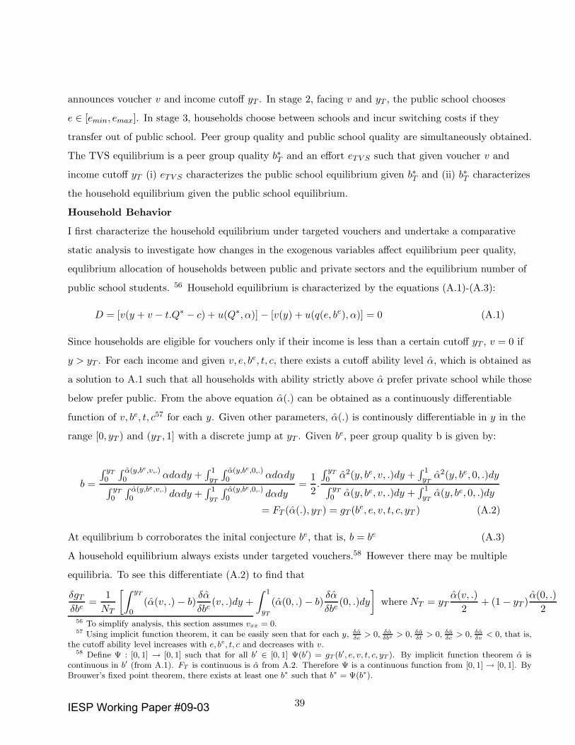
announces voucher v and income cutoff yT . In stage 2, facing v and yT , the public school chooses
e ∈ [emin, emax]. In stage 3, households choose between schools and incur switching costs if they
transfer out of public school. Peer group quality and public school quality are simultaneously obtained.
The TVS equilibrium is a peer group quality b∗T and an effort eTV S such that given voucher v and
income cutoff yT (i) eTV S characterizes the public school equilibrium given b∗T and (ii) b∗T characterizes
the household equilibrium given the public school equilibrium.
Household Behavior
I first characterize the household equilibrium under targeted vouchers and undertake a comparative
static analysis to investigate how changes in the exogenous variables affect equilibrium peer quality,
equlibrium allocation of households between public and private sectors and the equilibrium number of
public school students. 56 Household equilibrium is characterized by the equations (A.1)-(A.3):
D = [v(y + v − t.Q∗ − c) + u(Q∗, α)] − [v(y) + u(q(e, be), α)] = 0 (A.1)
Since households are eligible for vouchers only if their income is less than a certain cutoff yT , v = 0 if
y > yT . For each income and given v, e, be, t, c, there exists a cutoff ability level α, which is obtained as
a solution to A.1 such that all households with ability strictly above α prefer private school while those
below prefer public. From the above equation α(.) can be obtained as a continuously differentiable
function of v, be, t, c57 for each y. Given other parameters, α(.) is continously differentiable in y in the
range [0, yT ) and (yT , 1] with a discrete jump at yT . Given be, peer group quality b is given by:
b =
∫ yT
0
∫ α(y,be,v,.)0 αdαdy +
∫ 1yT
∫ α(y,be,0,.)0 αdαdy
∫ yT
0
∫ α(y,be,v,.)0 dαdy +
∫ 1yT
∫ α(y,be,0,.)0 dαdy
=1
2.
∫ yT
0 α2(y, be, v, .)dy +∫ 1yT
α2(y, be, 0, .)dy∫ yT
0 α(y, be, v, .)dy +∫ 1yT
α(y, be, 0, .)dy
= FT (α(.), yT ) = gT (be, e, v, t, c, yT ) (A.2)
At equilibrium b corroborates the inital conjecture be, that is, b = be (A.3)
A household equilibrium always exists under targeted vouchers.58 However there may be multiple
equilibria. To see this differentiate (A.2) to find that
δgT
δbe=
1
NT
[∫ yT
0(α(v, .) − b)
δα
δbe(v, .)dy +
∫ 1
yT
(α(0, .) − b)δα
δbe(0, .)dy
]
where NT = yTα(v, .)
2+ (1 − yT )
α(0, .)
256 To simplify analysis, this section assumes vxx = 0.57 Using implicit function theorem, it can be easily seen that for each y, δα
δe> 0, δα
δbe > 0, δαδt
> 0, δαδc
> 0, δαδv
< 0, that is,the cutoff ability level increases with e, be, t, c and decreases with v.
58 Define Ψ : [0, 1] → [0, 1] such that for all b′ ∈ [0, 1] Ψ(b′) = gT (b′, e, v, t, c, yT ). By implicit function theorem α iscontinuous in b′ (from A.1). FT is continuous is α from A.2. Therefore Ψ is a continuous function from [0, 1] → [0, 1]. ByBrouwer’s fixed point theorem, there exists at least one b∗ such that b∗ = Ψ(b∗).
39IESP Working Paper #09-03

The sign of δgT
δbe is positive.59 If it exceeds one, there may be multiple equilibria. Parameter values such
that b(0) > 0 and δgT
δbe < 1 ensure a unique equilibrium. While 0 < α < 1 ensures b(0) > 0, the second
condition holds if the marginal utility from school quality and the marginal responsiveness of public
school quality to peer quality are not too high.
Lemma A.1 Under targeted vouchers, peer group quality falls with vouchers and increases with public
school effort.
Lemma A.2 Under targeted vouchers, an increase in public school effort leads to reverse sorting by
both income and ability. Targeted vouchers increase sorting by income and ability.60
Proposition A.1 Equilibrium number of public school students decreases with targeted vouchers and
increases with public school effort under targeted vouchers.
The intuition behind lemmas A.1 and A.2 and proposition A.1 are exactly the same as earlier.
However, since vouchers are targeted here only to the low income population, high ability households
only at each income level less than or equal to yT switch to private schools with vouchers. An increase
in effort however leads to an influx of high ability households at each income level similar to that in the
universal vouchers case.
Lemma A.3 Given e, v, t, c, equilibrium number of public school students under targeted vouchers is
greater than that under a universal vouchers system.
Universal vouchers lead to a switch of high ability households at each income level whereas targeted
vouchers leads to a flight of high ability households only for income levels less than or equal to yT .
Therefore loss of students due to vouchers is greater under the universal than the targeted regime,
given all other parameters.
Public School Behavior
The public school correctly anticipates household behavior under targeted vouchers and chooses effort
to maximize its rent RT (e, v) = pNT (e, v) − c(NT (e, v)) − C(e). There exists a unique effort eTV S that
solves its first order condition δRT (e,v)δe
= (p − cNT) δNT (e,v)
δe− Ce(e) = 0. Since the imposition of
targeted vouchers also leads to a flight of households from public school, it leads to a fall in public
school rent.61 Equilibrium public school effort under the TVS equilibrium can be either greater or less
59 The proof is in appendix E. All proofs for this section are in appendix E.60 The proof follows on the same lines as above and hence is skipped.61 δRT (e,v)
δv= (p− cNT
) δNT (e,v)δv
which is negative because δNT
δv< 0 by proposition A.1 and (p− cNT
) > 0 by assumption.
40IESP Working Paper #09-03
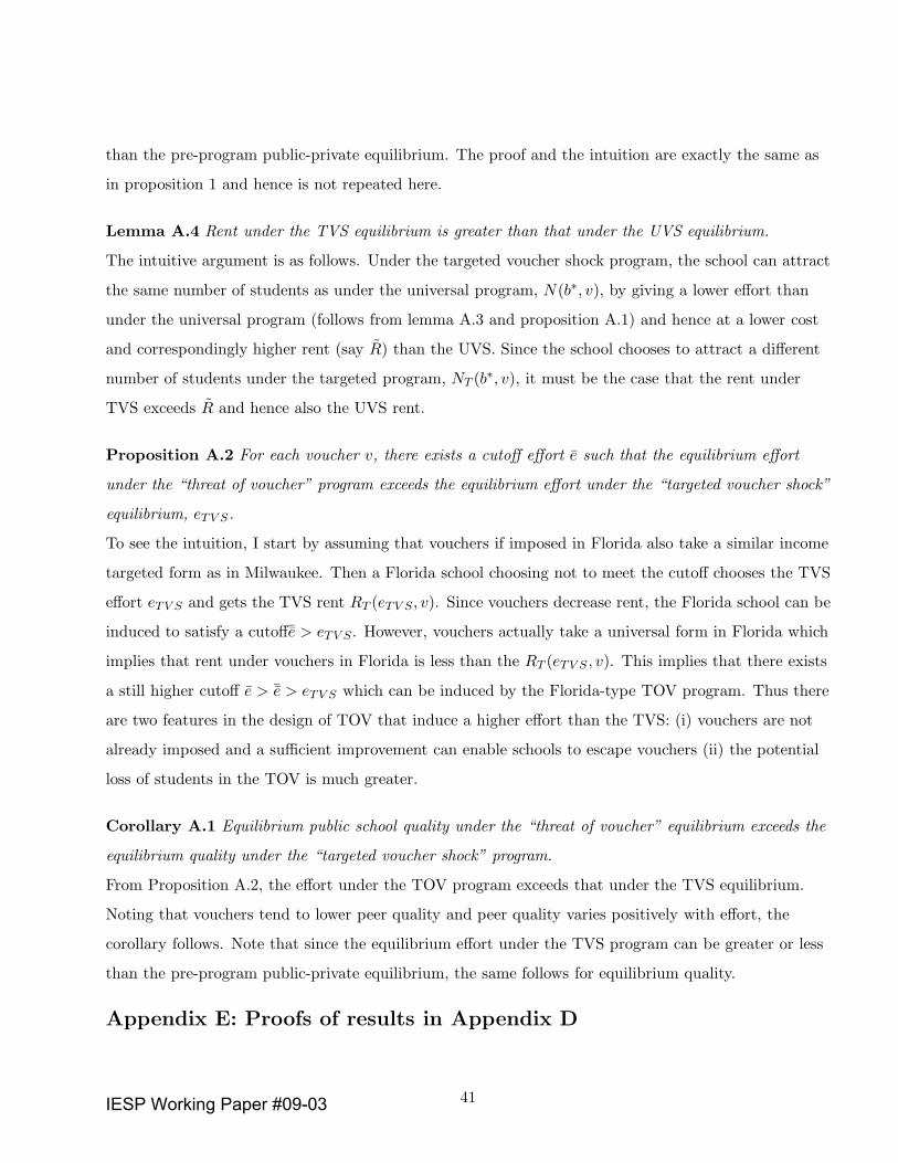
than the pre-program public-private equilibrium. The proof and the intuition are exactly the same as
in proposition 1 and hence is not repeated here.
Lemma A.4 Rent under the TVS equilibrium is greater than that under the UVS equilibrium.
The intuitive argument is as follows. Under the targeted voucher shock program, the school can attract
the same number of students as under the universal program, N(b∗, v), by giving a lower effort than
under the universal program (follows from lemma A.3 and proposition A.1) and hence at a lower cost
and correspondingly higher rent (say R) than the UVS. Since the school chooses to attract a different
number of students under the targeted program, NT (b∗, v), it must be the case that the rent under
TVS exceeds R and hence also the UVS rent.
Proposition A.2 For each voucher v, there exists a cutoff effort e such that the equilibrium effort
under the “threat of voucher” program exceeds the equilibrium effort under the “targeted voucher shock”
equilibrium, eTV S.
To see the intuition, I start by assuming that vouchers if imposed in Florida also take a similar income
targeted form as in Milwaukee. Then a Florida school choosing not to meet the cutoff chooses the TVS
effort eTV S and gets the TVS rent RT (eTV S, v). Since vouchers decrease rent, the Florida school can be
induced to satisfy a cutoff¯e > eTV S . However, vouchers actually take a universal form in Florida which
implies that rent under vouchers in Florida is less than the RT (eTV S , v). This implies that there exists
a still higher cutoff e > ¯e > eTV S which can be induced by the Florida-type TOV program. Thus there
are two features in the design of TOV that induce a higher effort than the TVS: (i) vouchers are not
already imposed and a sufficient improvement can enable schools to escape vouchers (ii) the potential
loss of students in the TOV is much greater.
Corollary A.1 Equilibrium public school quality under the “threat of voucher” equilibrium exceeds the
equilibrium quality under the “targeted voucher shock” program.
From Proposition A.2, the effort under the TOV program exceeds that under the TVS equilibrium.
Noting that vouchers tend to lower peer quality and peer quality varies positively with effort, the
corollary follows. Note that since the equilibrium effort under the TVS program can be greater or less
than the pre-program public-private equilibrium, the same follows for equilibrium quality.
Appendix E: Proofs of results in Appendix D
41IESP Working Paper #09-03

Proof of δgT
δbe > 0 :
δgT
δbe=
1
NT
[∫ yT
0(α(v, .) − b)
δα
δbe(v, .)dy +
∫ 1
yT
(α(0, .) − b)δα
δbe(0, .)dy
]
where NT = yTα(v, .)
2+ (1 − yT )
α(0, .)
2.
The proof consists of the following steps:
(i)∫ 10 αdy − b is positive.
Noting that b = yT
NT
∫ α(v,.)0 αdα + (1−yT )
NT
∫ α(0,.)0 αdα, it follows that
∫ 10 αdy − b = yT [α(v, .) −
∫ α(v,.)0NT
] + (1 − yT )[α(0, .) −∫ α(0,.)0NT
]. Since the expression in each of the square
brackets is positive,∫ 10 αdy − b is positive.
(ii) α(v,.)2 < b < α(0,.)
2 .
From above, b = yT α(v)NT
α(v,.)2 + (1−yT )α(0,.)
NT
α(0,.)2 Therefore b is a weighted average of α(v,.)
2 and α(0,.)2 .
(iii) Now,
δgT
δbe=
1
NT
[yT (α(v, .) − b)δα
δbe(v, .)dy + (1 − yT )(α(0, .) − b)
δα
δbe(0, .)dy]
There are two possible cases:
Case (a): b < α(v, .) < α(0, .). Then it follows that δgT
δbe > 0.
Case (b): α(v, .) < b < α(0, .).
Now,∫ 10 α(.)dy − b > 0 ⇒ yT α(v, .) + (1− yT )α(0, .) − b > 0 ⇒ yT [α(v, .) − b] + (1− yT )[α(0, .) − b] > 0.
Then it must be the case that (1 − yT )[α(0, .) − b] > |yT [α(v, .) − b]|. Using equation A.1, it can be
easily seen that δ2αδvδbe =
uqαbe
δαδv
uQα−u
qα
< 0. It follows therefore that
(1 − yT )[α(0, .) − b] δαδbe (0, .) >
∣
∣yT [α(v, .) − b] δαδbe (v, .)
∣
∣. Hence δgT
δbe > 0.
Proof of Lemma A.1. At the household equilibrium under targeted vouchers,
b∗T = gT (b∗T , e, v, t, c, yT ) where b∗T denotes the equilibrium peer quality under targeted vouchers.
Effect of an increase in e:
δb∗Tδe
=
δgT (b∗T ,.)δe
1 −δgT (b∗
T,.)
δb
where,
The denominator is positive from the uniqueness condition. Consider the numerator.
δgT (b∗T , .)
δe=
1
NT (b∗T , .)
[∫ yT
0(α(v, b∗T , .) − b∗T ).
δα(v, b∗T , .)
δedy +
∫ 1
yT
(α(0) − b∗T )δα(0, b∗T , .)
δedy
]
=1
NT (b∗T , .)
[
yT (α(v, b∗T , .) − b∗T ).δα(v, b∗T , .)
δe+ (1 − yT )(α(0) − b∗T )
δα(0, b∗T , .)
δe
]
42IESP Working Paper #09-03

The second line follows because vxx = 0. Using equation A.1, δ2αδvδe
=u
qαe. δα
δv
uQα−u
qα
, which is negative.
Therefore, it follows from the proof of δgT
δbe > 0 thatδgT (b∗T ,.)
δe> 0.
Effect of an increase in v:
δb∗Tδv
=
δgT (b∗T ,.)δv
1 −δgT (b∗
T,.)
δb
where,
δgT (b∗T , v, .)
δv=
1
NT
[∫ yT
0(α(v, .) − b∗T ).
δα(v, b∗T , .)
δvdy
]
Starting from a status quo position of v = 0 consider a marginal increase in v targeted to low income
households with y ≤ yT . The denominator is positive. Consider the numerator.
δgT (b∗T (0), 0, .)
δv=
1
NT
[∫ yT
0(α(0, .) − b∗T (0))
δα(0, .)
δvdy
]
=1
NTyT (α(0, .) − b∗T (0))
δα(0, .)
δv
Note that∫ 10 (α(0) − b∗T (0)) = (α(0) − b∗T (0)) > 062 since b∗T (0) = α(0)
2 . It follows thatδgT (b∗
T,0,.)
δv< 0.
Proof of Proposition A.1. Noting that NT (e, v, .) =∫ yT
0 α(e, v, .)dy +∫ 1yT
α(e, 0, .)dy, the proof
follows from lemma A.2.
Proof of Lemma A.3.
N(e, v, .) =
∫ yT
0
∫ α(y,e,v,.)
0dαdy +
∫ 1
yT
∫ α(y,e,v,.)
0dαdy <
∫ yT
0
∫ α(y,e,v,.)
0dαdy +
∫ 1
yT
∫ α(y,e,0,.)
0dαdy = NT (e, v, .)
The inequality follows from lemma A.2.
Proof of Lemma A.4. At the UVS equilibrium, the school chooses eV S, attracts N(eV S , v) and earns
rent pN(eV S , v) − c(N(eV S , v)) − C(e). Now NT (eV S , v) > N(eV S, v), (from lemma A.3). Therefore
given v, ∃e < eV S such that NT (e, v) = N(eV S, v), since δNT
δe> 0. Then,
R(eV S , v) = pN(eV S, v) − c(N(eV S, v)) − C(e) < pNT (e, v) − c(NT (e, v)) − C(e)
< pNT (eTV S , v) − c(NT (eTV S , v)) − C(eTV S) = RT (eTV S , v)
The first inequality follows because a lower effort generates smaller costs and hence higher rent, given
revenue. The second inequality follows because eTV S is the rent maximizing effort under targeted
vouchers.
Proof of Proposition A.2.
The proof consists of two steps:
62 When v = 0, b∗T (0) is the same as b∗(0).
43IESP Working Paper #09-03

Step 1: First assume that vouchers, if imposed under the TOV program, take a similar targeted form
as in the TVS case. Then if the school decides not to meet the cutoff, it chooses eTV S and gets the
TVS equilibrium rent. Since vouchers decrease rent:
pN(eTV S , 0) − c(N(eTV S , 0)) − C(eTV S) > pNT (eTV S , v) − c(NT (eTV S , v)) − C(eTV S) = RT (eTV S , v)
Therefore, ∃ ¯e > eTV S such that the public school incentive constraint is satisfied with equality.
Step 2: However, since vouchers under the TOV program actually take the universal form rather than
the targeted form, school chooses eV S and gets rent R(eV S , v) if it fails to meet the cutoff. Then it
follows from step 1 and lemma A.4:
R(¯e, 0) = RT (eTV S , v) > R(eV S , v)
Therefore ∃e > ¯e > eTV S such that R(e, 0) = R(eV S , v).
Proof of Corollary A.1. eTOV > eTV S from proposition A.2
⇒ q(eTOV , b∗(eTOV , 0)) > q(eTV S , b∗T (eTV S , 0)) > q(eTV S , b∗T (eTV S , v)) since qe, qb > 0 and
δb∗T
δe> 0,
δb∗T
δv< 0.
References
Angrist Joshua D., and Victor Lavy (1999), “Using Maimonides’ Rule to Estimate the Effect of
Class Size on Scholastic Achievement,” Quarterly Journal of Economics 114(2), 533-575.
Camilli, Gregory and Bulkley, Katrina (2001), “Critique of ‘An Evaluation of the Florida A-Plus
Accountability and School Choice Program’,” Education Policy Analysis Archives, Vol. 9, Number 7.
Caucutt, Elizabeth (2002), “Educational Vouchers when there are Peer Group Effects-Size Matters”
International Economic Review, 43(1), 195-222.
Chen, Zhiqi and Edwin G. West (2000), “Selective Versus Universal Vouchers: Modeling Median
voter Preferences in Education,” American Economic Review, 90(5), 1520-1534.
Chakrabarti, Rajashri (2004),“Can Increasing Private School Participation in a Voucher Program
Affect Public School Performance? Evidence from the Milwaukee Voucher Experiment,” mimeo,
Harvard University.
Chakrabarti, Rajashri (2005),“Do Vouchers Lead to Sorting Even Under Random Private School
Selection? Evidence from Milwaukee ,” mimeo, Harvard University.
Chay, Kenneth, Patrick McEwan and Miguel Urquiola (2003), “The central role of noise in
evaluating interventions that use test scores to rank schools,” NBER Working Paper # 9354.
44IESP Working Paper #09-03

Epple, Dennis and Richard Romano (1998), “Competition between Private and Public Schools,
Vouchers and Peer Group Effects,” American Economic Review 62(1), 33-62.
Epple, Dennis and Richard Romano (2002), “Educational Vouchers and Cream Skimming”
NBER Working Paper # 9354.
Figlio, David and Maurice E. Lucas (2004),“What’s in a Grade? School Report Cards and the
Housing Market,” American Economic Review 94(3), 591-604.
Figlio, David and Cecilia Rouse (2004), “Do Accountability and Voucher Threats Improve
Low-Performing Schools?”, mimeo, University of Florida and Princeton University.
Greene, Jay (2001), “An Evaluation of the Florida A-Plus Accountability and School Choice
Program,” New York: Manhattan Institute for Policy Research.
Greene, Jay P. and Marcus A. Winters (2003), “When Schools Compete: The Effects of Vouchers
on Florida Public School Achievement,” Education Working Paper 2.
Hahn, J., P. Todd, and W. Van der Klaauw (2001), “Identification and Estimation of Treatment
Effects with a Regression-Discontinuity Design,” Econometrica 69 (2001), 201-209.
Hanushek, Eric A. and Margaret E. Raymond (2003), “Improving Educational Quality: How
Best to Judge Our Schools?” in Yolanda Kodrzycki (ed.) Education in the 21st Century: Meeting the
Challenges of a Changing World, Federal Reserve Bank of Boston, 193-224.
Harris, Doug (2001), “What Caused the Effects of the Florida A+ Program: Ratings or Vouchers?”
in Martin Carnoy (ed.), School Vouchers: Examining the Evidence, Economic Policy Institute.
Hoxby, Caroline (2001), “Ideal Vouchers”, Harvard University typescript.
Hoxby, Caroline M. (2003a), “School Choice and School Productivity (Or, Could School Choice be
the tide that lifts all boats?)”, in C. Hoxby ed. The Economics of School Choice, University of Chicago
Press.
Hoxby, Caroline (2003b), “School Choice and School Competition: Evidence from the United
States”, Swedish Economic Policy Review.
Hoyt, William and Kangoh Lee (1998), “Educational vouchers, Welfare Effects and Voting,”
Journal of Public Economics, 69, 211-228.
Hsieh Chang-Tai and Miguel Urquiola (2003), “ When Schools Compete, how do they Compete?
An assessment of Chile’s nationwide School Voucher Program,” NBER Working Paper # 10008.
Innerst, Carol (2000), “Competing to win: How Florida’s A-Plan has Triggered Public School
Reform,” Urban League of Greater Miami, The Collins Center for Public Policy, Floridians for School
45IESP Working Paper #09-03

Choice, the James Madison Institute and the Center for education Reform.
Jacob, Brian A., and Lans Lefgren (2004a), “Remedial Education and Student Achievement: A
Regression-Discontinuity Analysis,” Review of Economics and Statistics LXXXVI(1).
Jacob, Brian A., and Lans Lefgren (2004b), “The Impact of Teacher Training on Student
Achievement: Quasi- Experimental Evidence from School Reform Efforts in Chicago,” Journal of
Human Resources 39(1).
Kupermintz, Haggai (2001), “The Effects of vouchers on School Improvement: Another Look at the
Florida Data”, Education Policy Analysis Archives, Volume 9, Number 8.
McMillan, Robert (2004),“Competition, Incentives, and Public School Productivity,” Journal of Pub-
lic Economics, 88, 1871-1892.
Manski, Charles F. (1992), “Educational Choice (Vouchers) and Social Mobility,” Economics of Ed-
ucation Review, 11(4), 531-542.
Nechyba, Thomas J. (1996), “Public School Finance in a General Equilibrium Tiebout World: Equal-
ization Programs, Peer Effects and Private School Vouchers,” NBER working paper # 5642.
Nechyba, Thomas J. (1999), “School Finance Induced Migration Patterns: The case of Private School
Vouchers,” Journal of Public Economic Theory 1 (1), 5-50.
Nechyba, Thomas J. (2000), “Mobility, Targeting, and Private-School Vouchers”, American Economic
Review 90(1), 130-146.
Nechyba, Thomas J. (2003), “Introducing School Choice into Multi-District Public School Systems”,
in Caroline Hoxby (ed.), The Economics of School Choice, University of Chicago Press, Chicago.
Rouse, Cecilia E. (1998), “Private School Vouchers and Student Achievement: Evidence from the
Milwaukee Choice Program,” Quarterly Journal of Economics 113(2), 553-602.
Van der Klaauw, W. (2002), Estimating the Effect of Financial Aid Offers on College Enrollment: A
Regression-Discontinuity Approach,” International Economic Review 43(4), 2002, 1249-1287.
West, Martin and Paul Peterson (2005), “The Efficacy of Choice Threats within School Account-
ability Systems: Results from Legislatively Induced Experiments”, Harvard University, Program on
Education Policy and Governance, PEPG # 05-01.
Witte, John F. (2000), “The Market Approach to Education: An analysis of America’s First Voucher
Program,” Princeton University Press, Princeton.
46IESP Working Paper #09-03
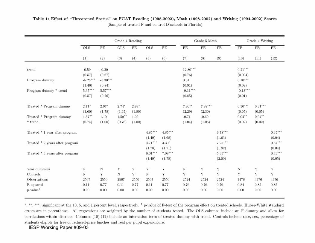
Table 1: Effect of “Threatened Status” on FCAT Reading (1998-2002), Math (1998-2002) and Writing (1994-2002) Scores
(Sample of treated F and control D schools in Florida)
Grade 4 Reading Grade 5 Math Grade 4 Writing
OLS FE OLS FE OLS FE FE FE FE FE FE FE
(1) (2) (3) (4) (5) (6) (7) (8) (9) (10) (11) (12)
trend -0.59 -0.20 12.80∗∗∗ 0.21∗∗∗
(0.57) (0.67) (0.76) (0.004)
Program dummy -5.25∗∗∗ -5.30∗∗∗ 0.31 0.10∗∗∗
(1.46) (0.84) (0.91) (0.02)
Program dummy * trend 5.35∗∗∗ 5.57∗∗∗ -9.11∗∗∗ -0.13∗∗∗
(0.57) (0.76) (0.85) (0.01)
Treated * Program dummy 2.71∗ 2.97∗ 2.74∗ 2.99∗ 7.90∗∗ 7.88∗∗∗ 0.30∗∗∗ 0.31∗∗∗
(1.60) (1.78) (1.65) (1.80) (2.29) (2.30) (0.05) (0.05)
Treated * Program dummy 1.57∗∗ 1.10 1.59∗∗ 1.09 -0.71 -0.60 0.04∗∗ 0.04∗∗
* trend (0.74) (1.00) (0.76) (1.00) (1.04) (1.06) (0.02) (0.02)
Treated * 1 year after program 4.85∗∗∗ 4.85∗∗∗ 6.78∗∗∗ 0.35∗∗∗
(1.49) (1.68) (1.63) (0.04)
Treated * 2 years after program 4.71∗∗∗ 3.30∗ 7.25∗∗∗ 0.37∗∗∗
(1.78) (1.71) (1.82) (0.04)
Treated * 3 years after program 8.01∗∗∗ 7.08∗∗∗ 5.35∗∗∗ 0.43∗∗∗
(1.49) (1.78) (2.00) (0.05)
Year dummies N N Y Y Y Y N Y Y N Y Y
Controls N Y N Y N Y Y Y Y Y Y Y
Observations 2567 2550 2567 2550 2567 2550 2524 2524 2524 4476 4476 4476
R-squared 0.11 0.77 0.11 0.77 0.11 0.77 0.76 0.76 0.76 0.84 0.85 0.85
p-value1 0.00 0.00 0.00 0.00 0.00 0.00 0.00 0.00 0.00 0.00 0.00 0.00
∗, ∗∗, ∗∗∗: significant at the 10, 5, and 1 percent level, respectively. 1 p-value of F-test of the program effect on treated schools. Huber-White standard
errors are in parentheses. All regressions are weighted by the number of students tested. The OLS columns include an F dummy and allow for
correlations within districts. Columns (10)-(12) include an interaction term of treated dummy with trend. Controls include race, sex, percentage of
students eligible for free or reduced-price lunches and real per pupil expenditure.
IESP Working Paper #09-03
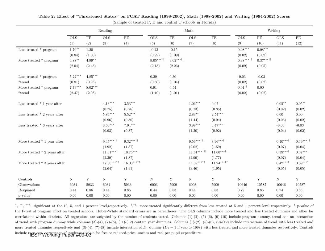
Table 2: Effect of “Threatened Status” on FCAT Reading (1998-2002), Math (1998-2002) and Writing (1994-2002) Scores
(Sample of treated F, D and control C schools in Florida)
Reading Math Writing
OLS FE OLS FE OLS FE OLS FE OLS FE OLS FE
(1) (2) (3) (4) (5) (6) (7) (8) (9) (10) (11) (12)
Less treated * program 1.70∗∗ 1.20 -0.23 -0.15 0.08∗∗∗ 0.08∗∗∗
(0.84) (1.00) (0.92) (1.09) (0.02) (0.02)
More treated * program 4.88∗∗ 4.99∗∗ 9.05∗∗∗†† 9.02∗∗∗†† 0.38∗∗∗†† 0.37∗∗∗††
(2.04) (2.43) (2.13) (2.23) (0.09) (0.05)
Less treated * program 5.22∗∗∗ 4.85∗∗∗ 0.29 0.30 -0.03 -0.03
*trend (0.81) (0.93) (0.60) (1.04) (0.02) (0.02)
More treated * program 7.73∗∗∗ 8.02∗∗∗ 0.91 0.54 0.01†† 0.00
*trend (2.47) (2.08) (1.10) (1.01) (0.02) (0.02)
Less treated * 1 year after 4.13∗∗∗ 3.53∗∗∗ 1.06∗∗∗ 0.97 0.05∗∗ 0.05∗∗
(0.75) (0.76) (0.73) (0.85) (0.02) (0.02)
Less treated * 2 years after 5.84∗∗∗ 5.52∗∗∗ 2.83∗∗ 2.54∗∗∗ 0.00 0.00
(0.96) (0.80) (1.44) (0.94) (0.03) (0.02)
Less treated * 3 years after 8.60∗∗∗ 7.94∗∗∗ 3.89∗∗∗ 3.47∗∗∗ -0.03 -0.03
(0.93) (0.87) (1.20) (0.92) (0.04) (0.02)
More treated * 1 year after 9.45∗∗∗†† 9.32∗∗∗†† 9.56∗∗∗†† 8.96∗∗∗†† 0.40∗∗∗†† 0.39∗∗∗††
(1.92) (1.87) (2.02) (1.59) (0.07) (0.04)
More treated * 2 years after 11.01∗∗∗† 10.75∗∗∗† 11.61∗∗∗††† 11.00∗∗∗†† 0.39∗∗∗† 0.37∗∗∗†
(2.39) (1.87) (2.99) (1.77) (0.07) (0.04)
More treated * 3 years after 17.08∗∗∗†† 16.03∗∗∗†† 11.39∗∗∗†† 11.94∗∗∗†† 0.42∗∗∗† 0.39∗∗∗†
(2.64) (1.91) (3.46) (1.95) (0.05) (0.05)
Controls N Y N Y N Y N Y N Y N Y
Observations 6034 5933 6034 5933 6003 5909 6003 5909 10646 10587 10646 10587
R-squared 0.44 0.86 0.44 0.86 0.44 0.83 0.44 0.83 0.72 0.85 0.74 0.86
p-value1 0.00 0.00 0.00 0.00 0.00 0.00 0.00 0.00 0.00 0.00 0.00 0.00
∗, ∗∗, ∗∗∗: significant at the 10, 5, and 1 percent level,respectively. †,††: more treated significantly different from less treated at 5 and 1 percent level respectively. 1 p-value of
the F-test of program effect on treated schools. Huber-White standard errors are in parentheses. The OLS columns include more treated and less treated dummies and allow for
correlations within districts. All regressions are weighted by the number of students tested. Columns (1)-(2), (5)-(6), (9)-(10) include program dummy, trend and an interaction
of trend with program dummy while columns (3)-(4), (7)-(8), (11)-(12) contain year dummies. Columns (1)-(2), (5)-(6), (9)-(12) include interactions of trend with less treated and
more treated dummies respectively and (3)-(4), (7)-(8) include interaction of D1 dummy (D1 = 1 if year > 1998) with less treated and more treated dummies respectively. Controls
include race, sex, percentage of students eligible for free or reduced-price lunches and real per pupil expenditure.IESP Working Paper #09-03

Table 3: Effect of the Milwaukee “Voucher Shock” Program
Using treatment groups Cont. treatment var.
WRCT (% above) ITBS Reading ITBS Math WRCT (% above)
(1) (2) (3) (4) (5) (6) (7)
Somewhat treated*program dummy 3.50 3.57 0.39
(2.59) (5.24) (2.81)
More treated * program dummy 2.85 1.61 -2.97
(3.32) (4.98) (3.13)
Somewhat treated*program dummy 0.64 1.34 0.61
*trend (0.47) (0.34) (0.54)
More treated*program dummy*trend 0.67 0.94 0.50
(0.62) (2.31) (0.63)
Somewhat treated * 1 year after program 2.03 4.15 -1.35
(2.81) (4.49) (2.94)
Somewhat treated * 2 years after program 5.38∗∗ 7.83 6.14∗
(2.43) (5.17) (3.38)
Somewhat treated * 3 years after program 5.01 6.78 2.47
(3.03) (5.31) (3.31)
More treated * 1 year after program -0.92 1.12 -4.02
(3.33) (3.86) (3.26)
More treated * 2 years after program 6.06∗ 6.59 4.36
(3.14) (5.15) (3.83)
More treated * 3 years after program 5.69 2.85 -2.22
(3.98) (5.18) (3.54)
Treatment * 1 year after program -0.09
( 0.09)
Treatment * 2 years after program 0.07
(0.09)
Treatment * 3 years after program 0.03
(0.11)
Year dummies N Y N Y N Y Y
Observations 1195 1195 717 717 1127 1127 920
R-squared 0.50 0.58 0.55 0.55 0.58 0.60 0.55
p-value1 0.06 0.11 0.67 0.62 0.49 0.27 0.29
∗, ∗∗, ∗∗∗: significant at the 10, 5, and 1 percent level, respectively. 1 p-value of the F-test of joint significance of
more treated shift coefficients. Huber-White standard errors are in parentheses. This table uses the 66-47 sample. All
regressions include school fixed effects and control for race, sex, percentage of students eligible for free or reduced-price
lunches and real per pupil expenditure. Columns (1), (3), (5) include program dummy, trend and an interaction of
trend with program dummy.
IESP Working Paper #09-03
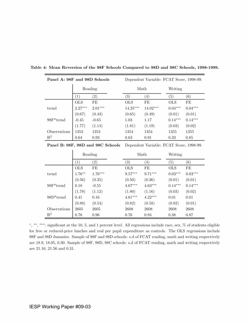
Table 4: Mean Reversion of the 98F Schools Compared to 98D and 98C Schools, 1998-1999.
Panel A: 98F and 98D Schools Dependent Variable: FCAT Score, 1998-99.
Reading Math Writing
(1) (2) (3) (4) (5) (6)
OLS FE OLS FE OLS FE
trend 2.27∗∗∗ 2.01∗∗∗ 14.25∗∗∗ 14.02∗∗∗ 0.04∗∗∗ 0.04∗∗∗
(0.67) (0.43) (0.65) (0.49) (0.01) (0.01)
98F*trend -0.45 -0.65 1.03 1.17 0.14∗∗∗ 0.14∗∗∗
(1.77) (1.14) (1.81) (1.19) (0.03) (0.02)
Observations 1353 1353 1354 1354 1355 1355
R2 0.64 0.93 0.63 0.91 0.33 0.85
Panel B: 98F, 98D and 98C Schools Dependent Variable: FCAT Score, 1998-99.
Reading Math Writing
(1) (2) (3) (4) (5) (6)
OLS FE OLS FE OLS FE
trend 1.76∗∗ 1.76∗∗∗ 9.57∗∗∗ 9.71∗∗∗ 0.03∗∗∗ 0.03∗∗∗
(0.56) (0.35) (0.50) (0.36) (0.01) (0.01)
98F*trend 0.18 -0.55 4.67∗∗∗ 4.63∗∗∗ 0.14∗∗∗ 0.14∗∗∗
(1.78) (1.12) (1.80) (1.16) (0.03) (0.02)
98D*trend 0.41 0.16 4.61∗∗∗ 4.22∗∗∗ 0.01 0.01
(0.88) (0.54) (0.82) (0.58) (0.02) (0.01)
Observations 2605 2605 2608 2608 2608 2608
R2 0.76 0.96 0.76 0.94 0.38 0.87
∗, ∗∗, ∗∗∗: significant at the 10, 5, and 1 percent level. All regressions include race, sex, % of students eligible
for free or reduced-price lunches and real per pupil expenditure as controls. The OLS regressions include
98F and 98D dummies. Sample of 98F and 98D schools: s.d of FCAT reading, math and writing respectively
are 18.9, 18.05, 0.30. Sample of 98F, 98D, 98C schools: s.d of FCAT reading, math and writing respectively
are 21.16, 21.56 and 0.31.
IESP Working Paper #09-03
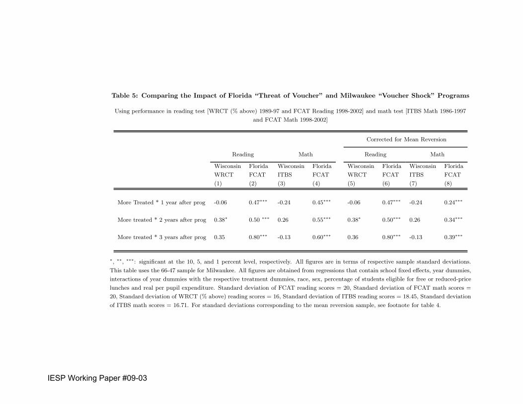
Table 5: Comparing the Impact of Florida “Threat of Voucher” and Milwaukee “Voucher Shock” Programs
Using performance in reading test [WRCT (% above) 1989-97 and FCAT Reading 1998-2002] and math test [ITBS Math 1986-1997
and FCAT Math 1998-2002]
Corrected for Mean Reversion
Reading Math Reading Math
Wisconsin Florida Wisconsin Florida Wisconsin Florida Wisconsin Florida
WRCT FCAT ITBS FCAT WRCT FCAT ITBS FCAT
(1) (2) (3) (4) (5) (6) (7) (8)
More Treated * 1 year after prog -0.06 0.47∗∗∗ -0.24 0.45∗∗∗ -0.06 0.47∗∗∗ -0.24 0.24∗∗∗
More treated * 2 years after prog 0.38∗ 0.50 ∗∗∗ 0.26 0.55∗∗∗ 0.38∗ 0.50∗∗∗ 0.26 0.34∗∗∗
More treated * 3 years after prog 0.35 0.80∗∗∗ -0.13 0.60∗∗∗ 0.36 0.80∗∗∗ -0.13 0.39∗∗∗
∗, ∗∗, ∗∗∗: significant at the 10, 5, and 1 percent level, respectively. All figures are in terms of respective sample standard deviations.
This table uses the 66-47 sample for Milwaukee. All figures are obtained from regressions that contain school fixed effects, year dummies,
interactions of year dummies with the respective treatment dummies, race, sex, percentage of students eligible for free or reduced-price
lunches and real per pupil expenditure. Standard deviation of FCAT reading scores = 20, Standard deviation of FCAT math scores =
20, Standard deviation of WRCT (% above) reading scores = 16, Standard deviation of ITBS reading scores = 18.45, Standard deviation
of ITBS math scores = 16.71. For standard deviations corresponding to the mean reversion sample, see footnote for table 4.
IESP Working Paper #09-03

Table 6A: Pre-program Characteristics of Florida F and D schools
in Regression Discontinuity Sample
F D F-D
(std. dev.) (std. dev.) [p-value]
% black 64.68 64.08 0.60
(28.39) (28.18) [0.92]
% hispanic 17.99 20.16 -2.16
(20.88) (23.67) [0.66]
% white 16.42 14.31 2.11
(18.81) (16.83) [0.57]
% male 51.22 51.49 -0.27
(4.00) (5.43) [0.81]
% free-reduced lunch 86.30 83.60 2.64
(8.34) (11.98) [0.26]
FCAT Reading Score 253.97 254.18 -0.21
(17.33) (15.47) [0.95]
FCAT Math Score 274.25 275.64 -1.39
(13.34) (13.49) [0.63]
FCAT Writing Score 2.55 2.68 -0.02
(0.11) (0.11) [0.00]
Number of Schools 33 70
Table 6B: Regression Discontinuity Analysis in Florida
Reading Math Writing
FE FE FE
(1) (2) (3)
Treated * 1 year after Program 4.21∗ 8.03∗∗∗ 0.19∗∗∗
(2.46) (2.58) (0.06)
Treated * 2 years after Program 3.45∗ 7.12∗∗ 0.12∗
(2.06) (3.04) (0.06)
Treated * 3 years after Program 7.47∗∗ 6.49∗∗ 0.20∗∗∗
(3.06) (3.26) (0.08)
Year dummies Y Y Y
Observations 513 505 909
R-squared 0.76 0.76 0.87
p-value 0.01 0.00 0.00
∗, ∗∗, ∗∗∗ denote significance at the 10, 5, and 1 percent levels respectively. Huber-White standard errors are in
parentheses. All regressions are weighted by the number of students tested, include school fixed effects and control
for race, sex, percentage of students eligible for free or reduced price lunches and real per pupil expenditure.IESP Working Paper #09-03
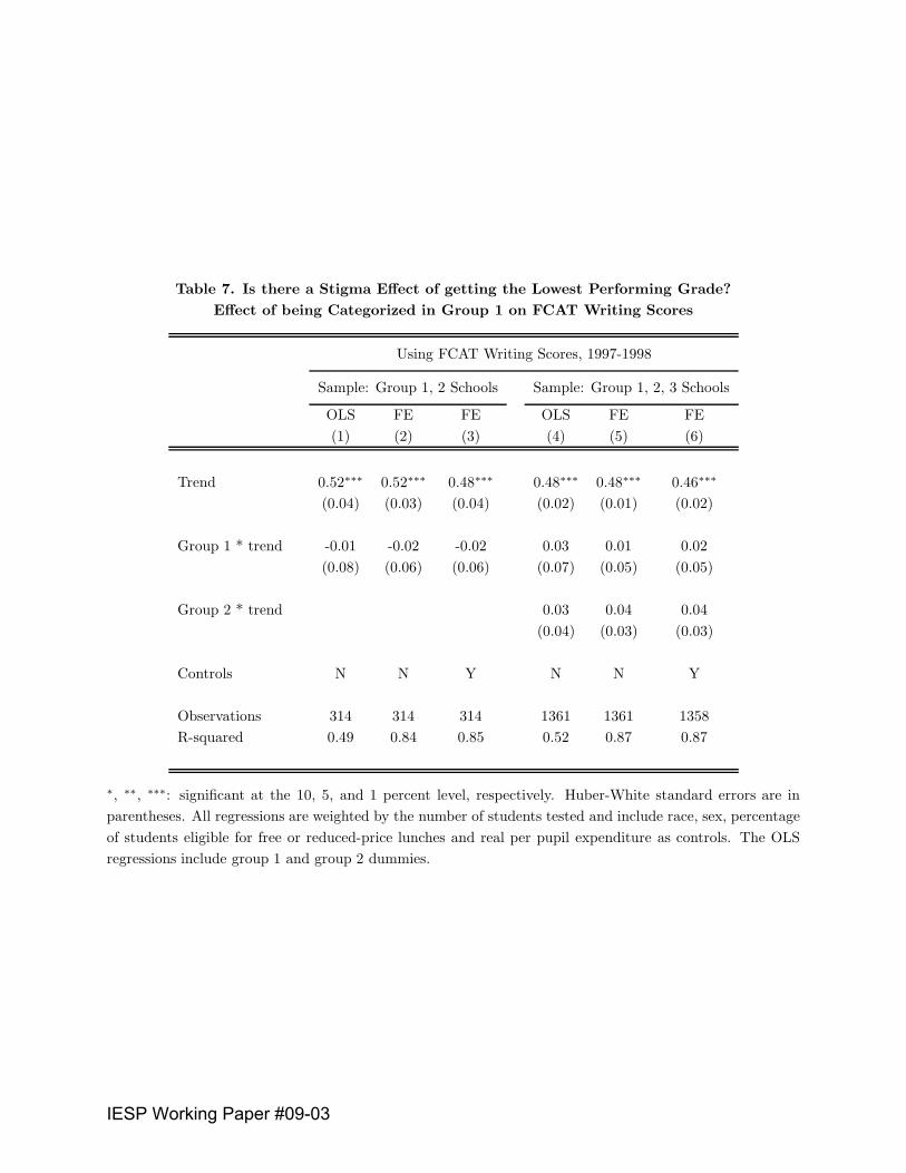
Table 7. Is there a Stigma Effect of getting the Lowest Performing Grade?
Effect of being Categorized in Group 1 on FCAT Writing Scores
Using FCAT Writing Scores, 1997-1998
Sample: Group 1, 2 Schools Sample: Group 1, 2, 3 Schools
OLS FE FE OLS FE FE
(1) (2) (3) (4) (5) (6)
Trend 0.52∗∗∗ 0.52∗∗∗ 0.48∗∗∗ 0.48∗∗∗ 0.48∗∗∗ 0.46∗∗∗
(0.04) (0.03) (0.04) (0.02) (0.01) (0.02)
Group 1 * trend -0.01 -0.02 -0.02 0.03 0.01 0.02
(0.08) (0.06) (0.06) (0.07) (0.05) (0.05)
Group 2 * trend 0.03 0.04 0.04
(0.04) (0.03) (0.03)
Controls N N Y N N Y
Observations 314 314 314 1361 1361 1358
R-squared 0.49 0.84 0.85 0.52 0.87 0.87
∗, ∗∗, ∗∗∗: significant at the 10, 5, and 1 percent level, respectively. Huber-White standard errors are in
parentheses. All regressions are weighted by the number of students tested and include race, sex, percentage
of students eligible for free or reduced-price lunches and real per pupil expenditure as controls. The OLS
regressions include group 1 and group 2 dummies.
IESP Working Paper #09-03

Table 8: Milwaukee Parental Choice Program: Membership
Year Number of Voucher∗ MPS Year Number of Voucher∗ MPS
Schools Students Students Schools Students Students
1990-91 7 300 1997-98 23 1497 101,253
1991-92 6 512 93,381 1998-99 83 5761 99,814
1992-93 11 594 94,258 1999-00 90 7575 99,729
1993-94 12 704 95,258 2000-01 100 9238 97,985
1994-95 12 771 98,009 2000-01 100 9238 97,985
1995-96 17 1288 98,378 2001-02 102 10497 97,762
1996-97 20 1616 101,007 2002-03 102 11350 97,293
∗ “Voucher Students” is calculated as the average of September and January FTE, plus summer school.
Table 9: Comparing the impact of Florida and Milwaukee phase II programs
Using reading [WKCE 1997-2002 and FCAT 1998-2002] and math test [WKCE 1997-2002 and FCAT 1998-2002]
Corrected for Mean Reversion
Reading Math Reading Math
Wisconsin Florida Wisconsin Florida Wisconsin Florida Wisconsin Florida
WKCE FCAT WKCE FCAT WKCE FCAT WKCE FCAT
(1) (2) (3) (4) (5) (6) (7) (8)
More Treated * 1 year 0.20 0.47∗∗∗ 0.27 0.45∗∗∗ 0.20 0.47∗∗∗ 0.03 0.24∗∗∗
More treated * 2 years 0.50∗∗∗ 0.50∗∗∗ 0.38∗∗∗ 0.55∗∗∗ 0.50∗∗∗ 0.50∗∗∗ 0.14∗∗∗ 0.34∗∗∗
More treated * 3 years 0.53∗∗∗ 0.80∗∗∗ 0.57∗∗∗ 0.60∗∗∗ 0.53∗∗∗ 0.80∗∗∗ 0.33∗∗∗ 0.39∗∗∗
All figures are in terms of respective sample standard deviations. All figures are obtained from regressions that contain school
fixed effects, year dummies, interactions of year dummies with the respective treatment dummies, race, sex, free-reduced lunch
percentage and real per pupil expenditure. Standard deviation of FCAT reading scores = 20, Standard deviation of FCAT
Math Scores = 20, Standard deviation of WKCE reading scores = 13.07, Standard deviation of WKCE math scores = 15.01,
Standard Deviation of WKCE Math for the mean reversion sample=14.4, Standard Deviation of FCAT Math for the mean
reversion sample= 20.04
IESP Working Paper #09-03
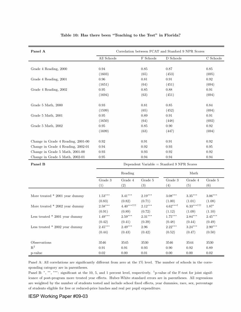
Table 10: Has there been “Teaching to the Test” in Florida?
Panel A Correlation between FCAT and Stanford 9 NPR Scores
All Schools F Schools D Schools C Schools
Grade 4 Reading, 2000 0.94 0.85 0.87 0.85
(1603) (65) (453) (695)
Grade 4 Reading, 2001 0.96 0.81 0.91 0.92
(1651) (64) (451) (694)
Grade 4 Reading, 2002 0.95 0.85 0.88 0.91
(1694) (63) (451) (694)
Grade 5 Math, 2000 0.93 0.81 0.85 0.84
(1599) (65) (452) (694)
Grade 5 Math, 2001 0.95 0.89 0.91 0.91
(1650) (64) (448) (692)
Grade 5 Math, 2002 0.95 0.85 0.90 0.92
(1699) (63) (447) (694)
Change in Grade 4 Reading, 2001-00 0.92 0.91 0.91 0.92
Change in Grade 4 Reading, 2002-01 0.94 0.92 0.93 0.95
Change in Grade 5 Math, 2001-00 0.93 0.93 0.92 0.92
Change in Grade 5 Math, 2002-01 0.95 0.94 0.94 0.94
Panel B Dependent Variable = Stanford 9 NPR Scores
Reading Math
Grade 3 Grade 4 Grade 5 Grade 3 Grade 4 Grade 5
(1) (2) (3) (4) (5) (6)
More treated * 2001 year dummy 1.53∗∗∗ 3.41∗∗∗ 2.19∗∗∗ 3.08∗∗∗ 3.35∗∗∗ 3.06∗∗∗
(0.83) (0.82) (0.71) (1.00) (1.01) (1.08)
More treated * 2002 year dummy 2.58∗∗∗ 4.40∗∗∗††† 2.12∗∗∗ 4.62∗∗∗† 6.33∗∗∗††† 1.87∗
(0.91) (0.89) (0.72) (1.12) (1.09) (1.10)
Less treated * 2001 year dummy 1.49∗∗∗ 2.59∗∗∗ 2.31∗∗∗ 1.75∗∗∗ 2.84∗∗∗ 2.45∗∗∗
(0.42) (0.41) (0.39) (0.48) (0.44) (0.49)
Less treated * 2002 year dummy 2.45∗∗∗ 2.49∗∗∗ 2.96 2.22∗∗∗ 3.24∗∗∗ 2.90∗∗∗
(0.44) (0.43) (0.42) (0.52) (0.47) (0.50)
Observations 3546 3545 3530 3546 3544 3530
R2 0.91 0.91 0.93 0.90 0.92 0.89
p-value 0.02 0.00 0.01 0.00 0.00 0.02
Panel A: All correlations are significantly different from zero at the 1% level. The number of schools in the corre-
sponding category are in parentheses.
Panel B: ∗, ∗∗, ∗∗∗: significant at the 10, 5, and 1 percent level, respectively. 1p-value of the F-test for joint signif-
icance of post-program more treated year effects. Huber-White standard errors are in parentheses. All regressions
are weighted by the number of students tested and include school fixed effects, year dummies, race, sex, percentage
of students eligible for free or reduced-price lunches and real per pupil expenditure.
IESP Working Paper #09-03
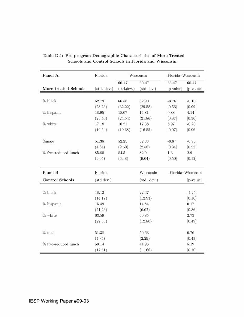
Table D.1: Pre-program Demographic Characteristics of More Treated
Schools and Control Schools in Florida and Wisconsin
Panel A Florida Wisconsin Florida–Wisconsin
66-47 60-47 66-47 60-47
More treated Schools (std. dev.) (std.dev.) (std.dev.) [p-value] [p-value]
% black 62.79 66.55 62.90 -3.76 -0.10
(28.23) (32.22) (29.58) [0.56] [0.99]
% hispanic 18.95 18.07 14.81 0.88 4.14
(23.40) (24.54) (21.86) [0.87] [0.36]
% white 17.18 10.21 17.38 6.97 -0.20
(19.54) (10.68) (16.55) [0.07] [0.96]
%male 51.38 52.25 52.33 -0.87 -0.95
(4.84) (2.60) (2.58) [0.34] [0.22]
% free-reduced lunch 85.80 84.5 82.9 1.3 2.9
(9.95) (6.48) (9.04) [0.50] [0.12]
Panel B Florida Wisconsin Florida–Wisconsin
Control Schools (std.dev.) (std. dev.) [p-value]
% black 18.12 22.37 -4.25
(14.17) (12.93) [0.10]
% hispanic 15.49 14.84 0.17
(21.23) (6.02) [0.86]
% white 63.59 60.85 2.73
(22.33) (12.80) [0.49]
% male 51.38 50.63 0.76
(4.84) (2.29) [0.43]
% free-reduced lunch 50.14 44.95 5.19
(17.51) (11.66) [0.10]
IESP Working Paper #09-03

FCAT Reading, Math and Writing-F,D Schools
Figure 1. Florida 'threat of voucher' Program
FCAT ReadingYEAR
F D
1998 1999 2000 2001 2002
245
255
265
275
285
FCAT MathYEAR
F D
1998 1999 2000 2001 2002
275
285
295
FCAT writingyear
F D
1998 1999 2000 2001 2002
2.4
2.6
2.8
3
3.2
IESP Working Paper #09-03
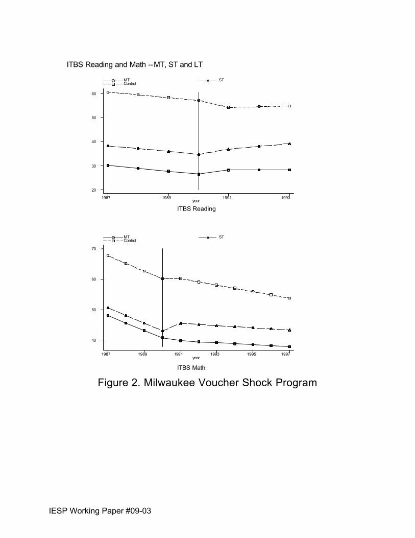
ITBS Reading and Math --MT, ST and LT
Figure 2. Milwaukee Voucher Shock Program
ITBS Reading year
MT ST Control
1987 1989 1991 1993 20
30
40
50
60
ITBS Math year
MT ST Control
1987 1989 1991 1993 1995 1997
40
50
60
70
IESP Working Paper #09-03
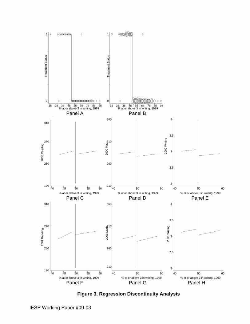
Figure 3. Regression Discontinuity Analysis
Trea
tmen
t Sta
tus
Panel A % at or above 3 in writing, 1999 15 25 35 45 55 65 75 85 95
0
1
Trea
tmen
t Sta
tus
Panel B% at or above 3 in writing, 1999
15 25 35 45 55 65 75 85 95
0
1
2000
Rea
ding
Panel C % at or above 3 in writing, 1999
40 45 50 55 60190
230
270
310
2000
Mat
h
Panel D% at or above 3 in writing, 1999
40 50 60210
260
310
360
2000
Writ
ing
Panel E% at or above 3 in writing, 1999
40 50 60
2
2.5
3
3.5
4
2001
Rea
ding
Panel F % at or above 3 in writing, 1999
40 45 50 55 60190
230
270
310
2001
Mat
h
Panel G% at or above 3 in writing, 1999
40 50 60
210
260
310
360
2001
Writ
ing
Panel H% at or above 3 in writing, 1999
40 50 60
2
2.5
3
3.5
4
IESP Working Paper #09-03

The Institute for Education and Social Policy of the Steinhardt School of Culture, Education, and Human Development and Robert F. Wagner School of Public Service at NYU conducts non-partisan scientific research about U.S. education and related social issues. Our research, policy studies, evalu-ations, seminar series, and technical assistance inform and support policy makers, educators, parents and others in their efforts to improve public schooling. More information is available on our website at http://steinhardt.nyu.edu/iesp.
82 Washington Square East, 7th Floor New York, NY 10003 p 212.998.5880 f 212.995.4564