Research Memorandum 05/2021

27 May 2021

IMPACT OF TREASURY SUPPLY AND THE FED’S ASSET PURCHASES ON

THE US TREASURY YIELD CURVE

Key points

In the US, the rapid vaccine rollout and rounds of fiscal stimulus have

brightened growth prospects, fuelling market expectations of higher future

inflation and earlier Fed tightening. The burgeoning fiscal deficits , which are

unlikely to be fully accommodated by the Fed, have also raised concerns that

markets will have to absorb a much larger supply of Treasuries going forward.

Accordingly, longer-term US Treasury yields have increased sharply since early

2021.

In theory, longer-term Treasury yields are the sum of expected average levels of

short-term real rates and inflation over the bond tenor (collectively known as

the “risk-neutral yields”) and term premia, the last component being the

additional compensation investors require for bearing the risks of holding long-

term Treasuries over short-term ones. While the risk-neutral yields are not likely

to rise strongly further given the Fed’s commitment to keeping short-term rates

low for at least a few more years under its new policy framework, and as

inflation expectations have already picked up notably, the Fed signalled no

intention of adjusting its quantitative easing (QE) programme to counter upward

pressures on longer-term yields, implying that term premia are likely to be the

main driving force of longer-term yields going forward.

Generally speaking, term premia are influenced by factors such as the demand-

supply balance of Treasury securities (which in turn depends on the Fed’s QE)

and the uncertainty over future yields. This paper studies the Treasury term

premia for maturities up to ten years, examining how they could be affected by

the net Treasury supply (i.e. gross issuance net of Fed purchases) after

2

controlling for other market and macroeconomic conditions. Our estimation

results allow us to construct yield curves under different scenarios of the Fed’s

QE policy, taking as given the prevailing expected future paths of real short-

term rates and inflation.

Based on projections of new Treasury issuance from the US Department of the

Treasury’s latest Quarterly Refunding Statement , our baseline results point to a

10-year yield at 2.1% by the end of 2021. If, assuming that the Fed is able to

communicate its policy intentions clearly and convince markets that a QE

tapering is not a harbinger of imminent rate hikes, a tapering of QE purchases

that begins in Q4 2021 can be expected to drive up the 10-year yield modestly,

by additional 6-13 basis points (bps) relative to the baseline.

However, in an adverse scenario where the Fed mis-communicates its tapering

decision and triggers a “taper tantrum” type of reactions from the market like

in 2013, our estimate suggests that the 10-year yield may surge to 2.8%, a jump

of 73 bps above the baseline case.

It should be emphasised that this study is a scenario analysis, rather than an

attempt to forecast future Treasury yields. Indeed, the future trajectory of US

Treasury yields can be affected by many factors that are subject to considerable

uncertainties, such as the government’s future financing needs and the

vicissitudes of market risk appetite.

Prepared by: Shifu Jiang and Eric Tsang*

Economic Research Division, Research Department

Hong Kong Monetary Authority

* The authors would like to thank Lillian Cheung, Michael Cheng and Ka-Fai Li for their helpful comments

and suggestions.

The views and analysis expressed in this paper are those of the authors, and do not

necessarily represent the views of the Hong Kong Monetary Authority.

3

I. INTRODUCTION

The ascent of longer-term US Treasury yields accelerated sharply since

early 2021, partially due to the rapid vaccine rollout and a new round of fiscal

stimulus in the form of a US$1.9 trillion American Rescue Plan, which have

brightened growth prospects and fuelled market expectations of higher inflation and

earlier Fed tightening (via tapering QE and/or hiking policy rates). The pickup in

yields also reflects market concerns that the burgeoning fiscal deficits may

necessitate much higher Treasury issuance down the road, especially if the rest of

President Biden’s “Build Back Better” agenda (including the “American Jobs Plan”

and the “American Families Plan” with headline price tags of over US$2 trillion and

US$1.8 trillion respectively) is enacted but higher corporate taxes are insufficient to

cover the expenditure.

2. To better understand the drivers behind the recent rise in longer-term

Treasury yields, it is useful to decompose them as the sum of expected average levels

of short-term real rates and inflation over the bond tenor (collectively known as “risk-

neutral yields”) and term premia. The last component arises because risk-averse

investors have preferences for specific maturities, and if they are going to hold long-

term bonds instead of short-term ones, they require additional compensation for

adjusting their portfolios and bearing the risks that the actual path of risk-neutral

yields may deviate from expectations. Term premia, in turn, are influenced by a

multitude of factors such as the demand-supply balance of Treasury securities and

uncertainties over the future path of yields and inflation.

3. Chart 1 shows the decomposition of 10-year nominal US Treasury

yield (grey line) into the risk-neutral yield (red line) and the term premium (blue line).

It can be seen from the chart that a significant part of the rise in 10-year yield since

early 2021 can be attributed to rising term premium, which forms the key motivation

behind this study.

4

Chart 1: 10-year nominal US

Treasury yield decomposition

Note: Data shown in this chart refer to the 10Y

zero-coupon (i.e. spot) Treasury yield. Term

premium is estimated by Wu and Xia (2016)’s

approach.

Source: HKMA staff calculations.

4. An increase in the risk-neutral and term premium components of

longer-term yields can have different market and macroeconomic implications. On

one hand, a higher risk-neutral rate reflecting better growth expectation does not

necessarily tighten financial conditions. On the other hand, higher US term premia

could lead to a premature tightening of global financial conditions via spillovers to

other sovereign debt markets1 . As pointed out by IMF’s latest Global Financial

Stability Report (April 2021, Chapter 1), a sharp rise in US term premia could lead

to an unfavourable snapback in local currency term premia in emerging markets, with

a 1 percentage point increase in the former estimated to drive up the latter by 60 basis

points on average.

5. The relative importance of the risk-neutral versus term premia

components in driving future longer-term yields also depends on monetary policy

settings. The former is unlikely to move much higher in the near future given the

Fed’s strong commitment to keeping short-term rates low for at least a few more

years, as well as the already-sizeable uptick in inflation expectations since early 2021.

However, the Fed has signalled no intention of adjusting its QE programme to

counter upward pressures on longer-term yields, leaving room for greater

decompression of term premia. For example, upside risks to term premia could

emerge if a larger-than-expected portion of fiscal spending is financed by longer-

term government debt, or if larger-than-expected further progress towards full

1 See, for example, “Term Premium Spillovers from the US to International Markets”, HKMA Research

Memorandum 2017/05.

5

employment prompts the Fed to start tapering asset purchases.

6. These considerations lead us to conduct an empirical study of term

premia, focusing particularly on its relationship with net Treasury supply (i.e. total

outstanding Treasuries minus Fed holdings). The rest of the paper is organised as

follows. Section II lays out the empirical framework and discusses data. Section III

elaborates on the estimation results and examines scenarios of Treasury yield risks.

Section IV provides policy implications and concludes.

II. EMPIRICAL FRAMEWORK AND DATA

7. In this study, we regress nominal US Treasury term premia for

tenors up to 10 years, which are estimated by Wu and Xia (2016)’s method2,

on a measure of net Treasury supply and other control variables over the

monthly sample period from July 2003 to December 2020, during which data

is available3.

8. To construct a measure of Treasury supply, we follow Greenwood and

Vayanos (2014) and use maturity-weighted debt (MWD) to capture the duration

risk that investors must bear. MWD is the sum of cash flows (including coupons and

the principal) weighted by their maturity across individual bonds that are active in

each period. To this end, we collect data on every US Treasury bill, bond, and note

from the Department of the Treasury's Monthly Statement of the Public Debt and the

New York Fed's System Open Market Account. Let 𝑀𝑊𝐷𝑡 denote the total

outstanding maturity-weighted Treasury debt net of inter-agency holdings,

𝑀𝑊𝐷𝑡𝐹𝑒𝑑 the amount held by the Fed, then the net Treasury supply is given by

𝑀𝑊𝐷𝑡 −𝑀𝑊𝐷𝑡𝐹𝑒𝑑, which is scaled by trend GDP throughout the rest of the paper.

Chart 2 shows that the net Treasury supply dropped shortly after the announcements

of QE1, QE2 and the most recent restart of QE following the COVID-19 pandemic,

2 Wu and Xia (2016)’s method of estimating term premia allows us to take into account the effective lower

bound, which binds in a considerable proportion of our sample period. Nonetheless, the dynamics of our

estimates are similar to those of Kim and Wright (2005) and other well-known estimates (e.g. Cohen, Hördahl

and Xia 2018) that do not correct for the effective lower bound. On a separate matter, Bauer, Rudebusch, and

Wu (2014) note that estimates of term premia could suffer from small-sample bias such that term premia

explain too much of the yield variances. While their bias-correction bootstrapping procedure cannot be directly

applied when the underlying factors are unobservable as in our case, our 375-observation monthly sample (Jan

1990 – April 2021) should suffer from a much smaller bias comparing to the 77-observation quarterly sample

(Q1 1990 – Q1 2009) considered in their study. 3 It is important to use term premia instead of Treasury yields in the empirical model because the latter are

significantly affected the Fed’s forward guidance, which is difficult to model.

6

while showing an uptrend sometime after the announcement of QE tapering in end-

2013.4

Chart 2: Measure of net Treasury

supply

Chart 3: Correlation between the 10-

year term premium and net Treasury

supply

Source: HKMA staff calculations.

Source: HKMA staff calculations.

Note: In this chart, QE1 refers to purchases of US Treasuries under the Fed’s large scale asset purchase

programme 1, which was announced in March 2009, later than MBS purchases.

9. Net Treasury supply affects term premia through a portfolio

balance channel, which has received great attention because it is one of the

primary transmission channels of QE. Consider an increase in the supply of

longer-term Treasury either due to the government’s financing need or the

Fed’s tapering of QE. A clientele of long-horizon investors (e.g. pension

funds and insurance companies) would be willing to absorb those bonds , and

hence bear more risk, only if they were compensated by an increase in long-

term yields relative to short-term yields. This effect is expected to be stronger

on longer-term yields because of greater duration risk. Meanwhile, short rates,

determined mainly by conventional monetary policy and short-horizon

investors (e.g. money-market mutual funds), might not be affected

significantly.

10. To estimate the effect of a Treasury supply shock on term premia, it is

necessary to identify movements in the supply that are exogenous to those of term

premia. Before the Global Financial Crisis, US Treasury supply was largely

exogenous, in the sense that changes in Treasury supply affected term premia, but

4 Net Treasury supply has started its downward trend by the end of 2011, well before QE3, because

government deficit began to narrow at that time.

7

not the other way around. However, the implementation of QE means that the Fed

adjusts net Treasury supply endogenously in response to changes in term premia,

posing a challenge to the estimation using a sample when QE was active. Indeed,

Chart 3 shows a positive correlation between the term premium and net supply before

QE as expected, but a negative correlation thereafter. To overcome this issue, we

follow the identification strategy of a public spending shock in the fiscal multiplier

literature and employ military expenditure (again scaled by trend GDP) as an

instrumental variable for net Treasury supply. The idea is that US military

expenditure is driven by global geopolitical factors and not domestic economic

conditions. Moreover, US wars in recent history have been fought primarily on

foreign soil and have had no impact on macroeconomic outcomes except through the

increases in public spending they induced. Finally, military expenditure is arguably

financed more by debt than by taxes, making it a relevant instrument.

11. Our empirical model also contains the following control variables that

are popular in the literature (e.g. d’Amico et al. 2012, Gagnon et al. 2010).5

One month lagged yield curve slope: Measured by the spread between the 2-year

yield and the yield over the maturity under consideration. If the dependent

variable is the 2-year term premium, the spread between the 1- and 2-year yields

is used. The slope variable has been widely found to be a predictor of both

economic activity and Treasury returns, and is expected to have a positive

correlation with term premia.

Unemployment gap: Measured as the difference between the unemployment rate

and the Congressional Budget Office’s estimate of the natural rate of

unemployment. This variable is useful to capture the prevailing stage of business

cycles. This variable may be positively or negatively correlated with term

premia, depending on the nature of the underlying driving forces of business

cycles.

MOVE index: A proxy for short-term interest rate uncertainty. In practice, we

find the MOVE index has significant and positive explanatory power only

during market turmoil such as the immediate aftermath of the global financial

crisis (roughly the QE1 period), and in the second quarter of 2020 when the

economic damage of the COVID-19 lockdown measures was felt most strongly.

5 Other control variables that turn out to be insignificant include past inflation and VIX. We also do not include

variables capturing QE news because QE announcements are followed closed by actions, typically within the

same month.

8

During these periods, QE was deployed as an emergency response to financial

market dislocations and could be conducted in a qualitatively different manner

than other periods. Moreover, during those volatile periods the Fed was

essentially the only dominant buyer in the Treasury market, meaning that the

concept of “demand for Treasuries” was inapplicable. The MOVE index is

multiplied by dummy variables representing such periods.

Long-term inflation uncertainty: Measured by the difference between 75% and

25% quantiles of 10-year CPI inflation expectations, collected from the

Philadelphia Fed’s Survey of Professional Forecasters. This variable captures

the dispersion among inflation expectations and serves as a proxy of uncertainty

about long-term inflation.6 It is expected to have a positive correlation with term

premia, as investors facing larger inflation uncertainty will likely demand for a

larger term premium as compensation for holding long-term bonds.

III. ESTIMATION RESULTS AND SCENARIO ANALYSIS

12. Since the Treasury market has likely experienced a major structural

break during the global financial crisis, we run the regressions using two sub-samples.

In the pre-QE sample (July 2003 – March 2009), the model is estimated by ordinary

least squares. In the post-QE sample (March 2009 – Dec 2020), the model is

estimated by two-stage least square approach using military spending as an

instrumental variable to control for movements of net Treasury supply that were

endogenous to Treasury yields. The estimation results for each of the 2-, 5-, 7-, and

10-year term premium are reported in Table 1.

6 Wright (2011), for example, offered cross-country empirical evidence that term premia tended to decline

along with reduced inflation uncertainty.

9

Table 1: Results from term premium regression

Tenor Net

Treasury

supply

Yield

curve slope

Unemp.

gap MOVE

Inflation

uncertainty

Adjusted

R2

Pre-QE

2 0.20 0.74*** -0.11*** 0.001** 0.22** 0.84

5 0.45** 0.53*** -0.17*** 0.000 0.24* 0.79

7 0.67** 0.34*** -0.20*** 0.002 0.37** 0.75

10 0.87** 0.26*** -0.21*** 0.003* 0.47** 0.75

Post-QE

2 0.50** 1.22*** -0.18** 0.003*** 0.39** 0.78

5 1.48*** 1.22*** -0.09*** 0.010** 0.84** 0.76

7 1.82** 1.07*** -0.12*** 0.014** 0.97** 0.77

10 2.15*** 1.01*** -0.14*** 0.017** 1.06** 0.79

Note: *, ** and *** denote statistical significance at 10%, 5% and 1% level respectively.

Sources: HKMA staff calculations.

13. Table 1 shows that net Treasury supply (column shaded in light grey)

has a statistically significant and positive impact on longer-term premia in both sub-

samples. However, the quantitative effect is considerably stronger in the post-GFC

sample, ranging from 50 to 215 bps, comparing to 20 to 87 bps in the pre-GFC

sample. Across the yield curve, the supply effect is smaller the shorter the maturity

becomes and can be insignificant on the 2-year term premium, which is as expected

because data clearly shows that shorter-term yields are better anchored by the Fed.

This means that a net Treasury supply shock tends to make the yield curve steeper,

especially in the post-QE sample. Finally, we note that term premia have become

more responsive to risks and market conditions (i.e. Treasury supply, yield curve

slope, inflation uncertainties and MOVE) than to the stage of business cycle (i.e.

unemployment gap) in the post-QE sample period.

Scenario settings

14. To put the estimation results in context, we construct four scenarios for

the end of 2021, with the scenarios differing in the pace of Fed’s QE and the presence

of a taper tantrum effect, to examine how net Treasury supply affects the yield curve.

Specifically, our baseline case assumes that the Fed maintains its current pace of asset

purchases. Meanwhile in the first two Scenarios, we assume that the Fed can

perfectly communicate its policy intentions and, aided by the new “inflation makeup”

10

monetary policy framework, convince investors that QE tapering and rate hikes are

two separate issues, such that a reduction or a stop in the Fed’s asset purchases do

not pull forward markets’ rate hike expectations. Finally, in the “Taper Tantrum

Redux” Scenario, we instead assume that the Fed mis-communicates its tapering

decision, and triggers a repeat of the 2013 “Taper Tantrum” episode.

The detailed assumptions of each Scenario are as follows:

Baseline scenario: In this scenario, net Treasury supply at the end of 2021 is

calculated assuming that new issuances of Treasury securities in Q4 2021 follow

the same pattern as that outlined in the Q3 2021 “TBAC (Treasury Borrowing

Advisory Committee) Recommended Financing Table”, contained in the latest

set of Quarterly Refunding Documents published by the US Department of the

Treasury on 5 May 2021.7 Meanwhile, the Fed’s Treasury holdings at the end of

2021 are calculated assuming that QE remains at the same pace as of 5 May 2021,

to be consistent with the assumption about Treasury issuance as outlined in the

Quarterly Refunding Statement issued on the same day. Together, these

assumptions imply that net Treasury supply will rise to 2.75 by end-2021 (please

see chart 2 for a visualisation of this measure of Treasury supply) from 2.60 in

April 2021.

Scenario 1 (“Half-tapering”): With everything else remaining the same, the pace

of QE is halved in Q4 2021 relative to the baseline scenario, increasing net

Treasury supply to 2.78. Meanwhile, markets’ expectations of the future policy

rate path are assumed to remain unchanged, thanks to clear communications by

the Fed that convinces markets that the “low-for-long” forward guidance would

remain intact even after QE tapering begins.

Scenario 2 (“Full-tapering”): Everything else remains the same as in the baseline

scenario, except that QE is assumed to halt completely in Q4 2021, thereby

increasing net Treasury supply to 2.81. Again, this scenario assumes that markets’

expectations of the future path of short rates remain unchanged.

7 Since each set of Quarterly Refunding Documents only provides projections of Treasury issuance for the

current quarter and the next (i.e. the latest version covering Q2 and Q3 2021), we have to make an additional

assumption that the Q4 issuance of Treasuries follows the same pattern as in Q3, in order to allow us to examine

scenarios for end-2021. Such an assumption can be justified by the Treasury Department’s latest Quarterly

Refunding Statement that it believes the current issuance sizes, which have been substantially increased

compared to a year ago, should be sufficient to cover near-term projected borrowing needs, hence no imminent

need to change the auction sizes of longer-term Treasuries again. Indeed, the Q3 TBAC financing table is

almost identical to the one for Q2, and we therefore expect a similar pattern for Q4 as well.

11

Scenario 3 (“Taper Tantrum Redux”): On top of the “full-tapering” scenario, we

assume the Fed mis-communicates its policy intention, thereby triggering a full-

blown “taper tantrum” type of reactions from the market. The taper tantrum effect

is estimated as the sum of three factors: (1) the movements in the risk-neutral

interest rates between May and September 2013 to capture shifts in expectations

about future federal funds rates, (2) the model-implied contribution of the MOVE

index to term premia during the same period to capture market panic, and (3) the

difference between the actual and model-implied term premia in May 2013 to

capture the effect beyond market and macroeconomic conditions.

All control variables remain at their current levels unless otherwise stated.

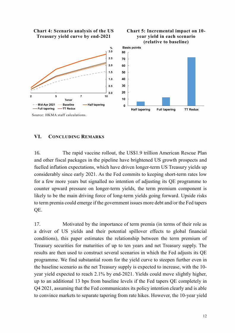
15. Chart 4 shows the yield curves constructed in each scenario (as well as

the actual one as of mid-April, in dotted grey line, for ease of comparison), and Chart

5 shows the incremental changes in 10-year yield (relative to baseline) as one moves

from Scenario 1 to Scenario 3. Our baseline scenario suggests substantial room for

the yield curve to drift upward and steepen from the current level, with the 10-year

yield reaching 2.08% by the end of 2021. In the two tapering scenarios, if the market

does not pull forward rate hike expectations and remains calm (i.e. in the absence of

“taper tantrum” type of shocks), the supply factor alone implies some additional,

modest steepening of the yield curve compared to the baseline. Specifically, the 10-

year yield is projected to increase to 2.16% and 2.21% under the “half tapering” and

“full tapering” scenarios respectively. However, if a “taper tantrum” type of market

shock is triggered as in the “Redux” scenario, the 10-year yield could possibly surge

to as high as 2.81%, a 73 bps increase over the baseline case.

12

Chart 4: Scenario analysis of the US

Treasury yield curve by end-2021

Chart 5: Incremental impact on 10-

year yield in each scenario

(relative to baseline)

Source: HKMA staff calculations.

VI. CONCLUDING REMARKS

16. The rapid vaccine rollout, the US$1.9 trillion American Rescue Plan

and other fiscal packages in the pipeline have brightened US growth prospects and

fuelled inflation expectations, which have driven longer-term US Treasury yields up

considerably since early 2021. As the Fed commits to keeping short-term rates low

for a few more years but signalled no intention of adjusting its QE programme to

counter upward pressure on longer-term yields, the term premium component is

likely to be the main driving force of long-term yields going forward. Upside risks

to term premia could emerge if the government issues more debt and/or the Fed tapers

QE.

17. Motivated by the importance of term premia (in terms of their role as

a driver of US yields and their potential spillover effects to global financial

conditions), this paper estimates the relationship between the term premium of

Treasury securities for maturities of up to ten years and net Treasury supply. The

results are then used to construct several scenarios in which the Fed adjusts its QE

programme. We find substantial room for the yield curve to steepen further even in

the baseline scenario as the net Treasury supply is expected to increase, with the 10-

year yield expected to reach 2.1% by end-2021. Yields could move slightly higher,

up to an additional 13 bps from baseline levels if the Fed tapers QE completely in

Q4 2021, assuming that the Fed communicates its policy intention clearly and is able

to convince markets to separate tapering from rate hikes. However, the 10-year yield

13

may surge by 73 bps relative to the baseline if the Fed’s communication triggers

a “taper tantrum” type of reactions from the market. This study highlights the

risks of a premature tightening of global financial conditions and financial market

volatility if net Treasury supply increases further, and the importance of clear central

bank communication in order to avoid inadvertently triggering another round of

“taper tantrum”.

18. Care should be taken when interpreting the estimated Treasury yields.

It should be emphasised that this study serves as a scenario analysis, rather than

providing forecasts of future US Treasury yields. Indeed, the future trajectory of

US Treasury yields can be affected by many factors that are subject to

considerable uncertainties, such as the government’s future financing needs

and the vicissitudes of market risk appetite.

14

REFERENCES

Bauer, M.D., Rudebusch, G.D. and Wu, J.C., 2014. Term premia and inflation

uncertainty: Empirical evidence from an international panel dataset: Comment.

American Economic Review, 104(1), pp.323-37.

Cohen, B.H., Hördahl, P. and Xia, F.D., 2018. Term premia: models and some

stylised facts. BIS Quarterly Review September.

d’Amico, S., English, W., López‐Salido, D. and Nelson, E., 2012. The Federal

Reserve's large‐scale asset purchase programmes: rationale and effects. The

Economic Journal, 122(564), pp.F415-F446.

Gagnon, J., Raskin, M., Remache, J. and Sack, B.P., 2010. Large-scale asset

purchases by the Federal Reserve: did they work?. FRB of New York Staff Report,

(441).

Greenwood, R. and Vayanos, D., 2014. Bond supply and excess bond returns. The

Review of Financial Studies, 27(3), pp.663-713.

Kim, D.H. and Wright, J.H., 2005. An arbitrage-free three-factor term structure

model and the recent behavior of long-term yields and distant-horizon forward rates.

Li, K.F., Fong, T. and Ho, E., 2017. Term Premium Spillovers from the US to

International Markets. HKMA Research Memorandum, 05.

Wright, J., 2011. Term premia and inflation uncertainty: Empirical evidence from an

international panel dataset. The American Economic Review, 101(4), 1514-1534.

Wu, J.C. and Xia, F.D., 2016. Measuring the macroeconomic impact of monetary

policy at the zero lower bound. Journal of Money, Credit and Banking, 48(2-3),

pp.253-291.