Impact of regularization on Spectral Clustering

Antony Joseph∗and Bin Yu†

December 5, 2013

Abstract

The performance of spectral clustering is considerably improved viaregularization, as demonstrated empirically in Amini et al. [2]. Here, weprovide an attempt at quantifying this improvement through theoreticalanalysis. Under the stochastic block model (SBM), and its extensions,previous results on spectral clustering relied on the minimum degree ofthe graph being sufficiently large for its good performance. We prove thatfor an appropriate choice of regularization parameter τ , cluster recoveryresults can be obtained even in scenarios where the minimum degree issmall. More importantly, we show the usefulness of regularization in situ-ations where not all nodes belong to well-defined clusters. Our results relyon the analysis of the spectrum of the Laplacian as a function of τ . Asa byproduct of our bounds, we propose a data-driven technique DK-est(standing for estimated Davis-Kahn bounds), for choosing the regulariza-tion parameter. This technique is shown to work well through simulationsand on a real data set.

1 Introduction

The problem of identifying communities, or clusters, in large networks is animportant contemporary problem in statistics. Spectral clustering is one of themore popular techniques for such purposes, chiefly due to its computationaladvantage and generality of application. The algorithm’s generality arises fromthe fact that it is not tied to any modeling assumptions on the data, but isrooted in intuitive measures of community structure such as sparsest cut basedmeasures [12], [26], [18], [22]. Other examples of applications of spectral clus-tering include manifold learning [4], image segmentation [26], and text mining[10].

The canonical nature of spectral clustering also generates interest in vari-ants of the technique. Here, we attempt to better understand the impact ofregularized forms of spectral clustering for community detection in networks.

∗Department of Genome Dynamics, Lawrence Berkeley National Laboratory, and Depart-ment of Statistics, University of California, Berkeley. email: AntonyJoseph@lbl.gov†Department of Statistics and EECS, University of California, Berkeley. email:

binyu@stat.berkeley.edu

1

In particular, we focus on the Perturbed Spectral Clustering (PSC) procedureproposed in Amini et al. [2]. Their empirical findings demonstrates that theperformance of the PSC algorithm, in terms of obtaining the correct clusters,is significantly better for certain values of the regularization parameter. Analternative form of regularization was studied in Dasgupta et al. [9], Chaudhuriet al. [7], and Qin and Rohe [24].

This paper provides an attempt to provide a theoretical understanding forthe regularization in the PSC algorithm under the stochastic block model (SBM)framework. We also address the practical issue of the choice of regularizationparameter. The following are the main contributions of the paper.

(a) In Section 3 we demonstrate improvements in eigenvector perturbationbounds through regularization. In particular, for a graph with n nodes,previous theoretical analyses for spectral clustering, under the SBM and itsextensions, [25],[7], [27], [11] assumed that the minimum degree of the graphscales at least by a polynomial power of log n. Even when this assumption issatisfied, the dependence on the minimum degree is highly restrictive whenit comes to making inferences about cluster recovery. Our analysis providesbounds on the perturbation of eigenvectors of the regularized Laplacian.These bounds, when optimized over the regularization parameter, poten-tially do not depend on the above mentioned constraint on the minimumdegree. As an example, for an SBM with two blocks (clusters), our boundsare inversely related to the maximum degree, as opposed to the minimumdegree.

(b) In Section 4 we demonstrate that regularization has the potential of address-ing a situation, often encountered in practice, where not all nodes belongto well-defined clusters. Without regularization, these nodes would hamperwith the clustering of the remaining nodes in the following way: In order forspectral clustering to work, the top eigenvectors - that is, the eigenvectorscorresponding to the largest eigenvalues of the Laplacian - need to be ableto discriminate between the clusters. Due to the effect of nodes that do notbelong to well-defined clusters, these top eigenvectors do not necessarilydiscriminate between the clusters with ordinary spectral clustering. With aproper choice of regularization parameter, we show that this problem canbe rectified. We also demonstrate this on simulated and real datasets.

(c) In Section 6 we provide a data dependent technique for choosing the regu-larization parameter based on our bounds. We demonstrate that it workswell through simulations and on a real data set.

A crucial ingredient in (a) and (b) is the analysis of the spectrum of theLaplacian as a function of the regularization parameter. Assuming that there areK clusters, an adequate gap between the top K eigenvalues and the remainingeigenvalues, ensures that these clusters can be estimated well [28], [22], [18].Such a gap is commonly referred to as the eigen gap. In the situation consideredin (b), an adequate eigen gap may not exist for the unregularized Laplacian.

2

We show that regularization works by creating a gap, allowing us to recover theclusters.

The paper is divided as follows. In the next section we discuss preliminaries.In particular, in Subsection 2.1 we review the PSC algorithm of [2], while inSubsection 2.2 we review the stochastic block model. Our theoretical results,described in (a) and (b) above, are provided in Sections 3 and 4. Section 5discusses the regularization studied in the papers [9], [7], [24] in relation to ourwork. Section 6 describes a data dependent method for choosing the regular-ization parameter, motivated by our bounds. Section 7 provides the high-levelidea behind the proofs of results in Sections 3 and 4.

2 Preliminaries

In this section we review the perturbed spectral clustering (PSC) algorithm ofAmini et al. [2] and the stochastic block model framework.

We first introduce some basic notation. A graph with n nodes and edge setE is represented by the n× n symmetric adjacency matrix A = ((Aij)), whereAij = 1 if there is an edge between i and j, otherwise Aij is 0. In other words,

Aij =

{1, if (i, j) ∈ E0, otherwise

.

Given such a graph, the typical community detection problem is synonymouswith finding a partition of the nodes. A good partitioning would be one in whichthere are few edges between the various components of the partition, comparedto the number of edges within the components. Various measures for goodnessof a partition have been proposed, chiefly the Ratio Cut [12] and NormalizedCut [26] . However, minimization of the above measures is an NP-hard problemsince it involves searching over all partitions of the nodes. The significanceof spectral clustering partly arises from the fact that it provides a continuousapproximation to the above discrete optimization problem [12], [26].

2.1 The PSC Algorithm [2]

We now describe the PSC algorithm [2], which is a regularized version of spec-

tral clustering. Denote by D = diag(d1, . . . , dn) the diagonal matrix of degrees,

where di =∑nj=1Aij . The normalized (unregularized) symmetric graph Lapla-

cian is defined asL = D−1/2AD−1/2.

Regularization is introduced in the following way: Let J be a constant ma-trix with all entries equal to 1/n. Then, in perturbed spectral clustering oneconstructs a new adjacency matrix by adding τJ to the adjacency matrix A andcomputing the corresponding Laplacian. In particular, let

Aτ = A+ τJ,

3

where τ > 0 is the regularization parameter. The corresponding regularizedsymmetric Laplacian is defined as

Lτ = D−1/2τ AτD

−1/2τ .

Here, Dτ = diag(d1,τ , . . . , dn,τ ) is the diagonal matrix of ‘degrees’ of the mod-

ified adjacency matrix Aτ . In other words, di,τ = di + τ .The PSC algorithm for finding K communities is described in Algorithm 1.

The algorithm first computes Vτ , the n×K eigenvector matrix corresponding tothe K largest (in absolute terms) eigenvalues of Lτ . The columns of Vτ are takento be orthogonal. The rows of Vτ , denoted by Vi,τ , for i = 1, . . . , n, correspondsto the nodes in the graph. Clustering the rows of Vτ provides a clustering ofthe nodes. We remark that with τ = 0, the PSC Algorithm 1 corresponds tothe usual spectral clustering algorithm.

We also remark that there is flexibility in the choice of the clustering proce-dure in Step 2 of the algorithm we describe below. A natural choice would bethe k-means algorithm [22], [25], [17]. This was also used for the PSC algorithm[2]. Algorithm 2, proposed in McSherry [20], provides an alternative procedurethat has been used in the literature. This algorithm, along with variants [7], [3],uses pairwise distances of the rows of the eigenvector matrix to do clustering.

Algorithm 1 The PSC algorithm [2] with regularization parameter τ

Input : Laplacian matrix Lτ .Step 1: Compute the n×K eigenvector matrix Vτ .Step 2: Use Algorithm 2 to cluster the rows of Vτ into K clusters.

Our main theoretical results concerns the impact of regularization on per-turbation of eigenvectors. In order to translate these results into implicationsfor cluster recovery, we use Algorithm 2 in Step 2 of the PSC Algorithm 1 sinceit is easier to analyze. Our simulation results will use the k-means algorithm inStep 2 instead.

Algorithm 2 Clustering procedure in McSherry [20] with parameter t > 0.

Input : Data points Vi,τ , for i = 1, . . . , n.

Set k(1) = 1 and S = {2, . . . , n}.while S 6= ∅ do

Choose a j in S at random. Set S = S − {j}.if For some i ∈ Sc, ‖Vj,τ − Vi,τ‖ < t then assign k(j) = k(i).else

If there are unused labels in {1, . . . ,K} then assign a new label

at random for k(j). Otherwise set k(j) = 0.end if

end whileOutput: Function k that provides the cluster labels.

4

In Algorithm 2 we denote by k : {1, . . . , n} → {0, 1, . . . ,K} as the function

that provides cluster labels for the n nodes. The algorithm returns k(i) = 0 ifnode i could not be assigned to any of the K clusters, although in our analysisof clustering performance we show that all nodes are clustered accurately. Theappropriate choice of the parameter t, used as input to the algorithm, will bespecified in Lemma 2.

Our theoretical results assume that the data is randomly generated from astochastic block model (SBM), which we review in the next subsection. While itis well known that there are real data examples where the SBM fails to providea good approximation, we believe that the above provides a good playground forunderstanding the role of regularization in the PSC algorithm. Recent works [2],[11], [25], [6], [16] have used this model, and its variants, to provide a theoreticalanalyses for various community detection algorithms.

Notation

We use ‖.‖ to denote the spectral norm of a matrix. Notice that for vectorsthis corresponds to the usual `2-norm. We use A′ to denote the transpose of amatrix, or vector, A.

For positive an, bn, we use the notation an � bn if there exists universalconstants c1, c2 > 0 so that c1an ≤ bn ≤ c2an. Further, we use bn . an ifbn ≤ c2an, for some c2 not depending on n. The notation bn & an is analogouslydefined.

2.2 The Stochastic Block Model

Given a set of n nodes, the stochastic block model (SBM), introduced in [14],is one among many random graph models that has communities inherent in itsdefinition. We denote the number of communities in the SBM by K. Through-out this paper we assume that K is known. The communities, which representa partition of the n nodes, are assumed to be fixed beforehand. Denote theseby C1, . . . , CK .

Given the communities, the edges between nodes, say i and j, are chosenindependently with probability depending the communities i and j belong to.In particular, for a node i belonging to cluster Ck1 , and node j belonging tocluster Ck2 , the probability of edge between i and j is given by

Pij = Bk1,k2 . (1)

Here, the block probability matrix

B = ((Bk1,k2)), where k1, k2 = 1, . . . ,K

is a symmetric full rank matrix, with each entry between [0, 1].The n × n matrix P = ((Pij)), given by (1), represents the population

counterpart of the adjacency matrix A. From (1), it is seen that the rankof P is also K. This is most readily seen if the nodes are ordered according

5

to the clusters they belong to, in which case P has a block structure with Kblocks. The population counterpart for the degree matrix D is denoted byD = diag(d1, . . . , dn), where D = diag(P1). Here 1 denotes the column vectorof all ones.

Similarly, the population version of the symmetric Laplacian Lτ is denotedby Lτ , where

Lτ = D−1/2τ PτD

−1/2τ .

Here Dτ = D + τI and Pτ = P + τJ. The n× n matrices Dτ and Pτ representthe population counterparts to Dτ and Aτ respectively. Notice that since P hasrank K, the same holds for Lτ .

2.2.1 The Population Cluster Centers

We now proceed to define population cluster centers centk,τ ∈ RK , for k =1, . . . ,K, for the K block SBM. These points are defined so that the rows of theeigenvector matrix Vi,τ , for i ∈ Ck, are expected to be scattered around centk,τ .

Denote by Vτ an n×K matrix containing the eigenvectors of the K largesteigenvalues (in absolute terms) of Lτ . As with Vτ , the columns of Vτ are alsoassumed to be orthogonal.

Notice that both Vτ and −Vτ are eigenvector matrices corresponding to Lτ .This ambiguity in the definition of Vτ is further complicated if an eigenvalue ofLτ has multiplicity greater than one. We do away with this ambiguity in thefollowing way: Let H denote the set of all n × K eigenvector matrices of Lτ

corresponding to the top K eigenvalues. We take,

Vτ = arg minH∈H

‖Vτ −H‖, (2)

The matrix Vτ , as defined above, represents the population counterpart ofthe matrix Vτ .

Let Vi,τ denote the i-th row of Vτ . Notice that since the setH is closed underthe ‖.‖ norm, one has that Vτ is also an eigenvector matrix of Lτ correspondingto the top K eigenvalues. Consequently, the rows Vi,τ are the same across nodesbelonging to a particular cluster (See, for example, Rohe et al. [25] for a proofof this fact). In other words, there are K distinct rows of Vi,τ , with each rowcorresponding to nodes from one of the K clusters. We denote the K distinctrows of Vτ as cent1,τ , . . . , centK,τ .

Notice that the cent1,τ , . . . , centK,τ depend on the sample eigenvector ma-trix Vτ through (2), and consequently is a random quantity. However, thefollowing lemma shows that the pairwise distances between the centk,τ ’s arenon-random and, more importantly, independent of τ .

Lemma 1. Let 1 ≤ k, k′ ≤ K. Then,

‖centk,τ − centk′,τ‖ =

{0, if k = k′√

1|Ck| + 1

|Ck′ | , if k 6= k′

6

The above lemma, which is proved in Appendix D.4, states that the pairwisedistances between the population cluster centroids only depends on the sizes ofthe various clusters and not on the regularization parameter τ .

For any node i, denote by k(i) the index of the cluster in which node ibelongs to. In other words,

k(i) = k, if node i belongs to cluster Ck.

2.2.2 Relating Perturbation Of Eigenvectors And Cluster Recovery

Recall that spectral clustering works by clustering the rows of the n×K sam-ple eigenvector matrix, denoted by Vi,τ , for i = 1, . . . , n. If the points Vi,τoccupy K well separated regions in RK , with each region corresponding to oneof C1, . . . , CK , then the clustering procedure in Step 2 of the PSC Algorithm 1,when applied to the Vi,τ ’s, should able to identify C1, . . . , CK .

Notice that the cluster center corresponding to a node i is given by centk(i),τ .In order for spectral clustering to work, the distance of each Vi,τ from its clustercenter centk(i),τ , given by

δτ = maxi=1,...,n

‖Vi,τ − centk(i),τ‖ (3)

should be small relative to the pairwise distance between the centers. Thefollowing quantity represents this relative perturbation:

pertτ =δτ

mink 6=k′ ‖centk,τ − centk′,τ‖(4)

If pertτ is small, then the distance of each Vi,τ from its cluster center, which is at

most δτ , is small compared to the distances between the centers. In particular,if pertτ < 1/2 then this implies that among all the cluster centers centk,τ , eachVi,τ is closest to its cluster center, given by centk(i),τ . Following the pattern ofRohe et al. [25], we say that no nodes are misclustered if pertτ < 1/2 holds.

Under a slightly stronger condition on pertτ , one can show cluster recoveryusing Algorithm 2. This shown in the lemma below. The proof of the lemmacan be inferred from McSherry [20]. For completeness, we provide its proofbelow.

Lemma 2. If pertτ < 1/4 then Algorithm 2, with

t =mink 6=k′ ‖centk,τ − centk′,τ‖

2

recovers the clusters C1, . . . , CK .

Proof. With t as above, we claim that i and j are in the same cluster iff ‖Vi,τ −Vj,τ‖ < t. For the ‘only if’ part, assume that i and j are in cluster Ck. Thenfrom triangle inequality,

‖Vi,τ − Vj,τ‖ ≤ ‖Vi,τ − centk,τ‖+ ‖Vj,τ − centk,τ‖.

7

The right side is less than t using pertτ < 1/4.Conversely, if i ∈ Ck and j ∈ Ck′ , with k 6= k′, then

‖Vi,τ − Vj,τ‖ ≥ ‖centk,τ − centk′,τ‖ − ‖Vi,τ − centk,τ‖ − ‖Vj,τ − centk,τ‖

≥ mink 6=k′ ‖centk,τ − centk′,τ‖2

= t

Recall that from Lemma 1 the denominator in pertτ (4) does not dependon τ . Consequently, the theoretically best choice of τ would be the one thatminimizes the numerator in pertτ , given by δτ (3), when viewed a function ofτ . Note, such a τ cannot be computed in practice since the population centerscentk,τ are not known in advance.

3 Perturbation Bounds as a Function of τ

Theorem 3, below, describes our bound for the perturbation δτ (3). This inturn will provide implications for cluster recovery using the PSC Algorithm 1.We first describe the assumptions behind the theorem. Let

dmin = mini=1,...,n

di

denote the minimum population degree of the graph. The following quantitywill appear frequently in our analysis.

τmin = max{τ, dmin} (5)

The regularization parameter τ , which is allowed to depend on n, is takenso that the following is satisfied:

Assumption 1 (Minimum τ).

τmin = κn log n, (6)

where κn > 32. In other words, τmin & log n.

As mentioned earlier, previous analysis of spectral clustering assumed thatthe minimum degree dmin grows at least as fast as log n. By choosing τ appro-priately large, Assumption 1 is satisfied even when the minimum degree is, say,of constant order.

Let1 = µ1,τ ≥ . . . ≥ µn,τ

be the eigenvalues of the regularized population Laplacian Lτ arranged in de-creasing order. The fact that µ1,τ is 1 follows from standard results on thespectrum of Laplacian matrices (see, for example, [28]). As mentioned in theintroduction, in order to control the perturbation of the first K eigenvectors,

8

the eigen gap, given by µK,τ − µK+1,τ , must be adequately large, as noted in[28], [22], [18]. Since Lτ has rank K, one has µK+1,τ = 0. Thus, the eigen gapis simply µK,τ . We require the following assumption on the size of the eigengap.

Assumption 2 (Eigen gap).

µK,τ > 20

√log n√τmin

Notice that both Assumptions 1 and 2 depend on τ . As mentioned above, alarge τ will ensure that Assumption 1 is satisfied. However, as such, for a givenSBM it is not clear what values of τ allow for Assumption 2 to be satisfied. Thenext subsection demonstrates that for an appropriately chosen τ , improvementsin perturbation bounds can be obtained under assumptions weaker than thatused in literature. To do this, we require the following theorem which providesbounds on the perturbation of eigenvectors for any τ satisfying the above twoassumptions.

Theorem 3. Let Assumptions 1 and 2 hold. Then, with probability at least1− (2K + 5)/n,

δτ = maxi=1,...,n

‖Vi,τ − centk(i),τ‖ ≤ δτ,n for i = 1, . . . , n (7)

where δτ,n is the maximum over i = 1, . . . , n of

1

µ2K,τ

[293

√log n

τmin+ 31

√log n√

τmin|Ck(i)|+ 12

K√

log n

τ3/2min

]. (8)

The above theorem is proved in Appendix B. The results in Theorem 3 arevalid even when the number of clusters K is allowed to grow with n. However,for convenience, in this section we restrict our attention to the case where Kfixed. We also assume that |Ck(i)| � n for each i. Consequently, the first termδτ,n, given in Theorem 3, is larger implying that

δτ,n �√

log n

(µK,τ√τmin)2

. (9)

Bound (7) also strengthens upon the Davis-Kahan (DK) bound for perturba-tion of eigenvectors (see for example [28], [25]). Direct application of the DKbound would lead to a weaker µK,τ

√τmin in the denominator of (9), instead of

(µK,τ√τmin)2 that we get. The proof technique involves results for the concen-

tration of Laplacian of random graphs [23], [19]. The improvement in Davis-Kahan bounds, given in (7), arises from the extension of the techniques in [3]to normalized graph Laplacians.

The bound in Theorem 3, which relies on the Davis-Kahan theorem, alsoprovides an insight into the role of the regularization parameter τ . As a conse-quence of the Davis-Kahan theorem, the spectral norm of the difference in the

9

sample and population eigenvector matrices is dictated by

‖Lτ −Lτ‖µK,τ

. (10)

Increasing τ will ensure that the Laplacian Lτ will be well concentratedaround Lτ . Indeed, it can be shown that

‖Lτ −Lτ‖ .√

log n√τmin

(11)

with high probability. This bound does not require any assumption on theminimum degree, provided τ has the form (6). However, increasing τ also hasthe effect of decreasing the eigen gap, which in this case is µK,τ , since thepopulation Laplacian becomes more like a constant matrix upon increasing τ .Thus the optimum τ results from the balancing out of these two competingeffects.

This is akin to a ‘bias-variance’ trade-off, with the ‘variance’ term repre-sented by ‖Lτ −Lτ‖, while the ‘bias’ term is represented by 1/µK,τ . In particu-lar, our results indicate that the τ that minimizes δτ , or equivalently, maximizes

µK,τ√τmin,

can be chosen as a proxy for the best choice of regularization parameter forPSC.

Independent of our work, a similar argument for the optimum choice ofregularization, using the Davis-Kahan theorem, was given in Qin and Rohe [24]for the regulariztion proposed in [9], [7]. However, a quantification of the benefitof regularization, in terms of improvements of the perturbation bounds, as givenin Subsections 3.1 and Section 4, was not given in this work. We provide furthercomparisons in Section 5.

The next subsection quantifies the improvements via regularization. We dothis by comparing the perturbation bound δτ,n, for a non-zero τ , with δ0,n, thebound for ordinary spectral clustering.

Let Cmax denote the largest cluster, with |Cmax| denoting its size. Noticethat from Lemma 1 the distance between any two distinct population centroids isatleast

√2/|Cmax|. Consequently, if for some choice of regularization parameter

τ = τn, one has

δτn,n <

√2

4√|Cmax|

then from Lemma 2 one gets that the PSC Algorithm 1 recovers the clusters.The following is an immediate consequence of Theorem 3.

Corollary 4. Let Assumption 1 and 2 be satisfied with regularization parameterτ = τn. If

(|Cmax| log n)1/2

µ2K,τn

τmin= o(1)

10

then the PSC Algorithm 1 recovers the clusters C1, . . . , CK with probability tend-ing to 1 for large n. Here recall that τmin = min{τn, dmin}.

(a) Unregularized (b) Regularized

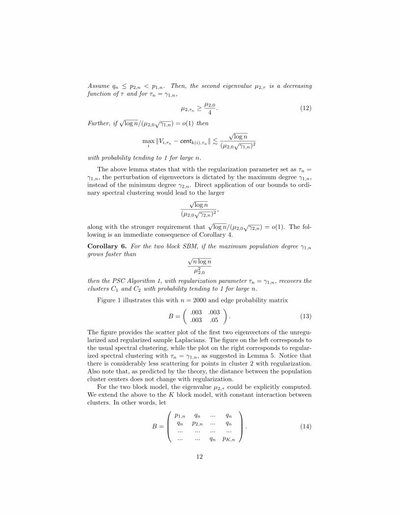
Figure 1: Scatter plot of first two eigenvectors. Here the block probabilitymatrix B is as in (13). Plot a) corresponds to τ = 0, while b) has τ = γ1,n,which in this case is 53. The solid red dot in both plots indicate the populationcluster centers. For each τ , the rows of the sample eigen vector matrix, givenby Vi,τ , are also plotted. The blue ’+’s correspond to the Vi,τ , with nodes i inthe second cluster, while the green circles correspond to the nodes in the firstcluster.

3.1 Improvements In Perturbation Bounds

This subsection uses Theorem 3 to demonstrate improvements, as a result regu-larization, over previous analyses of eigenvector perturbation. In particular, wedemonstrate that for a particular choice of regularization parameter, the depen-dence of the bounds on the minimum degree can be removed. In this subsectionwe assume that the community sizes are equal. While this assumption is notreally needed, it makes the anaylsis considerably less messy.

For the stochastic block model, all nodes in a particular cluster have the sameexpected degree. In the lemma below we consider a two community stochasticblock model. Without loss, assume that each node in cluster 1 has degree γ1,n

that is larger than the degree of nodes in cluster 2, given by γ2,n. Standardresults on spectral clustering provide bounds on the perturbation of the eigen-vectors that are dictated by the minimum degree, which in this case is γ2,n.However, we show that, through regularization, it is dictated by the maximumdegree γ1,n, without any assumption on the magnitude of the minimum degree.

Lemma 5. Consider the two community stochastic block model with

B =

(p1,n qnqn p2,n

).

11

Assume qn ≤ p2,n < p1,n. Then, the second eigenvalue µ2,τ is a decreasingfunction of τ and for τn = γ1,n,

µ2,τn ≥µ2,0

4. (12)

Further, if√

log n/(µ2,0√γ1,n) = o(1) then

maxi‖Vi,τn − centk(i),τn‖ .

√log n

(µ2,0√γ1,n)2

with probability tending to 1 for large n.

The above lemma states that with the regularization parameter set as τn =γ1,n, the perturbation of eigenvectors is dictated by the maximum degree γ1,n,instead of the minimum degree γ2,n. Direct application of our bounds to ordi-nary spectral clustering would lead to the larger

√log n

(µ2,0√γ2,n)2

,

along with the stronger requirement that√

log n/(µ2,0√γ2,n) = o(1). The fol-

lowing is an immediate consequence of Corollary 4.

Corollary 6. For the two block SBM, if the maximum population degree γ1,n

grows faster than √n log n

µ22,0

then the PSC Algorithm 1, with regularization parameter τn = γ1,n, recovers theclusters C1 and C2 with probability tending to 1 for large n.

Figure 1 illustrates this with n = 2000 and edge probability matrix

B =

(.003 .003.003 .05

). (13)

The figure provides the scatter plot of the first two eigenvectors of the unregu-larized and regularized sample Laplacians. The figure on the left corresponds tothe usual spectral clustering, while the plot on the right corresponds to regular-ized spectral clustering with τn = γ1,n, as suggested in Lemma 5. Notice thatthere is considerably less scattering for points in cluster 2 with regularization.Also note that, as predicted by the theory, the distance between the populationcluster centers does not change with regularization.

For the two block model, the eigenvalue µ2,τ could be explicitly computed.We extend the above to the K block model, with constant interaction betweenclusters. In other words, let

B =

p1,n qn ... qnqn p2,n ... qn... ... ... ...... ... qn pK,n

. (14)

12

The number of communities K is assumed to be fixed. Without loss, assumethat p1,n ≥ p2,n . . . ≥ pK,n and let qn < pK,n. We demonstrate that theperturbation of the eigenvectors is dictated by the γK−1,n = di, where i is anynode belonging to cluster K − 1. In other words, it is dictated by the secondsmallest degree, as opposed to the smallest degree.

Lemma 7. Let B be as in (14) and assume qn = o(pK−1,n). If log n/γK−1,n =o(1), then, with τn = γK−1,n the eigenvalue µK,τn is bounded away from zero.Further,

maxi=1,...,n

‖Vi,τn − centk(i),τn‖ .√

log n

γK−1,n.

with probability tending to one as n tends to infinity.

Notice that since |Cmax| � n, the above result, along with Corollary 4, leadsto the following analogue of Corollary 6.

Corollary 8. Let B as in (14) satisfy the assumption of Lemma 7. If γK−1,n

grows at a rate faster than(n log n)1/2,

then, for large n, the PSC Algorithm 1 with τn = γK−1,n, recovers the clusterswith high probability.

Both Lemmas 5 and 7 are proved in Appendix E. It may seem surprisingthat the performance does not depend on the degree of the lowest block, thatis, γK,n. One way of explaining this is that if one can do a good job identifyingthe top K−1 highest degree clusters then the cluster with the lowest degree canalso be identified simply by eliminating nodes not belonging to this cluster. Weremark that the fact that our results do not depend on the minimum degree isnot due to our proof technique, but because of the regularization. Indeed, plotssuch as in Figure 1 demonstrates that the perturbation of eigenvectors dependson the minimum degree with ordinary spectral clustering.

4 Selection Of Strong Clusters

In many practical situations, not all nodes belong to clusters that can be esti-mated well. As mentioned in the introduction, these nodes interfere with theclustering of the remaining nodes in the sense that none of the top eigenvectorsmight discriminate between the nodes that do belong to well-defined clusters.As an example of a real life data set, we consider the political blogs data set,which has two clusters, in Subsection 6.2. With ordinary spectral clustering,the top two eigenvectors do not discriminate between the two clusters. Infact,it is only the third eigenvector that discriminates between the two clusters.This results in bad clustering performance when the first two eigenvectors areconsidered. However, regularization rectifies this problem by ‘bringing up’ theimportant eigenvector, thereby allowing for much better performance.

13

We model the above situation in the following way: Consider a stochasticblock model, as in (14), with K + Kw blocks. In particular, let the blockprobability matrix be given by

B =

(Bs BswB′sw Bw

), (15)

where Bs is a K×K matrix with (p1,n, . . . , pK,n) in the diagonal and qs,n in theoff-diagonal. Further, Bsw, Bw are K×Kw and Kw×Kw dimensional matricesrespectively.

In the above (K+Kw)-block SBM, the top K blocks corresponds to the well-defined clusters, while the bottom Kw blocks corresponds to less well-definedclusters. We refer to the K well-defined clusters as strong clusters. The Kw lesswell-defined clusters are called weak clusters. These are formalized below. Thematrix Bs models the distribution of edges between the nodes belonging to thestrong clusters, while the matrix Bw has the corresponding role for the weakclusters. The matrix Bsw models the interaction between the strong and weakclusters.

We only assume that the rank of Bs is K. Thus, the rank of B is at leastK. We remark that if rank(B) = K, then the model (15) encompasses certaindegree-corrected stochastic block models (see Karrer and Newman [16] for adescription of the model). We provide further remarks on this in Section 8.

As before, we assume that K is known and does not grow with n. The num-ber of weak clusters, Kw, need not be known and is allowed to grow arbitrarilywith n. We do not even place any restriction on the sizes of a weak cluster.Indeed, we even entertain the case that each of the Kw clusters has one node.In other words, the nodes in the weak clusters do not even need to form clusters.

We now formalize our notion of strong and weak clusters. As before, letγ1,n, . . . γK,n denote the degrees of the nodes in the K strong clusters. Forease of analysis, we make the following simplifying assumptions. Assume thatpk,n = pK,n, for each k = 1, . . .K, and that the strong clusters C1, . . . , CK haveequal sizes. Notice that in this case γk,n = γK,n, for k = 1, . . . ,K.

Let bsw and bw be defined as the maximum of the elements in Bsw and Bwrespectively. Denoting by CK+1 the set of nodes belong to a weak cluster, wedefine

γK+1,n = (n− |CK+1|)bsw + |CK+1|bw.The quantity γK+1,n is a bound on the maximum degree of a node in a weakcluster. We make the following assumptions,

γK+1,n

γK,n= o(1). (16)

bsw . bw (17)qs,npK,n

≤ κ < 1, (18)

where κ is a quantity that does not depend on n. Assumption (16) simplystates that the strong clusters have degrees that is of a high order of magnitude

14

than the weak clusters. Assumption (17) states that the interaction betweenthe strong and weak clusters, denoted by bsw, is not too large. More precisely,it is allowed to be at most the same order of bw, which is a proxy of how wellconnected each weak cluster is. Further, Assumption (18) states that, in theabsence of the weak clusters, one can distinguish between the strong clusterseasily.

(a) |CK+1| � n (b) |CK+1| = o(n)

Figure 2: Adjacency matrices for a block model with strong and weak clusters.a) Here n = 2000, with one strong cluster (K = 1) and four weak clusters(M = 4). The first 1000 nodes are taken to belong to the strong cluster 1,while the remaining 1000 nodes were evenly split between the weak clusters2 to 5. The matrix B has diagonal elements (.025, .012, .009, .006, .004) andoff-diagonal element .0025. b) Here n = 2000, two strong clusters (K = 2),three weak clusters (M = 3). The first 1600 nodes are evenly split between thetwo strong clusters, with the remaining nodes split evenly between the weakclusters. The matrix Bs in (15) has diagonal elements .025 and off-diagonalelements .015. The diagonal elements of Bw are taken as (.007, .0071, .0069).The remaining elements of B are taken to be .001.

For a given assignment of nodes in one of the K + Kw clusters, we denoteLτ , Lτ to be the sample, population regularized Laplacians respectively. Asbefore, let µk,τ for k = 1, . . . , n, be the magnitude of the eigenvalues of Lτ ,arranged in decreasing order. Note that µk,τ = 0 for k > K + Kw since Lτ

has rank at most K + Kw. We demonstrate the potential of regularization inremoving the effect of the weak clusters by consider two scenarios, namely, a)|CK+1| � n, and b) |CK+1| = o(n). Example of adjacency matrices drawn fromthese two cases are shown in Figure 2. The following lemma elucidates whythese cases are treated differently.

Lemma 9. The following holds with τn = γK,n:

Claim 1: If |CK+1| � n then µK+1,τn is bounded away from zero, while µK+2,τn

goes to zero for large n.

15

Claim 2: If |CK+1| = o(n) then µK,τn is bounded away from zero, while µK+1,τn

goes to zero for large n.

Lemma 9 states that for regularization parameter τn = γK,n, the eigen gap isbounded away from zero. Here the eigen gap is defined as µK+1,τn−µK+2,τn forthe |CK+1| � n case, while it is taken as µK,τn − µK+1,τn in the |CK+1| = o(n)case. Thus Lemma 9 allows one to control the perturbation of the top K + 1sample eigenvectors in the CK+1 � n case, and the top K eigenvectors inthe CK+1 = o(n) case. Note, since such an eigen gap need not exist in theunregularized case, one may not be able to get perturbation results for the topeigenvectors without regularization.

The next essential ingredient is to demonstrate that with τn = γK,n, thetop population eigenvectors do indeed discriminate between the strong clusters.This is elucidated in Figure 3. The figure deals with the population versionof the adjacency matrix in Figure 2(b), where there are 5 (K = 2 strong,M = 3 weak) clusters. Figures 3(a) and 3(b) show the first 3 eigenvectors of thepopulation Laplacian in the regularized and unregularized cases. We plot thefirst 3 instead of the first 5 eigenvectors in order to facilitate understanding ofthe plot. In both cases the first eigenvector is not able to distinguish between thetwo strong clusters. This makes sense since the first eigenvector of the Laplacianhas elements whose magnitude is proportional to square root of the populationdegrees (see, for example, [28] for a proof of this fact). Consequently, as thepopulation degrees are the same for the two strong clusters, the values for thiseigenvector is constant for nodes belonging to the strong clusters.

The situation is different for the second population eigenvector. In the reg-ularized case, the second eigenvector is able to distinguish between these twoclusters. However, this is not the case for the unregularized case. From Figure3(a), not even the third unregularized eigenvector is able to distinguish betweenthe strong and weak clusters. Indeed, it is only the fifth eigenvector that dis-tinguishes between the two strong clusters in the unregularized case.

The above provides a different perspective on the role of regularization:Regularization is able to bring out the ‘useful’ eigenvectors as the ‘leading’eigenvectors. From hereon we will assume τn = γK,n, unless otherwise specified.

Denote by Vτn the matrix of top K+1 eigenvectors of Lτn . Similarly, denoteby Uτn the matrix of topK eigenvectors of Lτn . Lemma 9 allows us to control theperturbation of Vτn in the |CK+1| � n, and that of Uτn in |CK+1| = o(n) regime.Subsections 4.1 and 4.2 deals with the cases |CK+1| � n and |CK+1| = o(n)respectively.

As before, let k(i) denote the cluster index of node i. In other words, k(i) =k, when i is in cluster Ck, and k = 1, . . . ,K + 1. As before, we use Vi,τn , Ui,τnto denote the i-th row of Vτn , Uτn respectively.

For the |CK+1| � n scenario, Subsection 4.1 provides results showing that therows Vi,τn , for i = 1, . . . , n, are clustered around K+1 points cent1, . . . , centK+1

in RK+1, with the centk’s being well separated. In particular, we show that the

16

(a) Unregularized (b) Regularized

Figure 3: First three population eigenvectors corresponding to the adjacencymatrix in Figure 2(b). In both plots, the x-axis provides the node indices,while the y-axis gives the eigenvector values. The regularization parameter wastaken to be γK,n = 32.4. The shaded blue and pink regions corresponds tothe nodes belonging to the two strong clusters. The solid red line, solid blueline and −×− black lines correspond to the first, second and third populationeigenvectors respectively.

relative perturbation (see Subsection 2.2.2)

pert =maxi=1,...,n ‖Vi,τn − centk(i)‖

min1≤k 6=k′≤K+1 ‖centk − centk′‖(19)

is small. This allows for recovery of the strong clusters C1, . . . , CK , as well asthe set CK+1 using the PSC Algorithm 1.

The |CK+1| = o(n) scenario is addressed in Subsection 4.2. We show thatthere are K well separated points centK1 , . . . , cent

KK in RK so that the relative

perturbation

pert′ =maxi/∈CK+1

‖Ui,τn − centKk(i)‖min1≤k 6=k′≤K ‖centKk − centKk′‖

(20)

is small. In other words, the rows of the matrix Uτn that are not in CK+1 areconcentrated around the centKk ’s. Note, since we say nothing about the nodesin CK+1, this result is in a sense weaker than that in Subsection 4.1. However,since we are dealing with the situation where the size of CK+1 is small comparedto n, this is not expected to have a significant impact on clustering.

The following quantity will appear as a bound on the perturbation of eigen-vectors.

δn =1

√γK,n

max

{√log n√γK,n

,γK+1,n

γK,n

}(21)

Notice that δn goes to zero if γK,n grows faster than log n.

4.1 |CK+1| � n

Lemma 9 demonstrates that with τn = γK,n there is a gap between the K+1-thand K + 2-th smallest eigenvalues, given by µK+1,τn and µK+2,τn respectively.

17

This eigen gap allows us to characterize the perturbation of the first K + 1eigenvectors of Lτn . In particular, we demonstrate that with the first K + 1eigenvectors of the sample Laplacian matrix Lτn one can reliably recover thestrong clusters. In essence, the eigenvectors treat CK+1 as one composite cluster.Theorem 10, below, describes our results.

Theorem 10. Assume log n/γK,n = o(1) and τn = γK,n. Then, there existsK + 1 points cent1, . . . , centK+1 in RK+1 with

‖centk′ − centk‖ =

√1

|Ck|+

1

|Ck′ |for k′ 6= k (22)

so thatmax

i=1,...,n‖Vi,τn − centk(i)‖ . δn. (23)

with probability tending to one for large n. Here δn is as in (21).

As mentioned earlier, we only wish to identify between the nodes in thestrong clusters. The corollary below states the result for recovery of the strongclusters, as well as a CK+1. In Step 2 of Algorithm 1, we set Algorithm 2 tooutput K + 1 clusters and take

t =min1≤k 6=k′≤K+1 ‖centk′ − centk‖

2.

We have the following.

Corollary 11. If√nδn = o(1), then with τn = γK,n, the PSC Algorithm 1

recovers the strong clusters C1, . . . , CK , as well as the cluster CK+1, with prob-ability tending to one for large n.

The above follows from (22) and (23), and using the fact that |Ck| � n foreach k. Consequently, pert .

√nδn, where pert is given by (19). The result is

completed using Lemma 2.Example sizes of γK,n and γK+1,n for the condition in Corollary 11 to hold

are:

1. γK,n grows linearly with n, while γK+1,n is o(n).

2. γK,n grows faster than√n log n, while γK+1,n is O(n1/4(log n)3/4)

Figure 4 illustrates the above theorem. Here, K = 1 and M = 4. Since thefour weak clusters are relatively indistinguishable, as can be seen from Figure2(a), we only wish to separate the strong cluster from the set of weak clus-ters. Figure 4 shows the scatter plot of the first two eigenvectors of the sampleLaplacian matrices. Without regularization, the rows of the eigenvector matrixcorresponding to the weak clusters are fairly spread out, as can be seen fromFigure 4(a). With regularization, these rows are less spread out, as predictedfrom the above results. This is shown in Figure 4(b). Indeed, running k-means,with k = 2, on the above resulted in a mis-classification of 9.2% of the nodes inthe unregularized case, compared with only 1.6% in the regularized case.

18

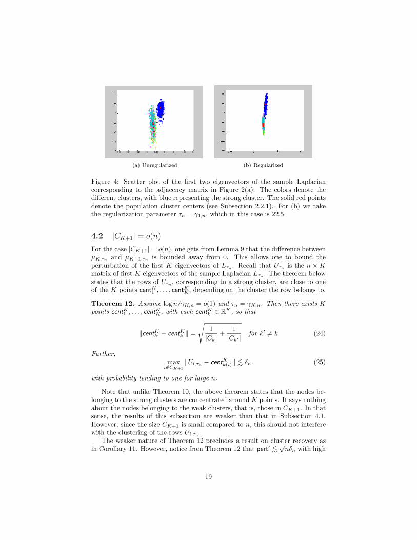
(a) Unregularized (b) Regularized

Figure 4: Scatter plot of the first two eigenvectors of the sample Laplaciancorresponding to the adjacency matrix in Figure 2(a). The colors denote thedifferent clusters, with blue representing the strong cluster. The solid red pointsdenote the population cluster centers (see Subsection 2.2.1). For (b) we takethe regularization parameter τn = γ1,n, which in this case is 22.5.

4.2 |CK+1| = o(n)

For the case |CK+1| = o(n), one gets from Lemma 9 that the difference betweenµK,τn and µK+1,τn is bounded away from 0. This allows one to bound theperturbation of the first K eigenvectors of Lτn . Recall that Uτn is the n × Kmatrix of first K eigenvectors of the sample Laplacian Lτn . The theorem belowstates that the rows of Uτn , corresponding to a strong cluster, are close to oneof the K points centK1 , . . . , cent

KK , depending on the cluster the row belongs to.

Theorem 12. Assume log n/γK,n = o(1) and τn = γK,n. Then there exists Kpoints centK1 , . . . , cent

KK , with each centKk ∈ RK , so that

‖centKk′ − centKk ‖ =

√1

|Ck|+

1

|Ck′ |for k′ 6= k (24)

Further,maxi/∈CK+1

‖Ui,τn − centKk(i)‖ . δn. (25)

with probability tending to one for large n.

Note that unlike Theorem 10, the above theorem states that the nodes be-longing to the strong clusters are concentrated around K points. It says nothingabout the nodes belonging to the weak clusters, that is, those in CK+1. In thatsense, the results of this subsection are weaker than that in Subsection 4.1.However, since the size CK+1 is small compared to n, this should not interferewith the clustering of the rows Ui,τn .

The weaker nature of Theorem 12 precludes a result on cluster recovery asin Corollary 11. However, notice from Theorem 12 that pert′ .

√nδn with high

19

probability, where pert′ as in (20). Consequently, if we take

t =min1≤k 6=k′≤K ‖centKk′ − centKk ‖

2

in Algorithm 2 then one has that for nodes i and j in strong clusters, ‖Ui,τn −Uj,τn‖ < t iff i and j belong to the same strong cluster. Thus, the nodes in thestrong clusters are well separated.

(a) Unregularized (b) Regularized

Figure 5: Second sample eigenvector corresponding to situation in Figure 3. Asbefore, in both plots, the x-axis provides the node indices, while the y-axis givesthe eigenvector values. As before, the shaded blue and pink regions correspondsto the nodes belonging to the two strong clusters. For plots (a) & (b) the blueline correspond to the second eigenvector of the respective sample Laplacianmatrices.

In Figure 5(a) and 5(b) we show the second sample eigenvector for the twocases in Figure 3(a) and 3(b). Note, we do not show the first sample eigenvectorsince from Figure 3(a) and 3(b), the corresponding population eigenvectors arenot able to distinguish between the two strong clusters. As expected, it is onlyfor the regularized case that one sees that the second eigenvector is able to do agood job in separating the two strong clusters. Running k-means, with k = 2,resulted in a mis-classification of 49% of the nodes in the strong clusters in theunregularized case, compared with 16.25% in the regularized case.

5 Comparison With Regularization In [9], [7]

In Dasgupta et al. [9], Chaudhuri et al. [7], the following alternative regularizedversion of the symmetric Laplacian is proposed:

Ldeg,τ = D−1/2τ AD−1/2

τ . (26)

Here, the subscript deg stands for ‘degree’ since the regular Laplacian is modifiedby adding τ to the degree matrix D. Notice that for the PSC algorithm, thematrix A in the above expression was replaced by Aτ .

20

Borrowing from results on the concentration of random graph Laplacians[23], we were able to show concentration results (11) for the regularized Lapla-cian in the PSC algorithm. This result does not require any assumption onthe minimum degree, provided τmin & log n. It was shown in Qin and Rohe[24] that analogous concentration results also hold for the regularized Lapla-cian Ldeg,τ . This was shown for the more general degree corrected stochasticblock model [16]. However, an analysis of the eigen gap of Ldeg,τ (or its pop-ulation version), as a function of the regularization parameter, was not givenin these works. Consequently, it is unclear at this stage whether the benefitsof regularization, resulting from the trade-offs between the eigen gap and theconcentration bound, as demonstrated in Subsection 3.1 and Section 4 for thePSC algorithm, also hold for the regularization in [7], [24].

Further, it is conjectured in [7], [24] that the regularization parameter takento be the average degree should be optimal in balancing the bounds. However,for the situation in Lemma 7, the average degree can be too large, especiallywhen there are clusters with very high degree. Indeed, for the K block modelconsidered in Lemma 7, our proof technique also shows that if τ grows fasterthan γK−1,n then the smallest eigenvalue of Lτ goes to 0 for large n. We believethe same to hold true for the regularization (26) as well.

6 Data dependent choice of τ

For the results in Subsection 3.1 and Section 4, the regularization parameterdepended on a population quantity which is not known in practice. Here, wepropose a data dependent scheme to select the regularization parameter. Wealso compare it with another scheme that uses the Girvan-Newman modularity[6] . This was suggested in [8]. We use the normalized mutual informationcriterion (NMI) [2], [29], to quantify the performance of the spectral clusteringalgorithm in terms of closeness of the estimated clusters to the true clusters.The NMI is a widely used measure of closeness of the estimated clusters to thetrue clusters.

We now describe our proposed scheme: Our theoretical bounds provide ameans to select the regularization parameter τ . One possible route would be toconsider the statistic √

max{τ, dmin} µK,τ .

Here dmin is the minimum degree of the realized graph and µK,τ is K-th small-est eigen value of the sample Laplacian Lτ . From bound (7), it appears thatfinding the τ that maximizes this criterion should provide a good estimate ofthe optimum τ . However, the above criterion does not perform well when theaverage degree of the graph is low, most likely due to the fact the µK,τ is apoor substitute for its population counterpart. An alternative criterion, whichperforms much better, is obtained by directly estimating the quantity in (10).

In particular, for each τ in grid, an estimate Lτ of Lτ is obtained using clusteroutputted from the PSC algorithm using that τ . Here, the estimate Lτ is the

21

population Laplacian corresponding to an edge probability matrix P , as in (1),with an estimated block probability matrix B. In particular, the (k1, k2)-thentry of B is taken to be the proportion of edges between the nodes in theestimates of the clusters k1 and k2 with the given τ . The following statistic isthen considered:

DK−estτ =‖Lτ − Lτ‖

µK

(Lτ

) , (27)

where µK

(Lτ

)denotes the the K-th smallest eigenvalue of Lτ . The τ that

minimizes the DK − estτ criterion is then chosen. Since this criterion providesan estimate of the Davis-Kahan bound, we call it the DK-est criterion.

We compare the above to the scheme that uses Girvan-Newman modularity[6], [21], as suggested in [8]. For a particular τ in the grid, the Girvan-Newmanmodularity is computed for the clusters outputted using the PSC algorithmapplied with that τ . The τ that maximizes the modularity value over the gridis then chosen.

Notice that the best possible choice of τ would be the one that simply max-imizes the NMI over the selected grid. However, this cannot be computed inpractice since calculation of the NMI requires knowledge of the true clusters.Nevertheless, this provides a useful benchmark against which one can comparethe other two schemes. We call this the ‘oracle’ scheme.

6.1 Simulation Results

Figure 6 provides results comparing the two schemes. We perform simulationsfollowing the pattern of [2]. If particular, for a graph with n nodes we take theK clusters to be of equal sizes. The K ×K block probability matrix is taken tobe of the form

B = fac

βw1 1 ... 1

1 βw2 ... 1... ... ... ...... ... 1 βwK

.

Here, the vector w = (w1, . . . , wK), which are the inside weights, denotes therelative degrees of nodes within the communities. Further, the quantity β, whichis the out-in ratio, represents the ratio of the probability of an edge betweennodes from different communities to that of probability of edge between nodes inthe same community. The parameter fac is chosen so that the average expecteddegree of the graph is equal to λ. In the graphs of Figure 6, we denote β and was OIR and InWei respectively.

Figure 6 compares the two methods of choosing the best τ for various choicesof n, K, OIR, InWei and λ. In general, we see that the DK − est selectionprocedure performs at least as well, and in some cases much better, than theprocedure that used the Girvan-Newman modularity. The performance of thetwo methods is much closer when the average degree is small.

22

0 10 20 30 40 50 600.5

0.55

0.6

0.65

0.7

NM

I

Regularization parameter

NM

I

Girv

an−N

ewm

an

DK

−est

n = 2000 K = 4

λ = 30.0 OIR = 0.65

InWei = [1 1 5 10 ]

0 10 20 30 40 50 600

0.5

1

1.5

2

NMIGirvan−NewmanDK−est

0 10 20 30 40 50 600.6

0.7

0.8

0.9

NM

I

Regularization parameter

NM

I

Girv

an−N

ewm

an

DK

−est

n = 1200 K = 3

λ = 30.0 OIR = 0.70

InWei = [1 5 5 ]

0 10 20 30 40 50 600

0.5

1

1.5

NMIGirvan−NewmanDK−est

0 5 10 15 20 25 30 35 400.6

0.7

0.8

0.9

NM

I

Regularization parameter

NM

I

Girv

an−N

ewm

an

DK

−est

n = 1200 K = 3

λ = 20.0 OIR = 0.50

InWei = [1 5 5 ]

0 5 10 15 20 25 30 35 400

0.5

1

1.5

NMIGirvan−NewmanDK−est

0 2 4 6 8 10 12 14 16 18 200

0.5

1

NM

I

Regularization parameter

NM

I

Girv

an−N

ewm

an

DK

−est

n = 2000 K = 4

λ = 10.0 OIR = 0.10

InWei = [1 5 5 10 ]

0 2 4 6 8 10 12 14 16 18 200

2

4

NMIGirvan−NewmanDK−est

Figure 6: Performance of spectral clustering as a function of τ for stochasticblock model for λ values of 30, 20 and 10. The right y-axis provides values forthe Girvan-Newman modularities and DK est functions, while the left y-axisprovides values for the normalized mutual information (NMI). The 3 labeleddots correspond to values of the NMI at τ values which minimizes the DK-est,and maximizes the Girvan-Newman modularity and the NMI. Note, the oracleτ , or the τ that maximizes the NMI, cannot be calculated in practice.

6.2 Analysis Of A Real Dataset

We also studied the efficacy of our procedure on the well studied network ofpolitical blogs [1]. The data set aims to study the degree of interaction betweenliberal and conservative blogs over a period prior to the 2004 U.S PresidentialElection. The nodes in the networks are select conservative and liberal blogsites. While the original data set had directed edges corresponding to hyperlinksbetween the blog sites, we converted it to an undirected graph by connectingtwo nodes with an edge if there is at least one hyperlink from one node to the

23

Figure 7: Performance of the three schemes for the political blogs data set [1].

other.

(a) Unregularized (b) Regularized (τ = 2.25)

Figure 8: Second eigenvector of the unregularized and regularized Laplacians forthe political blogs data set [1]. The shaded blue and pink regions correspondsto the nodes belonging to the liberal and conservative blogs respectively.

The data set has 1222 nodes with an average degree of 27. Simple spectralclustering, that is with τ = 0, resulted in only 51% of the nodes correctlyclassified as liberal or conservative. The oracle procedure, with τ = 0.5, resultedin 95% of the nodes correctly classified. The DK-est procedure selected τ =2.25, with an accuracy of 81%. The Girvan-Newman procedure, in this case,outperforms the DK-est procedure, providing the same accuracy as the oracleprocedure. Figure 7 illustrates these findings.

The results of Section 4 also explain why unregularized spectral clusteringperforms badly. The first eigenvector in both cases (regularized and unregular-ized) does not discriminate between the two clusters. In Figure 8, we plot thesecond eigenvector of the regularized and unregularized Laplacians. The secondeigenvector is able to discriminate between the clusters in the regularized case,while it fails to do so in without regularization. Indeed, it is only the third

24

Figure 9: Third eigenvector of the unregularized Laplacian.

eigenvector in the unregularized case that distinguishes between the clusters, asshown in Figure 9.

7 Proof Techniques

Here we discuss the high-level idea behind the proofs of the various theorems.We first discuss the proof of Theorem 3.

7.1 Proof Of Theorem 3

The theorem provides a high-probability bound on

‖Vi,τ − Vi,τ‖, (28)

which is the `2-norm of the difference of the i-th row of the sample and popula-tion eigenvectors. From the Davis-Kahan theorem [5], one can get the followingbound on the difference of sample and population eigenvector matrices:

‖Vτ − Vτ‖ .‖Lτ −Lτ‖

µK,τ

Further, from recent results on concentration of Laplacian of random graphs[23], [19], one gets that ‖Lτ − Lτ‖ .

√log n/

√τmin with high probability.

Consequently,

‖Vτ − Vτ‖ .√

log n

µK,τ√τmin

with high probability. (29)

Using the fact that‖Vi,τ − Vi,τ‖ ≤ ‖Vτ − Vτ‖,

one can infer that the right side of (29) provides a bound on (28) as well.However, the above bound it too weak to make inferences about cluster recovery.Consequently, we strengthen these bounds by demonstrating that

‖Vi,τ − Vi,τ‖ .√

log n

(µK,τ√τmin)2

with high probability. (30)

25

These improvements arise from the extension of the techniques in [3] to normal-ized Laplacians. We now briefly describe the technique.

For convenience, we remove the subscript τ from the various quantities. LetM = diag(λ1, . . . , λK) denote the diagonal matrix of top K eigenvalues of L ,where |λ1| ≥ . . . ≥ |λK | > 0. Notice that µk,τ = |λk|. Further, let M bethe corresponding matrix for L. We use the symbol ∆ to denote the differenceof a sample and population quantity. In particular, let ∆L = L − L and∆V = V − V . Using LV = V M , note that

V − V = LV M−1 − V

= (L + ∆L)(V + ∆V )M−1 − V

Consequently, using L V = V M , one has from the above

V − V = ∆LV M−1 + (L + ∆L)∆V M−1 + V (M − M)M−1 (31)

In Appendix A, in particular Lemma 14, we provide deterministic bounds onthe `2-norm of the i-th row of each of three terms in the right side of (31). Thesebounds are applicable to the difference of top-K eigenvector matrices of any twoLaplacian matrices. Assuming an SBM framework, Appendix B provides highprobability bounds on each of the three terms in (31).

7.2 Proof Of Results In Section 4

We prove in Lemma 19, Appendix C, that with regularization parameter τn =γK,n, the Laplacian matrix Lτn is close to a rank K + 1 Laplacian matrix

Lτn in spectral norm. Here Lτ is the population regularized Laplacian of aK + 1-block SBM constructed from clusters C1, . . . , CK and CK+1, and blockprobability matrix

B =

(Bs bsw1

bsw1′1′ bw

),

where the K ×K matrix Bs, and the quantities bsw, bw are as in (15). Since Bhas rank K+1, the same holds also for Lτ . We denote by µk,τ , for k = 1, . . . , n,

to be the magnitude of the eigenvalues of Lτ arranged in decreasing order.Notice that µk,τ = 0 for k > K + 1. Explicit expressions for the non-zero

eigenvalues of Lτ are given in Lemma 21, Appendix C.4.Consequently, from Lemma 19 one get that the eigenvalues of Lτn are close

to that of Lτn via Weyl’s inequality [5]. Lemma 9 follows from examining theeigenvalues of Lτn , as given in Lemma 21.

In the next subsection we provide the idea behind the proof of Theorem 10.The proof of Theorem 12, although slightly more involved, is similar in spirit.We leave its proof completely to Appendix C.3.

7.2.1 Proof Of Theorem 10

Let Vτn be the n× (K+ 1) matrix corresponding to the first K+ 1 eigenvectorsof the population Laplacian Lτn . Recall that Vτn is the sample version of Vτn .

26

Further, denote by Vτn as the n × (K + 1) matrix corresponding to the firstK + 1 eigenvectors of Lτn .

Since Lτn is the population Laplacian of a K + 1-block SBM, the matrixVτn has K + 1 distinct rows, with the unique rows corresponding to the K + 1clusters. Take these distinct rows as cent1, . . . , centK+1. Then (22) follows fromLemma 1.

As mentioned in Subsection 2.2, since there are multiple choices of Vτn andVτn , we take Vτ to be the eigenvector matrix of Lτn that is closest to Vτn inspectral norm. With Vτn so defined, we take Vτn to be eigenvector matrix ofLτn that is analogously closest to Vτn .

Theorem 10 follows from Theorem 13 below, which is proved in AppendixC.2. It demonstrates that for a particular choice of regularization parameter τn,not only is Vi,τn close to its population counterpart Vi,τn , but also Vi,τn is close

to Vi,τn . As before, the subscript i denotes the i-th row of these matrices.

Theorem 13. For the regularization parameter τn = γK,n, we have

‖Vi,τn − Vi,τn‖ .1

√γK,n

γK+1,n

γK,n(32)

Further, if log n/γK,n = o(1) then,

maxi‖Vi,τn − Vi,τn‖ .

√log n

γK,n(33)

with probability tending to one for large n.

The claim (32) uses the result that Lτn is close to Lτn for τn = γK,n. This

leads to the fact that the eigenvector matrices Vτn and Vτn are also close. Theclaim (33) follows from Theorem 17, which is a slightly more general versionof Theorem 3. The improvements in the Davis-Kahan bounds are essentialingredients in the proofs of both (32) and (33).

Proof of Theorem 10. Recall that cent1, . . . , centK+1 are taken to be the K + 1distinct rows of Vτn , with centk corresponding to cluster Ck. The proof of (22)follows from Lemma 1.

Theorem 13 states that if the bounds (32) and (33) are small, then therows of sample eigenvector matrix Vτn are concentrated near one of the K + 1distinct points representing the clusters C1, . . . , CK+1. Correspondingly, (23)follows from using

‖Vi,τn − Vi,τn‖ ≤ ‖Vi,τn − Vi,τn‖+ ‖Vi,τn − Vi,τn‖.

27

8 Discussion

The paper is an attempt to provide a theoretical quantification for regulariza-tion in spectral clustering. Increasing the regularization parameter makes thesample Laplacian better concentrated around its corresponding population ver-sion. However, increasing the regularization parameter also changes the eigengap of the population Laplacian. This was also noticed in [7], [24] for a differentform of regularization. The larger this gap, the better is cluster recovery. Intu-itively, this gap should be small for large τ as the population Laplacian becomesmore like a constant matrix. Consequently, the best choice of regularization pa-rameter is the one that balances these two competing effects. Sections 3 and4 demonstrate two different ways in which regularization affects this gap. Tothe best of our knowledge, this is the first paper that incorporates both theseeffects in the quantification of regularization.

In Subsection 3.1, where the goal was to recover all the clusters, the regu-larization τn = γK−1,n was chosen since

µK,τ � µK,0 for τ . γK−1,n

In other words, the eigen gap at τn is the same order of magnitude as that atτ = 0. Consequently, the regularization parameter τn increases the performanceof clustering since the sample Laplacian Lτ is better concentrated around itspopulation version at τ = τn. Our proof technique also shows that for anyalternative larger choice of regularization parameter, say τ ′n, with τn = o(τ ′n),the eigen gap µK,τ ′

ngoes to zero for larger n. For the two block model it can

even be shown that such a choice would lead to worse bounds. Consequently,this also hints that for the regularization in [7], [24], the regularizer set as theaverage degree, as conjecture in [24], is not the best choice, especially whenthere is large variability in the degrees. However, when the degrees are more orless equal we believe that the average degree should work well since it is closeto γK−1,n.

More importantly, in Section 4 we show that regularization can help in situa-tions where not all nodes belong to well defined clusters. In such situations, theimprovements via regularization are due to two reasons. The first, as mentionedabove, is due to better stability of sample Laplacian around its correspondingpopulation counterpart. The second, as demonstrated in Lemma 9, is throughthe creation of a gap between the top few eigenvalues and the remaining. Inthis regard, we considered two different regimes depending on the size of theset of nodes belonging to the weak clusters. We also demonstrate in Subsection4.1 and 4.2, that the top few population eigenvectors are able to distinguishbetween the nodes of the strong clusters with regularization. This need not bethe case without regularization, as illustrated in Figure 3. We also demonstratethis on the political blogs data set.

As remarked in Section 4, if the rank of B, given by (15), is K then themodel encompasses specific degree-corrected stochastic block models (D-SBM)[16]. In particular, consider a K-block D-SBM, with degree weight parameterfor node i to be θi, where 0 < θi ≤ 1. Assume that θi = 1 for a large number

28

of nodes. Take the nodes in the strong clusters to be those with θi = 1. Thenodes in the strong clusters are associated to one of K clusters depending on thecluster they belong to in the D-SBM. The remaining nodes are taken to be inthe weak clusters. Assumptions (16), (17) and (18) puts constraints on the θi’swhich allows one to distinguish between the strong clusters via regularization.

From the results of Section 4, a high value of regularization parameter re-duces the influence of the less well defined clusters. We conjecture that theseresults also extend to situations where there is a hierarchy of clusters. In thiscase, the less well defined clusters would correspond to those lower down in thehierarchy. An natural way of going about this is to cluster in a hierarchicalfashion, using larger values of τ for clusters higher up in the hierarchy. In thisregard, there seems to be parallels between this approach and the clustering ofpoints using the level-set approach [13]. We hope to investigate this in a futurework.

We provide a data dependent technique for choosing the regularization pa-rameter τ , and compare it the scheme that uses the Girvan-Newman modularity.Since the DK-est technique compares the perturbation of the sample Laplacianto the population Laplacian of a stochastic block model, chosen based on theselected clusters, the procedure is similar in spirit to modularity based methodssuch as Girvan-Newman modularity. From our simulations, our method is seento perform better than the Girvan-Newman scheme. For the application to thepolitical blogs data set our scheme performs well. However, the scheme thatuses the Girvan-Newman modularity outperforms our scheme, most likely dueto the large variance in the degrees of the nodes for this dataset. We believethat one can obtain a degree-corrected version of our scheme which performsbetter in such situations. We leave this for a future work.

Acknowledgments

This work was partly supported by ARO grant W911NF-11-1-0114. We wouldlike to thank Sivaraman Balakrishnan for some very helpful discussions regard-ing strengthening of the Davis-Kahan bounds. A. Joseph would also like tothank Purnamrita Sarkar for very helpful discussions regarding the results inSection 4, and also Arash A. Amini for sharing the code used in the work [2].

A Bounds On Eigenvectors Differences

In this section we provide deterministic bounds on the difference of eigenvectorsfrom two arbitrary Laplacians matrices. This will be used to provide highprobability bounds on the perturbation of eigenvectors. In particular, considerany two Laplacian matrices,

L = D−1/2AD−1/2

L = D−1/2PD−1/2,

29

where A, D are the adjacency matrices and the diagonal matrix of degreescorresponding to L. By adjacency matrix we refer to any symmetric matrixwith entries in [0, 1]. Similarly P, D are the analogous quantities for L .

Denote,D = diag(d1, . . . , dn) and dmin = min

idi.

Let V, V be the n×K ′ eigenvector matrices corresponding to top (in absolutevalue) K ′ eigenvalues of L, L respectively. As mentioned in Subsection 2.2,since there are multiple choices for V and V , for a given choice of V , we takeV as the eigenvector matrix of L that is closest to V in spectral norm. Wealso denote by ρ1,K′ and ρ2,K′ the K ′-th smallest eigenvalue (in magnitude) ofL and L respectively.

Denote the i-th row of the above eigenvector matrices as Vi and Vi. In thissection we provide deterministic bounds on ‖∆Vi‖, where

∆Vi = Vi − Vi.

In general, we use the symbol ∆ to denote the difference of two quantities. Forexample ∆A = A − P and ∆V = V − V . We also use the the subscript i∗ todenote the i-th row of a matrix. The following inequality will be use frequentlyin the analysis: For matrices H1, H2

‖H1H2‖ ≤ ‖H1‖‖H2‖ (34)

The lemma below provides deterministic bounds on the `2 norm of each rowof ∆V , given by ∆Vi. Our proof technique involves generalization of perturba-tion bounds obtained in [3] for eigenvectors of the unnormalized Laplacian, tothat of the normalized Laplacians.

Lemma 14. The following bound holds:

‖∆Vi‖ ≤b1,i

ρ1,K′+

b2,i‖∆V ‖ρ1,K′

+b3,i

ρ1,K′, (35)

where,

b1,i = Ri ‖Li∗‖ ‖∆RV ‖+ |∆Ri| ‖Vi‖

+(Ri ‖∆Ai∗‖ ‖∆RV ‖+Ri

∥∥∥∆Ai∗D−1/2V

∥∥∥) /√dmindi (36)

b2,i = ‖Li∗‖ (1 +Ri ‖∆R‖+ |∆Ri|) +‖R‖ ‖∆Ai∗‖√

dmindi(37)

b3,i = ‖Vi‖‖∆L‖. (38)

Here R = diag(R1, . . . , Rn) is (D/D)1/2. Further, ∆R = diag(∆R1, . . . ,∆Rn),where ∆R = R− I.

30

Proof. Let M1 = diag(λ1, . . . , λK′) denote the diagonal matrix of eigenvectors ofL, where |λ1| ≥ . . . ≥ |λK′ |. Notice that ρ1,K′ = λK′ . Let M2 be the analogousdiagonal matrix of eigenvalues of L . Now,

∆V = LVM−11 − V

= L(V + ∆V )M−11 − V (39)

The first equality follows from noticing that LV = VM1, since the columns ofV are eigen vectors

Correspondingly, from (39) one gets that ∆V is the sum of three terms givenby,

∆V = [L + ∆L]V M−11 + [L + ∆L]∆VM−1

1 − V (40)

Notice that L V = V M2. Consequently, from (40) one gets the ∆Vi is the sumof three 1×K ′ row vectors J1, J2, J3, where

∆Vi = ∆Li∗V M−11︸ ︷︷ ︸

J1

+ [Li∗ + ∆Li∗]∆VM−11︸ ︷︷ ︸

J2

+ Vi(M2 −M1)M−11︸ ︷︷ ︸

J3

(41)

Below, we provide bounds on the `2 norm each of the above three separately.These would correspond to the three terms appearing in the right side of (35).Before this, we describe how we handle the ∆Li∗ term appearing in (41).

Notice that,

∆L = RD−1/2AD−1/2R−L

= RLR−L︸ ︷︷ ︸∆L1

+RD−1/2∆AD−1/2R︸ ︷︷ ︸∆L2

(42)

By subtracting and adding RL , write ∆L1 = ∆L11 + ∆L12, where

∆L11 = RL ∆R (43)

∆L12 = ∆RL (44)

Similarly ∆L2 = ∆L21 + ∆L22, where

∆L21 = RD−1/2∆AD−1/2∆R

∆L22 = RD−1/2∆AD−1/2

We now bound the `2-norm of the three terms in (41). We first bound the`2-norm of J1. Notice that,

‖∆L11i∗V M

−11 ‖ ≤ Ri‖Li∗‖‖∆RV ‖‖M−1

1 ‖

and‖∆L12

i∗V M−11 ‖ ≤ |∆Ri|‖Vi‖‖M2M

−11 ‖,

where for the above we use that L V = V M2. Similarly,

‖∆L21i∗V M

−11 ‖ ≤ Rid

−1/2i d

−1/2min ‖∆Ai∗‖‖∆RV ‖‖M−1

1 ‖

31

and‖∆L22

i∗V M−11 ‖ ≤ Rid

−1/2i d

−1/2min ‖∆Ai∗D

−1/2V ‖‖M−11 ‖

The expression for b1,i results from using ‖M−11 ‖ = 1/ρ1,K′ and ‖M2M

−11 ‖ ≤

1/ρ1,K′ .Similarly for `2 norm of J2, notice that it is bounded by

(‖Li∗‖+ ‖∆Li∗‖) ‖∆V ‖‖M−11 ‖

We need to bound ‖∆Li∗‖. From the above one sees that,

‖∆L11i∗ ‖ ≤ Ri‖Li∗‖ ‖∆R‖

‖∆L12i∗ ‖ ≤ |∆Ri| ‖Li∗‖

‖∆L2i∗‖ ≤ ‖R2‖ ‖∆Ai∗‖/

√didmin

The claim for the `2 norm of J3 follows from using the fact that

‖M2 −M1‖ ≤ ‖∆L‖,

which follows from Weyl’s inequality [5].

In equation (35), one needs to provide an upper bound on ‖∆V ‖ in (35).This is achieved using the Davis-Kahan theorem (see, for example, [5]), a versionof which we state below. Recall that ρ2,K′ denoted the K ′-th smallest eigenvalueof L . Similarly, denote as ρ2,K′+1 the K ′+1 smallest eigenvalue (in magnitude)of L . We remark that if L corresponds to the population Laplacian of K ′ blockSBM, then ρ2,K′+1 = 0. However, here we made no such assumption on L .

Theorem 15 (Davis-Kahan with spectral norm). Let ‖∆L‖ < (ρ2,K′−ρ2,K′+1)/2.Then

‖∆V ‖ ≤ 2‖∆L‖

ρ2,K′ − ρ2,K′+1. (45)

The following is an immediate corollary of the above and Lemma 14.

Corollary 16. If ‖∆L‖ ≤ (ρ2,K′ − ρ2,K′+1)/2 then

‖∆Vi‖ ≤2b1,i

ρ2,K′+

4b2,i‖∆L‖ρ2,K′(ρ2,K′ − ρ2,K′+1)

+2b3,i

ρ2,K′. (46)

Here b1,i, b2,i and b3,i are as in Lemma 14.

Proof. Notice that |ρ2,K′ − ρ1,K′ | ≤ ‖∆L‖ using Weyl’s inequality (see for ex-ample [5]). Consequently, ρ1,K′ ≥ ρ2,K′/2 since ‖∆L‖ ≤ ρ2,K′/2. The proof iscompleted using Theorem 15.

32

B Proof of Theorem 3

We apply the results of Appendix A, in particular Corollary 16, to prove a moregeneral version of Theorem 3, which we describe below. This will be requiredin the proof of Theorem 13.

Consider a K block SBM as in Section 3. In Theorem 17 we use Corollary 16to bound the perturbation of the first K ′ eigenvectors of the sample Laplacianmatrix. Taking K ′ = K leads to Theorem 3.

In the theorem below we use the notation Appendix A with L = Lτ and L =Lτ . We take V, V in Appendix A to be the eigenvector matrices correspondingto the first K ′ eigenvectors, where K ′ ≤ K, of L, L respectively. In this caseρ2,K′ = µK′,τ and ρ2,K′+1 = µK′+1,τ . We also require the following moregeneral version of Assumption 2, which given the size of the eigen gap as afunction of τ .

Assumption 3 (Eigen gap).

ρ2,K′ − ρ2,K′+1 > 20

√log n√τmin

Notice that with K ′ = K, Assumption 3 is the same as Assumption 2 sinceρ2,K′+1 = 0 for the K block SBM. Then we have the following:

Theorem 17. Let Assumptions 1 and 3 hold. Then, with probability at least1− (2K ′ + 5)/n,

maxi‖Vi − Vi‖ ≤

δτ,nρ2,K′(ρ2,K′ − ρ2,K′+1)

(47)

where

δτ,n = 293

√log n

τmin+ 31

√log n√τmin

‖Vi‖+ 12K ′√

log n

τ3/2min

. (48)

Proof of Theorem 3. Take K ′ = K in Theorem 17. As mentioned before, in thiscase Assumption 3 is the same as Assumption 2 since ρ2,K′+1 = µK+1,τ = 0.Further, ‖Vi‖ = 1/

√|Ck(i)| from Lemma 22.

We now prove Theorem 17. Notice that D = diag(d1,τ , . . . , dn,τ ) andD = diag(d1,τ , . . . , dn,τ ). Let τmin = max(τ, dmin) satisfy the condition inAssumption 1. In other words, recall that

τmin = κn log n,

where κn > c = 32. Further, let

τi = max{τ, di}. (49)

We prove Theorem 17 by appealing to Corollary 16. To do this, the follow-ing deterministic as well as high probability bounds that are derived in theSubsections D.1 and D.2 in Appendix D would prove to be useful.

33

Deterministic bounds: With L = Lτ , one has

‖Pi∗‖ ≤√di,τ and ‖Li∗‖ ≤ 1/

√τmin.

High Probability bounds: We assume that c2 is a positive number satisfying

c2/√c < 1.

Let

c1 = .5c22/(1 + c2/√c). and c3 = c2/

√1− c2/

√c

From Subsection D.2, the following holds with probability at least 1 − (2K ′ +3)/nc1−1: For each i = 1, . . . , n,

1.

|∆Ri| ≤ c3√

log n√τi

(50)

2.

‖∆Ai∗D−1/2V ‖ ≤ c2K ′√

log n

τmin(51)

3.‖∆Ai∗‖2 ≤ di,τ + c2

√τi log n (52)

Notice that (50) implies that Ri ≤ 1 + c3/√c, using c log n ≤ τi. Further, (52)

implies that‖∆Ai∗‖2 ≤ (1 + c2/

√c)di,τ ,

using τi, as well as c log n, are at most di,τ .For convenience we take c = 32, c2 = 2

√2. Then one has c1 > 2, c3 = 4

√2.

The following lemma shows that the condition of Corollary 16 is satisfied withhigh probability.

Lemma 18. Let Assumption 1 be satisfied and let c, c2 be chosen as above.Then with probability at least 1− 2/nc1−1, the following hold

‖∆L‖ ≤ κ√

log n

τmin

Here κ =√

2c1 + c2(2 + c2/√c) < 10.

Consequently, if Assumption 3 also holds then the condition in Corollary 16is satisfied with probability at least 1− 2/nc1−1.

The above is proved in Appendix D.3. Using the above deterministic andhigh probability bounds, one gets that with probability at least 1 − (2K +3)/nc1−1,

b1,i ≤ ω11

√log n

τmin+ ω12

√log n√τmin

‖Vi‖+ ω13K ′√

log n

τ3/2min

34

b2,i ≤ω2√τmin

b3,i ≤ κ‖Vi‖√

log n√τmin

,

where

ω11 = c3(1 + c3/

√c)(

1 +

√1 + c2/

√c

), ω12 = c3, ω13 =

(1 + c3/

√c)c2

ω2 = 1 +c3√c

(2 + c3/

√c)

+(1 + c3/

√c)√

1 + c2/√c.

Using the values of c, c2, c3 given before, one gets ω11 < 26, ω12 < 6, ω13 <6, ω2 < 7 and κ < 1/10. Substituting these in bound (46), and using ρ2,K′ −ρ2,K′+1 ≤ ρ2,K′ , gives the desired expression.

C Proof of Results in Section 4

The following lemma demonstrates that the population Laplacian matrices Lτn

and Lτn are close with τn = γK,n. Here Lτn is as in Subsection 7.2. In the

lemma below, we take L = Lτn and L = Lτn , where L = D−1/2AD−1/2 andL = D−1/2PD−1/2. The quantities ∆A and ∆R are as in Appendix A.

Lemma 19. Let L = Lτn and L = Lτn so that ∆L = Lτn − Lτn . Then, withτn = γK,n, the following bounds hold

1.|∆Ri| .

γK+1,n

γK,n

2.‖∆Ai∗‖ .

√γK+1,n and ‖Li∗‖ . 1/

√γK,n

3.‖∆L‖ . γK+1,n

γK,n

Proof. Recall µk,τn for k = 1, . . . , n, are the magnitude of the eigenvalues of

L = Lτn arranged in decreasing order. We write the D,D in Appendix A asdiag(d1,τn , . . . , dn,τn) and diag(d1,τn , . . . , dn,τn) respectively. Correspondingly,

|∆Ri| ≤|di,τn − di,τn |

d1/2i,τn

(d1/2i,τn

+ d1/2i,τn

)

.γK+1,n

γK,n

The last relation follows since |di,τn−di,τn | . γK+1,n using (17) and di,τn , di,τn ≥γK,n as τn = γK,n. This proves 1.

35

Further,

‖∆Ai∗‖ = O(√γK+1,n

)‖Li∗‖ ≤ 1/

√di,τn = O

(1/√γK,n

)The first relation follows from using the ‖∆Ai∗‖2 ≤ (n−|CK+1|)b2sw+|CK+1|b2w,the right side of which is at most γK+1,n. The second relation in the abovefollows from using the same argument as in Lemma 23. This proves 2.

We need to bound ‖∆L‖. One sees that

‖∆L‖ ≤ ‖∆L11‖+ ‖∆L12‖+ ‖∆L2‖,

where the matrices on the right are defined in (42) - (44). Consequently, using(34), one gets that

‖∆L‖ . γK+1,n

γK,n.

In bounding ‖∆L2‖, where ∆L2 as in (42), we use that ‖∆A‖ ≤ γK+1,n, since−∆A corresponds to an adjacency matrix with degree at most γK+1,n.

C.1 Proof of Lemma 9

We first prove Claim 1. We first show that the non-zero eigenvalues of the Lτn

are bounded away from zero. Since Lτn is close to Lτn from Lemma 19, thiswill lead to the claim regarding the eigenvalues of Lτn .

From Appendix C.4, the non-zero and non-unitary eigenvalues of Lτn aregiven by

λ1 =|CK |

γK,n + τn(pK,n − qs,n)

λ2 =|CK+1|(bw + τn/n)

γK+1 + τn− |CK+1|(bsw + τn/n)

γK,n + τn

The eigenvalue λ1 has multiplicity K − 1. Notice that the numerator of λ1

above is (1 − κ)|CK |pK,n, where κ is as in (18). Further, γK,n � |CK |pK,n,using |CK+1| � n, bs,w ≤ bw, and γK+1,n = o(γK,n). Thus the numerator of λ1

is � γK,n. Consequently, with τn = γK,n, the eigenvalue λ1 is bounded awayfrom zero.

Next, we show that λ2 is bounded away from zero. With bsw ≤ bw one has,

λ2 ≥ |CK+1|(bw + τn/n)

(1

γK+1,n + τn− 1

γK,n + τn

)� |CK+1|(bw + τn/n)/γK,n.

The last inequality follows from using τn = γK,n and γK+1,n = o(γK,n). Further,using |CK+1|τn/n � γK,n, one gets that λ2 is also bounded away from zero.

36

We need to show that µK+1,τn is bounded away from zero, while µK+2,τn

goes to zero. To see this, notice that

µK+1,τn ≥ µK+1,τn − |µK+1,τn − µK+1,τn |≥ µK+1,τn − ‖∆L‖,

The second inequality follows from Weyl’s inequality [5]. Thus, as ‖∆L‖ = o(1)from Lemma 19, one gets that µK+1,τn is bounded away from zero. Similarly,

µK+2,τn ≤ µK+2,τn + ‖∆L‖.

The right side of the above is at most ‖∆L‖ since µK+2,τn = 0, as Lτn has rankK + 1. Thus µK+2,τn goes to zero as ‖∆L‖ = o(1). This proves Claim 1.

Next, we prove Claim 2. Notice that λ1 is bounded away from zero evenif |CK+1| = o(n). We show that λ2 goes to zero if CK+1 = o(n). To see thisnotice that

λ2 ≤|CK+1|(bw + τn/n)

γK + τn

≤ (γK+1,n + |CK+1|γK,n/n)

γK,n

The right side goes to zero since γK+1,n/γ1,n = o(1) and |CK+1|/n = o(1).Thus, as above, using ‖∆L‖ = o(1) and Weyl’s inequality, one proves Claim 2.

C.2 Proof of Theorem 13

We first prove (32). We use Corollary 16 with L = Lτn and L = Lτn . Further,take K ′ = K + 1 and ∆V = V − V , where V = Vτn and V = Vτn . Notice thatwith the above choice of V , one has

‖Vi‖ . 1/√n,

using Lemma 22 and since the clusters have sizes � n. Using the bounds inLemma 19, along with inequality (34), one gets

b1,i .1

√γK,n

γK+1,n

γK,n

b2,i =1

√γK,n

.

To bound b3,i we use the bound of ‖∆L‖ given above.Further, from the proof of Lemma 9, one gets that ρ2,K′ = µK+1,τn is

bounded away from zero with the choice of τn. This, combined with the factthat ρ2,K′+1 = 0 and ‖∆L‖ = o(1), implies that the condition in Corollary 16is satisfied for large n. This proves (32).

We now prove (33). To do this we apply Theorem 17 with L = Lτn andL = Lτn . Further, take K ′ = K + 1.We first need to show that Assumption

37

3 is satisfied for large n. Notice that ρ2,K′ = µK+1,τn and ρ2,K′+1 = µK+1,τn .Consequently, as log(n)/γK+1,n = o(1), and ρ2,K′+1 − ρ2,K′ bounded awayfrom zero from Lemma 9, one gets that Assumption 3 is satisfied for large n.Consequently, Theorem 17 can be applied.

Further, note that from (32)

‖Vi,τn‖ ≤ ‖Vi,τn‖+ +O

(γK+1,n

γ3/2K,n

)

=1√|Ck(i)|

+O

(γK+1,n

γ3/2K,n

)

. max

{1√n,γK+1,n

γ3/2K,n

}

Here the second statement follows from Lemma 22, while the third statementfollows since |Ck(i)| � n. The proof is completed by noting that τmin ≥ τn =γK,n.

C.3 Proof of Theorem 12

The proof of Theorem 12 is quite similar to that of Theorem 10. We providehere the key steps in the proof. Analogous to Subsection 7.2.1, let Uτn , Uτn

be the n × K matrices corresponding to the first K eigenvectors of Lτn , Lτn

respectively. Similarly, let Uτn be top K eigenvectors of Lτn .Since there may be ambiguity in the choice of Uτ , Uτ and Uτ , this situation

is dealt with as in Subsection 7.2.1 for Vτ , Vτ and Vτ . Theorem 20 below, givesthe analogue of Theorem 13.

Theorem 20. For the regularization parameter τn = γK,n, we have

maxi/∈CK+1

‖Ui,τn − Ui,τn‖ .1

√γK,n

γK+1,n

γK,n(53)

Further, if log n/γK,n = o(1) then,

maxi/∈CK+1

‖Ui,τn −Ui,τn‖ .√

log n

γK,n(54)

with probability tending to one for large n.

Proof of Theorem 12. As Uτn are the top K eigenvectors of a K+1 SBM, thereare K distinct values of Ui,τn for i /∈ CK+1. Denote these by centK1 , . . . , cent

KK .

These correspond to each of the K strong clusters. Further, from Lemma 21one has for i, i′ /∈ CK+1

‖Ui,τ − Ui′,τ‖ = ‖Vi,τ − Vi′,τ‖.

38

This follows from the claim that the eigenvector corresponding to λ2 is constantfor i /∈ CK+1. Thus (24) follows from applying Lemma 1 for a K+1 block SBM.Further, (25) is proved by noting that

‖Ui,τn − Ui,τn‖ ≤ ‖Ui,τn −Ui,τn‖+ ‖Ui,τn − Ui,τn‖.

Proof of Theorem 20. This proof is similar to the of Theorem 13. Note, as withthe proof Theorem 13, we use Corollary 16 for proving (53). In particular, wetake K ′ = K, L = Lτn and L = Lτn . As before, from the proof of Lemma 9 theK-th eigenvalue of Lτn is bounded away from zero, while its K + 1-th smallesteigenvalue goes to zero. Consequently, using ‖∆L‖ = o(1), the condition inCorollary 16 is satisfied for large n.

The bounds for b1,i, b2,i and b3,i are as in the proof of Theorem 13. Bound(53) follows from noting that for i /∈ CK+1, one has

‖Ui,τn‖ = O(1/√n)

as ‖Ui,τn‖ ≤ ‖Vi,τn‖ = 1/√|Ck(i)|.

The claim (54), as with (33), follows from an application of Theorem 17,with K ′ = K.

C.4 Eigen Analysis Of A K + 1 block SBM

We investigate the eigenvalues of the K + 1 community stochastic block modelwith block probability matrix

B =

(Bs bsw1

bsw1′1′ bw

)As in the paper, the community assignment is given by the set C1, . . . , CK+1.Denote the corresponding population Laplacian by L . Then we have the fol-lowing,

Lemma 21. If |C1| = |C1| = . . . = |CK |, then the non-zero eigenvalues of Lare 1, λ1 and λ2, where

λ1 =|CK |γK

(pK,n − qs,n) (55)

λ2 =|CK+1|bwγK+1

− |CK+1|bswγK

, (56)

where λ1 has multiplicity K − 1. Further, the eigenvector corresponding to λ2

is constant across nodes not in CK+1.

Proof. Recall that from Subsection D.4 the non-zero eigenvalues of L are thesame as that of

Beig = (Z ′RZ)1/2B(Z ′RZ)1/2

39

Now,

Z ′RZ = diag

(|CK |γK

, . . . ,|CK |γK

,|CK+1|γK+1

)Consequently,

Beig =

|CK |γK

Bs

(|CK ||CK+1|γKγK+1

)1/2

bsw1(|CK ||CK+1|γKγK+1

)1/2

bsw1′ |CK+1|

γK+1bw

,

One sees that

v1 = (√|CK |γK , . . . ,

√|CK |γK ,

√|CK+1|γK+1)′

is an eigenvector of Beig with eigenvalue 1. Next, consider a vector v2 = (v′21, 0)′.Here v21 is a K×1 dimensional vector that is orthogonal to the constant vector.We claim that v2 so defined is also an eigenvector of Beig. To see this noticethat

Beig v2 =|CK |γK

Bsv21

0

,

Here we use the fact that 1′v21 = 0 as v21 is orthogonal to 1. Next, notice that

Bs = ((pK,n − qs,n)I + qs,n11′)

Consequently,Bsv21 = (ps,n − qs,n)v21

The above implies that v2 is an eigenvector of Beig with eigenvalue λ1, given by55.

Notice that from the above construction can construct K − 1 orthogonaleigenvectors vk, for k = 2, . . . ,K, such that vk’s are also orthgonal to v1. Es-sentially, for k ≥ 2, each vk = (v′k1, 0)′, where v′k11 = 0. There are K − 1orthogonal choices of the vk1’s.

Given that 1 and λ1 are eigenvalues of Beig, with the latter having multi-plicity K − 1, the remaining eigenvalue is given by,

λ2 = trace(Beig)− 1− (K − 1)λ1

=|CK |pK,n

γK+ (K − 1)

|CK |γK

qs,n +|CK+1|bwγK+1

− 1

=|CK+1|bwγK+1

− |CK+1|bswγK

The claim regarding the eigenvector corresponding to λ2 follows from seeingthat this should be the case since it is orthogonal to eigenvectors v1, . . . , vKdefined above.

40

D Analysis of SBM with K blocks

Throughout this section we assume that we have samples from a K block SBM.Denote the sample and population regularized Laplacian as Lτ , Lτ respectively.For ease of notation, we remove the subscript τ from the various matrices suchas Lτ , Lτ , Aτ , Dτ , Dτ . We also remove the subscript τ in the di,τ , di,τ ’s and

denote these as di, di respectively. However, in some situations we may need torefer to these quantities at τ = 0. In such cases, we make this clear by writingthem as di,0, for i = 1, . . . , n and di,0 for i = 1, . . . , n.

We divide the bounds into two types, viz. deterministics bounds and highprobability bounds.

D.1 Deterministic bounds

The following are bounds on the deterministic quantities in the above expression.

Lemma 22.

‖Vi‖ =1√|Ck(i)|

, (57)

here Ck(i) is the cluster containing node i, and |.| denotes its size.

Proof. This follows from facts about the eigenvector of the symmetric Laplacianfor the stochastic block model. See Appendix D.4 for the proof.

Lemma 23. The following bounds hold.

‖Pi∗‖ ≤√di (58)

‖Li∗‖ ≤ 1/√τmin (59)

Proof. To see (58), notice that

‖Pi∗‖2 =

n∑j=1

p2ij

≤n∑j=1

pij = di

Further, (59) follows from noting that Li∗ = d−1/2i Pi∗D−1/2. Then one has

‖Li∗‖ ≤ d−1/2i ‖Pi∗‖‖D−1/2‖

≤ d−1/2i d

1/2i τ

−1/2min = τ

−1/2min

41

D.2 High probability bounds

We need probabilistic bounds on the weigthed sum of Bernoulli random vari-ables. The following lemma is proved in [15].

Lemma 24. Let Wj, 1 ≤ j ≤ N be N independent Bernoulli(rj) randomvariables. Furthermore, let αj , 1 ≤ j ≤ N be non-negative weights that sum to1 and let Nα = 1/maxj αj. Then the weighted sum r =

∑j αjWj, which has

mean given by r∗ =∑j αjrj, satisfies the following large deviation inequalities.

For any r with 0 < r < r∗,

P (r < r) ≤ exp {−NαD(r‖r∗)} (60)

and for any r with r∗ < r < 1,

P (r > r) ≤ exp {−NαD(r‖r∗)} (61)

where D(r‖r∗) denotes the relative entropy between Bernoulli random variablesof success parameters r and r∗.

The following is an immediate corollary of the above.

Corollary 25. Let Wj be as in Lemma 24. Let βj, for j = 1, . . . , N be non-negative weights, and let

W =

N∑j=1

βjWj .

Then,

P (W − E(W ) > δ) ≤ exp

{− 1

2 maxj βj

δ2

(E(W ) + δ)

}(62)

and

P (W − E(W ) < −δ) ≤ exp

{− 1

2 maxj βj

δ2

E(W )

}(63)

Proof. Here we use the fact that

D(r||r∗) ≥ (r − r∗)2/(2r), (64)

for any 0 < r, r∗ < 1. We prove (62). The proof of (63) is similar. The eventunder consideration may be written as

{r − r∗ > δ},

where r = W/∑j βj , r∗ = E(W )/

∑j βj and δ = δ/

∑j βj . Correspondingly,

using Lemma 24 and (64), one gets that

P (W − E(W ) > δ) ≤ exp

{−∑j βj

maxj βj

δ2

2(r∗ + δ)

}.

Substituting the values of δ and r∗ results in bound (62).

42

The following lemma provides high probability bounds on the degree.

Lemma 26. On a set E1 of probability at most 1− 2/nc1−1, one has

|di,τ − di,τ | ≤ c2√τi log n for each i = 1, . . . , n.,

where c1 = .5c22/(1 + c2/√c).

Proof. Use the fact that di,τ − di,τ = di,0 − di,0, and

P (|di,0 − di,0| ≤ c2√τi log n ∀i) ≤

n∑i=1

P (|di,0 − di,0| ≤ c2√τi log n)

Notice that di,0 =∑nj=1Aij . Apply Corollary 25 with βj = 1 and Wj = Aij ,

and δ = c2√τmin log n to bound each term in the sum of the right side of the

above equation.The error exponent can be bounded by,

2n exp

{−1

2

δ2

(E(W ) + δ)

}. (65)

We claim that,E(W ) + δ ≤ (1 + c2/

√c)τi. (66)

Substituting the above bound in the error exponent (65) will complete the proof.To see the claim, notice that E(W ) = di,0. Now, consider the case di,0 ≥ τ .

In this case, τi = di,0 and log n < di,0/c. Correspondingly, E(W ) + δ is at mostdi,0(1 + c2/

√c).

Next, consider the case d0,i < τ . In this case τi = τmin, which is at leastc log n from Assumption 1. Consequently,

E(W ) + δ ≤ c log n+ c2√c log n.

The right side of the above can be bounded by (1 + c2/√c)τ . This proves the

claim.

The following is an immediate consequence of the above lemma.

Corollary 27. On the set E1 of Lemma 26, one has

|∆Ri| ≤ c3√

log n√τi

for each i = 1, . . . , n,

where recall that

c3 =

(c2√

1− c2/√c

).

43

Proof. From Lemma 26 one gets that with probability at least 1− 2/nc1−1, thefollowing two events hold for each i = 1, . . . , n.

|di − di| ≤ c2√τi log n (67)

and

di > max

{τ, di

(1− c2

√log n√τi

)}(68)

Now use the fact that τi is at least c log n to get that di is at least (1−c2/√c)τi.

Now, notice that

∆Ri =d

1/2i − d1/2

i

d1/2i

=di − di

d1/2i (d

1/2i + d

1/2i )

Correspondingly, with high probability,

|∆Ri| ≤c2√τi log n√

1− c2/√cτi

.

This leads to completion of the proof.

In the lemma below we bound the quantity ‖∆Ai∗‖.

Lemma 28. On a set E2 of probability at least 1− 1/nc1−1

‖∆Ai∗‖2 ≤ di + c2√τi log n for i = 1, . . . , n.

Here c1 = .5c22/(1 + c2/√c).

Proof. Recall that

‖∆Ai∗‖2 =

n∑j=1

(Aij − pij)2.

For the time being, assume that pij ≤ 1/2. The random variable (Aij − pij)2

may be expressed as,

(Aij − pij)2 = Wij(1− pij)2 + (1−Wij)p2ij ,

where Wij is a Bernoulli random variable with success probability pij . Simpli-fying, one sees that

(Aij − pij)2 = (1− 2pij)Wij + p2ij .

If pij > 1/2, take Wij to be Bernoulli(1− pij), to get that

(Aij − pij)2 = (2pij − 1)Wij + (1− pij)2.

44

Correspondingly,

(Aij − pij)2 = βijWij + min(pij , 1− pij)2,

where βij = max(1 − 2pij , 2pij − 1), and Wij is Bernoulli(min(pij , 1 − pij)).Notice that 0 ≤ βij ≤ 1. Consequently,

‖∆Aj‖2 =

n∑j=1

βijWij +∑i=1

min(pij , 1− pij)2 (69)

Now use the fact that maxi βij ≤ 1 and∑ni=1 βijE(Wij) ≤ d0,i in Corollary

25, along with arguments similar to Lemma 26, to get that with probability1− 1/nc1−1, for each i = 1, . . . , n, one has

n∑j=1

βijWij ≤ c2√τi log n.

Now, use

n∑j=1

min(pij , 1− pij)2 ≤n∑i=1

p2ij

≤ di

in (69) to prove the lemma.

The next lemma will require Hoeffding’s inequality, which we state below

Lemma 29 (Hoeffding’s inequality). If Wj be Bernoulli(pj), and let βj be realnumbers. Then,

P

| N∑j=1

βj(Wj − E(Wj))| > t

≤ 2 exp

{− −t2∑n

i=1 β2j

}.

We use the above to bound ‖Ai∗D−1/2V ‖.

Lemma 30. On a set E3 of probability at least 1− 2K/nc1−1

‖∆Ai∗D−1/2V ‖ ≤ c2K√

log n

τminfor i = 1, . . . , n.

Here c1 = .5c22/(1 +√c2/c).

Proof. We prove that for each k,

P

(|∆Ai∗D−1/2V∗k| > c2

√K log n

τminfor i = 1, . . . , n

)≤ 2/nc1−1. (70)

45

Applying the union bound over k will complete the proof. To see the above, use

Lemma 29 with βj = d−1/2j Vjk and Wj = Aij . Notice that,

n∑j=1

β2j =

n∑j=1

d−1j V 2

jk

≤n∑j=1

d−1j ‖Vj∗‖

2

= trace(V TD−1V )

≤ K/τmin

The inequality uses that the columns of V are orthogonal and dj ≥ τmin foreach j. Substituting the above in the Hoeffding’s bound of Lemma 29 and usingc22/2 > c1, one gets (70). Consequently, taking a union bound over k completesthe proof of the Lemma.

D.3 Concentration of Laplacian

Below we provide the proof of Lemma 18.

Proof of Lemma 18. For completeness, we give the outline of the proof in [23],adapted to our case. Write L = D−1/2AD−1/2. Then,

‖L−L ‖ ≤ ‖L− L‖+ ‖L−L ‖.

We first bound ‖L − L‖. Let F = D1/2D−1/2. Then L = FLF . Correspond-ingly,

‖L− L‖ ≤ ‖L− FL‖+ ‖FL− L‖≤ ‖I − F‖‖L‖+ ‖F‖‖L‖‖I − F‖

As in [23], we use the fact that√

1 + x− 1 ≤ x for x ∈ [−3/4, 3/4]. Notice that

F − I = (I + (∆D)D−1)1/2 − I.

From Lemma 26, notice that

|∆di|/di ≤ c2√τi log n/di

with probability at least 1 − n1−c1 . The right side of the above is at most 1/2(which is less than 3/4) by choosing c and c2 as in the theorem. Correspondingly,

‖F − I‖ ≤ c2 maxi

√τi log n/di

with high probability. Use τi ≤ di and di ≥ τmin to get that

‖F − I‖ ≤ c2√

log n/√τmin.

46

Use the fact that, ‖L‖ ≤ 1 to get that,

‖L− L‖ ≤ c2√

log n

τmin

(2 + c2

√log n

τmin

)

with probability at least 1− 1/nc1−1.Next, we bound ‖L−L ‖. Notice that,

L−L =∑i≤j

Yij ,

where Yij = D−1/2XijD−1/2, with

Xij =

{(Aij − Pij)

(eie

Tj + eje

Ti

), if i 6= j

(Aij − Pij)eieTi if i = j

as in [23]. Here ei is the i-th column of the n × n identity matrix. In our caseone has,

‖Yij‖ ≤ 1/√didj ≤ 1/τmin.

Further, let σ2 = ‖∑i≤j E(Y 2

ij)‖, which at most 1/τmin from the above. Then,applying Corollary 4.2 in [19], one gets

P(‖L−L ‖ ≥ t

)≤ ne−t

2/2σ2

.

Consequently, with probability at least 1− 1/nc1−1 one has,

‖L−L ‖ ≤√

2c1 log n

τmin.

Thus with probability at least 1 − 2/nc1−1, one has that ‖L −L ‖ is boundedby √

log n

τmin

(√2c1 + c2(2 + c2/

√c)),

where we use the fact that log n/τmin ≤ 1/c, since τmin > c log n.

D.4 Proof of Lemmas 1 and 22

Notice that the population regularized Laplacian Lτ corresponds to the popu-lation Laplacian of an ordinary stochastic block model with block probabilitymatrix

Bτ = B + vv′,

where v = (√τ/n)1. Correspondingly, we can use the following facts of the

population eigenvectors and eigenvalues given for a SBM.Let Z be the community membership matrix, that is, the n×K matrix with

entry (i, k) being 1 if node i belongs to cluster Ck. Then, the following is provedin [25].

47

1. Let R = D−1τ . Then, the non-zero eigen values of Lτ are the same as that

ofBeig = Bτ (Z ′RZ), (71)

or equivalently, Beig = (Z ′RZ)1/2Bτ (Z ′RZ)1/2.

2. Define µ = R1/2Z(Z ′RZ)−1/2. Let,

Beig = HΛHT ,

where the right side of the above gives the singular value decompositionof the matrix on the right. Then, the eigenvectors of Lτ are given by µH.

Further, since in the stochastic block model the expected node degrees are thesame for all nodes in a particular cluster, one can write R1/2Z = ZQ, whereQ−2 is the K×K diagonal matrix of population degrees of nodes in a particularcommunity. Consequently, one sees that

µH = Z(ZTZ)−1/2H.

Lemmas 1 and 22 follows from noting that

µH(µH)T = Z(ZTZ)−1ZT

and the fact that (ZTZ)−1 = diag(1/|C1|, . . . , 1/|CK |).

E Proof of results in Subsection 3.1

Here we prove results of Subsection 3.1. The proof of both lemmas use (9).With τn as in the lemmas, one sees that τmin = τn. Thus, Lemma 5 followsfrom (12).

E.1 Proof of Lemma 5

We first prove (12). For convenience we remove the subscript n from the variousquantities. Further, at the risk of ambiguity of notation, we introduce thesubscript τ whenever the quantities depend upon τ . Recall, p1, p2 are thewithin community probability and q the between community probability.

B =

(p1 qq p2

)Let p1,τ , p2,τ and qτ be equal to τ/n added to p1, p2 and q respectively.

Then the elements of the 2× 2 matrix Beig, given in (71), are given by,

B11 =p1,τ |C1|γ1,τ

B12 = qτ|C1|γ1,τ

B21 = qτ|C2|γ2,τ

B22 = p2,τ|C2|γ2,τ

48

Here γ1,τ , γ2,τ are the degrees of the two communities after regularization, thatis, γ1,τ = γ1 + τ and γ2,τ = γ2 + τ , where recall that,

γ1 = p1|C1|+ q|C2|γ2 = q|C1|+ p2|C2|

Using the fact that 1 is an eigenvalue of Beig, the smallest eigenvalue can becomputed easily. One sees that,

µ2,τ = .5a1

γ1 + τ+ .5

a2

γ2 + τ,

where a1 = p1,τ |C1| − qτ |C2| and a2 = p2,τ |C2| − qτ |C1|. In the case of equalcommunity size, that is |C1| = |C2| = C, one has that a1 = (p1 − q)C anda2 = (p2 − q)C. In other words, a1 and a2 do not depend upon τ . It is thenseen that µ2,τ is a decreasing function of τ and (12) holds. Substituting τ = γ1,it is seen that µ2,τ is atleast µ2,0/4.

Further, from the assumption of Lemma 5, one gets Assumption 1 and 2holds for large n. The proof of the lemma is completed by using (9)

E.2 Proof of Lemma 7

We first prove that µK,τn is bounded away from zero for τn = γK−1,n. Considerthe stochastic block model with K communities, where K is fixed. The matrixB is given by (14). We first consider the case that qn = 0, that is, there is nointeraction between the clusters. Once again, we remove the subscript n fromthe various quantities, and introduce τ in the subscript whenever the quantitiesdepend on τ .

Recall that from (71), Beig = (B+vv′)F , where v =√τ/n1 and F = Z ′RZ.

We need to find the K-th smallest eigenvalue of Beig. This is also the inverseof the largest eigenvalue of B−1

eig.

Consequently, we now show that the maximum eigenvalue of B−1eig is bounded

from above. Use the fact that since K is fixed,

λmax(B−1eig) � trace(B

−1eig).

Correspondingly, we now proceed to calculate the trace of B−1eig and show that

it is bounded from above. Notice,

B−1eig = F−1(B + vv′)−1,

where

F−1 = diag

(γ1 + τ

C, . . . ,

γK + τ

C

),

where C denotes the size of the communities, which are assumed to be equal.Here, for convenience, we remove the subscript n and denote γi,n by simply γi.Using Sherman-Morrison formula

(B + vv′)−1 = B−1 − (B−1v)(B−1v)′

1 + v′B−1v

49

One sees that,B−1v =

√τ/n(1/p1, . . . , 1/pK)′

Correspondingly,

v′B−1v =τ

n

∑i

1/p1 = τm1,

where m1 = (1/K)∑k 1/γk, using γk = pkC and n = KC. Further, the

diagonal entries of the matrix (B−1v)(B−1v)′ can be written as

τ

ndiag(1/p2

1, . . . , 1/p2K).

We need the trace of B−1eig. Using the above, one sees that this is the same as

∑k

γk + τ

γk−

(τ/n)∑i(γk + τ)/(Cp2

k)

1 + τm1,

using γk = pkC. Consequently,

trace(B−1eig) =

∑k

γk + τ

γk− τm1 + τ2m2

1 + τm1,

where m2 = (1/K)∑k /γ

2k. Thus we have,

trace(B−1eig) = Kτm1 −

τm1 + τ2m2

1 + τm1

The above is leads to,

trace(B−1eig) =

Kτm1 +Kτ2m21 − τm1 − τ2m2

1 + τm1

=(K − 1)τm1

1 + τm1+

(K − 1)τ2m21 − τ2v

1 + τm1

=(K − 1)τm1

1 + τm1+ τ2m2

1

[(K − 1)− c2v

]1 + τm1

(72)

Here v = 1/K∑i(1/γi −m1)2 and cv =

√v/m1 is the associated coefficient of

variation. We claim that (K − 1)− cv � γK/γK−1. To see this, notice that,

v/m21 = K

∑Kk=1 1/γ2

k(∑Kk=1 1/γk

)2 − 1.

One sees that,

1−∑Kk=1 1/γ2

k(∑Kk=1 1/γk

)2 � γK/γK−1.

50

Further, since the first term in (72) is bounded, one gets that,

trace(B−1eig) .

τ2m21γK/γK−1

1 + τm1.

.(τ/γK−1)(τ/γK)

1 + τ/γK,

where for the last relation we use the fact that m1 � 1/γK . Consequently, onegets that if τ = γK−1 then trace(B−1

eig) � 1. This implies that µK,τ is boundedbelow from zero.

As a consequence, Assumption 2 is satisfied for large n if log n/γK−1 = o(1).We remark that the above results also holds if τn . γK−1,n as well. Thiscompletes the proof of the lemma for qn = 0.

Now consider the K block model with off-diagonal elements of B equal to q.Notice that

Bτ = B0 + v(v)T ,

where B0 = diag(p1 − q, . . . , pK − q) and v =√τ /n1, where τ = τ + nq.

Thus applying the above result for the diagonal block model one gets that ifτ = C(pK−1 − q), the quantity µK,τ is bounded away from 0. With τ as above,one has τ � γK−1, as nq = o(γK−1) since q = o(pK−1).

References

[1] Lada A Adamic and Natalie Glance. The political blogosphere and the2004 us election: divided they blog. In Proceedings of the 3rd internationalworkshop on Link discovery, pages 36–43. ACM, 2005.

[2] A.A. Amini, A. Chen, P.J. Bickel, and E. Levina. Fitting community mod-els to large sparse networks. Ann. Statist, 41(4):2097–2122, 2013.

[3] Sivaraman Balakrishnan, Min Xu, Akshay Krishnamurthy, and AartiSingh. Noise thresholds for spectral clustering. Advances in Neural In-formation Processing Systems, 25(3), 2011.

[4] Mikhail Belkin and Partha Niyogi. Laplacian eigenmaps for dimensionalityreduction and data representation. Neural computation, 15(6):1373–1396,2003.

[5] Rajendra Bhatia. Matrix analysis, volume 169. Springer, 1997.

[6] Peter J Bickel and Aiyou Chen. A nonparametric view of network modelsand newman–girvan and other modularities. Proceedings of the NationalAcademy of Sciences, 106(50):21068–21073, 2009.

[7] K. Chaudhuri, F. Chung, and A. Tsiatas. Spectral clustering of graphswith general degrees in the extended planted partition model. Journal ofMachine Learning Research, 2012:1–23.

51

[8] A. Chen, A. Amini, P. Bickel, and L. Levina. Fitting community modelsto large sparse networks. In Joint Statistical Meetings, San Diego, 2012.

[9] Anirban Dasgupta, John E Hopcroft, and Frank McSherry. Spectral anal-ysis of random graphs with skewed degree distributions. In Foundations ofComputer Science, 2004. Proceedings. 45th Annual IEEE Symposium on,pages 602–610. IEEE, 2004.

[10] Inderjit S Dhillon. Co-clustering documents and words using bipartite spec-tral graph partitioning. In Proc. seventh ACM SIGKDD inter. conf. onKnow. disc. and data mining, pages 269–274. ACM, 2001.

[11] Donniell E Fishkind, Daniel L Sussman, Minh Tang, Joshua T Vogelstein,and Carey E Priebe. Consistent adjacency-spectral partitioning for thestochastic block model when the model parameters are unknown. SIAMJournal on Matrix Analysis and Applications, 34(1):23–39, 2013.

[12] Lars Hagen and Andrew B Kahng. New spectral methods for ratio cutpartitioning and clustering. IEEE Trans. Computer-Aided Design, 11(9):1074–1085, 1992.

[13] John A Hartigan. Clustering algorithms. John Wiley & Sons, Inc., 1975.

[14] Paul W Holland, Kathryn Blackmond Laskey, and Samuel Leinhardt.Stochastic blockmodels: First steps. Social networks, 5(2):109–137, 1983.

[15] A. Joseph and A.R. Barron. Fast sparse superposition codes have nearexponential error probability for R < C. IEEE. Trans. Inform. Theory, toappear, 2013.

[16] Brian Karrer and Mark EJ Newman. Stochastic blockmodels and commu-nity structure in networks. Physical Review E, 83(1):016107, 2011.

[17] Amit Kumar and Ravindran Kannan. Clustering with spectral norm andthe k-means algorithm. In Foundations of Computer Science (FOCS), 201051st Annual IEEE Symposium on, pages 299–308. IEEE, 2010.

[18] Tsz Chiu Kwok, Lap Chi Lau, Yin Tat Lee, Shayan Oveis Gharan, andLuca Trevisan. Improved cheeger’s inequality: Analysis of spectral par-titioning algorithms through higher order spectral gap. arXiv preprintarXiv:1301.5584, 2013.

[19] L. Mackey, M.I. Jordan, R.Y. Chen, B. Farrell, and J.A. Tropp. Matrixconcentration inequalities via the method of exchangeable pairs. arXivpreprint arXiv:1201.6002, 2012.

[20] Frank McSherry. Spectral partitioning of random graphs. In Foundationsof Computer Science, 2001. Proceedings. 42nd IEEE Symposium on, pages529–537. IEEE, 2001.

52

[21] Mark EJ Newman and Michelle Girvan. Finding and evaluating communitystructure in networks. Physical review E, 69(2):026113, 2004.

[22] Andrew Y Ng, Michael I Jordan, Yair Weiss, et al. On spectral cluster-ing: Analysis and an algorithm. Advances in neural information processingsystems, 2:849–856, 2002.

[23] R.I. Oliveira. Concentration of the adjacency matrix and of the laplacian inrandom graphs with independent edges. arXiv preprint arXiv:0911.0600,2009.

[24] Tai Qin and Karl Rohe. Regularized spectral clustering under the degree-corrected stochastic blockmodel. arXiv preprint arXiv:1309.4111, 2013.

[25] K. Rohe, S. Chatterjee, and B. Yu. Spectral clustering and the high-dimensional stochastic blockmodel. The Annals of Statistics, 39(4):1878–1915, 2011.

[26] Jianbo Shi and Jitendra Malik. Normalized cuts and image segmentation.IEEE Trans. Pat. Analysis and Mach. Intel., 22(8):888–905, 2000.

[27] Daniel L Sussman, Minh Tang, Donniell E Fishkind, and Carey E Priebe. Aconsistent adjacency spectral embedding for stochastic blockmodel graphs.Journal of the American Statistical Association, 107(499):1119–1128, 2012.

[28] Ulrike Von Luxburg. A tutorial on spectral clustering. Statistics and com-puting, 17(4):395–416, 2007.

[29] YY Yao. Information-theoretic measures for knowledge discovery and datamining. In Entropy Measures, Maximum Entropy Principle and EmergingApplications, pages 115–136. Springer, 2003.

53