Impact of Proximate Public Impact of Proximate Public Assets and Infrastructure on Assets and Infrastructure on Sydney Residential Property Sydney Residential Property

PricesPricesAndrew ChernihAndrew Chernih

achernih@fastmail.fmachernih@fastmail.fm

Project Objectives

My thesis investigated the effect of various factors on residential property prices in Sydney

The main factors considered were infrastructure, transport and environmental characteristics

Methodology

The first stage was to collect data regarding property prices and property characteristics. This came from mapping software and other sources.

Secondly, a functional form was required to relate property price to certain characteristics. This requires an understanding of the relevant issues.

Data

The entire dataset comprised 37,676 houses that sold in Sydney in the year of 2001.

Property characteristics included proximity to city, coastline, roads, bus stops, train stations, schools, levels of crime, levels of air pollution and air noise, household income and foreigner ratio.

Distribution of properties

Issues

Previous studies have indicated nonlinear relationships between price and certain explanatory variables, such as income and levels of air noise.

Properties are spatially correlated, because properties in closer proximity will have similar accessibility and pollution characteristics and possibly structural similarities as well.

Study Design

Four functional forms were fitted, allowing for nonlinear relationships as well as accounting for spatial correlation.

The same set explanatory variables of explanatory variables was used in all four models.

The dependent variable is the natural logarithm of the sale price.

First Model

This is just the linear regression model, the favoured functional form of previous studies of this type.

Given the dependent variable Y and independent variables X1,…, Xk the equation takes the following form:

01

k

i ii

Y X

Second Model

This is the linear regression model but including a smooth function of longitude and latitude to account for spatial correlation.

Given the dependent variable Y, the independent variables X1,…, Xk, the longitude L1 and latitude L2 then the equation takes the following form:

0 1 21

,k

i ii

Y X f L L

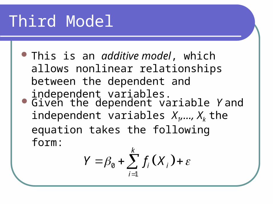
Third Model

This is an additive model, which allows nonlinear relationships between the dependent and independent variables.

Given the dependent variable Y and independent variables X1,…, Xk the equation takes the following form:

01

k

i ii

Y f X

Fourth Model

This adds a smooth function fitted to longitude and latitude to the additive model. This is called a geoadditive model in Kammann and Wand (2003).

Given the dependent variable Y, the independent variables X1,…, Xk, the longitude L1 and latitude L2 then the equation takes the following form:

0 1 21

,k

i ii

Y f X f L L

Smooth Functions

Univariate smooth functions were fitted using cubic smoothing splines.

Bivariate smooth functions were fitted using thin-plate smoothing splines, the natural bivariate extension of cubic smoothing splines.

Variable Selection

The same explanatory variables selected for the linear regression model were used for the other three functional forms.

This was to permit comparability of the four models and better understand the effects of including nonlinearity and spatial dependence on variable significance and magnitude

Variable Selection (cont.)

Factor analysis was used to separate the 45 variables into 8 categories.

Criteria for selecting variables were: parsimony, interpretability, significant effects, goodness of fit and meeting assumptions.

A modified form of forward selection was used – starting with several key variables such as distance from the city and lotsize

Results

Bivariate thin-plate splines could not be fit to the entire dataset, due to computational considerations

Linear regression and additive models were fit to the entire dataset

All four models were fitted to a random 1000 properties and the differences were analysed

Complete Dataset – Linear Regression

Variable Estimate Variable EstimateIntercept 13.07854 RailStatio

n0.00753

LotSize 0.00067 Park 0.00173

MainRoad

-0.03748 Highway 0.00172

NatPark -0.01256 Freeway 0.00813

Income 0.000459 Ambulance

-0.00257

PM10 -0.03728 AirNoise -0.00283

City -0.02547 Factory 0.00544

Complete Dataset – Additive model

Partial Plot for LotSize

Partial Plot for Income

Complete Dataset – Additive model (cont.)

Partial Plot for Air Pollution

Partial Plot for Distance to City

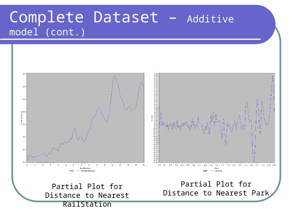
Complete Dataset – Additive model (cont.)

Partial Plot for Distance to Nearest RailStation

Partial Plot for Distance to Nearest Park

Complete Dataset – Additive model (cont.)

Partial Plot for Distance to Nearest Highway

Partial Plot for Distance to Nearest Freeway

Complete Dataset – Additive model (cont.)

Partial Plot for Aircraft Noise

Partial Plot for Distance to Nearest Ambulance Station

Complete Dataset – Additive model (cont.)

Partial Plot for Distance to Nearest Factory

Partial Plot for Distance to Nearest National Park

Complete Dataset – Additive model (cont.)

Partial Plot for Distance to Nearest Main Road

Partial Dataset Analysis

But the two fitted models do not account for spatial (auto)correlation

The effect of including bivariate smoothing into both models is analysed with the random 1000 properties discussed earlier

Comparison of linear models

Variable Lin. Reg. Lin. Reg. SS % Change

Intercept 13.14084 12.8749

Lotsize 0.00067 0.00066 -2.41

Income 0.00043 0.00023 -45.07

GPO -0.02724 -0.0288 5.73

PM10 -0.03691 Not significant

RailStation 0.01417 0.01471 3.81

Highway 0.02112 0.01676 -20.64

NatPark -0.0185 Not significant

Comparison of linear models (cont.)

The addition of bivariate smoothing is highly significant (p < 0.0001)

Magnitude and significance of variables is seen to be largely influenced by inclusion of this smoothing

Conclusion: spatial dependence is important and affects results

Comparison of additive models

Bivariate smoothing again highly significant

The addition of bivariate smoothing also changed which variables were significant in the additive model case

However for the 4 variables which are significant in the additive and geoadditive models, the effect is nearly unchanged.

Partial Plot for GPO in additive and geoadditive models

Partial Plot for Income in additive and geoadditive models

Partial Plot for LotSize in additive and geoadditive models

Partial Plot for RailStation in additive and geoadditive models

Conclusions

Additive models provide a more natural method of incorporating nonlinearities whilst maintaining the useful additive property

However further research is required in model selection and validation as well as analysis of spatial dependence and how it is best dealt with

Actuarial applications

(Generalised) additive models provide a significant extension of generalised linear models

Bivariate thin-plate splines are a new way to smooth spatial risk, which has been investigated by a number of papers, such as Fahrmeir et al. (2003)

Acknowledgements

Thanks to … The Environment Protection Authority

for financial assistance and dataTransport Data Centre also supplied

data under the Student Data programNRMA for use of mapping software

and expertiseResidex for property sale information