i

IMPACT OF MACROECONOMIC SHOCKS ON HOUSEHOLD POVERTY

AND INCOME INEQUALITY IN NIGERIA

BY

Nkang Moses NKANG

Matriculation Number: 131336

B.Agric., Agricultural Economics and Extension (Calabar)

M.Sc., Agricultural Economics (Calabar)

A THESIS IN

THE DEPARTMENT OF AGRICULTURAL ECONOMICS

SUBMITTED TO THE

FACULTY OF AGRICULTURE AND FORESTRY

IN PARTIAL FULFILMENT OF THE REQUIREMENTS FOR THE

DEGREE OF DOCTOR OF PHILOSOPHY OF

THE UNIVERSITY OF IBADAN

AUGUST, 2012

ii

ABSTRACT

Poverty and income inequality are huge development challenges in Nigeria. Over half

of the population are living below the poverty line, which is further accentuated by

highly skewed incomes. While it is widely held that the poor are more vulnerable to

economic shocks, empirical information regarding the degree to which these shocks

affect them is desired to ameliorate the problem. Hence, the impact of some

macroeconomic shocks on poverty and income inequality in Nigeria was investigated.

The National Living Standards Survey (NLSS) data of 2004 by the National

Bureau of Statistics and Nigeria‟s 2006 Social Accounting Matrix (SAM) by the

International Food Policy Research Institute (IFPRI) were used. The NLSS employed a

two-stage cluster sampling technique. The 19,158 housing units reported at the end of

the survey were used in the analysis. The NLSS provided data on households‟ income

and expenditure whereas the SAM provided data on production, income, consumption

and capital accumulation. The modified IFPRI SAM used comprised 21 matrix

accounts; made up of four activity sectors (food, other agriculture, crude oil and

manufacturing/services) and four different household groupings (rural-south, rural-

north, urban-south and urban-north). Data were analysed using Foster-Greer-Thorbecke

poverty measures and Gini-index, computable general equilibrium technique, and

sensitivity of poverty and inequality to macroeconomic shocks (fluctuations in food and

crude oil prices, exchange rate, and a combination of these).

Average incomes in rural-south and rural-north households were N234.0

(±206.8) and N211.5 (±198.2) per person per day respectively. Food and other

agricultural imports constituted 30.0% of total imports consumed by households.

Poverty incidence was 55.0%, 47.3%, 75.1%, 40.4% and 47.2% respectively for

Nigeria, rural-south, rural-north, urban-south and urban-north, while national inequality

was 0.42. A 50.0% rise in food price increased poverty by 4.9%, 2.0%, 3.9% and 4.2%

respectively for rural-south, rural-north, urban-south and urban-north. Conversely, a fall

in oil price by 50.0% increased poverty by 3.0% in rural-north but reduced same by

8.7%, 0.8% and 1.8% in urban-north, rural-south and urban-south respectively. A

25.0% depreciation in the exchange rate increased poverty by 2.5%, 0.3%, 2.2% and

3.3% respectively in rural-south, rural-north, urban-south and urban-north. The

combined impact of the shocks increased poverty by 8.6%, 7.1%, and 7.0% respectively

in rural-south, rural-north and urban-south, although shocks did not impact on poverty

among urban-north households. National inequality level dropped by 0.05% and 0.26%,

iii

respectively, following the increase in food price and exchange rate, while it rose by

1.41% due to the fall in oil price.

Overall, shocks impacted all household groups mostly negatively but rural-

north households were most affected, as they now accounted for about 47% of the poor

in Nigeria after the shocks. This indicates that the challenge of poverty reduction is

greatest in the rural-north, and hence interventions need be targeted at this region before

others.

Keywords: Macroeconomic shocks, Poverty incidence, Income inequality, Nigerian

households, Simulations

Word count: 457

iv

DEDICATION

To the two most important women in my life

My mother, Beatrice

For her selflessness

And

My love, Ann

For her inspiration

v

ACKNOWLEDGEMENTS

To Him, our Almighty God, who sits on the throne and unto the Lamb, our Lord Jesus

Christ, be all praise and honour, glory and power, forever; for most mercifully,

steadfastly and excellently seeing me through to the end of this pursuit of deepening

human knowledge for the benefit of mankind and the greater magnification of His holy

name!

I am indebted to my thesis committee for their effort to ensure that this research

work was well carried out. In particular, I am full of thanks for my major supervisor,

Dr. B. T. Omonona for his invaluable contributions toward my completion of this

programme: I am yet to meet any of his kind. I pray God Almighty, the provider of all

good things, to bountifully reward him for being an exemplification of godly virtues of

meekness, humility, sincerity and selflessness. My earnest appreciations go to Dr. S. A.

Yusuf for introducing me to general equilibrium modelling, and subsequently becoming

the „technical‟ supervisor of the thesis. His assistance and encouragement helped in no

small measure to bring this thesis to completion. He personally, facilitated my

attendance of a CGE workshop organized by the IFPRI in Abuja. That was actually my

first time in a CGE class! My thanks are also due to Dr. O. A. Oni, who even when he

became part of the thesis committee toward the end, contributed greatly, especially by

insisting on oral assessment rather than just written output. Last but by no means the

least in my gratitude to the committee, is my (posthumous) appreciation to late Dr.

(Mrs.) O. I. Y. Ajani, who was part of the supervision in the beginning but did not live

to see the completion of this work. May God Almighty grant her humble soul eternal

rest!

I thank my Head of Department, Professor V. O. Okoruwa, for his professional

advice, constructive criticism and facilitation of the process of completing this work. I

owe him a great depth of gratitude. I also wish to acknowledge the various contributions

of all other professors and lecturers in the department, especially the fatherly interest of

Professor A. O. Falusi, who was always concerned about knowing the progress of

everyone‟s research work, thus serving as a source of inspiration and support for us all.

I also am thankful to all other academic and administrative staff of the

Department of Agricultural Economics, University of Ibadan, particularly Mrs. Atanda,

Mrs. Oladejo, Mr. Lekan and Ms. Nike, for their support in the course of my studies at

the department.

vi

Professor A. Adenikinju and some lecturers in the Department of Economics

were most helpful at the beginning of this work and therefore deserve some credit. As

one of the pioneers of CGE modelling in Nigeria, apart from giving me technical

advice, Professor Adenikinju introduced me to the Economic Modelling (ECOMOD)

Network; he advised that if I wanted to have a practical grasp of the subject, then I

needed to attend one of their (ECOMOD) schools. That, I did, and the pay-off was quite

high! Dr. A. Aminu on his part helped to teach us the building blocks of CGE modelling

and also suggested some useful resources that helped me in the course of my research. I

also am thankful to Dr. O. Oyeranti for also being one of those from whose work I have

benefitted.

I would very much like to acknowledge the support of the University of Calabar;

for granting me Study Fellowship to pursue doctoral studies in the University of Ibadan

and for providing me with the initial funding for this programme. I thank the

International Food Policy Research Institute (IFPRI) in Abuja for selecting me as one of

the participants in the CGE modelling workshop in Abuja and more for providing the

Social Accounting Matrix that I used in the analysis.

My sincere appreciation goes to the Hewlett Foundation through the Institute for

International Education (IIE) for providing part of the funding for this research work

and for providing opportunities for networking with other researchers. I also am

thankful to the IIE, especially for making it possible for me to participate in the

2010/2011 Population Reference Bureau (PRB) Policy Fellows Programme. I am

indebted to my advisor at the PRB, Dr. Jay Gribble, for providing me with the tool-kit

for communicating research findings to policy audiences.

I am grateful to the ECOMOD Network, particularly to the instructors, Professor

Ali Bayar, Professor Can Erbil and Dr. Frederic Dramais, in the “Practical Techniques

in General Equilibrium Modelling with GAMS” class of the 2010 European School in

Istanbul. For without them, I may not have reached this stage just yet. I want to use this

opportunity to thank the PEP Network at the University of Laval, Canada for freely

providing the DAD software package which I used to implement part of the analyses in

this work.

To my colleagues in the postgraduate programme in the department, I say a big

thank you for your cooperation and support toward the completion of my research work.

I may not be able to acknowledge you all by name, but suffice it to say that you all were

wonderful, especially Mrs. Grace Evboumwan, Bola Awotide, Fatiregun Abosede,

vii

Olowe, Olowa, Bolaji, Ayobami and Ghene, and Mr. Busari Ahmed, Egbetokun,

Dontsop Nguezet, Waheed Ashar, John Odozie, Wale Olayide and Akuchi Nwigwe.

Some of my teachers and colleagues at the University of Calabar deserve special

mention. I would like to thank Dr. D. S. Udom for being a father and an academic

mentor to me: he instilled in me the spirit of academic discipline as far as research is

concerned, having supervised both my undergraduate project and master‟s thesis. I

thank Professors U. C. Amalu, S. B. A. Umoetuk and M. G. Solomon for their interest

in me and my doctoral studies, especially. I am grateful to Professor E. O. Eyo for his

understanding and support during his tenure as the head of the department of

Agricultural Economics and Extension, particularly after the expiration of my Study

Fellowship period. Drs. H. M. Ndifon, D. I. Agom, S. B. Ohen, E. A. Etuk, I. C. Idiong,

and A. O. Angba, and Mr. E. O. Edet were very supportive in various capacities as

colleagues and friends. I thank every other colleague whom I have not mentioned here

for the good and cordial relationship that we have enjoyed so far.

My friends and family have had to go on most of the time without me in the

course of this work. Sometimes I have had to be absent in many important occasions at

home, and in social and community functions, which I needed to be part. To all who in

one way or the other represented or had to protect my interest in all such occasions, I

owe a depth of gratitude. Noteworthy is the unflinching and unalloyed support of my

honorary son, Columbanus Mbey Ntui. His dedication, loyalty and exemplary

followership deserve commendation and have made him one among equals. I thank him

sincerely for being a good son.

I thank my parents, Mr. and Mrs. M. T. Nkang for their prayers, understanding

and trust in me, even when it took so long to get here. I pray God to give them many

more years to live and reap from the fruit of the labour of their hands. And to all my

brothers and sisters, I thank you all for standing by me and providing support when it

was needed in the course of this endeavour. I am also appreciative of the moral support

of my parents-in-law, Sir and Mrs. J. W. Nku, especially Sir Nku for his interest in my

academic pursuit. My sister-in-law and cousin-in-law, Kyije and Ada were most useful

at the domestic front.

I lack words to express my thanks to my greatest motivator and critic, my wife

and love, Ann. She has been exceedingly supportive. I thank you especially for

believing in me and standing by me even when it got really tough. To our Cherry,

viii

Khloe, thank you for being a happy child and source of joy; I am exceedingly grateful to

God for giving you to us.

Finally, I owe a lot of (posthumous) gratitude to my late friend, Dr. S. E. Ibana,

for encouraging me to pursue my doctoral degree in the University of Ibadan. Without

him, I do not think that I would have been exposed to all that has come my way in the

course of my PhD studies. May his gentle soul rest in peace!

Nkang Moses Nkang

ix

CERTIFICATION

I certify that this work was carried out by Mr. Nkang Moses NKANG in partial

fulfilment of the requirements for the award of the degree of Doctor of Philosophy in

Agricultural Economics, under my supervision.

Supervisor

B. T. Omonona

B.Sc., M.Sc., PhD (Ibadan)

Senior Lecturer in Welfare Economics and Quantitative Analysis

Department of Agricultural Economics

University of Ibadan, Ibadan, Nigeria

x

TABLE OF CONTENTS

Title Page i

Abstract ii

Dedication iv

Acknowledgements v

Certification ix

Table of contents x

List of Tables xiv

List of Figures xv

CHAPTER ONE: INTRODUCTION

1.1 Background to the Study 1

1.2 Poverty and Inequality Trends in Nigeria 6

1.3 Poverty Alleviation Initiatives in Nigeria 11

1.4 Problem Statement 14

1.5 Objectives of the Study 16

1.6 Justification of the Study 16

1.7 Organisation of Study 18

CHAPTER TWO: CONCEPTUAL FRAMEWORK AND THEORETICAL

LITERATURE REVIEW

2.1 Introduction 19

2.2 Concept of Shock 19

2.2.1 Economic Shocks 20

2.2.2 Macroeconomic Shocks 21

2.2.3 Types of Economic Shocks 21

2.2.3.1 Demand Shocks 22

2.2.3.2 Supply Shocks 23

2.3 Concept of Poverty 24

2.3.1 Measurement of Poverty 28

2.3.1.1 Why Measure Poverty? 28

2.3.1.2 Properties of a Good Poverty Measure 31

2.3.1.3 Absolute Poverty 31

2.3.1.4 Relative Poverty 32

2.3.2 Causes of Poverty 33

xi

2.4 Concept of Inequality 36

2.4.1 Measurement of Inequality 37

2.4.1.1 Why Measure Inequality? 38

2.4.2 Poverty versus Inequality: The Nexus 39

2.5 Macroeconomic Shocks, Poverty and Inequality: The Transmission

Channels 42

2.5.1 Prices (Production, Consumption and Wages) 44

2.5.2 Employment and Incomes 44

2.5.3 Government Expenditures 45

2.5.4 Assets 45

2.5.5 Access to Goods and Services 46

2.6 Transmission Mechanisms of Shocks Studied 46

2.6.1 Food Price Shock 46

2.6.2 Oil Price Shock 47

2.6.3 Exchange Rate Shock 47

2.7 Methodological/Analytical Concepts 48

2.7.1 General Equilibrium Theory 49

2.7.2 Computable General Equilibrium Analysis 50

2.7.2.1 Representative Household (RH) CGE Model 53

2.7.2.2 Integrated Multi-Household (IMH) CGE Model 53

2.7.2.3 Micro-simulation (MS) CGE Model 54

CHAPTER THREE: REVIEW OF RELATED EMPIRICAL LITERATURE

3.1 Introduction 55

3.2 Nigeria-based Studies 55

3.3 Other Studies 61

3.4 Summary 69

CHAPTER FOUR: METHODOLOGY

4.1 Introduction 70

4.2 Data and Sources of Collection 70

4.2.1 Description of the Social accounting Matrix 70

4.2.2 Nigeria Living Standards Survey Data 72

4.3 Analytical Framework 72

4.3.1 Model Specification 74

xii

4.3.1.1 Specification and Description of the CGE Model for the Study 74

4.3.1.1.1 Definitions of Parameters and Variables in the CGE Model 75

4.3.1.1.2 Equations in the CGE Model for Nigeria 78

4.3.1.1.3 Calibration of the CGE Model 84

4.3.1.2 Poverty Analysis and inequality Analyses in the Study 86

4.3.1.2.1 Poverty Analysis 86

4.3.1.2.2 Inequality Analysis 88

4.3.2 Model Implementation Procedures 89

4.3.2.1 CGE Analysis (GAMS) 89

4.3.2.2 Poverty and Inequality Analysis (DAD) 91

4.3.3 Description of and Rationale for Model Simulation Experiments 91

CHAPTER FIVE: RESULTS AND DISCUSSION

5.1 Introduction 93

5.2 Descriptive Analysis of the Structure of the Economy in the Base Year 93

5.2.1 Sources of Household Income 93

5.2.2 Uses of Household Income 95

5.2.3 Sectoral Factor Remunerations and Factor Market Shares 96

5.2.4 Household Consumption and Import Intensity 97

5.2.5 Government Revenue and Expenditure 97

5.3 Base Equilibrium Solution of the CGE Model 98

5.4 Simulation Results 100

5.4.1 Rise in World Price of Food Imports 101

5.4.2 Fall in World Price of Oil Exports 102

5.4.3 Depreciation of the Exchange Rate 104

5.4.4 Combination of the Three Scenarios 106

5.5 Poverty Status of Households in the Base Year 107

5.6 Impact of Simulations on Poverty 110

5.6.1 Impact of Food Price Shocks on Poverty 110

5.6.2 Impact of Oil Price shocks on Poverty 112

5.6.3 Impact of Exchange Rate shocks on Poverty 114

5.6.4 Impact of All shocks Combined on Poverty 116

5.6.5 Comparison of the Impacts of Simulations on Household Groups

by Poverty Gap Measure and Equally Distributed Equivalent Income 118

xiii

5.7 Impact of Simulations on Income Inequality 119

CHAPTER SIX: SUMMARY, CONCLUSIONS AND RECOMMENDATIONS

6.1 Introduction 122

6.2 Summary of Major Findings 122

6.3 Conclusions 125

6.4 Policy Recommendations 126

6.5 Limitations of the Study and Suggestions for Further Research 129

References 131

Appendix I

Appendix II

xiv

LIST OF TABLES

Table 1.1: Poverty Headcount in Nigeria, 1980 – 2004 8

Table 1.2: Moderately Poor and Core Poor in Nigeria, 1980 – 2004 9

Table 1.3: Incidence of Poverty by Sector and Zones in Nigeria, 1980-2004 9

Table 1.4: Poverty Incidence by Educational Levels of Household

Heads in Nigeria, 1980 – 2004 10

Table 1.5: Poverty Incidence by Occupation of Household Heads in Nigeria,

1980 – 2004 10

Table 1.6: Inequality Trend by Sector and Zones in Nigeria, 1985 -2004 11

Table 4.1: Aggregation of Sectors in the Original into Sectors in the New

SAM 71

Table 5.1: Sources of Household Income 94

Table 5.2: Uses of Household Income 95

Table 5.3: Sectoral Factor Remunerations and Factor Market Shares 96

Table 5.4: Household Consumption Shares and Import Intensity 97

Table 5.5: Government Revenues 98

Table 5.6: Government Expenditure 98

Table 5.7: Replicated Benchmark Data 99

Table 5.8: Simulation Results of Food Price Shocks 101

Table 5.9: Simulation Results of Oil Price Shocks 103

Table 5.10: Simulation Results of Exchange Rate Shocks 105

Table 5.11: Simulation of Combination of Three Scenarios 106

Table 5.12: Poverty Status of Households in the Base Year 108

Table 5.13: Impact of Food Price Shock on Poverty (Percent) 111

Table 5.14: Impact of Oil Price Shock on Poverty (Percent) 113

Table 5.15: Impact of Exchange Rate Shock on Poverty (Percent) 115

Table 5.16: Impact of All Shocks Combined on Poverty (Percent) 117

Table 5.17 Impacts on Poverty Gap and Equally Distributed

Equivalent Income 119

Table 5.18: Inequality Levels in the Base Year 120

Table 5.19: Impact of Simulation on Base Inequality Levels (Percent) 121

xv

LIST OF FIGURES

Figure 1.1: Annual Food Price Indices of Selected Food Commodities,

1998 – 2009 (2002-2004=100) 3

Figure 1.2: Average Monthly Crude Oil Prices, 2007 – 2009 5

Figure 1.3: Average Monthly Exchange Rate (N/USD 1.00)

August 2008 – July 2009 6

Figure 2.1: Impact of a Demand Shock in the Economy 23

Figure 2.2: Impact of a Supply Shock in the Economy 24

Figure 2.3: Poverty-Growth-Inequality Triangle 40

Figure 5.1 Poverty Status of households in the Base Year 109

Figure 5.2 Impact of Food Price Shock on Poverty 112

Figure 5.3 Impact of Oil Price Shock on Poverty 114

Figure 5.4 Impact of Exchange Rate Shock on Poverty 116

Figure 5.5 Impact of the Combined Shock on Poverty 118

Figure 5.6 Equally Distributed Equivalent Income by Household

Groups Following the Shocks 119

1

CHAPTER ONE

INTRODUCTION

No Society can surely be flourishing and happy, of which the far greater part of the

members are poor and miserable.

- Adam Smith

1.1 Background to the Study

Economic crises have often been accompanied by shocks which may be

idiosyncratic or covariate (macroeconomic) in nature. Existing empirical evidence

suggests that macroeconomic shocks can cause social distress, which manifests directly

or indirectly in increased poverty and inequality levels among other welfare issues, as a

result of a fall in output and real incomes associated with a crisis (Lustig, 1998 and

2000; Skoufias, 2003; Damuri & Perdana, 2003; Essama-Nssah, 2005; Conforti and

Sarris, 2009).

Further evidence reported by Lustig (2000), Mbabazi (2002), Skoufias (2003),

World Bank (2008), among others, has shown that developing countries are mostly

affected by the impact of macroeconomic shocks following an economic crisis. In

particular, according to the World Bank (2008) an additional 20 million people on

average are pushed into poverty, as a result of a one percent fall in the growth of output

of developing countries following a crisis. This, they however stated depends, amongst

other factors, on the distribution of income, social policies, and the sector/geographic

incidence of changes in income.

Poverty and inequality have been found to be implicitly related apart from their

indirect relationship via economic growth (Bourguignon, 2004; Aigbokhan, 2008).

Given this relationship, it has been recognised by Hanmer and Naschold (2000), that at

least in the context of Africa, the Millennium Development Goals (MDGs) on poverty

reduction cannot be achieved without reductions in inequality, as it has been

documented that income inequality matters when it comes to making progress on

poverty reduction (Addison and Cornia, 2001; Naschold, 2002). Thus, as a developing

country and one that has had a historical record of high levels of poverty and inequality,

the recent world economic crisis would have impacted Nigeria‘s economy in several

ways and in varying degrees.

The economic crisis, which started with the steep rise in world food prices

between mid-2007 and mid-2008, was a cause of grave concern among policymakers as

it portended huge implications for poverty and food insecurity in low income countries

2

(Ellis and White, 2010). The food price crisis was linked to poor harvests in Australia

and Russia, increase in bio-fuel production, diminished world food stocks, export bans

in leading exporting countries, among other factors. World Bank researchers had

predicted that rising commodity prices would cause the poverty headcount in low

income countries to increase by more than 100 million (Ivanic and Martin, 2008),

including over 30 million in Africa alone (Wodon and Zaman, 2008).

Worsening the food price crisis was a quick upward jump in oil prices, which

was attributed on one hand to rapid economic growth, particularly in India and China,

and on the other, to speculative behaviour around future long-run scarcity. Indeed, the

price of oil hit an historic high of US$140 per barrel in June 2008. For a net oil

exporting country like Nigeria, this was a signal of good fortunes, but it turned out to be

very short-lived.

From June 2008, all prices began to decline, although at various rates. The

decline in cereal prices was initially linked to good harvests arising from favourable

weather conditions and the incentive provided by the initial high prices which had

boosted planted area. However, the major reason for this rapid decline was the emerging

global financial crisis which was triggered by global banking crisis caused by the over-

exposure of banks in the US and Europe to financial derivatives based in non-

performing loans. By September 2008 a meltdown of the international financial system

was in sight, prompting one of the most dramatic reversals in oil prices, which in turn

fed into the cereal price fall. Thus, the financial crisis was seen as adding to the severity

of the circumstances facing the poorest countries, and the discussion turned to the so-

called ‗3 Fs crisis‘ for food, fuel, and finance (Ellis and White, 2010).

During the crisis, the Nigerian economy experienced a flurry of exogenous

shocks, which could portend far-reaching macroeconomic impacts, especially on the

wellbeing of households which are a core entity in development and poverty reduction

endeavours. Prominent among these shocks were increased domestic and imported food

prices, a fall in oil revenues, following the sudden plunge in oil prices in the

international market, and depreciation of the real exchange rate, among others (see,

Soludo, 2009).

The food price shocks experienced during the crisis, and attributed to increasing

global demand for food, high fuel prices and adverse supply movements could portend

diverse implications for the poor, especially the impact on their real incomes. Agenor

(2005) notes that because the poor allocate a large share of their income (or own

3

production, if they are self-employed in agriculture or the urban informal sector) to

subsistence, the impact of macroeconomic price shocks on the goods and services that

they consume matters significantly. Indeed, it is widely accepted that high food prices

were having a more adverse impact on the poor because of the disproportionately high

amount that is spent on food, since they pay more for their food and receive less for

their produce (FAO, 2009). World food prices had risen by 53 percent during the crisis,

based on the FAO food price index for the first three months of 2008, (Reyes,

Sobrevinas, Bancolita and de Jesus, 2008; FAO, 2009), thus leading to increased social

tensions and political upheavals in net food importing countries, and food export

restrictions in net exporting countries. The extent of this shock, based on FAO statistics,

is depicted in Figure 1.1 below.

Source: Boccanfuso and Savard, 2009

Figure 1.1: Annual food price indices of selected food commodities, 1998 – 2009

(2002-2004=100)

The intervention in the food price crisis in Nigeria in 2009 by the Federal Government

underscores the explosive nature of food prices during the crisis. To ameliorate the

impact of this shock, government had announced the removal of import tariff on rice,

the single most important staple food import in Nigeria, for six months, in order to

mitigate the adverse impact of increased prices on consumers. The intervention by

government was not only a temporary measure of mitigating the social cost of adverse

price shocks, but was also hardly, informed by facts regarding the segments of the

4

economy that needed the most help. Thus, the need for an empirical investigation of the

impacts of the food price shocks on socioeconomic groups, merits consideration.

Away from the food price shocks, the plunge in oil prices was also a cause for

concern for a net oil exporting country like Nigeria. The effect of extreme volatility,

especially, falling crude oil prices can be better appreciated from the point of view of its

importance in fiscal (budget) policy. Crude oil exports play a significant role in the

Nigerian economy as evidenced not only in being the largest contributor in terms of

total government revenue but also as the overall leader in her exports composition.

Approximately 95 percent of Nigeria‘s exports come from oil and this, according to the

World Bank (2003), has not changed much since 1974. More recent data show that

crude oil contributes over 90 percent to total exports and roughly 30 percent to Gross

Domestic Product (GDP), aside constituting about 80 percent of government revenues

(CBN, 2006; Akpan, 2009; Kilishi, 2010, among others). Consequently, a small change

in oil price, be it a rise or fall, can have a large impact on the economy. For example,

Kilishi (2010), notes that a US$1 increase in oil price in the early 1990s increased

Nigeria‘s foreign exchange earnings by about US$650 million (2 percent of GDP) and

its public revenues by US$320 a year.

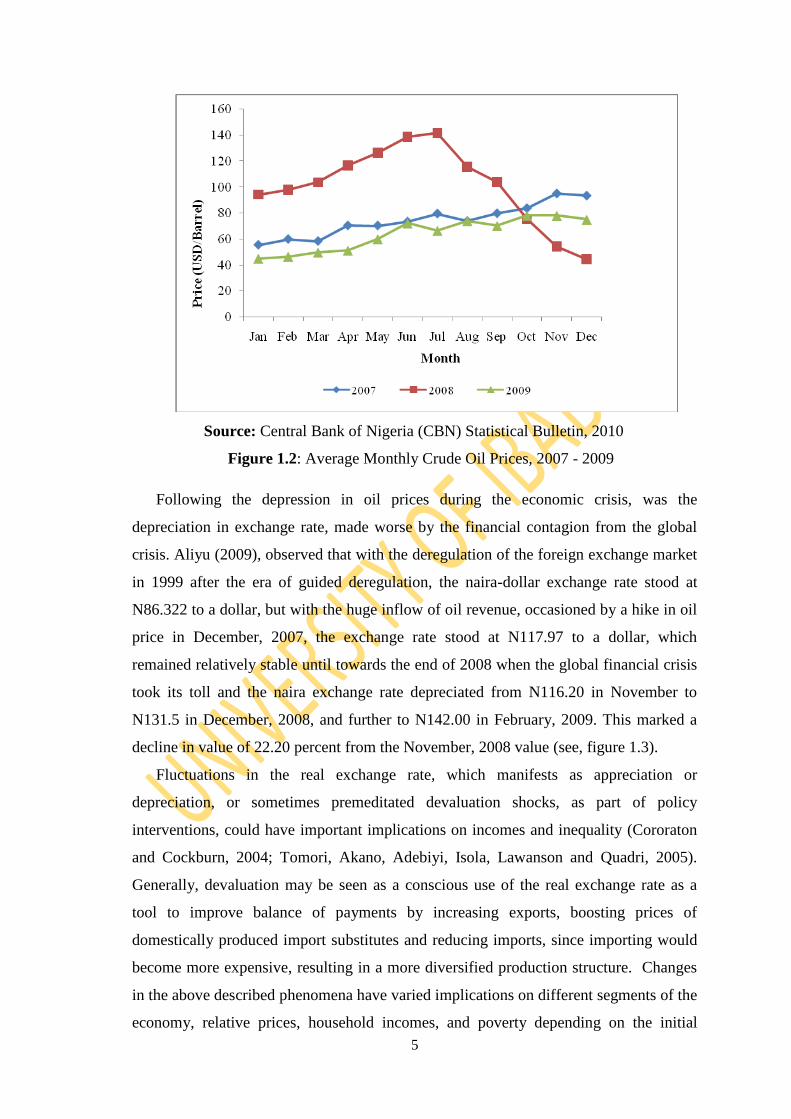
In 2008, oil prices rose to an all time high of over US$140 per barrel in July/August

(see, figure 1.2) and dropped abruptly to less than US$40 per barrel by December, when

the 2009 appropriation bill was presented to the National Assembly. This indicates a

decline of about 250 percent at the time, thus fuelling concerns about its impacts on the

economy and the wellbeing of citizens. The explosive nature of oil prices in the world

market makes the Nigerian economy vulnerable to this external shock despite being the

6th

largest producer of crude oil in the world, and has caused among other problems,

instability in government fiscal revenues as well as terms of trade shocks owing to the

country‘s high dependence on oil. Given that fiscal revenue volatility is frequently cited

as a source of difficulty in delivering high quality public services that reduce poverty,

then investigating the effect of this shock in the context of the recent crisis becomes

very vital.

5

Source: Central Bank of Nigeria (CBN) Statistical Bulletin, 2010

Figure 1.2: Average Monthly Crude Oil Prices, 2007 - 2009

Following the depression in oil prices during the economic crisis, was the

depreciation in exchange rate, made worse by the financial contagion from the global

crisis. Aliyu (2009), observed that with the deregulation of the foreign exchange market

in 1999 after the era of guided deregulation, the naira-dollar exchange rate stood at

N86.322 to a dollar, but with the huge inflow of oil revenue, occasioned by a hike in oil

price in December, 2007, the exchange rate stood at N117.97 to a dollar, which

remained relatively stable until towards the end of 2008 when the global financial crisis

took its toll and the naira exchange rate depreciated from N116.20 in November to

N131.5 in December, 2008, and further to N142.00 in February, 2009. This marked a

decline in value of 22.20 percent from the November, 2008 value (see, figure 1.3).

Fluctuations in the real exchange rate, which manifests as appreciation or

depreciation, or sometimes premeditated devaluation shocks, as part of policy

interventions, could have important implications on incomes and inequality (Cororaton

and Cockburn, 2004; Tomori, Akano, Adebiyi, Isola, Lawanson and Quadri, 2005).

Generally, devaluation may be seen as a conscious use of the real exchange rate as a

tool to improve balance of payments by increasing exports, boosting prices of

domestically produced import substitutes and reducing imports, since importing would

become more expensive, resulting in a more diversified production structure. Changes

in the above described phenomena have varied implications on different segments of the

economy, relative prices, household incomes, and poverty depending on the initial

6

economic structure, available incentives, safety-net programmes and level of social

protection and or policy responses.

Source: Central Bank of Nigeria (CBN) Statistical Bulletin, 2010

Figure 1.3: Average Monthly Exchange Rate (N/USD 1.00) August 2008 – July 2009

Literature has shown that the impacts of the outline shocks are economy-wide in

nature, having direct and indirect as well as micro and macro repercussions in the

economy and on poverty and income distribution (Lustig and Walton, 1998; Ferreira,

Prennushi and Ravallion, 1999; Winters, 2000; Cockburn, Decaluwe and Robichaud,

2008; Mendoza, 2009). In view of their economy-wide nature, these shocks are better

studied in a general equilibrium framework in other to capture the interrelationships

among all sectors and agents in the economy. Consequently, this study is an attempt to

quantitatively trace the impacts of the previously highlighted negative macroeconomic

shocks on Nigerian households in terms of poverty and inequality, using general

equilibrium techniques with a view to providing empirical evidence to guide policy

intervention and stimulate further inquiry in this area of study.

1.2 Poverty and Inequality Trends in Nigeria

According to the NBS (2005), Nigeria emerged from colonial status as a poor

country. This situation has not changed much until now. Instead, poverty in Nigeria has

worsened and remained widespread and persistent. Be that as it may, in Nigeria, poverty

is largely a rural phenomenon, as the economy is characterized by a large rural, mostly

agriculture-based, traditional sector, which is home to about three-fourths of the poor,

7

and by a smaller urban capital intensive sector, which has benefited most from the

exploitation of the country‘s resources and from the provision of services that

successive governments have provided (Omonona, 2001 & 2009; Yusuf, 2002; NBS,

2005; Obi, 2007, among many). In spite of the benefits enjoyed by the urban sector,

poverty still exists in urban areas substantially thus mirroring the endemic nature of the

problem.

Thus, according to Obi (2007), the poor in Nigeria are not a homogeneous

group. They can be found among several social/occupational groups and can be

distinguished by the nature of their poverty. Using 1992/93 household survey data, the

World Bank poverty assessment on Nigeria showed that the nature of those in poverty

can be distinguished by several characteristics, which include sector, education, age,

gender and employment status of the head of household (FOS,1995). Other

characteristics included household size and the share of food in total expenditure.

Several causes have been advanced for the precarious poverty and inequality

situation in Nigeria. They include, but may not be limited to, inadequate access to

employment opportunities for the poor, lack or inadequate access to assets such as land

and capital by the poor; inadequate access to the means of fostering rural development

in poor regions; inadequate access to markets for the goods and services that the poor

produce; inadequate access to education, health, sanitation and water services; the

destruction of the natural resource endowments, which has led to reduced productivity

of agriculture, forestry and fisheries; the inadequate access to assistance by those who

are the victims of transitory poverty such as droughts, floods, pests and civil

disturbances and inadequate involvement of the poor in the design of development

programmes. These multidimensional causes of material and non-material deprivation

make poverty to be very endemic in Nigeria (FOS, 1996).

However, the worsening of poverty in Nigeria, according to UNSN (2001) can

be traced to factors such as poor and inconsistent macroeconomic policies, weak

diversification of the economic base, gross economic mismanagement, weak inter-

sectoral linkages, and persistence of structural bottlenecks in the economy, high import

dependence and heavy reliance on crude oil exports. Other factors include the long

absence of democracy and the usurpation of political power by the military elite, lack of

transparency and high level of corruption, declining productivity and low morale in the

public service, as well as ineffective implementation of relevant policies and

programmes (Tomori et al, 2005).

8

The National Bureau of Statistics (NBS), formerly Federal Office of Statistics

(FOS) has conducted several nationally representative household surveys (1980,

1985/86, 1992/93 and 2003/2004) with a view of providing a poverty profile for

Nigeria, among other considerations. Based on these surveys, a summary of the poverty

and inequality statistics in Nigeria is presented in the tables that follow (see also

Aigbokhan, 2008). NBS (2005) reports that the relative poverty measure used was

based on one-third and two-third of mean per capita expenditure for core poor and

moderately poor, respectively.

The statistics for poverty incidence and estimated population poverty shown in Table

1.1 revealed that poverty headcount dropped from 46.3 percent in 1985 to 42.7 percent

in 1992; it rose sharply to 65.6 percent of the population in 1996 and then declined

moderately to 54.4 percent in 2004. Nonetheless, in terms of absolute number of people

living in poverty, the population of the poor in Nigeria increased almost four-fold

between 1980 and 2004.

Table 1.1: Poverty Headcount in Nigeria, 1980 - 2004

Year Poverty

Incidence (%)

Estimated Population

(Millions)

Population in Poverty

(Millions)

1980 28.1 65 17.7

1985 46.3 75 34.7

1992 42.7 91.5 39.2

1996 65.6 102.3 67.1

2004 54.4 126.3 68.70

Source: National Bureau of Statistics (NBS, 2005)

Statistics showing the proportion of the non-poor, moderately-poor and core-

poor shown in Table 1.2 reveal that the core-poor still make up about 40 percent of the

poor in Nigeria as at 2004. Of particular note is that the proportion of the core-poor was

more than doubled between 1992 and 1996 compared with that of the moderately-poor

which increased only slightly.

9

Table 1.2: Poor and Core Poor in Nigeria, 1980 - 2004

Year Non Poor (%) Mod. Poor (%) Core Poor (%)

1980 72.8 21.0 6.2

1985 53.7 34.2 12.1

1992 57.3 28.9 13.9

1996 34.4 36.3 29.3

2004 45.6 32.4 22.0

Source: National Bureau of Statistics (NBS), 2005

The statistics in Table 1.3 further shed light on the nature of poverty in Nigeria.

It can be observed that urban poverty rose from 17.2 percent in 1980 to 58.2 percent in

1996, and by 2004 it declined substantially to 43.2 percent. In the same vein, there was

a rise in rural poverty from 28.3 percent in 1980 to 69.3 percent in 1996, but dropped

marginally to 63.3percent in 2004, suggesting a more precarious situation in rural areas.

Furthermore, when disaggregated by zones, it was clear that poverty is more

concentrated in the northern zones compared with the southern zones. For example, in

2004, over 70 percent of those living in the north-east and north-western zones were

poor.

Table 1.3: Incidence of Poverty by Sector and Zones in Nigeria, 1980-2004

1980 1985 1992 1996 2004

National 28.1 46.3 42.7 65.6 54.4

Sector

Urban 17.2 37.8 37.5 58.2 43.2

Rural 28.3 51.4 66.0 69.3 63.3

Geo-Political Zone

South South 13.2 45.7 40.8 58.2 35.1

South East 12.9 30.4 41.0 53.5 26.7

South West 13.4 38.6 43.1 60.9 43.0

North Central 32.2 50.8 46.0 64.7 67.0

North East 35.6 54.9 54.0 70.1 72.2

North West 37.7 52.1 36.5 77.2 71.2

Source: NBS, 2005 and Aigbokhan, 2008

Looking more into the challenge of poverty in Nigeria, we consider the

educational dimension of poverty as depicted in Table 1.4. First, it can be observed that

poverty incidence decreases as one moves from no schooling to post secondary

schooling, except for 1980, indicating that heads of household with no education are

most likely to be in poverty. Second, the table reveals that between 1980 and 2004,

poverty incidence increased over two-fold for all educational groups and all Nigeria.

10

Table 1.4: Poverty Incidence by Educational Levels of Household Heads in

Nigeria,

1980-2004

1980 1985 1992 1996 2004

No schooling 30.2 51.3 46.4 72.6 68.7

Primary 21.3 40.6 43.3 54.4 48.7

Secondary 7.6 27.2 30.3 52.0 44.3

Post

secondary

24.3 24.2 25.8 49.2 26.3

All Nigeria 27.2 46.3 42.7 65.6 54.4

Source: FOS (1999) Poverty Profile for Nigeria 1980 – 96, and NBS (2005) Poverty

Profile for Nigeria, Abuja

The occupational dimension of poverty incidence is pictured in Table 1.5.

Generally, households whose heads engaged in agriculture had the highest incidence of

poverty, except in 1980 and 1996. This was followed by households whose heads were

engaged in the transport and production sector. About 67 percent of those in agricultural

occupation in 2004 were poor compared with 31.5 percent in 1980. The highest poverty

levels across almost all the occupations were experienced in 1996. This was probably

due the abandonment of the rural agricultural policies implemented between 1986 and

1992 as part of the Structural Adjustment Programme (SAP). In all, the occupational

perspective of poverty in Nigeria further affirms the endemic nature of the problem.

Table 1.5: Poverty Incidence by Occupation of Household Heads in Nigeria, 1980 -

2004

1980 1985 1992 1996 2004

Professional & Technical 17.3 35.6 35.7 51.8 34.2

Administration 45.0 25.3 22.3 33.5 45.3

Clerical & related 10.0 29.1 34.4 60.1 39.2

Sales Workers 15.0 36.6 33.5 56.7 44.2

Service Industry 21.3 38.0 38.2 71.4 43.0

Agricultural & Forestry 31.5 53.5 47.9 71.0 67.0

Production & Transport 23.2 46.6 40.8 65.8 42.5

Manufacturing & Processing 12.4 31.7 33.2 49.4 44.2

Others 1.5 36.8 42.8 61.2 49.1

Student & Apprentices 15.6 40.5 41.8 52.4 41.6

Total 27.2 46.3 42.7 65.6 54.4

Source: NCS 1980, 1985, 1992, 1996, 2004

Since inequality as a measure of wellbeing matters for poverty, any meaningful

discussion of poverty indices should consider inequality indices too. Inequality is

important for poverty because according to McKay (2002), for a given level of average

11

income, education, land ownership, etc, increased inequality of these characteristics will

almost always imply higher levels of both absolute and relative deprivation in these

dimensions. Based on this reasoning, it is expected that efforts to bridge inequality gaps

would most likely result in poverty reduction. Table 1.6 shows inequality trends by

sector and zones in Nigeria as measured using the Gini coefficient.

Estimates in the table clearly indicate that at the national level, there was a rise

in inequality from 1985 to 2004, although a slight decline was witnessed in 1992. At the

sectoral and regional levels, there are some noticeable deviations from the national

average inequality for the years under consideration. Furthermore, inequality increased

markedly between 1996 and 2004. Aigbokhan (2008) contends that the national average

inequality may have concealed rising inequality across states and sectors since the mid-

1990s.

The statistics underlying the poverty and inequality situation in Nigeria

seem incongruous in the face of the perceived abundant national wealth and the various

programmes and policies that have been geared at poverty reduction in almost the last

three decades. In next subsection we shall briefly discuss some key the poverty

alleviation initiatives in Nigeria.

Table 1.6: Inequality Trend by Sector and zones in Nigeria, 1985 -2004

1985 1992 1996 2004

National 0.43 0.41 0.49 0.488

Sector

Urban 0.49 0.38 0.52 0.544

Rural 0.36 0.42 0.47 0.519

Geo-Political Zone

South South 0.48 0.39 0.46 0.507

South East 0.44 0.40 0.39 0.449

South West 0.43 0.40 0.47 0.554

North Central 0.42 0.39 0.50 0.393

North East 0.39 0.40 0.49 0.469

North West 0.41 0.43 0.47 0.371

Source: Aighbokhan, 2008

1.3 Poverty Alleviation Initiatives in Nigeria

Following NBS (2005), past government efforts in poverty alleviation can be

categorized into three main eras. These include those pursued before the Structural

Adjustment Programme (SAP), during the Structural Adjustment Programme era/the

Abacha regime and those initiated during the return to civil rule from 1999 to present.

12

Prior to the SAP era, poverty reduction programmes emphasized increased

production and supply of food on the premise that availability of cheap food will mean

higher nutrition levels and invariably lead to national growth and development. The

programmes were also aimed at the provision of basic social and economic

infrastructure that would boost employment generation, increase productivity, enhance

incomes, and lead to a more egalitarian distribution of incomes. Notable among these

programmes were the Operation Feed the Nation, OFN (1979) of the Military regime of

Obasanjo and the Green Revolution (1979-1983) of the Shagari‘s administration.

The military regime of Buhari (1983-1985) did not have a specific poverty

alleviation programme, as it clearly focused on fighting indiscipline and corruption,

through the War Against Indiscipline, WAI, initiative, which, according to some

analysts was equal to a poverty alleviation programme in the sense that indiscipline and

corruption were partly the reason why many Nigerians were poor (Anonymous, 2011).

The Structural Adjustment Programme, SAP era, which spanned almost the

entire Babangida administration (1985 – 1993), witnessed a broad range of poverty

alleviation projects/programmes. The SAP stressed greater realization of the need for

policies and programmes to alleviate poverty and provide safety-nets for the poor.

Government efforts then could be categorized into nine groups: These were Agricultural

Sector Programmes; Health Sector Programmes; Nutrition-related Programme;

Education Sector Programmes; Transport Sector Programmes; Housing Sector

Programmes; Financial Sector Programmes; Manufacturing Sector Programmes and

Cross-Cutting Programmes. To implement some of these programmes, some institutions

and agencies were established. These included People‘s Bank, Community Banks,

Directorate of Food, Roads and Rural Infrastructure (DFRRI), Nigerian Agricultural

Land development Authority (NALDA), National Directorate of employment (NDE)

and Better Life for Rural Women.

According to analysts, the SAP failed because it had no human face in its

implementation and it did not emphasize on human development which thereby

aggravated socio-economic problems of income inequality, unequal access to food,

shelter, education, health and other necessities of life. It ended up aggravating poverty

especially among the vulnerable.

The Abacha regime introduced the Family Economic Advancement Programme

(FEAP) out of the pursuit for a way out of unbearable poverty, occasioned by the

ranking of Nigeria as one of the 25 poorest nations in the world. FEAP existed for about

13

two years (1998 – 2000) during which it received funding to the tune of N7 billion out

of which about N3.3 billion was disbursed as loans to about 21,000 cooperative

societies nationwide that were production oriented. There was also the Family Support

Programme (FSP) which was basically targeted at women during the Abacha regime.

The FSP introduced a gender element into anti-poverty programmes, based on the

assumption that women needed special treatment because of their immense

contributions to the national economy, both as small-scale entrepreneurs and home

keepers.

However, based on a recent government assessment, most of these poverty

alleviation programmes failed due largely to the fact that they not only lacked a clearly

defined policy framework with proper guidelines for poverty alleviation but also lacked

continuity as they suffered from policy instability, political interference, policy and

macroeconomic dislocations, among other problems (Obadan, 2002).

Consequent upon the experiences of the past, the Obasanjo civilian

administration which had at inception in May 1999 set out poverty reduction as one of

its areas of focus, approved the blueprint for the establishment of the National Poverty

Eradication Programme (NAPEP) – a central coordination point for all anti-poverty

efforts from the local government level to the national level by which schemes would be

executed with the sole purpose of eradicating absolute poverty. Some of such schemes

identified include: Youth Empowerment Scheme (YES), Rural Infrastructures

Development Scheme (RIDS), Social Welfare Services Scheme (SOWESS) and Natural

Resource Development and Conservation Scheme (NRDCS) (see, Aliu, 2001). With a

take-off grant of N6 billion approved for it in 2001, NAPEP has established structures at

all levels nationwide. Under its Capacity Acquisition Programme (CAP), it trained

100,000 unemployed youths just as 5,000 others who received training as tailors and

fashion designers, were resettled. A total of 50,000 unemployed graduates have also

benefited from NAPEP‘s Mandatory Attachment Programme, which is also an aspect of

CAP. The World Bank (2001/2002) later had to assist Nigeria in formulating poverty

strategy programmes and policies through Interim Poverty Reduction Strategy Paper

(IPRSP) with the aim of building on the gains of the earlier efforts on poverty

programmes (PAP and PEP).

In the face of the growing concern to sustain the gains of the poverty efforts, the

administration came up with a comprehensive home-grown poverty reduction strategy

known as National Economic Empowerment and Development Strategy (NEEDS) in

14

2004. The NEEDS also builds on the earlier two years‘ efforts to produce the interim

PRSP. The NEEDS as conceptualized is a medium term strategy (2003-2007) which

derived from the country‘s long term goals of poverty reduction, wealth creation,

employment generation and value re-orientation. The NEEDS is a national coordinated

framework of action in close collaboration with the state and local governments and

other stakeholders. The equivalent of NEEDS at State and Local Government levels are

State Economic Empowerment and Development Strategy (SEEDS) and Local

Government Economic Empowerment and Development Strategy (LEEDS). The

NEEDS, in collaboration with the SEEDS will mobilize the people around the core

values, principles and programmes of the NEEDS and SEEDS. A coordinated

implementation of both programmes was expected to reduce unemployment, reduce

poverty and lay good foundation for sustained development.

The findings of the Poverty Profile for Nigeria Report (2003/2004) from the

Nigeria Living Standard Survey 2003/2004 showed the positive impact of the recent

government anti-poverty reforms. The findings showed declining poverty rates

compared with past figures. Nevertheless, anti-poverty efforts must be sustained and

accelerated for their impact to be felt (NBS, 2005).

Based on the poverty and inequality statistics presented in the previous section,

the highlighted government‘s poverty alleviation initiatives do not seem to have

changed the widespread nature of poverty and inequality in Nigeria, probably due to

some of the reasons earlier suggested, like lack of a clearly defined policy framework

and inconsistencies in policy and implementation of poverty eradication programmes.

Nonetheless, it may well be that there were no informed bases for policy efforts in the

direction of poverty reduction.

1.4 Problem Statement

Poverty and inequality are huge development challenges in Nigeria. This is more

so because, as Ajakaiye and Adeyeye (2002) notes, even in times of perceived

economic progress in Nigeria, poverty and income inequality have remained widespread

and pervasive. The National Bureau of Statistics (2005) reported that over 54 percent of

Nigerians are poor in the relative sense, while it puts national inequality at 0.4882.

These indices are even worse for the rural sector of which poverty incidence is 63.3

percent, with inequality coefficient of 0.5187. With the recent macroeconomic shocks

that were experienced in the country, occasioned by the global economic crisis, the

15

poverty and inequality situation could have been aggravated as developing countries

have been known to suffer the impact of macroeconomic shocks more, because of poor

policy responses and social protection mechanisms, aside already existing poor welfare

conditions. Furthermore, in the context of attaining the Millennium Development Goals

(MDGs), especially MDG 1 which is targeted at reducing poverty and hunger by half by

the year 2015 (United Nations, 2000) and in view of the fact the world poverty has been

trending downward overtime (USAID, 2005), the challenge of poverty reduction as a

topmost development priority becomes even more urgent in the Nigerian context, in the

face of the already high levels of absolute and relative deprivation. However, in order to

tackle this issue adequately, empirical evidence is required to provide an informed basis

for policy interventions.

Past studies on the impact of macroeconomic shocks in Nigeria are few and far

between. Some of the studies have pursued the impact of individual shocks in partial

equilibrium frameworks without tracing the impacts at the household level (for example

Tomori, et al, 2005; Olomola and Adejumo, 2006; Akpan, 2009; Aliyu, 2009; Kilishi,

2010). A good number that have been carried out in an economy-wide context have also

fallen short of assessing the combined impact of prevailing shocks on poverty and

inequality at the household level, aside not addressing the set of exogenous shocks

considered in this study (examples include Yusuf, 2002; Oyeranti, 2005; Nwafor,

Ogujiuba and Adenikinju (2005); Nwafor, Ogujiuba and Asogwa, 2006; Adenikinju and

Falobi, 2007; Obi, 2007; Ekeocha and Nwafor, 2007; Busari and Udeaja, 2007). In all,

there is still very scanty information on studies which have attempted to explore the

impact of economic shocks (of food price, oil price and exchange rate shocks,

individually and in combination) arising from the recent global economic downturn on

Nigerian households. Consequently, the current study is an attempt to fill the these

research gaps by measuring the impacts of these macroeconomic shocks which arose as

a result of the economic crisis at the national level as well as on different household

groupings in Nigeria, using an economy-wide framework with a view to providing an

informed basis for government efforts to mitigate adverse impacts and or provide the

required safety-nets. To pursue this broad goal, the following research questions were

posed:

i. What was the structure of the Nigerian economy in the base year, before the

shocks?

ii. What was the poverty status of the nation in the base year?

16

iii. To what extent did the outlined shocks, separately and in combination

impact households in terms of poverty and inequality?

iv. How can the impacts of adverse shocks be mitigated in the short- and long-

term?

In order to address these questions, this study uses a macro-micro analytical framework

which links micro-level household data to macro outputs from a representative

household (RH) computable general equilibrium (CGE) model to capture the impacts of

macroeconomic shocks on household poverty and income inequality.

1.5 Objectives of the Study

The main objective of this study is to determine the impact of macroeconomic

shocks on household poverty and income inequality in Nigeria. To achieve this main

objective, the study pursued the following specific objectives:

(i) to describe the structure of the Nigerian economy in the base year;

(ii) to examine the poverty status of household groups in the study in the

base year;

(iii) to simulate the impacts of highlighted macroeconomic shocks on

households‘ poverty indices and inequality using a CGE model;

(iv) to draw policy implications and make recommendations based on the

results of the study.

1.6 Justification of the Study

Although poverty reduction has received increased attention in major

development discourses in over the past two decades, it remains one of the greatest

development challenges in Nigeria, as it is still widespread and persistent, and even

made worse because of widespread inequality in the distribution of incomes. However,

in view of its importance, progress in poverty reduction has become a major indicator of

the success of development policy, as well as that of the performance of socioeconomic

systems (see, United Nations, 2000; Aigbokhan, 2008). Consequently, it becomes

necessary to periodically assess the poverty and inequality status of a nation and its

socioeconomic groups as well as the variables which may improve or aggravate it with

a view of knowing who becomes worse or better off due to economic policies or shocks,

so as to pursue the relevant policy options. This informs part of the motivation for the

current study.

17

Beyond these, the Poverty Reduction Strategy Paper (PRSP) process of the

World Bank/IMF unreservedly requires policy makers in developing countries seeking

aid to help them in poverty reduction and other development projects, to present a

framework for linkages between macroeconomic reforms/shocks and poverty (see

Savard, 2003). The results from this study could help in fostering such a framework.

Since the income and expenditure structures of households are different, changes

in factor remunerations and relative prices also affect households differently. Thus, it

becomes necessary to assess the impacts of shocks on households‘ poverty and

inequality, in recognition of the heterogeneity of households in any given population,

and the need for proper targeting of interventions where the need arises (see Boccanfuso

and Savard, 2009)

In Nigeria, the fact that over 50 percent of total population are poor should be of

concern to policymakers and researchers, alike and thus any economic phenomena that

is likely to aggravate this already precarious situation deserves attention and proper

evaluation with a view to proffering policy recommendations. In the light of this

consideration, the impact of the recent global economic recession and its attendant

shocks on households‘ incomes, and consumption expenditures in Nigeria also makes

the current study worthwhile. Again, poverty is increasingly being recognised not only

as a social and economic problem but also as a policy problem in Nigeria. Thus, policy

makers need evidence-based information regarding poverty dynamics to enable them to

tackle it adequately (see Olaniyan and Bankole, 2005). This study serves to provide the

much needed evidence for that purpose.

Other than these, in the context of achieving the Millennium Development Goals

(MDGs) by 2015, particularly MDG1, which seeks to reduce hunger and poverty by

half in the next few years, and for which Nigeria is still lagging behind as far as the

indicators are concerned according to MDG Report (2010), the need for informed policy

choices arising from empirical research findings becomes an imperative, in recognition

of the danger in planning without facts. Thus, this study is also motivated by the fact

that a lot more needs to be understood as far poverty mechanisms in Nigeria are

concerned in the face of perceived abundant wealth in the country.

From a methodological point of view, this study is unique in the sense that

previous studies (for example, Yusuf, 2002; Nwafor et al, 2005; Adenikinju and Falobi,

2006; Obi, 2007, among others) that have examined the impact of economic shocks

using the same methodology of general equilibrium have assessed the impact of

18

individual shocks without finding the impact of such shocks in combination with others

that may have been existing at the same time. This study addresses that gap by assessing

the impact of individual shocks that prevailed in the wake of the economic crisis, and in

combination, in recognition of the fact that the effect of some shocks could be

counteracted by others, thus making the implications of such findings of little or no

policy relevance if other shocks prevailed at the time.

1.7 Organisation of Study

This study is structured around six chapters. Chapter one is the introduction;

made up of the background to study, poverty and inequality trends as well as poverty

alleviation initiatives in Nigeria, problem statement, objectives and justification of

study. In Chapter two the conceptual framework and a review of the theoretical

literature guiding the study are presented. The conceptual framework covered the

concepts of economic shocks and transmission channels, poverty and inequality as well

as their types and measurement, while the review of theoretical literature was focussed

on general equilibrium theory, computable general equilibrium analysis and approaches

to CGE modelling in the context of poverty and inequality. Next is Chapter three which

dealt broadly with a review of the body of empirical literature related to the study; first

studies carried in Nigeria were pursued and then studies outside Nigeria especially those

focussed on Africa and other parts of the developing world. The methodology of the

research, comprising data description, analytical framework, model specification and

description as well as model implementation procedures, is presented in chapter four.

The fifth chapter is comprised of the results and the discussion of same; first are the

results from the SAM describing the economy in the base year, followed by the results

of the equilibrium solution of the CGE model, the simulation results and finally the

poverty and inequality results. The last chapter, six, is made up of a summary of the

major findings and their implications, the main conclusions as well as

recommendations.

19

CHAPTER TWO

CONCEPTUAL FRAMEWORK AND THEORETICAL LITERATURE

REVIEW

2.1 Introduction

This chapter presents the conceptual framework for and theoretical literature

review regarding the study of macroeconomic shocks in relation to poverty and income

distribution mechanisms, in order to broaden our understanding especially of the

conceptual meaning of the key terms and the relationships or mechanisms which

theoretically tie them together. Section 2.2 deals with the concept of shock; the

subsections provide conceptual definition to economic shock, macroeconomic shock

and types of economic shocks. Section 2.3 presents the concept of poverty; similarly,

the subsections deal with measurement of poverty and causes of poverty. Section 2.4

discusses the concept of inequality, while the subsections specifically deal with

measurement of inequality, and the nexus between poverty and inequality. In section

2.5, we discuss the relationship between macroeconomic shocks with poverty and

inequality by focussing especially on the transmission channels; however, in section 2.6

the discussion is focussed on the specific channels of transmission of the shocks

studied. Finally, in section 2.7, we present the general equilibrium theory, computable

general equilibrium analysis and the various approaches to CGE modelling in practice.

2.2 Concept of Shock

A shock could be defined as a sudden event beyond the control of economic

authorities that has a significant impact on the individual or economy (see, Varangis,

Varma, dePlaa and Nehru, 2004). This definition highlights essential characteristics of

shocks, namely, a deviation from the normal or the expected, a trend that is

unanticipated or exogenous, which results in significant effects on the individual or

economy, and requiring adjustment on several fronts. Shocks are different from

volatility because of their degree, and so shocks may be classified as instances of

extreme volatility. A shock could either be positive or negative depending on whether

its effect is beneficial or detrimental to the individual or economy. At the individual or

household level, shocks can cause changes in household income, consumption and/or

their capacity to accumulate productive assets. Similarly, shocks can cause fluctuations

in national income, output and employment at the economy or community level.

20

Following the above distinction along the lines of the impact of shocks on either

the household or community, they may broadly be divided into either idiosyncratic or

covariate. Idiosyncratic shocks (e.g. non-communicative illness or accidents, frictional

unemployment, etc) affect only the household while covariate shocks (e.g. financial

crisis, inflation, crop failure, bad rainfall, drought, hurricane, etc) involve the entire

community (World Bank, 1999). It is possible that covariate and idiosyncratic shocks

may have different effects on the behaviour of the households. But more generally, a

shock that affects the entire community may have a higher impact on the household

(Hernandez-Correa, 2002). This may explain why economy-wide (or covariate) shocks

have great influence on households and individual wellbeing, and consequently why

their transmission mechanisms need be studied if their effects need at best be mitigated.

Next we develop a definition for economic shock.

2.2.1 Economic Shock

An economic shock is an event that produces a significant change within an

economy, despite occurring outside of it. Economic shocks are unpredictable and

typically impact supply or demand throughout the markets. More formally, we may

define an economic shock as an unexpected or unpredictable exogenous event that

affects an economy, either positively or negatively (Lutkepohl, 2008; Investopaedia,

2011). In a technical sense, it refers to an unpredictable change in exogenous factors

that is factors unexplained by economics – which may have an impact on endogenous

economic variables, like income, output, employment, etc. An economic shock might

emanate internally (from within the economy) or externally (from outside of the

economy), and it may come in a variety of forms. For example, a shock in the supply of

staple commodities, such as oil, can cause prices to skyrocket, making it expensive to

use for business purposes. Another example is the rapid devaluation of a currency,

which typically produces a shock for the import/export industry because a nation might

have difficulty bringing in foreign products. Economic shocks are mostly covariate in

nature, in the sense that their effects are felt through almost the entire economy but the

signal, magnitude and duration of the shocks can vary markedly among different agents,

sectors or markets in the economy.

21

2.2.2 Macroeconomic Shock

In the literature, the term macroeconomic shock has loosely been used to refer to

an economic shock with economy-wide or aggregate effects on the economy. This

presupposes that macroeconomic shocks are covariate in nature affecting both the

individual economic units as well as the economy, as a whole. Consequently,

macroeconomic shocks as used in this study refer to exogenous shocks, which could

emanate internally (e.g. policy changes) or externally (e.g. changes in world commodity

prices, droughts, hurricanes, etc.) but which outcomes have economy-wide implications

through their effects on demand and supply.

In the current study, we explore the impacts of three major macroeconomic

shocks, variously as well as in combination, experienced in the wake of the global

economic crisis. Of this number, two - rise in the world price of food imports and fall in

the world price of oil exports - are typically external, while the third - depreciation in

the naira/dollar exchange rate - is internal (arising from a policy choice), though

induced by financial contagion from the crisis in the global financial markets. Next we

briefly explore the major types of shocks and how they can broadly impact the

economy.

2.2.3 Types of Economic Shocks

There are many different ways of categorising shocks. The World Bank (1999)

for instance classifies shocks into three major groupings based on the nature of the

shocks. These are:

i. Patterned versus generalised shocks (also known as idiosyncratic or

covariate shocks): shocks which affect only certain individuals or

households (e.g. non-communicative illness or accidents, frictional

unemployment, etc.) call for different preparations and responses from

shocks which affect all those in the society or region under question (e.g.

financial crisis, inflation, crop failure in a monoculture rural economy).

ii. Single versus repeated shocks: Many shocks are associated (e.g. disease

following famine). Strategies capable of mitigating or coping with a single

shock may give way under the impact of repeated shocks.

iii. Catastrophic versus non-catastrophic shocks: This essentially relates to the

magnitude of the shock, as discussed above: some shocks are relatively

small, and can be absorbed through minor adjustments in the household

22

economy (selling some assets, reducing non-essential consumption etc.) but

others are potentially devastating.

However, for the purpose of easy economic analysis, by way of providing the

underlying economic impact of shocks, we would broadly categorise economic shocks

in terms of how they affect demand or supply, and so we would basically distinguish

between demand and supply shocks.

2.2.3.1 Demand Shocks

A demand shock is a sudden event that increases or decreases demand for goods

or services temporarily. A positive demand shock increases demand and a negative

demand shock decreases demand. Prices of goods and services are affected in both

cases. In figure 2.1, a negative demand shock causes the aggregate demand curve to

shift to left as a result, initial equilibrium level of national output, Ye declines to Y2 thus

forcing equilibrium price to drop from Pe to P2. When demand for a good or service

increases, its price typically increases because of a shift in the demand curve to the

right. When demand decreases, its price typically decreases because of a shift in the

demand curve to the left (Investopedia, 2011).

Demand shocks could emanate internally as a result of a fall in domestic demand

or externally from outside the domestic economy due to a fall in foreign demand for

domestically produced goods and services, as no country is immune to unexpected

external economic shocks. In fact for countries which a large and rising share of their

national output is linked directly to international trade in goods and services, and

inflows and outflows of foreign investment, unexpected external shocks can cause huge

fluctuations in their national income, output and employment (Adamu, 2009).

23

Figure 2.1: Impact of a Demand Shock in the Economy

Demand shocks can originate from changes in things such as tax rates, money

supply, and government spending. During the global financial crisis of 2008, a negative

demand shock in the United States economy was caused by several factors that included

falling house prices, the subprime mortgage crisis, and lost household wealth, which led

to a drop in consumer spending.

2.2.3.2 Supply Shocks

A supply shock is an unexpected event that triggers an increase or decrease in

supply of goods or services temporarily. The sudden change in supply affects the prices

of goods and services, hence the equilibrium price. When supply for a good or service

increases, its price typically decreases because of a shift in the supply curve to the right.

When supply decreases, its price typically increases because of a shift in the supply

curve to the left.

24

Figure 2.2: Impact of a Supply Shock in the Economy

Just like demand shocks, supply shocks could emanate internally as a result of a

sudden change in domestic supply or externally from outside the domestic economy due

to a sudden change in foreign supply. A negative supply shock (sudden supply

decrease) will raise prices and shift the aggregate supply curve to the left (figure 2.2).

This causes the equilibrium price P1 to rise to P2, and aggregate output to decline from

Y1 to Y2 thus establishing a new equilibrium at B. A negative supply shock can cause

stagflation due to a combination of raising prices and falling output. A positive supply

shock (an increase in supply) on the other hand will lower the price of said good and

shift the aggregate supply curve to the right. A positive supply shock could be an

advance in technology (a technology shock) which makes production more efficient,

thus increasing output. An example of a negative supply shock is the increase in oil

prices during the 1973 energy crisis.

2.3 Concept of Poverty

Put simply, poverty is concerned with whether households or individuals possess

enough resources or abilities to meet their current needs. This characterization is based

on a comparison of individuals‘ income, consumption, education, or other attributes

with some defined threshold below which individuals are considered as being poor in

that particular attribute. However, poverty defies a straightforward definition because it

is a general and multifaceted concept, as it affects many aspects of the human

conditions, including physical, moral and psychological (Ajakaiye and Adeyeye, 2002;

Ogwumike, 2002; Olaniyan and Bankole, 2005).

25

Be that as it may, poverty has to be defined, or at least grasped conceptually, before

it can be measured. Poverty means different things to different people. For example,

Maxwell (1999) provides a listing of current terminology used variously in describing

poverty to include:

i. Income or consumption poverty

ii. Human (under)development

iii. Social exclusion

iv. Ill-being

v. (Lack of) capability and functioning

vi. Vulnerability

vii. Livelihood un-sustainability

viii. Lack of basic needs

ix. Relative deprivation

These terminologies have led to different views and definitions over time, and thus,

conceptualizing poverty is by no means easy. According to Misturelli and Hefferman

(2009), researchers have found 179 formal definitions to poverty constructed between

1970 and 2000, which translates to six new definitions a year. To help us grasp the

subject matter of poverty, some of the definitions which have evolved over time up to

the current thinking on the concept are attempted here.

According to the Asian Development Bank (undated), poverty is a deprivation of

essential assets and opportunities to which every human is entitled. Based on this

definition, Poverty is, thus, better measured in terms of basic education, health care,

nutrition, water and sanitation, as well as income, employment, and wages. Such

measures must also serve as a proxy for other important intangibles such as feelings of

powerlessness and lack of freedom to participate.

While many economists and poverty researchers view poverty in terms of

inadequate income for securing basic goods and services, other researchers have

denoted poverty with the inability to meet basic nutritional needs (Dreze and Sen, 1990;

among others). some others view poverty, as functionally dependent on some social

indicators such as level of education, state of health, life expectancy, child mortality, etc

(Singer, 1975). Yet, a host of others use levels of consumption and expenditure as the

criteria of identifying the poor (Musgrave and Ferber (1976); Blackwood and Lynch,

1994). But Sen (1983) relates poverty to entitlements (which are taken to be the various

bundles of goods and services) over which one has command, taking into cognisance

26

the means by which such goods are acquired (for example, money and coupons, etc)

and the availability of the needed goods. Poverty has also been viewed as inability of

individuals to subsist and to produce for themselves as well as inability to command

resources to achieve these (Sen, 1981; Amis and Rakodi, 1994). Even then, other

experts see poverty in very broad terms, such as being unable to meet ―basic needs‖,

namely, physical (such as food, health care, education, shelter etc) and non-physical

(for instance, participation, identity, etc) requirements for a meaningful life (Streeten,

1979; Blackwood and Lynch, 1994; World Bank, 1996). According to Gordon, Nandy,

Pantazis, Pemberton and Townsend (2003), poverty is also regarded as a condition

characterised by severe deprivation of basic human needs, including food, safe water,

sanitation facilities, health, shelter, education and information. It depends not only on

income but also on access to social services.

Given the fact that poverty is viewed and defined in many different ways, a succinct

and generally accepted definition of poverty is yet still hard to pin down. However, as a

multifaceted concept, poverty manifests itself in different forms depending on the

nature and extent of human deprivation. Based on the many different views and

conceptions of poverty, plus a consideration of its multi-dimensional nature, we rely on

the World Bank (2000 and 2001) definition and conceptualization of poverty

straightforwardly, as it has more adequately captured most of the yardsticks echoed by

other researchers and poverty scientists, to depict the concept of poverty.

According to the World Bank (2000), in absolute terms, poverty suggests

insufficient or the total lack of basic necessities like food, housing and medical cares. It

embraces the inadequacy of education and environmental services, consumer goods,

recreational opportunities, neighbourhood amenities and transport facilities. In relative

terms, people are poverty-stricken when their incomes fall radically below the

community average. The above definition suggests that such people cannot have what

the larger society regard as the minimum necessity for a decent living.

More precisely, the poor can be defined as follows:

i. Individuals and households lacking access to basic services, political

contacts and other forms of support;

ii. Households whose nutritional needs are not met adequately;

iii. Ethnic minorities who are marginalized, deprived and persecuted

economically, socially, morally, and politically; and

27

iv. Individuals and households below the poverty line whose incomes are

insufficient to provide for their basic needs (World Bank 2001).

A synthesis of the various positions has been made by the World Bank (2001) and

thus

Poverty is the lack of, or the inability to achieve, a socially acceptable standard of

living.

But a more recent definition of poverty by Veechi (2007) summarizes its meaning in

three statements thus:

i. Poverty is having less than an objectively defined absolute minimum.

ii. Poverty is having less than others in society.

iii. Poverty is feeling you do not have enough to get along.

In the above definition by Veechi (2007), absolute poverty is defined in the first

statement while relative poverty is depicted in the second. These conform to the World

Bank (2000) definition. However, the third statement in Veechi‘s definition introduces

the element of subjectivity in defining poverty which is lacking in the World Bank‘s

definition. Putting these definitions together, we find that the multifaceted nature of

poverty is somewhat adequately captured, including Sen (1983) capabilities approach

and Atkinson (1998) social exclusion view of poverty, among others.

The multi-dimensional nature of poverty has made income based measures and

definitions of poverty to be widely criticized in the sense that income-poverty which

gained prominence in the 1960s and later expanded in the 1970s to include basic needs

(such as access to health, education and other services) by the International Labour

Organisation (ILO), do not provide a true picture of the state of deprivation of the poor.

However, Maxwell (1999) and Thorbecke (2005) have observed that the broader the

definition of poverty the more difficult is its measurement, thus the complexity of

measurement mirrors the complexity of definition, and this complexity increases where

participatory methods are used and people define their own indicators of poverty. Little

wonder why absolute and relative measures of poverty are more popular than subjective

measures.

In spite of this criticism and the difficulty in measurement of poverty due to

complex definitions, the standard way of assessing whether an individual is above or

below the poverty threshold, according to Thorbecke (2005), is income. The logic and

rationale behind the money-metric approach to poverty is that, in principle, an

individual above the monetary poverty line is thought to possess the potential

28

purchasing power to acquire the bundle of attributes yielding a level of well-being

sufficient to function. Agenor (2005) argues that the focus on income is justified to a

reasonable extent because the impact of macroeconomic policy on the poor operates

essentially through changes in earnings, and because changes in income tend to be

highly correlated in the medium and long term with other social and demographic

indicators, such as life expectancy, infant mortality, fertility and the literacy rate (the

direction of causality remaining, of course, a matter of debate). In this study therefore,

we rely on income/expenditure to measure household poverty in line with the arguments

advanced above and the fact that the approach is much less cumbersome. Thus having

attempted a grasp of the concept of poverty, next we expand the concept to discuss the

different measures of poverty.

2.3.1 Measurement of Poverty

Like conceptualizing poverty, the measurement of poverty is complex and varies

widely in practice. However, Wodon and Yitzhaki (2002) noted that three ingredients

are required in computing a poverty measure. First, is the choice of relevant dimension

and indicator of well-being, whether monetary or nonmonetary or both. Second, is the

selection of a poverty line (whether absolute, relative, etc), that is, a threshold below

which a given household or individual will be classified as poor. Finally, a poverty

measure to be used for reporting for the population as a whole or for a population

subgroup only, is chosen, and according to (Vecchi, 2007), the choice of different

poverty measures can lead to conflicting results.

One of the major issues in the measurement debate is the use of monetary or

monetary plus non-monetary components of poverty (Maxwell, 1999). Within this

framework the assessment of the incidence, depth and severity of poverty, for example,

using traditional money-metric measures, as it is often the case, is sometimes

considered inadequate, in recognition of the multifaceted nature of poverty. However,

for low income countries, measures which incorporate the non-monetary components

like the capabilities approach, for instance, may not be very useful given that a certain

threshold of income/expenditure might be required for certain capabilities to be

attained. Thus using income and expenditure to measure poverty provides an adequate

proxy for poverty, plus it allows us to by-pass the huge data requirements and

computational complexities that the more encompassing capabilities approach for

instance would entail (see for instance, Agenor, 2005; Thorbecke, 2005).

29

In spite of all the difficulties in conceptualizing and measuring poverty, why are

economists, researchers, and policy makers interested in poverty measurement? This we

address in the next subsection.

2.3.1.1 Why Measure Poverty

Poverty is measured because of a number of considerations. Many authors have

documented the reasons why the measurement of poverty is important (Ajakaiye and

Adedeye, 2002; World Bank, 2003; Olaniyan and Bankole, 2005; Tomori et al, 2005;

among others). The reasons centre round the need for better living standards and well-

being, particularly in the context of developing countries, aside the need for the

assessment of the success of development policy, especially since the adoption of the

Millennium Development Goals of the United Nations. Thus this section highlights the

main reasons for measuring poverty, and benefits immensely from the thoughts of

Ajakaiye and Adeyeye (2002) and the World Bank (2003).

For there to be improvements in living standards and/wellbeing, there need be a

yardstick for measuring standard of living in the first place. Thus, one of the reasons

why poverty measurement is important is to determine such a yardstick. There may be

more than one criterion for measuring standard of living, but poverty measurement is

one of the most important given that it is a broader concept in terms of scope of the

parameters it can account for.

Understanding the characteristics of poverty can help policy makers think about the

impact of growth strategies, and thus help them in developing a growth strategy as well

as a guide on poverty alleviation. For example, with measures of poverty over time, we

can assess if poverty has increased or decreased, or whether general economic growth

helped the poor. With changes in relative prices, we can evaluate how these changes

affect the poor. We can use poverty data to inform economy-wide policy reforms and

how the poor are affected by such reforms.

Furthermore, measuring poverty helps us to track social spending. By collecting

information on households and their economic status, we can assess who uses public

services and who gains from government subsidies. If programmes are cut or there is

retrenchment of the public sector, poverty data help inform us of the effects of these

plans on the poor. Using information on poverty, we can simulate the impact of

different policies.

One of the major reasons for poverty measurement is that it helps in the targeting of

interventions. With data on household poverty status, we can evaluate the impact of

30

programmes on the poor and determine whether these programmes meet their goals

with respect to targeting certain households. Targeting the design and placement of anti-

poverty programmes is essential to effectively and efficiently reach disadvantaged

groups and backward areas. Poverty profiles can help governments identify potential

targeting by region, employment, education and gender. Probably the most important

use of the poverty profile is to support efforts to target development resources towards

poorer areas, aiming to reduce aggregate poverty through regional targeting and

employment targeting, education targeting, gender targeting, and sectoral targeting.

Measuring poverty provides us with information and data that can be useful in

making poverty comparisons over time, regimes, among individuals, households,

socioeconomic groups, or even nations. This is necessary because it may be important

to know why some countries, for example have better living standards even when their

resource endowments may be very smaller compared with those found in poorer

societies.

Counting the poor is very important to help policymakers to design programmes and

policies to fight poverty. The World Bank introduced the Poverty Reduction Strategies

Paper (PRSP) for the Highly Indebted Poor Countries (HIPC) in 1999, which is

supposed to be a country-driven policy paper setting out a strategy for fighting poverty.

The PRSP is becoming a central instrument of the Bank‘s lending programmes in many

poor countries. The underlying principles of the PRSP are that this policy paper on

fighting poverty should be country-driven, results-oriented and comprehensive, based

on the participation of civil societies along with partnerships from donors. The key step

for developing the PRSP lies in understanding the characteristics and causes of poverty,

once it is known how many poor are there in a country. Thus, measuring poverty is the

central theme of policy papers such as the PRSP.

In sum, the World Bank (undated Core techniques) summarises the reasons why

poverty is measured into the following:

i. cognitive purposes (to know what the situation is),

ii. analytical purposes (to understand the factors determining this situation),

iii. policy making purposes (to design interventions best adapted to the issues),

and

iv. for monitoring and evaluation purposes (to assess the effectiveness of

current policies and to determine whether the situation is changing).

31

The preceding discussion has shed light on the importance of measuring poverty.

However, there are many different poverty measures in existence, each requiring

different sets of data and also yielding different results, some of which may not be as

desirable in terms of what they can be used for. For this reason, it is important to

examine the properties of a good poverty measure in order to know which poverty

measure is suitable in most situations. This we address in the next subsection.

2.3.1.2 Properties of a Good Poverty Measure

Before we begin discussion on the types of poverty measures in the subsections

which follow, let us look at the properties that a good poverty measure should possess.

In choosing any one poverty measure, there a number of properties that such a poverty

measure should fulfil. According to Fields (2000), a good poverty measure must satisfy

two main properties, which include strong monotonicity and distributional sensitivity.

The monotonicity axiom presupposes that an increase in some poor person‘s income,

holding the other poor persons‘ incomes constant must necessarily reduce poverty; or

on the other hand, that the measure of poverty should increase when the income of some

poor person or poor household decreases. This means that the poverty measure should

be responsive to the severity of poverty of each individual.

In the case of distributional sensitivity, also referred to as the transfer axiom, a

transfer of income from a poor individual to any other individual that is richer than him

must increase poverty measure. According to Fields (2000) the most common poverty

measures that satisfy these axioms are the Sen‘s index of poverty and the Forster-Greer-

Thorbecke (FGT) class of measures. Other important properties of a poverty measure

are that the measure should be additively decomposable among population sub-groups

as well as ability to demonstrate the distribution of living standard among the poor. The

FGT class of poverty measures satisfies these axioms, and thus was used in the analysis

of poverty in this study.

2.3.1.3 Absolute Poverty

Generally poverty is conceptualized or measured in absolute or relative terms,

though other approaches, like objective and subjective measures also exist. Absolute

poverty can be defined as the lack of adequate resources to obtain and consume a

certain bundle of goods and services deemed basic. Such a bundle of goods and services

would contain an objective minimum of basic necessities such as food, shelter and

32

clothing (see Ogwumike and Odubogun, 1989; Odusola, 1997; Olaniyan and Bankole,

2005). Thus, absolute poverty is characterized by low calorie intake, poor housing

conditions, inadequate health facilities, poor quality of educational facilities, low life

expectancy, high infant mortality, low income, unemployment and underemployment

(Olaniyan and Bankole, 2005).

Absolute poverty is measured using absolute poverty lines after choosing the

dimension or indicator of poverty, such as aggregate income, consumption, or

nonmonetary measure, defined at the household or individual level. A poverty line can

be defined as a cut-off point separating the poor from the non-poor. They can be

monetary, for example, a certain level of consumption, or nonmonetary, for instance, a

certain level of literacy (World Bank, 2002), and they are based on some absolute

standard of what households should be able to count on in order to meet their basic

needs. For monetary measures, these absolute poverty lines are often based on estimates

of the cost of basic food needs, that is, the cost of a nutritional basket considered

minimal for the health of a typical family, to which a provision is added for non-food

needs. Considering that large parts of the populations of developing countries survive

with the bare minimum or less, reliance on an absolute rather than a relative poverty

line often proves to be more relevant. An absolute poverty line has fixed real value over

time and space. It can be derived by calculating the costs of bundle of goods deemed to

assure that basic consumption needs are met in the specific domain of poverty

comparison (Kabubo-Mariara and Kiriti, 2002). A good example is the cost-of basic-

needs, which stipulates a consumption bundle adequate for basic consumption needs

and then estimates its cost for each of the sub-groups being compared in the poverty

profile. Absolute poverty can be measured in several ways. These include: headcount

ratios/incidence of poverty, poverty gap/income shortfall, composite poverty measures,

physical quality of life index, augmented physical quality of life index, and human

development index Ajakaiye and Adeyeye, 2002).

2.3.1.4 Relative Poverty

In simple terms, relative poverty refers to lacking a usual or socially acceptable

level of resources or income as compared with others within a society or country. Thus,

relative poverty is conceptualised on the basis of the standard of living that prevails in a

given society. Accordingly the World Bank (1997), asserts that relative poverty exists

where households within a given country have per capita income (or expenditure) of

33

less than one-third of the average per capita income (or expenditure) of such a country.

Similarly, Ajakaiye and Adeyeye (2002), opine that relative poverty measures define

the segment of the population that is poor in relation to the set income of the general

population. Such a poverty line, according to them is set at one-half of the mean income

or at the 40th

percentile of the distribution. In Nigeria, for example, the National Bureau

of Statistics (NBS) measures relative poverty on the basis of one-third and two-thirds of

mean per capita household expenditure. These separate the so-called core poor and

moderately poor. Relative poverty would occur where certain sections of a society do

not have adequate income to enable them have access some basic needs being enjoyed

by other sections of such society.

Relative poverty is measured using relative poverty lines. These are defined in

relation to the overall distribution of income or consumption in a country (as in the NBS

example above). The relative poverty line on its own is the poverty line that is set as a

constant proportion of the mean income. The poverty line in this case is dependent on

the community. The usual practice is to set the poverty line at some proportion of the

mean per capita income or expenditure. A relative poverty line rises with average

income or expenditure.

There are two main kinds of relative poverty measures. The first is average

income, which is the average income of the poorest 40 percent of the population and/or

average income of the poorest 10 or 20 percent of the population. The second is the

number or population of people whose incomes are less than or equal to predetermined

percentage of the mean income, say 50 percent or less of the mean income.

2.3.2 Causes of Poverty

The causes and/or determinants of poverty are diverse. In a strict sense, there is no

one cause or determinant of poverty, as it is shaped by the interaction of several factors

working together to give rise to the situation. The literature implicates slow or negative

economic growth, macroeconomic shocks and policy failure, labour market

deficiencies, unemployment and underemployment, national debt burden,

environmental degradation, bad governance, wars/crime/violence, poor health/disease,

among others, as the major causes of poverty (see Tomori, et al, 2005; Ajakaiye and

Adeyeye, 2002; FOS, 1996; UNSN, 2001). This subsection draws immensely from

Ajakaiye and Adeyeye (2002).

34

Although the relationship between economic growth and poverty has remained a

subject of controversy (Todaro and Smith, 2009), there is ample and extensive evidence

that points to the fact that growth is necessary but may not be sufficient for poverty

reduction (see for instance, see World Bank 1990). For example, in Indonesia and

Thailand poverty was reduced by between 30 and 40 percent respectively during a

twenty-year period in which annual growth rates were approximately 3 percent

(investments in the social sectors also contributed). Accordingly, of a sample of

countries, those that reduced poverty the least (for example, India and Sri Lanka) had

growth rates of less than 1 percent. Growth can reduce poverty through rising

employment, increased labour productivity and higher real wages it generates

(Naschold, 2002). In developing countries such as Nigeria growth that is employment

generating and with a good export base is desirable in order to achieve growth that is

poverty-reducing with equity.

The links between macroeconomic/policy shocks and poverty through varied

transmission channels have firmly been established in literature (see Mendoza, 2003

among others). Macroeconomic shock and policy failure have been a major cause of

poverty in many countries of the world especially in developing countries where

institutions are weak and coping mechanisms are almost always not available (see,

World Bank, 2003). According to Conceição, Kim, and Zhang (2009), shocks often

increase transitory income poverty and may also have a permanent effect on poverty if

they deplete the assets and hurt the human capital of affected people, especially the

poor. These shocks give rise to macroeconomic disequilibrium, mostly in the balance of

payments, due to expansive aggregate demand policies, terms-of-trade shocks, and

natural disasters and make the economies of such countries to be vulnerable to poverty

(Ajakaiye and Adeyeye, 2002).

Labour markets deficiencies are also a major cause of poverty. The poor‘s most

abundant resource is their labour, a virile labour market is important to reducing poverty

and income inequality. In most countries of the world the majority of poor households

participate in the labour market in one way or another, and thus poverty is a problem of

low wages (in the informal sector), low labour returns to rural self-employment

activities, underemployment, and in some cases, protracted unemployment. These

problems are influenced in different ways by deficiencies in labour market, which affect

the poor via limited job growth and absorption capacity in the formal sector.

35

Employment is a key determinant of poverty, as it is important for individuals to

earn income and escape from ―income‖ poverty. The poor are typically faced with

problems of structural unemployment because they lack skills or have low education,

are faced with health problems, geographical isolation and in some countries,

discriminated against, while the non-poor suffer from transitional or involuntary

unemployment. Unemployment is due more to slow economic growth than to the direct

effects of imperfections in the labour market, although regulations affecting the formal

sector are likely to induce more underemployment in the informal sector.

In several developing countries of the world, debt burden is assuming increasing

importance as a cause of poverty, in the sense that the resources that would otherwise be

used for socio-economic development are used to pay debts. The amount of money

required to service debt annually is enough to hamper government expenditure for the

provision of social and physical infrastructure for the poor in highly indebted poor

countries.

The persistence and pervasiveness of poverty in several countries has been linked

to the lack of popular participation in governance and decision- marking, corruption as

well as weak institutional base. This has led among other things to poor accountability,

transparency in resource allocation, weak programme implementation and monitoring.

Ultimately, development programmes and poverty reduction initiatives are rendered

ineffective as resources are wasted.

Environmental degradation is a major cause of poverty. Similarly, poverty itself

can lead to environmental degradation. This bi-directional causality arises because for

the poor in developing countries, a number of environmental resources are

complementary in production and consumption to other goods and services while a

number of environmental resources supplement income, especially in time of acute

economic stress (Falconer and Arnold, 1989). This can be a source of cumulative

causations, where poverty, high fertility rates and environmental degradation feed upon

one another. In fact, an erosion of the environmental resource base can make certain

categories of people destitute even when the economy on the average grows (Dasgupta,

1993). In several countries of the world inaccessibility of the poor to credit and resource

inputs leave them with no choice than to exploit natural resources such as forests,

woodlands and rivers for their survival. Quite often, their continuous exploitation of

these resources have led to stress/depletion and environmental degradation thereby

making the poor both agents and victims of unsatisfactory ecological practices.

36

2.4 Concept of Inequality

Inequality is not a self-defining concept, as its definition may depend on

economic interpretations as well as ideological and intellectual positions. Although

inequality is related to poverty, it is different from it. According to McKay (2002),

inequality concerns variations in living standards across a whole population, while

poverty focuses only on those whose standard of living falls below an appropriate

threshold level (such as a poverty line). This threshold may be set in absolute terms

(based on an externally determined norm, such as calorie requirements) or in relative

terms (for example a fraction of the overall average standard of living). Thus, the

concept of inequality is more closely related to relative poverty in that what it means to

be poor reflects prevailing living conditions in the whole population.

Just as poverty is multidimensional in nature, the same also applies to

inequality. Thus economic inequality has both income and non-income dimensions.

This suggests that income inequality is a part of a more general concept of economic

inequality, even though income conditions are often a good proxy for economic

conditions, because income shapes people‘s living standards and it is generally highly

correlated with other well-being indicators (FAO, 2006). This multidimensional nature

of inequality is implied. For instance, Ray (1998) views economic inequality as the

fundamental disparity that permits one individual certain material choices, while

denying another individual those very same choices. These material choices, and the

factors that permit or deny them, are themselves multidimensional. Furthermore, the

definition reflects a fundamental focus on inequality between individuals (or groups of

individuals). It encompasses both inequality in opportunities and inequality in outcomes

(McKay, 2002).

Income inequality mainly focuses on a concept of inequality of outcomes,

arising from the normal functioning of the market, for example, the extent to which

people take up the opportunities they have, while an alternative, or rather

complementary, view is to focus on inequality of opportunities, which considers how

people are favoured or disfavoured according to where they live, parental circumstances

and so on. There is a relationship between the two concepts, as inequality of outcomes

may well derive from inequality of opportunities. Based on the above conceptualization,

we proceed with some definitions which touch on the dimensions of inequality

highlighted.

37

Bourguignon (2004) defined inequality as disparities in relative income across

the whole population, that is, disparities in income after normalizing all observations by

the population mean so as to make them independent of the scale of incomes. It can also

be defined as the way an actual income distribution deviates from a benchmark for

income distribution, according to the Bellu and Liberati (2006). The benchmark in this

definition may refer to the mean or median income of the distribution as the case may

be. Or more generally inequality can be viewed as having little in a specific dimension

compared to other members of society.

2.4.1 Measurement of Inequality

Unlike poverty indicators, inequality measures are harder to develop because

they essentially summarize one dimension of a two-dimensional variable. Inequality

measures can be calculated for any distribution—not just for consumption, income, or

other monetary variables—but also for land and other continuous and cardinal variables

(Coudel, Hentschel and Wodon, 2002). Given data on the variables of interest such as

the ones mentioned above and which are typically available from household surveys,

inequality in such variables is generally estimated using an inequality index. The index

can be expressed as the degree of dispersion (or ―width‖) of the distribution. While a

wide range of inequality indices have been developed, some commonly used measures

are Gini coefficient of inequality, Theil index, Decile dispersion ratio, share of income

and consumption of the poorest x percent, etc (Coudel, Hentschel and Wodon, 2002).

Just like with poverty measures, there are also some desirable properties

(axioms) that an inequality index must satisfy. The axioms are mathematical properties

of the index that help us to chose the index that would behave the way we expect it to

behave when an income distribution changes from one state, A, for example to another

state, B. For example, if our feeling is that income inequality would be lower if richer

people transfer income to poorer people, we should choose an index with this

mathematical property, excluding all indexes that have mathematical properties at odds

with our expectation. This therefore, suggests that it might well be the case to have

different indexes giving conflicting answers on inequality changes from state A to state

B.

The main axioms considered here based on FAO (2006) include:

i. Principle of transfers (also known as the Pigou-Dalton principle), which

requires the inequality measure to change when income transfers occur

38

among individuals in the income distribution. In particular, based on this

principle, the inequality index should fall with an income transfer from

richer to poorer individuals or households and vice versa.

ii. Scale invariance, which requires the inequality index to be invariant to equi-

proportional changes of the original incomes. This means that if all incomes

in the distribution were increased or reduced by the same proportion, the

inequality index should not change.

iii. Translation invariance, which requires the inequality index to be invariant to

uniform additions or subtractions to original incomes. Translation invariance

means that income changes are distributionally neutral only if they occur in

the same absolute amounts for all individuals in the income distribution.

iv. Principle of population axiom, which requires the inequality index to be

invariant to replications of the original population.

v. Decomposability axiom, which requires a consistent relation between overall

inequality and its parts, that is, total inequality must be equal to the sum of

the various group inequalities.

The Gini index satisfies all the axioms except the translation variance axiom, and

because we neither expect our distribution to increase or decrease by the same amount

of income, we do not bother and so the Gini index was relied upon for the inequality

analysis in this study.

2.4.1.1 Why Measure Inequality?

The importance of measuring and seeking to reduce inequalities of outcome as

well as of opportunities in our society cannot be overemphasized. Recent developments

in the world, especially in the Arab nations have clearly shown that large inequalities

are most undesirable, as they are a significant factor behind crime, social unrest or

violent conflict and wars, as well as present and potential threats to political stability.

However, there many other reasons why everyone; economists, policy analysts,

governments, development agencies, etc, should concerned with inequality. Killick

(2002) and McKay (2002) provide a good summary of the importance of measuring

inequality, which is presented below.

i. Inequality exacerbates poverty in that for a given level of average income,

education, land ownership, etc, increased inequality of these characteristics

39

will almost always imply higher levels of both absolute and relative

deprivation in these dimensions

ii. Inequality matters for growth and poverty reduction, as there is increasing

evidence that countries with high levels of inequality – especially of assets –

achieve lower economic growth rates on average. In addition, a given rate

and pattern of growth of household incomes will have a larger poverty

reduction impact when these incomes are more equally distributed in the first

instance (World Bank, 2000; International Fund for Agricultural

Development, 2001; Birdsall and Londono, 1997; and, Deininger and Olinto,

2000). Much of Latin America's continuing poverty is explainable in terms

of large inequalities rather than weak economic performance. In Africa much

more weight needs to be attached to weak long-term growth but it has been

shown that here too the poverty problem is exacerbated by apparently

rapidly widening inequalities.

iii. Inequality is important in its own right because there is a strong, and quite

widely accepted, ethical basis for being concerned that there is a reasonable

degree of equality between individuals, though there might be disagreement

about the question ‗equality of what‘ (for instance, outcomes or

opportunities?), as well as about what might be ‗reasonable‘. For other

reasons, concern with poverty cannot be separated from distributional

questions, for most measures of absolute poverty actually contain elements

of relativity, and because people's perceptions of their own conditions are

inseparable from their standing in society.

iv. Underlying skewed income or consumption distributions are likely to be

large differences on the basis of gender, ethnicity and region, with the latter

two aspects acting as potential threats to political stability.

v. Inequality is likely to be critically important for the attainment of the

Millennium Development Goals (MDGs).This is not confined only to the

income poverty MDG.

40

2.4.2 Poverty versus Inequality: The Nexus

There is an implicit relationship between poverty and inequality based on what

they measure, their dimensions and the practical application of the concepts. More

formally, Inequality and poverty affect each other directly and indirectly through their

link with economic growth (see for instance, Naschold, 2002; Bourguignon, 2004;

Coudouel et al, 2002; Aigbokhan, 2008, among many). Thus, any meaningful

discussion on the relationship between these two concepts of wellbeing should

incorporate economic growth. Consequently the formal approach in the literature of

discussing the nexus between inequality and poverty is the tripartite connection depicted

in the so-called Poverty-Growth-Inequality triangle.

According to Naschold (2002), Poverty, inequality and growth interact with one another

in the triangle through a set of two-way links. For instance inequality can indirectly

influence poverty as inequality affects growth (B) and growth in turn influences poverty

(C) as shown in figure 2.3

Source: Naschold, 2002

Fig. 2.3: Poverty-Growth-Inequality Triangle

In the first set of two-way links, inequality and poverty can affect each other directly as

depicted by (A) in the figure. In this relationship, empirical evidence has shown that

small changes in income distribution can have a large effect on poverty, because of the

sensitivity of poverty to distributional changes. For example, White and Anderson

(2001) illustrate with an example from a country where the share of national income

INEQUALITY

0

10

20

30

40

50

60

70

80

90

1st Qtr 2nd Qtr 3rd Qtr 4th Qtr

East

West

North

POVERTY GROWTH

A

C

B

41

that goes to the poorest 20% of the population increases from 6% to 6.25%. They show

that a change in income distribution of one quarter of one percent would barely affect

the Gini coefficient, but for the poor this represented a 4% increase in their total

income. Such a small redistribution would have the same effect on poverty as doubling

the annual growth of national income from 4% (which is the projected growth rate of

many African countries) to 8%, which is necessary to achieve the income poverty

Millennium Development Goal (MDG). Furthermore, Wodon (1999) shows that

changes in inequality have even larger effects on measures of the depth and severity of

poverty, based on evidence from Cote d'Ivoire and Bangladesh. Thus, the distribution of

income is important not only for making progress towards the income poverty MDG

and the headcount, but even more so when considering the depth and severity of

poverty.

In the next set of links, inequality can influence poverty indirectly through

growth as inequality affects growth or as growth affects inequality as shown in link (B)

in figure 2.3. Evidence from empirical works in the 1990s has reconfirmed the classical

view that distribution is not only a final outcome, but also a determinant of economic

growth (see Birdsall et al. (1995). Most of the evidence suggests that inequality is bad

for growth. Recent evidence using an updated and more comparable inequality data

reconfirms the negative effects of inequality on growth (Knowles, 2001).

Generally, the evidence indicates that lower inequality can create faster growth,

which in turn can benefit the poor in the third set of links (C) in two ways: first by

increasing overall growth and hence average incomes and second by letting them (the

poor) to share more in that growth. However, according to Ravallion (1997), countries

which would be on a high growth path if income distribution was equitable may

experience slow growth and even slower poverty reduction if inequality is high. Thus,

Naschold (2002) surmises that both ways the level of inequality in a country greatly

affects the impact of growth on poverty. Similarly, White and Anderson, (2001) argue

that based on the significant number of countries where redistribution has proven more

important for poverty reduction than growth, redistribution may still be the most

effective way of reducing poverty.

The possibility of a reverse causality in the link between inequality and growth

has also been widely explored. Most of the economic literature on the relationship

between inequality and economic growth has its origin in the path-breaking work of

Kuznets (1955). In his ―inverted - U‖ hypothesis, Kuznets suggested that economic

42

growth (that is, a rise in average per capita income) can initially lead to a rise and then

fall in income inequality within a country. Since then, however, much evidence has

been accumulated both for and against this hypothesis, with virtually all recent evidence

rejecting this pattern (see for instance, Fields, 2000; Ravallion and Chen (1997),

Demery and Squire (1996), Bruno, Ravallion and Squire (1996) and Ravallion (2001).

However, according to Naschold (2002), the agreement in the literature is that

inequality can either rise or fall in periods of economic growth and increasing inequality

is not an unavoidable consequence of early growth. He explains that, it is the kind of

economic growth, which affects inequality and not its rate or the stage of economic

development. Consequently, Atkinson (1997) asserts that economic theory does not tell

us why or how inequality may affect growth. As a result, research on this relationship

tends to be ad hoc, and the evidence mostly speculative. The links have mainly been

explained either in terms of political economy, and economic or social factors.

The main argument from the political economy point of view hinges on the

notion that inequality creates political instability which leads to lower investment and

more resources being wasted bargaining over the distribution of rents (Alesina and

Perotti, 1993); Rodrik, 1997). Economic factors of why inequality reduces growth

centre around capital market imperfections and on the role of the poor, not only as

beneficiaries but also as contributors to economic growth, while social inequality may

create self-fulfilling expectational equilibria with lower growth. Thus, the finding of no

correlation between growth and distribution does not mean there is no impact. In sum,

poverty and inequality are intrinsically linked. Poverty reduction - especially for the

poorest - can be greatly enhanced through distributional policies.

2.5 Macroeconomic Shocks, Poverty and Inequality: The Transmission

Channels

There is consensus in the literature that macroeconomic shocks could have

profound impacts on poverty and the distribution of household incomes, generating both

direct and indirect effects that can be beneficial or harmful in the short- and long-run

(see Dorosh, 1996; Mendoza, 2003; World Bank, 2003; Tomori et al, 2005). Although

not all macroeconomic shocks lead to negative outcomes, the effect of positive shocks

hardly offset their negative impacts partly because most negative shocks have

irreversible effects, thus the emphasis cannot be shifted from the overarching impacts of

negative shocks on households and the economy, which very often lead to increased

43

poverty and the accentuation of inequalities (see, Naschold, 2002; Bourguignon, 2004;

Varangis et al, 2004).

The transmission of the impacts macroeconomic shocks to poverty and income

inequality could be traced from several adjustment mechanisms or channels. From the

existing literature, the transmission channels can broadly be grouped into two, namely

direct and indirect, which cover adjustments at both the micro and macro levels (see

variously, Feridhanusetyawan, 1999; Damuri and Pardana, 2003; Nwafor, Ogujiuba and

Adenikinju, 2005 and Mendoza, 2009). Apart from this, the timing of the impact is

another dimension of transmission that is of immense essence, since impacts can either

manifest in the short-term or the long-run. The literature has shown that most direct

impacts manifest in the short-run while the indirect impacts are experienced in the long-

run. For example, an increase in the value-added tax will translate directly into lower

purchasing power for a given disposable income in the very short-term, while the

indirect impacts of improved service delivery and higher growth, as a result of increased

government revenue and expenditure will typically take more time to materialize.

Stakeholders might therefore feel both negative and positive impacts, but at different

points in time (World Bank, 2003).

The key transmission mechanisms identified in the literature regarding the

impact of macroeconomic shocks to households‘ poverty (and inequality) are changes in

prices (relative prices), employment and incomes, and changes in government

expenditures, and there is very strong evidence that these three channels, individually or

in combination, are pervasive during aggregate economic shocks (see, for example,

Lustig and Walton, 1998 &1999; Agenor and Montiel (1999); Siddiqui and Iqbal, 1999,

Ferreira et al (1999); Damuri and Perdana (2003); World Bank ( 2003); Tomori et al,

2005; Tambunan (2005); Boccanfuso and Savard, 2005 & 2009; Coceicao, Kim and

Zhang, 2009). However, several other adjustment mechanisms have also been

identified. For example, changes in the real exchange rate (Agenor and Montiel, 1999);

trade openness and external debt service obligations (Tomori et al, 2005); and access to

goods and services as well as assets; and transfers and taxes (World Bank, 2003). From

the foregoing discussion, we explain five transmission channels in detail namely,

changes in prices (relative prices), employment and incomes, changes in government

expenditures, access to goods and services, and assets, drawing mostly from the World

Bank (2003), in recognition of the fact that almost other adjustment mechanisms are

subsumed in the afore-mentioned.

44

2.5.1 Prices (production, consumption, and wages)

Macroeconomic shocks can be transmitted to household poverty and inequality

through changes in prices of goods and services affecting the cost of consumer baskets

and also the variations in prices of production factors, and so the real income of

households, would be determined by these price changes. However, changes in prices

for goods and services affect households differently, depending on the degree that they

consume or produce these products. As owners of primary factors of production,

household incomes will increase if the prices of their own factors increase following an

economic shock, while their incomes will fall if the opposite happens. Since each

household controls a different combination of primary factors, the resultant impact on

their incomes also varies across households.

The extent to which shocks or policy changes affect prices has important

implications for income and non-income measures of welfare, either directly or

indirectly. For all households, especially for small farmers and the self employed, price

changes will affect both consumption and resource allocation decisions. On the

consumption side, shocks that cause an increase in the prices of goods consumed by the

poor will have a direct negative effect on household welfare. Consumer prices may be

indirectly affected as well, for example through expansionary monetary policy that

leads to general price inflation, which erodes purchasing power with potentially

dramatic consequences at the lower end of the income distribution. Producers will also

be affected by shocks that cause relative price changes—particularly changes to the

prices of their products or factors (as reallocation of factors takes place). Wage changes

will affect net buyers and sellers of labour differently, and policies that change relative

prices will induce shifts in both demand and supply.

2.5.2 Employment and Incomes

The most important resource available to poor households is their labour, thus

the employment of this labour is major source of income for most households.

Consequently, any macroeconomic shock that impacts the structure of the labour market

or the demand for labour, especially in sectors that employ the poor (such as unskilled,

rural off-farm, and agricultural labour) will affect the income of poor households,

directly or indirectly. Generally, changes in relative prices as a result of macroeconomic

shocks mainly affect the profitability of the different sectors in the economy, generating

changes in real wages and labour demand, which then affect employment levels,

45

including the distribution between the formal and informal labour markets, work hours,

wages and other employee benefits, among others. For example, restructuring of a state

enterprise following an economic downturn may lead directly to retrenchment of

workers. In other cases transmission may be indirect. For instance, a policy change may

stimulate faster growth, leading in turn to increased employment among the poor; a

trade shock may result in contractions and layoffs in the non-tradable sector.

2.5.3 Government Expenditures

According to Ferreira et al (1999), changes in government expenditure

following an economic shock can affect households through changes in labour demand,

relative prices, and direct transfers, apart from its effect on the provision of public

goods. Government expenditure channel leads to budgetary constraints during adverse

shocks, which can lead to smaller public spending for education, health and other

services, as well as reducing government‘s ability to maintain subsidies for fuel,

electricity, etc or to make transfers to households. Again, social protection programmes,

which may be useful in protecting the poor against shocks and vulnerability, depending

on their targeting, may suffer setbacks, when fiscal stance is tight. On the other hand, if

there is a positive impact on the fiscal stance of the country; which translates into

increased government expenditure, it will have impacts on various groups of households

through the goods, services, transfers, and subsidies they receive. Such a stronger fiscal

stance also will likely generate improved growth, affecting household welfare.

2.5.4 Assets

According to the World Bank (2003), household assets of relevance to poor

households can be grouped into five classes. These include physical (such as housing);

natural (such as land, water), human (such as education, skills); financial (such as a

savings account); and social (such as membership in social networks that increase

access to information or resources). Economic shocks can cause changes in the value of

assets as a result of changes in their levels or their returns, and thus directly or indirectly

affect their (households‘) income and non-income dimensions of welfare. For example,

a policy shock in the form of a land reform may directly result in an increase or

decrease in land assets of the poor. Policy changes can also impact assets through

indirect channels. For example, the negative wealth effect of inflationary policies on

46

households with monetary savings, while participatory budgeting or community

programmes may increase social capital.

2.5.5 Access to Goods and services

Lack of access to key infrastructure or services either because they do not exist

or because they are of poor quality, can limit the impact of a positive economic shock or

worse still aggravate the effect of a negative shock on the wellbeing of the poor. This

can come about either through access to markets and service outlets or through

improvements in the quality and responsiveness of public or private service providers.

Policy can affect access directly by enhancing provision of the infrastructure or services

in question, or indirectly by removing constraints to access by particular households or

groups. For example, improved road infrastructure could dramatically enhance access to

markets and services for groups in certain geographic areas. A policy that expands

connections to an electricity grid, particularly among the poor, can also represent a

welfare gain.

2.6 Transmission Mechanisms of Shocks Studied

The magnitude and direction of specific shocks on household poverty and

income distribution depends on a variety of factors, which include: nature of the shock,

country‘s macroeconomic fundamentals, initial household conditions as well as the

extent and type of policy responses by government, among others, and thus, can only be

determined empirically (see Mendoza, 2003; Essama-Nssah, 2005; Conforti and Sarris,

2009). In what follows, we highlight the expected impacts of the aforementioned shocks

on the households.

2.6.1 Food Price Shocks

Generally, a rise in the world price of food imports would affect poverty and

income inequality of households in Nigeria through several channels, mostly through

changes in prices, income and consumption of households. For households whose

consumption basket contains mostly imported food, the impact of a price hike of food

imports would be expected to be higher than for households that consume mostly

domestically produced foods. In the same manner, households who are net food

47

consumers would suffer a greater loss in real incomes compared with households that

are net food producers. This means that the distributional impacts are not homogenous.

2.6.2 Oil Price Shocks

The transmission mechanisms of world oil price shocks to households‘ poverty

and incomes are mostly indirect, with different effects for net oil exporters and net oil

importing nations. According to Akpan (2009), it is generally argued that for net oil-

exporting countries, a price increase directly increases real national income through

higher export earnings, though part of this gain may be later offset by losses from lower

demand for exports generally due to the economic recession suffered by trading

partners. A price fall is likely to have the opposite effect. Since Nigeria is a net oil

exporter that relies heavily on crude oil export revenues, which represent about 90

percent of total export earnings and on average about 70 percent of government

revenues in annual budgets, a fall in the price of oil would have profound effects on the

government spending, which can affect labour demand, relative prices, direct transfers

to households and the provision of public goods, which benefit the poor. Oil price

changes also entail demand-side effects on consumption and investment. Consumption

is affected indirectly through its positive relation with disposable income. Oil price rises

reduces the consumers spending power. Investment may also be affected if the oil price

shock encourages producers to substitute less energy intensive capital for more energy-

intensive capital (see, Daniel, 1997; Hamilton, 1996). Again, if there is a reduction in

government spending, inflationary pressures are likely to be low, and depending on the

consumption patterns of household categories, some would likely experience an

improvement in their real incomes (see, Cashin and Patillo, 2000; Olomola and

Adejemo, 2006). Thus, the major transmission channel of oil price shock to households

in Nigeria is via government expenditure.

2.6.3 Exchange Rate Shocks

The Nigerian economy is highly susceptible to exchange rate changes because of

the import-dependent nature of its largely uncompetitive manufacturing industries

(Tomori et al, 2005). The impact of exchange rate depreciation can be transmitted to

poverty and incomes distribution via both direct and indirect mechanisms. Exchange

rate depreciation refers to a decrease in foreign price of the domestic currency, triggered

by a desire to reduce the current account deficit and the surplus on the capital account,

which might for example come about as a result of a decline in foreign investment or

48

foreign aid in loan form, or a reduced willingness to draw on foreign reserves (see,

Krugman, 2006). Alternatively, it may be seen as a conscious use of the real exchange

rate as a tool to promote tradables and a more diversified production and export

structure (Lofgren, Chulu, Sichinga, Simtowe, Tchale, Tseka and Wobst, 2001). The

direct effects of these mechanisms are basically at the micro-level. A real depreciation

increases producer prices for exports, with a larger impact in relatively export-oriented

sectors, and demand-side prices for imports, which boost prices of domestically

produced import substitutes. This has the effect of making exports cheaper and imports,

expensive (see, Oyeranti, 2005). Thus, for households employed in the export oriented

sectors and import substitute sectors, real incomes and consumption might increase,

while households that consume mostly imported commodities might suffer a reduction

in real incomes and a fall in consumption. The indirect effects are at the macro level,

where more exports and fewer imports reduce the trade deficit and foreign savings (the

current account deficit). This may be desirable from a balance of payments perspective.

However, it might be necessary to maintain government consumption by increasing

government savings through higher direct taxes, which can impact household

consumption negatively.

2.7 Methodological/Analytical Concepts

In this study, several methods and analytical procedures were used in the analyses of

the various data that were sourced, in order to arrive at the results presented and

discussed in chapter five. Thus, the aim of this section is to provide a succinct

description of the procedures that were so deployed, but which have not been described

in the previous subsections, so as to enhance our understanding of how they fit into the

research problem and the objectives of the study. In the subsections that follow, we

present the broad foundations of the theory of general equilibrium, followed by a

description of the analytical tool of computable general equilibrium (CGE) model, as

well as, the various methods used in the general equilibrium modelling of poverty and

income distribution, in practice.

49

2.7.1 General Equilibrium Theory

General equilibrium theory is a branch of theoretical economics that seeks to

explain the behaviour of supply, demand and prices in a whole economy with several or

many interacting markets, by seeking to prove that a set of prices exists that will result

in an overall equilibrium, consequently general equilibrium (see, Mas-Colell, Whinston

and Green, 1995). Precisely, a general equilibrium can be defined as a state in which all

markets and all decision making units are simultaneously in equilibrium. This is in

contrast to partial equilibrium, which only ana lyses single markets. The theory dates

back to the work of French economist Léon Walras. It is often assumed that agents are

price takers, and under that assumption two common notions of equilibrium exist:

Walrasian (or competitive) equilibrium, and its generalization; a price equilibrium with

transfers (see, Black, 1995).

The concepts regarding the Walrasian general equilibrium system were

formalized and expanded by Arrow and Debreu (1954). In the Arrow and Debreu

formulations, there are a specified number of consumers each of which has an initial

endowment of commodities and a given set of preferences. Thus there are market

demand functions for each commodity, which are given by the sum of each individual‘s

demand. These market demand functions for commodities are determined by all prices

with all the functions being well behaved and satisfy Walras‘ law that is the total value

of consumer expenditures equals consumer incomes. On the production side,

assumptions of constant returns to scale and profit maximization were made in order to

generate the competitive solution. Thus, with these model characteristics, relative rather

than absolute prices are of relevance. Hence general equilibrium is characterised by a

set of relative prices and pattern of production that clears the market for each

commodity.

More formally, we can present the theory of general equilibrium following

Koutsoyiannis (1985); Greenaway and Milner (1993) and Yusuf (1999). Given a simple

model of two sectors, households and firms in which all production takes place in the

business sector; all factors of production are owned by households; there is full

employment of all factors of production; and all incomes earned are spent, then the

economic system attains equilibrium when a set of prices is attained at which the

magnitude of income flow from firms is equal to the magnitude of money expenditure

flow from households to firms. However, each decision making unit takes independent

action with the objective of attaining independent equilibrium. The general equilibrium

50

theory therefore, centres on the problem of whether the independent action of each

decision making unit leads to a situation in which equilibrium is attained by all. Thus,

general equilibrium emerges from the solution of a simultaneous equations model of

millions of equations in millions of unknowns. The unknowns include the prices of all

factors and all commodities as well as the quantities purchased and sold of factors and

commodities by each consumer and each producer. The equations of the system are

derived from the maximising behaviour of consumers and producers. These equations

are of two types; the behavioural equations – describing the demand and supply

functions in all the markets by all individuals – and the market clearing equations.

Based on the above description, it is evident that general equilibrium deals with the

interrelationships between different markets and different sectors of an economy. If

there are i commodity markets and j factor markets, there will be i + j = n markets and

n – 1 equilibrium prices to be determined if all markets are to be in equilibrium, which

translates to the economy being in a state of general equilibrium. This situation is

captured by Walras‘ Law, which states that for a given set of prices, the sum of the

excess demand over all markets must be equal to zero.

2.7.2 Computable General Equilibrium Analysis

In simple terms, computable general equilibrium (CGE) models are a class of

economy-wide models that use actual economic data to estimate how an economy might

react to changes in policy, technology or other exogenous factors, variables, or shocks.

Unlike other general equilibrium models, CGE models convert Walrasian principles to

realistic and operational models of actual economies by specifying production and

demand parameters through the use of data which capture the economy involved. While

other general equilibrium models have specific purpose with restrictive assumptions,

CGE models have assumptions which permit the understanding of the underlying

structure of the economy (Shoven and Whalley, 1992; Yusuf, 1999). Thus, the general

equilibrium macroeconomic models, unlike partial equilibrium models, cover all major

economic sectors with emphasis on feedbacks and interrelationships between sectors as

well as the optimisation of all economic agents within all sectors. CGE models provide

a complete specification of the economy, in varying degrees of aggregation. In theory, a

well-specified general equilibrium model can capture indirect impacts of policy

generated from all other markets. However, in practice, as with any economic

estimation, it captures indirect impacts only from those markets that are included in the

51

model, and results depend on the model specification and parameters. While general

equilibrium analysis can be used to analyze most types of policy reform, it is most

relevant to reforms with multiple and significant indirect impacts on the economy

through a number of transmission channels (see, Savard, 2003; Boccanfuso and Savard,

2005).

CGE analysis can be regarded as an extension of the input-output and linear

programming models with the introduction of an endogenous output price system,

neoclassical substitution in production and demands, optimization of individual agents

and a complete treatment of income flows in an economy. The model consists of

equations describing the model variables, and a database (usually very detailed)

consistent with the model equations. The equations tend to be neoclassical in spirit,

often assuming cost-minimizing behaviour by producers, average-cost pricing, and

household demands based on optimizing behaviour (see, Dervis, de Melo and Robinson,

1982, Shoven and Whalley, 1992).

The database for the calibration of a CGE model consists of a table of transaction

values (usually an input-output table or a social accounting matrix (SAM), which in

either case, covers the whole economy of a country and distinguishes a number of

sectors, commodities, primary factors and perhaps types of households), and a set of

elasticity parameters that capture behavioural response. CGE models contain more

variables than equations – so some variables must be set outside the model. These

variables are termed exogenous; the remainder, determined by the model, are called

endogenous. The choice of which variables are to be exogenous is called the model

closure, and may give rise to controversy.

Many CGE models are solved in comparative static mode in that they model the

reactions of the economy at only one point in time. For policy analysis, results from

such a model are often interpreted as showing the reaction of the economy in some

future period to one or a few external shocks or policy changes. That is, the results show

the difference (usually reported in percent change form) between two alternative future

states (with and without the policy shock). The process of adjustment to the new

equilibrium is not explicitly represented in such a model, although details of the closure

(for example whether capital stocks are allowed to adjust) lead modellers to distinguish

between short- and long-run equilibrium (Decaluwe, Patry, Savard and Thorbecke,

1999; Decaluwe, Dumont and Savard 1999; Yusuf, 2002; Lofgren, Harris and

Robinson, 2002; Savard, 2003; Adenikinju and Falobi 2006; Obi, 2007; etc). In

52

contrast, dynamic CGE models explicitly trace each variable through time – often

annual intervals. These models are more realistic, but more challenging to construct and

solve – they require for instance that future changes are predicted for all exogenous

variables, not just those affected by a possible policy change (see, Nwafor et al, 2005;

Oyeranti, 2005; Ekeocha and Nwafor, 2007; among many).

One of the problems that usually arise in CGE modelling is lack of empirically

estimated elasticity parameters. This arises due to unavailability of data. Yet the

selection of parameter values for the functional forms is very crucial in determining

results of the various policy simulations of CGE models. The procedure involved in

choosing values for the model parameters in known as benchmark equilibrium. These

parameters are chosen such that the model can replicate the benchmark data set for a

particular year (base year data). Thus a common practice is literature search and the use

of ‗best guess‘ values to fill data gaps.

As noted earlier, another controversial issue in CGE modelling literature is the

problem of model closures. The term ‗closure‘ can be defined as the specification of

endogenous and exogenous variables in the model or assumptions about how a model is

closed. A model is assumed closed if there is sufficient information to complete a

solution. Four major macroeconomic closures, namely, Keynesian, Kaldona, Johansen

and Classical, have been identified in the literature and applied to CGE models in

developing countries. While the Keynesian closure permits unemployment and a fixed

nominal wage, the Kaldonian closure assumes full employment and defies the wage-

marginal labour productivity relationship. Under the Johansen closure, investments are

exogenous so that consumption must adjust endogenously. Finally, the classical closure

assumes real investment to be endogenous and this adjusts to total available savings.

In the current study, we combine CGE analysis with the analysis of poverty and

income distribution in order to capture the economy-wide effects of macroeconomic

shocks on households, in the so-called CGE macro-micro modelling framework. Thus,

in the next subsections, we present a brief description of the various approaches to

general equilibrium modelling of poverty and distributional issues in practice, since its

evolution from the early years. Savard (2003) categorizes them into three, namely

representative household CGE model, integrated multi-household CGE model and the

sequential micro simulation CGE model.

53

2.7.2.1 Representative Household (RH) CGE Model

The representative household CGE model, is the traditional method, and has been

widely used in the literature particularly for income distribution issues. Poverty analysis

is performed using the variation of the average income of the representative households

generated by the CGE model (output of the CGE model) alongside household survey

data to perform ex ante poverty comparisons. Income distribution analysis is

implemented by comparing variation of income between groups using the CGE model

output (see, Dervis et al, 1982; de Janvry, Sadoulet, and Fargeix, 1991; Chia, Wahba

and whalley, 1994; Decaluwé et al, 1999a; Colatei and Round, 2001).

The main advantage of this approach is that it is easier to use than other approaches,

as it does not require specific modelling effort outside what is done in standard CGE

modelling exercise. The modeller can simply use a standard CGE model and apply the

outputs to perform poverty analysis. However, the main drawback to this approach is

that it either supposes there is no intra-group income distribution change, or that this

intra-group distribution change is linked to a theoretical statistical relationship.

2.7.2.2 Integrated Multi-Household (IMH) CGE Model

This approach consists of increasing the number of representative households

compared to the RH CGE approach. It allows the addition of as many households in the

CGE model as what is found in income and expenditure household surveys. Decaluwé

et al (1999b) were the first to explore this approach; in which they used fictitious data.

Cockburn (2001) on Nepal, Cororaton (2003) for the Philippines and Boccanfuso and

Savard (2003) in Senegal applied this approach to real country data. The main

advantages of this approach, compared to the previous approach, are that they allow for

intra-group income distributional changes as well as leaving the modeller free from pre-

selecting household grouping or aggregation. The main disadvantages of this approach

are the limits it imposes in terms of microeconomic household behaviours. As a matter

of fact, the size of the model can quickly become a constraint, and data reconciliation

can be relatively difficult. According to Rutherford, Tarr and Shepotylo (2005), data

reconciliation can be very problematic; and second, the numerical resolution can be

challenging (Chen and Ravallion, 2004).

54

2.7.2.3 Micro-simulation (MS) CGE Model

The general idea of the MS approach is that a CGE model feeds market price

changes into a micro-simulation household module, which is lacking in the IMH CGE

model. According to Bonnet and Mahieu (2000), micro-simulation is required to

analyse income distribution (dispersion) as opposed to RH CGE model, which is a good

indicator of changes in averages, but not in dispersion, while mostly using micro-

econometrics modelling of household behaviours and using price vector generated by a

CGE model or even exogenous price vector changes. An illustration of this approach

can be seen in Bourguignon, Robilliard and Robinson (2002). The main advantage of

this approach is that it provides richness in household behaviour, while remaining

extremely flexible in terms of specific behaviours that can be modelled. The main

drawbacks to the approach are the coherence between the macro and micro models,

which is not always guaranteed, and the fact that the feedback effects of household

behaviours are not taken into account in the CGE or macro model.

In the current study, we use the first approach, mainly because of its advantage of

relative computational ease and data requirements, but we extend it by endogenizing the

poverty line using the households‘ minimum consumption as the monetary poverty line

from the linear expenditure system (LES) demand function used to model household

demand in the CGE model. In the next chapter, we present a review of related empirical

literature.

55

CHAPTER THREE

REVIEW OF RELATED EMPIRICAL LITERATURE

3.1 Introduction

In this section a review of various empirical research carried in Nigeria and

elsewhere outside Nigeria, related to the research focus, is presented, with a view to

broadening our understanding of what has been done in this area, how the current

endeavour fits in and perhaps how it differs from previous studies in its approach and

anticipated output and relevance. Generally, the body of literature in this area has shown

that there has been concern regarding the wellbeing of households as far as the effects

of government policy or macroeconomic shocks or phenomena are concerned. We shall

begin with related studies focussed on Nigeria in section 3.2, followed by studies

outside Nigeria in section 3.3, and finally we present a summary of what makes the

current study different from past studies.

3.2 Nigeria-based Studies

Motivated by the need to assess the impact of the Structural Adjustment Programme

(SAP) of the mid 1980s, which included exchange rate devaluation, trade reforms, fiscal

belt-tightening and liberalization of export crop, on macroeconomic outcomes and real

household incomes, Dorosh (1996) studied the implications of macroeconomic policy

for the poor in Nigeria. The study sought to answer three key questions: (i) does

exchange rate liberalization help or hurt the poor? (ii) how are the poor affected by oil

price shocks? (iii) who benefits from increases in government recurrent expenditures?

To accomplish this task, he employed a computable general equilibrium model to carry

out both static and dynamic policy simulations based on a 1987 SAM of Nigeria, with

six household categories. Among others, results suggested that in combination,

liberalization of foreign exchange and export crop markets in 1986 and 1987 increased

overall incomes and benefitted both the urban and rural poor, because these households

had no access to economic rents associated with the rationing of foreign exchange and

import restrictions; also the combined effect of liberalization of the foreign exchange

market and exchange rate depreciation tended to benefit the urban and rural poor since

the shift in relative prices led to increases in demand for rural and urban labour.

Moreover, he found out that higher world oil prices benefitted the poor more, when the

foreign exchange regime was liberalised than when foreign exchange controls were

56

imposed. Similarly, reductions in the world price of oil hurt the poor less if real

exchange rate was allowed to depreciate than if foreign exchange restrictions prevented

a real exchange rate adjustment. He concluded that two key policies stand out in terms

of reducing poverty in Nigeria: exchange rate policy and fiscal policy, stressing that

maintaining a liberalized exchange rate and trade regime should be a central part of

Nigeria‘s development strategy. Further than this, he proposed that government

spending should be targeted towards areas that have the greatest potential for achieving

growth and poverty reduction, and that re-targeting of government spending toward

development of infrastructure and human capital may be the most effective way of

using oil revenues to benefit the poor. The current study however differs from this one

in the sense that it assesses the impact of exchange rate depreciation, oil price decline

and food price increase on poverty and inequality. Plus, it is being carried out under a

different policy environment with more recent data. Thus the results and conclusions are

likely to be very different.

In a related study, Yusuf (2002) examined the effect of two liberalization

measures that were part of the SAP policy adopted in the mid 1980s on the poverty

situation of households in Nigeria. Specifically, the study utilized a computable general

equilibrium model and a SAM built around the 1995 input-output table of the Federal

Office of Statistics (FOS), to simulate the effects of (i) a fall in world price of

agricultural exports and (ii) a reduction in import tariffs, on the poverty situation of

households, using the Foster-Greer-Thorbecke class of poverty measures to estimate

poverty indices for the four household categories that were considered in the study. His

results showed that poverty was both an agricultural and rural phenomenon. However,

urban low-education households were found to be poorer than their rural non-

agriculture household counterparts, indicating the endemic nature of poverty in Nigeria.

Additional results indicated that the quantum of resources required to lift people out of

poverty differs across household categories, and was highest in rural agricultural

households. Furthermore, a fall in the price of agricultural exports led to a reduction in

income of the rural agricultural households, hence their purchasing power. Although

there was a reduction in the general price level, as a result of this simulation, the fall in

income outweighed the fall in prices of the items thus aggravating poverty.

On the other hand, a fall in the import tariff on all commodities led to a

substantial fall in prices in all sectors of the economy, and consequently to a fall in

incomes due to movement away from the production of import substitutes. Based on

57

the results, he recommended the provision of alternative opportunities for employment

in rural areas as means of diversifying the economic base of the rural sector; provision

of support for the development of the informal sector through improving infrastructure,

credit facilities, tax relief for those operating in the rural areas, export subsidies; and

protection of vulnerable groups from the negative effects of external shocks through

export subsidies or direct income transfers to rural agricultural households.

Away from SAP motivated studies to one assessing the impact of investment and

employment focussed policies on poverty and income distribution, Iwayemi and

Adenikinju (2001), explored poverty-reducing alternative policy scenarios and their

implications for investment-led and employment-intensive, broad-based economic

growth using an economy-wide model. The study was carried out to provide an

analytical framework for a better understanding of the dynamic inter-linkages between

investment, employment, output and income growth, poverty reduction and income

distribution in Nigeria. The authors used a computable general equilibrium model to

simulate the impact of (i) increase in government investment expenditure; (ii) increase

in labour demand (iii) rise in foreign inflow (iv) rise in income transfer to rural and

urban poor households, on growth, employment and income distribution based on a

SAM built around the 1995 input-output table of Nigeria, with six household categories.

Results revealed that increased domestic investments, either by government or foreign

investors have very strong impacts on growth and employment. Particularly, their

results showed impressive reductions in unemployment under the four scenarios, with

the highest occurring under foreign investment. However, the four scenarios differed in

terms of distribution of benefits to various households. Among others, they

recommended that government should put mechanisms that will ensure that growth

dividends are evenly distributed, given the need to protect the interests of the core poor.

Also, they recommended an increase in government investment expenditure by

directing it toward development of infrastructures like health, education, transportation

and energy.

In their study of the impact of trade liberalization on poverty in Nigeria, Nwafor,

Ogujiuba and Adenikinju (2005) examined the effects that reduction in import tariffs

would have on poverty and income distribution in Nigeria based on the Economic

Community of West African States‘ (ECOWAS) Common External Tariff (CET)

regime. To achieve their objectives, the authors made use of a Sequential Dynamic

CGE model of the Nigerian economy, which was a modification of the EXTER CGE

58

model, and a 2005 SAM built around the 1997 input-output and supply and use tables of

the FOS. The model employed a top-down representative household approach, which

adjusts surveys according to model results, for poverty analysis of the two household

categories in the study. The simulation results of adoption of the ECOWAS tariffs were

mixed, with positive implications for urban households and negative implications for

rural households due to the dependence of the latter on mostly land and labour income.

As a result urban poverty decreased in both the short- and the long-run while rural

poverty increased in both periods. They recommended that for the ECOWAS tariffs to

have positive effects on poverty, policies which will make the sectors‘ products more

competitive, both in terms of quality and price, have to be pursued alongside the

ECOWAS tariffs reform, while they recommended policies which can attract more

investment into the sectors over time, on the supply side.

Driven by the controversy regarding petroleum products pricing and subsidy in

Nigeria, Nwafor, Ogujiuba and Asogwa (2006) carried out a study to investigate the

impact of explicit and implicit petroleum subsidy removal on poverty status of

households in Nigeria. They further examined changes in government expenditure level

as well as reallocation of government expenditure. The study used a modified version of

the International Food Policy Research Institute (IFPRI) CGE model and a micro-

simulation representative household (MS-RH) approach to assess the impacts of subsidy

removal on poverty by incorporating information on households from the Nigeria

Living Standards Survey (NLSS) in the model. A 2003 SAM was used, with eight

household groups distinguished as representative households in the analysis. Their

results showed that the national poverty level increased when subsidy was removed,

without spending the associated savings, implying that government fiscal stance

following subsidy removal is important in determining poverty effects. Furthermore, a

highly expansionary policy of spending all savings from subsidy removal tended to

favour rural and disfavour urban households, since an expansionary policy fuels

inflation and worsens urban income while it improves rural incomes, as output prices

rise, generally. They concluded that an increase in transfers to households would reduce

the poverty effects, while a non-inflationary expansionary policy which increases

transfers to households would have the least poverty effect.

Adenikinju and Falobi (2006) examined the impact of domestic oil supply shocks on

the Nigerian economy, by investigating the economic and distributional costs of oil

supply shocks on the economy, as a main objective among other ancillary ones. The

59

study made use of a CGE model based on a 1999 SAM of the Nigerian economy, with

two highly aggregated household categories, to simulate the impact of reduction in

capacity utilization of the refineries and reduction in capacity utilization of the

refineries, plus, an increase in import price of petroleum products on the economy.

Their findings revealed that oil supply shocks resulted in lower real gross domestic

product (GDP), higher average prices and greater balance of payment deficits. Other

macroeconomic variables such as private consumption, investment, government

revenue and employment also declined. Furthermore, the distributional impact of the

quantitative energy supply shocks was higher for poor households than for rich

households. Specifically, real incomes of poor households declined more than that of

rich households. The study surmised that quantitative restrictions on energy supply have

varied and intensive negative impacts on the economy. Thus, they recommended that

government should reduce its extensive involvement in the energy sector and allow the

market to play a greater allocative role in the sector, since the price changes required to

clear the market were quite high due to attendant distortions in the economy.

Obi (2007) examined the likely impact of fiscal policy on various productive sectors

and on different socioeconomic groups in the economy, with a view to presenting a

framework for the use of budget policy to improve income distribution and poverty

reduction within a stable macroeconomic framework in Nigeria. The author used the

RH CGE model with six household categories based on a 1999 SAM and 1996 FOS

household survey to simulate the impact of three counterfactual scenarios, namely (i)

transfers to poor household (ii) targeting of government expenditure and (iii) import

tariff adjustment on employment, household incomes, consumption and inequality. His

results revealed that the targeting of public expenditure tended to out-perform other

fiscal stances in reducing poverty and inequality, while the use of import tariffs to

redistribute income was observed to be biased against the poor, as it increased the

reward to capital and other urban-based inputs in a greater proportion. He thus

concluded that targeting of government spending tends to be a real and potent tool for

income redistribution and poverty reduction in Nigeria, and that although direct transfer

of a portion of government revenue was also a positive means of income redistribution;

it was less effective compared with expenditure targeting.

Ekeocha and Nwafor (2007) studied the short- and long-run poverty implications of

―Swiss Formula‖ adoption in Nigeria with a view to facilitating our understanding of

the policy and consequently provide policy-makers with an informed basis for effective

60

bargaining and decision-making. The authors employed a sequential dynamic CGE

model, a variant of the EXTER model, spanning 2005 to 2020, to simulate tariffs

reduction proposed in the ―Swiss Formula‖, based on an updated 1997 SAM with two

household categories and 2005 import tariff levels. From the two simulations carried out

in the study, they found that in the short-run incomes of both urban and rural

households increased as the fall in the consumer price index is lower than the fall in the

producer price index. Further results indicated that rural households experienced larger

increase in real income as the agricultural sectors from which they obtain a large part of

their labour and land incomes were relatively better off. However, in the long-run, the

effects are reversed as the agricultural sectors performed worse than the non-agricultural

sectors due to increased investment in the latter. Thus, urban households continued to

experience increased incomes while rural households experienced decreased incomes.

The authors observed that adopting the ―Swiss Formula‖ tariff rates had strong effects

on both rural and urban incomes and thus they concluded that the effects of uniform

tariff reduction were linear, such that the higher the rates of reduction, the stronger the

impacts, whether positive or negative. Thus, as most poor people and most people

resided in rural areas it was clear that poverty would increase under the ―Swiss

Formula‖ tariff regime since the decrease in rural incomes was much stronger in regime

than the increase in urban incomes.

Concerned about the advocacy of minimum wage increment, which arises because

of social concerns for the need to protect those in low-paid and low-productivity jobs

from poverty, Taiwo, Oladeji, Akerele, Adenikinju, Bamidele and Uga (2009), studied

the political economy of minimum wage legislation in Nigeria. The objectives of their

investigation were to empirically determine a realistic national minimum wage and to

analyse the potential consequences of a national minimum wage on employment,

inflation, poverty and budgetary position in the country. The authors used a modified

version of the RH CGE model for developing countries by Condon, Dahl and Devarajan

(1987) and then incorporated the main features of the model developed for Nigeria by

Dorosh (1996) and applied by Iwayemi and Adenikinju (2001) to simulate a 25 percent

increase in the national minimum wage based on the 1999 SAM for Nigeria, with six

household categories, built around the 1999 input-output table of Nigerian Institute for

Social and Economic Research (NISER). Among, other results, the simulation showed

significant macroeconomic impacts on the economy and marginal impact on the income

of households; particularly, unemployment increased by 35.6 per cent, while investment

61

fell by 11 per cent. Imports, exports, consumption and real GDP fell by 2.65, 1.88, 0.46,

and 0.83 per cent, respectively. Furthermore, a fall in household income between 0.553

and 1.337 percent was also observed for the six household categories in the model. The

authors concluded that changes in the minimum wage generated significant

macroeconomic impacts on the economy and that wage changes in the urban formal

sector had significant impacts on other labour markets in Nigeria, and unemployment as

well. Thus an increase in the minimum wage should be accompanied by higher labour

productivity in the economy as well as policies to stimulate domestic employment.

3.3 Other Studies

Inspired by the need to show how Social Accounting Matrices (SAM) and

Computable General Equilibrium (CGE) Models can be used to highlight and address

issues related to income distribution and poverty, especially in developing African

countries, Decaluwe, Patry, Savard and Thorbecke (1999), calibrated a CGE model on a

SAM based on fictive data of an archetype African economy. The model was made up

of six branches of production, five commodities, five factors of production and six

representative households, and was used to simulate the impact of two exogenous

shocks namely, a fall in the price of the export crop and an import tariff reform,

specifically on poverty, and further on the distribution of income within the six

household categories considered in the study. A distinguishing feature of their CGE

model specification was that the poverty line was endogenized and that the income

distribution was represented with a flexible Beta distribution function. Though they

used fictive data, their results indicated that the reductions in import tariffs were

beneficial to the alleviation of social poverty. On the other hand, the three measures of

poverty for the society rise with a decline in the world price of the country‘s export

crop. They concluded that, the approach suggested in the paper has gone part of the

way in endogenizing the effects of exogenous shocks on poverty within a general

equilibrium framework, and hoped that it will encourage researchers to analyze and

explain more deeply the mechanisms affecting the shape of intra-group income

distributions following a shock.

In attempting to answer the key question as to whether economic policy reform in

sub-Saharan Africa worsened income distribution and exacerbated poverty, Dorosh and

Sahn (2000) examined the impact of macroeconomic policy reform on real incomes of

62

poor households in four countries (Cameroon, The Gambia, Madagascar and Niger) in

sub-Saharan Africa. They used a computable general equilibrium model to simulate the

effect of two broad types of adjustment policies – trade and exchange rate liberalization,

and reduction in government spending – on real incomes of poor households in the

African context. The four CGE models followed Dervis, de Melo and Robinson (1982)

and shared most of the same characteristics. To facilitate comparison, their functional

income distribution distinguished four household groups (urban non-poor, urban poor,

rural non-poor and rural poor) on which their simulations and analysis were based. The

authors found that the terms-of-trade shocks were so persistent in Africa, and reduced

incomes for most household groups, especially producers of commodities with falling

world prices. In addition, their results showed that the beneficiaries of maintaining an

overvalued exchange rate and related policy distortions were the urban non-poor, which

explained why such policies prevailed for so long without being challenged, even in the

face of obvious economic decline. They also found that at the margin, cutting

government recurrent expenditures appeared to be generally preferable to raising trade

taxes for increasing the pool of savings and total investment, both in terms of efficiency

and overall equity. However, the results also showed that lower income urban groups

tend to suffer more through the cut in recurrent expenditures. The four models also

indicated that there is enough room to achieve welfare objectives without sacrificing

macroeconomic stability and growth so long as efforts were made to ensure that foreign

borrowing was used in such a way as to limit the adverse effects of real exchange rate

appreciation. They however, concluded that the magnitude of the effects and the

differential impact of policies on various income groups in the four countries illustrated

the importance of proper country-specific policy analysis. Like-wise, the indirect effects

of certain policies often outweighed the direct or expected effects, further increasing the

importance of examining policies in a general equilibrium framework.

Lofgren, et al (2001) assessed the two sets of economic issues that loomed large on

the economic horizon of Malawi – poverty alleviation and the country‘s vulnerability to

external shocks. Specifically, their study simulated the impact of changes in the

international prices of tobacco and petroleum products and fluctuations in the real

exchange rate, as well as two types of poverty-alleviating domestic policy shifts - a

public works programme and a land reform programme - on the economy and

households‘ welfare, using a CGE model of the Malawian economy based on a 1998

SAM for Malawi and the Malawian Integrated Household Survey (IHS) of 1997/98.

63

Their model was made up of 33 activity sectors and 14 household categories comprised

of rural-agriculture, rural-non-agriculture and urban households. Their result confirmed

that Malawi‘s economy was highly sensitive to external shocks of the magnitudes that

the country had experienced in the past few years, and that the impact on the non-

agricultural population was particularly negative. Beyond this, real depreciation in the

exchange rate indicated a pro-rural bias, with potential for eliminating balance-of-

payment difficulties, while a real appreciation protected the urban population (which

may be more powerful politically) and total household consumption. Further evidence,

suggested that agricultural households were less exposed to changes in Malawi‘s

external environment since their incomes tended to be more diversified with a

substantial non-agricultural component. Also, the expanded public works programme

generated significant gains for the rural poor but had a negative impact on non-

agricultural households, especially in urban areas, while the results for the land reform

simulations showed that a tax-based land reform programme had the potential of

generating substantial gains for the household groups that received the redistributed

resources. One of the main conclusions of the study was that if the government wanted

to improve its budgetary balance while attaching priority to poverty alleviation, then it

should strive to rely more heavily on direct taxes (which in practice are collected from

the better-offs) rather than indirect taxes (which impose a more widely shared burden).

Owing to the growing concern regarding the impacts of macroeconomic policies

such as fiscal reform and trade liberalization on income distribution and poverty

Cockburn (2001), studied the impact of trade liberalization on poverty in Nepal using a

CGE micro-simulation approach. Household income, expenditure and savings data

based on a nationally representative sample of 3373 households from the 1995 Nepalese

Living Standards Survey (NLSS) were used, in combination with the 1986 SAM for

Nepal, to carry out the analysis. Specifically, the impact of the elimination of all import

tariffs with a compensatory uniform consumption tax designed to maintain government

revenue constant, was simulated on the welfare and income distribution of the highly

disaggregated households in the model. His results indicated that revenue-neutral trade

liberalisation has practically no aggregate welfare effects. However, in terms of its

distributive effects, urban households benefit from liberalisation as initial tariffs were

highest in agricultural sectors, whereas rural households of the Terai and Hill-Mountain

lose out due to the pro-urban income effects. He concluded that the strength of the

impacts increases with the level of income and especially strong, mostly positive,

64

effects are observed in the highest income levels. This may explain the apparent

increase in income inequality in the urban and rural hills and mountains region in Nepal.

In recognition of the fact that trade liberalization is one of the tools that can be used

to reduce poverty, but which however results in decreased fiscal revenue of

government, Bhasin and Obeng (2007) investigated the impact of trade liberalization

and increase in foreign aid (as a means of maintaining government revenue) on

household poverty and income distribution in Ghana. The authors used a CGE model of

the Ghanaian economy, with 3 branches of production and 5 household groups, based

on a 1999 SAM and the Ghanaian Living Standards Survey (GLSS) 4 to simulate the

impact of trade liberalization - elimination of import tariff in combination with increase

in foreign aid and the elimination of export tariffs in combination with increased foreign

aid – on poverty and income distribution. Their results show that in the first simulation,

reduction in consumer prices reduced the poverty line and incomes of all households

increased, this caused poverty to fall in all household groups, especially in the non-farm

self-employed households, whereas public sector employees experienced the least

reduction in poverty. Also, in the second simulation, a fall in consumer prices reduced

the poverty line and increased the income of all households thus reducing the poverty

level of all household categories. While agricultural households experienced the highest

reduction in poverty under this scenario, public sector employees recorded the least

improvement in poverty. Beyond these, their analysis of income distributions revealed

that there was a reduction of the population below the poverty line in each household

group. Particularly, the income distributions of agricultural households and non-

working improve to a larger extent when trade-related export duties were eliminated in

comparison to import duties accompanied by budget-neutral increase in foreign aid. On

the other hand, the income distributions of public and private sector employees and non-

farm self employed improve to a larger extent when trade related import duties are

eliminated in comparison to export duties accompanied by an increase in foreign aid.

They conclude that the elimination of trade related import duties and export duties

accompanied by an increase in foreign aid reduces the incidence, depth, and severity of

poverty of all categories of households. Both shocks improved the income distributions

of households. However, the income distributions of agricultural households and non-

working households improve to a larger extent in the second shock, whereas the income

distributions of public and private sector employees and non-farm self employed

improve to a larger extent in the first shock.

65

In a related study, Aka (2006) examined the impact of combined external trade tax

and domestic tax reform on poverty and income distribution in Côte d‘Ivoire by

analyzing the effects of fiscal adjustment required to compensate for the drop in fiscal

receipt because of the trade liberalization and adoption of common external tariff (CET)

in West Africa Economic and Monetary Union (WAEMU) countries on income

distribution and poverty in the context of Cote d‘Ivoire. To achieve this broad objective,

the author used an extended representative household CGE model in the class of models

used by Decaluwé, Patry, Savard and Thorbecke (1999), Azis and Thorbecke (2001)

and Decaluwé, Savard and Thorbecke (2005) to answer questions of poverty and

income distribution. The CGE model was calibrated on a 2003 SAM which was built

around the 1997 input-output table for Cote d‘Ivoire, with 3 tradable and 1 non-tradable

branches of production and 9 households groups based on the Cote d‘Ivoire 1998

household survey (ENV98). To address the objectives of the study, the author pursued

three sets of simulations - elimination of taxes on agricultural exported goods,

elimination of taxes on agricultural exported goods, combined with an increase of 20%

in indirect taxes, and elimination of taxes on agricultural exported goods combined with

taxation of 20%. Overall, his results indicated that following the elimination of export

taxes, domestic prices of products and the consumer price index rise. Thus raising the

poverty line in simulations 1 and 2 and lowering it slightly in simulation 3. The

elimination of agricultural export taxes (simulations 1 and 2) leads to more poor

households than in simulations 3, where poverty decreases for all groups, except for

other food crop farmers and agricultural workers. Public employees are the most

affected by poverty in all cases. Further results indicated that inequality increased from

0.60 to 0.72 for the three simulations. The results by subgroup show that inequality

increased for all the socioeconomic groups, but is higher in the coffee and cocoa

farmers group followed by the unemployed and non-active and the public employees

groups.

In an attempt to answer the important and contentious question of the extent to

which poverty in Africa can be attributed to trade liberalisation, Chitiga, Mabugu and

Kandiero (2007), explored how successful trade liberalisation has been in alleviating

poverty and improving income distribution in Zimbabwe. Their specific goal was to

establish the longer-term impact of trade liberalisation, through a complete removal of

tariffs, on incomes, poverty and inequality. To accomplish the above objective, the

authors used a computable general equilibrium (CGE) micro-simulation model that was

66

benchmarked to the 1995 social accounting matrix (SAM), and micro-simulation data

obtained from a 1995 household survey of Zimbabwe. The CGE model is in the class of

the EXTERPLUS models developed by Decaluwe, Martens and Savard (2001) and

Cockburn, Decaluwe and Robichaud (2004) and contains 16 sectors, four factors of

production and 14,006 households. Their results showed that the policy reduced overall

poverty in the economy. However, poverty fell more in the urban than in the rural areas

and in terms of income distribution, only a marginal change in inequality was recorded

but which had a slight tendency towards more equitable distribution, thus implying that

poor people gained while the capital owners and the skilled labourers were adversely

affected. They concluded that although the magnitude of the impact was relatively

small, valuable insights into the direction of change in poverty due to tariff removal in

Zimbabwe were gained.

Concerned about the relatively small welfare and poverty impacts of trade

liberalisation in most past studies (e.g. as in Chitiga, Mabugu and Kandiero, 2007), due

a static framework of analysis usually employed and which results in only a short-term

reallocation of resources, Annabi, Cisse, Cockburn and Decaluwe (2007) contribute to

the literature in their study by integrating the growth effects of trade liberalisation and

the resulting long-run impacts on welfare and poverty using an integrated dynamic CGE

micro-simulation model of the Senegalese economy to simulate the impacts of a

complete unilateral trade liberalisation policy. The integrated dynamic micro-simulation

CGE model developed by the authors to analyze the potential poverty and inequality

effects of complete and unilateral trade liberalisation in Senegal uses a 1996 social

accounting matrix with four activity sectors and 3278 households based on the 1995

household survey (ESAM I). Their results indicated that in the short-run, the three

measures of poverty increased more for rural households than for urban households.

However, in the long-run, trade liberalisation and accumulation effects led to a

significant decrease in poverty, which benefitted the urban households more - the head-

count ratio fell by 7.41 and 1.42 percent respectively among urban and rural dwellers.

Further results showed increased inequality with a higher increase among rural

households in the short-term, while in the long run, the Gini coefficient increased by

0.84 and 0.67 percent, respectively for rural and urban households. However, these

changes were less important among rural households because of the lower initial level

of inequality (32.09 percent in rural areas against 52.06 percent in urban areas). They

concluded that full tariff removal in Senegal led to a small increase in poverty and

67

inequality in the short run, as well as contractions in the initially protected agriculture

and industrial sectors. Whereas, it enhanced capital accumulation, particularly in the

service and industrial sectors, and brought about substantial increases in welfare and

decreases in poverty in the long-term, even though a decomposition of poverty changes

showed that income distribution worsened, with greater gains among urban dwellers

and the non-poor.

In a similar study in East Africa, Aredo, Fekadu, and Workneh (2008) analysed the

impact of unilateral trade liberalization in Ethiopia on poverty and inequality, owing to

the inconclusive results about the relationship between trade liberalization and poverty.

To achieve their goal, the authors used a CGE micro-simulation model, which was

based on the now familiar EXTER model, calibrated to the 2001/2002 SAM for

Ethiopia, and linked to the micro-simulation module with 17332 households derived

from the 1999/2000 Household Income Consumption and Expenditure (HICE) survey,

in a sequential fashion. The results of their study showed that nationally poverty

incidence increased marginally. However, while farm households gained from the

reform, entrepreneurs neither gained nor lost. On the other hand, urban wage-earner

households showed a significant increase of 21.43 percent in the head count index.

Moreover, the poverty gap and severity indices suggested that farm households gained

from the reform, while the reform makes wage earners worse-off. They concluded that

the welfare effects of trade liberalization as captured by the poverty indices showed that

at the national level, poverty increases contrary to what is envisaged in the Ethiopia‘s

Poverty Reduction Strategy Papers (PRSP). It is found that in general, the welfare of

farm households improved after the reform, while that of wage earners‘ decreased. The

simulation exercise has suggested that trade liberalization does not have significant

welfare impacts on entrepreneurs, while it may have an adverse effect on wage earners.

Finally, the study found that full liberalization may not have a significant effect on

inequality.

Following the Indonesian economic crisis, which led to an increasing number poor

people and deteriorating income distribution, Damuri and Perdana (2003) studied the

impact of fiscal policy on income distribution and poverty by assessing what role fiscal

policy intervention can play in alleviating poverty and redistributing incomes in

Indonesia. Particularly, four fiscal policy scenarios were pursued by the authors – 20

percent increase in government expenditure under the condition of government‘s budget

deficit; adjusting the income tax rate to ensure that the government borrowing is

68

unaffected by the increase in the expenditure; swapping income tax adjustment to the

adjustment of sales; and 20 percent increase in government expenditure under the

condition of government‘s budget deficit with fixed trade balance. To implement the

above policy experiments, the authors used the WAYANG CGE model of the

Indonesian economy, which derives its structure from the ORANI model developed by

Dixon, Parmenter, Sutton and Vincent (1982) for Australia. The model is based on 1995

input-output tables and the 1995 SAM produced by the BPS with 10 different household

groupings, 5 primary factors of production and 65 activity sectors. Results showed that

population under the poverty line declined by 9.5 percent and faster in the urban

compared with rural areas, following fiscal expansion financed by increasing the budget

deficit. But due to the relatively small size of the urban poor population, the decline in

poverty among the group in absolute terms was smaller than the decline in rural poor

population. Increasing either income or sales taxes, resulted in more people living

below the poverty line. Higher income taxes were associated with almost 13 percent

increase in the number of the poor, while higher sales taxes increased the poor

population by more than 17 percent. The effect of income tax was larger since income

tax rate was progressive. The income distribution results indicated that the Gini ratio in

all four scenarios was relatively unchanged, thus suggesting that income distribution

was not affected much by the policies. The reason for the inequality result was that

since the population of urban and non-labour rural households is only a smaller part in

total population, a big gain received by those households does not affect the overall

income distribution very much.

Motivated by the need to assess the controversial issue of the impact of trade (tariff)

reforms on the poor, in the context of the Philippines, Cororaton and Cockburn (2004),

studied the impact which the actual reduction of sectoral tariff rates observed between

1994 and 2000 in the Philippines would have had on poverty and inequality status of

households. In doing this, they employed the CGE micro-simulation model calibrated

on the 1994 SAM of the Philippines‘ economy. The model contained 12 production

sectors and 24,797 households from the Family Income and Expenditure Survey (FIES),

integrated into the model from the micro-simulation module. The main result of their

simulation exercise indicated that the reduction in tariff rates between 1994 and 2000

was generally poverty-reducing. However, the decline was much higher in the National

Capital Region (NCR) where the initial poverty level was lowest than in other areas,

especially rural areas, where the initial poverty level was highest. The authors attributed

69

the result to reallocation effects of tariff reduction that favour the non-food

manufacturing sector, as tariff cuts lower the cost of local production and bring about

real exchange rate depreciation. On the other hand, agriculture contracts, while

agriculture factor prices decline. Overall income inequality worsens as a result. The

other crucial poverty-reducing effect of tariff reduction is through the lowering of

consumer prices. In fact, the overall reduction in consumer prices is significantly higher

than the total increase in household income.

3.4 Summary

From the Nigerian studies surveyed, all except the study by Obi (2007) used two

representative household categories, a limitation that obscures the true picture of

poverty and inequality effects (especially as far as geographical locations and

socioeconomic grouping are concerned). Moreover, even Obi (2007) did not explicitly

analyse the effects of the various simulations on inequality, aside pursuing an entirely

different set of simulations. In fact, the study claimed that intra-group inequality could

be obtained directly from survey data used. In the current study, we use the extended

representative household methodology, where poverty is endogenized, thus allowing us

to calculate the poverty lines as prices change in the CGE model. Proceeding along

these lines allows us to successfully integrate poverty and income inequality analyses in

the CGE model that is analysing micro issues in an economy-wide framework. This

allows us to obtain both the macro impacts as well as the poverty and inequality

impacts. Next we present the methodology in detail.

70

CHAPTER FOUR

METHODOLOGY

4.1 Introduction

This chapter is concerned with the techniques that were followed in the execution of

the research. It begins with the description of the sources and types of data that were

used in the analysis in section 4.2. This is followed by the presentation of the analytical

framework in section 4.3, comprised of model specifications, the procedures for model

implementation and concluded with a description of the rationale for the simulation

experiments that were pursued in the study.

4.2 Data and Sources of Collection

The data for the study were obtained from several secondary sources. In the main,

the 2006 Social Accounting Matrix (SAM) for Nigeria by the International Food Policy

Research Institute, IFPRI (Nwafor, Diao and Alpuerto, 2010) provided the main

database for the implementation of the CGE model, while the updated 2004 Nigeria

Living Standards Survey (NLSS) by the National Bureau of Statistics, NBS (NBS,

2005) supplied the database for the analysis of poverty and income inequality. Lastly,

the free parameters that were used alongside other parameters in the calibration of the

CGE model were obtained from past studies in line with standard practice and good

judgment (see for instance, Annabi, Cisse, Cockburn, and Decaluwe, 2009; Adenikinju,

Ajakaiye, Decaluwe and Iwayemi (2009); Busari and Udeaja, 2007). The data are

subsequently described in turn.

4.2.1 Description of the Social accounting Matrix

The data for the implementation of a CGE model derive from the SAM,

designed to capture the micro and macroeconomic structure of the economy. A SAM is

a square matrix that provides a snapshot of the economy by showing the circular flow of

income and expenditure, usually for a given year. It also sheds light on the activities of

different economic agents by describing the interrelationships between firms,

households, investors, and the external sector (see, Pyatt and Round, 1985; Nwafor, et

al, 2010). According to Sen (1996), a SAM is a snapshot of the inter-industry and inter-

activity flows of value within an economy that is in equilibrium in a particular

benchmark period, usually one year, and can be seen as a means of presenting in a

single matrix the interaction between production, income, consumption, and capital

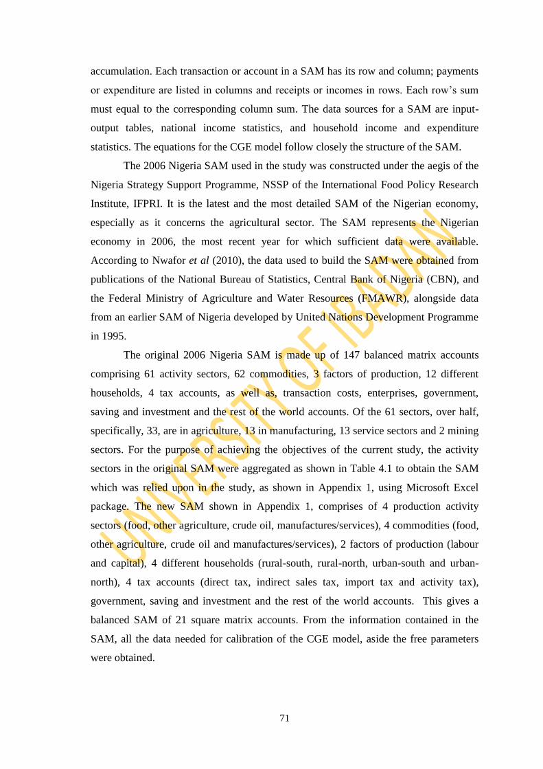
71

accumulation. Each transaction or account in a SAM has its row and column; payments

or expenditure are listed in columns and receipts or incomes in rows. Each row‘s sum

must equal to the corresponding column sum. The data sources for a SAM are input-

output tables, national income statistics, and household income and expenditure

statistics. The equations for the CGE model follow closely the structure of the SAM.

The 2006 Nigeria SAM used in the study was constructed under the aegis of the

Nigeria Strategy Support Programme, NSSP of the International Food Policy Research

Institute, IFPRI. It is the latest and the most detailed SAM of the Nigerian economy,

especially as it concerns the agricultural sector. The SAM represents the Nigerian

economy in 2006, the most recent year for which sufficient data were available.

According to Nwafor et al (2010), the data used to build the SAM were obtained from

publications of the National Bureau of Statistics, Central Bank of Nigeria (CBN), and

the Federal Ministry of Agriculture and Water Resources (FMAWR), alongside data

from an earlier SAM of Nigeria developed by United Nations Development Programme

in 1995.

The original 2006 Nigeria SAM is made up of 147 balanced matrix accounts

comprising 61 activity sectors, 62 commodities, 3 factors of production, 12 different

households, 4 tax accounts, as well as, transaction costs, enterprises, government,

saving and investment and the rest of the world accounts. Of the 61 sectors, over half,

specifically, 33, are in agriculture, 13 in manufacturing, 13 service sectors and 2 mining

sectors. For the purpose of achieving the objectives of the current study, the activity

sectors in the original SAM were aggregated as shown in Table 4.1 to obtain the SAM

which was relied upon in the study, as shown in Appendix 1, using Microsoft Excel

package. The new SAM shown in Appendix 1, comprises of 4 production activity

sectors (food, other agriculture, crude oil, manufactures/services), 4 commodities (food,

other agriculture, crude oil and manufactures/services), 2 factors of production (labour

and capital), 4 different households (rural-south, rural-north, urban-south and urban-

north), 4 tax accounts (direct tax, indirect sales tax, import tax and activity tax),

government, saving and investment and the rest of the world accounts. This gives a

balanced SAM of 21 square matrix accounts. From the information contained in the

SAM, all the data needed for calibration of the CGE model, aside the free parameters

were obtained.

72

Table 4.1: Aggregation of Sectors in the Original into Sectors in the New SAM

Sectors in the Original SAM Sectors in the

New SAM

(1) Rice (2) Wheat (3) Maize (4) Sorghum (5) Millet (6) Cassava

(7) Yams (8) Cocoyam (9) Irish Potato (10) Sweet Potato (11) Banana

and Plantain (12) Beans (13) Groundnuts (14) Soybeans (15) Beniseed

(16) Vegetables (17) Fruits (18) Cattle (19) Live Goats and Sheep

(20) Live Poultry (21) Other Livestock (22) Fish/Fish meat

Food

(23) Cocoa (24) Coffee (25) Cotton (26) Oil Palm (27) Sugarcane (28)

Unprocessed Tobacco (29) Nuts (30) Cashew (31) Rubber (32) Other

unspecified crops (33) Forestry

Other

Agriculture

(34) Crude Petroleum and Natural Gas Crude Oil

(35) Beef (36) Goat and Sheep meat (37) Poultry meat (38) Eggs (39)

Milk (40) Other meat (41) Beverages (42) Other Processed food

products (43) Textiles (44) Wood, Wood Products, Furniture (45)

Transportation and Other Equipment (46) Other Manufacturing (47)

Refined oil (48) Other mining (49) Building and Construction (50)

Electricity and Water (51)Road Transport (52) Other Transportation

(53) Wholesale and Retail Trade (54) Hotel and Restaurants (55)

Telecommunications, Post, Broadcasting (56) Finance and Other

Business Services (57) Real Estate (58) Education (59) Health (60)

Public Administration (61) Other Private Services

Manufactures/

Services

Source: Nigeria SAM, 2006

4.2.2 Nigeria Living Standards Survey Data

In addition to the SAM data, the study made use of household expenditure data

from the Nigeria Living Standards Survey of 2004, to carry out poverty and inequality

analyses. The choice of expenditure over income is informed from the fact that it has

been oft-cited that expenditure is better suited than income as indicator of wellbeing,

particularly in many developing countries. This is perhaps because, instantaneous utility

depends directly on consumption and not income per se, and again, current

consumption may also be a better indicator of long-term average well-being, as it will

73

reveal information about incomes at other dates, in the past and future (see for instance,

Ajakaiye and Adeyeye, 2002; Coudouel, et al, (2002); Duclos and Araar, 2006).

The NLSS was conducted by the National Bureau of Statistics in urban and rural

areas in the 36 states of the Federation plus the Federal Capital Territory, FCT. The

survey made use of a two-stage cluster sampling technique. The first stage was a cluster

of housing units called Enumeration Area (EA), while the second stage was the housing

unit. A total of one hundred and twenty EAs were selected and sensitized in each State,

while sixty were selected in the Federal Capital Territory. This implies that ten

Enumeration Areas (EAs) were studied in each of the States while 5 EAs were covered

in the FCT, every month for the one-year period. Ten EAs with five housing units were

studied per month in each State while five EAs and five housing units were studied in

the FCT. This meant that fifty housing units were canvassed per month in each State

and twenty-five in Abuja. This implied that the survey had an anticipated national

sample size of twenty-one thousand and nine hundred (21,900) HUs for the country for

the 12-month survey period. Each State had a sample size of 600 HUs, while the

Federal Capital Territory had a sample size of 300 (NBS, 2005). Of this sample size,

results for 19158 were reported. From this number, we disaggregated the distribution

into the four household groups in the study with the following sample sizes: 5907 for

rural south; 8605 for rural north; 2733 for urban south and 1913 for urban north. These

formed the 4 household groupings earlier mentioned in the SAM used for the study.

4.3 Analytical Framework

Two major analytical procedures were pursued in this study – the computable

general equilibrium analysis and the analysis of poverty and inequality. Since we are

studying the impact of macroeconomic shocks on households, we used the CGE model

to generate the economy-wide (or macro) impacts of the shocks on households‘ incomes

and expenditures. This is because macroeconomic shocks are economy-wide in nature

and are characterised by strong general equilibrium effects, and thus, are preferably

studied in the context of a computable general equilibrium (CGE) model, based on

national accounting data. In contrast, poverty and inequality issues are generally

analysed on the basis of household or individual (micro) data, in recognition of their

heterogeneity and the importance of capturing their full distribution (see, Cockburn,

Decaluwe and Robihaud, 2008).

74

Consequently, in the current study, these two approaches are bonded together in a

macro-micro modelling framework, which explicitly integrates household categories

into a CGE model, to obtain the extended representative household (ERH) model, a

popular approach in general equilibrium analysis of distributional implications of

macroeconomic shocks and policies (see, variously, Cockburn, 2001; Bhasin and

Obeng, 2004; Essama-Nssah, 2005).

With some modifications, this study adopted the ERH approach proposed by

Decaluwe et al (1999) and applied to Ghana by Bashin and Obeng (2004) and (2005),

Cameroon by Decaluwe, Savard and Thorbecke (2005), Cote d‘Ivoire by Aka (2006),

and Ethoipia by Aredo, Fekadu and Workneh (2008), among others. One of the key

features of the model is that the poverty line is endogenized, and so it changes with

changes in relative prices in the CGE model following an exogenous shock. This allows

us to by-pass the problem of constructing and re-constructing (outside the model)

poverty lines used in poverty analysis after each simulation run.

The actual implementation of this modelling approach involved two major steps.

First, a CGE model, based on the 2006 social accounting matrix (SAM) for Nigeria,

containing four representative household groups from the Nigeria Living Standards

Survey (NLSS), was built. This allowed us to get the benchmark equilibrium (base)

solution to the model and to perform simulation experiments, in order to mimic the

impact of the exogenous shocks considered in the study. From the simulations, we

obtain the average household income/expenditure variations following a shock as

estimated at the household category level in the CGE model. In the second step, the

income/expenditure variations were then applied to individual households within each

category using base-year income/expenditure data from the (NLSS) household survey.

The resulting new income/expenditure values were then compared with initial

income/expenditure values through the estimation of standard Foster-Greer-Thorbecke

(FGT) poverty indicators and the Gini index for inequality. This allowed us to calculate

the impact of the shocks before and after the simulations.

4.3.1 Model Specification

4.3.1.1 Specification and Description of the CGE Model for the Study

The CGE model for this study is inspired by the class of poverty-based models of

the Poverty and Economic Policy Network (see, for instance, Decaluwe et al (1999) and

2005; Cockburn et al, 2008; etc) and was calibrated on the 2006 Nigeria SAM by the

75

International Food Policy Research Institute (IFPRI), using techniques advanced by the

Global Economic Modelling (EcoMod) Network CGE model for a small open economy

(EcoMod, 2010). The model employs the standard assumptions, and assumes that

producers maximize profits subject to production functions, while households maximize

utility subject to budget constraints. Furthermore, factors are mobile across activities,

available in fixed supplies, and demanded by producers at market clearing prices. The

model satisfies Walras‘ law in that the set of commodity market equilibrium conditions

are functionally dependent, and it is homogenous of degree zero in prices.

The model is made up of four sectors (food, other agriculture, crude oil as well as

manufactures/services), two factors of production (labour and capital), and four

household categories (rural-north, rural-south, urban-north and urban-south

households). The geographical structure of the country, socioeconomic characteristics

and the availability of reliable data, mainly defined the grouping. The model comprises

six blocks of equations describing production and factor demand, income and savings,

demand for commodities, prices, international trade as well as equilibrium and market

clearing. Next, we present a listing of the model parameters, variables and equations,

followed by a description of the model equations by block.

4.3.1.1.1 Definition of Parameters and Variables in the CGE Model

In this subsection, the definitions of the model parameters, endogenous

variables, exogenous variables and definition of sets, is presented.

A: PARAMETERS

Production Functions

= Constant elasticity of substitution (CES) distribution parameter in the

production function of firm

= Efficiency parameter of CES production function of firm

= Technical coefficients (Leontief Production Function)

Constant elasticity of substitution (CES) Function between Capital and Labour

= CES capital-labour substitution-elasticities of firm

Constant elasticity of substitution (CES) Function between Imports and Domestic

Production

= CES distribution parameter of ARMINGTON function of commodity

= Efficiency parameter of ARMINGTON function of commodity

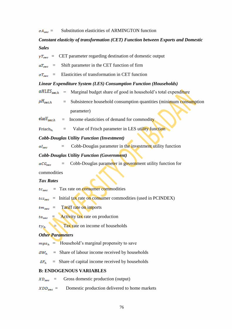
76

= Substitution elasticities of ARMINGTON function

Constant elasticity of transformation (CET) Function between Exports and Domestic

Sales

= CET parameter regarding destination of domestic output

= Shift parameter in the CET function of firm

= Elasticities of transformation in CET function

Linear Expenditure System (LES) Consumption Function (Households)

= Marginal budget share of good in household‘s total expenditure

= Subsistence household consumption quantities (minimum consumption

parameter)

= Income elasticities of demand for commodity

= Value of Frisch parameter in LES utility function

Cobb-Douglas Utility Function (Investment)

= Cobb-Douglas parameter in the investment utility function

Cobb-Douglas Utility Function (Government)

= Cobb-Douglas parameter in government utility function for

commodities

Tax Rates

= Tax rate on consumer commodities

= Initial tax rate on consumer commodities (used in PCINDEX)

= Tariff rate on imports

= Activity tax rate on production

= Tax rate on income of households

Other Parameters

= Household‘s marginal propensity to save

= Share of labour income received by households

= Share of capital income received by households

B: ENDOGENOUS VARIABLES

= Gross domestic production (output)

= Domestic production delivered to home markets

77

= Domestic sales of composite commodity

= Capital demand by sector

= Labour demand by sector

= Return to capital

= Consumer price index (commodities)

= Price level of domestic output of firm

= Price of domestic output delivered to home market

= Price level of domestic sales of composite commodities

= Import price excluding tariffs in local currency

= Price of exports in local currency

= Investment demand

= Government commodity demand

= Consumer demand for commodities

= Household expenditure (commodities)

= Export supply

= Import demand

= Household income level

= Household disposable income

= Household total income

= Total savings

= Household savings

= Total household savings

= Total government tax revenues

= Total government income

= Tax revenue on consumer commodities

= Activity tax revenue

= Tax revenue on imports

= Income tax revenue

= Objective variable

78

C: EXOGENOUS VARIABLES

= Government savings

= Foreign savings

= Capital endowment

= Supply of labour

= Wage rate

= Exchange rate

= World price of exports

= World price of imports

= Dividends paid to government

= Dividends paid to foreigners

= Total dividends paid to government and foreigners

= Total foreign transfers

= Foreign transfers to government

= Foreign transfers to households

= Government transfers to households

D: SETS

(Food, Other agriculture, Crude oil, Manufactures/services) All

activities and commodities

(Rural-south, Rural-north, Urban-south, Urban-north) Households

4.3.1.1.2 Equations in the CGE Model for Nigeria

This subsection presents the equations of the CGE model as well as a description of the

equations by block, as highlighted in subsection 4.3.1.1, above.

A. Production and Factor Demand

The production system in the model is nested; at the top level of aggregation, value-

added and intermediate inputs combine in fixed proportions, via a Leontief aggregator

function to produce gross sectoral output. At the next level of aggregation, value-added

is a constant returns to scale constant elasticity of substitution (CES) function of labour

and capital, as factors of production and intermediate inputs in Leontief technology.

From the above-named functions, the demand equations for labour and capital as well

79

as the zero-profit condition for firms, which define the firms‘ behaviour in the model,

are derived. The resulting equations are shown in equations 1-3 below:

Capital demand function for firms

1.

Labour demand function for firms

2.

Zero profit condition for the firms

3.

B. Income and Savings

In this model, households derive their income from three sources: primary factor

payments, transfers from the government and transfers from the rest of the world. From

this income, we derive the disposable income by subtracting the direct taxes collected

by the government. Household savings is specified as a fixed proportion of household‘s

disposable income. Government revenue is generated from direct taxes collected on

household income, indirect taxes on domestic goods and production activities, and taxes

levied on imports, plus dividends paid to government as well as foreign transfers to

government. Government savings are obtained from the difference between government

income and expenditures; made up of government consumption and transfers made to

households. Income and savings block is depicted in equations 4 to 16 below.

Household income

4.

Household disposable income

5.

Total household income

6.

Household savings

7.

Total household savings

8.

80

Total tax revenues

9.

Government income

10.

Government savings

11.

Total savings

12.

Activity tax Income

13.

Import tax Income

14.

Sales tax Income

15.

Income tax revenue

16.

C. Demand for Commodities

The demand system adopted in this study is the Stone-Geary linear expenditure

system (LES), which is better suited for poverty analysis since it allows us to

differentiate between minimum (subsistence) consumption and discretionary

consumption. The consumption function of households is obtained by maximization of

this system as it is supposed to reflect the household utility function. This system

assumes that the demand for commodities by households is made up of two

components: minimum consumption and the discretionary consumption. In this system,

a household-specific minimum consumption bundle which represents the minimum

quantity of each of the four commodities is postulated. This system allows us to

determine the poverty line endogenously given the monetary value of the committed

minimum consumption. Household‘s total consumption expenditure is given by

household disposable income less savings. Government demand for commodities as

well as investment demand is modelled using a Cobb-Douglas utility function.

Equations 17 to 20 describe the demand for commodities block of the model.

81

Consumer demand for commodities

17.

Household expenditure on commodities

18.

Government demand for commodities

19.

Investment demand function for commodities

20.

D. Prices

The prices block of the model is given by equations 21 to 23, which define the

import price, export price and the consumer price index.

Export price equation

21.

Import price equation

22.

Consumer Price Index

23.

E. International Trade

In modelling the foreign sector, we follow the Armington (1969) assumption of

imperfect substitutability between domestically produced and imported goods, using a

CES import function. In a similar manner, exports are modelled using a constant

elasticity of transformation (CET) function, with the believe that exports are also not

perfect substitutes for domestically produced goods in importing countries, thus

characterising the relative facility of a producer to switch between producing for the

domestic and foreign markets. This behaviour is described using the equations of import

demand, export supply, demand for domestic goods, supply of domestic goods and the

accompanying Armington zero-profit and CET zero-profit conditions in equations 24 to

29.

82

Export supply

24.

Domestic supply of domestic goods

25.

CET zero profit condition

26.

Import demand

27.

Demand for domestic goods

28.

Armington zero profit condition

29.

F. Equilibrium, Market Clearing and Model Closures

In this model, we ensure equilibrium in the factor markets for labour and capital,

product markets for the commodities as well as balance of payments equilibrium of the

foreign sector. Equations 30 to 33 describe these conditions. Equations 30 and 31

define equilibrium in the factor market for labour and capital respectively. In equation

30, market clearing requires that total labour demand equals the supply of labour.

Similarly, total capital demand, in equation 31, equals capital supply plus total capital

dividends paid to government and foreigners. The second market clearing condition

(equation 32) imposes equality between composite supply and the sum of final demand

83

for commodities. Finally, equation 33 assures balance of payment equilibrium by

equating total foreign receipts to payments. This condition equalizes the sum of imports

plus the payments to foreign capital with sum of total exports, total foreign transfers to

the government and households and foreign savings.

We assume, in traditional fashion, that the economy has no impact on international

markets, and so takes the world prices as given. Thus, world prices of imports and

exports and dividends paid to the rest of the world are exogenously fixed. The next

closure condition is that the supply of labour and capital are also exogenous to the

model. Also pre-determined outside of the model are the nominal exchange rate and

foreign savings, as well as, government savings and transfers to households.

Essentially, the study adopts the classical macro closure, where investment is

savings-driven; implying that total investment value adjusts to available level of

savings. This was used because with endogenous investment, total savings are

determined by applying exogenous saving rates to income of each institution in the

economy, hence total investment is then determined by savings behaviour and

consequently by the distribution of income among different households, firms and the

government (see, Cockburn et al, 2008).

Market clearing for labour

30.

Market clearing for capital

31.

Market clearing for commodities

32.

Balance of payments

33.

Equation 34 is used to verify Walras‘ law, and the variable Walras is thus a check

variable, which should be zero, if every equation in the model is satisfied and a general

equilibrium solution, found. Lastly, equation 35 specifies the objective function that is

to be optimized since we specify the model as a system of non-linear programming

(NLP) equations, which are solved simultaneously.

Verification of Walras Law

34.

84

Objective Function

35.

4.3.1.1.3 Calibration of the CGE Model

In order that the CGE model replicates the data represented in the base year

equilibrium, it has to be calibrated on the basis of such data. In the current study, the

2006 social accounting matrix for Nigeria provides the database for the calibration of

the CGE model for Nigeria, since the model is built around the said SAM. Thus,

calibration of the model consists in determining the numerical values of the various

parameters of the functions (production, consumption, import, export function, etc.)

compatible with the equilibrium of the initial SAM (Annabi, Cockburn and Decaluwe,

2009 and Adenikinji, 2009).These parameters, which are mostly elasticities,

propensities, ratios, etc., are assigned to equations of the CGE model in order to

guarantee that the benchmark dataset (the 2006 SAM, in our case) is the equilibrium

solution to the model. This condition, among others, has to be met, necessarily, for

simulation experiments to be carried out on the model. Apart from calculating the

elasticities from the various functions in the CGE model, the calibration exercise also

involves the calculation of tax rates, saving rates and other parameters that are needed

for the benchmark equilibrium solution to be attained.

In the current study, the ―free‖ parameters (those that cannot be calibrated from the

underlying SAM) were chosen from the literature (see, for instance Dorosh, 1996;

Yusuf, 1999; Nwafor et al, 2005; Annabi et al, 2009; etc). They include CES capital-

labour substitution elasticities, substitution elasticities of Armington function,

elasticities of transformation in the CET function as well as income elasticities of

demand for commodities. Some of the elasticities for production, consumption and

trade were the best guesstimates based on similar studies and also defined to ensure

overall model consistency (Busari, 2009). The Frisch parameter was also obtain outside

the SAM (see, Dervis, et al, 1983; Savard, 2003; Adenikinju, et al, 2009; among many).

On the basis of the obtained free parameters, we proceed to calibrate/calculate the

parameters as shown below:

Parameters of the LES utility function: alphaHLES and muH;

36.

85

37.

Parameters of the CES production function: gammaF and aF;

38.

39.

Parameters of the Armington function: gammaA and aA;

40.

41.

Parameters of the CET function: gammaT and aT;

42.

43.

Parameter of the Cobb-Douglas investment function: alphaI;

44.

Parameter of the Cobb-Douglas utility function of government: alphaCG

45.

Tax rates:

46.

47.

48.

49.

Other Parameters

50.

51.

52.

53.

The parameters and other variables calibrated and calculated using the expressions

listed in 36 to 53, above, alongside other benchmark data from the SAM, allowed the

86

model to be computable, of which solution replicated the initial data represented in the

SAM.

4.3.1.2 Poverty and Inequality Analyses in the Study

In this module, we link the macroeconomic CGE model to microeconomic

behaviour of the households, as captured in the household survey. This was done, as

mentioned earlier, by using the results (average income/expenditure values) obtained

from the base equilibrium as well as the simulations of the macro model on the

household groups in the model, to change the values of the income/expenditure data in

the household survey before carrying out poverty and inequality analyses.

The theoretical basis for this exercise is that value-added is channelled from the

production process into the income of different types of households and other

institutions through the return to factors of production owned by the households. Each

factor of production generates different amounts of value-added depending on the return

to that factor and the quantity used in the economy. Thus, differences in ownership,

types, and the value-added generated by the different factors of production determine

the distribution of income across household groups, following an economic shock, as a

result of changes in the return to factors of production or adjustments in the quantity of

the factors used in the economy or both (see, Damuri and Perdana (2003); Boccanfuso

and Savard, 2003 & 2005).

Subsequently, we describe how the estimations were carried using the results

obtained from both the base solution and scenario experiments from the CGE model to

estimate poverty measures and analyse inequality, with a view of assessing the impact

of the various shocks on these indexes, as part of the specific objectives of the study.

4.3.1.2.1 Poverty Analysis

In this study, we adopted the Foster, Greer and Thorbecke (1984) class of poverty

measures for the analysis of poverty, as in most of the CGE studies cited in section 4.3

and others including Damuri and Perdana (2003); Boccanfuso and Savard (2003) and

(2005). The choice of this measure is informed by the fact that it is additively

decomposable, and thus it allows the decomposability of the overall population into

sub-groups which helps us to making useful poverty comparisons.

The Foster-Greer-Thorbecke (FGT) index allows us to measure the proportion of the

poor in the population (the headcount ratio). Furthermore, it provides a measure of the

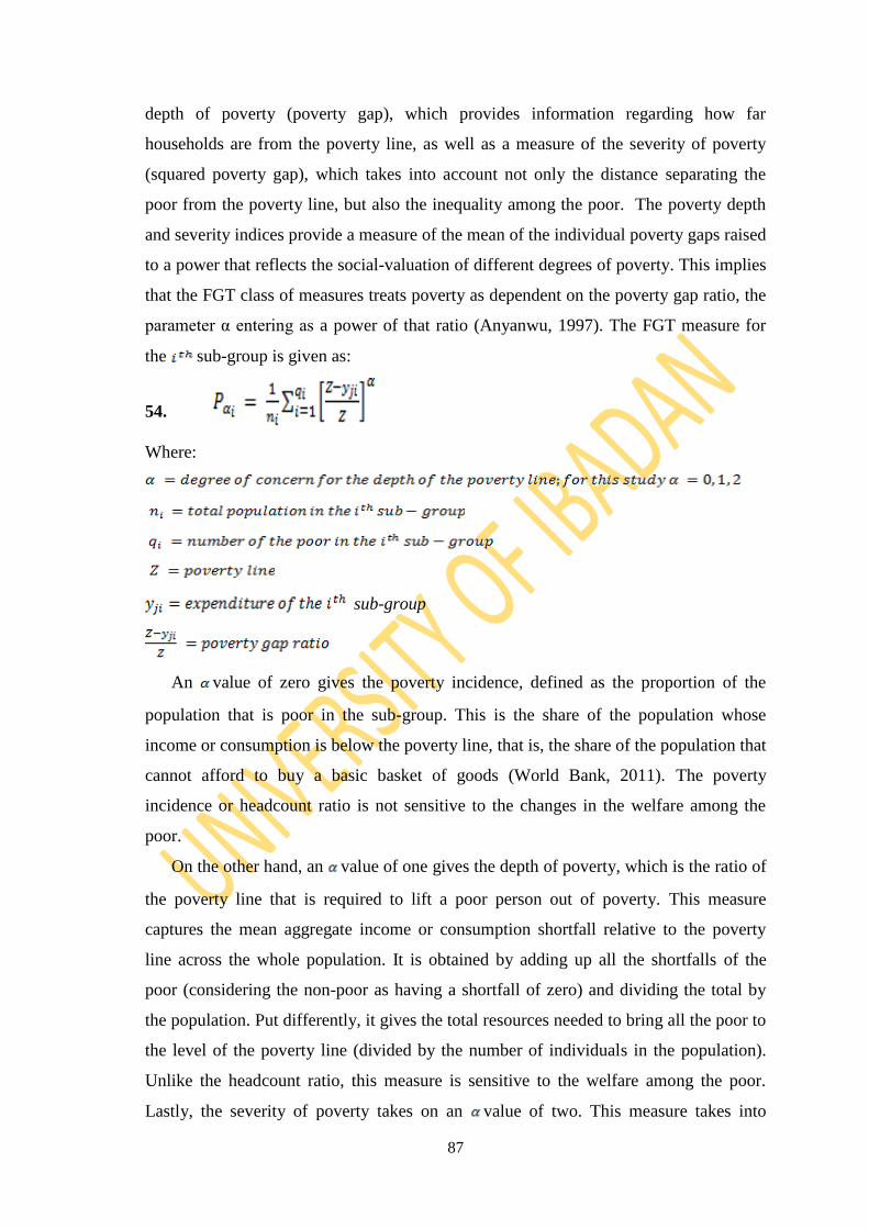
87

depth of poverty (poverty gap), which provides information regarding how far

households are from the poverty line, as well as a measure of the severity of poverty

(squared poverty gap), which takes into account not only the distance separating the

poor from the poverty line, but also the inequality among the poor. The poverty depth

and severity indices provide a measure of the mean of the individual poverty gaps raised

to a power that reflects the social-valuation of different degrees of poverty. This implies

that the FGT class of measures treats poverty as dependent on the poverty gap ratio, the

parameter α entering as a power of that ratio (Anyanwu, 1997). The FGT measure for

the sub-group is given as:

54.

Where:

sub-group

An value of zero gives the poverty incidence, defined as the proportion of the

population that is poor in the sub-group. This is the share of the population whose

income or consumption is below the poverty line, that is, the share of the population that

cannot afford to buy a basic basket of goods (World Bank, 2011). The poverty

incidence or headcount ratio is not sensitive to the changes in the welfare among the

poor.

On the other hand, an value of one gives the depth of poverty, which is the ratio of

the poverty line that is required to lift a poor person out of poverty. This measure

captures the mean aggregate income or consumption shortfall relative to the poverty

line across the whole population. It is obtained by adding up all the shortfalls of the

poor (considering the non-poor as having a shortfall of zero) and dividing the total by

the population. Put differently, it gives the total resources needed to bring all the poor to

the level of the poverty line (divided by the number of individuals in the population).

Unlike the headcount ratio, this measure is sensitive to the welfare among the poor.

Lastly, the severity of poverty takes on an value of two. This measure takes into

88

account not only the distance separating the poor from the poverty line (the poverty

gap), but also the inequality among the poor. That is, a higher weight is placed on those

households who are further away from the poverty line. As for the poverty gap measure,

limitations apply to some non-monetary indicators. As increases, more importance is

given to the shortfalls of the poorest households and the measure becomes more

distributionally sensitive.

In implementing this approach in the context of a CGE model, two points need be

resounded. First, the endogenized poverty line in the LES demand function in the CGE

model provides the poverty lines for poverty analyses in the pre- and post-shock

scenarios, as earlier indicated, thus sidestepping the arbitrariness that the construction of

a poverty line is usually fraught with (see for instance, Decaluwe et al, 1999; Decaluwe

et al, 2005; Boccanfuso and Savard, 2005; Damuri & Perdana, 2003). Second, from the

simulations of the general equilibrium model, new values with respect to average

income or expenditure levels of each of the household groups are obtained, and the

average variations are thus applied to the household distributions from the survey, this

hence allows us to calculate the indicators of poverty following an exogenous shock

(Decaluwe et al, 2005).

4.3.1.2.2 Inequality Analysis

Here, we analyse the changes in inequality in income distribution, nationally and for

the various household groups in the base year, and nationally for the post-shock

scenarios. The reason for the latter is intuitive in the sense that the simulations affect

only the average income or expenditure of each household group, and not the variance

of the income or expenditure distribution within the group. Thus, the distributional

aspects of the simulations come from the fact that the overall distribution of income or

expenditure of the entire population will change because the change of average income

and expenditure varies between one household group and another (see for example,

Damuri and Perdana, 2003).

We measure income inequality using the Gini coefficient. The Gini index was

chosen because it satisfies most of the desirable axioms of a good inequality measure, as

stated in section 2.4.1, and it is the most frequently used index to assess the rate of

overall inequality (see Decaluwe, Dumont and Savard, 1999; Abdelkrim and Awoyemi,

2006; Boccanfuso and Savard, 2005 & 2009; Aigbokahn, 2008; among others) . The

index is given as:

89

55.

Where:

The value of the Gini coefficient lies between 0 and 1, and the larger its value, the

greater the level of inequality in the distribution of income, whereas a value of zero

indicates an egalitarian income distribution or perfect equality, a value of 1 indicates

extreme inequality.

4.3.2 Model Implementation Procedures

As indicated earlier, two sets of analyses (CGE and poverty and inequality) were

carried out in order to meet the objectives of this study. The computable general

equilibrium analysis was carried out with the aid of the General Algebraic Modelling

System (GAMS) software package, by GAMS Development Corporation (2009), while

the poverty and inequality analysis was conducted using the Software for Distributive

Analysis (DAD) developed by Duclos, Araar and Fortin (2008). Next we briefly explain

how both software packages were deployed.

4.3.2.1 CGE Analysis (GAMS)

General Algebraic Modelling System (GAMS) provides high-level language for

the compact presentation of large and complex models and allows changes to be made

in model specification simply and safely. It also allows unambiguous statement of

algebraic relations and permits model descriptions that are independent of solution

algorithms (see, Oyeranti, 2005). This makes GAMS one of the best-suited packages for

the implementation of CGE models, given their high data demands and computational

complexities. Other packages include, but not limited to, GEMPACK, EVIEWS and

EXCEL.

Generally, every GAMS model follows a basic structure, which is divided into

three broad headings namely, Data, Model and Solution.

Under Data, the following tasks are performed:

i. sets declarations and definitions

90

ii. parameter declarations and definitions

iii. assignment of initial values; and

iv. displays (basically intermediate displays).

The Model comprises:

i. variable declarations

ii. equations declarations

iii. equations definitions; and

iv. model definition.

Finally, the Solution algorithm is made up of

i. solve statement; and

ii. display statements.

Following the above structure, the data for the implementation of the CGE model

from our SAM were entered after declaring sets and parameters (both scalars and

variables (exogenous and endogenous)). After this stage, the initial values from the

SAM and from the calibration process were assigned to the declared parameters so as to

enable GAMS to solve the model and replicate the base solution represented in the

SAM, then we display the assignments to ensure that the values are consistent with

those in the SAM and/or provided by calculations outside of the SAM based on the

specified expressions.

Next, we set up the model by first declaring the variables, followed by equations

declaration and specification (it should be noted that the number of endogenous

variables must be equal the number of equations to ensure that the model is a square

system, which is a requirement that assures a solution), the model was then defined (for

the current study, the model was named: ―Macroeconomic Shocks and Poverty‖ and

GAMS was asked to solve the equations listed inside the two slashes (―//‖) after the

model name in GAMS syntax).

The last part of the model structure is the Solution. Here, we specified the solve

statement, which reads: ―Solve Macroeconomic Shocks and Poverty using NLP

maximizing OMEGA‖. NLP here stands for Non-Linear Programming. So, we used an

NLP Solver called CONOPT3 (the most recent version of CONOPT solver at the time)

to solve the system of equations since the model was specified as a system of non-linear

equations with an objective function OMEGA (see equation 35) to be optimized, in this

case by maximization. Finally, we ask GAMS to display the results, which must exactly

91

replicate the benchmark data provided to GAMS. This can only be obtained if all the

model equations are satisfied, system is square, the calibration was successful, and in

which case GAMS would return a ―normal completion‖ and ―locally optimal‖ solution

for an NLP problem, like in the current one. The interested reader can request for the

GAMS code for details on the model structure.

The model was specified and solved in a comparative static mode. Upon solving

for the benchmark equilibrium, it provided a simulation laboratory, which allowed us to

carry out ‗controlled‘ experiments, changing the exogenous conditions (using the

shocks pursued in this study), and then measuring the impact against the baseline

conditions. Each solution provides a full set of economic indicators, including

household incomes, expenditures; prices, supplies, and demands for factors and

commodities, etc as well as macroeconomic results.

4.3.2.2 Poverty and Inequality Analysis (DAD)

The software for Distributive Analysis, DAD is one of the widely used packages for

poverty and inequality analyses in recent times, particularly because of its user-friendly

interface and the fact that it is freely available. We deployed it in the analysis of poverty

indexes before and after shocks to the CGE model and to analyse pre- and post-shock

inequality of the four household categories and Nigeria as a whole (see Savard, 2003).

For poverty analysis, we used the household expenditure data from the NLSS, for

Nigeria as a whole, and for the four household categories in addition to the poverty lines

obtained from the CGE model, to estimate poverty incidence, depth and severity using

the FGT class of poverty measures. Similarly, we used the same expenditure data to

analyse inequality for the four household groups and Nigeria as whole.

4.3.3 Description of and Rationale for Model Simulation Experiments

The policy scenarios in the study were chosen to, as much as possible mimic the

macroeconomic shocks that impacted the economy in the wake of the global economic

crisis, variously and in combination, with a view to capturing their effects on poverty

and household inequality. Apart from other shocks, rise in world prices of food

imports, fall in world price of oil exports, and exchange rate depreciation were

prominent and so, we simulated the model under the following alternative scenarios,

having successfully replicated the benchmark equilibrium:

i. 50% rise in the world price of food imports

92

ii. 50% fall in the world price of oil exports

iii. 25% depreciation of the real exchange rate

iv. Combination of scenarios i, ii and iii above.

Although the focus of the discussion in this study is on the simulation experiments,

which were based on the negative shocks outlined above, but in order to appreciate the

impact of the above-named simulations in terms of a broader picture, we also simulated

the reverse scenarios, which represent positive shocks, to see what would be the case if

the opposite had occurred. Thus, the second set of simulations (which were only

highlighted but not discussed, since they were not the focus of the study) includes:

a. 50% fall in the world price of food imports

b. 50% rise in the world price of oil exports

c. 25% appreciation of the real exchange rate

d. Combination of scenarios a, b and c above.

Furthermore, the levels of the experiments were taken to represent as close as

possible the levels of the shocks that impacted the economy. For example, the Food and

Agriculture Organisation (FAO), reports in its food price index that food prices had

risen about 53 percent in the peak of the crisis in 2008. For the oil price, simulations,

data from the Central Bank of Nigeria (CBN) for monthly oil prices between July 2008,

which recorded the highest oil price and June, 2009 showed a total percentage price fall

in oil prices for the one-year period of 50.3 percent. Lastly, as indicated earlier, the

exchange rate had risen about 25 percent by February 2009 from its fairly stable level in

early to toward the end of 2008.

The results of the experiments and associated analyses are presented and discussed

next.

93

CHAPTER FIVE

RESULTS AND DISCUSSION

5.1 Introduction

In this chapter the results of the empirical exercise are presented followed in each

case by a discussion of the results. In section 5.2, we present the results of the

descriptive analysis of the economy at the reference period. This is followed by the base

equilibrium solution of the CGE model in section 5.3. In the next section (5.4), we

present and discuss the simulation results, which then leads us to an assessment of the

poverty status of household groups vis-à-vis the nation in the base year, in section 5.5.

In section 5.6, the impact of the various simulations on poverty is presented and finally

section 5.7 concludes with the impact of the simulations on inequality.

5.2 Descriptive Analysis of the Structure of the Economy in the Base Year

We begin with the presentation and discussion of the results describing the basic

structure of the Nigeria economy in the base year before the shocks. This is necessary

because the structure of the economy has important poverty and distributional

ramifications. It also allows us to have an understanding of how and what sectors or

households would be affected by the various shocks applied to the model.

5.2.1 Sources of Household Income

Table 5.1 shows the sources from which households derived their incomes, as well

as the population of each household group and the average amount of income earned

per person in a year. From the table, urban-south households, which represent almost 25

percent of the population, earned the highest amount of income of N154,000.433 per

head while rural-north households that make up almost 34 percent of the population,

earned the lowest income of N77,062.578 per capita. Urban-north and rural-south

households, which represented about 19.5 and 22 percent earned N141,371.992 and

N85,421.051 per head per annum, respectively. Clearly, the average incomes were

found to be very low: N85,421.051 for rural-south households and N77,062.578 for

rural-north households, per person per year. These average incomes translate into

N234.03 (or US$1.56) and N211.13 (or US$1.41) per day for rural-south and rural-

north households respectively, which are less than all the endogenous poverty lines used

in the study.

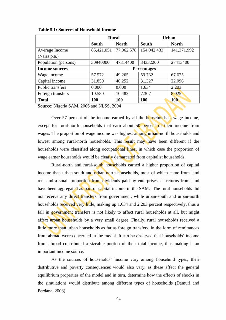
94

Table 5.1: Sources of Household Income

Rural Urban

South North South North

Average Income

(Naira p.a.)

85,421.051 77,062.578 154,042.433 141,371.992

Population (persons) 30940000 47314400 34332200 27413400

Income sources Percentages

Wage income 57.572 49.265 59.732 67.675

Capital income 31.850 40.252 31.327 22.096

Public transfers 0.000 0.000 1.634 2.203

Foreign transfers 10.580 10.482 7.307 8.025

Total 100 100 100 100

Source: Nigeria SAM, 2006 and NLSS, 2004

Over 57 percent of the income earned by all the households is wage income,

except for rural-north households that earn about 50 percent of their income from

wages. The proportion of wage income was highest among urban-north households and

lowest among rural-north households. This result may have been different if the

households were classified along occupational lines, in which case the proportion of

wage earner households would be clearly demarcated from capitalist households.

Rural-north and rural-south households earned a higher proportion of capital

income than urban-south and urban-north households, most of which came from land

rent and a small proportion from dividends paid by enterprises, as returns from land

have been aggregated as part of capital income in the SAM. The rural households did

not receive any direct transfers from government, while urban-south and urban-north

households received very little, making up 1.634 and 2.203 percent respectively, thus a

fall in government transfers is not likely to affect rural households at all, but might

affect urban households by a very small degree. Finally, rural households received a

little more than urban households as far as foreign transfers, in the form of remittances

from abroad were concerned in the model. It can be observed that households‘ income

from abroad contributed a sizeable portion of their total income, thus making it an

important income source.

As the sources of households‘ income vary among household types, their

distributive and poverty consequences would also vary, as these affect the general

equilibrium properties of the model and in turn, determine how the effects of shocks in

the simulations would distribute among different types of households (Damuri and

Perdana, 2003).

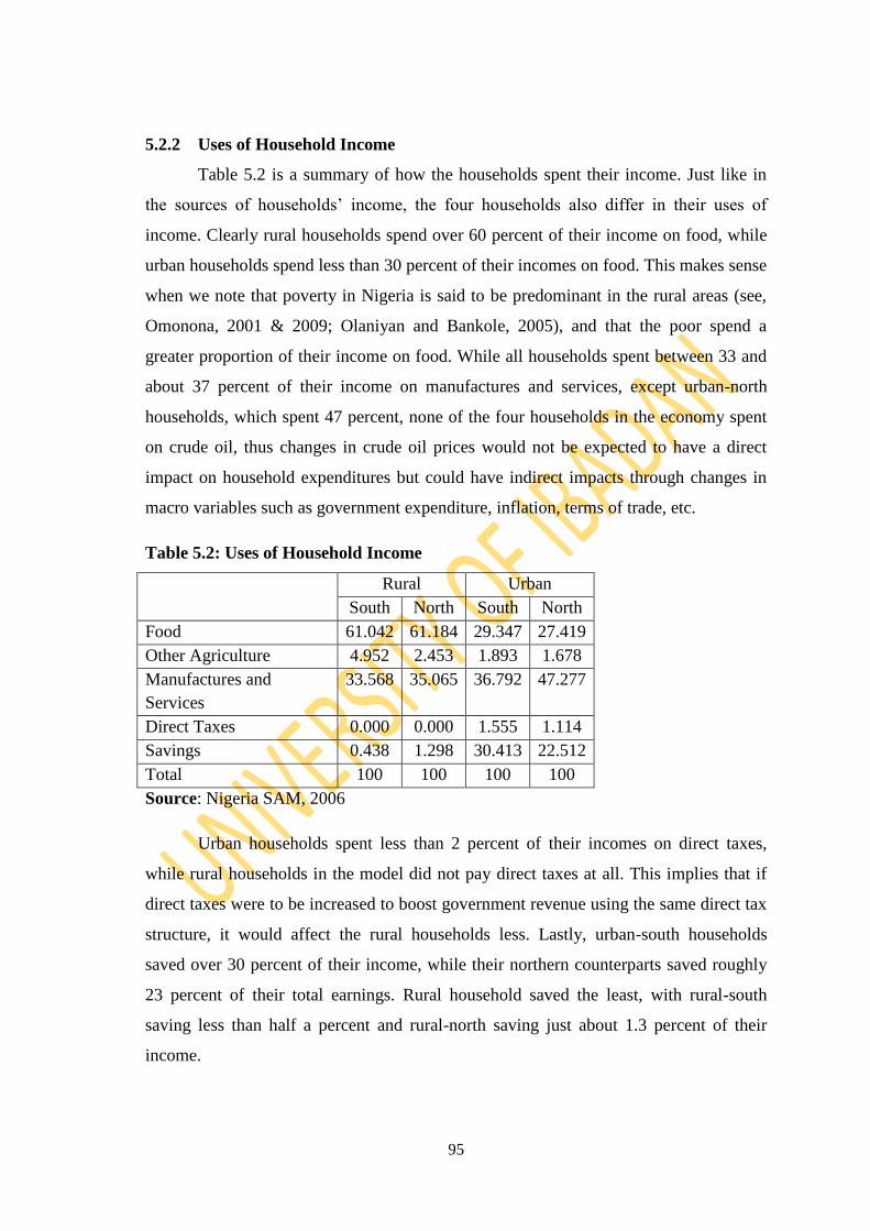
95

5.2.2 Uses of Household Income

Table 5.2 is a summary of how the households spent their income. Just like in

the sources of households‘ income, the four households also differ in their uses of

income. Clearly rural households spend over 60 percent of their income on food, while

urban households spend less than 30 percent of their incomes on food. This makes sense

when we note that poverty in Nigeria is said to be predominant in the rural areas (see,

Omonona, 2001 & 2009; Olaniyan and Bankole, 2005), and that the poor spend a

greater proportion of their income on food. While all households spent between 33 and

about 37 percent of their income on manufactures and services, except urban-north

households, which spent 47 percent, none of the four households in the economy spent

on crude oil, thus changes in crude oil prices would not be expected to have a direct

impact on household expenditures but could have indirect impacts through changes in

macro variables such as government expenditure, inflation, terms of trade, etc.

Table 5.2: Uses of Household Income

Rural Urban

South North South North

Food 61.042 61.184 29.347 27.419

Other Agriculture 4.952 2.453 1.893 1.678

Manufactures and

Services

33.568 35.065 36.792 47.277

Direct Taxes 0.000 0.000 1.555 1.114

Savings 0.438 1.298 30.413 22.512

Total 100 100 100 100

Source: Nigeria SAM, 2006

Urban households spent less than 2 percent of their incomes on direct taxes,

while rural households in the model did not pay direct taxes at all. This implies that if

direct taxes were to be increased to boost government revenue using the same direct tax

structure, it would affect the rural households less. Lastly, urban-south households

saved over 30 percent of their income, while their northern counterparts saved roughly

23 percent of their total earnings. Rural household saved the least, with rural-south

saving less than half a percent and rural-north saving just about 1.3 percent of their

income.

96

5.2.3 Sectoral Factor Remunerations and Factor Market Shares

Table 5.3 serves two purposes: the upper part depicts factor remunerations by

sector while the lower portion of the table shows the share of each factor in each sector.

The remuneration of factors was highest in the manufactures and services sector, with a

total of about 36 percent of total value-added. Of this proportion, labour accounted for

61 percent whereas, capital accounted for about 14 percent. Although the crude oil

sector accounted for about 34 percent of total value-added, labour accounted for a paltry

0.2 percent while capital accounted for 63.30 percent. This again reinforces the enclave

nature of the crude oil sector, with little if any direct linkages to the rest of the Nigerian

economy (see, Akpan, 2009). The food sector accounted for about 28 percent of total

factor remunerations out of which it accounted for 36 percent of total value-added by

labour and about 21 percent of total value-added by capital.

The second part of the table shows the relative importance of each factor in each

sector. While both labour and capital were almost equally important in the food and

other agriculture sectors, the picture for the crude oil sector was remarkably different, as

almost 100 percent of value added in this sector came from capital. This indicates that

the crude oil sector is highly capital intensive, as existing capital determines the level of

output (Adenikinju and Falobi, 2006).

Table 5.3: Sectoral Factor Remunerations and Factor Market Shares

Food Other

Agriculture

Crude Oil Manufactures/

Services

Total

Labour (N‘million) 3280392.135 231495.880 18713.492 5569053.713 9099655.219

Percent 36.050 2.544 0.206 61.201 100

Capital (N‘million) 2235632.742 166128.653 6841676.961 1565438.952 10808877.31

Percent 20.683 1.537 63.300 14.483 100

Total Value Added 5516024.877 397624.533 6860390.453 7134492.665 19908532.529

Percent 27.707 1.997 34.459 35.836 100

Labour 59.470 58.220 0.272 78.058 45.707

Capital 40.530 41.780 99.730 21.942 54.293

Total Value Added 100 100 100 100 100

Source: Nigeria SAM, 2006

A contrasting picture is seen in the manufactures and services sector, where 78

percent of value-added came from labour while 22 percent came from capital. In this

model, it can be observed that labour is remunerated mostly by the

manufactures/services and food sectors, while capital is mainly derived from crude oil

sector. Thus, if the shocks, for example, favour the expansion of the food sector the

return to labour in this sector is expected to increase (see Cockburn et al, 2008).

97

5.2.4 Household Consumption and Import Intensity

Table 5.4 shows the shares of household consumption from each sector as well

as the share of import consumed by households by sector. Food accounts for over 61

percent of rural households‘ consumption, while urban households consume mainly

manufactures/services. The table also reveals that the share of imports in total

household consumption is almost 39 percent. Of this proportion, about 6 percent of

households‘ consumption of food is imported while the share of imports consumed in

Other Agriculture and manufactures/services stand at 25.74 and 75.55 percent,

respectively. The impact of the simulations on poverty and inequality would also

depend on household consumption shares in each sector and the amount of imports in

which they consume from each sector. For example, which households are mostly

affected by consumer price changes depends on their respective consumption patterns,

also reflected in how much imported or domestically produced commodities that they

consume. Thus, changes in food prices are expected to affect rural households more

than urban households, while changes in the consumer prices of manufactures/services

should affect urban households more. Differences in sectoral consumption shares imply

that changes in consumer prices of goods as a result of economic shocks would impact

household categories differently (see, Cockburn et al, 2008).

Table 5.4: Household Consumption Shares and Import Intensity

Sectors Rural Urban Sectoral Import

Shares South North South North

Food 61.311 61.989 43.137 35.901 5.82

Other Agriculture 4.974 2.485 2.782 2.200 25.74

Manufactures/Services 33.715 35.526 54.081 61.902 75.55

Total 100 100 100 100 38.83

Source: Nigeria SAM, 2006

5.2.5 Government Revenue and Expenditure

Table 5.5 above indicates that government earns over 86 percent of its income from

capital paid as dividend income by enterprises while smallest amount of government

income of less than 1 percent of total, is earned from indirect sales tax. Government

revenue, hence its expenditure can impact households through transfers and indirectly

through investment expenditure, which can impact earnings ability of households in the

long-run (see, Nwafor et al, 2007).

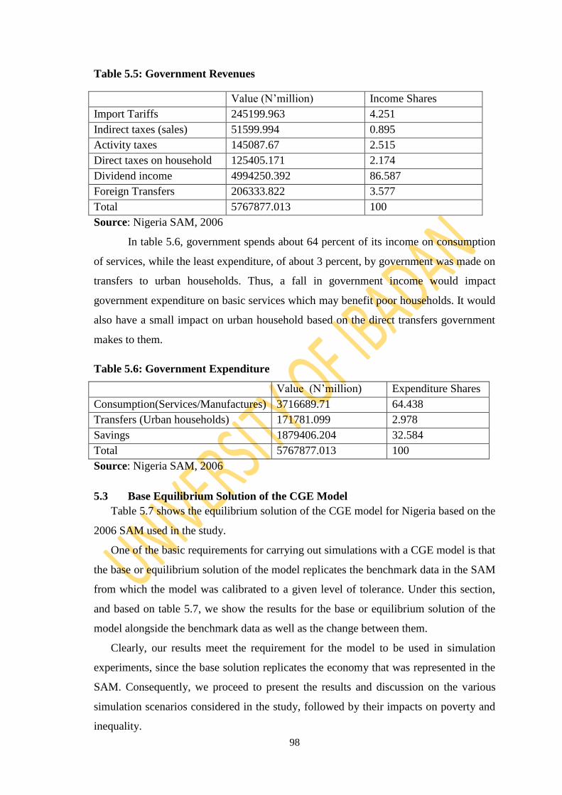
98

Table 5.5: Government Revenues

Value (N‘million) Income Shares

Import Tariffs 245199.963 4.251

Indirect taxes (sales) 51599.994 0.895

Activity taxes 145087.67 2.515

Direct taxes on household 125405.171 2.174

Dividend income 4994250.392 86.587

Foreign Transfers 206333.822 3.577

Total 5767877.013 100

Source: Nigeria SAM, 2006

In table 5.6, government spends about 64 percent of its income on consumption

of services, while the least expenditure, of about 3 percent, by government was made on

transfers to urban households. Thus, a fall in government income would impact

government expenditure on basic services which may benefit poor households. It would

also have a small impact on urban household based on the direct transfers government

makes to them.

Table 5.6: Government Expenditure

Value (N‘million) Expenditure Shares

Consumption(Services/Manufactures) 3716689.71 64.438

Transfers (Urban households) 171781.099 2.978

Savings 1879406.204 32.584

Total 5767877.013 100

Source: Nigeria SAM, 2006

5.3 Base Equilibrium Solution of the CGE Model

Table 5.7 shows the equilibrium solution of the CGE model for Nigeria based on the

2006 SAM used in the study.

One of the basic requirements for carrying out simulations with a CGE model is that

the base or equilibrium solution of the model replicates the benchmark data in the SAM

from which the model was calibrated to a given level of tolerance. Under this section,

and based on table 5.7, we show the results for the base or equilibrium solution of the

model alongside the benchmark data as well as the change between them.

Clearly, our results meet the requirement for the model to be used in simulation

experiments, since the base solution replicates the economy that was represented in the

SAM. Consequently, we proceed to present the results and discussion on the various

simulation scenarios considered in the study, followed by their impacts on poverty and

inequality.

99

Table 5.7: Replicated Benchmark Data

Variable Benchmark Data Replicated Data Change

Households

Household income

Level

Rural south 2642927.340 2642927.340 0.000

Rural north 3646169.671 3646169.671 0.000

Urban south 5288615.606 5288615.606 0.000

Urban north 3875486.962 3875486.962 0.000

Household

consumption

expenditure

Rural south 2631340.864 2631340.864 0.000

Rural north 3598827.408 3598827.408 0.000

Urban south 3597972.672 3597972.672 0.000

Urban north 2959873.227 2959873.227 0.000

Household Savings

Rural south 11586.476 11586.476 0.000

Rural north 47342.263 47342.263 0.000

Urban south 1608424.335 1608424.335 0.000

Urban north 872427.164 872427.164 0.000

Gross Domestic Output

Food 6456533.767 6456533.765 0.001

Other Agriculture 549607.182 549607.186 -0.004

Crude Oil 745559.843 745559.863 -0.020

Manufactures/Services 13083842.85 13083842.85 0.000

Domestic Production to

Home market

Food 6451123.411 6451123.349 0.006

Other Agriculture 520779.202 520779.206 -0.004

Crude Oil 118662.779 118662.781 -0.002

Manufactures/Services 12618307.4 12618307.4 0.000

Domestic Sales of

Composite commodity

Food 7019982.273 7019982.205 0.006

Other Agriculture 629509.359 629509.364 -0.005

Crude Oil 120016.423 120016.425 -0.002

Manufactures/Services 17151628.25 17151628.25 0.000

Imports

Food 375861.244 375861.240 0.004

Other Agriculture 99233.416 99233.417 -0.001

Crude Oil 1353.644 1353.644 0.000

Manufactures/Services 4490615.253 4490615.278 -0.002

Exports

Food 5410.356 5410.356 0.000

Other Agriculture 28827.980 28827.980 0.000

Crude Oil 7336897.064 7336897.083 -0.001

Manufactures/Services 465535.452 465535.454 -0.002

Source: CGE Model Solution

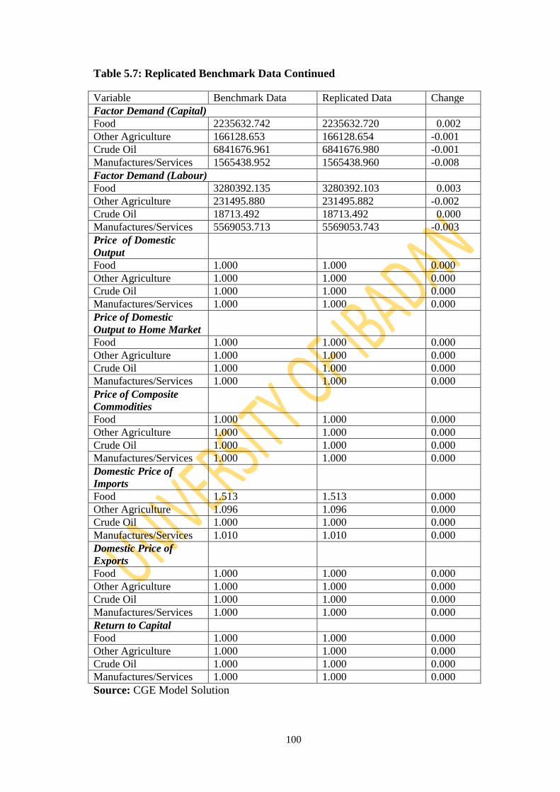
100

Table 5.7: Replicated Benchmark Data Continued

Variable Benchmark Data Replicated Data Change

Factor Demand (Capital)

Food 2235632.742 2235632.720 0.002

Other Agriculture 166128.653 166128.654 -0.001

Crude Oil 6841676.961 6841676.980 -0.001

Manufactures/Services 1565438.952 1565438.960 -0.008

Factor Demand (Labour)

Food 3280392.135 3280392.103 0.003

Other Agriculture 231495.880 231495.882 -0.002

Crude Oil 18713.492 18713.492 0.000

Manufactures/Services 5569053.713 5569053.743 -0.003

Price of Domestic

Output

Food 1.000 1.000 0.000

Other Agriculture 1.000 1.000 0.000

Crude Oil 1.000 1.000 0.000

Manufactures/Services 1.000 1.000 0.000

Price of Domestic

Output to Home Market

Food 1.000 1.000 0.000

Other Agriculture 1.000 1.000 0.000

Crude Oil 1.000 1.000 0.000

Manufactures/Services 1.000 1.000 0.000

Price of Composite

Commodities

Food 1.000 1.000 0.000

Other Agriculture 1.000 1.000 0.000

Crude Oil 1.000 1.000 0.000

Manufactures/Services 1.000 1.000 0.000

Domestic Price of

Imports

Food 1.513 1.513 0.000

Other Agriculture 1.096 1.096 0.000

Crude Oil 1.000 1.000 0.000

Manufactures/Services 1.010 1.010 0.000

Domestic Price of

Exports

Food 1.000 1.000 0.000

Other Agriculture 1.000 1.000 0.000

Crude Oil 1.000 1.000 0.000

Manufactures/Services 1.000 1.000 0.000

Return to Capital

Food 1.000 1.000 0.000

Other Agriculture 1.000 1.000 0.000

Crude Oil 1.000 1.000 0.000

Manufactures/Services 1.000 1.000 0.000

Source: CGE Model Solution

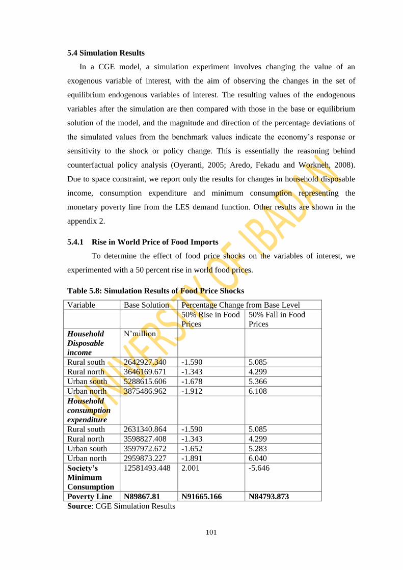
101

5.4 Simulation Results

In a CGE model, a simulation experiment involves changing the value of an

exogenous variable of interest, with the aim of observing the changes in the set of

equilibrium endogenous variables of interest. The resulting values of the endogenous

variables after the simulation are then compared with those in the base or equilibrium

solution of the model, and the magnitude and direction of the percentage deviations of

the simulated values from the benchmark values indicate the economy‘s response or

sensitivity to the shock or policy change. This is essentially the reasoning behind

counterfactual policy analysis (Oyeranti, 2005; Aredo, Fekadu and Workneh, 2008).

Due to space constraint, we report only the results for changes in household disposable

income, consumption expenditure and minimum consumption representing the

monetary poverty line from the LES demand function. Other results are shown in the

appendix 2.

5.4.1 Rise in World Price of Food Imports

To determine the effect of food price shocks on the variables of interest, we

experimented with a 50 percent rise in world food prices.

Table 5.8: Simulation Results of Food Price Shocks

Variable Base Solution Percentage Change from Base Level

50% Rise in Food

Prices

50% Fall in Food

Prices

Household

Disposable

income

N‘million

Rural south 2642927.340 -1.590 5.085

Rural north 3646169.671 -1.343 4.299

Urban south 5288615.606 -1.678 5.366

Urban north 3875486.962 -1.912 6.108

Household

consumption

expenditure

Rural south 2631340.864 -1.590 5.085

Rural north 3598827.408 -1.343 4.299

Urban south 3597972.672 -1.652 5.283

Urban north 2959873.227 -1.891 6.040

Society’s

Minimum

Consumption

12581493.448 2.001 -5.646

Poverty Line N89867.81 N91665.166 N84793.873

Source: CGE Simulation Results

102

From the results in table 5.8, a 50 percent rise in the world price of food imports

causes households disposable incomes and consumption expenditures to fall. This is as

expected and indicates that all household categories are net consumers and not net

producers of food, as this increase in price forces the price of food composites to

increase thus reducing real disposable incomes and accordingly lowering their

consumption of food. This action however, raises the minimum consumption (defined

as the nominal value of the basic needs commodity basket or the monetary poverty line)

nationally by about 2 percent due to an increase in relative prices of commodities that

constitute the basic needs basket of households. It can be noticed that the overall

increase in the national poverty line is induced by the increase in the poverty line for

rural households, who spend over 61 percent of their incomes on food compared with

less that 30 percent spent by urban households (see table 5.2). Expectedly, the impact of

this shock on poverty would be higher on rural households but this also depends on the

distributional impact of the shock. Generally, this shock is expected to increase the

poverty situation of all the households since there is both a rise in commodity prices

following the shock, and a fall in the incomes of all the households, all things being

equal.

On the other hand, a 50 percent fall in food price had the opposite effect of lowering

the poverty line by over 5 percent, a margin which is higher than the 2 percent increase

when a 50 percent rise in food price was simulated. This result indicates that lower food

prices are likely to reduce poverty by a larger margin than higher food prices would

increase it, given the margin at which the poverty line dropped when food prices were

reduced.

5.4.2 Fall in World Price of Oil Exports

In this simulation experiment, we explore the effect of a 50 percent fall the

world price of oil exports on household parameters. Conceptually, an oil price shock, in

the Nigerian case is not supposed to have direct effects on households, particularly, as a

net exporter of oil and the enclave nature of the Nigerian oil economy.

103

Table 5.9: Simulation Results of Oil Price Shocks

Variable Base Solution Percentage Change from Base Level

50% Fall in Oil

Prices

50% Rise in Oil

Prices

Household Disposable

income

Rural south 2642927.340 -1.401 6.756

Rural north 3646169.671 -6.543 10.103

Urban south 5288615.606 -0.759 6.540

Urban north 3875486.962 4.715 2.871

Household consumption

expenditure

Rural south 2631340.864 -1.401 6.756

Rural north 3598827.408 -6.543 10.103

Urban south 3597972.672 -0.747 6.438

Urban north 2959873.227 4.662 2.839

Society’s Minimum

Consumption

12581493.44

8

-1.912 10.333

Poverty Line N89867.81 N88149.53 N99159.13

Source: CGE Simulation Results

The effects are generally indirect, trickling down from the macroeconomic

repercussions of such a shock, as well as, from government spending channel, given

that crude oil constitutes more than 90 percent of Nigeria‘s export earnings and on

average about 70 percent of government revenues in annual budgets (see Akpan, 2009).

The indirect channels that a fall in oil prices can affect households include their effect

via government expenditure (inflation, transfers, spending on services, employment,

etc) and their impact through attempts to restore balance of payment equilibrium, for

example, via exchange rate depreciation. Given the above background, the impact of a

fall in the price of oil will be determined by various factors acting together. From the

results in table 5.9, a 50 percent fall in oil price reduces the disposable income of all

households, except that of urban-north households, which actually increase by almost 5

percent. Rural-north households suffer the highest reduction in incomes of over 6

percent.

A similar picture can be observed for household consumption expenditures, with

accompanying fiscal implications. In the model, this shock reduces government income,

savings and expenditure. This causes a chain of adjustments that culminate in the above

results. For instance, a fall in government revenue from oil exports due to depressed

prices leads to unfavourable terms of trade, which induces a real depreciation of the

exchange rate with attendant consequences for households that are net importers as a

result of changes in relative prices. Moreover, from the results, expenditure on services

104

which accounted for over 64 percent of government expenditure (see table 5.6) is

reduced by over 11 percent, while total savings which government savings constitutes 2

percent is reduced by 86 percent. The effect of these would distribute differently among

households. With our main interest being the poverty and distributional impacts, we

observed from the model that the poverty lines for rural households decreased while that

of urban households increased. Overall, the national poverty line dropped almost 2

percent, because of the drop in the prices of most composite goods in the economy,

which means that we might expect a reduction in poverty levels in the analysis of

poverty impacts which follows in section 5.4. These results are appealing because the

fall in government income by over 15 percent as a result of this shock is accompanied

by a reduction in government spending, which has a potential of reducing inflationary

pressures, which indirectly raises real incomes (see, Nwafor et al, 2005).

Conversely, a rise in oil price by 50 percent, which can be considered a positive

shock for a net oil exporting country like Nigeria, increases the national poverty line by

over 10 percent compared with about a 1.9 percent decrease in the case of a 50 percent

fall in oil price. This indicates that increases in oil price, as explained earlier, have the

tendency to increase the general level of prices, thus making it possible for more people

to fall below the poverty line, and thus likely to increase poverty.

5.4.3 Depreciation of the Exchange Rate

To determine the effect of exchange rate shocks on the variables of interest, we

experimented with a 25% rise in the nominal exchange rate. As noted in chapter 2, the

effect of exchange rate changes can be very significant in the economy because of its

impact on the relative prices of commodities. A real depreciation increases producer

prices for exports, with a larger impact in relatively export-oriented sectors, and

demand-side prices for imports, which boost prices of domestically produced import

substitutes. This has the effect of making exports cheaper and imports, expensive. From

the simulation results in table 5.10, exchange rate depreciation remarkably increases

households‘ disposable incomes and consumption expenditures. This is theoretically

plausible as noted by Oyeranti (2005), as Rural-north households‘ incomes increased

highest by about 17 percent, followed by urban-north (with 16 percent), rural-south

(15.7 percent) and urban-north (14 percent). A similar picture is observed for

consumption expenditures. However, the results indicate an increase in the monetary

poverty lines of rural households but a fall in the monetary poverty line of urban

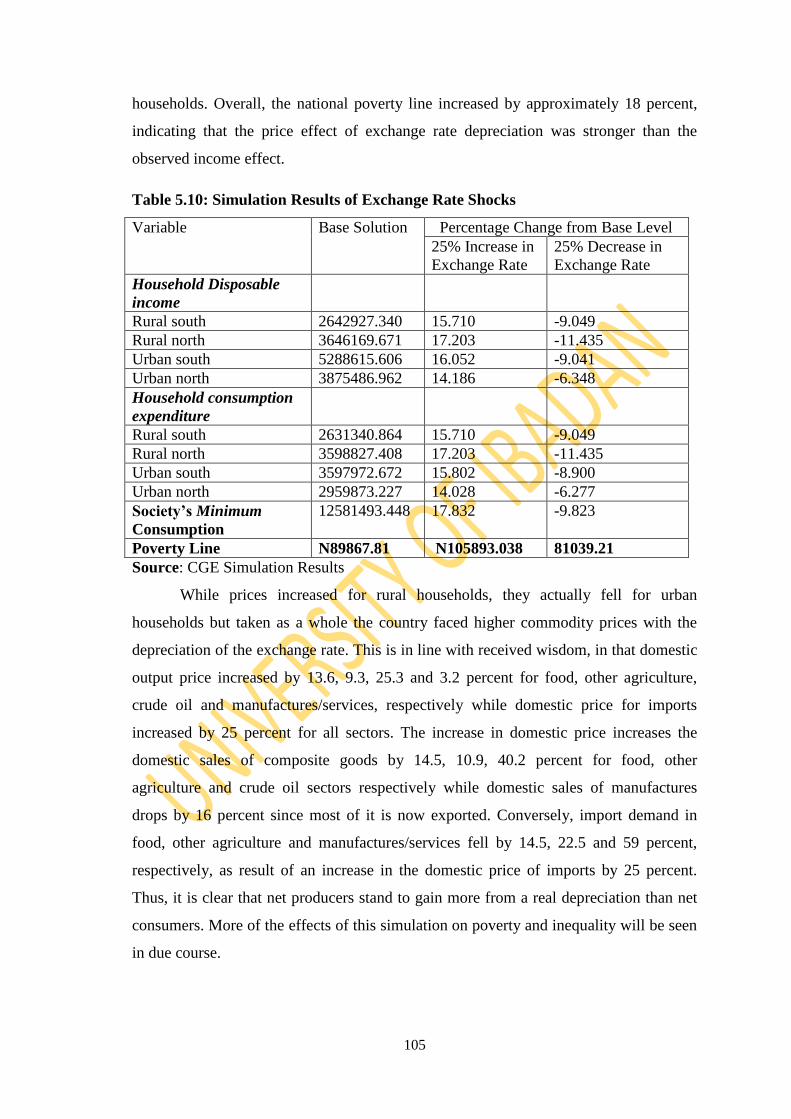
105

households. Overall, the national poverty line increased by approximately 18 percent,

indicating that the price effect of exchange rate depreciation was stronger than the

observed income effect.

Table 5.10: Simulation Results of Exchange Rate Shocks

Variable Base Solution Percentage Change from Base Level

25% Increase in

Exchange Rate

25% Decrease in

Exchange Rate

Household Disposable

income

Rural south 2642927.340 15.710 -9.049

Rural north 3646169.671 17.203 -11.435

Urban south 5288615.606 16.052 -9.041

Urban north 3875486.962 14.186 -6.348

Household consumption

expenditure

Rural south 2631340.864 15.710 -9.049

Rural north 3598827.408 17.203 -11.435

Urban south 3597972.672 15.802 -8.900

Urban north 2959873.227 14.028 -6.277

Society’s Minimum

Consumption

12581493.448 17.832 -9.823

Poverty Line N89867.81 N105893.038 81039.21

Source: CGE Simulation Results

While prices increased for rural households, they actually fell for urban

households but taken as a whole the country faced higher commodity prices with the

depreciation of the exchange rate. This is in line with received wisdom, in that domestic

output price increased by 13.6, 9.3, 25.3 and 3.2 percent for food, other agriculture,

crude oil and manufactures/services, respectively while domestic price for imports

increased by 25 percent for all sectors. The increase in domestic price increases the

domestic sales of composite goods by 14.5, 10.9, 40.2 percent for food, other

agriculture and crude oil sectors respectively while domestic sales of manufactures

drops by 16 percent since most of it is now exported. Conversely, import demand in

food, other agriculture and manufactures/services fell by 14.5, 22.5 and 59 percent,

respectively, as result of an increase in the domestic price of imports by 25 percent.

Thus, it is clear that net producers stand to gain more from a real depreciation than net

consumers. More of the effects of this simulation on poverty and inequality will be seen

in due course.

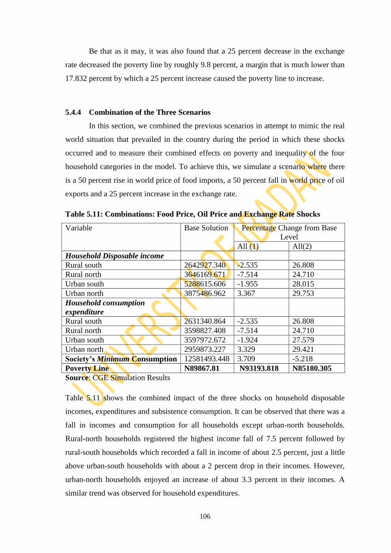
106

Be that as it may, it was also found that a 25 percent decrease in the exchange

rate decreased the poverty line by roughly 9.8 percent, a margin that is much lower than

17.832 percent by which a 25 percent increase caused the poverty line to increase.

5.4.4 Combination of the Three Scenarios

In this section, we combined the previous scenarios in attempt to mimic the real

world situation that prevailed in the country during the period in which these shocks

occurred and to measure their combined effects on poverty and inequality of the four

household categories in the model. To achieve this, we simulate a scenario where there

is a 50 percent rise in world price of food imports, a 50 percent fall in world price of oil

exports and a 25 percent increase in the exchange rate.

Table 5.11: Combinations: Food Price, Oil Price and Exchange Rate Shocks

Variable Base Solution Percentage Change from Base

Level

All (1) All(2)

Household Disposable income

Rural south 2642927.340 -2.535 26.808

Rural north 3646169.671 -7.514 24.710

Urban south 5288615.606 -1.955 28.015

Urban north 3875486.962 3.367 29.753

Household consumption

expenditure

Rural south 2631340.864 -2.535 26.808

Rural north 3598827.408 -7.514 24.710

Urban south 3597972.672 -1.924 27.579

Urban north 2959873.227 3.329 29.421

Society’s Minimum Consumption 12581493.448 3.709 -5.218

Poverty Line N89867.81 N93193.818 N85180.305

Source: CGE Simulation Results

Table 5.11 shows the combined impact of the three shocks on household disposable

incomes, expenditures and subsistence consumption. It can be observed that there was a

fall in incomes and consumption for all households except urban-north households.

Rural-north households registered the highest income fall of 7.5 percent followed by

rural-south households which recorded a fall in income of about 2.5 percent, just a little

above urban-south households with about a 2 percent drop in their incomes. However,

urban-north households enjoyed an increase of about 3.3 percent in their incomes. A

similar trend was observed for household expenditures.

107

Turning to households‘ subsistence consumption, we observed that there was a

fall in the average consumption of rural households, while there was an increase in the

average minimum consumption of urban households. On the whole, the average

minimum national consumption (the monetary poverty line) increased for this scenario.

However, the combined scenario for positive shocks indicated a drop in the poverty line

by a little above 5 percent compared with the 3.7 percent increase in the poverty line

when all the negative shocks were combined. Based on these results and also depending

on the initial distribution of households‘ incomes/expenditures in the household survey,

that is how skewed they might have been, we expect that more households would be

consigned to poverty compared with the base case scenario. These issues are addressed

in the following subsections.

5.5 Poverty Status of Households in the Base Year

Before determining the impact of the simulations on poverty it is necessary to have

an understanding of the poverty status of the households in the base year. This allows us

to have a basis for calculating the change in poverty or impact of the shock on poverty

after the simulations.

Table 5.12 shows the poverty status of the four household categories in the model

plus, the poverty status for all households taken together, based on the FGT poverty

measures, namely incidence, depth and severity of poverty. In the base year, 55 percent

of Nigerians were consigned to poverty in terms of headcount. Rural-north households

showed the highest poverty incidence, with 75 percent of its population living in

poverty; this is followed by rural-south and urban-north households both with about 47

percent of their populations in poverty. Urban-south households are the least poor, with

a poverty headcount of about 40 percent. These results are quite in line with existing

evidence (see, for instance, NBS, 2005). Although poverty is generally very high among

household groups in both urban and rural areas in Nigeria, it has been found to be more

concentrated in the rural areas, especially the rural-north.

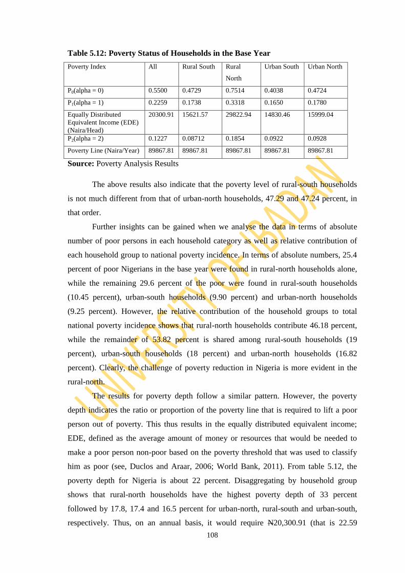
108

Table 5.12: Poverty Status of Households in the Base Year

Poverty Index All Rural South Rural

North

Urban South Urban North

P0(alpha = 0) 0.5500 0.4729 0.7514 0.4038 0.4724

P1(alpha = 1) 0.2259 0.1738 0.3318 0.1650 0.1780

Equally Distributed

Equivalent Income (EDE)

(Naira/Head)

20300.91 15621.57 29822.94 14830.46 15999.04

P2(alpha = 2) 0.1227 0.08712 0.1854 0.0922 0.0928

Poverty Line (Naira/Year) 89867.81 89867.81 89867.81 89867.81 89867.81

Source: Poverty Analysis Results

The above results also indicate that the poverty level of rural-south households

is not much different from that of urban-north households, 47.29 and 47.24 percent, in

that order.

Further insights can be gained when we analyse the data in terms of absolute

number of poor persons in each household category as well as relative contribution of

each household group to national poverty incidence. In terms of absolute numbers, 25.4

percent of poor Nigerians in the base year were found in rural-north households alone,

while the remaining 29.6 percent of the poor were found in rural-south households

(10.45 percent), urban-south households (9.90 percent) and urban-north households

(9.25 percent). However, the relative contribution of the household groups to total

national poverty incidence shows that rural-north households contribute 46.18 percent,

while the remainder of 53.82 percent is shared among rural-south households (19

percent), urban-south households (18 percent) and urban-north households (16.82

percent). Clearly, the challenge of poverty reduction in Nigeria is more evident in the

rural-north.

The results for poverty depth follow a similar pattern. However, the poverty

depth indicates the ratio or proportion of the poverty line that is required to lift a poor

person out of poverty. This thus results in the equally distributed equivalent income;

EDE, defined as the average amount of money or resources that would be needed to

make a poor person non-poor based on the poverty threshold that was used to classify

him as poor (see, Duclos and Araar, 2006; World Bank, 2011). From table 5.12, the

poverty depth for Nigeria is about 22 percent. Disaggregating by household group

shows that rural-north households have the highest poverty depth of 33 percent

followed by 17.8, 17.4 and 16.5 percent for urban-north, rural-south and urban-south,

respectively. Thus, on an annual basis, it would require N20,300.91 (that is 22.59

109

percent, which is the poverty gap, multiplied by N89867.81, which is the poverty line)

on average, to lift a poor person out of poverty nationally, while it requires N29,822.94,

N15,999.04, N15,621.57 and N14,830.46 to lift a poor person out of poverty in rural-

north, urban-north, rural-south and urban-south, accordingly. Clearly, fighting poverty

in the north would require more resources than combating poverty in the south.

Lastly, poverty is most severe within the rural-north households (18.54 percent)

and least severe among the rural-south households (8.71 percent). The severity of

poverty among urban-north and urban-south households is 9.28 and 9.22 percent

respectively. These results are further highlighted in figure 5.1 below:

Fig. 5.1 Poverty status of households in the base year

The results for poverty depth and severity perhaps underscore the need for other

measures apart from the headcount measure to be used in assessing poverty. For

example, in Nigeria, where the poverty headcount is over 50%, it may be practically

difficult to target all the poor at once, but with the poverty gap and squared poverty gap

measures, it is easier to target those whose poverty depth and severity is higher before

others or at least give them higher priority in the allocation of resources and poverty

interventions. Next, we discuss the impact of the various simulation experiments on the

poverty status of households in the base scenario.

110

5.6 Impact of Simulations on Poverty

In this section, the results of the impact of the scenario experiments on poverty

using the FGT class of poverty measures are presented and discussed. Second we

present the results and discussion by the type of shock across household groups and the

three FGT poverty measures. Finally, we compare the impacts of the shocks on

household groups by the poverty gap measure and the equally distributed equivalent

income. The poverty impacts are reported as percentage changes from the base levels

following a shock.

5.6.1 Impact of Food Price Shocks on Poverty

Table 5.13 shows the impact of food price shock on poverty, reported as

percentage change from the reference period. From the table, a 50 percent rise in the

world price of food imports increased the incidence of poverty nationally, and in all the

household categories albeit by varying degrees. National poverty headcount increased

by 3.254 percent. This increase in poverty headcount is as expected (since Nigeria is a

net food importer and is yet to be self-sufficient in food production), although the figure

is higher than 2.42 and 0.96 percent increase in poverty recorded by Boccanfuso and

Savard (2009) for Senegal and Mali, respectively as a result of a 70 percent increase in

the import price of food.

Rural-south households record the highest increase in poverty incidence of

almost 5 percent, followed by urban-north households, which registered a rise in

poverty headcount of a little above 4 percent. This shock increases the poverty

incidence of urban-south households by 3.86 percent, whereas rural-north households

experience the least increase in poverty headcount of 2 percent. It is worthy to notice

that the impact of this shock is higher for each household group than the national

average, except for rural-north households. These results are informative as they clearly

indicate that the impact of increased food prices was least felt by rural-north

households, perhaps due to the fact that the bulk of the staple food grains are produced

by the rural-north households. Thus, the increase in the price of food imports like rice,

maize, guinea corn, cowpeas, millet, etc, is not wont to affect rural-north households as

much as others. This suggests that this region could be harnessed to assure food security

in Nigeria.

The results also imply that although rural areas in Nigeria are mostly agrarian,

which preoccupation is subsistence production, food production in rural-south

111

households is poor as it negates this thesis, and hence the high impact of the shock on

this household category. Several reasons may account for this, which include quest for

formal education, penchant for engaging in commerce or trading (especially in the

south-east) instead of agriculture, poor agricultural conditions and output (especially in

Niger-Delta or south-south) due to oil spills and environmental degradation. For

example, a recent UNEP report indicates that it will take 30 years to clean-up oil spills

in the Niger-Delta region to make room for cultivating crops and revamping aquatic life

(see, The Guardian, 4 Aug, 2011).

For the poverty depth measure, we observe that rural-south and urban-north

households recorded the largest increase, with urban-north households recording the

highest increase in poverty gap of 6.5 percent, whereas rural-south poverty depth

increased by 6.2 percent. Urban-south and rural-north households record an increase of

5.3 and 4.2 percent respectively. These results are not surprising as the headcount

measure discussed above does not capture the extent to which individual income or

expenditure falls below the poverty line, the poverty depth measure, does. Jha and

Sharma (2003) have noted that certain policy changes or shocks favour one group of the

poor and adversely affect another group, and that in such cases, the headcount may not

register any change but the poverty gap index may get around it to some extent, thus the

need to use all three measures in analysis.

Table 5.13: Impact of Food Price Shock on Poverty (Percent)

Poverty Index All Rural South Rural North Urban South Urban North

P0(alpha = 0) 3.254 4.863 2.022 3.863 4.149

P1(alpha = 1) 0.579 6.271 4.219 5.394 6.504

P2(alpha = 2) 0.652 7.323 5.383 5.901 7.424

Source: Poverty Analysis Results

The results for poverty depth measure imply that it would require N20,823.78 on

average nationally to take a poor person out of poverty on an annual basis. If we

consider the quantum of resources required on the basis of households groupings, rural-

north households would require the greatest level of intervention; specifically, each

poor person in this household category would need N31,702.14 on average per year to

become non-poor. Urban-north households come next, requiring N17,381.33 on average

per person annually, to step out of poverty. This is then followed by rural-south

(N16,936.76) and urban-south (N15,940.84) households. This result implies that in

112

terms of targeting, rural-north households require more urgent attention than all other

households groups as far as this shock is concerned, in spite of the fact that it recorded

the lowest poverty incidence and the lowest increase in poverty gap. Clearly, the

poverty depth in the reference year based on the distribution for rural-north households

is very high, and hence the results.

In terms of poverty severity, urban-north households record an increase of 7.4

percent from the base, followed closely by rural-south households, with an increase of

7.3 percent from the base year. Also, rural-north households record the least increase in

poverty severity, as far as food price shocks are concerned. Figure 5.2 is a graphical

representation of the effect of this shock on the various household groups

Fig. 5.2 Impact of Food Price Shock on Poverty

5.6.2 Impacts of Oil Price shocks on Poverty

From the model simulation results in table 5.14, the impact of a fall in oil price

on households is mostly poverty-reducing. A 50 percent fall in the world price of oil

exports reduces the incidence of poverty nationally by approximately 1 percent. Urban-

north households experience the highest reduction in poverty incidence of 8.7 percent,

whereas rural-south households recorded the least reduction in the headcount measure

of 0.76 percent. Similarly, urban-south households experienced a 1.78 percent reduction

in poverty incidence. However, unlike other households, rural-north households actually

experienced an increase in poverty incidence of almost 3 percent, following this shock.

These results are quite plausible in terms of theory. According to Olomola and Adejemo

113

(2006), many studies have shown that rising oil prices reduced output and increased

inflation in the 1970s and early 1980s oil shocks, while falling oil prices boosted output

and lowered the general price (inflation). Also, Dorosh (1996), found that reductions in

the world price of oil hurt the poor less if real exchange rate was allowed to depreciate

than if foreign exchange restrictions prevented a real exchange rate adjustment. We

observe this pattern in the current study, as a 50 percent fall in oil price causes an

increase in sectoral output substantially and forces down domestic prices in all sectors

except manufactures/services.

In the Nigerian situation, this can further be explained from the government

expenditure point of view. This shock brings about fiscal austerity unlike an oil price

hike which earns the government windfall income. Thus, it is accompanied by reduced

government spending, which reduces the general price level, and so households

experience a reduction in the prices they face, which in the simulation were much lower

than the reduction in their incomes and consumption. Recall also that in the description

of the basic structure of the economy government spent over 64 percent of its income on

services and infrastructure and only about 3 percent on direct transfers to households.

Thus, a fall in government income would affect households more through public

consumption than transfers.

Table 5.14: Impact of Oil Price Shock on Poverty (Percent)

Poverty Index All Rural South Rural North Urban South Urban North

P0(alpha = 0) -1.127 -0.761 2.981 -1.783 -8.721

P1(alpha = 1) -1.328 -0.921 6.139 -1.679 -10.224

P2(alpha = 2) -1.508 -1.033 7.821 -1.844 -11.315

Source: Poverty Analysis Results

In terms of poverty depth and severity, a similar pattern like the one observed

for poverty incidence is observed for all households (see figure 5.3). Specifically, the

national poverty depth falls by 1.3 percent, whereas rural-south, urban-south and urban-

north record a reduction in poverty depth of 0.92, 1.67 and 10.22 percent, respectively.

Conversely, rural-north households experienced an increase in poverty depth of 6.14

percent. However, compared with the base scenario, it takes a lower amount of money,

on average, N19,637.72, nationally to lift a poor person out of poverty. Considering

each household category, rural-north, rural-south, urban-north and urban-south

households require N31,043.79, N15,186.45, N14,301.09 and N14,091.42, respectively

114

to lift a poor person out of poverty. Clearly, as far as this shock is concerned, rural-north

households need to be paid most attention in poverty alleviation efforts, followed

perhaps by rural-south households which experienced the lowest reduction in poverty.

Fig. 5.3. Impact of Oil price Shock on Poverty

5.6.3 Impacts of Exchange Rate shocks on Poverty

The impact of exchange rate depreciation in the model exacerbates national and

household poverty; the extent of which depended greatly on the consumption (of local

or imported goods) and production (for domestic or export market) patterns of the

households and to some extent the proportion of their income that is obtained from

foreign transfers. Table 5.15 points out that this shock increased national poverty

incidence by about 1.7 percent. Urban-north households suffer the highest increase in

poverty headcount of 3.3 percent, while rural-north households suffer the least impact,

with less than 0.5 percent increase in poverty incidence. Rural-south and urban-south

households experience an increase of about 2.5 and 2 percent in poverty headcount,

respectively. These results may imply that urban-north households are the largest

culprits in the consumption of imported products. Although the results indicate that

rural-south households come next in terms of poverty incidence, it may be that they are

implicated more than urban-south households because the latter might have been

exporting a good quantity of products as they consume imports, compared with rural-

south households. For rural-north households which are the least affected by this shock,

it may be that they consumed less of imported commodities while they produced much

115

in terms of primary agricultural commodities that may likely be import substitutes, for

example, rice, maize, sorghum, wheat, livestock, etc.

Table 5.15: Impact of Exchange Rate Shock on Poverty (Percent)

Poverty Index All Rural South Rural North Urban South Urban North

P0(alpha = 0) 1.696 2.529 0.331 2.172 3.315

P1(alpha = 1) 2.651 3.164 0.690 2.562 5.494

P2(alpha = 2) 3.154 3.670 0.895 2.755 6.250

Source: Poverty Analysis Results

These results make sense even further when the proportion of total expenditure

of households‘ expenditure on items that are most likely to be imported (namely

beverages, processed food, textiles, furniture, transport/other equipment, other

manufactures) is compared among the households groups. It is interesting to see that

17.5 percent of urban-north households‘ expenditure went to imported products,

compared with 12.8 percent from urban-south. Rural-north households spent the least

(9.3 percent) on imported commodities, whereas rural-south households took the second

position (13.7 percent) as indicated by the simulation results.

The results for changes in poverty depth and severity in the table show a similar

pattern (see Fig. 5.4). Nationally, the poverty depth increased by 2.65 percent. Among

the household categories, urban-north households experienced the highest increase in

the depth of poverty of 5.5 percent followed by 3.2 percent for rural-south households,

2.6 percent for urban-south households and lastly, 0.7 percent for rural-north

households. This same order is repeated for poverty severity: 3.15 percent nationally,

and 6.25, 3.67, 3.15 and 0.89 correspondingly for urban-north, rural-south, urban-south

and rural-north households.

However, rural-north households need more money (N35,378.605) on average

for a person to be taken out of poverty compared with the national average

(N24,555.57) and urban-north households (N19,885.15), which experienced the highest

impact of exchange rate depreciation. The least effort to lift individuals out of poverty is

required in urban-south households (N17,920.12) after households in the rural-south

category (N18,989.01). These results draw attention to the importance of the poverty

gap measure, even though this shock did not affect rural-north households as much as

the others, this measure still indicates that that household group needs the most help as

far as this shock is concerned.

116

Fig. 5.4. Impact of Exchange Rate Shock on Poverty

5.6.4 Impacts of All shocks Combined Poverty

The last simulation, which combines the first three scenarios, has a remarkable

effect on poverty with some interesting results. The resulting direction and perhaps, the

magnitude of the effects underscore the overarching impact of some external shocks on

household poverty and distributional outcomes. They further highlight the conception

advanced earlier in section two, that the impact of positive shocks are easily over-

swamped by those of negative ones, especially when they occur simultaneously. Of the

three macroeconomic shocks explored in this study, increase in food prices and

exchange rate depreciation caused a worsening of household poverty while a fall in oil

price was, in the main, poverty-reducing. However, the combined scenario clearly

showed that the impact of the three shocks, which occasioned the global economic

crisis, taken together, exacerbated poverty in Nigeria, with some appealing implications.

From the macro results, this simulation led to a fall in household

incomes/expenditures except those of urban-north households. Domestic output

increased (except for the crude oil due to depressed export price). Imports volume

dropped remarkably, while there was an increase in exports except crude oil exports for

the same reason stated earlier. Prices of domestic output dropped except in

manufactures/services. Overall, household income had fallen more than domestic prices

thus leading to a rise in the poverty line as earlier noted. Thus, under this scenario, as

shown in table 5.15, national poverty incidence increased by about 5.7 percent, while

increase in household poverty showed rural-south households recording an 8.56 percent

117

increase, followed by rural-north and urban-south households, with roughly a 7 percent

increase poverty headcount each. However, there was no change in the poverty

incidence of urban-north households as a result of this combined shock. As far as the

headcount measure is concerned, rural-south households were the worst hit by the

global economic meltdown as it affected Nigeria, whereas, urban-north households

were not affected at all, considering the combined effects of the shocks. This is

intuitively appealing in that, the urban-north households experienced the highest

reduction in poverty as a result of the oil price shock, and it was only possible for the

effect of the other two shocks to knock off that gain, without aggravating their poverty

status.

Table 5.16: Impact of All Shocks Combined on Poverty (Percent)

Poverty Index All Rural South Rural North Urban South Urban North

P0(alpha = 0) 5.727 8.562 7.061 6.922 0.000

P1(alpha = 1) 8.490 11.064 14.578 8.315 0.617

P2(alpha = 2) 10.130 12.913 18.964 9.11 0.743

Source: Poverty Analysis Results

However, in terms of poverty depth measure, rural-north households recorded

the deepest plunge into poverty of about 14.5 percent, whereas rural-south and urban-

south households went deeper by 11 and about 8.5 percent, respectively. Urban-north

households only showed a marginal increase of less than 1 percent in poverty depth.

This is not surprising as the poverty gap measure is able to highlight an important aspect

of poverty that is usually masked by the headcount measure. Under this scenario, it

takes an average of N22,840.361 nationally to make an individual non-poor per annum.

This is actually higher than the amount needed to take an individual out of poverty in

rural-south (N17,989.89), urban-south(N16,656.41) and urban-north (N16,689.609)

households, while it is much lower than the N35,429.87 that it takes to lift a poor

person out of poverty in rural-north households, per annum on average. This implies

that the task of reducing the poverty gap would be greatest in rural-north households.

Further results indicate that poverty severity increased by about 10 percent

nationally. Breaking this down by household groups, rural-north households recorded

the highest increase in poverty severity from base level, of almost 19 percent, followed

by almost 13 percent experienced by rural-south households. Urban-south households

recorded an increase in poverty severity of 9 percent, whereas the least increase in

118

poverty severity of 0.74 was recorded by urban-north households. One striking feature

of rural-north households is that in all the simulations, including one that reduced

poverty in other household groups, their poverty situation based on all the measures,

worsened. Figure 5.4 depicts the response of the households‘ poverty to this simulation.

Fig. 5.5 Impact of the Combined Shock on Poverty

On the whole, the simulations experiments indicate that while food price shocks

and exchange rate shocks increased poverty, falling oil price shocks were mostly

poverty-reducing (this result makes sense in that, as indicated earlier, rise in oil prices

may lead to an increase in the general price level which then reduces consumers

purchasing power thus exacerbating poverty and vice versa). But the combine effects of

the three shocks indicate an increase in poverty, as implicated by the effects of

exchange rate and food price shocks. These results have dire implications for policy.

5.6.5 Comparison of the Impacts of Simulations on Household Groups by

Poverty Gap Measure and Equally Distributed Equivalent Income

Table 5.16 shows the poverty depth impact of the simulations alongside the

equally distributed equivalent income (EDE), which shows the average amount of

money required to bring a poor person out of poverty; in other words, the average

distance between the income of each of the household members and the poverty line.

Figure 5.5 on the other hand is a graphical representation of the EDE income. From the

119

table, we fine that even where the change in poverty gap registered by other households

is higher for a given simulation than in rural-north households, this household group

still registers the highest EDE income. This implies that there was widespread poverty

in the original distribution of incomes/expenditure of this household group compared

with the others. The graph indicates that the resources required tackling poverty in

rural-north households are almost double those required by the other household

categories in almost all the scenarios.

Table 5.17 Poverty Gap Impact and Equally Distributed Equivalent Income of

Household Groups

All Rural

South

Rural North Urban

South

Urban

North

Food

Price

P1 0.579 6.271 4.219 5.394 6.504

EDE (Naira) 20832.78 16936.76 31702.14 15940.84 17381.30

Oil Price P1 -1.328 -0.921 6.139 -1.679 -10.224

EDE (Naira) 19637.72 15186.45 31043.79 14091.42 14301.09

Exc. Rate P1 2.651 3.164 0.690 2.562 5.494

EDE (Naira) 24555.57 18989.01 35378.605 17920.12 19885.15

All P1 8.490 11.064 14.578 8.315 0.617

EDE (Naira) 22840.36 17989.89 35429.87 16656.41 16689.609

Source: Poverty Analysis Results

0

5000

10000

15000

20000

25000

30000

35000

40000

All Rural-South Rural-North Urban-South Urban-North

EDE1

EDE2

EDE3

EDE4

Fig. 5.6: Equally Distributed Equivalent Income by Household Groups Following the

Shocks

5.7 Impact of Simulations on Income Inequality

In this section we present and discuss the results of the analysis of the impact of the

shocks on income inequality nationally and at the socioeconomic group level in the base

year, followed by the post-shock impacts at the national level for all shocks. This

120

analysis is important because inequalities in income distribution, access to productive

resources and basic social services have been cited as causing and exacerbating poverty

(see, for instance, Naschold, 2002; United Nations, 2005).

In the base year, national Gini coefficient is 0.4176 (table 5.18). This implies that

the average distance between the incomes of the households in the distribution is in the

order of 83.52%. Put in terms of difference in income, the value represents the expected

difference in incomes of two individuals or households randomly selected from the

population as a whole. Looking at the household groupings, we find that urban-north

households have the highest Gini coefficient of 0.422, followed by urban-south

households, with an index of 0.4197. Rural-north households record the least inequality

(0.3637) in their income distribution, before rural-south households with a Gini index of

0.3781. It can be noticed that inequality is higher among urban households than among

their rural counterparts. This implies the extent of relative deprivation is higher in urban

areas than in rural areas, which quite in line with literature (see, Aredo, Fekadu, and

Workneh, 2008).

Table 5.18: Inequality Levels in the Base Year

Gini Index All Rural South Rural North Urban South Urban North

Base 0.4176 0.3781 0.3637 0.4197 0.4244

Source: Inequality Analysis Results

Table 5.19 shows the impact of the simulation experiments on inequality. From the

table although slightly, food price shocks and exchange rate shocks reduced inequality

nationally by 0.0478 and 0.2586 percent, respectively, whereas oil price shocks

increased inequality, by about 1.4 percent. This may be due to the fact that the changes

in relative prices following food price and exchange rate shocks shift resources in

favour of the poor segment of the income distributions; however, since oil price shocks

do not have direct effects on the prices faced by these households, the impact tends to

worsen inequality. These results show that poverty can decrease even when inequality is

rising.

It can be observed that the magnitudes of the inequality changes are quite small

when compared to the magnitude of the simulations. This is common in CGE literature,

as they have been known to produce small distributional impacts (see, Nwafor et al,

2005; Adenikinju and Falobi, 2006; Annabi, Cisse, Cockburn and Decaluwe, 2007).

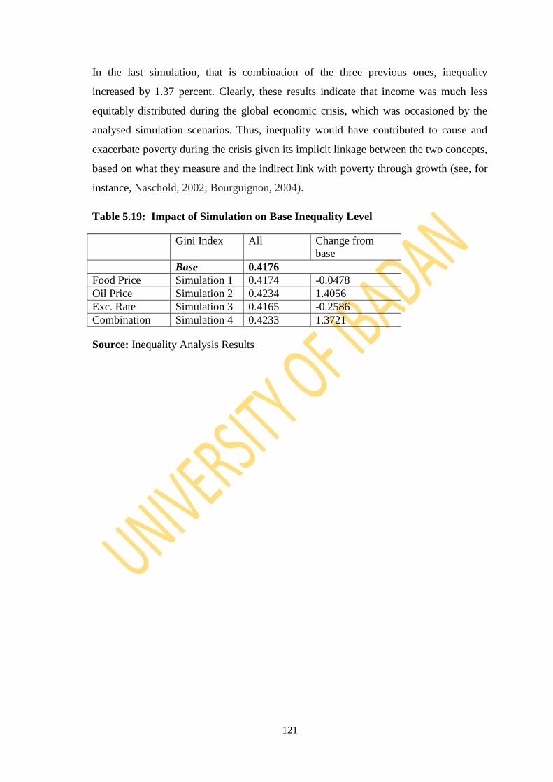
121

In the last simulation, that is combination of the three previous ones, inequality

increased by 1.37 percent. Clearly, these results indicate that income was much less

equitably distributed during the global economic crisis, which was occasioned by the

analysed simulation scenarios. Thus, inequality would have contributed to cause and

exacerbate poverty during the crisis given its implicit linkage between the two concepts,

based on what they measure and the indirect link with poverty through growth (see, for

instance, Naschold, 2002; Bourguignon, 2004).

Table 5.19: Impact of Simulation on Base Inequality Level

Gini Index All Change from

base

Base 0.4176

Food Price Simulation 1 0.4174 -0.0478

Oil Price Simulation 2 0.4234 1.4056

Exc. Rate Simulation 3 0.4165 -0.2586

Combination Simulation 4 0.4233 1.3721

Source: Inequality Analysis Results

122

CHAPTER SIX

SUMMARY, CONCLUSIONS AND RECOMMENDATIONS

6.1 Introduction

This study examined the impact of macroeconomic shocks on household poverty

and income inequality in Nigeria, motivated by the recent global economic crisis.

Specifically, the study investigated the impact of three different shocks, namely food

price shock, oil price shock and exchange rate shock as well as their combination,

experienced in Nigeria in the wake of the economic crisis, on household poverty and

income inequality.

Secondary data, collected in the main, from the National Bureau of Statistics (NBS)

and the International Food Policy Research Institute (IFPRI) were relied upon in

meeting the specific objectives and arriving at the results of the study. The data were

analysed using a macro-micro framework, which comprised a computable general

equilibrium model (which provided the economy-wide general equilibrium results on

changes in prices, households‘ incomes and demand) and a module that involved

poverty and inequality measurement, using the FGT and Gini indexes, respectively. The

summary of major findings of the study is subsequently discussed.

6.2 Summary of Major Findings

Beginning with the descriptive of the structure of the Nigerian economy in the base

year, we find that the average incomes of incomes of rural households are very low.

Precisely, the estimated average income of rural-south and rural-north households were

N85,421.051 and N77,062.578 per person per annum, respectively. These translate into

N234.03 (or US$1.56) and N211.13 (or US$1.41) per day for rural-south and rural-

north households accordingly, which are less than all the endogenous poverty lines used

in the study and also less than the recommended minimum income of US$2 per day for

most developing countries by the World Bank (2008).

Another key finding in this section hinges on the consumption pattern of the

households in Nigeria. Rural households spent over 61 percent of their income on food,

while urban household spent between 54 and 62 percent of their incomes on

manufactures/services. Furthermore, the share of imports in total household

consumption was roughly 39 percent, which calls for serious concern. Of this

proportion, about 6 percent of households‘ consumption of food was accounted for by

123

imports, while the share of imports consumed in other agriculture and

manufactures/services stood at approximately 26 and 76 percent, respectively.

In the reference year, we find that poverty incidence was already very endemic in

Nigeria and among the four household groups considered in the study. Thus, before the

shocks, 55 percent of Nigerians were poor in terms of headcount, while the incidence of

poverty in rural-north, rural-south, urban-north and urban-south households stood at 75,

47, 47 and 40 percent, respectively. These results indicate that rural-north households

were the poorest socioeconomic group in the country and also that the poverty status of

rural-south and urban-north household was the same. One interesting feature of this

finding is that in terms of absolute numbers, 25.4 percent of poor Nigerians in the base

year were found in rural-north households alone, while the remaining 29.6 percent of

the poor were in the other household groups, taken together. Thus, in relative terms,

rural-north households alone accounted for about 46 percent of poverty in Nigeria.

The food price shock increased poverty nationally and among all the households. A

50 percent increase in the price of food imports increased poverty in rural-south

households by 5 percent followed by a 4 and 3.8 percent increase in poverty of urban-

north and urban-south households, in that order. Rural-north households were the least

affected by this shock as their poverty incidence increased by just 2 percent.

The impact of the oil price shock was mostly poverty-reducing. From the model

simulation results, a 50 percent fall in export price of crude oil led to an 8.7 percent

reduction in poverty incidence of urban-north households, followed by a 1.78 and 0.76

percent reduction in the headcount measure of poverty in rural-south and urban-south

households respectively. However, a fall in the price of crude failed to reduce poverty in

rural-north households, but actually increased poverty in this socioeconomic group by

almost 3 percent.

The impact of exchange rate depreciation aggravated the poverty situation across

board with substantial effects on all household categories. The individual effects on all

but one household group were higher than the national average impact. A 25 percent

increase in the exchange rate increased national poverty incidence by about 1.7 percent.

Urban-north households suffered the highest increase in poverty headcount of 3.3

percent, while rural-north households suffered the least impact, with less than 0.5

percent increase in poverty incidence. Rural-south and urban-south households

experienced an increase of about 2.5 and 2 percent in poverty headcount, respectively.

124

The results of the combination scenario were quite remarkable, as they actually

produced the strongest impacts that we have seen in this study. Thus, under this

scenario, we found an increase in national poverty incidence of about 5.7 percent.

Regarding the household categories, rural-south household‘s poverty situation worsened

the most as they recorded an 8.56 percent increase, followed by rural-north and urban-

south households, with roughly a 7 percent increase poverty headcount each.

Interestingly, however, there was no change in the poverty incidence of urban-north

households as a result of this combined shock. These results are very informative as we

find that in combination, the negative impacts of food price and exchange rate shocks

over-swamped the poverty-reducing effect of oil price shocks and even worsened the

poverty situation of all the household groups except one (urban-north households),

which situation in terms of poverty incidence did not change.

One finding that need be viewed seriously as far as this study is concerned is the

impact of the poverty gap measure and the equally distributed equivalent (EDE)

incomes, as it provides a depiction of what the amount of resources that would be

required to move all poor people to the poverty threshold. We find that for the

combination scenario (which mirrors the crisis period), the equally distributed

equivalent income nationally was N22,840.36, implying that on average, at the national

level, if each poor individual receives N22,840.36, they would become non-poor based

on the endogenous poverty lines used in this study. But even more informative is that of

the four household categories, three, namely, rural-south (N17,989.89), urban-south

(N16,656.41) and urban-north (16689.609) households have EDE incomes that are

lower than the national average while rural-north households have the highest EDE

income of N35,429.87. This trend was observed across all the simulations. Thus, we

find that in reducing poverty in Nigeria, rural-north households would require almost

twice as much resource as would be needed to tackle poverty in any of the other three

household groups.

Finally, in the base year, we find that inequality was higher in urban households

(0.4197 for urban-south and 0.4244for urban-north) than in rural households (0.3781 for

rural-south and 0.3637 for rural-north), and that urban household inequality levels were

higher than the national inequality index (0.4176). The impact of the simulations on

inequality for the individual shocks were rather mixed in the sense that although

marginally, food price and exchange rate shocks potentially reduced inequality by

0.0478 and 0.2586 percent, respectively, oil price shock increased inequality, by about

125

1.4 percent, which was quite in contrast to their effects on poverty. However, the

expected picture showed up in the combination scenario, as inequality increased by 1.37

percent, in line with poverty increases in the poverty analysis of the impact of this

simulation. These results show that poverty can decrease even when inequality is rising.

6.3 Conclusions

This study investigated the impact of macroeconomic shocks on household poverty

and income inequality in Nigeria. Based on the results, the study has shown that the

global economic crisis occasioned by the simulated shocks impacted the Nigerian

economy and households in Nigeria negatively (as national poverty incidence increased

by 5.7 percent and even by a higher proportion in rural-south (8.56 percent), and 7

percent in rural-north and urban-south households), thus affirming the notion that the

country is not insulated to external shocks. The magnitude and direction of the impact,

however, varied by individual shocks and household groups, but importantly, increases

in food price as well as increase in the naira/dollar exchange rate were the major

perpetrators of the negative impacts on poverty, as they increased national poverty by

3.25 and 1.7 percent, respectively, while they turned out to show potential for reducing

inequality, as they reduced national inequality levels by 0.048 and 0.26 percent

respectively. In contrast, fall in oil price mostly reduced poverty (nationally by 1.13

percent), while at the same time exacerbated inequality by about 1.41 percent.

Consequent upon the above results, we assert that there could be an increase in

poverty even when inequality remains unchanged or falls marginally, especially if the

reduction in incomes is even across households. This seems to be in conflict with the

thesis that poverty and inequality reinforce each other (McKay, 2002; Naschold, 2002),

as we found that it may not apply in all cases. The impact of oil price on poverty and

inequality further negates the notion about the acclaimed implicit relationship between

poverty and inequality, as stated earlier, and leads us to the conclusion that shocks that

may reduce poverty may not necessarily be egalitarian in their impact, thus calling for

attention to be paid to the fact that pursuing poverty reduction policies with the implied

aim of tackling both poverty and inequality may actually worsen income distributions

and vice versa.

One new insight gained from this study is that shocks which have the potential of

increasing poverty but redistributing wealth are those whose effect are mostly direct, for

example, food price and exchange rate shocks, transmitted through income,

126

employment and price changes, while those that might have the opposite effect of

reducing poverty but worsening income distribution belong to the group which effects

might be basically indirect, for example, oil price shock in the Nigerian situation, which

major transmission channel is via government fiscal stance through its spending, before

affecting prices.

Another important lesson from this study is that overall, when all the shocks were

allowed to act simultaneously, the resulting impact was negative: poverty increased and

inequality also worsened. This conforms to the theory that inequality is bad for or fuels

poverty (see, Killick, 2002). However, some of the results in this study have indicated

that it may not always be so, unless perhaps when both direct and indirect mechanisms

act together. Thus, we conclude on this score that the relationship between poverty and

inequality can be very fluid, both in terms of signal and causality.

Another important conclusion drawn from the study is that the impact of shocks

would depend more on the economic fundamentals of the nation and its households or

socioeconomic groups than on policy response mechanisms to such shocks, based on

the recurring strong impacts of the shocks on rural-north households, which in the study

had the worst poverty status in the reference year and which required the most

intervention after the shocks than any other household group. This household group has

shown how strong the negative impact of shocks can be when the initial economic

structure was poor. It has also shown how the impact of some shocks can be minimal

depending on the households‘ income sources and consumption structure in the sense,

for example that it was the least affected in terms of headcount measure, by food price

shock for reasons perhaps of producing more food than other household groups and

consuming less of imported food and manufactures/services.

6.4 Policy Recommendations

Although poverty reduction and income equity issues require actions on broad

fronts, the results of the study point to some specific implications that require specific

interventions, which may be targeted at some socioeconomic groups, as well as broad-

based policy actions, which might necessarily have a national outlook. An important

message from the current analysis is that the initial economic structure or fundamentals

determine, to a great extent, the impact of the various shocks on the various sectors as

well as household groups in the model. Thus, the recommendations proffered here to

127

guide or inform public policy interventions implicitly address this concern amongst the

implication(s) that arise from the simulation experiments.

A. Food Price Shock: The results have shown that households, particularly rural

households spend a substantial portion of their incomes on food, which means

that an increase in the price of food would lower their real income, reduce their

consumption and hence welfare. This therefore suggests that if abundant or more

food is produced, to the extent that we would no longer have to rely much on

imported food, any increase in the price of imported food would have very

minimal impact on the price of food that is produced and sold domestically.

Furthermore, the impact of food price shock was least in rural-north households,

and as was stated earlier, a plausible explanation could be that they relied much

less on imported grains as they produce a good quantity of grains. Thus it is

recommended that:

i. In the long-term, boosting food production especially in rural-south

households and stepping up same in rural-north households is key, as

increased agricultural productivity in rural areas would assure availability of

affordable food and enhance the already very low per capita rural incomes.

ii. In the short-term, however, palliative measures, as response to food price

increase would, include measures to bring down food price and/or measures

that can increase the purchasing power of households. For the first

intervention strategy, staple food grains can be released from strategic

reserves into the markets in the rural-south, particularly, as well as other

regions most affected by the shock. Safety-net programmes, such as school

feeding in the most affected areas are another short-term measure.

B. Oil Price Shock: As it concerns oil price shock, the study recommends that:

i. In the interim, hedging against future price volatility can help in

reducing the impact of world oil price shocks on the Nigerian economy.

Another short-term recommendation is that rural-north households that

have suffered the most impact from the shock should be directly targeted

with safety-net programmes like food-based programmes to help in

cushioning the adverse effect of the shock.

ii. In the long-run, diversification of the economy through investments in

production sectors using oil windfall incomes and developing alternative

128

sources of government revenue will reduce over-dependence on oil

revenue, as well as the impact of its price shock on the economy.

C. Exchange Rate Shock: Since the impact of exchange rate shock is mostly felt

by households through the goods they consume and/or produce and we found in

the study that the import of manufactured goods (which include processed foods

like dairy product, canned meat/fish, sugar, beverages, etc) had the highest

proportion in the list of imports. It is therefore important to change the

production and trade structure of the economy. Thus it is recommended that:

i. An effective and efficient infrastructural system that supports

manufacturing, agro-processing and efficient service delivery should be

pursued so that foreign companies that use raw materials from Nigeria

can be encouraged to open factories and manufacture those good here in

the country, as this would have a broad impact of reducing the adverse

effect of exchange rate shocks on households that consume imported

products.

ii. Moreover, diversification of the export base and export promotion as

well as import-substitution is crucial. Agricultural exports should be

boosted by encouraging the production of say, cassava for export by

rural-south households. But in the case of northern households, the

poverty impact of exchange rate shocks can be reduced by providing an

incentive for the unskilled and low education urban-north households

who constitute the bulk of the urban poor to migrate back to the rural-

north areas by developing the rural-north areas in terms of infrastructure.

This is bearing in mind that the rural-north households were the least

affected by this shock.

iii. In the long-term, apart from, interventions to change the production and

trade structure in terms of broad-based diversification of production to

include import substitutes and the promotion of exports, proper

management of the external reserves is important. It is recommended that

increasing the external reserves when there is economic boom can help

stabilized the exchange rate during economic busts.

D. On the issue of inequality, it is recommended that both broad-based and targeted

interventions be pursued in the areas of education, healthcare, improving social

capital, as well as, expanding and improving access to basic infrastructural

129

services. One way of achieving this would be taxing the richer segment of

society, which is a means of ensuring income redistribution and equity.

6.5 Limitations of the Study and Suggestions for Further Research

As in any empirical research endeavour, this study has its limitations, stemming

mainly from data and model development issues rather than the question that was

investigated. The data requirements of CGE models are very demanding, thus to

capture the nuances in the behaviour of the economy, sectors and agents requires

highly detailed databases, which in most cases are lacking in developing countries,

especially given that the data sources for assembling the database (or SAM) are very

numerous. Consequently, since the equations of CGE model derive from the SAM

underlying the state of the economy which is being modelled at equilibrium, it

follows that the SAM would determine the working of the model. Beyond this,

carrying out poverty analysis in a general equilibrium framework has its added data

as well as modelling challenges. As it concerns the data, it is difficult for the SAM

and household survey data to both be available for the same year at the time of

analysis. Thus, aside the inherent shortcomings of the household surveys

themselves, the assumption that the economic structure does not change

significantly within a band of a certain number of years may not hold, as results

might be affected by structural changes. Consequently, the following suggestions

are made for future research.

(i) Future studies on poverty analysis using the current representative household

CGE approach should use a different classification of household groups

based along the lines of not just geographic locations but also along

occupational and educational dimensions. This way some more detailed

effects can be observed that might help policy actions to be more focussed,

given that the dimensions of poverty are quite diverse. This of course

depends on the availability of a detailed and consistent household survey and

SAM data.

(ii) Since the simulations in the current study were carried out in comparative

static mode, the dynamic effects of the simulations were not captured,

although some analysts argue that the manner in which the CGE model is

closed might indicate whether the results should be interpreted as short- or

130

long-run impacts. Thus, there is need for further studies to model dynamics

so as to predict the steady-state and dynamic growth path of the shocks.

(iii) Future research should also be carried on the basis of CGE micro-

simulation analysis which is more complex in terms of computational

demands, using all the households in a survey and fed into the CGE model

through a micro-simulation module in order to capture the intra-group

variances which are ignored in the current representative household model.

This way the analysis of both poverty and inequality for each household in

the survey rather than household group can be carried out.

131

REFERENCES

Abdelkrim, A. and Awoyemi, T. T. (2006). Poverty and Inequality Nexus: Illustrations

with Nigerian Data. Cahier de recherche/Working Paper 06-38

Acemoglu, D., Johnson, S., Robinson, J., and Thaichareon, Y. (2003). Institutional

causes, macroeconomic symptoms, volatility, crisis and growth. Journal of

Monetary Economics, 50: 49-123.

Adamu, A. (2009). The Effects of Global Financial Crisis on Nigerian Economy.

Mimeograph, Department of Business Administration, Nasarawa State

University, Keffi

Adenikinju, A., Ajakaiye, O., Decaluwe, B. and Iwayemi, A. (Eds.) (2009). Computable

General Equilibrium Modelling in Nigeria. Ibadan: Ibadan University Press

Adenikinju, A. F. and Falobi, N. (2006). Macroeconomic and Distributional

Consequences of Energy Supply Shocks. Research Paper 162, African

Economic Research Consortium, Nairobi, Kenya

Addison, T. and Cornia, G. A. (2001). Income Distribution policies for Faster Poverty

Reduction. UNU-WIDER Discussion Paper No. 93, Helsinki, Finland

Ahmed, S. (2003). Sources of macroeconomic fluctuations in Latin America and

implications for choice of exchange rate regime. Journal of Development

Economics, 72: 181-202

Agenor, P. R. and Montiel, P. J. (1999). Development macroeconomics, (2nd

ed.).

Princeton: Princeton University Press

Agenor, P. R. (2005). The Macroeconomics of Poverty reduction. The Manchester

School, 73(4), 369-434

Aigbokhan, B. E. (2008). Growth, Inequality and Poverty in Nigeria. ACGS/MPAMS

Discussion Paper No. 3,United Nations Economic Commission for Africa

(UNECA), Addis Ababa.

Ajakaiye, D. O. and Adeyeye, V. A. (2002). Concepts, Measurement and Causes of

Poverty. Central Bank of Nigeria Economic and Financial Review, 39(4):

Alesina, A. and Perotti, R. (1993). Income Distribution, Politicial Instability and

Investment. NBER Working Paper No 4486.

Aliu, A. (2001), National Poverty Eradication Programme (NAPEP): Completion,

Implementation, Coordination and Monitoring, NAPEP Secretariat, Abuja,

April.

132

Aliyu, S. U. R. (2009). Impact of oil price shock and exchange rate volatility on

economic growth in Nigeria: An Empirical Investigation. Munich Personal

RePEc Archive Paper No. 16319. Retrieved 22 February 2011 from

http://mpra.ub.uni-muenchen.de

Altimir, O. and Beccaria (2002). Efectos de Cambios Macroeconomicos y de Reformas

sobre La Pobreza Urbanaen Argentina. Banco Interamicano de Desarrollo,

Departmento de Desarrollo Sostenible. Washington DC

Aka, B. F. (2006). Poverty, Inequality and Welfare Effects of Trade Liberalization in

Côte d'Ivoire: A computable General Equilibrium Model Analysis. Research

Paper 160 African Economic Research Consortium, Nairobi, Kenya

Akpan, E. O. (2009). Oil Price Shocks and Nigeria‘s Macroeconomy. Retrieved 15

August 2011 from www.csae.ox.ac.uk/conferences/2009-EDiA/papers/252-

Akpan.pdf

Amis, P. and Rakodi, C. (1994). Urban Poverty: Issues for research and policy. Journal

of International Development, 6(5): 627 – 34

Annabi, N., Cisse, F., Cockburn, J. and Decaluwe, B. (2007). Trade Liberalization,

Growth and Poverty in Senegal: A Dynamic Micro-simulation CGE Model

Analysis. CEPII, Working Paper No. 2005-07

Annabi, N., Cisse, F., Cockburn, J. and Decaluwe, B. (2009). Functional Forms and

Parameterization of CGE Models, In: Computable General Equilibrium

Modelling in Nigeria (Ed): Adenikinju, A. F., Ajakaiye, O. and Iwayemi, A.

(2009). Ibadan: University of Ibadan Press

Anyanwu, J. C. (1997). Poverty in Nigeria: Concepts and Measurements and

Determinants In: Poverty Alleviation in Nigeria, Selected Papers, Nigeria

Economic Society Annual Conference

Aredo, D., Fekadu, B. and Workneh, S. (2008). Trade Liberalization, Poverty and

Inequality in Ethiopia: A CGE Analysis. Working Paper, Poverty and Economic

Policy (PEP) Research Network

Armington, P. (1969). A Theory of Demand for Products Distinguished by Place of

Production. IMF Staff Papers, 16: 159-176.

Arrow K. J. and G. Debreu (1954). The Existence of an Equilibrium for a Competitive

Economy, Econometrica, 27, 265-90

133

Asian Development Bank (2011). Poverty Definition, Measurement, and Analysis.

Retrieved 19 July 2011 from www.adb.org/Documents/Handbooks/Analysis -

Processes/appendix01.pdf

Atkinson, A. (1997). Bringing Income Distribution in from the Cold. Economic Journal

107, 297-321.

Atkinson, A. B. (1998). Poverty in Europe. Oxford: Basil Blackwell.

Bautista, R. and Thomas, M. (1997) Income Effects of Alternative Trade Policy

Adjustments on Philippine Rural Households: A General Equilibrium Analysis.

TMD Discussion Paper No. 22, International Food Policy Research Institute.

Bellu, L. G. and Liberati, P. (2006). Policy Impacts on inequality: Inequality and

axioms for its measurement. Rome: Food and Agriculture Organisation of the

United Nations

Benjamin, N. (1996). Adjustment and Income Distribution in an Agricultural Economy:

A General Equilibrium Analysis of Cameroon. World Development, 24(6):

1003-1013

Bhasin, V. K and Annim, S. K. (2005). Impact of Elimination of Trade Taxes on

Poverty and Income Distributions in Ghana. Revised Final Report Submitted to

Global Development Network (GDN)

Bhasin, V. K and Obeng, C. K. (2004). Trade Liberalization, Foreign Borrowing,

Poverty and Income Distribution of Households in Ghana.

www.ecomod.net/conferences/ecomod2005/ecomod2005_Papers/623.doc

Bhasin, V. K. and Obeng, C. K. (2005). Trade Liberalization, Remittances, Poverty and

Income Distributions of Households in Ghana. A Paper Submitted for the

Econometric Modelling Conference, May.

Birdsall, N., Ross, D., and Sabot, R. (1995). Inequality and Growth Reconsidered:

Lessons from East Asia. World Bank Economic Review 9, 477-508.

Birdsall, N. and Londono, J. (1997). Asset Inequality Does Matter: Lessons from Latin

America. Washington, D.C.: Inter America Development Bank.

Black, F. (1995). Exploring General Equilibrium. Cambridge Massachusetts: MIT

Press.

Blackwood, D. L. and Lynch, R. G. (1994). The measurement of Inequality and

Poverty: A Policy maker‘s guide to the Literature. World Development, 22(4):

567-68

134

Boccanfuso, D., Decaluwe, B. and Savard, L. (2003). Poverty, income distribution and

CGE modelling: Does the functional form of the distribution matter? Cahier de

recherché/Working Paper 03-32 CIRPEE

Boccanfuso, D. and Savard, L. (2005). Impact Analysis of the Liberalization of

Groundnut Production in Senegal: A Multiple Household CGE Model. Cashiers

de recherché/Working Paper 05/12, Groupe de Recherche en Economie et

Developpment International, GREDI

Boccanfuso, D. and Savard, L. (2009). The Food Crisis and its Impacts on Poverty in

Senegal and Mali: Crossed Destinies. Cashiers de recherché 08-20, Department

d‟Economique de las faculte d‟administration „a l‟universite de Sherbrooke.

Bonnet, C, and Mahieu, R. (2000). Public Pensions in a Dynamic Micro-analytic

Framework: The Case of France: In Mitton, L., Sutherland, H. and Weeks, M.,

Micro-simulation Modelling for Policy Analysis: Challenges and Innovations,

Cambridge: Cambridge University Press.

Bourguignon, F., Robillard, A.-S., and Robinson, S. (2002). Representative versus Real

Households in the Macro-economic Modelling of Inequality, Mimeograph.

Washington DC: World Bank.

Bourguignon, F. (2004). The Poverty-Growth-Inequality Triangle. Paper presented at

the Indian Council for Research on International Economic Relations, New

Delhi: February

Bruno, M., Ravallion, M. and Squire, L. (1996). Equity and Growth in Developing

Countries: Old and New Perspectives on the Policy Issues. Washington, D.C.:

World Bank.

Busari, D. T. and Udeaja, E. A. (2007). Tariff and Factor Allocation in a Small Open

Economy: Nigeria. Economic and Financial Review, Central Bank of Nigeria,

45(2): 73-98

Busari, D. T. (2009). Economic Reforms and Deforestation: Policy Simulations for

Nigeria. In: A. Adenikinju, O.Ajakaiye, and A. Iwayemi (Eds.), Computable

General Equilibrium Modelling in Nigeria (pp.227-250). Ibadan: University of

Ibadan Press.

Cashin, P. and Patillo, C. (2000). Terms of Trade Shocks in Africa: Are they Short-lived

or Long-lived? Working Paper, WP/00/72, IMF, Washington DC

CBN (2006) Statistical Bulletin. Central Bank of Nigeria, Vol. 17. Abuja, Nigeria.

135

Chen S. and M. Ravallion (2004). Welfare Impacts of China‘s Accession to the World

Trade Organization, The World Bank Economic Review, 18(1), 29-57.

Chia, N. C., Wahba, S. and Whalley, J. (1994). Poverty-Reduction Targeting Programs:

a General Equilibrium Approach, Journal of African Economies, 3(2), 309-338.

Chitiga, M., Mabugu, R. and Kandiero, T. (2007). The Impact of Tariff Removal on

Poverty in Zimbabwe: A Computable General Equilibrium Micro-simulation.

Working Paper, Poverty and Economic Policy (PEP) Research Network

Clemete, L. and Puente, A. (2001). External Shocks and Volatility in Venezuela.

Corporacion Andina de Fomento. Caracas

Cockburn, J. (2001). Trade Liberalization and Poverty in Nepal: A CGE Micro

Simulation Analysis. Discussion Paper 01-18, CRIFA.

Cockburn, J., Decaluwe, B. and Robichaud, V. (2008) Ed. Trade Liberalization and

Poverty: A CGE Analysis of the 1990s Experience in Africa and Asia. Poverty

and Economic Policy (PEP) Research Network

Colatei, D, and Round, J. I, (2001). Poverty and Policy: Some Experiments with a SAM-

Based CGE Model for Ghana. Mimeo, Warwick University.

Conceicao, P., Kim, N. and Zhang, Y. (2009). Economic Shocks and Human

Development: A Review of Empirical Findings. Working Paper, UNDP/ODS,

office of Development Studies, UNDP, NY

Conforti, P. and Sarris, A. (2009). Commodity Prices, Structural Constraints and Food

Price Shocks in Tanzania. Paper Presented at the International Association of

Agricultural Economists Conference, Beijing, China. August 16-22.

Condon, T., Dahl, H. and Devarajan, S. (1987). Implementing a Computable General

Equilibrium Model in GAMS: The Cameroon Model. DRD Discussion Paper,

Report No. DRF290, Washington DC: The World Bank.

Cororaton, C., (2003). Analyzing the Impact of Trade Reforms on Welfare and Income

Distribution Using CGE Framework: The Case of the Philippines. PIDS

Discussion Paper Series No. 2003-01.

Cororation, C. B. and Cockburn J. (2004). Trade Reforms and Poverty in the

Philippines: A Computable General Equilibrium Simulation Analysis. Retrieved

15 April 2010 from www.gtap.agecon.purdue.edu/resources.download/1778.pdf

Coudouel, A., Hentschel, J. S. and Wodon, Q. T. (2002). Poverty Measurement and

Analysis. In: J. Klugman (Ed.), A Sourcebook for Poverty Reduction Strategies.

Washington, DC: The World Bank

136

Damuri, Y. R. and Perdana, A. A. (2003). The Impact of Fiscal Policy on Income

Distribution and Poverty: A Computable General Equilibrium Approach for

Indonesia. CSIS Working Paper Series, WPE 068

Daniel, N.C (1997). International Interdependence of National Growth Rates: A

Structural Trend Analysis, Journal of Monetary Economics 40: 73-96.

Dasgupta P. (1993). An Inquiry into well-being and Destitution. Oxford: Clarendon

Press.

Deaton, A. (1992). Understanding Consumption. Oxford: Oxford University Press

Deaton, A. and Miller, R. (1995). International Commodity Prices, Macroeconomic

Performance and Politics in Sub-Saharan Africa. Princeton Studies in

International Finance, No. 79, Princeton University, New Jersey

Decaluwe, B., Patry, A., Savard, L. (1998). Income Distribution, Poverty Measures and

Trade Shocks: A Computable General Equilibrium Model of an Archetype

Developing Country. CREFA Working Paper 98-12, Department of Economics,

University of Laval, Quebec, Canada

Decaluwe, B., Patry, A., Savard, L. and Thorbecke, E. (1999). Poverty Analysis within

a General Equilibrium Framework. CREFA Working Paper 99-09, Department

of Economics, University of Laval, Quebec, Canada

Decaluwe, B., Dumont, C. and Savard, L. (1999). Measuring Poverty and Inequality in

A Computable General Equilibrium Model. CREFA. 99-20, Universite Laval,

Quebec, Canada

Decaluwé B., Martens, A. and Savard, L. (2001). La politique économique du

développement et les modèles d'équilibre général calculable, Montreal : Presses

de l‘Université de Montréal.

Decaluwé, B, L. Savard and E. Thorbecke. (2005). General Equilibrium Approach for

Analysis with an Application to Cameroon. African Development Review,

17(2): 213–43

Deininger, K. and Olinto, P. (2000). Asset Distribution, Inequality and Growth.

Washington DC: World Bank.

de Janvry, A., Sadoulet, E. and Fargeix, A. (1991). Adjustment and Equity in Ecuador.

OECD Development Centre, Paris.

Demery, L. and Squire, L. (1996). Macroeconomic Adjustment and Poverty in Africa.

World Bank Research Observer, 11, 39-59.

137

Dervis, K., de Melo, J. and Robinson, S. (1982). General Equilibrium Models for

Development Policy. Cambridge: Cambridge University Press.

Devarajan, S. and Go, D. (2002). A Macroeconomic Framework for Poverty Reduction

Strategy Papers with an Application to Zambia. World Bank, Washington DC

Dixon P.B., Parmenter, B., Sutton, J. and Vincent, D. (1982). ORANI: A Multi-sectoral

Model of the Australian Economy. Amsterdam: North Holland Publishing.

Dorosh, P. A. (1996). Implications of Macroeconomic Policy for the Poor in Nigeria: A

General Equilibrium Analysis.

Dorosh, P. A. and Sahn, D. E. (2000). A General Equilibrium Analysis of the Effect of

Macroeconomic Adjustment on Poverty in Africa. Journal of Policy Modelling,

22(6):753-76

Dreze, J. and Sen, A. (1990). Hunger and Public Action. Oxford: Clarendon Press.

Duclos, J-Y., Araar, A. (2006). Poverty and Equity: Measurement and estimation with

DAD. New York and International Development Research Centre, Ottawa:

Springer

Duclos, J-Y., Araar, A. and Fortin, C. (2008). DAD. A Software for Distributive

Analysis. CIRPEE, Universite Laval, Canada

EcoMod (2010). Practical Techniques in General Equilibrium Modelling with GAMS.

European School, Economic Modelling (EcoMod) Network, Istanbul

Ekeocha, P. E. and Nwafor, M. (2007). Modelling the Long-Run Poverty Prognosis of

‗Swiss Formula‘ Adoption under Non-Agricultural Market Access (NAMA) in

Nigeria: Dynamic Simulations in a CGE Model. African Institute for Applied

Economics (AIAE) Enugu

Ellis, F. and White, P. (2010). Vulnerability to Hunger and Policy Responses in an Era

of Global Instability: Southern Africa and the ‗3 Fs Crisis‘. Paper prepared for

the Chronic Poverty Research Centre conference on Ten Years Of „War Against

Poverty‟: What Have We Learned Since 2000 And What Should We Do 2010-

2020?, Manchester, 8-10 September

Essama-Nssah, B. (2004). Building and Running General Equilibrium Models in

EViews. World Bank Policy Research Working Paper 3197, Washington DC

Essama-Nssah, B. (2005). Simulating the Poverty Impact of Macroeconomic Shocks

And Policies. World Bank Policy Research Working Paper 3788, Washington,

DC

138

Ezeoha, A. and Uche, C. U. (2005). Rethinking Monetary and Fiscal Policies in Nigeria.

Central Bank of Nigeria

Falconer and Arnold (1989). Household Food Security and Forestry: An Analysis of

Socio-Economic Issues. Rome: Food and Agriculture Organisation of the United

Nations

FAO (2006). Policy Impacts on Inequality: Inequality and Axioms for its Measurement.

Rome: Food and Agriculture Organization of the United Nations

FAO (2009). The State of Food Insecurity in the World 2008. Rome: Food and

Agriculture Organization of the United Nations

Feridhanusetyawan, T. (2000). The Social Impact of the Indonesian Economic Crisis.

In: Y. R. Damuri, and A. A. Perdana, The Impact of Fiscal Policy on Income

Distribution and Poverty: A Computable General Equilibrium Approach for

Indonesia. CSIS Working Paper Series, WPE 068, 2003.

Ferreira, F. Prennushi, G. and Ravallion, M. (1999). Protecting the Poor from

Macroeconomic Shocks. World Bank Policy Research Working Paper No. 2160

Fields, G. S. (2000). The Dynamics of Poverty, Inequality and Economic Wellbeing:

African Economic Growth in Comparative Perspective. Journal of African

Economies, 9(1): 45-78

FOS (1995). The Nigerian Household. Lagos: Federal Office of Statistics

FOS (1996). National Consumer Survey 1985/86 and 1992/93. Abuja: Federal Office of

Statistics

Foster, J., Greer, J. and Thorbecke, E. (1984). A Class of Decomposable Poverty

Measures. Econometrica, 52: 761–66.

Gordon, D., Nandy, S., Pantazis, C., Pemberton, S. and Townsend, P. (2003). Child

poverty in the Developing World. Bristol: The Policy Press

Greenaway, D. and Milner, C (1993). Trade and Industrial Policy in Developing

Countries: A Manual of Policy Analysis. Macmillan Press Limited

Hamilton, J. D. (1996). This is What Happened to the Oil Price-Macroeconomy

Relationship, Journal of Monetary Economics, 38: 215-220.

Hanmer, L. and Naschold, F. (2000). Attaining the International Development Targets:

Will Growth be Enough? Development Policy Review, 18: 11-36

Hernandez-Correa, J. C. (undated). The Effect of Idiosyncratic and Covariate Shocks on

the Choice of Pre-natal Health Care Provider

139

Investopedia (2011). Online Dictionary. Retrieved August 5, 2011 from

http://www.investopedia.com/economic-shock.

Ivanic, M. and Martin, W. (2008). Implications of Higher Global Food Prices for

Poverty in Low-Income Countries. World Bank Policy Research Working Paper

4594, April

Iwayemi, A. and Adenikinju, A. (2009). Investment for Poverty Reducing Employment

in Nigeria: A DynamicGeneral Equilibrium Analysis. In: A. Adenikinju,

O.Ajakaiye, and A. Iwayemi (Eds.), Computable General Equilibrium

Modelling in Nigeria (pp. 199-226). Ibadan: University of Ibadan Press.

Jha, R. and Sharma, A. (2003). Spatial Distribution of Rural Poverty: Last Three

Quinquennial Rounds of NSS. Economic and Political Weekly, November, 23

Kabubo-Mariara, J. and Kiriti, T. W. (2002). Structural Adjustment, Poverty and

Economic Growth: An Analysis for Kenya. AERC Research Paper 124, Nairobi

Kilishi, A. A. (2010). Oil Price Shocks and the Nigerian Economy: A Variance

Autoregressive Model. International Journal of Business and Management,

5(8): 39-49

Killick, T. (2002). Responding to Inequality. Briefing Paper No. 3. Overseas

Development Institute, London.

Klugman, J., Ed. (2002). A Sourcebook for Poverty Reduction Strategies. World Bank,

Washington, DC

Knowles, S. (2001). Inequality and Economic Growth: The Empirical Relationship

Reconsidered in the Light of Comparable Data. Helsinki: WIDER.

Koutsoyiannis, A. (1985). Modern Microeconomics. Macmillan Publishers

Krugman, P. (2006). Will there be a Dollar Crisis?

http://www.cepr.org/meet/wkcn.../krugmanP. Accessed on July 20, 2011

Kuznets, S. (1955). Economic Growth and Income Inequality. American Economic

Review 45(1), 1-28.

Lambert, S., Schneider, H., and Suwa, A. (1991). Adjustment and Equity in Cote

d‘Ivoire: 1980-86, World Development, 19 (11): 1563-76.

Lofgren, H, Chulu, O., Sichinga, O., Simtowe, F., Tchale, H., Tseka, R., and P. Wobst

(2001). External Shocks and Domestic Poverty Alleviation: Simulations with a CGE

Model of Malawi. IFPRI Working Paper, No. 71

Lofgren, H., Harris. R. L. and Robinson, R. (2002). A Standard Computable General

Equilibrium (CGE) Model in GAMS. Washington DC: IFPRI

140

Lubura, T. (2007). Trade Policy and Issues in Relation with Poverty Reduction in

Bosnia and Herzegovina. Working Paper, EPRU/DEP

Lustig, N. (1998). Economic Shocks, Inequality and Poverty: The Need for Safety Nets.

Paper Presented at the Conference on Social Protection and the Poor,

Washington, DC, February.

Lustig, N. and Walton, M. (1998). Crisis and the Poor: A Template for Action. World

Bank and IADB Note

Lustig, N. and Walton, M. (1999). Crisis and the poor: A template for action. Note

prepared for the Inter-American Development Bank Conference on Social

Protection and poverty, February

Lustig, N. (2000). Presidential Address: Crisis and the poor: Socially Responsible

Macroeconomics, Economia, 1(1): 1-30.

Lutkepoht, H. (2008). The New Palgrave Dictionary of Economics. 2nd

Ed.

Mas-Colell, A., Whinston, M. and Green, J. (1995). Microeconomic Theory, Oxford:

Oxford University Press.

Maxwell, S. (1999). The Meaning and Measurement of Poverty. Oversees Development

Institute Poverty Briefing paper No.3, February. ODI, London

Mbabazi, J. (2002). A CGE Analysis of Short-run Welfare Effects of Tariff

Liberalization in Uganda. Discussion Paper No. 2002/114. World Institute for

Development Research, WIDER

McKay, A. (2002). Defining and Measuring Inequality. Oversees Development Institute

Inequality Briefing Paper No. 1, March. ODI, London

Mendoza, R. U. (2009). Aggregate Shocks, Poor Households and Children:

Transmission Channels and Policy Responses. Social Policy Working Paper,

Social Policy and Economic Analysis Unit, UNICEF

Millennium Development Goals Report (2010). New York: United Nations

Misturelli, F. and Heffernan, C. (2009). The Language of Poverty: An Exploration of

the Narratives of the poor. Sustainable Development DOI 10 1002/sd 437

Musgrave, P. and Ferber, R. (1976). Finding the poor: On the identification of poverty

Households in Latin America. Brookings Institute, Washington DC

Naschold, F. (2002). Why Inequality Matters for Poverty. Oversees Development

Institute Inequality Briefing Paper No. 2. ODI, London

NBS (2005). Poverty Profile for Nigeria. Abuja: National Bureau of Statistics (NBS)

141

Nwafor, M., Ogujiuba, K. and Adeola, A. (2005). The Impact of Trade Liberalization

on Poverty in Nigeria: Micro-simulations in A CGE Model. MPIA Working

Paper, Poverty and Economic Policy (PEP) Research Network

Nwafor, M., Ogujiuba, K. and Asogwa, R. (2006). Does Subsidy Removal Hurt the

Poor? Evidence from Computable General Equilibrium Analysis. Research

Paper 2, African Institute of Applied Economics

Nwafor, M., Diao, X. and Alpuerto, V. (2010). A Social Accounting Matrix for Nigeria:

Methodology and Results. Nigeria Strategy Support Program (NSSP) Report

No. NSSP007, International Food Policy Research Institute, Washington, DC.

Obadan, M. I. (2002). Poverty Reduction in Nigeria: The Way Forward. Central Bank

of Nigeria Economic and Financial Review, 39(4): 1-30

Obi, B. O. (2007). Fiscal Policy and Poverty Alleviation: Some Policy Options for

Nigeria. Research Paper 164, African Economic Research Consortium,

Nairobi, Kenya

Obwona, M., Okidi, J. A. and Ssewanyana, S. (2006). The Growth-Inequality-Poverty

Nexus in sub-Saharan Africa: Evidence from Uganda‘s Micro-level data. Paper

Presented at the AfDB/AERC Workshop on Accelerating Africa‟s Development

Five Years into the Twenty-First Century, Tunis, Tunisia, November, 22-24

Odusola, A. F. (1997). Poverty in Nigeria: An Eclectic Appraisal. In: Poverty

Alleviation in Nigeria, Selected papers for the 1997 Annual Conference of the

Nigerian Economic Society (NES).

Ogwumike, F. O. and Odubogun, P. K. (1989). Alleviation of Poverty through the

Provision of Basic Needs in Nigeria. The Nigerian Journal of Economic and

Social Studies, 33 (2): 105-120.

Ogwumike, F. O. (2002). Concept, Measurement and Nature of Poverty in Nigeria.

Paper Presented at National Poverty Reduction Strategy Paper (PRSP)

Empowerment Workship, Kaduna, July

Olaniyan, O. and Bankole, A.S. (2005). Human Capital, Capabilities and Poverty in

Rural Nigeria. Interim Research Report AERC Collaborative Poverty Research

Project.

Olomola, P. A. and Adejumo, A. V. (2006). Oil Price Shock and Macroeconomic

Activities in Nigeria. International Research Journal of Finance and

Economics, 3: 28 – 34

142

Omonona, B. T. (2000). The Determinant of Poverty among Farming Households in

Kogi State, Nigeria. PhD Thesis, University of Ibadan, Nigeria

Omonona, B. T. (2009). Quantitative Analysis of Rural Poverty in Nigeria. Background

Paper No. NSSP 009, Nigeria Strategy Support Programme (NSSP). IFPRI,

Abuja

Osinubi, T. S. (2003). Urban Poverty in Nigeria: A Case Study of Agege Area of Lagos

State, Nigeria. Retrieved May 17, 2011 from

http://www.gdnet.org/CMS/fulltext/osinubi.pdf

Oyeranti, O. A. (2005). Economic Incentives and Deforestation in Nigeria: A Dynamic

Computable General Equilibrium Modelling Approach. PhD Thesis, University

of Ibadan, Nigeria

Pyatt, G. and Round, J. (1985). Social Accounting Matrices: A Basis for Planning.

Washington, DC: The World Bank.

Raddatz, C. (2007). Are External Shocks Responsible for the Instability of Output in

Low-income Countries? Journal of Development Economics, 84: 155-187.

Ravallion, M. and Bidani, B. (1994). How Robust is a Poverty Profile? World Bank

Economic Review, 8: 75–102.

Ravallion, M. (1996). Comparaison de la pauvreté. LSMS document de travail No. 122,

Banque mondiale

Ravallion, M. (1997). Can High Inequality Developing Countries Escape Absolute

Poverty? Washington, D.C.: The World Bank.

Ravallion, M. and Chen, S. (1997). What Can New Survey Data Tell us about Recent

Changes in Distribution and Poverty. World Bank Research Observer, 11, 357-

382.

Ravallion, M. (2001). Growth, Inequality and Poverty: Looking Beyond Averages.

World Development, 29, 1803-1815.

Ray, F. (1998). Development Economics. Princeton: Princeton University Press

Reyes, C. M., Sobrevinas, A. B., Bancolita, J. and de Jesus, J. (2008). Analysis of the

Impact of Changes Prices of Rice and Fuel on Poverty in the Philippines. Paper

Presented at the 7th

PEP Network General Meeting, Manila, 9-12 December

Rodrik, D. (1997). Where Did All the Growth Go? External Shocks, Social Conflict and

Growth Collapses. Harvard: Harvard University Press.

Rosenthal, R. E. (2008). GAMS – A User Guide. GAMS Development Corporation,

Washington, DC

143

Rutherford T., D. Tarr and O. Shepotylo (2005). Poverty Effects of Russia‘s WTO

Accession: Modelling ―Real‖ Household and Endogenous Productivity Effects.

World Bank Policy Research Working Paper No. 3473, World Bank,

Washington.

Savard, L. (2003). Poverty and Income Distribution in a CGE-Household Micro-

simulation Model: Top-Down/Bottom-Up Approach. CIRPEE Working Paper –

03-43

Savard, L. (2004). Poverty and Inequality within a CGE Framework: A Comparative

Analysis of the Representative Agent and Micro Simulation Approaches.

Cahier de recherché/Working Paper 04 – 12 CIRPEE

Sen, A. K. (1997). On Economic Inequality. Oxford: Clarendon Press

Sen, A. K. (1981). Poverty and famine: An Essay on Entitlement and Deprivation.

Oxford: Clarendon Press

Sen, A. K. (1983). Poor Relatively Speaking. Oxford Economic Papers, 35, 153-69.

Sen, H. (1996). Social Accounting Matrix (SAM) and Its Implications for

Macroeconomic Planning. Development Project Planning Centre, Bradford

University, Bradford, UK.

Shoven, J. B. and and Whalley, J. (1992). Applying General Equilibrium. Cambridge:

University Press.

Siddiqui, R. and Iqbal, Z. (1999). Tariff Reduction and Functional Income Distribution

in Pakistan: A CGE Analysis. MPRA Paper No. 6141

Singer, H. W. (1975). The Strategy of International Development: Essays in the

Economics of Backwardness. New York: International Arts and Science Press

Skoufias, E. (2003). Economic Crisis and Natural Disasters: Coping Strategies and

Policy Implications. World Development, 31(7): 1087-1102

Soludo, C. C. (2009). Global Financial and Economic Crisis: How Vulnerable is

Nigeria? Abuja: Central Bank of Nigeria

Streeten, A. (1979). From Growth to Basic Needs. Finance and Development, 9, 5-8.

Taiwo, I. O., Oladeji, S. I., Akerele, W. O., Adenikinju, A. Bamidele, O. and Uga, E.

(2009): Political Economy of Minimum Wage Legislation in Nigeria. In: A. Adenikinju,

O.Ajakaiye, and A. Iwayemi (Eds.), Computable General Equilibrium

Modelling in Nigeria (pp.343-366). Ibadan: University of Ibadan Press.

144

Tambunan, T. (2005). Linkages between Macroeconomic Reform Policies, Shocks and

Poverty Reduction. Retrieved 01 September, 2011 from

www.imf.org/external/np/res/seminars/macro/.../tambun.pdf.

Todaro, M. P. and Smith, S. C. (2009). Economic Development. New Jersey: Prentice

Hall

Thorbecke, E. (2005). Multi-dimensional Poverty: Conceptual and Measurement Issues.

Paper Presented at the International Conference on “The Many Dimensions of

Poverty”, UNDP International Poverty Centre, Brasilia, August, 29-31.

Tomori, S., Akano, O., Adebiyi, A., Isola, W., Lawanson, O. and Quadri, O. (2005).

Protecting the Poor from Macroeconomic Shocks in Nigeria: An Empirical

Investigation and Policy Options. Global Development Network, Draft Report

Ukwu, U. I., Obi, A. W. and Ukeje, S. (2003). Policy Options for Managing

Macroeconomic Volatility in Nigeria. African Institute for Applied Economics,

Enugu, Nigeria

United Nations (2000). United Nations Millennium Declaration. New York: United

Nations

United Nations Systems in Nigeria, UNSN (2001) ‗Nigeria Common Country

Assessment‘

USAID (2005). The Impact of Trade Liberalization on Poverty. Summary of

Proceedings from From a Conference held in Washington DC, April 15.

Varangis, P., Varma, S., dePlaa, A. and Nehru, V. (2004). Exogenous Shocks in Low

Income Countries: Economic Policy Issues and the Role of the International

Community. Paper Prepared for the Report: Managing the Debt Risk of

Exogenous Shocks in Low Income Countries. The World Bank, Washington DC

Varian, H.R. (1992). Microeconomic Analysis. New York: W.W. Norton & Company

Inc.

Veechi, G. (2007). The concept of poverty: Principles and Practices. Bosnia and

Herzegovina Poverty Analysis Workshop September, 17-21

White, H. and Anderson, E. (2001). Growth versus Distribution: Does the Pattern of

Growth Matter? Development Policy Review, 19(3).

Winters, L. A. (2000). Trade and Poverty: Is there a Connection? Retrieved 08 April,

2010 from www.wto.org/english/news_e/Press00_e/Pov3_e.pdf

Wodon, Q. (1999). Growth, Poverty and Inequality: A Regional Panel for Bangladesh.

Washington, D.C.: The World Bank.

145

Wodon, Q. T. and Yitzhaki, S. (2002). Inequality and Social Welfare. In: J. Klugman

(Ed.), A Sourcebook for Poverty Reduction Strategies. Washington, DC: The

World Bank

Wodon, Q. and Zaman, H. (2008). Rising Food Prices in Sub-Saharan Africa: Poverty

Impact and Policy Responses. World Bank Policy Research Working Paper, No.

4738

World Bank (1990). World Development Report 1990: Poverty, Washington, DC:

World Bank.

World Bank (1996). Taking Action for Poverty Alleviation in Sub-Saharan Africa.

Report of an African Taskforce. World Bank, Washington DC

World Bank. (1997). Taking Action to Reduce Poverty in Sub-Saharan Africa.

Washington, DC: World Bank.

World Bank (1999). Social Protection Sector Strategy Paper. Washington, DC: The

World Bank.

World Bank (2000). World Development Report. Washington, DC: World Bank.

World Bank (2000). World Development Report 2000/2001: Attacking Poverty.

Washington, DC: World Bank.

World Bank (2002). Global Economic Prospects and the Developing Countries.

Washington, DC: World Bank.

World Bank (2003). Nigeria: Policy Options for Growth and Stability. Washington,

DC: World Bank

World Bank (2003). A User‟s Guide to Poverty and Social Impact Analysis. Poverty

Reduction Group PRMPR) and Social Development Department (SDV), World

Bank, Washington, DC

World Bank (2005). The Poverty and Distributional Impact of Macroeconomic Shocks

and Policies: A Review of Modelling Approaches. World Bank policy Research

Working Paper, 3788

World Bank (2008). Global Financial Crisis: Responding Today, Securing Tomorrow.

Background Paper Prepared for G-20 Summit of Financial Markets and the

World Economy in Washington, DC, 15 November

Yusuf, S. A. (1999). An Analysis of the Effects of Liberalised Trade and Exchange Rate

Policies on Agriculture in Nigeria. PhD Thesis, University of Ibadan, Nigeria.

146

Yusuf, S. A. (2002). A Computable General Equilibrium Analysis of Poverty among

Socio-Economic Groups in Nigeria. Monograph No. 33, African Rural Policy

Analysis Network, Winrock International