Impact of Land Surface Initialization Approach on Subseasonal Forecast...

Impact of Land Surface Initialization Approach on Subseasonal ForecastSkill: A Regional Analysis in the Southern Hemisphere

ANNETTE L. HIRSCH, JATIN KALA, ANDY J. PITMAN, CLAIRE CAROUGE, AND JASON P. EVANS

ARC Centre of Excellence for Climate System Science, and Climate Change Research Centre, University of

New South Wales, Sydney, New South Wales, Australia

VANESSA HAVERD

CSIRO Marine and Atmospheric Research, Canberra, Australian Capital Territory, Australia

DAVID MOCKO

SAIC at NASA Goddard Space Flight Center, Greenbelt, Maryland

(Manuscript received 2 January 2013, in final form 6 September 2013)

ABSTRACT

The authors use a sophisticated coupled land–atmosphere modeling system for a Southern Hemisphere

subdomain centered over southeasternAustralia to evaluate differences in simulation skill from two different

land surface initialization approaches. The first approach uses equilibrated land surface states obtained from

offline simulations of the land surface model, and the second uses land surface states obtained from re-

analyses. The authors find that land surface initialization using prior offline simulations contribute to relative

gains in subseasonal forecast skill. In particular, relative gains in forecast skill for temperature of 10%–20%

within the first 30 days of the forecast can be attributed to the land surface initialization method using offline

states. For precipitation there is no distinct preference for the land surface initialization method, with limited

gains in forecast skill irrespective of the lead time. The authors evaluated the asymmetry between maximum

and minimum temperatures and found that maximum temperatures had the largest gains in relative forecast

skill, exceeding 20% in some regions. These results were statistically significant at the 98% confidence level at

up to 60 days into the forecast period. For minimum temperature, using reanalyses to initialize the land

surface contributed to relative gains in forecast skill, reaching 40% in parts of the domain that were statis-

tically significant at the 98% confidence level. The contrasting impact of the land surface initializationmethod

between maximum and minimum temperature was associated with different soil moisture coupling mecha-

nisms. Therefore, land surface initialization from prior offline simulations does improve predictability for

temperature, particularly maximum temperature, but with less obvious improvements for precipitation and

minimum temperature over southeastern Australia.

1. Introduction

In models used for weather forecasting, or climate

prediction, soil moisture is a model-specific measure of

the wetness in a land surface model (LSM). Various

LSMs use different functions to describe soil moisture

and can produce different soil moisture climatological

means and variability characteristics (Koster et al. 2009).

Soil moisture anomalies can affect the atmosphere on

short time scales (Beljaars et al. 1996) or on larger time

scales (Douville andChauvin 2000). Fennessy and Shukla

(1999) and Douville (2010) have recently demonstrated

that seasonal forecasts can benefit from appropriate soil

moisture initialization.

The soil moisture feedback on surface climate has

been explored through collaborative experiments such

as the Global Land–Atmosphere Coupling Experiment

(GLACE; Koster et al. 2006, 2011). GLACE is a meth-

odology for using idealized model experiments to ex-

plore land–atmosphere coupling. Key research aims

Corresponding author address:Annette L. Hirsch, ARC Centre of

Excellence for Climate System Science, Level 4 Mathews Building,

University of New South Wales, Kensington, Sydney NSW 2052,

Australia.

E-mail: [email protected]

300 JOURNAL OF HYDROMETEOROLOGY VOLUME 15

DOI: 10.1175/JHM-D-13-05.1

� 2014 American Meteorological Society

include quantifying the sensitivity of surface climate to

soil moisture anomalies and identifying the persistence

of a soil moisture anomaly into a forecast. The second

phase of GLACE (GLACE-2) aims to answer the latter

question by investigating whether the combination of

soil moisture initialization and sufficient memory in the

soil water reservoir leads to increased predictability in

subseasonal forecasts.

GLACE-2 focused on the Northern Hemisphere.

Multiple subseasonal forecasts were run for boreal sum-

mer (Koster et al. 2010, 2011; van den Hurk et al. 2012)

because the largest impact from soil moisture was an-

ticipated under summer conditions where high net radi-

ation can lead to large fluxes of sensible and latent heat.

For North America, multimodel estimates on the change

in forecast skill due to land surface initialization show a

positive (10%–15%) increase in skill for mean air tem-

perature maintained within the first 16–30 days of the

forecast (Koster et al. 2010). These relative gains in skill

are maintained over large proportions of North America

for up to 46–60 days. For precipitation, gains in forecast

skill cover a smaller proportion of North America and

are statistically significant less commonly. Koster et al.

(2010) also show that the skill varies with the density of

the observation network used to create the initial soil

moisture fields and that the change in relative forecast

skill has some dependence on the magnitude of the soil

moisture anomaly at the initialization of the forecast.

Larger soil moisture anomalies, whether wet or dry, tend

to induce larger changes in the relative skill. In particu-

lar, forecasts initialized with an initial soil moisture drier

(wetter) than the 10th (90th) percentile contributed to

a 25%–35% increase in relative skill for simulations that

were maintained over the 60-day forecast.

GLACE-2 results for Europe were examined by van

den Hurk et al. (2012). They evaluated the potential

predictability defined as the ability of the multimodel

ensemble to predict the behavior of a single participating

model. Generally, subseasonal forecasts initialized with

equilibrated land surface conditions had higher poten-

tial predictability relative to thosewithout. Van denHurk

et al. (2012) conduct the same analysis as Koster et al.

(2010) for changes in relative forecast skill as a function of

lead time. Nomeaningful change in skill for precipitation

was found over Europe, but for mean temperature there

were small gains (;5%) in forecast skill. The results for

Europe are perhaps less convincing than those for North

America, which van den Hurk et al. (2012) attributed to

the lower potential predictability of the models over

Europe in the GLACE-2 analysis. Van den Hurk et al.

(2012) also evaluated whether the relative change in

forecast skill is associated with wet or dry soil at forecast

initialization but found no significant results for Europe.

While there is some global analysis of GLACE-2 re-

sults in Koster et al. (2011), the choice of boreal summer

limits the applicability of the results in the Southern

Hemisphere. Most of Australia is semiarid and, there-

fore, water limited; as a consequence, droughts can be

sustained over many years (Evans et al. 2011). This

contributes to large soil moisture anomalies in space and

time that cause the persistence of extreme conditions

associated with the soil moisture limitation on surface

climate. Indeed, Australia has some of the highest soil

evaporation rates in the world, with 64% of evapotrans-

piration attributable to soil evaporation (Haverd et al.

2012). Given the important role of soil moisture in the

Australian climate (Timbal et al. 2002) and the vulnera-

bility of Australia to drought, examining and quanti-

fying land–atmosphere coupling over Australia provides

a foundation for future examination of soil moisture var-

iability and its impacts on the Australian climate. For any

investigation of land–atmosphere coupling using climate

models, it is first necessary to understand the model sen-

sitivity to initialization.

We aim to quantify the sensitivity of forecast skill

for the Weather Research and Forecasting Model

(WRF; Skamarock et al. 2008) coupled to the Com-

munity Atmosphere–Biosphere Land Exchange Model

(CABLE; Wang et al. 2011) using two different land

surface initialization approaches. The first method in-

cludes using equilibrated land surface states obtained

from offline CABLE simulations, and the second uses

initial states from reanalyses. Both methods have been

employed independently (e.g., Santanello et al. 2011;

Evans and McCabe 2010), but no comparison of the

two methods is available. While the second land surface

initialization method differs from the GLACE-2 meth-

odology, the evaluation of land surface initialization

methods is GLACE-like and augments the findings of

GLACE-2 by illustrating the relative value of the two

initialization approaches on forecast skill.

Our analysis expands GLACE-like analyses to con-

sider the impact of land surface initialization on maxi-

mum and minimum air temperatures, calculated over the

diurnal cycle, to investigate whether there is any asym-

metry in the relative change in forecast skill with tem-

perature extrema. This builds on Jaeger and Seneviratne

(2011), who explore the impact of soil moisture on cli-

mate extremes, again using idealized model simulations

to perturb soil moisture content and evaluate the climate

sensitivity to these perturbations. By characterizing

the change in a number of extremes indices and the

distributions of both temperature and precipitation,

Jaeger and Seneviratne (2011) characterize the role of

soil moisture anomalies for climate extremes and trends.

Their analysis is focused on Europe, where soil moisture

FEBRUARY 2014 H IR SCH ET AL . 301

was found to have a greater impact in dry conditions. The

effect of soil moisture on temperature was found to be

asymmetric, with the strongest impact on temperature

maxima.

Our study is therefore the first to evaluate the relative

value of different land surface initialization methods

using the WRF–CABLE combined model. Our aim is to

(1) quantify the sensitivities over Australia to land surface

initialization, (2) evaluate whether forecast skill has any

dependency on wet and dry soil initialization, and (3)

evaluate the asymmetry between maximum and mini-

mum temperatures on forecast skill.

2. Methodology

a. Model descriptions

WRF is a community weather and climate model with

a nonhydrostatic Eulerian dynamical core with terrain-

following, pressure-based vertical coordinates (Skamarock

et al. 2008). Commonly used for regional climate model-

ing, WRF simulations are typically forced with reanalysis

at 6-hourly intervals to define the lateral boundary

conditions.

In this study, WRF has been coupled to the CABLE

LSM. CABLE is a sophisticated LSM that simulates

the interactions betweenmicroclimate, plant physiology,

and hydrology (Wang et al. 2011). CABLE includes

a coupled model of stomatal conductance, photosyn-

thesis, and partitioning of absorbed net radiation into

latent and sensible heat fluxes. A canopy turbulence

model (Raupach et al. 1997) is used to calculate within-

canopy air temperatures and humidity. CABLE includes

a multilayer soil model with six layers, with the deepest

layer at 2.872m. Soil hydraulic and thermal characteris-

tics depend on the soil type as well as frozen and un-

frozen soil moisture content. Each soil type in our model

is described by its saturation content with the flow of

water parameterized usingDarcy’s law and the hydraulic

conductivity related to soil moisture via the Clapp and

Hornberger (1978) relationship. CABLE has been ex-

tensively evaluated (Abramowitz et al. 2008; Wang et al.

2011) and has been used to examine local (Abramowitz

et al. 2007), regional (Cruz et al. 2010), and global (Zhang

et al. 2011; Pitman et al. 2011; de Noblet-Ducoudr�e et al.

2012) research questions. The model also provides the

lower boundary condition for the Australian Community

Climate and Earth System Simulator coupled climate

model used in global intercomparisons (Kowalczyk et al.

2013).

We use the National Aeronautics and Space Admin-

istration (NASA) Land Information System (LIS) ver-

sion 6.0 to couple CABLE version 1.4 to WRF version

3.2.1. LIS is a software framework for running high-

resolution land data assimilation systems that integrate

advanced LSMs with high-resolution satellite and in

situ observational data to accurately characterize land

surface states and fluxes (Kumar et al. 2006). LIS can be

used to run an LSM offline or coupled to WRF, making

it an ideal tool for running GLACE-2 style model ex-

periments. Within WRF, LIS can be considered as an

alternative option to the land surface parameterization.

LIS offline simulations require appropriate surface

meteorological forcing to solve the governing equations

of the soil–vegetation–snow system and predict surface

fluxes and soil states. For coupled simulations, LIS–

CABLE provides the surface fluxes to WRF, and WRF

provides the near-surface temperature, humidity, winds,

total precipitation, and shortwave and longwave radia-

tion to LIS–CABLE. LIS–CABLE is treated like other

land surface schemes within WRF, with the required

forcing fields mapped onto the appropriate model tiles

for LIS. Documentation about the LIS software frame-

work can be found in Kumar et al. (2006) and Peters-

Lidard et al. (2007).

Within LIS, there are two methods for initializing the

land surface for the coupled simulations, either using the

results from offline simulations or by obtaining values

from a global climate model (GCM) or reanalysis data.

The former approach has been employed successfully in

Santanello et al. (2011, 2013), and the latter approach is

often employed by WRF users, with the first days to

months discarded as spinup.

b. Model configuration

The model domain is centered at 32.78S and 146.18Eon a Lambert projection with a spatial resolution of

50 km (Fig. 1). The size of the domain was selected to

limit computational costs with the region including

subtropical, temperate, semiarid, desert, and Mediter-

ranean climates (Evans et al. 2011). Thirty atmospheric

levels and six soil layers were used with a maximum of

five vegetation tiles per grid cell to further resolve the

land surface heterogeneity. Although this domain is not

global, as in Koster et al. (2010) and van den Hurk et al.

(2012), the choice of a smaller domain at a finer-scale

resolution enables land surface heterogeneity to be re-

solved in ways that are currently impractical in global

applications.

The selection of the followingWRF physics was based

on Evans and McCabe (2010). This includes using the

WRF Single Moment (WSM) 5-class microphysics

scheme, the Rapid Radiative Transfer Model (RRTM)

longwave scheme (Mlawer et al. 1997), the Dudhia

shortwave scheme (Dudhia 1989), theYonseiUniversity

(YSU) planetary boundary layer scheme (Hong et al.


2006), and the Kain–Fritsch cumulus scheme (Kain and

Fritsch 1990, 1993; Kain 2004). This configuration has

been shown to simulate the regional climate well over

time scales ranging from diurnal to interannual (Evans

and McCabe 2010; Evans and Westra 2012).

The interim European Centre for Medium-Range

Weather Forecasting (ECMWF) Re-Analysis (ERA-

Interim) dataset (Dee et al. 2011) was used as the

atmospheric initial and boundary conditions for all

WRF–LIS–CABLE simulations. ERA-Interim has

been used as initial and boundary conditions for WRF

in Evans et al. (2012). The Modern-Era Retrospective

Analysis for Research and Application (MERRA)

land reanalysis was used as the surface meteorological

forcing for all offline LIS–CABLE simulations

(Reichle et al. 2011). The MERRA data were bias

corrected for precipitation using theAustralian Bureau

of Meteorology (BoM) Australian Water Availability

Project (AWAP; Jones et al. 2009) to provide the best

possible estimates of the soil moisture state. Details for

the bias correction method can be found in Decker

et al. (2013).

c. Experimental design

We performed two parallel series of 60-day simu-

lations integrated for 10 start dates spaced 15 days

apart coincident with Austral summer (e.g., 1 October,

15 October, . . . , 15 February) over 1986–95. This is the

same 10-yr period used by Koster et al. (2011), but with

the start dates shifted by 6 months. For each unique

start date, a 10-member ensemble was run, with en-

semble members started 1 day apart.

For the first series (S1), initial land surface states

were obtained by running offline LIS–CABLE simu-

lations for 4 yr to obtain equilibrated land surface states

for each unique start date. The low computational costs

for the offline simulations allowed a consistent pro-

cedure for obtaining the initial land surface states.

These initial states were examined to ensure spinup

had been achieved. This is a ‘‘warm start’’ condition

where LSM state variables were internally consistent

between CABLE and the atmospheric forcing data.

The final states from these simulations were then

used as the land surface initial conditions for theWRF–

LIS–CABLE coupled simulations. The atmospheric

initial and boundary conditions are obtained from

ERA-Interim. For the second series (S2), all WRF–

LIS–CABLE simulations were ‘‘cold starts’’ with no

prior offline LIS–CABLE simulation to provide the

initial land surface states. Instead, these are obtained

from ERA-Interim to limit discontinuities to the cou-

pled simulations that might occur if incompatible sur-

face and atmospheric initial conditions were used.

Essentially, both series of simulations have an identical

configuration, with ERA-Interim used as the atmo-

spheric initial and boundary conditions in both S1 and

S2. The only difference between S1 and S2 are the

initial land surface conditions for the coupled WRF–

LIS–CABLE simulations. We can therefore compare

the two different initialization options available for

WRF–LIS–CABLE coupled simulations.

Because of limited independent observational data-

sets to verify the soil moisture estimates in S1 (warm

start) and S2 (cold start) and the challenges in compar-

ing observational and modeled estimates of soil mois-

ture (Koster et al. 2009), it is not possible to determine

whether one is more realistic than the other. However,

the land surface initial conditions in S1 can be consid-

ered better than S2 as the spatial structure of the soil

moisture and soil temperature fields is well developed in

S1 (not shown) and these fields are internally consistent

with CABLE.

Given that we use a regional climate model, the sim-

ulations are not genuine forecasts as they require in-

formation about the large-scale climate from either

GCM output or reanalyses. Although our results will be

influenced by the lateral boundary conditions, within the

domain the regional model develops its own climate.

Considering that the lateral boundary forcing is identi-

cal for both S1 and S2, any differences between the two

series arise from how the land surface was initialized,

FIG. 1. WRF domain over southeastern Australia at 50 km res-

olution. Contours correspond to the domain topography height in

meters above sea level.


and effects from the boundary forcing are very likely

minor relative to the contribution from the land surface.

d. Validation datasets

The BoM AWAP version 3 daily gridded precip-

itation and temperature dataset (Jones et al. 2009) was

used for computing relative changes in skill between

the model series. AWAP is derived from in situ ob-

servations as described in Jones et al. (2009). Daily

temperature observations were estimated by averaging

the maximum and minimum daily temperatures from

AWAP.

A recent review of the AWAP data by King et al.

(2013) evaluates the ability of the gridded dataset to

capture the rainfall characteristics of high-quality in situ

station observations. Although it was found that AWAP

tends to underestimate the magnitude of extreme rain-

fall, the AWAP gridded data closely track station ob-

servations, with the exception of regions in central and

western Australia, where limited data availability has

a large influence. The domain used in this study covers

southeastern Australia, where the network density is

greatest.

e. Relative skill improvement

For all model output, 15-day averages were com-

puted and then collated across the unique 100 ensemble

forecasts to construct time series over December–

February (DJF) corresponding to four different lead

times over each 60-day ensemble forecast. All analysis

is limited to the time series corresponding to the 16–30-,

31–45-, and 46–60-day forecast lead times following

Koster et al. (2010, 2011) and van den Hurk et al.

(2012). Because of atmospheric initialization, the first

lead time corresponding to the 1–15-day average of

the ensemble forecasts was discarded as spinup for the

coupled model. The same postprocessing was applied

to the AWAP data. Following van den Hurk et al.

(2012), normalized anomalies were computed by sub-

tracting the time-averaged mean and dividing by the

standard deviation. Correlations (R) between the mod-

eled and observed time series were evaluated at each grid

cell. The difference between the S1 and the S2 squared

correlations (R2) provides a measure of the contribution

of land surface initialization to model skill, with positive

(negative) values indicating that using offline simula-

tions (reanalyses) to initialize the land surface produces

more skillful forecasts. These diagnostics are similar to

those used by Koster et al. (2010, 2011) and van den

Hurk et al. (2012). We also extend our analysis to

evaluate the impact of land surface initialization on the

maximum and minimum air temperatures over the di-

urnal cycle.

f. Evaluating the impact of extreme soil moistureinitialization on relative skill

Following Koster et al. (2010, 2011) and van denHurk

et al. (2012), we evaluate the significance of extreme soil

moisture initialization on the relative change in forecast

skill between S1 and S2. This required extracting the

time series dates corresponding to the extreme upper

and lower initial soil moisture anomalies in S1. The

identification of extreme soil moisture initialization was

based on ranking the vertically integrated soil moisture

content from the soil layers within the upper 2m at each

grid point to calculate the upper and lower tercile,

quintile, and decile thresholds. Using these thresholds to

further split the data, the relative skill improvement was

reevaluated at each grid point depending on whether the

initial soil moisture in the local area (the 3 3 3 grid cell

region centered on the point in question) exceeded these

thresholds or not. By examining the terciles, quintiles,

and deciles, we could establish whether the relative skill

improvement had a dependence on themagnitude of the

extreme initial soil moisture anomaly.

g. Statistical significance

We follow the bootstrapping methodology applied in

Koster et al. (2010, 2011) and van den Hurk et al. (2012)

to establish the statistical significance of our results. The

data are randomly sampled with replacement, and the

relative change in skill is calculated from this sample of

data. This procedure is repeated 1000 times to obtain

1000 independent estimates of the relative change in

skill. If the percentage of positive relative skill estimates

exceeds a threshold of p 5 98%, then the result is sta-

tistically significant. This is the same threshold used by

van den Hurk et al. (2012). For regions with negative

relative forecast skill, the same hypothesis test can be

applied with the statistical significance based upon the

percentage of negative relative skill estimates exceeding

the same threshold. This technique for establishing sta-

tistical significance is computed at each grid cell for each

lead time and variable. Figures of this diagnostic for

statistical significance contain plots of the percentages

based on these estimates and use the same color schemes

and scales as in van den Hurk et al. (2012).

3. Results

a. Relative change in forecast skill with lead time

Figure 2 shows our results for southeastern Australia

for mean air temperature. The relative gain in forecast

skill associated with land surface initialization from

offline simulations is regionally variable, with corre-

sponding statistical significance for regions with a larger


relative change in forecast skill. The northeast quadrant

of the domain is associated with a relative gain in S1

forecast skill of 10%–20%. This relative gain is sustained

at longer lead times with some reduction in the magni-

tude, suggesting that at longer lead times the forecast skill

converges between the two series as the model integrates

forward in time. For the northwest quadrant of the do-

main, there is a relative loss in S1 skill of 10% that is

statistically significant at all lead times. For the southern

half of the domain, there are coherent regions with either

relative gains or losses in forecast skill that are sustained

throughout the 60-day forecasts that are rarely statisti-

cally significant at the 95% confidence level, suggesting

no preference for land surface initialization method.

The asymmetry in the modeled mean air temperature

response to land surface initialization was explored by

disaggregating the relative change in forecast skill into

contributions from maximum (Fig. 3) and minimum

(Fig. 4) air temperature. Maximum temperature has the

strongest positive response to land surface initialization

using offline simulations. Across most of the domain

there are positive relative gains in S1 forecast skill that

FIG. 2. (left) Relative gain in forecast skill between S1 and S2 for mean 2-m air temperature for three different lead

times: (top) 16–30, (middle) 31–45, and (bottom) 46–60 days. Blue (red) regions imply skill of S2 greater (less) than

S1. (right) Corresponding p value of the difference between S1 and S2 (two sided), where values$0.98 indicate that

the result is statistically significant using the definition of van den Hurk et al. (2012).


decrease with lead time. For parts of the domain there

are S1 gains reaching with 10%–15% at 16–30 days that

decrease to 5%–10% at 60 days into the forecast. In

particular, there are some regions where the gain in S1

forecast skill exceeds 20% within the first 30 days of

the forecast that are statistically significant at a 98%

confidence level. The results for minimum temperature

(Fig. 4) strongly resemble those for mean temperature

(Fig. 2), particularly for the relative loss (blue regions) in

S1 skill across the northwest quadrant of the domain.

These negative (blue) regions indicate that land sur-

face initialization from reanalyses (S2) perform better.

This feature is sustained across all lead times and is

associated with the net radiative response to cloud cover

(Fig. 5). Differences in the net shortwave radiation

(Fig. 5, top) are small (,10Wm22) and do not resemble

the spatial distribution of the relative skill for minimum

temperature in Fig. 4. For net longwave radiation (Fig. 5,

middle), S1 has lower values than S2, with larger dif-

ferences of ;20Wm22 coincident with some of the re-

gions where the negative relative skill for minimum

temperature is greatest (Fig. 4). This is particularly ev-

ident for the outgoing longwave radiation (Fig. 5, bot-

tom), with differences of ;5Wm22. The response of

the downwelling radiation to the land surface initiali-

zation can be considered unusual; however, at longer

FIG. 3. As in Fig. 2, but for maximum 2-m air temperature.


time scales this difference decreases as the two series

converge (not shown). An evaluation of the coupling

strength for this configuration of WRF–LIS–CABLE

suggests that this model is strongly coupled, with the

land surface state exerting a significant influence on the

lower boundary condition. Therefore, the strong cou-

pling has implications for the surface energy balance and

subsequent land–atmosphere feedbacks on the bound-

ary layer, including the low-level cloud and water vapor

that impacts the downwelling radiation. Given the dif-

ferences in the land surface initialization, the strong

coupling of the model can contribute to these differ-

ences in the atmosphere initially. As shown in Fig. 2, the

two series do converge as the model integrates forward

in time, illustrating that the model adjusts to the initial

perturbation in the land surface.

To illustrate the asymmetry between maximum and

minimum temperatures for the relative change in fore-

cast skill, probability density functions (PDFs) for each

lead time are shown in Fig. 6. These PDFs have been

constructed using the same dates within DJF used in

Figs. 2–4 across all land grid points in the domain.

Maximum temperatures tend to have higher relative

changes in skill than minimum temperatures (Table 1),

which is consistent with the spatial patterns shown in

Figs. 3 and 4. This is clear with lead times of 16–30 days,

FIG. 4. As in Fig. 2, but for minimum 2-m air temperature.


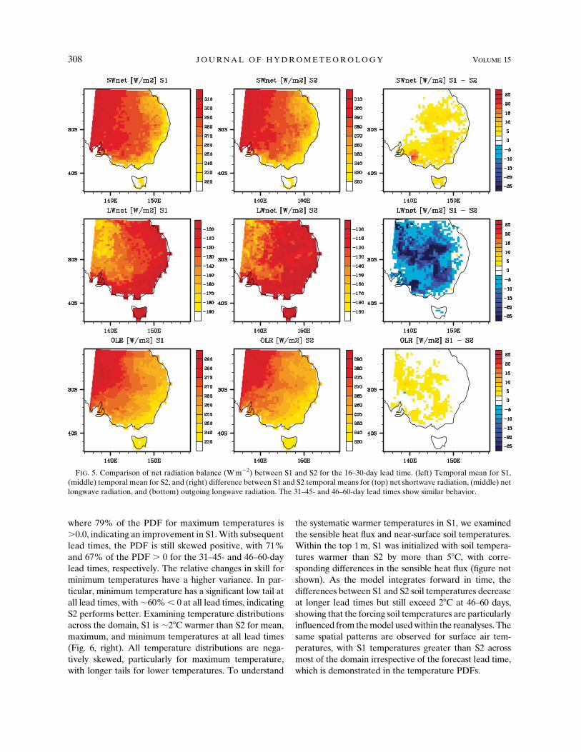
where 79% of the PDF for maximum temperatures is

.0.0, indicating an improvement in S1.With subsequent

lead times, the PDF is still skewed positive, with 71%

and 67% of the PDF . 0 for the 31–45- and 46–60-day

lead times, respectively. The relative changes in skill for

minimum temperatures have a higher variance. In par-

ticular, minimum temperature has a significant low tail at

all lead times, with;60%, 0 at all lead times, indicating

S2 performs better. Examining temperature distributions

across the domain, S1 is ;28C warmer than S2 for mean,

maximum, and minimum temperatures at all lead times

(Fig. 6, right). All temperature distributions are nega-

tively skewed, particularly for maximum temperature,

with longer tails for lower temperatures. To understand

the systematic warmer temperatures in S1, we examined

the sensible heat flux and near-surface soil temperatures.

Within the top 1m, S1 was initialized with soil tempera-

tures warmer than S2 by more than 58C, with corre-

sponding differences in the sensible heat flux (figure not

shown). As the model integrates forward in time, the

differences between S1 and S2 soil temperatures decrease

at longer lead times but still exceed 28C at 46–60 days,

showing that the forcing soil temperatures are particularly

influenced from themodel usedwithin the reanalyses. The

same spatial patterns are observed for surface air tem-

peratures, with S1 temperatures greater than S2 across

most of the domain irrespective of the forecast lead time,

which is demonstrated in the temperature PDFs.

FIG. 5. Comparison of net radiation balance (Wm22) between S1 and S2 for the 16–30-day lead time. (left) Temporal mean for S1,

(middle) temporal mean for S2, and (right) difference between S1 and S2 temporal means for (top) net shortwave radiation, (middle) net

longwave radiation, and (bottom) outgoing longwave radiation. The 31–45- and 46–60-day lead times show similar behavior.


FIG. 6. (left) PDFs, expressed as percentages, of the relative change in forecast skill between S1 and S2 formean

temperature (black), maximum temperatures (red), and minimum temperatures (blue) for three different lead

times: (top) 16–30, (middle) 31–45, and (bottom) 46–60 days. (right) Corresponding temperature (8C) PDFs for S1

(solid lines) and S2 (dashed lines).


The results for precipitation (Fig. 7) display limited

regions where the impact of the land surface initializa-

tion on forecast skill was significant. We examined the

resolution dependence of this result by aggregating our

results to a resolution comparable to Koster et al.

(2010), but we found there was no preferred land surface

initialization method for precipitation forecast skill.

b. Extreme soil moisture initialization and relativeforecast skill

The effect of the magnitude of the initial soil moisture

anomaly on the relative change in forecast skill was

assessed. We apply the same diagnostic to samples of

the 100 start dates corresponding to the S1 initial soil

moisture anomaly. Given that maximum temperatures

had the clearest results, we only present the results for

relative forecast skill associatedwith extreme soilmoisture

TABLE 1. Percentage of the area under the temperature PDF in

Fig. 6 (left) that corresponds to positive relative changes in forecast

skill.

Variable 16–30 days 31–45 days 46–60 days

Mean temperature 51 49 46

Maximum temperature 79 71 67

Minimum temperature 42 41 37

FIG. 7. As in Fig. 2, but for precipitation.


initialization formaximum temperature (Figs. 8, 9). There

is a tendency for the relative change in forecast skill to

increase in absolute magnitude, whether positive or

negative, with more extreme initial soil moisture anom-

alies (Fig. 8). The relative change in forecast skill for the

extreme terciles (Fig. 8, second column) show two regions

where the S1 skill exceeds S2 skill by approximately 20%

(5% more than those observed using all start dates). For

the extreme quintiles, there are isolated regions where

the S1 skill exceeds S2 by 30%, although for the 46–

60-day lead time, there is a large region where there is

a decrease in S1 skill relative to S2 of 15% that is greater

than the relative loss observed when using all dates. For

the extreme deciles, there are less data points available to

construct relative skill with less coherent change in skill

across the domain. However, only the relative gains ob-

served in Fig. 8 for the extreme terciles contain regions

where the relative gain in S1 skill is statistically signifi-

cant. Some of these statistically significant regions cor-

respond to those in Fig. 9 (left column) for all dates. For

the extreme quintiles and deciles (Fig. 9, right two col-

umns), there are no regions that are statistically signifi-

cant corresponding to those regions where there were

more extreme changes in relative forecast skill. However,

this is more likely due to the smaller sample size limiting

the ability to evaluate statistical significance.

We considered whether the relative change in forecast

skill had a dependency on wet or dry soil moisture

anomaly initialization as opposed to extreme soil mois-

ture initialization, where we differentiate between these

FIG. 8. (left to right) Relative gain in forecast skill for maximum 2-m air temperature, relative gain in forecast skill corresponding to the

start dates initialized with soil moisture content more extreme than the upper or lower terciles, relative gain in forecast skill for extreme

upper and lower quintiles, and relative gain in forecast skill for extreme upper and lower deciles for three different lead times: (top) 16–30,

(middle) 31–45, and (bottom) 46–60 days.


two classifications according to whether the initial soil

moisture anomaly was positive (wet) or negative (dry).

There was limited differentiation of the relative change

in forecast skill between the wet and dry cases for pre-

cipitation, mean temperature, and minimum tempera-

ture. For maximum temperature (Figs. 10, 11), the dry

case (Fig. 10, right) closely resembles the relative change

in forecast skill derived from that using all dates (Fig. 3,

left) with relative S1 gains of 10%–15% across most of

the domain for all lead times. The regions with larger

relative gains for S1 forecast skill are statistically sig-

nificant across all lead times (Fig. 11, right). For the wet

case (Fig. 10, left), there are some regions with S1 ex-

ceeding S2 skill by 30% up to 31–45 days into the fore-

cast period. At 46–60 days, S2 skill exceeds S1 by 20%

across almost half the domain; however, this is not sta-

tistically significant (Fig. 11, left). In fact, there are no

regions for the wet case where the relative change in

forecast skill is statistically significant. Again, this is

likely associated with the sample size, where there were

more extreme dry cases than wet cases, and may only be

particular to the 10-yr period that the simulations cover.

c. Comparison of forecast skill across all start dates

To capture whether the relative change in skill is the

same across all 10 start dates, rather than just those

corresponding to DJF, we plot the areal average of the

squared correlations (R2) corresponding to the 16–30-,

31–45-, and 46–60-day lead times for each start date and

series (Fig. 12). For precipitation (Fig. 12a) there is no

clear differentiation between S1 and S2. This is consis-

tent with Fig. 7, which showed no clear preference for

land surface initialization method across the lead times.

Note, in relation to Fig. 12a, R2 values of ;0.5 can be

FIG. 9. As in Fig. 8, but for corresponding p values.


considered high and a likely response to the lateral

boundary forcing. However, these values are not indic-

ative of the forecast skill attainable at longer lead times,

with some start dates indicating that the skill at the

46–60-day lead time is less than the skill at the 31–45-day

lead time. Similarly for the mean, maximum, and mini-

mum air temperatures, there is limited differentiation

between S1 and S2, although for maximum temperatures

FIG. 10. Relative gain in forecast skill between S1 and S2 for start dates initialized with a (left) wet and (right) dry

soil moisture anomaly for maximum 2-m air temperature for three different lead times: (top) 16–30, (middle) 31–45,

and (bottom) 46–60 days.


(Fig. 12c) S1 R2 exceeds S2 R2 for all start dates and lead

times, consistent with the relative gain in S1 forecast skill

shown in Fig. 3. For all variables in Fig. 12, the R2 for

both series are variable across the start dates, suggesting

some dependence upon the initial conditions at the be-

ginning of each forecast. There is a contrast in the R2

values between precipitation and temperature. For pre-

cipitation R2 values range between 0.30 and 0.50, with

FIG. 11. As in Fig. 10, but for corresponding p values.


higher values for the latter half of start dates. For mean

temperature, R2 values are between 0.60 and 0.90. The

R2 values for maximum temperature are within 0.70 and

0.90 and minimum temperature values are within 0.60

and 0.75, contributing to lower values in mean temper-

ature, particularly for start dates corresponding to late

summer and early autumn.

The potential predictability is defined as the squared

correlation between the model data with the ensemble

mean as the reference truth (Koster et al. 2010; van den

Hurk et al. 2012), and it provides a measure of the

maximum possible skill of the model system. Again, we

plot the areal average for both series for all lead times

and across each start date (Fig. 13). For all variables, S1

skill exceeds S2, particularly for mean and maximum

temperatures, illustrating that S1 has increased in-

ternally consistency compared to S2.

4. Discussion

Our results show that subseasonal forecast skill in

a regional climate model is sensitive to the land surface

initialization method. In particular, temperature fore-

casts show relative gains in forecast skill with initializa-

tion from prior offline simulations (S1), with the greatest

impact at shorter lead times of 16–30 days. The finer-

scale resolution of our simulations reveals greater spa-

tial variability in the impact of land surface initialization,

with some regions showing a decrease of skill. At longer

lead times, the magnitude of both positive and negative

FIG. 12. Time series of the squared correlations between WRF–LIS–CABLE with AWAP as the

reference truth, corresponding to each of the 10 start dates for (a) precipitation, (b) mean air tempera-

ture, (c) maximum air temperature, and (d) minimum air temperature for S1 (solid lines) and S2 (dashed

lines). Colors correspond to each start date: 1 Oct, dark blue; 15 Oct, blue; 1 Nov, light blue; 15 Nov, dark

green; 1 Dec, light green; 15Dec, yellow; 1 Jan, orange; 15 Jan, red; 1 Feb, violet; and 15 Feb, dark purple.


relative skill decrease, showing that as the model in-

tegrates forwards in time, the simulations converge.

The distinct regions of gains and losses in skill for

mean temperature were separated into maximum and

minimum temperatures. These show that using offline

simulations for land surface initialization is particularly

important for forecasting maximum temperatures with

coherent gains across the domain that were maintained

46–60 days into the forecast. The relative loss in S1 skill

for mean temperature across a large proportion of the

domain was associated with significant decreases in S1

skill for minimum temperature over corresponding re-

gions. These negative skill contributions indicate that

there are circumstances where using reanalyses to ini-

tialize the land surface can perform better for some

variables than using prior offline simulations.

Our result for minimum temperature was associated

with differences in the net longwave radiation between

the two series, particularly the outgoing longwave radi-

ation, which is largely determined by cloud cover. Dif-

ferences in net shortwave radiation were smaller and

did not correspond to the regions where the relative

forecast skill for minimum temperature was significantly

negative. A new result in this paper is the asymmetry

in the coupling of soil moisture with maximum tem-

peratures, as distinct from minimum temperatures. This

asymmetry has been observed before with the impact of

land cover change (Avila et al. 2012) and with the re-

sponse to increases in radiative forcing (Caesar et al.

2006; Alexander et al. 2006). In our experiments, the

asymmetry is relatively straightforward to explain. Soil

moisture affects the partitioning of net radiation be-

tween sensible and latent heat (Seneviratne et al. 2010).

During the day net radiation is dominated by solar ra-

diation. When latent heat is dominant, because soil

moisture is available, the boundary layer tends to be

FIG. 13. As in Fig. 12, but for the time series of the potential predictability, squared correlations between

WRF–LIS–CABLE with the ensemble mean as the reference truth.


cooler, shallower, and moister. When sensible heat is

dominant because soil moisture is limited, a dryer,

deeper, and warmer boundary layer is more common

(Betts 2009). Thus, during the day there are multiple

mechanisms that translate a change in soil moisture (or

an availability of soil moisture) into an impact on how

net radiation is partitioned and thereby into an impact

on maximum temperatures. In contrast, at night, net

radiation is dominated by the net exchange of longwave

radiation. Minimum temperatures tend to require clear

sky conditions at night that enable strong net emissions

of longwave radiation. Residual heating from the sur-

face through the soil heat flux is another component of

the surface energy balance that can impart a significant

influence on nighttime temperatures. Differences in the

soil temperature, arising from the different initialization

methods, may have contributed to the negative relative

S1 skill values for minimum temperatures. In general,

there is negligible coupling between the actual soil

moisture and cloud cover at night, and therefore. a strong

impact between soil moisture initialization and minimum

temperature is less likely. However, the potential for

coupling between soil temperature and minimum tem-

peratures through the soil heat flux may explain the

negative relative S1 skill values for minimum tempera-

tures associated with the differences in soil temperature

initialization. During the day, the soil heat flux is directed

downward, with the difference in soil temperature im-

parting less influence on surface temperature. An asym-

metry between the impact of soil moisture and soil

temperature initialization on maximum and minimum

temperatures is therefore the expected consequence of

the different processes that link these quantities with net

radiation.

For precipitation, the impact of land surface ini-

tialization is highly regionalized and there is no pre-

ferred land surface initialization method with respect

to relative forecast skill. Similar results were found by

Koster et al. (2010, 2011) and van den Hurk et al.

(2012). Despite running the forecasts at a finer spatial

scale to further resolve the geographical heterogene-

ity, limited gains in forecast skill for precipitation were

possible from prior offline simulations. Precipitation

over the domain is influenced by a range of synoptic-

scale weather systems, including cold fronts and east

coast lows (Risbey et al. 2009), which are defined to

some extent by the lateral boundary conditions. These

dominate the rainfall relative to the land surface bound-

ary conditions, as seen in Fig. 12, with the moderate skill

values of 40%–50%.

In general, both Koster et al. (2010) and van denHurk

et al. (2012) show that over time the impact of land

surface initialization degrades, with the largest change in

forecast skill within the first 30 days, and we observe

similar behavior in our results. One expects that as the

model integrates forward in time, whether one initializes

the model with or without equilibrated land surface

states, both cases will eventually converge. However,

this has some dependency on the initial soil moisture

state of the forecast, as shown in both Koster et al.

(2010) and van den Hurk et al. (2012), and potentially

for the model configuration employed. The extreme

terciles show a similar spatial distribution in the relative

forecast skill as that derived using all start dates. As one

reduces the sample size to sample dates corresponding

to more extreme soil moisture initialization, the impact

on relative forecast skill appears to be greater. However,

because of the small sample size, we are limited in

evaluating the statistical significance of this result.

Similarly, differences in the relative forecast skill be-

tween wet and dry soil initialization show that the initial

soil moisture state can contribute to the final forecast

skill. Our analysis of the forecast skill and potential

predictability across all start dates, October through to

April, shows that the impact of land surface initialization

on relative forecast skill has some dependence on the

antecedent soil moisture conditions at the initialization

of the forecast.

5. Conclusions

We have used WRF coupled to CABLE to evaluate

the sensitivity of simulation skill to two different ini-

tialization methods for a domain centered over south-

eastern Australia. Our results show that using land

surface states obtained from offline simulations con-

tribute relative gains in forecast skill for temperature of

10%–20% for the first 16–30 days of the forecast, with

limited gains in relative skill for precipitation. These

results are consistent with earlier studies that evaluate

the importance of land surface initialization (Koster

et al. 2010, 2011; van denHurk et al. 2012).We extended

the analysis to consider the asymmetry between maxi-

mum and minimum temperatures to understand the

spatial variability of the mean temperature response to

land surface initialization. We found that the strongest

gains in relative forecast skill for land surface initiali-

zation from prior offline simulations were apparent for

maximum temperature, with gains exceeding 20% in some

regions at up to 60 days into the forecast. In contrast, the

relative skill for minimum temperatures showed large

regions where land surface initialization from prior

offline simulation did not contribute to relative gains in

forecast skill, with land surface initialization from re-

analyses performing better. The contrasting response

to land surface initialization between maximum and


minimum temperatures was associated with different

soil moisture coupling mechanisms.

The results of Koster et al. (2010, 2011) and van den

Hurk et al. (2012) are based on a multimodel consensus

estimate. We have only run the experiment with a single

model configuration, so we cannot exclude the possi-

bility that our results are model dependent. However,

we show that the land surface initialization method ap-

plied in a regional climate model can have significant

implications for short-term simulations and the simula-

tion of processes that are sensitive to the land surface

state. In particular, the use of offline simulations to ini-

tialize soil moisture does improve the predictability for

temperature, particularly maximum temperature.

Acknowledgments. This study was supported by the

Australian Research Council Centre of Excellence for

Climate System Science Grant CE110001028. The com-

putational modeling was supported by the NCI National

Facility at the ANU, Australia. Annette Hirsch was

supported by an Australian Postgraduate Award and

CSIRO OCE Postgraduate Top Up Scholarship. The

authors thank Mark Decker for providing the bias-

corrected MERRA data, Scott Sisson for advice on

evaluating the statistical significance of our results, and

Randal Koster and Bart van den Hurk for clarification

on the GLACE-2 methodology. The authors would

also like to thank the anonymous reviewers who pro-

vided constructive comments on the manuscript.

REFERENCES

Abramowitz, G., A. J. Pitman, H. Gupta, E. Kowalczyk, and

Y. Wang, 2007: Systematic bias in land surface models.

J. Hydrometeor., 8, 989–1001, doi:10.1175/JHM628.1.

——, R. Leuning, M. Clark, and A. J. Pitman, 2008: Evaluating the

performance of land surfacemodels. J. Climate, 21, 5468–5481,

doi:10.1175/2008JCLI2378.1.

Alexander, L. V., and Coauthors, 2006: Global observed changes

in daily climate extremes of temperature and precipitation.

J. Geophys. Res., 111, D05109, doi:10.1029/2005JD006290.

Avila, F. B., A. J. Pitman, M. G. Donat, L. V. Alexander, and

G. Abramowitz, 2012: Climate model simulated changes in

temperature extremes due to land cover change. J. Geophys.

Res., 117, D04108, doi:10.1029/2011JD016382.

Beljaars, A. C. M., P. Viterbo, and M. J. Miller, 1996: The

anomalous rainfall over the United States during July 1993:

Sensitivity to land surface parameterization and soil mois-

ture anomalies. Mon. Wea. Rev., 124, 362–383, doi:10.1175/

1520-0493(1996)124,0362:TAROTU.2.0.CO;2.

Betts, A. K., 2009: Land-surface-atmosphere coupling in observa-

tions and models. J. Adv. Model. Earth Syst., 1, doi:10.3894/

JAMES.2009.1.4.

Caesar, J., L. Alexander, and R. Vose, 2006: Large-scale changes in

observed daily maximum and minimum temperatures: Crea-

tion and analysis of a new gridded data set. J. Geophys. Res.,

111, D05101, doi:10.1029/2005JD006280.

Clapp, R. B., and G. M. Hornberger, 1978: Empirical equations for

some soil hydraulic properties. Water Resour. Res., 14, 601–

604, doi:10.1029/WR014i004p00601.

Cruz, F. T., A. J. Pitman, and Y. Wang, 2010: Can the stomatal re-

sponse to higher atmospheric carbon dioxide explain the unusual

temperatures during the 2002 Murray–Darling Basin drought.

J. Geophys. Res., 115, D02101, doi:10.1029/2009JD012767.

Decker, M., A. J. Pitman, and J. P. Evans, 2013: Groundwater

constraints on simulated transpiration variability over south-

eastern Australian forests. J. Hydrometeor., 14, 543–559,

doi:10.1175/JHM-D-12-058.1.

Dee, D. P., and Coauthors, 2011: The ERA-Interim reanalysis:

Configuration and performance of the data assimilation sys-

tem. Quart. J. Roy. Meteor. Soc., 137, 553–597, doi:10.1002/

qj.828.

deNoblet-Ducoudr�e, N., and Coauthors, 2012: Determining robust

impacts of land-use-induced land cover changes on surface

climate over North America and Eurasia: Results from the

first set of LUCID experiments. J. Climate, 25, 3261–3281,

doi:10.1175/JCLI-D-11-00338.1.

Douville, H., 2010: Relative contribution of soil moisture and snow

mass to seasonal climate predictability: A pilot study. Climate

Dyn., 34, 797–818, doi:10.1007/s00382-008-0508-1.

——, and F. Chauvin, 2000: Relevance of soil moisture for seasonal

climate predictions: A preliminary study. Climate Dyn., 16,

719–736, doi:10.1007/s003820000080.

Dudhia, J., 1989: Numerical study of convection observed dur-

ing the winter monsoon experiment using a mesoscale two-

dimensional model. J. Atmos. Sci., 46, 3077–3107, doi:10.1175/

1520-0469(1989)046,3077:NSOCOD.2.0.CO;2.

Evans, J. P., and M. F. McCabe, 2010: Regional climate simula-

tion over Australia’s Murray-Darling basin: Amultitemporal

assessment. J. Geophys. Res., 115, D14114, doi:10.1029/

2010JD013816.

——, and S. Westra, 2012: Investigating the mechanisms of diurnal

rainfall variability using a regional climate model. J. Climate,

25, 7232–7247, doi:10.1175/JCLI-D-11-00616.1.

——, A. J. Pitman, and F. T. Cruz, 2011: Coupled atmospheric and

land surface dynamics over southeast Australia: A review,

analysis and identification of future research priorities. Int. J.

Climatol., 31, 1758–1772, doi:10.1002/joc.2206.

——, M. Ekstr€om, and F. Ji, 2012: Evaluating the performance of

a WRF physics ensemble over south-east Australia. Climate

Dyn., 39, 1241–1258, doi:10.1007/s00382-011-1244-5.Fennessy, M. J., and J. Shukla, 1999: Impact of initial soil wetness

on seasonal atmospheric prediction. J. Climate, 12, 3167–3180,

doi:10.1175/1520-0442(1999)012,3167:IOISWO.2.0.CO;2.

Haverd, V., and Coauthors, 2012: Multiple observation types re-

duce uncertainty in Australia’s terrestrial carbon and water

cycles. Biogeosci. Discuss., 9, 12 181–12 258.

Hong, S. Y., Y. Noh, and J. Dudhia, 2006: A new vertical diffusion

package with an explicit treatment of entrainment processes.

Mon. Wea. Rev., 134, 2318–2341, doi:10.1175/MWR3199.1.

Jaeger, E. B., and S. I. Seneviratne, 2011: Impact of soil moisture–

atmosphere coupling on European climate extremes and

trends in a regional climate model. Climate Dyn., 36, 1919–

1939, doi:10.1007/s00382-010-0780-8.

Jones, D., W. Wang, and R. Fawcett, 2009: High-quality spatial

climate data-sets for Australia. Aust. Meteor. Mag., 58,

233–248.

Kain, J. S., 2004: The Kain–Fritsch convective parameteriza-

tion: An update. J. Appl. Meteor., 43, 170–181, doi:10.1175/

1520-0450(2004)043,0170:TKCPAU.2.0.CO;2.


——, and J. M. Fritsch, 1990: A one-dimensional entraining de-

training plume model and its application in convective pa-

rameterization. J. Atmos. Sci., 47, 2784–2802, doi:10.1175/

1520-0469(1990)047,2784:AODEPM.2.0.CO;2.

——, and ——, 1993: Convective parameterization for mesoscale

models: The Kain–Fritsch scheme. The Representation of

Cumulus Convection in Numerical Models, Meteor. Monogr.,

No. 46, Amer. Meteor. Soc., 165–170.

King, A. D., L. V. Alexander, and M. G. Donat, 2013: The efficacy

of using gridded data to examine extreme rainfall character-

istics: A case study for Australia. Int. J. Climatol., 33, 2376–

2387, doi: 10.1002/joc.3588.

Koster, R. D., and Coauthors, 2006: GLACE: The Global Land–

Atmosphere Coupling Experiment. Part I: Overview. J. Hy-

drometeor., 7, 590–610, doi:10.1175/JHM510.1.

——, Z. Guo, R. Yang, P. A. Dirmeyer, K. Mitchell, and M. J.

Puma, 2009: On the nature of soil moisture in land surface

models. J. Climate, 22, 4322–4335, doi:10.1175/2009JCLI2832.1.

——, and Coauthors, 2010: Contribution of land surface initiali-

zation to subseasonal forecast skill: First results from a

multi-model experiment. Geophys. Res. Lett., 37, L02402,

doi:10.1029/2009GL041677.

——, and Coauthors, 2011: The second phase of the Global Land–

Atmosphere Coupling Experiment: Soil moisture contri-

butions to subseasonal forecast skill. J. Hydrometeor., 12,

805–822, doi:10.1175/2011JHM1365.1.

Kowalczyk, E. A., and Coauthors, 2013: The land surface model

component of ACCESS: Description and impact on the simu-

lated surface climatology. Aust. Meteor. Oceanogr. J., 63, 65–82.

Kumar, S. V., and Coauthors, 2006: Land information system: An

inter-operable framework for high resolution land surface

modeling.Environ. Model. Software, 21, 1402–1415, doi:10.1016/

j.envsoft.2005.07.004.

Mlawer, E. J., S. J. Taubman, P. D. Brown, M. J. Lacono, and S. A.

Clough, 1997: Radiative transfer for inhomogeneous atmo-

sphere: RRTM, a validated correlated-k model for the long-

wave. J. Geophys. Res., 102 (D14), 16 663–16 682, doi:10.1029/

97JD00237.

Peters-Lidard, C. D., and Coauthors, 2007: High-performance

earth system modeling with NASA/GSFC’s land information

system. Innovations Syst. Software Eng., 3, 157–165, doi:10.1007/s11334-007-0028-x.

Pitman, A. J., F. B. Avila, G. Abramowitz, Y. P.Wang, S. J. Phipps,

and N. de Noblet-Ducoudr�e, 2011: Importance of background

climate in determining impact of land–cover change on re-

gional climate. Nat. Climate Change, 1, 472–475, doi:10.1038/

nclimate1294.

Raupach, M. R., K. Finkele, and L. Zhang, 1997: SCAM (Soil-

Canopy-Atmosphere Model): Description and comparison

with field data. Tech. Rep. 132, CSIRO Centre for Environ-

mental Mechanics, Canberra, ACT, Australia, 81 pp.

Reichle, R. H., R. D. Koster, G. J. M. de Lannoy, B. A. Forman,

Q. Liu, S. P. P. Mahanama, and A. Tour�e, 2011: Assessment

and enhancement ofMERRA land surface hydrology estimates.

J. Climate, 24, 6322–6338, doi:10.1175/JCLI-D-10-05033.1.

Risbey, J. S., M. J. Pook, P. C. McIntosh, M. C.Wheeler, and H. H.

Hendon, 2009:On the remote drivers of rainfall variability in

Australia. Mon. Wea. Rev., 137, 3233–3253, doi:10.1175/

2009MWR2861.1.

Santanello, J. A., C. D. Peters-Lidard, and S. V. Kumar, 2011:

Diagnosing the sensitivity of local land–atmosphere coupling

via the soil moisture–boundary layer interaction. J. Hydro-

meteor., 12, 766–786, doi:10.1175/JHM-D-10-05014.1.

——, ——, A. Kennedy, and S. V. Kumar, 2013: Diagnosing the

nature of land–atmosphere coupling: A case study of dry/wet

extremes in the U.S. southern Great Plains. J. Hydrometeor.,

14, 3–24, doi:10.1175/JHM-D-12-023.1.

Seneviratne, S. I., T. Corti, E. L. Davin, M. Hirschi, E. B. Jaeger,

I. Lehner, B. Orlowsky, and A. J. Teuling, 2010: Investigating

soil moisture–climate interactions in a changing climate:

A review. Earth Sci. Rev., 99, 125–161, doi:10.1016/

j.earscirev.2010.02.004.

Skamarock, W. C., and Coauthors, 2008: A description of the

AdvancedResearchWRF version 3. NCARTech. NoteNCAR/

TN-4751STR, 113 pp. [Available online at http://www.mmm.

ucar.edu/wrf/users/docs/arw_v3.pdf.]

Timbal, B., S. Power, R. Colman, J. Viviand, and S. Lirola, 2002:

Does soil moisture influence climate variability and predict-

ability over Australia? J. Climate, 15, 1230–1238, doi:10.1175/

1520-0442(2002)015,1230:DSMICV.2.0.CO;2.

van den Hurk, B., F. Doblas-Reyes, G. Balsamo, R. D. Koster,

S. I. Seneviratne, and H. Camargo Jr., 2012: Soil moisture

effects on seasonal temperature and precipitation forecast

scores in Europe. Climate Dyn., 38, 349–362, doi:10.1007/s00382-010-0956-2.

Wang, Y. P., E. Kowalczyk, R. Leuning, G. Abramowitz, M. R.

Raupach, B. Pak, E. van Gorsel, and A. Luhar, 2011: Di-

agnosing errors in a land surface model (CABLE) in the time

and frequency domains. J. Geophys. Res., 116, G01034,

doi:10.1029/2010JG001385.

Zhang, Q., Y. P. Wang, A. J. Pitman, and Y. J. Dai, 2011: Limita-

tions of nitrogen and phosphorous on the terrestrial carbon

uptake in the 20th century. Geophys. Res. Lett., 38, L22701,

doi:10.1029/2011GL049244.


Impact of Land Surface Initialization Approach on Subseasonal Forecast...

Documents

Transcript of Impact of Land Surface Initialization Approach on Subseasonal Forecast...