IMPACT OF FOREIGN DIRECT INVESTMENT(FDI) ON DOMESTIC ...

© UIJIR | ISSN (O) – 2582-6417

AUGUST 2021 | Vol. 2 Issue 3 www.uijir.com

Universe International Journal of Interdisciplinary Research

(Peer Reviewed Refereed Journal)

DOI: https://www.doi-ds.org/doilink/09.2021-17798463/UIJIR www.uijir.com

25

IMPACT OF FOREIGN DIRECT INVESTMENT(FDI) ON DOMESTIC

AGRICULTURAL PRODUCTION (DAP) IN NIGERIA: EVIDENCE FROM

ARDL MODEL APPLICATION (1981-2018)

Author’s Name: Mr. Ali, Ayuba1, Mr. Adejo, Moses Adejo2, Mrs. Obekpa, Hephzibah Onyeje3, Mr. Frimpong,

Ebenezer4,

Affiliation: 1Federal University of Agriculture Makurdi, PMB2373, Benue State, Nigeria, 2Department of

Agribusiness, Corvinus University of Budapest, Hungary.

E-Mail: [email protected]

DOI No. – 08.2020-25662434

Abstract

Increase in Domestic Agricultural Productivity (DAP) is germane for food security and employment of our

increasing population in Nigeria. This study determined the impact of Foreign Direct Investment (FDI) on the

domestic agricultural production with evidence from Autoregressive Distributed Lag (ARDL) model using time

series data that spans from 1981-2018. The findings from the growth model affirms a positive growth in FDI and

domestic agricultural production as found in previous studies. The result suggests that FDI has positive impact on

domestic agricultural production in the long run and short run. The result also shows that the present value of

domestic agricultural production will predict future values of FDI. Therefore, policies to attract inflows of FDI to

agriculture are suggested while limitations of the study as well as direction for future research are discussed.

Keywords: FDI, Domestic Agricultural Productivity (DAP), ARDL Model, Causal Relationship, Nigeria

INTRODUCTION

Domestic Agriculture plays an important role in the growth of any country, and this is more so

in Africa, where it directly and indirectly supports the survival and well-being of 70% of its

population and contributes over 20% to the Gross Domestic Product (GDP) (Nchuchume and

Adejuwon, 2012; Wiggins, Farrington, Henley, Grist, & Anne, 2013;). Agriculture accounts for

40% of the Gross Domestic Product (GDP) in Nigeria and employs about 70% of the working

population. (CIA, 2020). Nigeria currently faces many challenges. The core of the challenges

relates to unemployment and food insecurity. Food production in Nigeria is inadequate and

needs a significant amount of agricultural spending because of the constraints of agricultural

technologies and adverse weather conditions (Awunyo and Sackey, 2018).

Foreign Direct Investment (FDI) is the inflow by investment (setting aside money or resources

to obtain beneficial returns, such as interest, dividends or value appreciation) of foreign income

into a particular economy involving multinational corporations (Agba et al., 2018). Foreign

direct investment, according to the Organization for Economic Cooperation and Development

(OECD,2008), represents the purpose of creating a permanent interest of a resident enterprise

in a single economy (direct investor) in an enterprise (direct investment enterprise) residing in

an economy other than that of a direct investor. The presence of a long-term relationship

between the direct investor and the direct investment enterprise and a substantial degree of

control on the management of the enterprise indicates a lasting interest.

Evidence from Falki (2009) noted that Growing jobs, increasing production, improving exports

and increasing the speed of technology transfer are normally believed to be the effects of FDI on

mailto:[email protected]

© UIJIR | ISSN (O) – 2582-6417





Page 126

the host economy. FDI's potential benefits are that it promotes the use and utilization of local

raw materials, incorporates modern management and marketing methods and facilitates access

to emerging technologies. Aremu (1997) also noted that as one of the world's developing

countries, Nigeria has taken a range of steps aimed at accelerating domestic economic growth

and development, one of which is to attract foreign direct investment (FDI) into the country.

In the light of the significance of FDI on domestic agricultural productivity, a considerable

amount of literature has grown up to investigate different factors that could be responsible for

the slow performance of the domestic agricultural sector in Nigeria. Some of the factors includes

micro and macro-economic factors like Labour cost, cost of inputs, exchange rate, GDP, inflation

rate and agricultural policies like food importation (Adedeji and Okocha, 2011; Akpan, 2012;

Akpan et al., 2012; Kareem et al., 2013; Oloyede, 2014; Oluwatoyese et al., 2016; Edet and

Akpan, 2019). Earlier studies have not considered factors such as non-linearity and structural

breaks, and it is an established fact that most time series data do not exhibit a linear trend (Meo

et al. 2018; Meo et al., 2020).

The research aims to examine the influence of foreign direct investment on the domestic

agricultural productivity growth in Nigeria and make judicious use of its potentials and returns

to improve the standard of living in Nigeria. While it is possible for FDI to have high returns to

the output of the domestic agricultural productivity, and also want to examine the

counterfactual.

First, we have chosen the domestic agricultural productivity because domestic agriculture

contributes a fair share of Nigeria’s GDP relative to other sectors in the country, therefore

agriculture remains germane to Nigeria’s economic development.

Secondly, because of the volatility of oil price and the fall in revenue from the oil sector over the

years, the focus of the government is now shifting to domestic agriculture as a source of revenue

to fund our budget and also reduce the high rate of unemployment.

Unlike previous studies that focused on exchange rate and other macro-economic variables on

the agricultural sector, the research aims to add knowledge to growing area of research by

exploring the impact of foreign direct investment on domestic agricultural productivity in

Nigeria using the ARDL model that is tried and tested considering fractional disintegration,

small sample size as ours, non-linear relationship and endogeneity problem. The methodology

employed is a reason the study was embarked on as a linear model might produce inaccurate

results. We use the non-linear ARDL to solve these problems highlighted. The study also uses

the most recent data available that spans from 1981 to 2019, a time period that captures the

triple whammy of high inflation, recession, and the farmer-herder’s conflict in the country,

while also controlling for other significant variables.

This research work has been structured considering the review knowledge to literature which

explains relevant empirical studies, methodology which explains the data and method

employed, results and discussion displays and explains the result from the analysis while the

concluding remarks, policy direction and suggestion for further studies are presented in the

conclusion.

LITERATURE REVIEW

A plethora of studies exists with arguments from different school of thought on the magnitude

© UIJIR | ISSN (O) – 2582-6417





Page 127

of foreign direct investment on the development of domestic agricultural sector in developing

economies including Nigeria. It has been envisaged by the neoclassical and endogenous theory

that both private and public capital inflows enhance economic growth and development.

According to Edewor et al. (2018), the existence of Foreign Direct Investment and its attendant

growth can be broadly explained by the neo-classical theory of economic growth and the

investment theory, also known as the ‘two-gap model’. Dunning and Sarianna (2008), made a

submits that Foreign Direct Investment has the capacity to bring about positive growth as a

direct relationship exists between growth and increased productivity. Fisher and Gelb (1991),

due to the investment of Transnational Corporations (TNCs) in developing regions serving as

host affiliations related to these Transnational Corporations, there is resultant transfer of

technology and fund to these affiliations thereby transforming them into global networks of

research and development.

Furthermore, the growth of enterprises is enhanced as Foreign Direct Investment leads to trade

openness, thereby providing access to foreign markets, which in turn creates employment

opportunities, stimulating domestic demand of inputs from suppliers. The enhancement of trade

openness by FDI, enables an environment where new enterprises outside the borders of the

domestic economies hosting the affiliations of Transnational Corporations (Apter, 1965). A

contrasting argument exists by advocates of the Dependency theory opposing the positivity of

Foreign Direct Investment. Their submission sees FDI as a disguised tool used by developed

economies to control the economies of the developing regions (Bailey, 1995; Ake, 1996).

Also part of their argument is that the penetration of host economies by foreign investors would

bring about ‘disarticulated development’, which can also cause underdevelopment.

• Foreign Direct Investment and Domestic Agricultural Productivity

According to Msuya (2007), the adoption of new and advanced technologies cannot be

overemphasized as it enhances growth in domestic agricultural productivity. But a limitation

exists as local farmers find it difficult to adopt such advanced technologies due inadequate

income and lack of access to credit facilities, believed to be tackled by the financial and

technological support of Foreign Direct Investment.

The importance of FDI in agricultural growth is further buttressed by a study carried out by

Binuyo (2014) assessed the impact of FDI on the development of the agricultural sector in the

Nigerian economy, for a period of 1981 to 2012.

Also, Agba et al. (2018) conducted a research which was directed in answering the question

whether Foreign Direct Investments impacts Agricultural output in Nigeria. The study made

use of time series data which spanned a period of 34 years (1981-2014), with variables such

as the Agricultural Gross Domestic Product, Foreign Direct Investment, Exchange rate,

Interest rate, employment and Gross Capital Formation. From the Error Correction Model

(ECM) method used to analyze the impact of the variables showed that Foreign Direct

Investment positively affected Agricultural output, but this effect was only significant in the

long-run, while it was positive and insignificant in the short-run. This positive long-run effect

was seen in other variable like interest rate, exchange rate and employment.

Furthermore, a study which sought to determine the relationship between Foreign Direct

Investment to the agricultural sector and economic growth in Ghana, was conducted by

Awunyo-Victor and Sackey (2018). Error Correction Model (ECM) was also applied to

analyze the effect of the selected variables (Gross Domestic Product, Foreign Direct

© UIJIR | ISSN (O) – 2582-6417





Page 128

Investment in agriculture), with time series data collected from 1975 to 2018. The result

showed a significant positive relationship exists between the Foreign Direct Investment in

agriculture and economic growth in Ghana. Evidence of the effect of Foreign Direct

Investment in the growth of Agricultural Sector is seen in the Study conducted by Akinwale

et al. (2018) which employed the Error Correction Model technique to examine the effect of

Foreign Direct Investment, Nigeria’s government agricultural expenditure on agricultural

productivity and bank credit. The data on variables used were collected from 1986 to 2015.

The result revealed that FDI had significant direct relationship on Agricultural productivity,

implying that a unit change in FDI will cause a significant change in Agricultural

productivity in same direction. Government expenditure and Bank credit to Agricultural

Sector had a direct relationship with agricultural productivity best was insignificant.

Umechukwu and Okezie, C. A. (2018) conducted a study which sought to examine the

impact of Foreign Direct Investment on the agricultural sector in Nigeria, while making use

of Ordinary Least Square to estimate the time series data obtained for the period of 1990 to

2014. The study made use of variable such as Agricultural Sector GDP, Foreign Direct

Investment inflow to agriculture, Exchange rate, Inflation rate, Trade openness and Natural

resource flow. The effect of FDI on the agricultural sector was examined over the different

policy periods combined.

It further revealed that the impact of Foreign Direct Investment on the agricultural sector was

more during the pre-deregulated period compared to the deregulated period.

According to a Study by Ugwuegbe et al. (2013), growth model through the Ordinary Least

Square method was adopted to investigate the relationship between FDI and economic

growth in Nigeria.

Time series data for variables like Gross Domestic Product, Gross Fixed Capital Formation,

Foreign Direct Investment, Exchange rate and Interest rate, were collected over a period of

1981 to 2009. The result revealed a positive insignificant impact of both Foreign Direct

Investment and Interest rate on the economics, over the period under consideration which the

impact of Gross Fixed Capital Formation and Exchange rate were found to be positive and

significant.

A study by Iddrisu, et al. (2015) which looked at the impact of Foreign Direct Investment on

the Ghanaian agricultural sector, using the Vector Error Correction Model (VECM) analytical

technique, found that FDI positively impact the productivity of the agricultural sector in the

short run, but has a negative impact on the agricultural sector productivity in the long run,

during the considered period of 1980 to 2013. Variables included in the model include FDI,

Trade openness, Value Addition Constant in Agriculture, Inflation rate, Exchange rate, and

Gross Fixed Capital Formation. The study also observed a deformation in the country’s

currency (Cedi) which negatively impacted the long run growth at the agricultural sector

because of high cost associated with imported inputs and machinery necessary to enhance

agricultural productivity in the country.

Amongst these previous studies by researchers, one common observation remains how

foreign direct investment has influenced the growth of the Agricultural sector, especially in

developing economies. Also, most of the research in this line made use of the Vector Error

Correction Model (VECM) as the technique to determine the impact of FDI on growth of

either the agricultural subsector or the economy as a whole. The relevance of this Study is

seen as it employs the Autoregressive Distributed Lagged Model with the Bounds testing

© UIJIR | ISSN (O) – 2582-6417





Page 129

approach to examine the influence of foreign direct investment on Nigeria’s domestic

production in the agricultural sector while covering a more period of 1981 to 2018.

METHEDOLOGY

1. Variables

To examine the economic impact on how foreign direct investment relates with domestic

agricultural productivity in Nigeria, the study uses time series data. Table 1 shows all the

variables used in this research and their sources. In order to obtain more meaningful

insight, logarithmic transformation of these variables was adopted to remove large and

extreme bias that might be associated with the variables.

Table 1: Definition of variables Variables Measurement Source Symbol

Domestic agricultural productivity Naira equivalent CBN annual report DProd FDI to agriculture Naira to USD equivalent CBN annual report FDI

Exchange rate Naira to USD equivalent CBN annual report Exch Rate Labour

Inflation rate Interest rate

Number of persons involved in agric. In % equivalent In % equivalent

CBN annual report CBN annual report CBN annual report

AGRL INFL INTR

Source: Author’s Compilation (2020)

2. Data Analysis Techniques

The unit root test was carried out on all variables. In addition to the Dickey and Fuller

(1981) process, the Phillip and Perron (1989) test was used to check for the unit root

presence in each variable (an indication for non-stationarity). This is because the use of unit

roots identified in data can lead to significant statistical inference errors, the lag length

structure was used to select the model lag length. The Zivot and Andrews (1992) test, a third

test, was used to check for bias when a structural break is present, a weakness not addressed

in the previous two tests. To test for structural break in the sequence, the Chow test was

used. The growth model was used to determine the domestic productivity growth path,

ARDL was used to figure out long-term and short-term effect of FDI on domestic

agricultural productivity, and granger causality indicating how to figure out the existence of

causal relationship between domestic agricultural productivity in Nigeria and FDI. The

Growth Model was used to evaluate the pattern and growth rates of Foreign Direct

Investment and Domestic Agricultural Productivity. The Granger Causality Test was used to

analyze the causal relationship between Foreign Direct Investment and Domestic

Agricultural Productivity, while the Bounds Testing technique was used to figure out the

influence of FDI on Domestic Agricultural Productivity. From the Granger Causality test

results and the Autoregressive Distributed Lag model, the hypotheses were checked. The

logarithmic transformation of these variables was introduced in order to gain more

meaningful insight. Using the Augmented Dickey Fuller (ADF) method, the unit root tests of

all variables were carried out. The Jarque-Bera test was also used to check the correctness of

the fit of the data to see whether a normal distribution was followed. The Growth model for

the variables of interest is specified below:

© UIJIR | ISSN (O) – 2582-6417





Page 130

lnYt = α + βAGDPt + µt . . . . . . . (i)

lnYt = α + βFDIt + µt . . . . . . . (ii)

Where,

α = intercept.

β = vector of the trend variable and µ is the econometric error term.

βAGDP, βFDI = coefficients of the trend variables for Agricultural Gross Domestic Product

(AGDP) and Foreign Direct Investment (FDI).

Following Oyinbo and Rekwot (2014), the constant term and trend Augmented Dickey

Fuller (ADF) model is defined as follows:

titi

p

i

tt YYtY ++++= −

=

− 1

110

. . . . (iii)

Where,

Y = variables of interest (domestic agricultural productivity, foreign direct investment,

exchange rate, inflation rate and interest rate, ).

0 = constant.

1 = coefficient of the trend series. p = lag order of the autoregressive process.

1−tY= is lagged value of order one of 1−tY

t = error term.

The system for the Autoregressive Distributed Lag (ARDL) model is specified as follows:

𝑙𝑛𝐷𝑃𝑟𝑜𝑑𝑡−𝑖 = 𝑎0 + 𝑎1𝑙𝑛𝐹𝐷𝐼𝑡−𝑖 + 𝑎2𝑙𝑛𝐸𝑋𝐺𝑅𝑡−𝑖 + 𝑎3𝑙𝑛𝐼𝑁𝐹𝑅𝑡−𝑖 + 𝑎4𝑙𝑛𝐼𝑁𝑇𝑅𝑡−𝑖 +

𝑎5𝑙𝑛𝐴𝐺𝑅𝐿𝑡−𝑖 + 𝑎6𝑙𝑛𝐺𝐹𝐶𝐹𝑡−𝑖 + 𝑎7𝑙𝑛𝐴𝑃𝑡−𝑖 + 𝜕𝐸𝐶𝑀1𝑡 + 𝑢1𝑡 … … … (𝑖𝑣)

𝑙𝑛𝐹𝐷𝐼𝑡−𝑖 = 𝑎0 + 𝑎1𝑙𝑛𝐷𝑃𝑟𝑜𝑑𝑡−𝑖 + 𝑎2𝑙𝑛𝐸𝑋𝐺𝑅𝑡−𝑖 + 𝑎3𝑙𝑛𝐼𝑁𝐹𝑅𝑡−𝑖 + 𝑎4𝑙𝑛𝐼𝑁𝑇𝑅𝑡−𝑖 +

𝑎5𝑙𝑛𝐴𝐺𝑅𝐿𝑡−𝑖 + 𝑎6𝑙𝑛𝐺𝐹𝐶𝐹𝑡−𝑖 + 𝑎7𝑙𝑛𝐹𝐷𝐼𝑡−𝑖 + 𝜕𝐸𝐶𝑀2𝑡 + 𝑢2𝑡 … … … (𝑣)

𝑙𝑛𝐸𝑋𝐺𝑅𝑡−𝑖 = 𝑎0 + 𝑎1𝑙𝑛𝐷𝑃𝑟𝑜𝑑𝑡−𝑖 + 𝑎2𝑙𝑛𝐹𝐷𝐼𝑡−𝑖 + 𝑎3𝑙𝑛𝐼𝑁𝐹𝑅𝑡−𝑖 + 𝑎4𝑙𝑛𝐼𝑁𝑇𝑅𝑡−𝑖 +

𝑎5𝑙𝑛𝐴𝐺𝑅𝐿𝑡−𝑖 + 𝑎6𝑙𝑛𝐺𝐹𝐶𝐹𝑡−𝑖 + 𝑎7𝑙𝑛𝐸𝑋𝐺𝑅𝑡−𝑖 + 𝜕𝐸𝐶𝑀3𝑡 + 𝑢3𝑡 … … … (𝑣𝑖)

𝑙𝑛𝐼𝑁𝐹𝑅𝑡−𝑖 = 𝑎0 + 𝑎1𝑙𝑛𝐷𝑃𝑟𝑜𝑑𝑡−𝑖 + 𝑎2𝑙𝑛𝐹𝐷𝐼𝑡−𝑖 + 𝑎3𝑙𝑛𝐸𝑋𝐺𝑅𝑡−𝑖 + 𝑎4𝑙𝑛𝐼𝑁𝑇𝑅𝑡−𝑖 +

𝑎5𝑙𝑛𝐴𝐺𝑅𝐿𝑡−𝑖 + 𝑎6𝑙𝑛𝐺𝐹𝐶𝐹𝑡−𝑖 + 𝑎7𝑙𝑛𝐼𝑁𝐹𝑅𝑡−𝑖 + 𝜕𝐸𝐶𝑀4𝑡 + 𝑢4𝑡 … … … (𝑣𝑖𝑖)

𝑙𝑛𝐼𝑁𝑇𝑅𝑡−𝑖 = 𝑎0 + 𝑎1𝑙𝑛𝐷𝑃𝑟𝑜𝑑𝑡−𝑖 + 𝑎2𝑙𝑛𝐹𝐷𝐼𝑡−𝑖 + 𝑎3𝑙𝑛𝐸𝑋𝐺𝑅𝑡−𝑖 + 𝑎4𝑙𝑛𝐼𝑁𝐹𝑅𝑡−𝑖 +

𝑎5𝑙𝑛𝐴𝐺𝑅𝐿𝑡−𝑖 + 𝑎6𝑙𝑛𝐺𝐹𝐶𝐹𝑡−𝑖 + 𝑎7𝑙𝑛𝐼𝑁𝑇𝑅𝑡−𝑖 + 𝜕𝐸𝐶𝑀5𝑡 + 𝑢5𝑡 … … (𝑣𝑖𝑖𝑖)

𝑙𝑛𝐴𝐺𝑅𝐿𝑡−𝑖 = 𝑎0 + 𝑎1𝑙𝑛𝐷𝑃𝑟𝑜𝑑𝑡−𝑖 + 𝑎2𝑙𝑛𝐹𝐷𝐼𝑡−𝑖 + 𝑎3𝑙𝑛𝐸𝑋𝐺𝑅𝑡−𝑖 + 𝑎4𝑙𝑛𝐼𝑁𝐹𝑅𝑡−𝑖 +

𝑎5𝑙𝑛𝐼𝑁𝑇𝑅𝑡−𝑖 + 𝑎6𝑙𝑛𝐺𝐹𝐶𝐹𝑡−𝑖 + 𝑎7𝑙𝑛𝐴𝐺𝑅𝐿𝑡−𝑖 + 𝜕𝐸𝐶𝑀7𝑡 + 𝑢7𝑡 … … … (𝑖𝑥)

© UIJIR | ISSN (O) – 2582-6417





Page 131

Where,

𝐷𝑃𝑟𝑜𝑑𝑡−𝑖 = 𝐷𝑜𝑚𝑒𝑠𝑡𝑖𝑐 𝐴𝑔𝑟𝑖𝑐𝑢𝑙𝑡𝑢𝑟𝑎𝑙 𝑃𝑟𝑜𝑑𝑢𝑐𝑡𝑖𝑣𝑖𝑡𝑦 (𝑛𝑎𝑖𝑟𝑎)

𝐹𝐷𝐼𝑡−𝑖 = 𝐹𝑜𝑟𝑒𝑖𝑔𝑛 𝐷𝑖𝑟𝑒𝑐𝑡 𝐼𝑛𝑣𝑒𝑠𝑡𝑚𝑒𝑛𝑡 (𝑈𝑆 𝑑𝑜𝑙𝑙𝑎𝑟𝑠)

𝐸𝑋𝐺𝑅𝑡−𝑖 = 𝐸𝑥𝑐ℎ𝑎𝑛𝑔𝑒 𝑅𝑎𝑡𝑒 (𝑑𝑜𝑙𝑙𝑎𝑟/𝑛𝑎𝑖𝑟𝑎)

𝐼𝑁𝐹𝑅𝑡−𝑖 = 𝐼𝑛𝑓𝑙𝑎𝑡𝑖𝑜𝑛 𝑅𝑎𝑡𝑒

𝐼𝑁𝑇𝑅𝑡−𝑖 = 𝐼𝑛𝑡𝑒𝑟𝑒𝑠𝑡 𝑅𝑎𝑡𝑒

𝐴𝐺𝑅𝐿𝑡−𝑖 = 𝐴𝑔𝑟𝑖𝑐𝑢𝑙𝑡𝑢𝑟𝑎𝑙 𝐿𝑎𝑏𝑜𝑢𝑟 𝑖𝑛 𝑛𝑢𝑚𝑏𝑒𝑟 𝑜𝑓 𝑝𝑒𝑟𝑠𝑜𝑛𝑠 𝑖𝑛𝑣𝑜𝑙𝑣𝑒𝑑 𝑖𝑛 𝑎𝑔𝑟𝑖𝑐𝑢𝑙𝑡𝑢𝑟𝑒

𝐸𝐶𝑀 = 𝑒𝑟𝑟𝑜𝑟 𝑐𝑜𝑟𝑟𝑒𝑐𝑡𝑖𝑜𝑛 𝑡𝑒𝑟𝑚

𝑢𝑡 = error term

RESULTS AND DISCUSSION

• Descriptive Statistics

Table below 2 present results of the descriptive statistics of the variables used in

analyzing the data. The result showed that domestic production, FDI, exchange rate and

labour showed positive skewness to the right tail which is the measure of degree of

symmetry.

The kurtosis having peak value above 3 and are all said to be leptokurtic. Also, the

Jarque-Bera probability test of normality indicates all variables were normally

distributed except interest rate.

Table 2: Descriptive Statistics DPROD EX_RATE FDI INFL_RATE INT_RATE LABOUR

Mean 9.21E+12 90.20154 6.81E+09 19.23769 17.89094 1.11E+10

Median 5.04E+12 92.34000 1.21E+09 13.00000 17.94836 38329000

Maximum 3.06E+13 360.0000 8.24E+10 72.80000 31.65000 3.62E+11

Minimum 2.30E+12 0.550000 1.17E+08 5.400000 8.431600 23366000

Std. Dev. 7.46E+12 96.91211 1.83E+10 17.02660 5.293505 5.82E+10

Skewness 1.363432 1.178482 3.399143 1.779824 0.004425 5.848698

Kurtosis 4.364387 4.018575 13.64001 4.994656 3.896192 35.76370

Jarque-Bera 15.10817 10.71325 259.0680 27.05583 0.017638 1966.720

Probability 0.000524 0.004717 0.000000 0.000001 0.991220 0.000000

Sum 3.59E+14 3517.860 2.66E+11 750.2700 697.7467 4.32E+11

Sum Sq. Dev. 2.11E+27 356894.4 1.28E+22 11016.40 1064.805 1.29E+23

Observations 39 39 39 39 39 39


• Growth Rate and Direction of Growth

The result of the growth rate and direction of growth are presented in Tables 3 and 4. The exponential parametric growth model was chosen as the best fitted model for both domestic production growth model & foreign direct investment growth model because of their high values of R square and low value of Akaike Information criterion (AIC). The result showed that the adjusted R of domestic production model is 0.943, this means that 94.3% variation in domestic production was explained over period under study. The result of domestic production showed that the coefficient of domestic production is

© UIJIR | ISSN (O) – 2582-6417





Page 132

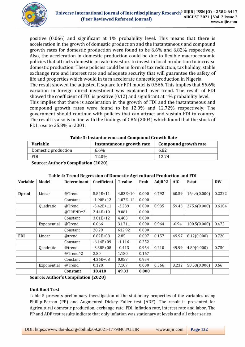
positive (0.066) and significant at 1% probability level. This means that there is acceleration in the growth of domestic production and the instantaneous and compound growth rates for domestic production were found to be 6.6% and 6.82% respectively. Also, the acceleration in domestic production could be due to flexible macroeconomic policies that attracts domestic private investors to invest in local production to increase domestic production. These policies could be in form of tax reduction, tax holiday, stable exchange rate and interest rate and adequate security that will guarantee the safety of life and properties which would in turn accelerate domestic production in Nigeria. The result showed the adjusted R square for FDI model is 0.566. This implies that 56.6% variation in foreign direct investment was explained over trend. The result of FDI showed the coefficient of FDI is positive (0.12) and significant at 1% probability level. This implies that there is acceleration in the growth of FDI and the instantaneous and compound growth rates were found to be 12.0% and 12.72% respectively. The government should continue with policies that can attract and sustain FDI to country. The result is also is in line with the findings of CBN (2004) which found that the stock of FDI rose to 25.8% in 2001.

Table 3: Instantaneous and Compound Growth Rate

Variable Instantaneous growth rate Compound growth rate

Domestic production 6.6% 6.82

FDI 12.0% 12.74


Table 4: Trend Regression of Domestic Agricultural Production and FDI

Variable Model Determinant Coefficient T-value Prob AdjR^2 AIC Fstat DW

Dprod Linear @Trend 5.84E+11 4.83E+10 0.000 0.792 60.59 164.4(0.000) 0.2222

Constant -1.90E+12 1.07E+12 0.000

Quadratic @Trend -3.42E+11 -3.239 0.000 0.935 59.45 275.6(0.000) 0.6104

@TREND^2 2.44E+10 9.081 0.000

Constant 3.81E+12 4.403 0.000

Exponential @Trend 0.066 31.711 0.000 0.964 -0.94 100.5(0.000) 0.472

Constant 28.29 612.92 0.000

FDI Linear @trend 6.82E+08 2.85 0.007 0.157 49.97 8.12(0.000) 0.720

Constant -6.14E+09 -1.116 0.252

Quadratic @trend -3.38E+08 -0.413 0.954 0.210 49.99 4.80(0.000) 0.750

@Trend^2 2.80 1.180 0.167

Constant 4.36E+08 0.057 0.954

Exponential @Trend 0.120 7.107 0.000 0.566 3.232 50.53(0.000) 0.66

Constant 18.418 49.33 0.000


Unit Root Test

Table 5 presents preliminary investigation of the stationary properties of the variables using

Phillip-Perron (PP) and Augmented Dickey–Fuller test (ADF). The result is presented for

Agricultural domestic production, exchange rate, FDI, inflation rate, interest rate and labor. The

PP and ADF test results indicate that only inflation was stationary at levels and all other series

© UIJIR | ISSN (O) – 2582-6417





Page 133

were not integrated at I(0) level but integrated of order I(1) or at first difference.

The result implies that level form of these series exhibited random walk or have multiple means

of covariance or both. However, the first difference of those variables is integrated or stationary.

The existence of difference in stationarity level form of the series necessitated bounds test after

the initial ARDL to examine long run causation or relationship in the variables. According to

Enger and Granger (1987), the linear combination of non-stationary variables is often co-

integrated.

In other to correct for the biasness in Philip-Perron and ADF statistics which could not account

for structural break in the model, Zivot and Andrew test that gives the potential break points of

each variable with their respective break point year was applied and it is presented in table 6.

Table 5: Unit Root Test for all Variables (PP and ADF)

Variables Phillip-Perron (PP) Augmented-Dickey Fuller (ADF)

At level Difference At level Difference

T-statistic T-statistic T-statistic Prob T-statistic Prob.

LnDPROD 0.9116 0.9946 0.9118 0.9946 -5.66400 0.000

LnEX__RATE -1.7161 0.4156 -1.7161 0.4153 -5.26858 0.000

LnFDI -1.8260 0.3627 -1.8260 0.3627 -5.03818 0.000

LnINF_RATE -3.9288 0.000 -3.9284 0.0045

LnINT_RATE -2.2795 0.1835 -2.2795 0.1835 -6.57544 0.0000

LnLABOUR -2.333 .09988 -2.3321 0.9999 -6.4093 0.000

*** denotes rejection of the null hypothesis at 1 percent level of significance

NOTE: EX_RATE= exchange rate, INF_RATE= inflation rate DPROD = domestic production


Table 6: Unit Root Test for all Variables using Zivot and Andrew Test

Level First Difference

Variables t-statistic Break Year t-statistic Break Year

LnDPROD -3.4349 2001 -5.236 2005

LnEX_RATE -2.5881 1989 4.9921 2002

LnFDI 2.8788 2001 3.9961 2005

LnINF_RATE -3.1156 1999 -4.1231 1990

LnINT_RATE -2.5872 1999 -3.6112 1990

LnLABOUR -5.2314 2002 -6.0142 2005


Lag Length Selection Criteria

Table 7 presents the result of lag length from six different selection criteria to ascertain the

optimum lag for the ARDL model. The model showed that the optimum lag is 1; Akaike

Information Criterion was chosen because of its lowest value 3.951 at lag 1. Lag 1 is the

appropriate lag to be in used for the model.

Table 7: Lag length of the Model

Lag LogL LR FPE AIC SC HQ

© UIJIR | ISSN (O) – 2582-6417





Page 134

0 -226.2973 NA 0.008221 12.22618 12.48474 12.31817

1 -33.07713 315.2540* 4.15e-06* 3.951428* 5.761392* 4.595399*

* indicates lag order selected by the criterion

LR: sequential modified LR test statistic (each test at 5% level)

FPE: Final prediction error

AIC: Akaike information criterion

SC: Schwarz information criterion

HQ: Hannan-Quinn information criterion


• Bounds Test

Table 8 present the result of bounds co-integration test that shows how long its relations exist

among log of variables used in the model from initial ARDL, the F statistics value of

5.33(0.000) greater than the critical value of the I1 bound value of 4.68 at 1% probability

levels, showing it’s long run relations that exist among variables and this necessitated the long

form of ARDL for co-integration.

Table 8: Bounds Test for co-integration

Null Hypothesis: No long-run relationships exist

Test Statistic Value K

F-statistic

5.390513136

553523 5

Critical Value Bounds

Significance I0 Bound I1 Bound

10% 2.26 3.35

5% 2.62 3.79

2.5% 2.96 4.18

1% 3.41 4.68

• Short and Long Run Impact of FDI on Domestic Agricultural Production Using ARDL

Model Based on AIC

Table 9 shows the result of estimated ARDL. Indicating adjusted R-square of 0.994, this means that 99.4% variation in the log of domestic production is explained by the explanatory variables used in the model. The short run model is known as the cointegrating form of ARDL model. The cointegration equation shows negative (-0.303) with 1% significant level of probability. This means that the system has a self-adjustment mechanism with a speed of adjustment of 30.03% which implies that previous year’s error is corrected in current year or any disequilibrium in the short run will be corrected at the highest speed of 30.03% in the long run annually which allows the model to return to equilibrium. In the short run, log of FDI was positive and significant at 5% significant levels. Meaning an increase in log of FDI will increase log of domestic production by the value of its coefficient. The log of labor is positive (0.03) and it is significant at 1% probability level, implying that an increase in the log of labour increase log of domestic production in

© UIJIR | ISSN (O) – 2582-6417





Page 135

Nigeria by the value of its coefficient. All other variables used in the model are positive and not significant. In the long run, the coefficient of log of exchange rate, interest rate and labor are positive and significant at 1% probability level. This means acceleration in the log of these variables will lead to acceleration in the log of domestic production with the value of their coefficients. The coefficient of FDI is positive and significant at 5% significant level, this also implies that acceleration in the log of FDI will lead to acceleration in the log of domestic production in Nigeria. The coefficient of inflation rate is positive and not significant. Increase in domestic production per unit increase in FDI could be due to attractive macroeconomic fiscal and monetary policies such as tax reduction, stabilization of exchange and interest rate and increase in government spending on basic social amenities including electricity, roads, health center, pipe borne water etc. Increase in FDI means increase in the nation’s gross capital formation, increase in economic activities as well as increase in labour involve in agricultural production. Similarly, to the outcome of Adeleke et al. (2014) observed an increase in FDI increases GDP in Nigeria. The finding is also in consonant with Otepola (2002) who found that FDI contributes significantly to growth especially through exports.

Table 9: Cointegration and Long Run Form

ARDL Cointegrating And Long Run Form

Dependent Variable: SER01

Cointegrating Form (Short Run)

Variable Coefficient Std. Error t-Statistic Prob.

D(Ex_rate) -0.000757 0.043919 -0.017237 0.9864

D(FDI) 0.042239 0.016088 2.625385 0.0244

D(INFL) 0.013535 0.018574 0.728706 0.4722

D(INT) -0.050935 0.094209 -0.540656 0.5930

D(LAB) 0.030563 0.010589 2.886162 0.0074

CointEq(-1) -0.303824 0.082003 -3.705022 0.0009

Long Run Coefficients

Variable Coefficient Std. Error t-Statistic Prob.

EX_rate 0.443016 0.054011 8.202328 0.0000

FDI 0.023263 0.041445 -0.561301 0.0271

Infl_rate 0.044550 0.062274 0.715377 0.4803

Intr_rate -1.024496 0.208599 -4.911314 0.0000

Labour 0.100594 0.022444 4.481939 0.0001

C 29.751826 1.256119 23.685507 0.0000

© UIJIR | ISSN (O) – 2582-6417





Page 136

R-squared 0.994124 Mean dependent var 29.58557

Adjusted R-squared 0.992235 S.D. dependent var 0.760835

S.E. of regression 0.067045 Akaike info criterion -2.345956

Sum squared resid 0.125863 Schwarz criterion -1.915013

Log likelihood 54.57317 Hannan-Quinn criter. -2.192630

F-statistic 526.3096 Durbin-Watson stat 2.018124

Prob(F-statistic) 0.000000

*Note: p-values and any subsequent tests do not account for model

selection.


• Causal relationship between Domestic Agricultural Production and FDI

The result of the causal relationship between domestic production and FDI is presented in

table 10 below. This indicates unidirectional causal relationship between domestic production

and FDI. But FDI does not Granger cause domestic production. This implies that the past

value of domestic production may have influence on future value of FDI. This is in line with

Udousoro et. al. (2013) who found a unidirectional causality between and foreign capital

investment and exchange rate but foreign capital does not Granger cause exchange rate.

Table 10: Granger Causality Tests

Null Hypothesis F-Statistics Prob.

Ln Ex_rate does not Granger Cause LnDProd 2.03804 0.1623

LnDProd does not Granger Cause LnEx_rate 0.01527 0.9024

LnFDI does not Granger Cause LnDProd 0.46090 0.5017

LnDProd does not Granger Cause LnFDI 3.18901 0.0328

LNInfl_rate does not Granger Cause LnDProd 0.05333 0.8187

LnDProd does not Granger Cause LnInfl_rate 0.71134 0.4047

LnInt_rate does not Granger Cause LnDProd 0.07107 0.7914

LnDProd does not Granger Cause LnInt_rate 0.05575 0.8147

LnLab does not Granger Cause LnDprod 0.00393 0.9504

LnDprod does not Granger Cause LnLab 1.75119 0.1943

LnFDI does not Granger Cause LnEx_rate 0.01900 0.8912

LnEx_rate does not Granger Cause LnFDI 3.80950 0.0590

LnInfl_rate does not Granger Cause LnEx_rate 0.57803 0.4522

LnEx_rate does not Granger Cause LnInfl_rate 0.18889 0.6665

LnInt_rate does not Granger Cause LnEx_rate 0.03947 0.8437

LnEx_rate does not Granger Cause LnInt_rate 0.41672 0.5228

LnLab does not Granger Cause LnEx_rate 0.00689 0.9343

LnEx_rate does not Granger Cause LnLab 0.63299 0.4316

LnInfl_rate does not Granger Cause LnFDI 0.09088 0.7649

LnFDI does not Granger Cause LnInfl_rate 0.64475 0.4274

LnInt_rate does not Granger Cause LnFDI 3.91009 0.0559

LnFDI does not Granger Cause LnInt_rate 0.01468 0.9042

LnLab does not Granger Cause LnFDI 2.19155 0.1477

LnFDI does not Granger Cause LnLab 2.64894 0.1126

LnInt_rate does not Granger Cause LnInfl_rate 0.74943 0.3926

LnInfl_rate does not Granger Cause LnInt_rate 1.33209 0.2563

LnLab does not Granger Cause LnInfl_rate 0.00518 0.9430

© UIJIR | ISSN (O) – 2582-6417





7

LnInfl_rate does not Granger Cause LnLab 0.02763 0.8689

LnLab does not Granger Cause LnInt_rate 0.11154 0.7404

LnInt_rate does not Granger Cause LnLab 0.65564 0.4236


CONCLUSION

The research determined how foreign direct investment has influence domestic agricultural

production in Nigeria. With different order of stationarity, a bounds test approach embedded in

the ARDL was carried out confirming a long run relationship among all the variables. The study

revealed acceleration in growth of domestic production and FDI. Only FDI and labor had

significant effect on domestic production in short run and all variables in the model except

inflation rate had impact on domestic production in the long run.The results revealed past values

of domestic agricultural production can predict the future value of FDI. The positive impact of FDI

on domestic agricultural production both in the short and long run suggests that Nigeria

government should make policies that can lead to increased inflows of FDI to domestic production

so that domestic production can meet its capacity demand. Macroeconomic policies that will

strengthen the naira value and reduce interest rate for farm purposes which suggests labour

availability and stability of exchange rate as it tend to affect domestic agricultural production.

The study is limited to 38 years because of availability of data. Future studies should be on

individual domestic agricultural production subsector like crop, fishery, livestock and forestry to

know the impact of FDI on these subsectors. Also, future studies should give apriority to influence

of private investment on domestic production.

REFERENCES

• Adeleke K. M., Olowe S. O. & Fasesin O. O. (2014). Impact of Foreign Direct Investment on

Nigeria Economic Growth. International Journal of Academic Research in Business and Social

Sciences ,4(8):234-242.

• Agba, D. Z., Adewara, S. O., Nwanji, T., Yusuf, M., Adzer, K. T. & Abbah, B. (2018). Does Foreign

Direct Investements impact Agricultural Output in Nigeria? An Error correction Modelling

Approach. Journal of Economics and Sustainable Development, 9(4):67-77.

• Akpan, S. B., Edet, U. J., & Umoren, A. A. (2012). Modeling the dynamic relationship between food

crop output volatility and its determinants in Nigeria. Journal of Agricultural Science, 4(8), 36-

47. doi.org/10.5539/jas.v4n8p36

• Ake, C. (1996). Democracy and Development in Africa. Brookings Institution, Washington DC,

184pp.

• Akinwale, S. O., Adekunle, E. O. & Obagunwa, T. B. (2018). Foreign Derict Investment Inflow in

Agricultural Sector Productivity in Nigeria. Journal of Economics and Finance, 9(4):12-19.

• Apter, D. E. (1965). The Politics of Modernization. The University of Chicago Press, Chicago. Pp.

Xii, 481.

• Aremu, J. A. (1997), “Foreign Private Investment: Issues, Determinants and Performance”, Paper

presented at a workshop on foreign investment policy and practice, organized by the Nigeria

Institute of Advance Legal Studies, Lagos, Nigeria.

• Awunyo-Vitor, D. & Sackey, R. A. (2018). Agricultural sector foreign direct investment and

economic growth in Ghana. Journal of Innovation and Entrepreneurship, 7(15):1-15.

https://doi.org/10.1186/s13731-018-0094-3.

• Bailey, R. (1995). Governing the Workplace. British Journal of Industrial Relations, 33(4):557-

https://doi.org/10.1186/s13731-018-0094-3

© UIJIR | ISSN (O) – 2582-6417





Page 138

562.

• Binuyo, B. O. (2014). Impact of Foreign Direct Investment on Agricultural Sector Development in

Nigeria, 1981-2012. Kuwait Chapter of Arabian Journal of Business and Management Review,

3(12):14-24.

• Central Bank of Nigeria (CBN) (2004). Annual Report and Statement of Account, Abuja, Nigeria.

CIA (2020). The World Fact Book. Accessed 3 December, 2020, from

https://www.cia.gov/library/publications/the-world-factbook/geos/ni.html

• Dickey, D. A., & Fuller, W. A. (1981). Likelihood ratio statistics for autoregressive time series

with a unit root. Econometrica: Journal of the Econometric Society, 49, 1057–1072.

• Dunning, J. H. & Sarianna,M. L. (2008). Multinational Enterprises and the Global Economy.

Edward Elgar Publishing.

• Edet J. U. & Akpan, S. B. (2019). Macroeconomic variables affecting fish production in Nigeria.

Asian Journal of Agriculture and Rural Development, 9(2), 216-230.

• Edewor, S. U., Dipeolu, A. O., Ashaolu, O. F., Akinbode, S. O., Ogbe, A. O., Edewor, A. O., Tolorunju,

E. T. & Oladeji, S. O. (2018). Contribution of Foreign Direct Investment and other Selected

Variables to Agricultural Productivity in Nigeria: 1990-2016. Nigerian Journal of Agricultural

Economics, 8(1):50-61.

• Enger, R. F. & Granger, C. W. J. (1987). Co-integration and Error Correction: Representation,

Estimation and Testing. Econometrica, 55(2):251-276

• Falki, N. (2009) Impact of Foreign Direct Investment on Economic Growth in Pakistan. Review of

Business Research Papers, Vol. 5 No. 5.

• Fischer, S. and Gelb, A. (1991). The Process of Socialist Economic Transformation. The Journal of

Economic Perspectives, 5(4):91-105.

• Iddrisu, A., Immrana, M. & Halidu, B. O. (2015). The impact of Foreign Direct Investment on the

performance of the Agricultural Sector in Ghana. International Journal of Academic Research in

Business and Social Sciences, 5(7):240-259.

• Kareem, R., Bakara, H., Raheem, K., Ologunla, S., Alawode, O. & Ademoyewa, G. (2013). Analysis

of factors influencing agricultural output in Nigeria: macro-economic perspectives. Am. J. Bus.

Econ. Manag, 1:9-15.

• Meo, M. S., Khan, V. J., Ibrahim, T. O., Khan, S., Ali, S., & Noor, K. (2018). Asymmetric impact of

inflation and unemployment on poverty in Pakistan: New evidence from asymmetric ARDL

cointegration. Asia Pacific Journal of Social Work and Development, 28(4), 295–310.

• Meo, M., Nathaniel, S., Shaikh, G., & Kumar, A. (2020). Energy consumption, institutional quality

and tourist arrival in Pakistan: Is the nexus (a)symmetric amidst structural breaks? Journal of

Public Affairs. https://doi.org/10.1002/pa.2213

• Msuya, E. (2007). The Impact of Foreign Direct Investment on Agricultural Productivity and

Poverty Reduction in Tanzania. MPRA Paper No. 3671, http://mpra.ub.uni-muenchen.de/3671/

• Nchuchume, F. F., & Adejuwon, K. D. (2012). The challenge of agriculture and rural development

in Africa: The case study of Nigeria. International Journal of Academic Research in Progressive

Education and Development, 1(3):45-61.

• OECD (2008).“Main Concepts and Definitions of Foreign Direct Investment”. OECD Benchmark

Definition of Foreign Direct Investment. Fourth Edition. OECD Publishing, Paris. DOI:

https://doi.org/10.1787/9789264045743-5-en

• Oluwatoyese, O. P., Applanaidu, S. D., & Razak, N. A. A. (2016). Macroeconomic Factors and

Agricultural Sector in Nigeria. Procedia - Social and Behavioral Sciences, 219, 562–570.

https://doi.org/10.1016/j.sbspro.2016.05.035

https://www.cia.gov/library/publications/the-world-factbook/geos/ni.html

https://doi.org/10.1002/pa.2213

http://mpra.ub.uni-muenchen.de/3671/

https://doi.org/10.1787/9789264045743-5-en

https://doi.org/10.1016/j.sbspro.2016.05.035

© UIJIR | ISSN (O) – 2582-6417





Page 139

Oloyede, B.B. (2014). Impact of foreign direct investment on agricultural sector development in

Nigeria, (1981-2012). Kuwait Chap Arab J Bus Manag Rev, 3(12):14

• Otepola, A. (2002): “FDI as a Factor of Economic Growth in Nigeria. Dakar, Senegal”. African

Institute for Economic Development and Planning (IDEP), May. Available online at:

[email protected], http://www.unidep.org.

• Oyinbo, O. & Rekwot, G.Z. (2013). Fishery production and economic growth in Nigeria. Journal of

Sustainable Development in Africa, (15): 1520-5509.

• Phillips, P. C., & Perron, P. (1988). Testing for a unit root in time series regression. Biometrika,

75(2), 335–346.

• Udousoro, E. E., Eko, A. S. & Ubong, U. (2013). Dynamic Analysis of Savings and Economic

Growth in Nigeria. Journal of Agriculture and social science. 13(2):9-15.

• Umechukwu, J. N. & Okezie, C. A. (2018). Impact of Foreign Direct Investment on Nigerian

Agricultural Sector, 1970-2014. International Journal of Applied Research and Technology,

7(8):8-15.

• Wiggins, S., Farrington, J., Henley, G., Grist, N., & Anne, L. (2013). Agricultural Development

policy: A comtemporary agenda background paper for GIZ. Overseas Development Institute, UK.

Pp1-142.

• Zivot, E., & Andrews, D. W. K. (1992). Further evidence on the great crash, the oil price shock,

and the unit root hypothesis. Journal of Business and Economic Statistics, 10(3), 251–270.

APPENDIX

DIGNOSTIC CHECKING

Stability Test

Figure 1 presents the result for structural break of the model using the CUSUM test. The CUSUM

test line is situated between the gridlines, this implies that it lies between two standard

deviation or 95% confident interval level. From the graphs it showed that there is no break, all

residuals are stable since it is maintained within the 5% significant level during the period of

observation and the model is said to be a fitted model.

-20

-15

-10

-5

0

5

10

15

20

10 15 20 25 30 35

CUSUM 5% Significance Figure1: Stability Test

LM TEST FOR SERIAL CORRELATION

The LM for serial correlation is presented in the table below. The result of LM test confirm the

http://www.unidep.org/

© UIJIR | ISSN (O) – 2582-6417





Page 140

Durbin Watson statistics value of 2.018 which means variable are free autocorrelation. The

Breuch-Godfrey LM test for serial for correlation shows the probability value of 0.5885, this is

insignificant at 5% significant level. This implies model is free from autocorrelation.

Breusch-Godfrey Serial Correlation LM Test:

F-statistic 0.541194 Prob. F(2,26) 0.5885

Obs*R-squared 1.518726 Prob. Chi-Square(2) 0.4680


HETEROSKEDASTICITY TEST

Table present the result of heteroskedasticity below. The test suggest variable are free from the

problem of heteroskedasticity since probability value and Obs*R-square of 0.0635 and 0.0598

are greater than 5%.

Heteroskedasticity Test: Breusch-Pagan-Godfrey

F-statistic 2.950340 Prob. F(9,28) 0.0635

Obs*R-squared 18.49605 Prob. Chi-Square(9) 0.0598

Scaled explained SS 17.48249 Prob. Chi-Square(9) 0.0417


NORMALITY TEST

The figure 2 below presented the graph of normality test. The result showed it is positively

skewed to right tail and kurtosis greater than 3 meaning it is leptokurtic under the null

hypothesis of that residual are normally distributed. The Jarque-Berra test probability value

0.0011 showed the null hypothesis can be accepted that the residual are normally distributed.

0

2

4

6

8

10

12

-0.10 -0.05 0.00 0.05 0.10 0.15 0.20

Series: ResidualsSample 2 39Observations 38

Mean -7.94e-16Median -0.009553Maximum 0.190359Minimum -0.111157Std. Dev. 0.058324Skewness 0.934284Kurtosis 4.481812

Jarque-Bera 9.004912Probability 0.011082

Figure 2: Normality Test

COLLELOGRAM TEST FOR AUTO CORRELATION

The table below presents the collelogram test for autocorrelation. The Q statistics suggests

variable are free from autocorrelation with probality value greater than 5%.

© UIJIR | ISSN (O) – 2582-6417





Page 141

Autocorrelation Partial Correlation AC PAC Q-Stat Prob*

. | . | . | . | 1 -

0.039

-

0.039

0.0633 0.801

.*| . | .*| . | 2 -

0.162

-

0.164

1.1774 0.555

. | . | . | . | 3 0.071 0.058 1.3937 0.707

.*| . | .*| . | 4 -

0.176

-

0.204

2.7824 0.595

.*| . | .*| . | 5 -

0.174

-

0.177

4.1706 0.525

. | . | . | . | 6 0.065 -

0.022

4.3711 0.627

. | . | . | . | 7 0.000 -

0.045

4.3711 0.736

. | . | .*| . | 8 -

0.051

-

0.074

4.5014 0.809

. | . | . | . | 9 0.049 -

0.038

4.6276 0.865

. | . | . | . | 1

0

0.066 0.027 4.8667 0.900

. | . | . | . | 1

1

0.052 0.071 5.0195 0.930

.*| . | .*| . | 1

2

-

0.163

-

0.188

6.5790 0.884

.*| . | .*| . | 1

3

-

0.080

-

0.110

6.9715 0.904

. | . | . | . | 1

4

0.056 0.006 7.1672 0.928

.*| . | .*| . | 1

5

-

0.136

-

0.141

8.3973 0.907

. |*. | . | . | 1

6

0.100 0.049 9.0856 0.910

*Probabilities may not be valid for this equation specification.

IMPACT OF FOREIGN DIRECT INVESTMENT(FDI) ON DOMESTIC ...

Documents

Transcript of IMPACT OF FOREIGN DIRECT INVESTMENT(FDI) ON DOMESTIC ...