This is an electronic reprint of the original article.This reprint may differ from the original in pagination and typographic detail.

Powered by TCPDF (www.tcpdf.org)

This material is protected by copyright and other intellectual property rights, and duplication or sale of all or part of any of the repository collections is not permitted, except that material may be duplicated by you for your research use or educational purposes in electronic or print form. You must obtain permission for any other use. Electronic or print copies may not be offered, whether for sale or otherwise to anyone who is not an authorised user.

Deb, Sanchari; Tammi, Kari; Kalita, Karuna; Mahanta, PinakeshwarImpact of Electric Vehicle Charging Station Load on Distribution Network

Published in:Energies

DOI:10.3390/en11010178

Published: 15/01/2018

Document VersionPublisher's PDF, also known as Version of record

Please cite the original version:Deb, S., Tammi, K., Kalita, K., & Mahanta, P. (2018). Impact of Electric Vehicle Charging Station Load onDistribution Network. Energies, 11(1), [en11010178]. https://doi.org/10.3390/en11010178

energies

Article

Impact of Electric Vehicle Charging Station Load onDistribution Network

Sanchari Deb 1,*, Kari Tammi 2,* ID , Karuna Kalita 3 ID and Pinakeshwar Mahanta 3

1 Centre for Energy, Indian Institute of Technology, Guwahati 781039, Assam, India2 Department of Mechanical Engineering, Aalto University, 02150 Espoo, Finland3 Department of Mechanical Engineering, Indian Institute of Technology, Guwahati 781039, Assam, India;

karuna.kalita@iitg.ernet.in (K.K.); pinak@iitg.ernet.in (P.M.)* Correspondence: sancharideb@yahoo.co.in (S.D.); kari.tammi@aalto.fi (K.T.)

Received: 19 November 2017; Accepted: 20 December 2017; Published: 15 January 2018

Abstract: Recent concerns about environmental pollution and escalating energy consumptionaccompanied by the advancements in battery technology have initiated the electrification of thetransportation sector. With the universal resurgence of Electric Vehicles (EVs) the adverse impactof the EV charging loads on the operating parameters of the power system has been noticed.The detrimental impact of EV charging station loads on the electricity distribution network cannotbe neglected. The high charging loads of the fast charging stations results in increased peak loaddemand, reduced reserve margins, voltage instability, and reliability problems. Further, the penaltypaid by the utility for the degrading performance of the power system cannot be neglected. This workaims to investigate the impact of the EV charging station loads on the voltage stability, power losses,reliability indices, as well as economic losses of the distribution network. The entire analysis isperformed on the IEEE 33 bus test system representing a standard radial distribution network forsix different cases of EV charging station placement. It is observed that the system can withstandplacement of fast charging stations at the strong buses up to a certain level, but the placement offast charging stations at the weak buses of the system hampers the smooth operation of the powersystem. Further, a strategy for the placement of the EV charging stations on the distribution networkis proposed based on a novel Voltage stability, Reliability, and Power loss (VRP) index. The resultsobtained indicate the efficacy of the VRP index.

Keywords: charging station; distribution network; power loss; reliability; voltage stability

1. Introduction

The perpetually escalating demands for energy and the finite nature of the fossil fuel supply,accompanied by global warming and climate change are the main concerns of environmentalists andresearchers in the 21st century. The CO2 emissions from the transportation sector are one of the maincauses of global warming and climate change [1–3]. Researchers have stressed the positive impact ofreplacing Internal Combustion Engine (ICE) driven vehicles with Electric Vehicles (EVs) to minimizethe greenhouse gas contributions of the transport sector. The paradigm shift from conventional vehiclesto EVs has many environmental and economic advantages. The increasing number of EVs is howeveraccompanied by a rise in charging demand. Hence, the development of the charging infrastructure aswell as efficient Inductive Power Transfer (IPT) [4] has become necessary to meet the requirementsof substantial operation of the EVs [5]. For instance, in the United States (US), the National ProgramCharging Point America has taken an initiative of building nearly 5000 EV charging stations to offercharging services in nine regions of the U.S. [6]. Even a developing country like Bhutan has takenan initiative to set up charging infrastructure for the promotion of the EVs [7]. The establishment ofcharging stations imposes an additional burden on the power grid, as the high charging loads of fast EV

Energies 2018, 11, 178; doi:10.3390/en11010178 www.mdpi.com/journal/energies

Energies 2018, 11, 178 2 of 25

charging stations will degrade the operating parameters of the distribution network. The degradationof voltage profile, increase in peak load, harmonic distortions are some of the consequences of theuncoordinated charging of EVs. Many references demonstrate the adverse impact of EV chargingloads on different parameters of the distribution network like voltage profile [8–14], harmonics [15–18]and peak load [19–24].

The potential impact of EV charging station loads on the voltage profile of distribution networkshas been investigated by a number of researchers. In [8] the authors analysed the impact of the EVcharging station loads on a low voltage distribution network in Europe for different EV penetrationscenarios. It was concluded in [8] that the network was robust enough to support a low intake ofEVs 1–2%. However, it was observed that the voltage profile of the node where multiple chargingstations were placed degraded to some extent and the high loads of EV charging stations causeddegradation of the voltage profile of the weak buses of the system. In [9] the authors examined theimpact of EV charging loads on a 13 node distribution network for different EV penetration scenarios.In [10] the authors analysed the impact of EV charging loads on a standard distribution network with14 buses. It was concluded that the transient voltage stability index degraded for high penetrationof EVs. The impact of EV charging loads on the voltage stability of distribution network was alsoanalysed in [11–14]. From the findings of [11–14], it is observed that most of the distribution networkscould withstand the penetration of EVs up to a certain level. However, networks designed a decadeago are not equipped to withstand any large-scale integration of EVs.

Harmonics being a crucial outcome of EV integration have been analysed in depth by researchersin recent years. In [15] the authors investigated the effect of EV charging loads on the harmonic voltagesof distribution system by applying statistical analysis. The authors classified the chargers based on thetotal harmonic distortion (THDI) produced and concluded that even with 45% EV penetration therewas negligible harmonic distortion during summer. The effect of non-linear EV charging loads onpower quality of the distribution system was analysed in [16], where it was reported that the lifecycleof distribution network assets was reduced by the harmonic distortion produced by the EV loads.In [17] the authors reported that the EV battery charging loads caused harmonic distortion of even50% in the most extreme cases. In [18] the authors simulated the harmonics caused by Plug-in HybridElectric Vehicle (PHEV) chargers by a probabilistic Monte Carlo approach considering the uncertainties.It was concluded that residential Level 1 chargers (1.8 kW) had a severe impact on the power quality.

In recent years researchers have concentrated on quantifying the variation of peak load demandafter the placement of EV charging stations in the distribution network. In [19] the authors examinedthe effect of the PHEV loads on the metropolitan distribution network of Australia, concluding thatwith uncoordinated charging and 100% PEV penetration 43% peak load shifting was required to enablesmooth operation of the distribution network. In [20] the authors analysed the effect of the uncontrolledEV charging on the daily load profile. The improvement in load profile by incorporating coordinatedcharging was also illustrated in [20]. In [21] the authors concluded that disorderly charging wouldincrease the peak load demand and recommended tariff based charging. In [22] the authors analysedthe impact of EV charging on daily load demand in the parking lots and devised an optimal strategyfor controlling the charging activities in the parking lots. In [23] the authors analysed the impact of fastEV chargers on a retail building’s load demand and concluded that 38% of the PHEV load demandcould be absorbed by demand management and photovoltaics. In [24] the authors proposed a twostage demand response model to control the increase in peak load due to the charging of EVs.

The different detrimental impacts of EV charging station loads like voltage instability, harmonicdistortion, and power losses on distribution network are analysed in [8–24]. However, there is adearth of literature focusing on the impact of the EV charging station load on all the aforementionedparameters considered together. The analysis is usually performed for one or two parameters separately.All the aforementioned limitations of the existing literature are addressed in this work and the majorcontributions of the work are summarized as follows:

Energies 2018, 11, 178 3 of 25

• Profound analysis of the impact of the EV charging station loads on the voltage stability of thedistribution network.

• Detailed analysis of the impact of the EV charging station loads on the customer and energyoriented reliability indices.

• Comprehensive analysis of the economic losses incurred in terms of the penalty paid by the utilitydue to introduction of the EV charging station loads.

• Comparative analysis of the EV charging load on different parameters of the distribution networksuch as the voltage stability, reliability and power losses.

• Placement of the charging stations in the distribution network based on VRP index.

The rest of the paper is organized as follows: Section 2 illustrates the computational methodologyof voltage stability, reliability, power loss, and economic loss. Section 3 demonstrates the mathematicalformulation of VRP index and the problem formulation for the optimal placement of the chargingstations based on VRP index. Section 4 presents the results of the impact of the charging station load onthe distribution network as well as the optimal locations of the charging stations in the IEEE 33 bus testnetwork. Section 5 presents a brief discussion on the findings of the work. Finally, Section 6 concludesthe work.

2. Methodology

The voltage stability, reliability, and power losses are the three important operational parametersof the distribution network. A brief overview of the methodology to compute voltage stability,reliability, power losses, and economic loss of the distribution network is elaborated in this section.Further, the overall computational methodology adopted for analysing the impact of EV chargingstation load on distribution network is also presented in this section.

2.1. Voltage Stability

The voltage stability problem has concerned power system engineers for many years. Voltagestability is the power system’s capability to maintain steady acceptable voltages at all the system busesunder normal operating conditions and when an external disturbance is applied [25,26]. During voltageinstability phenomena, the bus voltage of the network declines progressively and uncontrollably.The system may become unstable because of sudden disturbances, fault conditions, single or multiplecontingencies, line overloading or load increases. A voltage stability criterion used in many stabilitystudies is that voltage of all the system buses must be within acceptable limits. Voltage stability isindeed a local phenomenon but in some cases, it may lead to severe voltage collapse [25]. In this workVoltage Sensitivity Factor (VSF), Voltage Stability Index (VSI) are used for voltage stability analysis.

2.1.1. Voltage Sensitivity Factor

Voltage stability studies generally obey a static approach as the factors affecting it are slow innature. The voltage stability is analysed based on the determination of VSF from the PV curve [25,27,28].The PV curve is a graphical representation of active power and voltage [25]. It signifies the trend ofvoltage change with increasing active power as shown in Figure 1.

The first step for drawing the PV curve is the determination of the voltage of all the buses ofthe distribution network. For determination of voltage of a radial distribution network, the typicalmethods of load flow analysis like the Newton Raphson method have their limitations because of highR/X ratio. The R/X ratio is quite predominant in distribution system compared to transmission systemdue to low inductance of the line The Jacobian matrix may become singular because of high R/X ratio.Hence, the voltage of the buses is determined by the forward and backward sweep algorithm [29].From the PV curve shown in Figure 1 it is clear that as the active power increases, the voltage decreasesup to a point where the active power is highest (Pmax, Vcritical). That point corresponds to the critical

Energies 2018, 11, 178 4 of 25

operating condition known as the limit of stable operation. VSF is the ratio of change in voltage andchange in loading. Mathematically, it is expressed as:

VSF =

∣∣∣∣dVdP

∣∣∣∣ ∀ P < Pmax (1)

Energies 2018, 11, 178 4 of 25

corresponds to the critical operating condition known as the limit of stable operation. VSF is the ratio of change in voltage and change in loading. Mathematically, it is expressed as:

maxVSF dV P PdP

= ∀ < (1)

Figure 1. Active Power Voltage Curve (PV curve).

A high VSF value indicates that even for a small change in loading, there is a considerable voltage drop, thereby signifying weakness of the bus [28]. In voltage stability analysis of distribution networks, the voltage of all the buses must be within an acceptable limit (6% of their nominal value). The VSFs of all the buses are determined for increasing loading factor. The loading for which the voltages of all the buses are within acceptable range is called the realistic loading margin of the system [28]. The flowchart illustrating the methodology of computation of VSF is shown in Figure 2.

Figure 2. Flowchart for computation of VSF.

Calculate VSF for allbuses by Equation (1)

Start

Select the test system Input Bus and Line Data

Run distribution load flow for base case by forward backward method

Compute critical loading margin of the system and draw PV curve

Increase real load in steps

Run distribution load flow

Calculate VSF for all buses by Equation (1)

Load FlowConverge

Yes

No

End

Figure 1. Active Power Voltage Curve (PV curve).

A high VSF value indicates that even for a small change in loading, there is a considerable voltagedrop, thereby signifying weakness of the bus [28]. In voltage stability analysis of distribution networks,the voltage of all the buses must be within an acceptable limit (6% of their nominal value). The VSFsof all the buses are determined for increasing loading factor. The loading for which the voltagesof all the buses are within acceptable range is called the realistic loading margin of the system [28].The flowchart illustrating the methodology of computation of VSF is shown in Figure 2.

Energies 2018, 11, 178 4 of 25

corresponds to the critical operating condition known as the limit of stable operation. VSF is the ratio of change in voltage and change in loading. Mathematically, it is expressed as:

maxVSF dV P PdP

= ∀ < (1)

Figure 1. Active Power Voltage Curve (PV curve).

A high VSF value indicates that even for a small change in loading, there is a considerable voltage drop, thereby signifying weakness of the bus [28]. In voltage stability analysis of distribution networks, the voltage of all the buses must be within an acceptable limit (6% of their nominal value). The VSFs of all the buses are determined for increasing loading factor. The loading for which the voltages of all the buses are within acceptable range is called the realistic loading margin of the system [28]. The flowchart illustrating the methodology of computation of VSF is shown in Figure 2.

Figure 2. Flowchart for computation of VSF.

Calculate VSF for allbuses by Equation (1)

Start

Select the test system Input Bus and Line Data

Run distribution load flow for base case by forward backward method

Compute critical loading margin of the system and draw PV curve

Increase real load in steps

Run distribution load flow

Calculate VSF for all buses by Equation (1)

Load FlowConverge

Yes

No

End

Figure 2. Flowchart for computation of VSF.

Energies 2018, 11, 178 5 of 25

2.1.2. Bus Voltage Stability Index

The voltage stability index developed by Eminoglu et al. [30] is utilized in this work. The mathematicalformulation of the index is illustrated by taking an example of a simple 2 bus system as shown inFigure 3. The mathematical formulation of this index is elaborated by Equation (2) to Equation (8).

Energies 2018, 11, 178 5 of 25

2.1.2. Bus Voltage Stability Index

The voltage stability index developed by Eminoglu et al. [30] is utilized in this work. The mathematical formulation of the index is illustrated by taking an example of a simple 2 bus system as shown in Figure 3. The mathematical formulation of this index is elaborated by Equation (2) to Equation (8).

Figure 3. Single line diagram of a simple two bus system.

Figure 3 illustrates the single line diagram of a two bus system where j and j + 1 are the two buses of the system. Vj < δj and Vj+1 < δj+1 are the voltage at bus j and bus j + 1 respectively. I is the current flowing through the branch having resistance r and impedance x:

xrVV

I jj

i1

+−

= + (2)

IVQP jjj*

111 i +++ =− (3)

Substituting value of I in Equation (3), equating real parts and on further simplification Equation (4) is obtained:

0)()(2 221

21

21

211

21

41 =++−++ +++++++ ZQPVVxQrPVV jjjjjjjj (4)

From Equation (4) the transferrable active and reactive power can be written as in Equation (5) and Equation (6), respectively:

ZNMPj

±=+1 (5)

where

21cos +−= jzVM θ, and

2

12

12

12

124

14

12 2cos ++++++ +−−−= jjjjjjjz VVxQVQZVVN θ

.

ZQP

Qj±

=+1 (6)

where: 21sin +−= jzVP θ,

and:

21

21

21

21

241

41

2 2sin ++++++ +−−−= jjjjjjjz VVrPVPZVVQ θ.

Thus, the conditions of existence of transferrable active and reactive power are as in Equation (7):

≥ ≥0 and 0N Q (7)

Substituting the actual values of N, Q and adding them leads to the inequality defining the stability criterion of the system:

0)()(22 21

21

211

21

21

2 ≥+−+− ++++++ jjjjjjj QPZxQrPVVV (8)

The value of Equation (8) is known as VSI. This is a criterion for determination of voltage stability. VSI will decrease with increase of active power. Increasing the active power beyond a certain limit will cause the system to become unstable. The flowchart illustrating the methodology of computation of VSI is shown in Figure 4.

Figure 3. Single line diagram of a simple two bus system.

Figure 3 illustrates the single line diagram of a two bus system where j and j + 1 are the two busesof the system. Vj < δj and Vj+1 < δj+1 are the voltage at bus j and bus j + 1 respectively. I is the currentflowing through the branch having resistance r and impedance x:

I =Vj −Vj+1

r + ix(2)

Pj+1 − iQj+1 = V∗j+1 I (3)

Substituting value of I in Equation (3), equating real parts and on further simplificationEquation (4) is obtained:

V4j+1 + 2V2

j+1(Pj+1r + Qj+1x)−V2j V2

j+1 + (P2j+1 + Q2

j+1)|Z|2 = 0 (4)

From Equation (4) the transferrable active and reactive power can be written as in Equations (5)and (6), respectively:

Pj+1 =M±

√N

|Z| (5)

where M = − cos θzV2j+1, and N = cos2 θzV4

j+1 −V4j+1 − |Z|

2Q2j+1 − 2V2

j+1Qj+1x + V2j V2

j+1.

Qj+1 =P±√

Q|Z| (6)

where: P = − sin θzV2j+1, and: Q = sin2 θzV4

j+1 −V4j+1 − |Z|

2P2j+1 − 2V2

j+1Pj+1r + V2j V2

j+1.Thus, the conditions of existence of transferrable active and reactive power are as in Equation (7):

N ≥ 0 and Q ≥ 0 (7)

Substituting the actual values of N, Q and adding them leads to the inequality defining thestability criterion of the system:

2V2j V2

j+1 − 2V2j+1(Pj+1r + Qj+1x)− |Z|2(P2

j+1 + Q2j+1) ≥ 0 (8)

The value of Equation (8) is known as VSI. This is a criterion for determination of voltage stability.VSI will decrease with increase of active power. Increasing the active power beyond a certain limit willcause the system to become unstable. The flowchart illustrating the methodology of computation ofVSI is shown in Figure 4.

Energies 2018, 11, 178 6 of 25

Energies 2018, 11, 178 6 of 25

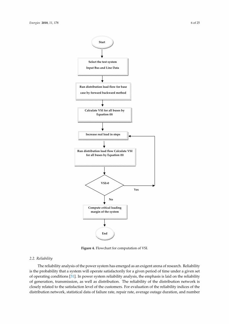
Figure 4. Flowchart for computation of VSI.

2.2. Reliability

The reliability analysis of the power system has emerged as an exigent arena of research. Reliability is the probability that a system will operate satisfactorily for a given period of time under a given set of operating conditions [31]. In power system reliability analysis, the emphasis is laid on the reliability of generation, transmission, as well as distribution. The reliability of the distribution network is closely related to the satisfaction level of the customers. For evaluation of the reliability indices of the distribution network, statistical data of failure rate, repair rate, average outage

Start

Select the test system

Input Bus and Line Data

Run distribution load flow for base

case by forward backward method

Compute critical loading margin of the system

Increase real load in steps

Run distribution load flow Calculate VSI for all buses by Equation (8)

Calculate VSI for all buses by Equation (8)

VSI>0

Yes

No

End

Figure 4. Flowchart for computation of VSI.

2.2. Reliability

The reliability analysis of the power system has emerged as an exigent arena of research. Reliabilityis the probability that a system will operate satisfactorily for a given period of time under a given setof operating conditions [31]. In power system reliability analysis, the emphasis is laid on the reliabilityof generation, transmission, as well as distribution. The reliability of the distribution network isclosely related to the satisfaction level of the customers. For evaluation of the reliability indices of thedistribution network, statistical data of failure rate, repair rate, average outage duration, and number

Energies 2018, 11, 178 7 of 25

of consumers of the buses or load points of the distribution network are required [31,32]. The detailedcategorization of the distribution network reliability indices is as shown in Figure 5. As mentioned inFigure 5 the reliability indices of distribution network are broadly categorized into customer orientedand energy oriented reliability indices. SAIFI, SAIDI, and CAIDI are the three major classifications ofcustomer oriented reliability indices. The energy oriented reliability indices can be again sub dividedinto ENS and AENS.

Energies 2018, 11, 178 7 of 25

Figure 5. Distribution Network Reliability Indices.

A comprehensive overview and the formulae of different customer and energy-oriented reliability indices are presented in Table 1. SAIFI and SAIDI are related to frequency and duration of interruption respectively. CAIDI gives a measure of customer dissatisfaction because of interruption. AENS can be regarded as the average load curtailment index because of interruption of service. The typical causes of the interruption are as follows:

• Outages resulting in interruption • Equipment failure disrupting the operation of the power system • Sudden increase in load demand resulting in load shedding • Scheduled maintenance requiring an interruption • Extreme weather damaging the infrastructure

Table 1. Overview of different customer and energy oriented reliability indices [31,32].

Index Definition Formula Physical Significance

SAIFI Number of times a system customer experiences interruption during a particular time period

j

jj

NNλ

SAIFI illustrates the condition of the system in terms of interruption

SAIDI Average interruption duration per customer served

j

jj

NNU

SAIDI illustrates the condition of the system in terms of duration of interruption

CAIDI Average interruption duration time for those customers interrupted during a year

jj

jj

NNU

λ CAIDI gives the average outage duration

that any given customer would experience.

ENS ENS gives the total energy not supplied by the system. jjUL ENS is an indicator of energy deficiency of

the system

AENS AENS is regarded as the average system load curtailment index

j

jj

NUL

AENS is the index giving an idea of how much energy is not served during a particular time period.

For further elaboration the flowchart for computation of the reliability indices is presented in Figure 6.

Distribution Network

Reliability Indices

Customer Oriented Reliability

Indices

Energy Oriented Reliability

Indices

SAIFI SAIDI CAIDI ENS AENS

Figure 5. Distribution Network Reliability Indices.

A comprehensive overview and the formulae of different customer and energy-oriented reliabilityindices are presented in Table 1. SAIFI and SAIDI are related to frequency and duration of interruptionrespectively. CAIDI gives a measure of customer dissatisfaction because of interruption. AENS can beregarded as the average load curtailment index because of interruption of service. The typical causesof the interruption are as follows:

• Outages resulting in interruption• Equipment failure disrupting the operation of the power system• Sudden increase in load demand resulting in load shedding• Scheduled maintenance requiring an interruption• Extreme weather damaging the infrastructure

Table 1. Overview of different customer and energy oriented reliability indices [31,32].

Index Definition Formula Physical Significance

SAIFINumber of times a system customerexperiences interruption during aparticular time period

∑ λj Nj

∑ Nj

SAIFI illustrates the condition of the systemin terms of interruption

SAIDI Average interruption duration percustomer served

∑ Uj Nj

∑ Nj

SAIDI illustrates the condition of thesystem in terms of duration of interruption

CAIDIAverage interruption duration timefor those customers interruptedduring a year

∑ Uj Nj

∑ λj Nj

CAIDI gives the average outage durationthat any given customer would experience.

ENS ENS gives the total energy notsupplied by the system. ∑ LjUj

ENS is an indicator of energy deficiency ofthe system

AENS AENS is regarded as the averagesystem load curtailment index

∑ LjUj

∑ Nj

AENS is the index giving an idea of howmuch energy is not served during aparticular time period.

For further elaboration the flowchart for computation of the reliability indices is presented inFigure 6.

Energies 2018, 11, 178 8 of 25

Energies 2018, 11, 178 8 of 25

Figure 6. Flowchart for computation of reliability indices.

2.3. Power Losses

Power losses of a distribution network refer to typical I2R losses of the line [29]. For the two bus system represented in Figure 3 the mathematical expression for computing the line losses is as given in Equation (9):

rIPj2= (9)

and the total power losses of the system are given as in Equation (10):

=

=n

jjt PP

1 (10)

Start

Select the test system

Set j=1

j=j+1

= jSAIFISAIFI = jSAIDISAIDI

= jCAIDICAIDI = jAENSAENS

Compute

j

jjj N

NSAIFI

λ=

j

jjj N

NUSAIDI =

jj

jjj N

NUCAIDI

λ=

j

jjj N

NLAENS =

j=End bus

Yes

No

End

Figure 6. Flowchart for computation of reliability indices.

2.3. Power Losses

Power losses of a distribution network refer to typical I2R losses of the line [29]. For the two bussystem represented in Figure 3 the mathematical expression for computing the line losses is as given inEquation (9):

Pj = I2r (9)

and the total power losses of the system are given as in Equation (10):

Pt =n

∑j=1

Pj (10)

From Equation (9) and Equation (10) it is clear that increase in load demand of even a single buswill contribute to net increase in power losses of the distribution network.

Energies 2018, 11, 178 9 of 25

2.4. Economic Losses

Voltage deviation beyond a certain limit and AENS are critical for the system and impose penaltyon the utility thereby causing economic loss. For the IEEE 33 bus system the voltage beyond whichpenalty is imposed is 0.9 per unit. The penalty imposed is given as in Equation (11):

Penalty = Voltage Deviation2 × 1, 000, 000 if V < 0.9 (11)

All the reliability indices explained in Section 2.2 can be utilized to decide a criterion for penaltyimposed on utility. In this work penalty imposed for unreliability is expressed in terms of AENS.Numerically it is 0.18 $/kWh energy not served.

2.5. Computational Methodology for Analyzing the Impact of EV Charging Station Load on Distribution Network

It is anticipated that the coming years will witness a rapid and significant EV charging loadintegration to the power distribution network. In this context, the impact of EV charging station loadon economic loss and different operating parameters of the distribution network must be analysed fordifferent scenarios of placement of EV charging stations.

The methodology adopted in the work for analysing the impact of EV charging station load onthe distribution network is illustrated in Figure 7.

Energies 2018, 11, 178 9 of 25

From Equation (9) and Equation (10) it is clear that increase in load demand of even a single bus will contribute to net increase in power losses of the distribution network.

2.4. Economic Losses

Voltage deviation beyond a certain limit and AENS are critical for the system and impose penalty on the utility thereby causing economic loss. For the IEEE 33 bus system the voltage beyond which penalty is imposed is 0.9 per unit. The penalty imposed is given as in Equation (11):

× <2Penalty=Voltage Deviation 1,000,000 if 0.9V (11)

All the reliability indices explained in Section 2.2 can be utilized to decide a criterion for penalty imposed on utility. In this work penalty imposed for unreliability is expressed in terms of AENS. Numerically it is 0.18 $/kWh energy not served.

2.5. Computational Methodology for Analyzing the Impact of EV Charging Station Load on Distribution Network

It is anticipated that the coming years will witness a rapid and significant EV charging load integration to the power distribution network. In this context, the impact of EV charging station load on economic loss and different operating parameters of the distribution network must be analysed for different scenarios of placement of EV charging stations.

The methodology adopted in the work for analysing the impact of EV charging station load on the distribution network is illustrated in Figure 7.

Figure 7. Flowchart of computational methodology for analyzing impact of EV charging station load on Distribution Network.

Start

Select the test system and input line data, bus data and outage data

Compute VSF and designate strong and weak buses of the network

Select test cases

Analyze the impact of EV charging stations on distribution network for all the test cases

Print results

Compute VSI for all the test cases

Compute SAIFI, SAIDI, CAIDI, and AENS for all

the test cases

Compute power losses and economic loss for all

the test cases

Figure 7. Flowchart of computational methodology for analyzing impact of EV charging station loadon Distribution Network.

3. VRP Index

In power system studies there is a dearth of indices giving information about the three mainoperating parameters like voltage stability, reliability, and power losses together. Hence, a new indexnamed Voltage Stability, Reliability and Power loss (VRP) index is formulated in this work. This index

Energies 2018, 11, 178 10 of 25

gives information about three prime operating parameters of the distribution network after the networkis subjected to any sort of disturbance. This index can be applied for:

• Optimal placement of charging stations.• Distribution network planning in presence of distributed generation.• Microgrid planning.• Reconfiguration of distribution networks.

The mathematical formulation of the VRP index is exemplified in this subsection by Equation (12)to Equation (16):

VRP = w1 A + w2B + w3C (12)

A =1a

(13)

a =VSIl

VSIbase(14)

B = w21SAIFIl

SAIFIbase+ w22

SAIDIlSAIDIbase

+ w23CAIDIl

CAIDIbase(15)

C =Pl

lossPloss base

(16)

Charging Station Placement Based on VRP Index

As a motivating example for the usage of the VRP index, we present briefly a novel methodologyfor the placement of the charging stations in the distribution network based on this index. The mainobjective of charging station placement problem is optimal allocation of EV charging stations in thedistribution network in such a way that the operating parameters of the distribution network are leastaffected. Thus, VRP index is selected as the objective function for charging station placement problembecause of its capability of taking into account voltage stability, reliability and power losses under asingle umbrella.

The decision variables, objective functions, and constraints for the optimal placement of chargingstations in the distribution network based on VRP index are presented in this sub-section.

The decision variables are:

• Buses of the distribution network in which charging stations will be placed, d• Number of fast charging stations placed at the buses, f• Number of slow charging stations placed at the buses, s

The optimization is aimed at minimization of VRP index. Mathematically:

min(VRP) where VRP = f (d, f , s) (17)

Subject to the following constraints:

0 ≤ ni ≤ n f astCS0 ≤ ni ≤ nslowCSSmin ≤ Si ≤ Smax

L ≤ Lmax

(18)

In addition to the aforementioned constraints, the power flow balance equation must be takenas an equality constraint. A flowchart illustrating the optimal placement of charging stations basedon the VRP index is shown in Figure 8, where as shown, the EV charger load is first modelled andthe test cases are simulated. Then, the impact of the EV charging station load on voltage stability,reliability, and power loss is evaluated for all the test cases A comparative analysis of the impact of the

Energies 2018, 11, 178 11 of 25

EV charging station load on the aforementioned parameters is made so that appropriate weights canbe assigned to all the terms of the VRP index. The weights assignment of the individual terms of theVRP index is based on the change in the operating parameters after the introduction of the EV chargingstation load. The most severely affected parameter is assigned the highest weight. After formulation ofthe VRP index the charging station placement problem is formulated. Lastly, optimization is performedand charging stations are allocated optimally in the distribution network.

Energies 2018, 11, 178 11 of 25

In addition to the aforementioned constraints, the power flow balance equation must be taken as an equality constraint. A flowchart illustrating the optimal placement of charging stations based on the VRP index is shown in Figure 8, where as shown, the EV charger load is first modelled and the test cases are simulated. Then, the impact of the EV charging station load on voltage stability, reliability, and power loss is evaluated for all the test cases A comparative analysis of the impact of the EV charging station load on the aforementioned parameters is made so that appropriate weights can be assigned to all the terms of the VRP index. The weights assignment of the individual terms of the VRP index is based on the change in the operating parameters after the introduction of the EV charging station load. The most severely affected parameter is assigned the highest weight. After formulation of the VRP index the charging station placement problem is formulated. Lastly, optimization is performed and charging stations are allocated optimally in the distribution network.

Figure 8. Flowchart for charging station placement based on VRP index.

4. Results

Massive penetration of EVs increases the load demand thereby degrading the operating parameters of the distribution network. The impact of the EV charging station load on voltage stability, power loss, reliability, and economic losses of the distribution network were analysed for

Start

Select the test system

Model EV charger load and select test cases for analysis

Assign proper weights to each parameter of

VRP index

Analyze the impact of EV charging station on

• Voltage Stability • Reliability • Power loss

Perform optimization

Formulate the charging station placement problem

Print results

Perform comparative analysis of the impact of EV charging station on Voltage

stability, Reliability, Power loss

Figure 8. Flowchart for charging station placement based on VRP index.

4. Results

Massive penetration of EVs increases the load demand thereby degrading the operatingparameters of the distribution network. The impact of the EV charging station load on voltagestability, power loss, reliability, and economic losses of the distribution network were analysed fordifferent scenarios and a charging station placement scheme based on the VRP index is presented inthis work. The results of the aforementioned analyses are presented in this section.

Energies 2018, 11, 178 12 of 25

4.1. Description of the Test System and Different Scenarios Considered for Analysis

The entire analysis was performed on IEEE 33 bus test system. This network is a radial network asillustrated in Figure 9. It is a distribution network with 33 bus and 32 branches. The line data,branch data, as well as reliability data of this test network were taken from references [33,34](See Tables A1–A3).

Energies 2018, 11, 178 12 of 25

different scenarios and a charging station placement scheme based on the VRP index is presented in this work. The results of the aforementioned analyses are presented in this section.

4.1. Description of the Test System and Different Scenarios Considered for Analysis

The entire analysis was performed on IEEE 33 bus test system. This network is a radial network as illustrated in Figure 9. It is a distribution network with 33 bus and 32 branches. The line data, branch data, as well as reliability data of this test network were taken from references [33,34] (See Tables A1–A3).

Figure 9. IEEE 33 bus Test Network.

Based on the methodology of computing VSF of the buses described in Equation (1) of Section 2.1.1 the strong and weak buses of the system were determined. Figure 10 illustrates the PV curve of the IEEE 33 bus system for different loading factors. From the figure, it is clear that as the loading of the system increases the deviation of the bus voltage from base values becomes more and more prominent. Table 2 reports the VSF of all the buses for different loading factor. The VSF of bus 14 for loading factor 2, 3, and 4 were 0.1163, 0.2707, and 0.5533, respectively. The values of VSF of bus 14 were highest in comparison to the other buses. Thus, bus 14 was regarded as the weakest bus of the system. Similarly, the VSF of bus 2 was least for all the loading factors making it the strongest bus of the system. The VSF values also signify that bus 19 and bus 15 were the second strongest and second weakest bus respectively.

Figure 10. PV curve with load increased in steps in all the buses.

Figure 9. IEEE 33 bus Test Network.

Based on the methodology of computing VSF of the buses described in Equation (1) of Section 2.1.1the strong and weak buses of the system were determined. Figure 10 illustrates the PV curve of theIEEE 33 bus system for different loading factors. From the figure, it is clear that as the loading of thesystem increases the deviation of the bus voltage from base values becomes more and more prominent.Table 2 reports the VSF of all the buses for different loading factor. The VSF of bus 14 for loadingfactor 2, 3, and 4 were 0.1163, 0.2707, and 0.5533, respectively. The values of VSF of bus 14 werehighest in comparison to the other buses. Thus, bus 14 was regarded as the weakest bus of the system.Similarly, the VSF of bus 2 was least for all the loading factors making it the strongest bus of the system.The VSF values also signify that bus 19 and bus 15 were the second strongest and second weakestbus respectively.

Energies 2018, 11, 178 12 of 25

different scenarios and a charging station placement scheme based on the VRP index is presented in this work. The results of the aforementioned analyses are presented in this section.

4.1. Description of the Test System and Different Scenarios Considered for Analysis

The entire analysis was performed on IEEE 33 bus test system. This network is a radial network as illustrated in Figure 9. It is a distribution network with 33 bus and 32 branches. The line data, branch data, as well as reliability data of this test network were taken from references [33,34] (See Tables A1–A3).

Figure 9. IEEE 33 bus Test Network.

Based on the methodology of computing VSF of the buses described in Equation (1) of Section 2.1.1 the strong and weak buses of the system were determined. Figure 10 illustrates the PV curve of the IEEE 33 bus system for different loading factors. From the figure, it is clear that as the loading of the system increases the deviation of the bus voltage from base values becomes more and more prominent. Table 2 reports the VSF of all the buses for different loading factor. The VSF of bus 14 for loading factor 2, 3, and 4 were 0.1163, 0.2707, and 0.5533, respectively. The values of VSF of bus 14 were highest in comparison to the other buses. Thus, bus 14 was regarded as the weakest bus of the system. Similarly, the VSF of bus 2 was least for all the loading factors making it the strongest bus of the system. The VSF values also signify that bus 19 and bus 15 were the second strongest and second weakest bus respectively.

Figure 10. PV curve with load increased in steps in all the buses. Figure 10. PV curve with load increased in steps in all the buses.

Energies 2018, 11, 178 13 of 25

Table 2. VSF at different loading factor.

Bus No. VSF at Loading Factor 2 VSF at Loading Factor 3 VSF at Loading Factor 4

2 0.0034 0.0074 0.01293 0.0196 0.0431 0.07644 0.0284 0.0631 0.11345 0.0372 0.0831 0.15096 0.0593 0.1335 0.24617 0.0636 0.1436 0.26628 0.0803 0.1826 0.34529 0.0882 0.2015 0.385710 0.0956 0.2192 0.425011 0.0967 0.2218 0.431112 0.0986 0.2265 0.442013 0.1064 0.2458 0.487714 0.1163 0.2707 0.553315 0.1156 0.2687 0.547716 0.1129 0.2621 0.529717 0.1112 0.2576 0.517918 0.1093 0.2530 0.506019 0.0039 0.0085 0.014620 0.0076 0.0158 0.025721 0.0083 0.0173 0.027922 0.0089 0.0186 0.029923 0.0234 0.0510 0.089024 0.0305 0.0659 0.112625 0.0341 0.0733 0.124526 0.0617 0.1389 0.256327 0.0647 0.1460 0.270128 0.0786 0.1780 0.332429 0.0886 0.2015 0.379630 0.0930 0.2118 0.401131 0.0981 0.2241 0.427332 0.0993 0.2268 0.433233 0.0996 0.2277 0.4351

Figure 11 gives the comparative analysis of voltage of all the buses for the base case and criticalloading. From the figure, the deviation of voltage of all the buses is quite prominent.

Energies 2018, 11, 178 13 of 25

Table 2. VSF at different loading factor.

Bus No. VSF at Loading Factor 2 VSF at Loading Factor 3 VSF at Loading Factor 4 2 0.0034 0.0074 0.0129 3 0.0196 0.0431 0.0764 4 0.0284 0.0631 0.1134 5 0.0372 0.0831 0.1509 6 0.0593 0.1335 0.2461 7 0.0636 0.1436 0.2662 8 0.0803 0.1826 0.3452 9 0.0882 0.2015 0.3857

10 0.0956 0.2192 0.4250 11 0.0967 0.2218 0.4311 12 0.0986 0.2265 0.4420 13 0.1064 0.2458 0.4877 14 0.1163 0.2707 0.5533 15 0.1156 0.2687 0.5477 16 0.1129 0.2621 0.5297 17 0.1112 0.2576 0.5179 18 0.1093 0.2530 0.5060 19 0.0039 0.0085 0.0146 20 0.0076 0.0158 0.0257 21 0.0083 0.0173 0.0279 22 0.0089 0.0186 0.0299 23 0.0234 0.0510 0.0890 24 0.0305 0.0659 0.1126 25 0.0341 0.0733 0.1245 26 0.0617 0.1389 0.2563 27 0.0647 0.1460 0.2701 28 0.0786 0.1780 0.3324 29 0.0886 0.2015 0.3796 30 0.0930 0.2118 0.4011 31 0.0981 0.2241 0.4273 32 0.0993 0.2268 0.4332 33 0.0996 0.2277 0.4351

Figure 11 gives the comparative analysis of voltage of all the buses for the base case and critical loading. From the figure, the deviation of voltage of all the buses is quite prominent.

Figure 11. Comparison between voltage of base case and critical loading case for all buses in per unit.

The EV charger load was modelled as in [28] and based on the data that a fast EV charger consumes 50 kW power [35] (See Table A4) the entire analysis was performed for all the cases illustrated in Table 3.

Figure 11. Comparison between voltage of base case and critical loading case for all buses in per unit.

The EV charger load was modelled as in [28] and based on the data that a fast EV charger consumes50 kW power [35] (See Table A4) the entire analysis was performed for all the cases illustrated inTable 3.

Energies 2018, 11, 178 14 of 25

Table 3. Different cases considered for analyzing the impact of placement of charging station.

Case Description Increase in Load (kW)

2 Fast Charging station is placed at bus 2 15003 Fast charging station is placed at bus 2 30004 Fast Charging station is placed at bus 2 75005 Fast Charging station is placed at bus 2 and bus 19 3000 (1500 each)6 Fast Charging station is placed at bus 14 15007 Fast Charging station is placed at bus 14 and bus 15 3000 (1500 each)

Case 1 was considered as the base case without charging stations in the entire analysis. In case 2 afast charging station was placed at bus 2 representing the strongest bus of the system with 30 servingpoints. Assuming that each charger consumes 50 kW the charging station possessed the capability ofcharging 30 EVs simultaneously. In case 3 two charging stations were placed at bus 2 and in case 4 fivefast charging stations were placed at bus 2. In case 5 a fast charging station was placed at bus 2 and 19representing the strongest and second strongest bus respectively. In case 6 a single fast charging stationwas placed at bus 14 representing the weakest bus of the system. In case 7 a fast charging station wasplaced at bus 14 and 15 representing the weakest and second weakest bus respectively.

4.2. Impact of EV Charging Station Load on Distribution Network

The impact of EV charging station load on voltage stability, reliability, power losses, and economiclosses of the distribution network was analysed for all the cases as mentioned in Table 3 and the resultsof this analyses are reported in this sub section.

4.2.1. Impact of EV Charging Station Load on Voltage Stability

The impact of EV charging load on voltage stability of IEEE 33 bus test network is reported in thissub section. The value of VSI is calculated for all the buses by utilizing the methodology elaborated inSection 2.1.2.

Table 4 reports the VSI for the base case and different cases of the placement of the EV chargingstation. It is observed that for case 7 where charging station was placed at the weakest bus the VSI ofbus 14 was as low as 0.2073. Thus, placement of charging station at the weakest bus caused severedegradation of the voltage stability.

Table 4. Impact of EV charging station load on VSI.

Bus No. VSI forBase Case

VSI forCase 2

VSI forCase 3

VSI forCase 4

VSI forCase 5

VSI forCase 6

VSI forCase 7

2 0.9998 0.9981 0.9981 0.9908 0.9981 0.9998 0.99973 0.9868 0.9834 0.9834 0.9696 0.9799 0.9815 0.97434 0.9327 0.9294 0.9294 0.9161 0.9261 0.9054 0.87095 0.9051 0.9018 0.9018 0.8887 0.8985 0.8622 0.80906 0.8766 0.8734 0.8734 0.8604 0.8701 0.8171 0.74387 0.8126 0.8095 0.8095 0.7971 0.8064 0.7248 0.62098 0.7961 0.7930 0.7930 0.7807 0.7899 0.6984 0.57889 0.7558 0.7528 0.7528 0.7408 0.7498 0.6052 0.4403

10 0.7355 0.7326 0.7326 0.7208 0.7296 0.5555 0.368711 0.7180 0.7151 0.7151 0.7034 0.7121 0.5114 0.309212 0.7151 0.7122 0.7122 0.7005 0.7093 0.5034 0.298413 0.7092 0.7063 0.7063 0.6947 0.7034 0.4871 0.274514 0.6905 0.6877 0.6877 0.6762 0.6848 0.4290 0.207315 0.6845 0.6816 0.6816 0.6702 0.6788 0.4180 0.186016 0.6800 0.6772 0.6772 0.6658 0.6744 0.4146 0.179217 0.6753 0.6725 0.6725 0.6612 0.6697 0.4109 0.176818 0.6695 0.6667 0.6667 0.6554 0.6639 0.4064 0.173919 0.9879 0.9846 0.9846 0.9708 0.9780 0.9834 0.977720 0.9837 0.9804 0.9804 0.9667 0.9709 0.9792 0.973521 0.9713 0.9680 0.9680 0.9544 0.9586 0.9669 0.961122 0.9680 0.9647 0.9647 0.9511 0.9553 0.9636 0.9579

Energies 2018, 11, 178 15 of 25

Table 4. Cont.

Bus No. VSI forBase Case

VSI forCase 2

VSI forCase 3

VSI forCase 4

VSI forCase 5

VSI forCase 6

VSI forCase 7

23 0.9329 0.9296 0.9296 0.9163 0.9262 0.9059 0.872024 0.9138 0.9105 0.9105 0.8973 0.9072 0.8871 0.853525 0.8892 0.8859 0.8859 0.8729 0.8827 0.8628 0.829726 0.8136 0.8105 0.8105 0.7980 0.8073 0.7258 0.622027 0.8069 0.8038 0.8038 0.7914 0.8007 0.7195 0.616228 0.7972 0.7941 0.7941 0.7818 0.7910 0.7103 0.607729 0.7589 0.7559 0.7559 0.7439 0.7529 0.6743 0.574430 0.7316 0.7286 0.7286 0.7168 0.7257 0.6485 0.550631 0.7208 0.7179 0.7179 0.7062 0.7150 0.6384 0.541332 0.7091 0.7062 0.7062 0.6946 0.7033 0.6274 0.531233 0.7069 0.7040 0.7040 0.6924 0.7011 0.6253 0.5293

Table 5 lists the voltage of all the buses for the base case as well as after placing charging stations forall the cases mentioned in Table 3. The voltage of bus 14 for case 2 was 0.9082 pu. Thus, the magnitudeof the voltage of bus 14 for case 2 was less than the base case voltage, but still within the acceptablerange. However, for case 4 when five charging stations were placed at bus 2 the voltages of bus 17 andbus 18 dropped to 0.8984 pu and 0.8978 pu respectively. These values were not within the tolerancelimit. In case 5 where a single charging station of 1500 kW was placed at bus 2 and bus 19 respectivelyit is observed that voltage drops of all the buses were less than that of case 3 where a single chargingstation of 3000 kW was placed at bus 2. Thus, distributing the charging stations between a number ofbuses is advantageous than concentrating the charging stations at a single bus. In case 6 where thecharging station was placed at bus 14 representing a weak bus the voltage dropped to 0.7351 whichcannot be tolerated. Similarly, for case 7 where two charging stations are placed at the two weak busesthe voltage drop was prominent.

Table 5. Impact of EV charging station load on voltage profile.

Bus No. Voltage forBase Case

Voltagefor Case 2

Voltagefor Case 3

Voltagefor Case 4

Voltagefor Case 5

Voltagefor Case 6

Voltagefor Case 7

2 0.9970 0.9959 0.9947 0.9913 0.9948 0.9954 0.99313 0.9829 0.9818 0.9806 0.9771 0.9807 0.9724 0.95804 0.9754 0.9743 0.9731 0.9696 0.9732 0.9584 0.93505 0.9680 0.9669 0.9657 0.9621 0.9658 0.9442 0.91146 0.9496 0.9484 0.9472 0.9436 0.9473 0.9084 0.85287 0.9461 0.9449 0.9437 0.9401 0.9438 0.8969 0.83228 0.9325 0.9313 0.9300 0.9264 0.9301 0.8501 0.74079 0.9262 0.9249 0.9237 0.9200 0.9238 0.8239 0.686710 0.9203 0.9191 0.9178 0.9141 0.9179 0.7979 0.631911 0.9195 0.9182 0.9170 0.9132 0.9171 0.7938 0.622812 0.9179 0.9167 0.9155 0.9117 0.9155 0.7863 0.605713 0.9118 0.9105 0.9093 0.9055 0.9094 0.7508 0.526414 0.9095 0.9082 0.9070 0.9032 0.9071 0.7351 0.491015 0.9081 0.9068 0.9056 0.9018 0.9056 0.7333 0.475216 0.9067 0.9054 0.9042 0.9004 0.9042 0.7316 0.472617 0.9047 0.9034 0.9022 0.8984 0.9022 0.7291 0.468818 0.9041 0.9028 0.9016 0.8978 0.9016 0.7284 0.467719 0.9965 0.9954 0.9942 0.9908 0.9921 0.9948 0.992620 0.9929 0.9918 0.9906 0.9872 0.9885 0.9912 0.989021 0.9922 0.9911 0.9899 0.9865 0.9878 0.9905 0.988322 0.9916 0.9904 0.9893 0.9858 0.9871 0.9899 0.987623 0.9793 0.9782 0.9770 0.9735 0.9771 0.9688 0.954324 0.9727 0.9715 0.9703 0.9668 0.9704 0.9620 0.947525 0.9693 0.9682 0.9670 0.9635 0.9671 0.9587 0.944126 0.9477 0.9465 0.9453 0.9417 0.9454 0.9064 0.850627 0.9451 0.9439 0.9427 0.9391 0.9428 0.9037 0.847828 0.9337 0.9325 0.9313 0.9276 0.9314 0.8917 0.835029 0.9255 0.9243 0.9231 0.9193 0.9231 0.8831 0.825830 0.9220 0.9207 0.9195 0.9158 0.9196 0.8794 0.821831 0.9178 0.9166 0.9153 0.9116 0.9154 0.8750 0.817232 0.9169 0.9156 0.9144 0.9107 0.9145 0.8741 0.816133 0.9166 0.9154 0.9141 0.9104 0.9142 0.8738 0.8158

Energies 2018, 11, 178 16 of 25

4.2.2. Impact of EV Charging Station Load on Reliability

The impact of EV charging station load on the reliability of the distribution network was analysedfor all the cases mentioned in Table 3. The results of this analysis are reported in this sub-section.The failure rate, repair rate and outage duration of the system for increased load demand werecomputed based on unitary method [33].

Table 6 reports the impact of the placement of the EV charging stations on different reliabilityindices. The value of SAIFI for case 2 was 0.1195 interruption/customer yr. This value was more thanthe base case SAIFI but less than the critical or dead zone value of SAIFI. Similar trend is observedfor SAIDI, CAIDI, as well as AENS. It is observed that for case 6 and case 7 the reliability indicesdegraded to a value that cannot be tolerated. Thus, for an increased load demand due to EV chargingload the interruption, duration of interruption per customer increased. These were the chief causes ofcustomer dissatisfaction.

Table 6. Impact of EV charging station load on different reliability indices.

Case SAIFI (Interruption/Year) SAIDI (h/Year) CAIDI (h/Interruption) AENS (kWh/Year)

Base case 0.0982 0.5048 5.1385 1.93692 0.1195 0.6321 5.2915 10.26123 0.1407 0.7594 5.3984 33.274 0.2043 1.1413 5.5858 314.50495 0.1361 0.7155 5.2558 16.35476 0.1235 0.7578 6.1341 15.15787 0.1366 0.8448 6.1850 23.9717

For further analysis, Table 7 reports the equivalent events like increase in the number of customersresponsible for degrading the reliability indices. Table 7 reports that the establishment of charginginfrastructure of 30, 60, and 150 EVs is equivalent to increasing the number of customer of thedistribution network by 106, 154, and 254 respectively in terms of the degradation of SAIFI.

Table 7. Equivalent events producing the SAIFI similar to addition of charging station.

Case Number of EVs ThatCan Be Charged SAIFI Increase in Load Producing

Same SAIFI (kW)Increase in Number of Consumers

Producing Same SAIFI

2 30 0.1195 407.69 1063 60 0.1407 590.095 1544 150 0.2043 976.45 254

4.2.3. Impact of EV Charging Station Load on Power Loss

The impact of the EV charging station load on the power loss of the distribution network wereanalysed for all the cases as mentioned in Table 3 and the results of this analysis are reported in thissubsection. The power loss of the distribution network was computed by Equation (10).

Table 8 reports the magnitude of power loss of the network for different cases of placement ofcharging station. The power loss of the distribution network after the placement of charging stationswas high as compared to without the charging stations. The power loss of case 5 is less than that ofcase3 signifying the advantage of distributing the charging station load between two buses. For case 6and 7 where charging stations were placed at weak buses, the power losses were 0.0090 and 0.0247respectively. Thus, these values were quite high in comparison to the base case.

4.2.4. Impact of EV Charging Station Load on Economic Loss

A detailed analysis of the economic losses incurred because of degradation of voltage profileand reliability indices are reported in this subsection. Table 9 reports the economic losses incurredby the utility due degradation of voltage profile and reliability after placement of charging stations.

Energies 2018, 11, 178 17 of 25

For case 2, case 3 and case 4 where charging stations were placed at the strongest bus of the networkthe penalty for voltage deviation was almost negligible. However, for case 4 the penalty for AENSwas 56.610 $. On the other hand, when charging station was placed at bus 14 the penalty for voltagedeviation was as high as 70,289 $. Despite the fact that improper placement of charging station resultsin economic losses the EVs must be welcomed as the net benefit earned by implementing V2G schemecannot be neglected.

Table 8. Impact of EV charging station load on power loss.

Case Power Loss (pu)

Base case 0.00212 0.00223 0.00244 0.0035 0.00236 0.00907 0.0247

Table 9. Impact of EV charging station load on economic loss.

Case Penalty for Voltage Deviation ($) Penalty for Energy Not Supplied ($)

2 0 1.843 0 5.98864 0.4892 56.6105 0 2.94386 70,289 2.7287 1,397,700 4.3149

4.2.5. Comparative Analysis of EV Charging Station Load on Voltage Stability, Power Loss,and Reliability

A comparative analysis of the impact of EV charging station load on different operationalparameters of the system like voltage stability, power loss, and reliability was performed and theresults are in this sub-section.

Table 10 gives a comparative analysis of the effect of EV charging station load on different indicesof the distribution network. From this table it is clear that the reliability indices were more affectedthan power loss and voltage stability for case 2, case 3 and case 4 where charging station was placed atstrong buses. However, for case 7 where charging stations were placed at bus 14 and 15 power losswas most severely affected. As illustrated in Figure 12 for case 4 the power loss is affected less thanreliability indices. On the other hand, as illustrated in Figure 13 the % change in power loss for case 7is 85%.

Table 10. Comparative Analysis of different parameters after placement of charging stations.

CaseChange in

VSI Power Loss SAIFI SAIDI CAIDI

2 0.00173 0476 0.2169 0.2521 0.02973 0.00362 0.1428 0.4327 0.5043 0.05054 0.00912 0.42857 1.08044 1.26 0.087625 0.00347 0.0952 0.3859 0.417 0.02286 0.1950 2.1904 0.417 0.5011 0.19377 0.3299 8.9523 0.0228 0.67022 0.2036

Energies 2018, 11, 178 18 of 25Energies 2018, 11, 178 18 of 25

0% 15%

38%44%

3%

% change

VSI of weakest bus Power loss SAIFI SAIDI CAIDI

Figure 12. Comparative analysis of placement of charging station on VSI, power loss and reliability indices for Case 4.

Figure 13. Comparative analysis of placement of charging station on VSI, power loss and reliability indices for Case 7.

4.3. Optimal Placement of Charging Stations Based on VRP Index

As a motivating example for the usage of VRP index, we present briefly a novel methodology for the placement of the charging stations in the distribution network based on the VRP index. Genetic algorithm (GA) was used for solving the optimization problem. The results of the optimal placement of the charging stations are reported in this subsection. Table 11 reports the values of the different input parameters required for performing optimization. Table 12 reports the optimal locations of the charging stations in the IEEE 33 bus distribution network computed based on VRP index. The optimal locations were bus number 19, 20, and 2. The number of fast charging stations placed at bus number 19, 20, and 2 were 2, 1, and 2 respectively. The number of slow charging stations placed at bus number 19, 20, and 2 were 3, 2, and 1 respectively.

Table 11. Input Parameters.

Parameter Value1w 0.1

2w 0.7

3w 0.2

21w 0.2

22w 0.4

23w 0.1 nfastCS 2 nslowCS 3

Figure 12. Comparative analysis of placement of charging station on VSI, power loss and reliabilityindices for Case 4.

Energies 2018, 11, 178 18 of 25

0% 15%

38%44%

3%

% change

VSI of weakest bus Power loss SAIFI SAIDI CAIDI

Figure 12. Comparative analysis of placement of charging station on VSI, power loss and reliability indices for Case 4.

Figure 13. Comparative analysis of placement of charging station on VSI, power loss and reliability indices for Case 7.

4.3. Optimal Placement of Charging Stations Based on VRP Index

As a motivating example for the usage of VRP index, we present briefly a novel methodology for the placement of the charging stations in the distribution network based on the VRP index. Genetic algorithm (GA) was used for solving the optimization problem. The results of the optimal placement of the charging stations are reported in this subsection. Table 11 reports the values of the different input parameters required for performing optimization. Table 12 reports the optimal locations of the charging stations in the IEEE 33 bus distribution network computed based on VRP index. The optimal locations were bus number 19, 20, and 2. The number of fast charging stations placed at bus number 19, 20, and 2 were 2, 1, and 2 respectively. The number of slow charging stations placed at bus number 19, 20, and 2 were 3, 2, and 1 respectively.

Table 11. Input Parameters.

Parameter Value1w 0.1

2w 0.7

3w 0.2

21w 0.2

22w 0.4

23w 0.1 nfastCS 2 nslowCS 3

Figure 13. Comparative analysis of placement of charging station on VSI, power loss and reliabilityindices for Case 7.

4.3. Optimal Placement of Charging Stations Based on VRP Index

As a motivating example for the usage of VRP index, we present briefly a novel methodology forthe placement of the charging stations in the distribution network based on the VRP index. Geneticalgorithm (GA) was used for solving the optimization problem. The results of the optimal placementof the charging stations are reported in this subsection. Table 11 reports the values of the differentinput parameters required for performing optimization. Table 12 reports the optimal locations of thecharging stations in the IEEE 33 bus distribution network computed based on VRP index. The optimallocations were bus number 19, 20, and 2. The number of fast charging stations placed at bus number 19,20, and 2 were 2, 1, and 2 respectively. The number of slow charging stations placed at bus number 19,20, and 2 were 3, 2, and 1 respectively.

Table 11. Input Parameters.

Parameter Value

w1 0.1w2 0.7w3 0.2w21 0.2w22 0.4w23 0.1

nfastCS 2nslowCS 3

Energies 2018, 11, 178 19 of 25

Table 12. Optimal Placement of Charging Stations based on VRP index.

Bus No. Number of Fast Charging Stations Number of Slow Charging Stations

19 2 320 1 22 2 1

5. Discussion

EVs reduce the local emissions and have a positive impact on the environment. However,the detrimental impact of the EV charging station loads on the electricity distribution network cannotbe neglected. The focus of this work was to present a detailed analysis of the impact of the EV chargingstation load on the different technical as well as economic parameters of the IEEE 33 bus system.The impact of the EV charging stations on the voltage stability, reliability, power loss, and economicloss were analysed profoundly in this work and the key findings of the work are summarized as follows:

(1) The IEEE 33 bus test system was robust enough to withstand the placement of four chargingstations at bus 2 representing the strongest bus of the system. It is observed that when fivecharging stations were placed at bus 2 the SAIDI increased by 44%. Thus, for increasing thenumber of charging stations beyond four up gradation of the network was required.

(2) The placement of the fast charging station at the weak bus of the network was detrimental to thesecurity of the system. On placement of even a single charging station at the weakest bus thevoltage of the weakest bus dropped to 0.7351 per unit. The reliability indices also deterioratedsignificantly on placement of fast charging stations at the weak buses. Moreover, it is observedthat on placement of a single charging station at bus 14 and 15 representing the weak buses of thenetwork the power losses increased by 85%. However, slow charging stations of 19.2 kW couldbe placed even at the weak buses.

(3) Distributing the charging stations between a number of buses was advantageous thanconcentrating the charging stations at a single bus in terms of voltage deviation, reliabilityas well as power loss. Also, in some cases, if the strong nodes of the distribution network andnodes of the road network with high traffic concentration merge then the routes leading to thatnode will be too congested. Therefore, another advantage of distributing the charging stationis making the charging facility accessible to a larger number of EVs plying in different routes.This in turn will reduce the traffic congestion of the specific routes leading to the bus in whichcharging stations are concentrated.

(4) A considerable economic loss was incurred by the utility for placement of charging stations at theweak buses. It is observed that on placement of even a single fast charging station at the weakestbus 1,397,700.5 $ of economic loss is incurred. However, despite the fact that improper placementof charging station results in economic losses the EVs must be welcomed as the net benefit earnedby implementing V2G scheme cannot be neglected. In V2G scheme the charging stations canearn revenue by selling the electricity back to the grid when the charging demand is low.

(5) The reliability indices were more affected than power loss and voltage stability for case 2, case 3and case 4 where the charging station was placed at strong buses. However, for case 7 wherecharging stations are placed at bus 14 and 15 power loss was most severely affected.

All the aforementioned findings must be taken into account while dealing with the problem ofoptimal placement of charging stations. From the results obtained it is obvious that voltage stability,power loss as well as reliability indices degraded with the addition of EV charging station loads. Thus,for optimal placement of charging stations in the distribution network all the three parameters mustbe considered. A novel index named VRP index taking into account the voltage stability, reliabilityand power loss was also formulated. The novelty of VRP index lies in the fact that has the capabilityof considering voltage stability, power loss, and reliability together under a common frame. Further,

Energies 2018, 11, 178 20 of 25

a strategy for the placement of the charging stations in the distribution network based on VRP indexwas presented in this work. The results of the optimal placement of the charging stations based onVRP index established the efficacy of the index. Future possible research directions in this area are:

(1) Mitigation of the negative impacts of EV charging station placement by reconfiguration ofthe network.

(2) Analysis of the positive impact of the Vehicle to Grid (V2G) scheme.(3) Real time planning of EV charging stations based on VRP index.

6. Conclusions

EVs are a favorable alternative to reduce the emissions of the transport sector. The growingpopularity of EVs has led to the establishment of charging stations; however the detrimental impact ofthe resulting EV charging station loads on the distribution network cannot be neglected. This workmeticulously analysed the impact of EV charging station loads on the voltage stability, reliabilityindices, power losses, and economic loss of the IEEE 33 bus test system. The results obtained showedthat the impact of placing fast charging stations at the weak buses affected the smooth operation ofthe power distribution network. A considerable amount of economic loss was also incurred if fastcharging stations were placed at the weak buses of the network. However, the system was strongenough to withstand the placement of charging stations at the strong buses. Further, the placementof the charging stations in the distribution network based on a new VRP index was proposed in thiswork. GA was used to solve the charger location problem with VRP index as the objective function.The results obtained indicate the efficacy of the VRP index in finding the most suitable locations forcharging stations in the IEEE 33 bus test network. Thus, this work will serve as a guide to the powersystem engineers and help in planning of distribution networks in presence of EV charging loads.

Acknowledgments: The authors would like to thank Henry Ford Foundation Finland for support.

Author Contributions: The work is performed by Sanchari Deb under the supervision of Karuna Kalita,Pinakeshwar Mahanta and Kari Tammi. Kari Tammi participated in drafting the research problem, outlining thesolution procedure, and checking the methodology and results. Karuna Kalita and Pinakeshwar Mahanta helpedin writing the article.

Conflicts of Interest: The authors declare no conflict of interest.

Nomenclature

EV Electric VehicleVRP Voltage Stability, Reliability, and Power loss IndexICE Internal Combustion EngineIPT Inductive Power TransferPHEV Plugged In Hybrid Electric VehiclePV curve Power and Voltage curveVSF Voltage Sensitivity FactorVSI Voltage Stability IndexSAIFI System Average Interruption Frequency IndexSAIDI System Average Interruption Duration IndexCAIDI Customer Average Interruption Duration IndexENS Energy Not ServedAENS Average Energy Not ServedVj < δj Voltage of bus jVj+1 < δj+1 Voltage of bus j + 1I Current flowing through the branch having resistance r and impedance xPj+1 Active power of the bus j + 1

Energies 2018, 11, 178 21 of 25

Qj+1 Reactive power of bus j + 1Z Impedance of branch jλj Failure rate of bus jNj Number of consumers connected at bus jUj Annual outage duration of bus jLj Load demand of bus jPj Power losses through jth branchPt Total power losses of the networkw1 Weight assigned to Aw2 Weight assigned to Bw3 Weight assigned to CVSIl VSI after increase in loadSAIFIl SAIFI after increase in loadSAIDIl SAIDI after increase in loadCAIDIl CAIDI after increase in loadVSIbase Base value of VSISAIFIbase Base value of SAIFISAIDIbase Base value of SAIDICAIDIbase Base value of CAIDIPl

loss Power losses after increase in loadPloss base Power losses for the base casew21 Sub weight assigned to SAIFIw22 Sub weight assigned to SAIDIw23 Sub weight assigned to CAIDIi Index of strong bus of the networkn Number of charging stations placed at bus infastCS Maximum number of fast charging stations that can be placed at each busnslowC Maximum number of slow charging stations that can be placed at each busSmin Lower bound of reactive powerSmax Upper bound of reactive powerLmax Loading margin of the network

Appendix

Table A1. Bus Data of IEEE 33 bus test system [34].

Bus No. Real Power (pu) Reactive Power (pu)

1 0 02 0.0010 0.00063 0.0009 0.00044 0.0012 0.00085 0.0006 0.00036 0.0006 0.00027 0.0020 0.00108 0.0020 0.00109 0.0006 0.0002

10 0.0006 0.000211 0.0004 0.000312 0.0006 0.000413 0.0006 0.000414 0.0012 0.000815 0.0006 0.000116 0.0006 0.000217 0.0006 0.000218 0.0009 0.0004

Energies 2018, 11, 178 22 of 25

Table A1. Cont. [34]

Bus No. Real Power (pu) Reactive Power (pu)

19 0.0009 0.000420 0.0009 0.000421 0.0009 0.000422 0.0009 0.000423 0.0009 0.000524 0.0042 0.002025 0.0042 0.002026 0.0006 0.000327 0.0006 0.000328 0.0006 0.000229 0.0012 0.000730 0.0020 0.006031 0.0015 0.000732 0.0021 0.001033 0.0006 0.0004

Table A2. Line Data of IEEE 33 bus test system [34].

Line No. Starting Bus End Bus R (pu) X (pu)

1 1 2 0.0575 0.02982 2 3 0.3076 0.15673 3 4 0.2284 0.11634 4 5 0.2378 0.12115 5 6 0.5110 0.44116 6 7 0.1168 0.38617 7 8 1.0678 0.77068 8 9 0.6426 0.46179 9 10 0.6489 0.461710 10 11 0.1227 0.040611 11 12 0.2336 0.077212 12 13 0.9159 0.720613 13 14 0.3379 0.444814 14 15 0.3687 0.328215 15 16 0.4656 0.340016 16 17 0.8042 1.073817 17 18 0.4567 0.358118 2 19 0.1023 0.097619 19 20 0.9385 0.845720 20 21 0.2555 0.298521 21 22 0.4423 0.584822 3 23 0.2815 0.192423 23 24 0.5603 0.442424 24 25 0.5590 0.437425 6 26 0.1267 0.064526 26 27 0.1773 0.090327 27 28 0.6607 0.582628 28 29 0.5018 0.437129 29 30 0.3166 0.161330 30 31 0.6080 0.600831 31 32 0.1937 0.225832 32 33 0.2128 0.3308

Energies 2018, 11, 178 23 of 25

Table A3. Outage Data of IEEE 33 bus test system [33].

Bus No. Failure Rate (Failure/Year) Outage Duration (h/Year) No. of Consumer Load (kW)

2 0.0500 0.3000 26 1003 0.0400 0.3000 23 904 0.0600 0.3000 31 1205 0.0300 0.2000 16 606 0.0300 0.2000 16 2007 0.0900 0.6000 52 2008 0.0300 0.6000 52 609 0.0300 0.2000 15 60

10 0.0200 0.2000 15 4511 0.0300 0.1000 12 6012 0.0300 0.2000 16 6013 0.0600 0.2000 16 12014 0.0300 0.3000 31 6015 0.0300 0.2000 16 6016 0.0300 0.2000 16 6017 0.0300 0.2000 16 6018 0.0400 0.2000 23 9019 0.0400 0.2000 23 9020 0.0400 0.2000 23 9021 0.0400 0.2000 23 9022 0.0400 0.2000 23 9023 0.0400 0.2000 23 9024 0.1900 1.1000 109 42025 0.1900 1.1000 109 42026 0.0300 0.2000 16 6027 0.0300 0.2000 16 6028 0.0300 0.2000 16 6029 0.5400 0.3000 31 12030 0.0900 0.5000 25 12031 0.0700 0.4000 39 15032 0.1000 0.6000 35 21033 0.0300 0.2000 16 60

Table A4. Charging station specifications for EV [35].

Type Load Consumed (kW)

Level 1 Up to 1.8Level 2 Up to 19.2

DC Fast charging (50–150)

References

1. Wang, Z.; Yang, L. Delinking indicators on regional industry development and carbon emissions:Beijing–Tianjin–Hebei economic band case. Ecol. Indic. 2015, 48, 41–48. [CrossRef]

2. Wang, Q.; Rongrong, L.; Rui, J. Decoupling and Decomposition Analysis of Carbon Emissions from Industry:A Case Study from China. Sustainability 2016, 10, 1059–1076. [CrossRef]

3. Blesl, M.; Das, A.; Fahl, U.; Remme, U. Role of energy efficiency standards in reducing CO2 emissions inGermany: An assessment with TIMES. Energy Policy 2007, 35, 772–785. [CrossRef]

4. Alam, M.M.; Mekhilef, S.; Seyedmahmoudian, M.; Horan, B. Dynamic Charging of Electric Vehicle withNegligible Power Transfer Fluctuation. Energies 2017, 10, 701. [CrossRef]

5. Foley, A.M.; Winning, I.J.; Gallachóir, B.P. State-of-the-art in electric vehicle charging infrastructure.In Proceedings of the Vehicle Power and Propulsion (VPPC), Lille, France, 1–3 September 2010; pp. 1–6.

Energies 2018, 11, 178 24 of 25

6. Shi, R.; Zhang, X.P.; Kong, D.C.; Wang, P.Y. Dynamic Impacts of Fast-charging Stations for Electric Vehicleson Active Distribution Networks. In Proceedings of the Innovative Smart Grid Technologies, Tianjin, China,21–24 May 2012; pp. 1–6.

7. Zhu, D.; Patella, D.P.; Steinmetz, R.O.; Peamsilpakulchorn, P. The Bhutan Electric Vehicle Initiative: Scenarios,Implications, and Economic Impact; World Bank Publications: Washington, WA, USA, 2016.

8. Geske, M.; Komarnicki, P.; Stötzer, M.; Styczynski, Z.A. Modeling and simulation of electric car penetrationin the distribution power system—Case study. In Proceedings of the International Symposium on ModernElectric Power Systems, Wroclaw, Poland, 1 September 2011; pp. 1–6.

9. Juanuwattanakul, P.; Masoum, M.A. Identification of the weakest buses in unbalanced multiphase smart gridswith plug-in electric vehicle charging stations. In Proceedings of the Innovative Smart Grid Technologies,Perth, Australia, 13–16 November 2011; pp. 1–5.

10. Zhang, C.; Chen, C.; Sun, J.; Zheng, P.; Lin, X.; Bo, Z. Impacts of electric vehicles on the transient voltagestability of distribution network and the study of improvement measures. In Proceedings of the IEEE AsiaPacific Power and Energy Engineering Conference(APPEEC), Hong Kong, China, 7–10 December 2014;pp. 1–6.

11. Dharmakeerthi, C.H.; Mithulananthan, N.; Saha, T.K. Impact of electric vehicle fast charging on powersystem voltage stability. Int. J. Electr. Power Energy Syst. 2014, 57, 241–249. [CrossRef]

12. Ul-Haq, A.; Cecati, C.; Strunz, K.; Abbasi, E. Impact of electric vehicle charging on voltage unbalance in anurban distribution network. Intell. Indus. Syst. 2015, 1, 51–60. [CrossRef]

13. De Hoog, J.; Muenzel, V.; Jayasuriya, D.C.; Alpcan, T.; Brazil, M.; Thomas, D.A.; Jegatheesan, R.The importance of spatial distribution when analysing the impact of electric vehicles on voltage stability indistribution networks. Energy Syst. 2015, 6, 63–84. [CrossRef]

14. Zhang, Y.; Song, X.; Gao, F.; Li, J. Research of voltage stability analysis method in distribution powersystem with plug-in electric vehicle. In Proceedings of the IEEE Asia Pacific Power and Energy Engineering,Xi’an, China, 25–28 October 2016; pp. 1–6.

15. Staats, P.T.; Grady, W.M.; Arapostathis, A.; Thallam, R.S. A statistical analysis of the effect of electric vehiclebattery charging on distribution system harmonic voltages. IEEE Trans. Power Deliv. 1998, 13, 640–646.[CrossRef]

16. Gómez, J.C.; Medhat, M.M. Impact of EV battery chargers on the power quality of distribution systems.IEEE Trans. Power Deliv. 2003, 18, 975–981. [CrossRef]

17. Basu, M.; Gaughan, K.; Coyle, E. Harmonic distortion caused by EV battery chargers in the distributionsystems network and its remedy. In Proceedings of the 39th International Universities Power EngineeringConference, Bristol, UK, 6–8 September 2004; pp. 1–6.

18. Jiang, C.; Torquato, R.; Salles, D.; Xu, W. Method to assess the power-quality impact of plug-in electricvehicles. IEEE Trans. Power Deliv. 2014, 29, 958–965. [CrossRef]

19. McCarthy, D.; Wolfs, P. The HV system impacts of large scale electric vehicle deployments in a metropolitanarea. In Proceedings of the 20th Australasian Universities Power Engineering Conference, Christchurch,New Zealand, 5–8 December 2010; pp. 1–6.

20. Putrus, G.A.; Suwanapingkarl, P.; Johnston, D.; Bentley, E.C.; Narayana, M. Impact of electric vehicleson power distribution networks. In Proceedings of the Vehicle Power and Propulsion Conference,Dearborn, MI, USA, 7–10 September 2009; pp. 1–6.

21. Fan, Y.; Guo, C.; Hou, P.; Tang, Z. Impact of Electric Vehicle Charging on Power Load Based on TOU Price.Energy Power Eng. 2013, 5, 1347–1352. [CrossRef]

22. Di Silvestre, M.L.; Riva Sanseverino, E.; Zizzo, G.; Graditi, G. An optimization approach for efficientmanagement of EV parking lots with batteries recharging facilities. J. Ambient. Intell. Hum. Comput. 2013, 4,641–649. [CrossRef]

23. Fakeha, S.; Manisa, P.; Rahman, S. Demand management to mitigate impacts of plug-in electric vehicle fastcharge in buildings with renewables. Energy 2017, 120, 642–651.

24. Hüls, J.; Anne, R. Coordinated charging strategies for plug-in electric vehicles to ensure a robust chargingprocess. In Proceedings of the 10th EAI International Conference on Performance Evaluation Methodologiesand Tools on 10th EAI International Conference on Performance Evaluation Methodologies and Tools,Taormina, Italy, 25–28 October 2016.

Energies 2018, 11, 178 25 of 25

25. Kundur, P. Power System Stability and Control; Balu, N.J., Lauby, M.G., Eds.; McGraw-Hill: New York, NY, USA,1994; Volume 7.

26. Kessel, P.; Glavitsch, H. Estimating the voltage stability of a power system. IEEE Trans. Power Deliv. 1986, 1,346–354. [CrossRef]

27. Lis, R.A. Voltage Stability Assessment Using Bus PQ Curve. Available online: http://www.wseas.us/e-library/conferences/2013/Nanjing/SCIE/SCIE-01.pdf (accessed on 18 July 2017).

28. Rahman, M.M.; Barua, S.; Zohora, S.T.; Hasan, K.; Aziz, T. Voltage sensitivity based site selection for PHEVcharging station in commercial distribution system. In Proceedings of the Asia Pacific Power and EnergyEngineering Conference, Hong Kong, China, 8–11 December 2013; pp. 1–6.

29. Rupa, J.A.M.; Ganesh, S. Power flow analysis for radial distribution system using backward/forward sweepmethod. Int. J. Electr. Comput. Electron. Commun. Eng. 2014, 10, 1540–1544.

30. Eminoglu, U.; Hocaoglu, M.H. A voltage stability index for radial distribution networks. In Proceedings ofthe 2007 42nd International Universities Power Engineering Conference, Brighton, UK, 4–6 September 2007;pp. 408–413.

31. Chowdhury, A.; Koval, D. Power Distribution System Reliability: Practical Methods and Applications; John Wiley& Sons: Hoboken, NJ, USA, 2015.

32. Billinton, R.; Alen, R. Reliability Evaluation of Power Systems, 2nd ed.; Plenum: New York, NY, USA, 1994;pp. 400–442.

33. Bhadra, J.; Chattopadhyay, T.K. Analysis of distribution network by reliability indices. In Proceedings ofthe International Conference on Energy, Power, and Environment: Towards Sustainable Growth (ICEPE),Shillong, India, 12–13 June 2015; pp. 1–5.

34. Aslanzadeh, S.; Mohammad, K.; Alireza, G. Comparison of voltage stability indicators in distributionsystems. Indian J. Sci. Res. 2014, 2, 5–10.

35. Dubey, A.; Surya, S. Electric Vehicle Charging on Residential Distribution Systems: Impacts and Mitigations.IEEE Access 2015, 3, 1871–1893. [CrossRef]

© 2018 by the authors. Licensee MDPI, Basel, Switzerland. This article is an open accessarticle distributed under the terms and conditions of the Creative Commons Attribution(CC BY) license (http://creativecommons.org/licenses/by/4.0/).