Impact of Biofuel Production on World Agricultural Markets: A Computable General Equilibrium Analysis*

by

Dileep K. Birur, Thomas W. Hertel, and Wallace E. Tyner1

Department of Agricultural Economics, Purdue University

GTAP Working Paper No. 53 2008

*The earlier version of the paper was presented at the Tenth Annual Conference on Global Economic Analysis, Purdue University, West Lafayette, IN, USA, June 7-9, 2007.

1Birur is Ph.D. student and graduate research assistant in the Department of Agricultural Economics, Purdue University (dbirur@purdue.edu). Hertel is Distinguished Professor and Executive Director (hertel@purdue.edu), Tyner is Professor and Senior Policy Advisor (wtyner@purdue.edu), at the Center for Global Trade Analysis, Department of Agricultural Economics, Purdue University, 403 W State Street, West Lafayette, IN 47907-2056.

i

IMPACT OF BIOFUEL PRODUCTION ON WORLD AGRICULTURAL MARKETS: A COMPUTABLE GENERAL EQUILIBRIUM ANALYSIS

Dileep K. Birur, Thomas W. Hertel, and Wallace E. Tyner

Abstract This paper introduces biofuels sectors as energy inputs into the GTAP data base and to the production and consumption structures of the GTAP-Energy model developed by Burniaux and Truong (2002), and further modified by McDougall and Golub (2008). We also incorporate Agro-ecological Zones (AEZs) for each of the land using sectors in line with Lee et al. (2005). The GTAP-E model with biofuels and AEZs offers a useful framework for analyzing the growing importance of biofuels for global changes in crop production, utilization, commodity prices, factor use, trade, land use change etc. We begin by validating the model over the 2001-2006 period. We focus on six main drivers of the biofuel boom: the hike in crude oil prices, replacement of MTBE by ethanol as a gasoline additive in the US, and subsidies for ethanol and biodiesel in the US and EU. Using this historical simulation, we calibrate the key elasticities of energy substitution between biofuels and petroleum products in each region. With these parameter settings in place, the model does a reasonably good job of predicting the share of feedstock in biofuels and related sectors in accordance with the historical evidence between 2001 and 2006 in the three major biofuel producing regions: US, EU, and Brazil. The results from the historical simulation reveal an increased production of feedstock with the replacement of acreage under other agricultural crops. As expected, the trade balance in oil sector improves for all the oil exporting regions, but it deteriorates at the aggregate for the agricultural sectors.

JEL Classification: C68, Q18, Q42, R14 Keywords: Biofuels, Renewable Energy, Computable General Equilibrium (CGE), Agricultural Markets, Agro Ecological Zones (AEZs), Land use change.

ii

Table of Contents 1.  Introduction ................................................................................................................. 1 

1.1  An Overview of Biofuel Markets ......................................................................... 1 2.  Review of CGE Modeling for Biofuels ...................................................................... 3 

2.1  History of GTAP-E .............................................................................................. 5 3.  Study Approach .......................................................................................................... 6 

3.1  Modifications to the GTAP-E Model ................................................................... 7 3.1.1  Modification of the Consumption Structure ................................................. 8 3.1.2  Modification of the Production Structure ................................................... 10 

3.2  Modeling Land Use change for Biofuels ........................................................... 13 3.2.1  Structure of AEZs ....................................................................................... 15 

4.  Database for Biofuels ................................................................................................ 17 5.  Historical Analysis .................................................................................................... 18 

5.1  Crude oil price shock .......................................................................................... 19 5.2  Phasing out of MTBE in the US......................................................................... 20 5.3  Subsidies for Biofuels ........................................................................................ 21 5.4  Calibration of Substitution Parameters .............................................................. 23 5.5  Validation of the Model ..................................................................................... 24 

6.  Impact of Biofuel Drivers on the Global Economy .................................................. 25 6.1  Decomposition of Change in Output and Prices ................................................ 27 6.2  Land Use and Land Cover Change across AEZs ............................................... 28 6.3  Impact on Trade ................................................................................................. 30 6.4  Impact on Terms of Trade .................................................................................. 31 

7.  Conclusions and Directions for Future Research ...................................................... 32 References: ........................................................................................................................ 34 Tables and Figures ............................................................................................................ 40 Appendix-1: Closure and Shocks for Analyzing the Impact of Biofuel Boom ................ 59 

iii

List of Tables Table 1. The Major Biofuel Producers in the World during 2006 ................................... 40 

Table 2. Aggregation of Sectors and Regions used in the Model ..................................... 41 

Table 3. Major Drivers of Ethanol Boom in the US and EU-27 ...................................... 42 

Table 4. Key Elasticities of Substitution in Biofuels and Land Use Module. .................. 43 

Table 5. Validation of the Model from Historical Evidence. .......................................... 44 

Table 6. Impact of Biofuel Drivers on the Agricultural Production: 2001-2006 ............. 46 

Table 7. Impact of Biofuel Drivers on Market Price across Selected Regions ................ 47 

Table 8. Change in Land Cover and Crop Area due to Biofuel Drivers: 2001-2006 ...... 48 

Table 9. Impact of Biofuel Drivers on Bilateral Trade ($ millions) ................................ 49 

Table 10. Performance of Trade Balance due to Biofuel Drivers ($ billion). ................. 50 

Table 11. Decomposition of Terms of Trade for the US and EU ($ million). ................. 51 

List of Figures

Figure 1. World Production of Ethanol and Biodiesel (million gallons) ......................... 52 

Figure 2. Modification of Consumption Structure in the GTAP-E Model ...................... 52 

Figure 3. Modification of Production Structure in the GTAP-E Model ........................... 53 

Figure 4. Splitting the Three Types of Biofuels in the GTAP Data Base ........................ 54 

Figure 5. Change in Land Area across AEZs under Coarse Grains: 2001-2006. ............ 55 

Figure 6. Change in Land Area across AEZs under Oilseeds: 2001-2006. ..................... 55 

Figure 7. Change in Land Area across AEZs under Sugar Crops: 2001-2006. ............... 56 

Figure 8. Change in Land Area across AEZs under Other Grains: 2001-06. .................. 56 

Figure 9. Change in Land Area across AEZs under Other Agri Goods: 2001-2006. ....... 57 

Figure 10. Change in Land Area across AEZs under Forestry: 2001-2006. .................... 57 

Figure 11. Change in Land Area across AEZs under Pasture cover: 2001-2006. ........... 58 

1

Impact of Biofuel Production on World Agricultural Markets: A Computable General Equilibrium Analysis

1. Introduction

Energy is an important factor of production in the global economy, and 90% of

the commercially produced energy is from fossil fuels such as crude oil, coal, and gas,

which are non-renewable in nature. Much of the energy supply in the world comes from

geo-politically volatile economies. In order to enhance energy security, many countries,

including the US, have been emphasizing production and use of renewable energy

sources such as biofuels, which is emerging as a growth industry in the current economic

environment. This paper develops a framework which can shed light on the drivers of the

current biofuel boom as well as its impacts on agricultural markets.

Biofuels have become a high priority issue in Brazil, the US, the European Union

as well as many other countries around the world, due to concerns of oil dependence and

interest in reducing CO2 emissions. All these regions have had significant subsidies or

mandates for renewable energy production from agricultural sources. The impacts of

these subsidies and mandates reach far beyond the borders of these economies. The

purpose of this paper is to assess the global and sectoral implications of biofuel programs

on agricultural markets and land use across the world. The very nature of biofuels

production as a global economic activity affecting the pattern of energy demand and

resource use motivates us to employ a global computable general equilibrium (CGE)

economywide approach for this study. Since biofuel programs in various countries are

mainly driven by external shocks and domestic policies, CGE serves as an ideal

framework to study potential repercussions.

1.1 An Overview of Biofuel Markets

Ethanol, a predominant biofuel, is produced today from sugarcane and cereal

grains mainly corn. Biodiesel is produced from oilseeds or palm oil. Table 1 lists the

major ethanol and biodiesel producing countries in the world. In 2006, the United States

became the largest producer and consumer of ethanol in the world, producing about 37%

(4.86 billion gallons) of the world ethanol production (13.1 billion gallons). Brazil is the

2

second largest producer with 36 % (4.76 billion gallons) of world ethanol production. As

seen from Figure 1, the world ethanol production has grown rapidly at a compound

growth rate of 10 percent per annum since 1975, and at 23 percent per annum from 2001

through 2006. This recent acceleration may be attributed to push towards ethanol in the

United States. Similarly, world biodiesel production has grown at a rate of 35 percent per

annum since 1991; the majority of the boom comes from the biofuel initiative in the

European Union countries. As seen from Table 1, Germany is the leading producer of

biodiesel (41% of world market share) with the production of 799 million gallons during

2006, followed by the US (20%), France (11%), Italy (7%), and other countries.

In Brazil, ethanol is produced mainly from sugarcane beginning during the 1970s

in order to reduce dependence on foreign oil. However, the ethanol industry had a

setback in the 1990s due to cheap crude oil (Regaldo and Fan, 2007). When oil prices

began to soar again in the recent years, ethanol became a more attractive alternative to

gasoline, aided by the launch of flex-fuel vehicles (FFVs) in 2003. Brazil has a

comparative advantage in producing ethanol, mainly due to its availability of land and its

favorable climate for sugarcane cultivation. As Martines-Filho, Burniquist, and Vian

(2006) report, the total cost of ethanol production in Brazil was about $1.10 per gallon

and that of US was between $2.01 to $3.96 per gallon, during 2005. With its tremendous

export potential, Brazil currently exports more than 50% of its sugar production and

about 15% of ethanol production.

Though international trade in biofuels is still in an early stage, US imports from

Brazil grew dramatically since 2004. Brazil invested heavily in ethanol production

during the energy crisis of 1970s and now has one of the world's most advanced

production and distribution systems. One impediment to trade in biofuels is the US tariff

of about 50%. As Valdes (2007) reports, Brazil is aiming to replace 10% of gasoline

consumed worldwide by 2012, which requires it to export 20% of its current production.

It is interesting to see the potential for trade in biofuels amongst the major producing

countries. The US has proposed 36 billion gallons of alternative fuel by 2022 which

would replace about 15% of gasoline consumption in the country. The EU is also

targeting a 10% share of biofuels in the transport fuel market by 2020.

3

For production of ethanol, US, China, France, Germany, Russia, and Canada

mainly use corn as their main feedstock, whereas, Brazil and India use sugarcane, which

is more energy efficient. In the US, about 90% of the ethanol is produced from corn

(about 22% of total corn production in 2007) and in China, about 80% of the ethanol is

corn-based, with the remainder produced from cassava and wheat (Konishi and Koizumi,

2007). For biodiesel production, all the remaining countries in Table 1 use rapeseed as

their main feedstock, except for the US which uses soybeans.

The remainder of the paper is organized as follows: section-2 gives a review of

literature on CGE analyses of biofuels and a brief history of the GTAP-E model.

Section-3 deals with the study approach comprising modifications in the GTAP-E model

and modeling land use change, followed by section-4 which informs about the database

employed for this study. Section-5 illustrates the historical analysis involving the major

biofuel drivers, calibration of the key parameters, and validation of the model. Resulting

impact of biofuel drivers on output, prices, trade, and land-use change, are discussed in

section-6, followed by conclusions in section-7.

2. Review of CGE Modeling for Biofuels

Though there is a plethora of literature on biofuel economics, most of them employ

cost-accounting procedures and/or partial equilibrium frameworks. More recently,

researchers have began to use a CGE framework, however, with several caveats such as

lack of incorporating policy issues, absence of linkages to other energy markets, and land

use changes etc. Our study makes an attempt to address all these issues. However, the

studies on CGE modeling of biofuels are few, largely due to infancy of the industry and

limitations on availability of data.

Sims (2003) described the benefits of displacement of oil through biofuels, on a

country’s balance of trade and domestic economic activity and recommended general

equilibrium modeling in order to understand the full benefits of biofuel production. A

study by McDonald, Robinson, and Thierfelder (2006) is one of the earlier ones to utilize

the GTAP data base for analyzing the effects of substituting a biomass (switchgrass) for

crude oil in petroleum production in the US, using a CGE framework. As switchgrass is

4

not recorded in the data base, the authors assume that the primary input coefficients were

same as those for the US cereal crops and the intermediate input coefficients were 70% of

those for cereals in the US They also assumed that the output is purchased as an

intermediate input by the petroleum industry. The results from a direct substitution of

switchgrass for crude oil revealed an increase in world price for cereals, but decline in

world price of other crops, livestock, and crude oil. However, the world has yet to

witness commercial production of switchgrass based biofuel, and the timing is uncertain.

Furthermore, the study does not take into account the prevailing ethanol and biodiesel

industries in many of the regions.

Banse et al. (2007) extended the GTAP-E model (Burniaux and Truong, 2002) to

analyze the impact of the EU biofuel directive on agricultural markets. They introduced

biofuels in implicit form in the production structure as a substitution between vegetable

oil, crude oil, petroleum products, and ethanol composite. The ethanol composite

comprised substitution between the feedstocks such as sugar-beet-cane, wheat, grain, and

forestry sectors. In order to account for land conversion and land abandonment, they

included a land supply curve by specifying a relationship between the land supply and

rental rates. They adjusted the GTAP data base to account for the input demand for the

biofuel feedstocks in the petroleum industry. Their EU biofuel mandatory scenario

analysis revealed that the target of the EU biofuel directive will not be reached by 2010

and the increase in demand for biofuel feedstocks will result in a larger agricultural trade

deficit.

A disaggregated CGE approach was adopted by Gohin and Moschini (2007) to

analyze the potential impacts of full implementation of the European biofuel policy in

EU-15 economy where the farm sector is finely represented in terms of product coverage

and behavioral specification. Their policy simulation of an exogenous increase in

demand for ethanol and biodiesel revealed significant positive effects on the arable crop

sectors with increase in price and production. In addition, the demand for ethanol is fully

met by domestic production due to significant import tariffs, while the demand for

biodiesel is met by imported vegetable oils. They also argued that the downstream

livestock sectors are not negatively affected as the production cost of compound feed

5

increases only slightly and in the case of dairy sector, milk production is constrained by

milk quotas. Finally, they concluded that there would be a positive impact on farm

income and the creation of additional farm jobs.

Rajagopal and Zilberman (2007) provide an extensive review of the literature on

environmental, economic, and policy studies on biofuels. While highlighting the gaps,

they emphasize the need to focus on potential biofuel producing developing countries and

impact of producing biofuels on the poor. Also they caution that while measuring

welfare impacts, the models should account for the utility derived by the consumers from

the cleaner environment due to biofuels. Several studies in the recent past have focused

on modeling production of biomass or cellulosic ethanol in a long run, recursive-dynamic

CGE framework (Reilly and Paltsev, 2007; Dixon, Osborne, and Rimmer, 2007). In this

study we do not consider biofuel from cellulosic materials since it has not been produced

commercially; rather, we focus on liquid biofuels produced from food or feed crops.

2.1 History of GTAP-E

In order to analyze the implications of biofuel production in a CGE framework,

we utilize a modified version of the GTAP-Energy model. The GTAP-E model was first

developed by Truong (1999) where the substitution between capital and fuels was

allowed by modifying the standard GTAP model (Hertel, 1997). For representing

energy substitution, a simple top-down1 approach was used with allowing for capital and

energy to be either substitutes or complements. The GTAP-E model introduces energy

substitution in production by allowing energy and capital to be either substitutes or

complements. In order to allow for different elasticities of substitution across value

added and energy, and non-energy inputs, a nested CES function has been employed in

the model. First, the energy inputs are separated from the non-energy intermediate inputs

in the production structure, and then the energy inputs are aggregated with capital in a

composite, allowing for capital-energy substitution with other factors. One of the main

assumptions of the standard GTAP production structure is separability of primary factors

from intermediate inputs, implying that the optimal mix of primary factors is invariant to 1 A top-down approach starts with a detailed description of the macro economy, and the demand for energy inputs in various sectors’ outputs are derived through highly aggregated production or cost functions (Wilson and Swisher, 1993).

6

price of intermediates. Thus, the elasticity of substitution between any primary factor

and intermediates is the same. This assumption is relaxed in the GTAP-E model such

that, in the value added branch, labor-energy substitution is different from capital-energy

substitution. The non-energy intermediate inputs exclude all the energy inputs, but

include fossil-fuel based feedstocks.

Since energy usage affects the environment through emission of CO2 and other

green house gases (GHGs), Burniaux and Truong (2002) further improved the GTAP-E

model to encompass carbon emission from the combustion of fossil fuels along with the

mechanisms to trade these emissions internationally. In their model, reduction in CO2

emission can be achieved either through energy substitution or by output reduction. They

used an aggregated database of eight sectors and eight regions keeping in view the

emission policy analyses as per the 1997 Kyoto Protocol Annex I (OECD countries

except for Korea and Mexico) countries that pledged to reduce their emissions of GHGs

to 5.2 percent below 1990 levels. Though the US decided to withdraw from the Protocol,

the remaining Annex I countries except for Australia, reiterated their commitment. Thus,

the GTAP-Energy model emerged with the main purpose of climate change policy

analysis, such as GHG mitigation. However, over time a large number of problems

emerged through continued use of this model, and these have been recently addressed by

McDougall and Golub (2007). Most importantly, they made substantial improvements in

the programming of the GTAP-E model which greatly facilitate its modification by

others. Therefore, we build on the McDougall/Golub version of GTAP-E in this paper.

3. Study Approach

This technical paper introduces biofuel linkages into the improved version of

GTAP-E model in order to capture the implications of biofuels mandates for global

agricultural markets. Since the primary focus of this study is to analyze the impact of

biofuel production on agricultural markets and land use change, we ignore the CO2

emissions module for this analysis. We consider both ethanol and biodiesel, the two

prominent biofuels produced across the world today. Ethanol is produced from

feedstocks such as cereal grains, sugarcane, and sugar beet, and biodiesel is produced

mainly from vegetable oil seeds.

7

In order to distinguish the source of feedstock, and in line with the work of

Taheripour et al. (2007), we name the biofuels as follows: ethanol-1 is coarse grain

based, ethanol-2 is sugarcane-beet based, and biodiesel is vegetable oil based2. The

substitution of biofuels is represented by intermediate demand substitution as well as

household substitution, which required appropriate modifications in the production and

consumption structures, respectively. For analyzing the land use changes, we use the

GTAP land use data base developed by Lee et al. (2005) which disaggregates the land

endowment into 18 Agro-ecological zones (AEZs), which characterize the biophysical

growing conditions and land use for crops and forestry. These modifications are

explained in detail as below.

3.1 Modifications to the GTAP-E Model

Given the emerging potential for trade in biofuels, we have treated biofuels as a

tradable sector. The new GTAP-E model re-coded in a prudent style by McDougall and

Golub (2008) does not require us to define distinct price and quantity variables for any

addition of new sectors into the model – these are simply inherited from the set

definitions, which have been expanded to include biofuels. Apart from the standard

GTAP sets used in this model, listed below are some of the new sets used for

convenience in representing private household demand, biofuel production structure, and

land-use change.

New Sets Elements HHLD_COMM: TRAD_COMM + henergy + hbiooil CDE_COMM : henergy + all non-energy commodities (NEGY_COMM) BIOOIL_COMM : oil_pcts, ethanol1, ethanol2, biodiesel HEGY_COMM : coal, oil, gas, electricity, hbiooil AEZ_COMM: the 18 Agro-Ecological Zones CROP_COMM: Coarse grains, oilseeds, sugarcane, other grains, other agri. NCROP_COMM: All other non-crop sectors AGRLAND_COMM: Land-using agri commodities (CROP + GRAZE) LAND_COMM: All land-using sectors (AGRLAND + FOREST)

2 We recognize that ethanol1 and ethanol2 should be perfect substitutes in use. This is not the case in our current formulation and needs to be addressed in future work.

8

New sets introduced by McDougall and Golub (2007) along with biofuel components:

SUBPR_COMM: vaen, land, ken, eny, nely, ncoal, biooil FIRM_COMM: DEMD_COMM + SUBPR_COMM NCOAL_COMM : oil, gas, biooil NELY_COMM: coal, ncoal ENY_COMM : electricity, nely KEN_COMM : capital, eny VAEN_COMM : Land, UnSkLab, SkLab, NatRes, ken TOP_COMM : vaen + all non-energy commodities (NEGY_COMM)

3.1.1 Modification of the Consumption Structure

The standard GTAP model (Hertel 1997) has separate structures for household

‘private’ consumption and ‘government’ consumption3. Private consumption assumes

constant-difference of elasticities (CDE) functional form to accommodate nonhomothetic

preferences and fully flexible functional form. Since biofuels are substitutable for

petroleum products at the pump, we allow for substitution in the private household

demand through CES nesting. Figure 2 represents the modified consumption structure of

household demand for private goods.

3.1.1.1 Composite Demands:

At the top level, private household consumption demand is defined over

CDE_COMM which is comprised of an aggregated composite energy good including

biofuels (henergy) and all other non-energy tradeables. The following is the linearized

form of the demand equation (in percentage change form) as stipulated in Hertel (1997).

∑∈

−+=−COMMCDEi

YP rpopryprirkpprkirpopriqp_

)]()([*),(),(*),,()(),( σσ (1)

Where; i, k ∈ CDE_COMM; ),,( rkiPσ and ),( riYσ are the uncompensated price and

income elasticities of demand respectively; pp(i,r) and qp(i,r) are the private

3 For in-depth discussion, please refer to Hertel, T.W. and M.E. Tsigas “Structure of GTAP”, Chapter-2 in Hertel (1997)

9

consumption price and quantities for commodity i in region r; the term [yp(r) - pop(r)]

represents percent change in per capita income. In the energy nest, we specify a CES

sub-structure allowing for substitution between petroleum-biofuel composite (hbiooil)

and all other energy commodities. Furthermore, within the hbiooil composite good, we

specify a CES sub-structure allowing for substitution between petroleum products and the

three types of biofuels.

3.1.1.2 Composite Tradeables:

The composite tradeables at the lowest level are determined as follows.

∑∈

Ψ=COMMBIOOILi

CSHHBIOIL rkpprhbiooilpp_

)],(*[),"(" (2)

)],"("),([*)(),"("),( rhbiooilppripprrhbiooilqpriqp ELHBIOIL −−= σ (3)

where i, j ∈BIOOIL_COMM; CSHHBIOILΨ is the share of good i in cost to j of household

biofuel-petroleum (hbiooil) sub-product; ELHBIOILσ is the elasticity of substitution in

hbiooil sub-consumption which is calibrated using historical evidence, which will be

discussed in the subsequent sections. Equation (2) determines the price of the composite

hbiooil sub-product and (3) represents the demand for inputs into hbiooil sub-

consumption nest.

At the energy composite sub-product level, the price of henergy and the demand

for inputs of henergy sub-consumption are determined by equations (4) and (5):

∑∈

Ψ=COMMHEGYi

CSHEGY rjpprjrhenergypp_

)],(*),([),"(" (4)

)],"("),([*)(),"("),( rhenergyppripprrhenergyqpriqp ELEGY −−= σ (5)

where i, j ∈ HEGY_COMM; CSHEGYΨ is the share of good i in cost to j of household

energy sub-product; ELEGYσ is the elasticity of substitution among energy commodities

and the petroleum-biofuel composite. Typically, the energy demands are found to be

relatively price-inelastic. Cooper (2003) estimates the short-run and long-run elasticities

of demand for crude oil in 23 countries and concluded that demand for crude oil is highly

insensitive to changes in price. The estimated short-run elasticities range from 0.001 to -

10

0.109 and that of long-run elasticities range from 0.005 to -0.453. Following Beckman et

al. (2008), we assume a uniform own price elasticity of 0.1 ( ELEGYσ ) across all regions4.

3.1.2 Modification of the Production Structure

One of the major improvements made by McDougall and Golub (2007) in the

GTAP-E model (Burniaux and Truong, 2002) is the ease with which additional levels of

nesting can be added within the production and consumption structures. We take

advantage of this feature to incorporate biofuels as well as land-use information as shown

in Figure 3. This production tree represents how the firm combines its individual inputs

to produce its output qo(i,s). Truong (1999) removed energy commodities from the

intermediate input nest and introduced them into the value-added nest thereby allowing

for substitution between capital and energy goods in a composite.

Two important variables in the production structure are qf(i,j,r) and pf(i,j,r) which

indicate demand and firm’s price for commodity i for use by j in r. At the bottom-most

level of the CES technology tree (Figure 3) we incorporate substitution between

petroleum production and the three types of biofuels, with an elasticity ( ELBIOOILσ ) of 0.

That is, we treat biofuels and petroleum sectors as complementary inputs. This permits us

to separately model the use of ethanol as an oxygenator (as opposed to an energy source -

the role of ethanol as an energy substitute is handled through the consumption structure).

As Yacobucci and Schnepf (2007) report, nearly half of all US gasoline contains some

ethanol blended around 10% level or lower. In 2006, the United States consumed most

of the ethanol as an additive in gasoline. We discuss more on the additive demand aspect

of ethanol in Section 5.2.

4In this study, we use revised GTAP-E parameters offered by Beckman et al. (2008). They seek to validate GTAP-E model using stochastic simulation approach of Valenzuela et al. (2007) and they found that the price elasticities of demand for petroleum products used originally by Burniaux and Truong (2002) are too elastic and hence they offer revised set of GTAP-E parameters as below.

Elasticities Burniaux and Truong (2002) Beckman et al. (2008) ELEGY 1 0.1 ELKE 0.5 0.1 ELEN 1 0.1 ELNEL 0.5 0.5 ELCOAL 1 0.25

11

The price of biooil energy sub-production is determined by equation (6) and the

demand for inputs into biooil energy sub-production is given by equation (7) below.

})],,(),,([*),,({),,"("_∑

∈

−Ψ=COMMBIOOILk

CSHBIOOIL rjkafrjkpfrjkrjbiooilpf (6)

)],,"("),,(),,([*),(),,"("),,(),,(

rjbiooilpfrjiafrjipfrjrjbiooilqfrjiafrjiqf ELBIOOIL

−−−+−= σ

(7)

where i, k ∈ BIOOIL_COMM and j ∈ PROD_COMM ; CSHBIOOILΨ is the share of k in cost

to j of biooil energy sub-product.

Moving upward in the production structure, the price and demand of non-coal

energy sub-production are determined as below.

})],,(),,([*),,({),,"("_∑

∈

−Ψ=COMMNCOALk

CSHNCOAL rjkafrjkpfrjkrjncoalpf (8)

)],,"("),,(),,([*),(),,"("),,(),,(

rjncoalpfrjiafrjipfrjrjncoalqfrjiafrjiqf ELNCOAL

−−−+−= σ

(9)

where i, k ∈ NCOAL_COMM and j ∈ PROD_COMM; CSHNCOALΨ is the share of k in cost

to j of non-coal energy sub-product. The non-coal nest allows substitution between crude

oil, natural gas, and biooil composite good, with an elasticity of substitution ( ELNCOALσ ) of

0.25.

The non-electricity sub-production nest allows for substitution between coal and

non-coal energy composite with an elasticity of substitution ( ELNELσ ) of 0.1. The

equations (10) and (11) refer to the price of non-electricity energy sub-product and

demand for input into non-electricity energy sub-production.

})],,(),,([*),,({),,"("_∑

∈

−Ψ=COMMNELYk

CSHNELY rjkafrjkpfrjkrjnelypf (10)

)],,"("),,(),,([*),(),,"("),,(),,(

rjnelypfrjiafrjipfrjrjnelyqfrjiafrjiqf ELNEL

−−−+−= σ

(11)

12

where i, k ∈ NELY_COMM and j ∈ PROD_COMM; CSHNELYΨ is the share of k in cost to j

of non-electricity energy sub-product.

Further up in the production tree, the price of composite energy good and demand

for input into energy sub-production are given by equations (12) and (13), respectively.

})],,(),,([*),,({),,"("_∑

∈

−Ψ=COMMENYk

CSHENY rjkafrjkpfrjkrjenypf (12)

)],,"("),,(),,([*),(),,"("),,(),,(

rjenypfrjiafrjipfrjrjenyqfrjiafrjiqf ELEN

−−−+−= σ

(13)

where i, k ∈ ENY_COMM and j ∈ PROD_COMM ; CSHENYΨ is the share of k in cost to j

of energy sub-product. The elasticity of substitution between electricity and non-electric

composite ( ELENσ ) used here is 0.1.

The important sub-nest is the capital-energy composite which determines the

following variables:

})],,(),,([*),,({),,"("_∑

∈

−Ψ=COMMKENk

CSHKEN rjkafrjkpfrjkrjkenpf (14)

)],,"("),,(),,([*),(),,"("),,(),,(

rjkenpfrjiafrjipfrjrjkenqfrjiafrjiqf ELKE

−−−+−= σ

(15)

where i, k ∈ KEN_COMM and j ∈ PROD_COMM; CSHKENΨ is the share of i in cost to j of

capital-energy sub-product, and the elasticity of substitution ( ELKEσ ) employed here is

0.1. Equation (14) indicates the price of capital-energy sub-product and equation (15)

denotes demand for inputs into the capital-energy sub-production. Burniaux and Truong

(2002) mention that in order to ensure capital and energy are complements in the short-

run, and substitutes in the long-run, the elasticity ELKEσ must be lower than the elasticity

between capital and other commodities in the value added nest.

In the value-added-energy nest, the price of the sub-product vaen is determined by

equation (16) and the demand for inputs in the VAE nest is implied by equation (17).

13

})],,(),,([*),,({),,"("_∑

∈

−Ψ=COMMVAENk

CSHVAEN rjkafrjkpfrjkrjvaenpf (16)

)],,"("),,(),,([*),(),,"("),,(),,(

rjvaenpfrjiafrjipfrjrjvaenqfrjiafrjiqf ESUBVA

−−−+−= σ

(17)

where i, k ∈ VAEN_COMM and j ∈ PROD_COMM ; CSHVAENΨ is the share of i in cost to

j of value-added-energy sub-product; the CES substitution elasticity ( ESUBVAσ ) to combine

the primary factors of production.

At the top-level nest, the firm combines value-added and intermediate inputs with an

elasticity of substitution ( ESUBTσ ) equal to 0.

)],(),(),,(),,([*)(),(),(),,(),,(

rjaorjpsrjiafrjipfjrjaorjqorjiafrjiqf ESUBT

−−−−−+−= σ

(18)

where i, k ∈ TOP_COMM and j ∈ PROD_COMM; af(i,j,r) is the input augmenting

technical change and ao(j,r) is the Hicks-neutral technical change. Following Keeney

and Hertel (2008), we assume a medium run crop-yield-response which is used to

calibrate the elasticity of substitution for primary factors ( ESUBVAσ ) and the elasticity of

intermediate input substitution ( ESUBTσ ) for the five crop sectors.

3.2 Modeling Land Use change for Biofuels

The growing importance of biofuels has created a huge demand for bio-feedstock.

The energy demand coupled with demand for food have put tremendous pressure on land

which can result in intensification and change in cropping patterns as well as steer

additional land from forest and pasture lands for agricultural use. Several studies have

raised concerns on environmental and social impacts of biofuel programs. Kelly (2007)

predicts that the increased biofuels production in the US could lead to a shift in cropping

patterns towards corn and it could bring marginal land prone to erosion, forest, pasture

land etc. under corn5. Any tendency towards importing foreign-grown feedstocks could

also result in massive displacement of agriculture and rain forest in the developing

5 For example, Kelly (2007) reports that California’s state law stipulates to increase the share of alternative fuels from the current 6% to 20% by 2020 and 30% by 2030 which might require cutting down distant forests to grow biofuel feedstocks consequently exacerbating the global warming.

14

countries. Leahy (2007) reports that biofuels are causing deforestation in Indonesia,

Malaysia, and Thailand due to monocultures of oil palm6. Buckland (2005) estimated

that, development of oil-palm plantations of about 16 million acres across Sumatra and

Borneo during 1985-2000, was responsible for 87% of deforestation (about 25 million

acres of rainforest).

The potential for displacement of fossil fuels by biofuels could result in

significant land-use change, with possible unfavorable impacts on the environment.

Therefore in order to capture these potential land use changes due to biofuel programs,

we adopt the GTAP-AEZ framework (Lee et al., 2008). In the original GTAP model,

land is regarded as a sluggish endowment which can be re-allocated, based on relative

land rents. However, not all crops are taken up in all parts of a country due to constraints

on their adaptability. Owing to this limitation Lee et al. (2005) disaggregate national

land endowment in GTAP into 18 Agro-Ecological-Zones (AEZs) as per U.N. Food and

Agricultural Organization convention. In the GTAP land use data, the land used by the

GTAP land-based sectors are distinguished by agro-ecological zones. Their 2001 crop

and forest data has adopted the “length of growing period” data which is derived by

combining information on moisture and temperature regimes, soil type, topography, and

knowledge on crop requirements7. The AEZ data are derived based on six categories of

60 day interval growth period in the world subdivided into three climatic zones (tropical,

temperate, and boreal) using criteria based on absolute minimum temperature and

growing degree days.

The global land use database developed by Lee et al. (2008) involves three land

use databases: (i) the land cover data from Ramankutty et al. (2008) which distinguishes

forest, pastureland, and cropland cover types, (ii) data on harvested land cover and yields

from Monfreda et al. (2008a, 2008b), and (iii) database which maps forestry activity in

the 18 AEZs as documented in Sohngen et al. (2008). Lee et al. (2008) utilizes these

6 Palm oil is a low-cost vegetable oil highly efficient in biodiesel production. As FAPRI (2007) reports Malaysia and Indonesia are the major producers accounting for 88% of total world palm oil production and China, India, and EU-25 are the major importers. 7 For detailed discussion on construction of this data base, refer to Lee et al. (2005). The GTAP-AEZ database is also useful for assessing the mitigation potential of land-based emissions as illustrated in Hertel et al. (2008).

15

land use components and disaggregates land rents in the GTAP data base on the basis on

prices and yields. The detailed discussion on this aspect is given in the volume edited by

Hertel, Rose, and Tol (2008). Therefore, incorporating aforementioned rich land-use

AEZ level database into the biofuels module would yield better, and close to accurate

presentation of sectoral competition for land due to biofuel production.

3.2.1 Structure of AEZs

In order to allow for substitutability among the AEZs, we incorporate a CES sub-

product nest in the value-added-energy nest of the production structure (Figure 3). In the

value-added nest, “land” is the composite good (sub-product) which allows for

substitution between AEZs for a given use.

})],,(),,([*),,({),,"("_∑

∈

−Ψ=COMMAEZk

CSHAEZ rjkafrjkpfrjkrjlandpf (19)

)],,"("),,(),,([*),(),,"("),,(),,(rjlandpfrjiafrjipf

rjrjlandqfrjiafrjiqf ESAEZ

−−−+−= σ

(20)

where i, k ∈ AEZ_COMM and j ∈ PROD_COMM; CSHAEZΨ is the share of kth AEZ in

cost to j of AEZ sub-product nest. The equations (19) and (20) determine the price of

AEZ sub-product and demand for inputs in AEZ sub-production. The degree of

substitution is determined by the parameter, ESAEZσ , which we assume to be very high

( ESAEZσ = 20). This is dictated by the homogeneity of the products being produced on the

different land types (Hertel et al., 2008).

Since crops grown are climate and soil specific, Lee et al. (2005) made an

assumption while applying AEZ classification that, the land is mobile across uses within

an AEZ, but immobile across the 18 AEZs. In line with Hertel et al. (2008), the land

mobility is effectively restricted across alternative uses within a given AEZ, by using a

Constant Elasticity of Transformation (CET) frontier analogous to CES function with one

proviso, the convex revenue function implying that land owners maximize total returns

by optimal mix among crops. As structured in Hertel et al. (2008), we adopt a nested

CET function which allocates land in two tiers (refer to AEZ nest in Figure 3); with the

assumption of homothetic separability on the revenue function. The land-owner makes

16

optimal allocation of a given parcel of land under crops, pasture or commercial forest in

the first stage, while the choice of crops is made in the second stage. Given that any

increase in biofuel production would necessitate an increase in the supply of feedstock,

which has to come from diversion of feedstock from other uses, increased yields and/or

expansion of land area under that feedstock crop. Keeney and Hertel (2008) examine the

issue of crop yield response in greater detail. They recommend a long-run yield response

to price of 0.4, which we adopt here and calibrate to reach this targeted yield response by

adjusting the elasticity of substitution in crop production.

The supply of land-AEZ endowment across the sectors is determined by the

following equation (in percentage change form):

)],(),([*),(),(),( 1 ripmripmririqoriqo croplandlandcropland −Ω+−= ω (21)

The composite price for AEZ-land endowments is given by:

),,(*),,(),( 1 rkipmrkiripm esk

land ∑Ψ= (22)

The market price of AEZ-land endowment allocated to different crops

),,(*),,(),( 2 rkipmrkiripm esk

cropland ∑Ψ= (23)

where i, k ∈ AEZ_COMM; ),( riω is the slack variable in endowment market

clearing condition; ),,(1 rkiΨ is the revenue share of ith AEZ in kth land using sector

(LAND_COMM); ),,(1 rkiΨ is the revenue share of ith AEZ in kth crop sector using land

(CROP_COMM); ),,( rkipmes is the market price of AEZ-land endowment i used by

producing sector j in region r.

The sensitivity of land allocation across the three cover types is determined by the

elasticity, 1Ω , in equation (21). For this parameter, we rely on Ahmed, Hertel, and

Lubowski (2008) who recommend a value of -0.2 (for roughly a decade-long land cover

transformation) based on a study on land use elasticities by Lubowski, Plantinga, and

Stavins (2006). The solution for ),( riqocropland obtained from (21) is distributed across

non-crop land (forestry and pasture lands) in as below:

)],,(),([*),(),(),,( 1 rjipmripmririqorjiqoes esland −Ω+−= ω (24)

17

where i,∈AEZ_COMM; j∈NCROP_COMM.

The supply of cropland is allocated across crops as given by equation (25).

)],,(),([*),(),(),,( 2 rjipmripmririqorjiqoes escroplandcropland −Ω+−= ω (25)

where i ∈ AEZ_COMM; j ∈ CROP_COMM; 2Ω is the elasticity of transformation across

crops, taken as -0.5 (FAPRI, 2004) which is the maximum acreage response elasticity for

corn across different regions in the United States. The CET parameters 1Ω and 2Ω are

non-positive and their absolute value increases in absolute terms as the degree of

sluggishness diminishes possibly driving the rental rates across alternative uses together

(Hertel et al., 1997). For instance an increase in ethanol production in the US would

boost demand for corn, and the resulting increase in corn prices is shared among all the

factors of production. Thereby, an increase in land rents attracts more land into corn

production taken out from alternative uses.

4. Database for Biofuels

Given that the liquid biofuels industry has only recently emerged onto the global

economic scene in a large way (outside of Brazil), it presents a unique modeling

challenge. The GTAP data base (Dimaranan, ed., 2007) does not include explicit

biofuels sectors. Taheripour et al. (2007) deal with this challenge by incorporating

biofuel sectors into the GTAP data base using the available information on the patterns of

sales and purchases for these sectors. As noted previously, the biofuel industry included

in this study8 constitutes three distinct sectors: ethanol-1, ethanol-2, and biodiesel based

on the type of feedstock used to produce them.

In order to break out the three biofuel sectors, Taheripour et al. (2007) made use

of ‘SplitCom’ software developed by Horridge (2005). As depicted in Figure 4, there are

57 sectors and 87 regions in the version 6 of GTAP data base. Thus, those authors

generate: the grain based ethanol-1 sector from the food products sector (ofd) receiving

inputs from the cereal grains sector (gro), the sugar based ethanol-2 sector out of

8 Since the focus of our study is implications of biofuels on agricultural and land use markets, we ignore the carbon module in the GTAP-E model and hence CO2 emission from biofuels is not included in the database.

18

chemicals sector (crp) with inputs from sugar-cane-beet (c_b) sector; and biodiesel sector

is created from the vegetable oils and fats (vol) sector which gets input from the oil-seeds

(osd) sector. Thus the final disaggregated level has 60 sectors9 and 87 regions. The sales

of biofuels are channeled through household as well as intermediate demand. As

discussed in the earlier section, we use information on land rents from GTAP-AEZ

database (Lee et al., 2005; Lee et al., 2008) to disaggregate land endowment data across

18 AEZs. The GTAP version 6 data base and the AEZ data depict the global economy

for the year 2001.

This data base is aggregated to permit focus on the sectors and regions of

particular interest. For implementing the biofuels boom analysis, we aggregate the

database into 20 economic sectors and 18 regions (Table 2). The sectors are aggregated

such that we could focus on the linkages among feedstock, biofuels, energy commodities,

and other important sectors. The regions are aggregated such that each continent is

broadly divided into three categories: major energy consuming countries, major energy

exporting countries, and all remaining countries in the continent.

5. Historical Analysis

Typically validation of a model involves testing if it can track historical

developments in the economy. In the same spirit, we verify the model by projecting10

the biofuel economy from 2001 baseline (database) to depict 2006 scenario and compare

the share of feedstock in biofuels and related sectors to the historical evidence. In doing

so, we consider three key factors of the US biofuels boom: rise in petroleum prices, the

replacement of MTBE11 by ethanol as gasoline additive, and the subsidies to the ethanol

and biodiesel industries in the US and EU. Each of these key factors is discussed in

detail in the following sections.

9 In this study, we do not include the by-products from biofuel sectors in the database. 10As Keeney and Hertel (2005) rightly point out, validating a GE model is fundamentally difficult as in principle the GE model endogenously determines all variables. Many disruptions in the world such as wars, droughts, financial crises, trade policy changes etc. though very important, it is virtually impracticable to include them in the model. Here we focus only on three key elements that are responsible for biofuels boom during 2001-2006 and ignore all other exogenous changes in the global economy during this period. 11 Methyl tertiary-butyl ether (MTBE), a petroleum derived additive used as octane enhancer in the oil industry, was banned recently due to its highly toxic nature.

19

5.1 Crude oil price shock

The biofuels industry has a close linkage with petroleum products. The price of

biofuels is implicitly dictated by the price of the crude oil for which it substitutes. Higher

crude oil prices act as an incentive for increased biofuels consumption and consequently,

the usage of feedstocks has implications on trade and welfare. In a GTAP-based study,

McDonald, Robinson, and Thierfelder (2006) showed substitution of biomass for crude

oil in the US could lead to a decline in the world crude oil price, thereby benefitting oil

importers through terms of trade improvements. The study further indicated that the

substitution will have indirect effects on the global agricultural markets due to exchange

rate linkages. As seen from Table 3, the average annual real price (in 2006$ using GDP

deflator) of crude oil was $25.3/barrel during 2001 and it took a steep jump to reach $78

in August 2006, thereafter dropping back to attain an average price of $59.7/barrel for the

year 2006, which was an increase of 136% over 2001. Crude oil accounts for 55% of

gasoline cost and the higher prices for crude oil would translate directly into higher prices

for gasoline (Behrens and Glover, 2006). It is clear from the table that not all the crude

oil price shock had been transferred to gasoline market by 2006, as crude oil prices rose

by 136% while the average real price of gasoline has increased by 78%. The rise in

gasoline prices has also driven the price of ethanol in the US, which has increased by

about 74%, but the biodiesel price increased by only 31.8% over this same period.

In this paper we focus on a key underlying driver of biofuel demand – namely the

crude oil price – shocking this by the historically observed amount, and asking the model

to predict the impacts on gasoline prices and hence biofuel demands. In practice, the

reasons for the oil price increase over this period are quite complex and modeling oil

price formation over time would take us well beyond the scope of this technical paper.

Therefore, we adopt a simple, transparent approach to achieving the oil price rise, since

we are primarily interested in the consequences of the price hike, not the causes.

Specifically, to achieve the world price change in crude oil, we swap pxwcom(“Oil”)12

with exogenous aosec(“Oil”), the rate of technical change of the oil sector worldwide, in

12 pxwcom is the price index of global crude oil exports.

20

the closure13. Thus, the model reduces oil production world-wide by an amount

sufficient to cause world crude oil prices to rise by 136%. This is expected to boost the

demand for liquid biofuels as a substitute for gasoline, and it comprises the first piece of

our historical validation experiment.

5.2 Phasing out of MTBE in the US

With the passing of the US Clean Air Act of 1990, the vendors were required to

have a minimum oxygen percentage in gasoline. Although ethanol and MTBE were the

two recognized additives, the petroleum derived MTBE gained predominance during

1990s due to its lower cost of production. While it played an important role in reducing

ozone emissions in the US, MTBE was found to be a serious ground water contaminant.

This led to a ban of MTBE by 20 States by 1999. The Energy Policy Act (EPA) of 2005

removed the oxygen requirements giving the oil companies freedom to meet the clean air

rules subject to their discretion and the US Environmental Protection Agency eliminated

the oxygen requirement as of May 8, 2006, which removed the oil companies’ legal cover

on MTBE-based ground water contamination. This was the death knell for MTBE as an

additive, and led to its replacement with ethanol (Tyner, 2008). Production of biofuels

has increased even in the net energy exporting countries due to mandatory use of ethanol

as an octane enhancer14. For example, many Latin American countries, including the

major energy exporter, Venezuela, have been importing ethanol from Brazil and recently

began to develop a large scale production of sugarcane-based ethanol domestically. So in

order to blend with gasoline, several countries have started to produce or import ethanol

to abate the pollution due to the petroleum based non-biodegradable MTBE.

As seen from Table 3, production of MTBE oxygenates plummeted from 3.26

billion gallons in 2001 to 1.29 billion gallons in 2006, following the legislation to phase

out MTBE. The mirror image of this decline in share of MTBE in the additive market

from 65% in 2001 to 21% in 2006 is the rising share of ethanol in the additive market

which escalated from 35% (1.76 billion gallons) in 2001 to 79% (4.86 billion gallons) in

2006, which is about 125% increase during the six year period. However, with the 13 The closure used in this model is the standard general equilibrium closure, which allows full adjustment within each country (Appendix-1). 14 The octane number of ethanol is 112 and that of standard gasoline is 87 (Tyner, 2007).

21

removal of the oxygen requirement, the oil companies were free to meet the clean air

rules either by using ethanol or reformulated gasoline. Thus, there are two effects

occurring simultaneously from two policies which have led to an increase in use of

ethanol as an additive in the US gasoline industry (oil_pcts). To figure out this effect,

consider the intermediate demand equation (18) discussed earlier. Assuming the

elasticity of substitution among intermediate inputs in oil_pcts sector ( ESUBTσ ) = 0, and

no change output augmenting technical change in the oil_pcts industry ( ),( rjao = 0), the

equation (18) takes the form:

),(),,(),,( rjqorjiafrjiqf +−= (26)

where i and j refer to ethanol-1 and oil_pcts sectors, respectively in the r region (US);

),,( rjiqf is the demand for ethanol-1 in the oil_pcts sector in the US; ),,( rjiqf is the

factor i (ethanol-1) augmenting technical change in sector j (oil_pcts) in the US; and

),( rjqo being the output of oil_pcts in the US. Equation (26) is in the percentage change

form and its levels form is as below:

),,(),(),,(rjiQF

rjQOrjiAF = (27)

From equation (27) we compute change of AF from 2001 (AF0) to AF in 2006

(AF1). During the 2001 to 2006, decline in MTBE in the oil_pcts sector (QF1) was 1.97

billion gallons (Table 3). That means, if we index output to 1.0, then AF1= 1/1.97 = 0.51

(assuming no change in oil_pcts output QO) and AF0 in the initial period is 1. Therefore,

percent change in AF = ((0.51 - 1)/1)* 100 = - 49%. This change in average intensity of

ethanol-1 use due to MTBE ban in the oil_pcts sector is incorporated by shocking the

factor augmenting technical change (af) variable by -49%. With this additive shock, we

expect ethanol-1 production in the US to go up and also the production of feedstock

(corn).

5.3 Subsidies for Biofuels

The rising popularity of biofuels is primarily attributed to the subsidies and other

incentives that the national governments offer to this infant industry. The biofuel

22

industry in the US thrived mainly because of the steady government subsidy being

offered to the industry for the past three decades. The Energy Tax Act of 1978 started a

tax exemption of 40 cents per gallon for ethanol and it rose to 60 cents per gallon under

Tax Reforms Act in 1984. Eventually this federal subsidy came down to the present rate

of 51 cents per gallon. Until 2004, the excise tax exemption policy has prevailed in the

ethanol industry, but this was replaced by a blenders’ credit of $0.51 per gallon; both the

policies essentially have the same effect. Similarly, biodiesel in the US gets a blender’s

tax credit of $1 per gallon. The feedstock costs for biodiesel are generally higher than

ethanol, which has led to a higher level of subsidy for biodiesel (Gray, 2006).

Tyner (2008) discusses the historical changes in ethanol subsidies and argues that

the recent ethanol boom is an unintended consequence of a fixed ethanol subsidy which

was calibrated to $20 per barrel crude oil prices. Though the success of ethanol industry

relies on relative corn and oil prices, the subsidy has remained fixed irrespective of the

hike in crude oil and corn prices. As Tyner and Quear (2006) argue, instead of a price

invariant fixed subsidy, a subsidy that varies with ethanol prices or input costs could

stimulate greater ethanol production through substantial risk reduction.

Apart from the US Federal subsidy, 38 states offer several incentive schemes such

as excise-tax reductions or producer payments, production tax credits, statewide

mandates for use of biofuels, etc. (Kojima, Mitchell, and Ward, 2007). Koplow (2006)

estimated the per gallon aggregate subsidy as $1.05 for ethanol and $ 1.54 for biodiesel

for the year 2006. As seen from Table 3, the real ethanol price has gone up from $1.48

per gallon in 2001 to $2.58 in 2006, which is an increase by 74%. Given the ethanol

prices, we compute the power of the ad valorem equivalent (ADV) of $0.51 fixed

subsidy15, which was found to be 1.34 in 2001 and declined to 1.20 in 2006, by 10.93%.

This is the reduction in economic impact of subsidy which acts as a disincentive for the

ethanol producers. Therefore we shock the output subsidy variable (to) in the US by -

10.93. Similarly, the power of ADV for biodiesel in the US has declined from 1.41 to

1.31, by 7% during 2001-06.

15 In GTAP jargon, the power of the ad valorem tax or subsidy (TOi) = 1+ ti, where ti is the ad valorem tax or subsidy rate expressed in percentage (Hertel, 1997).

23

The EU-27 has emerged as the largest producer of biodiesel in recent years. The

major impetus behind this boom is the tax credit given to biofuel industry by the

members states (MS). The EU directive allows MS a legal framework to differentiate

taxation of energy products and this has resulted in implementing different levels of tax

credits by the MS (Bendz, 2007). Germany was the first country to implement tax

incentives for biofuels, which started only after 2002, and later other MS adopted

different levels of biofuel tax credits. We compute a production weighted average of

these tax credits in major biofuels producing countries in the EU-27. The ADV

equivalent of tax credit for ethanol was found to be 1.508 for 2006 which is an increase

of 50.77% over 2001 (ADV equivalent of no tax credit is 1) and that of biodiesel was

81.18% (Table 3). Interestingly, German government started collecting $0.34 per gallon

tax on biodiesel from January 1, 2008 as it was losing large tax revenue from fossil

diesel. This tax is will likely to increase to more than $2.46 per gallon in 2012 (Godoy,

2007). Since we focus on the 2001-2006 historical period for validation, we ignore the

very recent developments in the biofuel industry.

In order to project the global economy in time, we need to shock all the

exogenous variables in time. However it is practically infeasible to obtain the observed

data for all the exogenous variables on a global scale, we shock only the key biofuel

drivers responsible for biofuel boom in the US and EU, and focus only on the higher

petroleum prices in the case of Brazil. We implement all the six experiments discussed

above simultaneously and calibrate the parameters to predict historical experience –

focusing on the composition of the energy sector and the ensuing impacts on agriculture.

5.4 Calibration of Substitution Parameters

In our biofuels extension of the GTAP-E model, we have added a new parameter

– the elasticity of substitution between petroleum products and liquid biofuels in final

demand ( ELHBIOILσ ). Unfortunately, we do not have estimates for this parameter, which

obviously plays a key role in our analysis. Ideally, we would like to estimate this using

an econometric approach. However, the lack of adequate time-series or cross-section

data on biofuels limits us to adopt a simpler, calibration approach for obtaining these

elasticities of substitution.

24

We have assembled historical data on biofuel use for our three focus regions: US,

EU and Brazil. By choosing the values for ELHBIOILσ of 3.95, 1.65 and 1.35 for these three

regions, we are able to successfully reproduce the increase in biofuel output in these three

regions, based on the three shocks above. Note the relatively lower value for Brazil,

which has a much higher market penetration of biofuels. The model is telling us that, at

this point, the potential for increasing biofuel use in response to higher fuel prices is more

limited than in the US and the EU, where there is still scope for displacing fuel use in

conventional vehicles. In the other regions of the world, we adopt the default value for

this parameter of 2.0 (Table 4). In our subsequent analysis, we will not be changing

biofuel policies in these other countries, so the importance of this parameter is less

pronounced.

Note that the elasticity of substitution between biofuels and petroleum

products, ELBIOOILσ , in the petroleum sector is zero, by assumption (see above). This is

because this portion of the biofuel demand is explicitly recognized as additive demand in

the model. Tokgoz and Elobeid (2006) elucidate that complementarity relationship

between ethanol and gasoline dominates over substitution relationship, mainly due to

current blending at 10% and the FFVs market form negligible portion of the US vehicle

fleet. They further assume that the substitution effect will continue to be limited until the

FFVs dominate the market.

Another important set of parameters that drive the biofuels economy are the land-

use parameters (Table 4), which are adopted from various studies discussed in the earlier

sections. With these parameter values, we analyze the impact of six shocks performed

simultaneously and compare model results with historical evidence.

5.5 Validation of the Model

Having fully specified the biofuels model, we ask how well it does in capturing

the observed changes over the period: 2001-2006. Of course, since we have calibrated

the elasticity of substitution in consumption to give us the desired increase in biofuel

production, examination of that variable is not a test of model performance. However, it

is information to ask how well the model has predicted other changes in the structure of

25

the economy. Since we have not projected the entire economy forward in time, we will

focus on the composition of the economy, not on the level of prices or quantities in the

new equilibrium.

6. Impact of Biofuel Drivers on the Global Economy

In this section, we discuss the impact of the key biofuel drivers (see previous

section) on some of the variables interested to biofuel economy. After running the three

shocks together as discussed in the earlier sections, the results are presented in Table 5 in

comparison with the corresponding historical data (recall that we are only simulating the

impact of the bio-fuel related shocks, not all of the other developments that occurred over

this period). Ethanol production in the US increased from 1.7 billion gallons in 2001 to

7.1 billion gallons in 2006, which is about 174% increase. Our calibrated model

faithfully reproduces this change (177% during the same period).

Historically, the area under corn, the key feedstock in the US, has increased only

by 3.5%, but production has gone up by 11% which indicates a significant improvement

in yield due to a combination of technology and weather. The model prediction of coarse

grain production is about 7% over this same period. An important criterion to assess the

performance of the model is the change in the share of feedstock going to biofuels. As

seen from the table, the model predicted corn share16 going to ethanol in the 2001

database is about 6.8%, and it increased to 17% in 2006. This share is comparable with

the historical shares of 6.5% and 20.2% for 2001 and 2006 respectively.

Interestingly, the share of corn exports has increased historically by 5.5% over the

period of 2001-06, but the model prediction indicates a decline in export share17 by about

9%. The model prediction must be negative, given the economic logic of the model,

since price rises and export demand is downward sloping. However, over this historical

period, in spite of increased usage of corn for ethanol production, US corn exports have

grown moderately due to factors that are not included in our simulation. These include

16 As presented in Table 5, the model predicted share distinguishes domestic production and exports separately. The reason for not combining the domestic and exports together is, the historic share includes only domestic production in the total. 17 The above explanation applies to the differences in historic and predicted share of corn exports as well.

26

rapid economic growth in Asia and depreciation of the US dollar. This discrepancy

between predicted and observed exports also helps to explain the divergence between

predicted and actual production of corn. Similarly, the other grains sector, which

constitutes paddy rice and wheat, is predicted to see a decline of 3% in production, which

is less than the actual decline in production for these crops. However, if we closely look

at the historical data, there are huge annual fluctuations in area and production of these

grains.

Moving down to the next section of Table 5, we see the predicted and historical

results for Brazil. Here, we see that historical production of sugar-based ethanol (ethanol-

2) in Brazil went up from 3.6 billion gallons in 2001 to 4.5 billion gallons in 2006, which

is an increase of 24%. The corresponding model predicted value is 39% which is larger

than the historic data. On the contrary, the historic increase in sugarcane production is

about 32%, but the equivalent value from the model is only 17%. However, the model

predicted the share of sugarcane in ethanol production matches the historical data quite

well: 43.5% in 2001 and 51.6% in 2006. Furthermore, the model predicts a huge increase

of (605 %) sugarcane based ethanol from Brazil over the six year period.

The last panel of Table 5 compares the model predictions and historical

observation for the European Union. Biodiesel production in the EU increased from 288

million gallons to 1.47 billion gallons during 2001-06, an increase by 410%, which is

reproduced by the model (increase of 431%). Unfortunately, we could not find the

historical data on the share of oilseeds used for biodiesel production for the entire

European Union, but our model showed an astonishing increase from 6.5% in 2001 to

27.6% in 2006. The model predicts that this 20+ percentage point increase in share

comes from a 17% increase in oilseed production, a 6% decline in oilseeds exports from

the EU, and from a 10% increase in oilseed imports. To mention again, we have not

shocked the entire 2001 economy forward in time – just the biofuel drivers. Therefore we

cannot expect that the six shocks that we have included here should predict accurate

output levels. With the exception of the discrepancies noted above, overall the model

predicts the stylized facts about the structure of the energy, biofuel and agricultural

economy reasonably well.

27

6.1 Decomposition of Change in Output and Prices

A substantial increase in world crude oil price along with US and EU specific

biofuel incentive shocks can result in economy wide impacts across countries. Table 6

depicts the percent change in output in terms of domestic and export components across

various agricultural sectors. The impact of the three shocks on agricultural output in the

United States reveals that the production increase for coarse grains comes from a 7.5%

increase in domestic demand combined with a small (-0.9%) decline in exports. If we

look at the drivers behind the increase in coarse grains production, interestingly it is the

crude oil price (5.6%) first and additive demand for ethanol (2.4%) secondly which

contributed to the increase in coarse grains production. The subsidy shock (declining ad

valorem equivalent of subsidy) acts as a disincentive to the ethanol industry and leads to

a 1 percent decline in coarse grains, while outputs in all other sectors go up by small

amounts. The production of all other agricultural commodities went down slightly,

except for oilseeds. Production in the other grains sector drops by 3.2%, the majority of

which was due to decline in exports (2.7%). Since we ran four (subsidies to ethanol and

biodiesel are combined together in Table 6) simulations simultaneously, the changes

attributed to each shock may be examined for the United States. These subtotals18 for

each shock (Table 6) reveal that the hike in oil price has a major impact on output of the

non-coarse grains commodities.

The output changes in the European Union and Brazil are mainly due to the crude

oil price shock. The other two shocks specific to the US biofuel industry did not have

any direct effect on agricultural markets in other regions. With the rise in crude oil price,

oil seed production goes up substantially (17.5%) in the EU which mainly comes from a

19% increase in domestic demand and 1% reduction in exports. Besides, production of

other grains goes down by 1%, and all other sectors also experience a small production

slump in the EU.

Banse et al. (2007) indicate that higher crude oil prices would make the feedstock

more competitive in petroleum production in the EU. In the case of Brazil, though all 18 The concept of subtotals in GEMPACK jargon is defined as decomposing the total effect of a group of shocks into contribution made by each individual shock. The theory of subtotals is given in Harrison, Horridge, and Pearson (2000).

28

the agricultural sectors experience a decline in production except for sugarcane (17%

increase) as expected, it is interesting to note that the domestic demand for oilseeds goes

down by 0.5%, while exports rise by 2.2%. From these results, we can conclude that

higher crude oil prices have played an important role in boosting biofuels and their

feedstock production, but have led to deterioration in the production of other competing

crops and forestry sectors.

A glance at Table 7 shows the impact of biofuel drivers on the market price across

the sectors for the period 2001-06. The total effect of the biofuel drivers is that the

medium run market prices for the biofuel feedstock go up by 9% for coarse grains in the

US, 10% for oilseeds in the EU, and 11% for sugarcane in Brazil. Interestingly, the price

of ethanol and biodiesel went up by 17% and 13%, respectively in the US (which is much

less relative to the crude oil price increase of 136%), while the same declined in the EU.

The table also lists the change in market price in some of the major energy exporting

regions as they experienced a little stronger pinch in prices, possibly due to increase in

demand as their disposable income goes up following the hike in oil price19. The change

in consumer price index (CPI) as also given at the bottom of the table which indicates

that the general rise in price level was lower in the biofuel producing regions compared to

that of energy exporting regions.

6.2 Land Use and Land Cover Change across AEZs

The rise in feedstock demand brings in more land under cultivation of that

feedstock. The additional pressure to increase the feedstock output can lead to

intensification of the crop that could bring higher yield. Figure 5 shows the percentage

change in land area under coarse grains across the AEZs in the world during 2001-06 19 Though several studies have indicated about substantial increase in food prices due to biofuel boom, interestingly our model does not capture this occurrence. Since the last quarter of 2006 and up until the first quarter of 2008, world has been witnessing considerable increase in agricultural commodity prices often attributed to increase in biofuel production (Alexander and Hurt, 2007; Westcott, 2007; von Braun, 2008). For example, when tortilla prices skyrocketed in Mexico in January 2007, some market analysts attributed the price hike to bio-ethanol-related corn shortages (Caesar, Riese, and Seitz, 2007). However, though U.S. corn prices due to biofuel production could bare an explanation, the real reason behind the tortilla price hike was the concentration in the Mexican corn flour and tortilla industry, and failure of trade policies that allowed dumping of corn into Mexico over time (Spieldoch, 2007). Along these lines, there are several reasons such as drought in New Zealand and Australia, increase in global demand for dairy products, etc which are attributable to increase in food and feed prices. Since we have not projected the economy for 2006, the model predicted change in market prices could be insignificant.

29

following the biofuels boom. The largest changes in coarse grain acreage (up to 10%) are

in less-productive AEZs which contribute little to national coarse grain output. The

productivity-adjusted change in land cover and crop harvested area over the period 2001-

06 is given in Table 8. The total change in crop land cover was 2.1% which came from a

0.5% and 1.6% decline in commercial forest and pasture land, respectively in the US

The productivity-weighted acreage change in land-use for the coarse grains is about 5%,

which comes from contribution of land from all other crop sectors. The major decline

was observed in other grains sector with -3.4% changes in acreage. Figures 6-9 plot the

land use changes by region and AEZ for oilseeds, sugar crops, other grains, other agri-

goods sectors and Figures 10-11 depict the change in land cover under commercial forest

and pasture land, respectively.

Table 8 reports that the impact of these biofuels drivers on oilseed acreage in the

European Union is quite large -- 15%, which mainly comes at the cost of all other land-

using sectors. The land-cover under crops rises by 4.4% in the EU (which is entirely due

to oilseeds acreage expansion) and this comes from decline of 2.1% each in forest and

pasture land-cover area. Depending on the AEZ, the overall productivity-weighted

average for land used in oilseeds increased from 0.05% to 19% (Figure 6). This trend

confirms Tyner and Caffe (2007) who estimate that non-food rapeseed area in France

would increase from 1.5 million acres to more than 4 million acres by 2010, whereas the

same will decrease from 2.2 million acres to 1.6 million acres for food purposes.

The acreage under sugar crops (sugarcane and sugar beet) in Brazil expands by

15% under this biofuel experiment, with the land mainly coming from pasture, forestry,

and other agri-good sectors. The increase in demand for sugar crops pushed the

productivity-weighted average change from 0.49% to more than 18%, depending on the

AEZ (Figure 7). With 6% increase in crop land-cover in Brazil, about 4.7% of which

came from pasture land-cover and about 1% from forest land. As seen from Figure 8, the

forestry sector gave up its acreage in all the regions except for Canada and Rest of the

World. Brazil is the main region with productivity-weighted acreage loss of up to -7%

each in forest land (Figure 10) and in pasture land (Figure 11) depending on the AEZs.

30

As discussed above, the major acreage loss is under other grains (paddy and

wheat). As seen from Figure 8, reductions in productivity-weighted acreage range from -

12% and the gain across some AEZs is by only 6%. It is clear from Table 8 that, overall,

paddy and wheat are the crops which lose acreage and production heavily in most of the

regions except for Oceania countries and India. Figure 9 depicts percent change in land

area under agri-goods sectors, which registers a decline of about 11% of land used across

AEZs in each of these sectors. Overall, the Other Agri-goods sector gave up land for

producing biofuel feedstock crops.

6.3 Impact on Trade

Apart from understanding the domestic impacts of biofuel production, it is

important to investigate the possible repercussions around the world. The impact of

biofuel drivers on bilateral trade is presented as change in import volume for coarse

grains, oilseeds, and other food products by the US, EU and all other regions combined,

in Table 9. As seen from the table, the US coarse grain exports decline by $178 million

but the other regions fill this gap in exports and in fact, the total volume of global trade in

coarse grains rises by $54 million. US exports of coarse grains to EU declines only by $4

million, while trade with rest of the world gets affected to a greater extent ($174 million).

The middle panel of the table gives the change in import volume for oilseeds which

increases by $395 million. The EU-27 region imports oilseeds from all other regions, the

majority of which comes from Brazil and the US. The US and EU exports of oilseeds to

rest of the world decline sharply. India and Eastern Europe also emerge as net oilseed

exporters in this experiment. Interestingly, trade in the Other Food Products sector

increases heavily by $1.29 billion. The increase in US imports mainly comes from rest of

the Southeast and South Asia, and EU-27. However, EU imports from most of the

regions decline drastically (by $1.65 billion), whereas, the RoW imports increase by

$2.71 billion.

The commodity trade balance, by region, owing to the biofuel drivers is presented

in Table 10. Macro-economic trade balance requires that the current account must be

equated to the capital account in each region. Any change in trade due to biofuel

production is offset and the capital account adjusts. The main impact on the trade

31

balance is to reduce oil imports, which can be clearly seen from the table as the oil and

oil products portion of the trade balance improves. The trade balance in aggregate

deteriorates for the US, with the largest contributors being manufacturing and services (-

$77 billion) and oil and oil products (-$66 billion – due to the higher oil prices). The

trade balance improves in the US in the case of oilseed and coarse grain exports. In

contrast, the scenario for the European Union is quite different than that of the United

States. EU trade balance improves in aggregate which mainly comes from exports in

manufacturing and services sector ($151 billion). The agricultural trade balance

particularly in the oilseeds sector deteriorates as imports surge in response to the strong

demand by the biodiesel sector. Brazil has a modest trade balance with positive numbers

coming from export of ethanol mainly to the US and EU. Brazil gains by exporting a

larger share of oilseeds to the EU. All the oil exporting regions exhibit a solid trade

balance in the oil and oil products sector.

6.4 Impact on Terms of Trade

The terms of trade (ToT) effect reported in Table 11, is negative for both the US and

the EU. The welfare effect from ToT loss is due to the transfer of wealth from the

consuming region to the producing region. The ToT loss in the US mainly comes from

oil and oil products sector (-$54 billion) and also from the other sectors in a smaller scale.

The European Union also loses about $77 billion by ToT effect in the oil and oil products

sector. The only sectors with positive ToT effect in the EU region are other primary

sectors and to a smaller extent, oilseeds, other grains, and coarse grains sectors.

The effect of the six shocks on ToT basically depends on the magnitude of the

change in oil price relative to the change in the export prices. A decomposition of ToT as

contribution of change in world price, export price, and the import prices would be

helpful. In the US, the world price interaction with oil and oil products was the major

component contributing towards ToT loss. Although change in export price interaction is

positive for most of the sectors particularly for coarse grains and other agri-sectors, it is

of a smaller magnitude. But the change in import price component was relatively much

smaller for all the sectors. Thus, we can see that these changes in the price interactions

contributed towards to the ToT effect. The ToT decomposition for the EU indicated that

32

world price interaction with oil and oil products contribute to a ToT loss of $76.9 billion.

Interestingly, the export price component at the aggregate level was negative and quite

large. But the import price interaction was positive, the larger part of which was from

manufacturing and services sector.

7. Conclusions and Directions for Future Research

Biofuels have been receiving greater attention in the recent years from

researchers, industrialists, environmentalists, and national governments across the world.

In order to analyze the linkages between biofuels and agricultural markets, we use a

global, general equilibrium model. The GTAP-E model, supplemented to include

biofuels, is useful in assessing the impact of the growing importance of biofuels on global

changes in crop production, utilization, prices, factor movements, trade, etc. In this study

we incorporate biofuels into the GTAP-Energy data base and to the production and

consumption structure of the model. We also apply agro-ecological zones (AEZs)

information for each of the land using sectors. For validation of the model, we project

the biofuel economy forward in time from 2001 to 2006, and compare the model

predictions with historical evidence. Since it is not possible to introduce all the changes

to the global economy over this period, we focus on three key issues which are

responsible for biofuel boom in recent years: the hike in crude oil prices, replacement of

MTBE by ethanol in gasoline additives, subsidies for ethanol and biodiesel in the US and

EU. Using this historical simulation, we calibrate some of key elasticities of energy

substitution between biofuels and petroleum products in each region.

Based on only the six types of shocks related to biofuels, the model predictions

match reasonably well with key historical evidence in the major biofuel producing

regions. The results from the historical simulation revealed, that with higher crude oil

prices biofuels are substituted for petroleum products. The biofuel drivers have driven up

the demand for feedstocks in the three major producing regions, United States, Brazil and

EU. As a result there is change in acreage towards corn in the US, oilseeds in EU, and

sugarcane in Brazil, affecting the land area under paddy and wheat in all the regions.

Brazil emerges as a leading oilseed exporter to the European Union.

33

Since the biofuel industry is very dynamic, there are several elements of the

global production and trade in this sector which are hard to replicate in the model. For

example, the GTAP data base used in this study pertains to 2001 data, whereas several

countries have started producing biofuels at a large scale only in the recent years, which

is not possible to capture in our database. Many developing countries have started

producing new biofuel feedstocks such as palm oil, jatropa, etc. for which we have not

yet established linkages with biofuel sectors. Byproducts of biofuels are also crucial in

determining global impacts of biofuel programs. Taheripour et al. (2008) introduce

byproducts of corn-ethanol and biodiesel into the earlier version of this model and found

that the model without byproducts overstates the impacts of biofuels on feedstock

production and land use. This must be borne in mind when using the version of the model

documented in this paper. Of course the specific nature of the biofuel by-products and

their use varies across feedstocks and proper incorporation of them into a model is a large

exercise in its own right. Future work will focus on extending this model to incorporate

key types of cellulosic ethanol, as well as incorporating CO2 and other GHG emissions to

permit a comprehensive assessment of the environmental impact of biofuels. In addition

to looking at the GHG emissions impacts of biofuels, we plan to analyze their impact on

poverty, as they provide a double-edged sword for the world’s poor – on the one hand

raising food prices, while on the other, enhancing earnings opportunities in agriculture.

34

References: Ahmed, A. S., T. W. Hertel, and R. Lubowski (2008, forthcoming) “Calibration of a

Land Cover Supply Function Using Transition Probabilities”. GTAP Research Memorandum No 12. Center for Global Trade Analysis, Purdue University, West Lafayette, IN, USA.

Alexander, C. and C. Hurt (2007) “Biofuels and Their Impact on Food Prices.”

Bioenergy, Purdue Extension, ID-346-W. http://www.ces.purdue.edu/extmedia/ID/ID-346-W.pdf Alm, A.L (1984) “Managing Oil Shocks” Chapter-1, In: A.L. Alm and R. J. Weijner

(Eds.) “Oil Shock: Policy Response and Implementation.” Ballinger Publishing Company, Cambridge, Massachusetts.

Banse M., H van Meijl, A. Tabeau, and G. Woltjer (2007) “Impact of EU Biofuel

Policies on World Agricultural and Food Markets.” Paper presented at the Tenth Annual Conference on Global Economic Analysis, Purdue University, West Lafayette, IN. 7-9 June, 2007.

Beckman, J. et al. (2008, forthcoming) “Validation of the GTAP-E Model”, Center for

Global Trade Analysis, Purdue University. Behrens, C. and C. Glover (2006) “Gasoline Prices: New Legislation and Proposals.”

CRS Issue Brief for Congress, IB10134. Congressional Research Service, the Library of Congress, Washington, DC.

Bendz, K. (2007) “EU-27 Biofuels” GAIN Report Number: E47051, USDA Foreign

Agricultural Service. http://www.fas.usda.gov/gainfiles/200707/146291616.pdf Buckland, H. (2005) “The Oil for Ape Scandal: How Palm Oil is Threatening the Orang-

Utan.” Friends of the Earth Trust, London, UK. http://www.greatapetrust.org/media/pdfs/nr_52a05.pdf

Burniaux, J. and T. Truong (2002) "GTAP-E: An Energy-Environmental Version of the

GTAP Model", GTAP Technical Paper No. 16, Center for Global Trade Analysis. Purdue University, West Lafayette, IN.

Caesar, W.K., J. Riese, and T. Seitz (2007) “Betting on Biofuels.” The McKinsey

Quarterly, June 2007. http://www.wilsoncenter.org/ Commission of European Communities (2003) “Directive 2003/30/EC of the European

Parliament and of the Council of 8 May 2003 on the Promotion of the Use of Biofuels or Other Renewable Fuels for Transport,” Official Journal of the European Union, L123/42-46. Accessed at:

http://ec.europa.eu/energy/res/legislation/doc/biofuels/en_final.pdf

35

Cooper J. (2003) “Price Elasticity of Demand for Crude Oil: Estimates for 23 Countries.” Organization of the Petroleum Exporting Countries, OPEC Review, March 2003.

Dimaranan, B.V., Edt. (2007). Global Trade, Assistance, and Production: The GTAP 6

Data Base, Center for Global Trade Analysis, Purdue University, West Lafayette, IN47907, USA.

Dixon, P., S. Osborne, and M. Rimmer (2007) “The Economy-wide Effects in the United

States of Replacing Crude Petroleum with Biomass.” Paper presented at the Tenth Annual Conference on Global Economic Analysis, Purdue University, West Lafayette, IN. 7-9 June, 2007.

FAPRI (2004) “Documentation the FAPRI Modeling System.” FAPRI-UMC Report #12-04, Food and Agricultural Policy Research Institute, Iowa State University, University of Missouri-Columbia, Ames, IA, USA. December 2004.

FAPRI (2007) “US and World Agricultural Outlook,” Food and Agricultural Policy Research Institute, Iowa State University, University of Missouri-Columbia, Ames, Iowa, USA., January 2007.

Godoy, J. (2007) “ENERGY: German Biodiesel Forced to Compete.” Inter Press Service

News Agency, December 29. http://ipsnews.net/news.asp?idnews=40634 Gohin, A. and G. Moschini. (2007) “Impacts of the European Biofuel Policy on the Farm

Sector: A General Equilibrium Assessment.” Paper presented at the Biofuels, Food & Feed Tradeoffs Conference organized by Farm Foundation and the USDA, St. Louis, Missouri, April 12-13, 2007.

Gray, A. (2006) “Is Biodiesel as Attractive an Economic Alternative as Ethanol?”

Bioenergy, Purdue Extension, ID-341-W. http://www.ces.purdue.edu/extmedia/ID/ID-341.pdf Harrison, W. J., Horridge, J. M., and Pearson, K. R. (2000). “Decomposing Simulation

Results with Respect to Exogenous Shocks”. Computational Economics. 15(3): 227-249. doi: http://dx.doi.org/10.1023/A:1008739609685

Hazel, P. and Pachauri, R.K. (2006) “Bioenergy and Agriculture: Promises and

Challenges – Overview” Focus 2006:14, December. International Food Policy Research Institute (IFPRI).

Heber, G., G. Schäfer, W. Teplitz, C. Zeitinger, and G. Zieroth (1985) “Biofuels for

Developing Countries: Promising Strategy or Dead End?” Deutsche GTZ, Eschborn, Germany.

Hertel, T. W. (1997) “Global Trade Analysis, Modeling and Applications.” Cambridge

University Press, Cambridge.

Hertel, T.W., S. Rose and R. Tol (eds.) (2008) Economic Analysis of Land Use in Global Climate Policy, forthcoming from Routledge.

36

Hertel, T. W.; H. Lee, S. Rose, and B. Sohngen (2008 forthcoming) "Modeling Land-use Related Greenhouse Gases and their Mitigation Potential", In: T.W. Hertel, S. Rose and R. Tol (Eds.) “Economic Analysis of Land Use in Global Climate Change Policy.” Routledge.

Horridge M., (2005). “SplitCom - Programs to Disaggregate a GTAP Sector.” Centre of

Policy Studies, Monash University, Melbourne, Australia. http://www.monash.edu.au/policy/SplitCom.htm.

Huff, M. K. and T. W. Hertel (2000) “Decomposing Welfare Changes in the GTAP

Model.” GTAP Technical Paper No. 5, Center for Global Trade Analysis. IEA (2004) ‘”Biofuels for Transport: An International Perspective” International Energy

Agency, OECD, Paris. Ignaciuk, A. M. and Rob B. D. (2006) “Biomass and Multi-Product Crops for

Agricultural and Energy Production” Energy Economics, 28: 308-325. Keeney, R. and T.W. Hertel (2005) “GTAP-AGR: A Framework for Assessing the

Implications of Multilateral Changes in Agricultural Policies.” GTAP Technical Paper No. 24, Center for Global Trade Analysis, Purdue University, West Lafayette, IN, USA.

Keeney, R. and T.W. Hertel (2008) “Indirect Land Use Impacts of US Biofuels Policies:

The Importance of Acreage, Yield and Bilateral Trade Responses”. GTAP Working Paper # 52, Center for Global Trade Analysis, Purdue University, West Lafayette, IN, USA.

Kelly, W. (2007) “Biofuels Shift Could Trigger Land-Use Changes.”

http://www.californiaenergycircuit.net/, California Energy Circuit Inc., Berkeley, CA. March 09, 2007.

Kojima, M., D. Mitchell, and W. Ward (2007) “Considering Trade Policies for Liquid

Biofuels.” Energy Sector Management Assistance Program (ESMAP) Report, the World Bank, Washington, D.C.

Konishi, K. and T. Koizumi (2007) “Biofuels Policies in Asia” Presented at the Eighth

Meeting of the Global Club of Directors of Agricultural Economics Research Institutes and Agency, Chicago, June 10-11. http://www.aeriasonline.org/

Koplow, D. (2006) “Biofuels - At What Cost? Government Support for Ethanol and

Biodiesel in the United States.” Global Subsidies Initiative of the International Institute for Sustainable Development, Geneva, Switzerland.

Leahy, S. (2007) “Biofuels Boom Spurring Deforestation” http://www.commondreams.org/,

Inter Press Service. March 22, 2007.

37

Lee, H.-L., T. W. Hertel, B. Sohngen and N. Ramankutty (2005) “Towards and Integrated

Land Use Data Base for Assessing the Potential for Greenhouse Gas Mitigation.” GTAP Technical Paper # 25, Center for Global Trade Analysis, Purdue University, West Lafayette, IN, USA.

Lee, H.-L., T. W. Hertel, S. Rose and M. Avetisyan (2008) “An Integrated Global Land Use Data Base for CGE Analysis of Climate Change Policy Options.” GTAP Working Paper No. 42, Center for Global Trade Analysis, Purdue University, West Lafayette, IN, USA.

Lubowski, R. N., A. J. Plantinga, and R. N. Stavins (2005) “Land-Use Change and Carbon Sinks: Econometric Estimation of the Carbon Sequestration Supply Function,” Regulatory Policy Program Working Paper RPP-2005-01. Cambridge, MA: Center for Business and Government, John F. Kennedy School of Government, Harvard University.

Martines-Filho, J.; H.L. Burniquist, and C.E.F. Vian (2006) “Bioenergy and the Rise of

Sugarcane-Based Ethanol in Brazil.” Choices, 2nd Quarter, 21(2): 91-96. McDonald, S.; S. Robinson and K. Thierfelder (2006) “Impact of Switching Production

to Bioenergy Crops: The Switchgrass Example.” Energy Economics, 28: 243-265.

McDougall, R. and Golub, A. (2008) “GTAP-E Release 6: A Revised Energy-

Environmental Version of the GTAP Model", GTAP Technical Paper, forthcoming.

Monfreda, C., N. Ramankutty, and J. A. Foley (2008a), “Farming the Planet: 2.

Geographic Distribution of Crop Areas, Yields, Physiological Types, and Net Primary Production in the Year 2000,” Global Biogeochem. Cycles, 22, GB1022, doi:10.1029/2007GB002947.

Monfreda, C., N. Ramankutty, and T.W. Hertel (2008b), “Global Agricultural Land Use

Data for Climate Change Analysis,” Chapter 2 in T. Hertel, S. Rose and R. Tol (eds.) Economic Analysis of Land Use in Global Climate Policy, forthcoming from Routledge, also available as GTAP Working Paper # 40, Center for Global Trade Analysis, Purdue University, West Lafayette, IN, USA.

Muller, M.; T. Yelden., and H. Schoonover (2007) “Food versus Fuel in the United

States: Can Both Win in the Era of Ethanol?” Institute for Agriculture and Trade Policy (IATP) Environment and Agriculture Program. Minneapolis, MN.

Pindyck, R. S. and J. J. Rotemberg (1984) ‘Energy Shocks and the Macroeconomy’ pp:

97-120. In: Alvin L. Alm and Robert J. Weiner (Eds.) “Oil Shock: Policy Response and Implementation.” Ballinger Publishing Company, Cambridge, Massachusetts.

38

Rajagopal, D. and D. Zilberman (2007) “Review of Environmental, Economic, and

Policy Aspects of Biofuels.” World Bank Policy Research Working Paper 4341. Ramankutty, N., A. Evan, C. Monfreda, and J. A. Foley (2008), “Farming the Planet: 1.

Geographic Distribution of Global Agricultural Lands in the Year 2000.” Global Biogeochem. Cycles, 22, GB1003, doi:10.1029/2007GB002952.

Regaldo, A. and G. Fan (2007) “Ethanol Giants Struggle to Crack Brazil Market.” The

Wall Street Journal, September 10, 2007. Reilly, J. and S. Paltsev (2007) “Biomass Energy and Competition for Land.” MIT Joint

Program on the Science and Policy of Global Change, Massachusetts Institute of Technology, Cambridge MA. Report No. 145.

Searchinger, T. R. et al. (2008) “Use of US Croplands for Biofuels Increases Greenhouse Gases through Emissions from Land-Use Change.” Science 319 (5867): 1238-1240.

Sims, R. (2003) “The Triple Bottom Line Benefits of Bioenergy for the Community,” OECD workshop on Biomass and Agriculture, Vienna, Austria, 10-13 June.

Sohngen, B., C. Tennity, M. Hnytka and Karl Meeusen (2008), “Global Forestry Data for

the Economic Modeling of Land Use”, Chapter 3 in T. Hertel, S. Rose and R. Tol (eds.) Economic Analysis of Land Use in Global Climate Policy, forthcoming from Routledge, also available as GTAP Working Paper # 41, Center for Global Trade Analysis, Purdue University, West Lafayette, IN, USA.

Taheripour, F., D.K. Birur, T.W. Hertel, and W.E. Tyner (2007) ‘Introducing Liquid

Biofuels into the GTAP Data Base’ GTAP Research Memorandum # 11. Center for Global Trade Analysis, Purdue University, West Lafayette, IN47907, USA.

Taheripour, F., T.W. Hertel, W.E. Tyner, J. F. Beckman, and D.K. Birur (2008) “Biofuels

and their By-Products: Global Economic and Environmental Implications.” Paper presented at the American Agricultural Economics Association Annual Meeting, Orlando, FL, July 27-29, 2008.

Thompson, H. (2006) “The Applied Theory of Energy Substitution in Production.”

Energy Economics, 28: 410-425. Tokgoz, S. and A. Elobeid (2006) “An Analysis of the Link between Ethanol, Energy,

and Crop Markets.” Working Paper 06-WP 435, Center for Agricultural and Rural Development, Iowa State University, Ames, IA. www.card.iastate.edu

Truong, T. (1999) "Incorporating Energy Substitution into the GTAP Model", GTAP

Technical Paper No. 16, Center for Global Trade Analysis. Purdue University, West Lafayette, IN.

39

Tyner, W. E. (2008) “The US Ethanol and Biofuels Boom: Its Origins, Current Status,

and Future Prospectus.” BioScience, 58(7):646-53. Tyner, W.E., and J. Quear (2006) “Comparison of a Fixed and Variable Corn Ethanol

Subsidy.” Choices, 21: 199-202. Tyner, W.E., and M. Caffe (2007) “US and French Biofuels Policy – Possibilities for the

Future,” Paper presented at the OECD Workshop on Bioenergy Policy Analysis, Umea, Sweden, 22-23 January 2007.

Valdes, C. (2007) “Ethanol Demand Driving the Expansion of Brazil’s Sugar Industry.”

Sugar and Sweeteners Outlook, Economic Research Service, United States Department of Agriculture, SSS-249, June 4, 2007. pp: 31-38.

Valenzuela E., T.W. Hertel, R. Keeney, and J.J. Reimer (2007) “Assessing Global CGE Model Validity using Agricultural Price Volatility.” American Journal of Agricultural Economics, 89(2):383–397

von Braun, J. (2008) “Rising Food Prices: What Should be Done?” IFPRI Policy Brief, April 2008. http://www.ifpri.org/pubs/bp/bp001.asp

Westcott, P. C. (2007) “Ethanol Expansion in the United States: How will the Agricultural Sector Adjust?” Economic Research Service, United States Department of Agriculture, FDS-07D-01, May 2007.

Wilson, D. and J. Swisher (1993) “Exploring the gap - Top-down versus Bottom-Up

Analyses of the Cost of Mitigating Global Warming.” Energy Policy, 21(3): 249-263.

Yacobucci, B.D. and R. Schnepf, (2007) “Ethanol and Biofuels: Agriculture, Infrastructure, and Market Constraints Related to Expanded Production.” CRS Report for Congress, Order Code RL 33928, March 16, 2007.

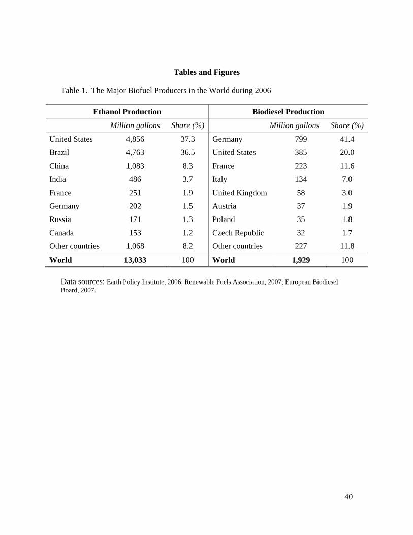
40

Tables and Figures Table 1. The Major Biofuel Producers in the World during 2006

Ethanol Production Biodiesel Production

Million gallons Share (%) Million gallons Share (%)

United States 4,856 37.3 Germany 799 41.4

Brazil 4,763 36.5 United States 385 20.0

China 1,083 8.3 France 223 11.6

India 486 3.7 Italy 134 7.0

France 251 1.9 United Kingdom 58 3.0

Germany 202 1.5 Austria 37 1.9

Russia 171 1.3 Poland 35 1.8

Canada 153 1.2 Czech Republic 32 1.7

Other countries 1,068 8.2 Other countries 227 11.8

World 13,033 100 World 1,929 100 Data sources: Earth Policy Institute, 2006; Renewable Fuels Association, 2007; European Biodiesel Board, 2007.

41

Table 2. Aggregation of Sectors and Regions used in the Model

No New Code Sector Description GTAP old sectors No. New Code Region Description Comprising GTAP old regions

1 CrGrains Cereal grains gro 1 USA United States usa

2 OthGrains Paddy and Wheat pdr wht 2 CAN Canada can

3 Oilseeds Oil seeds osd 3 EU27 European Union 27 aut bel dnk fin fra deu gbr grc irl ita lux nld prt esp swe bgr cyp cze hun mlt pol rom svk svn est lva ltu

4 Sugarcane Sugar cane, sugar beet c_b 4 BRAZIL Brazil bra

5 Livestock Cattle,Animal pdts,Milk,Wool ctl oap rmk wol 5 JAPAN Japan jpn

6 Forestry Forestry frs 6 CHIHKG China, Hong Kong chn hkg

7 Ethanol1 Ethanol1 (corn based) eth1 7 INDIA India ind

8 Ethanol2 Ethanol2 (sugarcane based) eth2 8 LAEEX Latin AmericanEnergy Exporters mex col ven arg

9 Biodiesel Biodiesel biod 9 RoLAC Rest of LatinAmerica+Caribbean xna per xap chl ury xsm xca xfa xcb

10 OthFoodPdts Other Food Products voln ofdn 10 EEFSUEX EE & FSU Energy Exp xef rus xsu

11 ProcLivestoc Meat, Dairy products cmt omt mil 11 RoE Rest of Europe che xer alb hrv tur

12 OthAgri other agriculture goods v_f pfb ocr pcr sgr b_t 12 MEASTNAEX Middle Eastern N Africa E Exp xme tun xnf bwa

13 OthPrimSect OtherPrimary:Fishery & Mining fsh omn 13 SSAEX Sub Saharan Energy Exporters xsc mwi moz tza zwe xsd mdg uga xss

14 Coal Coal coa 14 RoAFR Rest of North Africa & SSA mar zaf zmb

15 Oil Crude Oil oil 15 SASIAEEX South Asian Energy Exporters idn mys vnm xse

16 Gas Natural gas gas gdt 16 RoHIA Rest of High Income Asia kor twn

17 oil_pcts Petroleum, coal products p_c 17 RoASIA Rest of Southeast & South Asia xea phl sgp tha bgd lka xsa

18 electricity Electricity ely 18 Oceania Oceania countries aus nzl xoc

19 En_Int_Ind Energy intensive Industries crpn i_s nfm

20 Oth_Ind_Se Other industry and services tex wap lea lum ppp nmm fmp mvh otn ele ome omf wtr cns trd otp wtp atp cmn ofi isr obs ros osg dwe

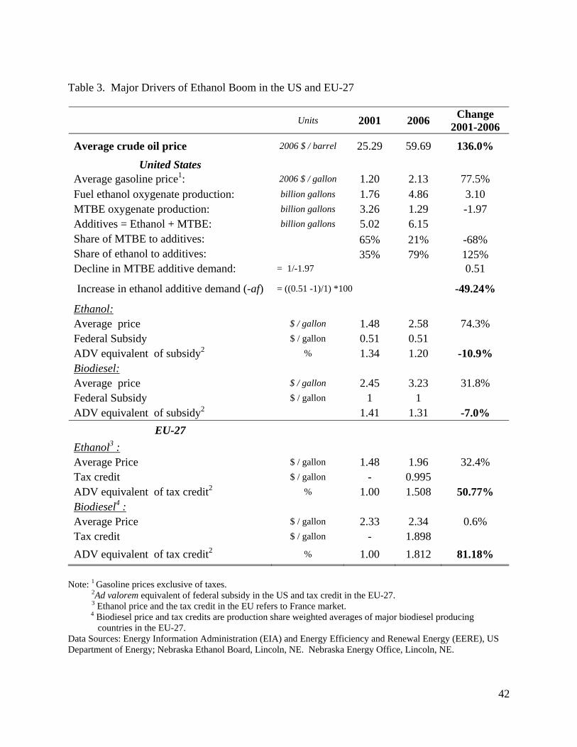
42

Table 3. Major Drivers of Ethanol Boom in the US and EU-27

Units 2001 2006 Change 2001-2006

Average crude oil price 2006 $ / barrel 25.29 59.69 136.0% United States

Average gasoline price1: 2006 $ / gallon 1.20 2.13 77.5% Fuel ethanol oxygenate production: billion gallons 1.76 4.86 3.10 MTBE oxygenate production: billion gallons 3.26 1.29 -1.97 Additives = Ethanol + MTBE: billion gallons 5.02 6.15 Share of MTBE to additives: 65% 21% -68% Share of ethanol to additives: 35% 79% 125% Decline in MTBE additive demand: = 1/-1.97 0.51

Increase in ethanol additive demand (-af) = ((0.51 -1)/1) *100 -49.24%

Ethanol: Average price $ / gallon 1.48 2.58 74.3% Federal Subsidy $ / gallon 0.51 0.51 ADV equivalent of subsidy2 % 1.34 1.20 -10.9% Biodiesel: Average price $ / gallon 2.45 3.23 31.8% Federal Subsidy $ / gallon 1 1 ADV equivalent of subsidy2 1.41 1.31 -7.0%

EU-27 Ethanol3 : Average Price $ / gallon 1.48 1.96 32.4% Tax credit $ / gallon - 0.995 ADV equivalent of tax credit2 % 1.00 1.508 50.77% Biodiesel4 : Average Price $ / gallon 2.33 2.34 0.6% Tax credit $ / gallon - 1.898 ADV equivalent of tax credit2 % 1.00 1.812 81.18%

Note: 1 Gasoline prices exclusive of taxes. 2Ad valorem equivalent of federal subsidy in the US and tax credit in the EU-27. 3 Ethanol price and the tax credit in the EU refers to France market. 4 Biodiesel price and tax credits are production share weighted averages of major biodiesel producing

countries in the EU-27. Data Sources: Energy Information Administration (EIA) and Energy Efficiency and Renewal Energy (EERE), US Department of Energy; Nebraska Ethanol Board, Lincoln, NE. Nebraska Energy Office, Lincoln, NE.

43

Table 4. Key Elasticities of Substitution in Biofuels and Land Use Module.

Regions ELHBIOIL Key Parameters Constant across all regions and sectors

US 3.95 Elasticity of substitution in Bio-Oil composite in production nest (ELBIOOIL)

0 Canada 2 EU-27 1.65 Brazil 1.35

Elasticity of substitution in AEZ production nest (ESAEZ) 20 Japan 2

China-Hong Kong 2 India 2

Scalar yield elasticity target (YDE_Target ) 0.4 Latin American Energy

Exporters 2

Rest of Latin America & Caribbean 2 Elasticity of transformation for

sluggish primary factor endowments (ETRAE)

-0.0001 EE & FSU Energy exporters 2

Rest of Europe 2 Elasticity of transformation for land cover at the bottom of land supply tree (ETRAE1)

-0.2 Middle Eastern N Africa energy exporters 2

Sub Saharan Energy exporters 2 Elasticity. of transformation for

crop land in supply tree (ETRAEL2)

-0.5 Rest of North Africa & SSA 2

South Asian Energy exporters 2

Rest of High Income Asia 2

Rest of Southeast & South Asia 2

Oceania countries 2

Note: ELHBIOIL refers to elasticity of substitution in Bio-Oil energy composite in private demand.

44

Table 5. Validation of the Model from Historical Evidence in the US, Brazil, and EU-27.

US.

Ethanol-1 Production

Million gallons

Model Prediction1:

Ethanol Production ($ million)

Corn Area Million hectares

Corn Production

Million tonnes

Model Prediction1:

Coarse Grain Production ($ million)

Share of Corn for Ethanol

Model Prediction1: Corn Share for Ethanol (% share)

Share of Corn for Exports

Model Prediction1: Corn Share for Exports

(% share)

2001 1770 2489.30 30.28 241.38 20936.5 6.5% 6.8% 19.4% 27.6% 2002 2130 31.56 227.77 7.5% 17.5% 2003 2800 31.44 256.28 11.0% 18.8% 2004 3400 32.37 299.92 11.7% 15.3% 2005 3900 32.71 282.31 14.5% 19.5% 2006 4855 6886.80 31.33 267.60 22335.0 20.2% 17.0% 20.5% 25.1%

2007* 7123 37.15 316.50 23.0% %Ch

2001-06 174.29 176.66 3.47 10.86 6.68 209.05 150.0 5.50 -9.06

%Ch 2000-07* 46.71 18.58 18.27

US Wheat Area

Million hectares

Wheat Production

Million tonnes

Rice Area Million hectares

Rice Production

Million tonnes

Model Prediction1: Other Grain Production ($ million)

Soybean Area Million hectares

Soybean Production

Million tonnes

Model Prediction1:

Oilseed Production ($ million)

Model Prediction1: Ch in Coarse Grain

exports ($ million)

2001 23.77 53.00 1.33 10.59 7304.8 29.63 78.67 12772.2 5779.3 2002 24.13 43.70 1.30 10.38 29.59 75.01 2003 24.86 63.81 1.21 9.84 29.36 66.78 2004 23.87 58.74 1.34 11.43 30.08 85.01 2005 22.89 57.28 1.35 10.99 28.86 84.00 2006 22.94 49.32 1.14 9.51 7070.8 30.21 86.69 12857.3 5601.1

2007* 25.63 71.30 %Ch

2001-06 -3.52 -6.95 -14.79 -10.21 -3.20 1.95 10.20 0.67 -3.08 %Ch

2000-07* -15.15 -17.75 Continued…

45

BRAZIL

Ethanol-2 Production

Million gallons

Model Prediction1:

Ethanol Production ($ million)

Sugarcane Area

Million hectares

Sugarcane Production:

Million tonnes

Model Prediction1: Sugarcane Production ($ million)

Share of Sugarcane for

Ethanol production

Model Prediction1: Sugarcane Share for Ethanol

Share of Sugarcane for Sugar

production

Model Prediction1: Sugarcane Share for

Sugar

Model Prediction1:

Ch in Ethanol-2 Exports

($ million) 2001 3609.0 5341.7 4.88 326.1 3189.4 43.3% 43.5% 55.7% 44.3% 137.7 2002 3760.0 5.02 344.3 45.2% 53.8% 2003 4336.0 5.1 363.7 46.2% 52.8% 2004 4443.0 5.5 416.6 49.1% 49.9% 2005 4467.0 5.69 421.8 53.0% 46.0% 2006 4491.0 7420.4 5.87 431.4 3737.4 51.0% 51.6% 48.0% 37.1% 970.7 %Ch

2001-06 24.44 38.91 20.29 32.29 17.18 17.67 18.51 -13.76 -16.29 604.88

EU-27

Biodiesel Production:

Million gallons

Model Prediction1: Biodiesel

Production ($ million)

Oilseeds Area:

Million hectares

Oilseeds Production:

Million tonnes

Model Prediction1:

Oilseed production ($ million)

Model Prediction1:

Oilseed Share for Biodiesel

Oilseed Imports: Million tonnes

Oilseed Exports: Million tonnes

Model Prediction1:

Ch in Oilseed imports

($ million)

Model Prediction1:

Ch in Oilseed exports

($ million)

2001 288 513.69 14.21 33.5 6905.1 6.50% 26.14 6.40 5440.41 1329.5 2002 384 14.13 31.5 25.27 6.76 2003 503 15.06 34.4 24.45 6.46 2004 708 14.83 38.6 21.69 7.00 2005 815 15.02 36.5 24.87 6.60 2006 1467 2729.56 15.82 37.9 8111.1 27.60% 28.05 6.19 5996.5 1243.9

%Ch 2001-06 409.38 431.37 11.3 13.1 17.47 324.62 7.29 -3.38 10.22 -6.44

Note: 1 Model prediction values refer to results from crude oil price in all regions, additive demand in the US, and biofuel subsidy shocks in the US and EU, performed together. The model predictions for 2001 are the pre-shock values (from the basedata) and 2006 values are post-shock values. Data Sources: Food and Agriculture Organization online database ; Economic Research Service, United States Dept of Agriculture; Renewable Fuels Association; European Biodiesel Board; The São Paulo Sugar Cane Agro-industry Union (UNICA).

46

Table 6. Impact of Biofuel Drivers on the Agricultural Production in the US, EU, and Brazil: 2001-2006 (% change in output by sector)

Total Change

(%)

Decomposed by Demand

Decomposed by Driver

Domestic Exports Additives Oil Price Subsidy-US Subsidy-EU US Ethanol-1 176.7 176.7 0.0 63.9 148.0 -34.9 -0.3 Coarse Grains 6.7 7.5 -0.9 2.4 5.6 -1.3 0.0 Other Grains -3.2 -0.5 -2.7 -1.1 -2.8 0.6 0.1 Oilseeds 0.7 0.1 0.6 -0.7 0.2 0.3 0.8 Sugarcane -0.9 -0.8 0.0 -0.2 -0.8 0.1 0.0 Other Agri -0.8 -0.7 -0.1 -0.2 -0.7 0.1 0.0 Livestock -1.2 -1.0 -0.1 -0.1 -1.1 0.1 0.0 Forestry -0.3 -0.3 0.0 -0.2 -0.3 0.1 0.0

EU-27

Biodiesel 431.4 431.4 0.0 -0.7 184.5 0.4 247.1 Coarse Grains 0.8 0.6 0.2 0.1 0.6 -0.1 0.2 Other Grains -1.1 -1.0 -0.1 0.1 -0.1 0.0 -1.1 Oilseeds 17.5 18.7 -1.2 0.2 7.8 -0.1 9.6 Sugarcane -0.5 -0.5 0.0 0.0 -0.2 0.0 -0.2 Other Agri -0.3 -0.6 0.3 0.0 0.0 0.0 -0.3 Livestock -0.5 -0.5 0.0 0.0 -0.4 0.0 -0.1 Forestry -1.5 -1.3 -0.2 0.0 -1.0 0.0 -0.5

Brazil

Ethanol-2 38.9 23.3 15.6 0.2 38.8 0.1 -0.2 Coarse Grains 0.7 -0.4 1.1 0.2 0.7 -0.1 -0.1 Other Grains 0.3 0.3 0.0 0.0 0.8 0.0 -0.5 Oilseeds 1.7 -0.5 2.2 0.2 -0.2 -0.2 1.8 Sugarcane 17.2 17.2 0.0 0.1 17.2 0.1 -0.1 Other Agri -1.8 -1.1 -0.7 0.0 -1.6 0.0 -0.1 Livestock 0.1 0.1 0.0 0.0 0.2 0.0 0.0 Forestry -2.0 -1.8 -0.2 0.0 -1.9 0.0 -0.1

47

Table 7. Impact of Biofuel Drivers on Market Price across Selected Regions: 2001-2006

% Change in Market Price

US EU-27 Brazil

Latin American

Energy Exporters

Middle Eastern North African

Energy Exporters

Sub- Saharan Energy

Exporters

Coarse Grains 8.68 6.98 5.9 6.32 13.54 10.03

Other Grains 6.35 6.39 5.43 6.77 12.63 9.04

Oilseeds 5.85 9.55 6.41 6.76 13.56 9.5

Sugarcane 5.08 5.48 10.96 5.81 14.47 9.07

Livestock 3.44 3.1 2.75 4.86 10.78 9.81

Forestry 4.19 7.00 8.29 5.13 17.77 16.71

Ethanol-1 16.87 -33.51 1.51 3.91 10.37 7.42

Ethanol-2 3.88 6.67 3.27 6.83 18.22 9.62

Biodiesel 12.75 -40.9 3.27 4.35 11.39 7.91

Other Food Products 1.92 -0.09 1.84 3.98 10.42 7.45

Processed Livestock 2.41 0.29 1.43 4.11 10.17 7.97

Other Agri Commodities 2.68 1.66 3.72 4.62 13.1 8.54

Other Primary sectors 2.62 3.27 3.44 5.51 11.69 8.55

Consumer Price Index (% ch) 2.99 2.71 3.01 5.40 12.22 8.93

48

Table 8. Change in Land Cover and Crop Area due to Biofuel Drivers: 2001-2006

Region Land Cover (% ch) Crop Harvested Area Change (%)

Crops Forest Pasture Coarse Grains Oilseeds Sugar-

cane Other Grains

Other Agri

US 1.3 -0.3 -0.4 5.0 -0.6 -2.0 -3.3 -1.2

Canada 0.8 -0.1 -0.1 1.4 -0.1 -0.4 0.8 0.1

EU-27 1.9 -1.1 -1.2 -0.4 15.0 -1.4 -2.1 -0.8

Brazil 2.8 -0.5 -0.4 -0.3 0.7 15.5 -1.0 -2.1

Japan 0.4 -0.1 0.0 3.9 1.4 -0.8 0.6 -0.7

China-Hong Kong 0.0 0.5 -0.2 0.0 2.0 -0.4 -0.5 -0.5

India 0.4 -0.6 -1.9 -0.7 0.0 -0.5 1.0 0.2

Latin American Energy Exporters -0.1 -0.2 0.1 0.9 -0.9 0.3 -0.1 -0.2

Rest of Latin America & Caribbean

0.8 0.1 -0.3 0.5 1.6 0.6 1.1 -0.4

EE & FSU Energy Exp -0.3 0.1 0.1 -0.7 1.1 -2.0 0.3 -0.3

Rest of Europe -0.2 0.7 -0.6 -0.7 0.7 -0.2 0.2 -0.2

Middle Eastern N Africa energy exporters

0.9 -2.0 -0.2 1.2 -1.1 1.1 -0.6 1.7

Sub Saharan Energy exporters -1.9 -0.5 0.7 1.2 -2.0 -0.8 -3.5 -1.7

Rest of North Africa & SSA 1.3 0.2 -0.3 -0.1 2.6 -0.3 2.1 -0.4

South Asian Energy exporters 0.3 -0.3 0.3 -0.1 0.7 -0.3 0.0 0.0

Rest of High Income Asia -0.4 0.2 -0.8 -0.4 3.4 -18.8 0.1 -0.9

Rest of Southeast & South Asia 0.8 -0.8 -0.3 -0.3 0.8 -0.6 0.5 -0.2

Oceania countries 1.1 -0.1 -0.1 1.6 2.7 -1.5 3.9 -1.6

49

Table 9. Impact of Biofuel Drivers on Bilateral Trade (change in import volume): 2001-2006 ($ millions)

Exporters: Coarse Grains Oilseeds Other Food Products

US EU RoW Total Exports US EU RoW Total

Exports US EU RoW Total Exports

1 US 0 -4 -174 -178 0 158 -81 77 0 -129 -85 -214

2 Canada 6 1 2 9 -3 19 -14 2 89 -9 14 93

3 EU-27 0 0 23 23 0 0 -130 -130 135 0 2667 2801

4 Brazil 0 4 22 26 0 179 -42 137 -8 -144 40 -112

5 Japan 0 0 0 0 0 0 0 1 8 -2 13 20

6 China-Hong Kong 0 1 40 42 1 49 52 102 29 -4 96 121 7 India 0 1 5 6 9 31 72 112 54 43 292 389

8 Latin American Energy Exporters 0 3 22 25 -2 23 -72 -51 -168 -347 -264 -779

9 Rest of Latin America & Caribbean 7 4 10 22 1 31 20 51 37 -41 110 106

10 EE & FSU Energy Exp 0 6 32 38 1 63 7 70 -19 -206 -170 -395 11 Rest of Europe 0 0 3 3 0 8 2 10 5 -28 105 82

12 Middle Eastern N Africa energy exporters -1 -2 -7 -9 -1 -7 -5 -13 -41 -191 -215 -447

13 Sub Saharan Energy exporters -1 -2 -4 -6 -1 -2 -20 -23 -19 -487 -154 -660 14 Rest of North Africa & SSA 0 1 19 20 0 4 3 8 -1 -39 89 49 15 South Asian Energy exporters 0 0 1 1 0 2 3 5 8 -54 42 -4 16 Rest of High Income Asia 0 0 0 0 0 0 0 1 -10 -10 -90 -111 17 Rest of Southeast & South Asia 0 0 6 6 0 2 15 17 138 8 251 398 18 Oceania countries 0 0 28 28 2 13 5 20 1 -14 -32 -45

Total 14 13 27 54 7 574 -185 395 238 -1654 2709 1293 Note: Change in volume of exports of coarse grains, oilseeds, and other food products, from all the 18 regions to the US and EU, respectively, were evaluated at initial market prices (trade volume changes in $ millions).

50

Table 10. Performance of Trade Balance due to Biofuel Drivers ($ billion).

Tra

ding

R

egio

ns

1 U

SA

2 C

AN

3 EU

27

4 B

RA

ZIL

5 JA

PAN

6 C

HIH

KG

7 IN

DIA

8 LA

EEX

9 R

oLA

C

10 E

EFSU

EX

11 R

oE

12 M

EAST

NA

EX

13 S

SAEX

14 R

oAFR

15 S

ASI

AEE

X

16 R

oHIA

17 R

oASI

A

18 O

cean

ia

Tota

l

Trading Sectors

Coarse Grains 0.26 0.02 0.04 0.07 -0.13 0.04 0.01 -0.01 0.00 0.05 0.00 -0.39 -0.02 0.02 -0.01 -0.02 0.01 0.05 -0.01

Other Grains 0.02 0.21 -0.04 -0.04 0.12 0.06 0.41 0.05 0.04 0.15 0.04 -1.47 -0.17 0.04 0.01 0.09 0.20 0.22 -0.06

Oilseeds 0.40 0.05 -0.89 0.32 -0.07 0.01 0.11 -0.04 0.07 0.08 0.01 -0.12 0.00 0.01 -0.01 -0.01 0.04 0.04 -0.03

Sugarcane 0.00 0.00 0.00 0.00 0.00 0.00 0.00 0.00 0.00 0.00 0.00 0.00 0.00 0.00 0.00 0.00 0.00 0.00 0.00

Livestock -0.16 0.09 -0.07 0.00 0.01 0.25 0.11 -0.08 0.03 -0.01 0.11 -0.49 -0.07 0.03 0.00 -0.02 0.07 0.14 -0.07

Forestry 0.04 -0.01 -0.13 0.00 -0.04 0.10 0.12 0.00 0.02 0.13 0.06 -0.07 -0.34 0.02 0.07 0.00 0.05 0.02 0.04

Ethanol-1 -0.02 0.02 0.00 0.00 0.00 0.00 0.00 0.00 0.00 0.00 0.00 0.00 0.00 0.00 0.00 0.00 0.00 0.00 0.00

Ethanol-2 -0.78 -0.07 -0.02 0.86 0.00 0.00 0.00 0.00 0.00 0.00 0.00 0.00 0.00 0.00 0.00 0.00 0.00 0.00 0.00

Biodiesel 0.00 0.00 0.00 0.00 0.00 0.00 0.00 0.00 0.00 0.00 0.00 0.00 0.00 0.00 0.00 0.00 0.00 0.00 0.00

Other Food Products -0.36 0.12 3.02 -0.04 0.09 0.23 0.45 -0.78 0.19 -0.57 0.13 -2.08 -1.07 0.09 0.06 -0.06 0.53 -

0.03 -0.08

Processed Livestock -0.76 0.21 2.28 0.24 0.19 0.27 0.23 -0.54 0.19 -0.29 0.16 -2.34 -0.57 0.06 0.09 0.02 0.37 0.06 -0.14

Other Agri Commodities -0.39 0.03 1.72 -0.02 0.18 0.45 0.75 -0.54 0.53 -0.34 0.51 -2.84 -1.75 0.20 0.06 0.22 1.06 0.05 -0.12

Oil & Oil Products -66.09 2.35 -62.45 -1.36 -29.29 -8.04 -8.24 29.20 -3.15 48.79 -6.18 115.12 20.09 -2.11 6.07 -18.34 -12.3 -1.45 2.64

Other Primary sectors -0.26 -0.56 4.37 0.24 0.72 -0.58 0.22 -0.34 0.22 -0.20 0.21 -2.62 -0.18 -0.66 -0.12 1.10 0.19 -1.05 0.71

Manufacturing & services -76.59 0.04 151.43 0.03 27.49 5.35 7.96 -41.35 1.49 -12.30 22.88 -99.38 -17.87 3.20 -4.90 18.43 11.37 -0.13 -2.88

Total -144.7 2.50 99.25 0.30 -0.74 -1.89 2.12 -14.4 -0.4 35.48 17.92 3.33 -1.97 0.89 1.32 1.42 1.62 -2.1 0.00

Note: For abbreviations of the regions, please refer to the corresponding serial numbers in Table 9.

51

Table 11. Decomposition of Terms of Trade for the US and EU ($ million).

US EU-27

World Price

Export Price

Import Price Total World

Price Export Price

Import Price Total

Coarse Grains 20 113 4 137 0 1 4 6 Other Grains -54 45 0 -9 -3 44 -19 22 Oilseeds -41 -7 2 -46 25 45 -28 43 Other Food Products -221 153 3 -65 258 -656 212 -186 Processed Livestock -316 161 -11 -166 -297 -256 174 -379 Other Agri Sectors -105 56 0 -49 429 -423 -25 -19 Biofuels 8 0 -12 -4 1 -16 16 1 Oil & Oil Products -53989 110 295 -53583 -76985 -133 -328 -77446

Other Primary sectors 457 26 -48 435 2948 -115 31 2864

Manufacturing & services -880 9462 -2518 6064 -7582 -20025 5575 -22032

Total -55122 10120 -2284 -47286 -81206 -21532 5612 -97126

52

Figure 1. World Production of Ethanol and Biodiesel (million gallons) (Data sources: Earth Policy Institute, 2006; FAPRI, 2007)

Figure 2. Modification of Consumption Structure in the GTAP-E Model

Household demand for private goods (CDE_COMM)

Energy Composite

CDE

Non-Energy Commodities

Coal Petroleum products & Biofuels composite

σELEGY = 0.1

Petro products (Oil_Pcts)

σELHBIOIL = 2 to 3.95

Biofuels (Ethanol1, Ethanol2, Biodiesel)

Oil Gas Electricity

CES

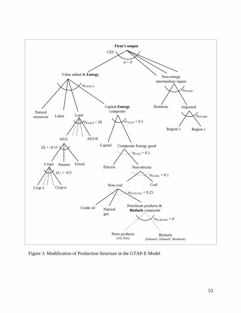
53

Figure 3. Modification of Production Structure in the GTAP-E Model

Firm’s output

Imported

Region r

Value added & Energy Non-energy intermediate inputs

σ= 0

σESUBD

Capital-Energy composite

σESUBVA

Land Labor

Region 1

Domestic

σESUBM

σ ELKE = 0.1

Non-electric

Capital

Electric

Coal

σELNEL = 0.1

Petroleum products & Biofuels compositeCrude oil

σELNCOAL = 0.25

Non-coal

Petro products (Oil_Pcts)

σELBIOOIL = 0

Biofuels (Ethanol1, Ethanol2, Biodiesel)

Composite Energy good

σELEN = 0.1

Natural gas

AEZi AEZ18

σESAEZ = 20

CES

Ω1 = -0.11

Crops Pasture Forest

Crop-1 Crop-n

Ω 2 = -0.5

Natural resources

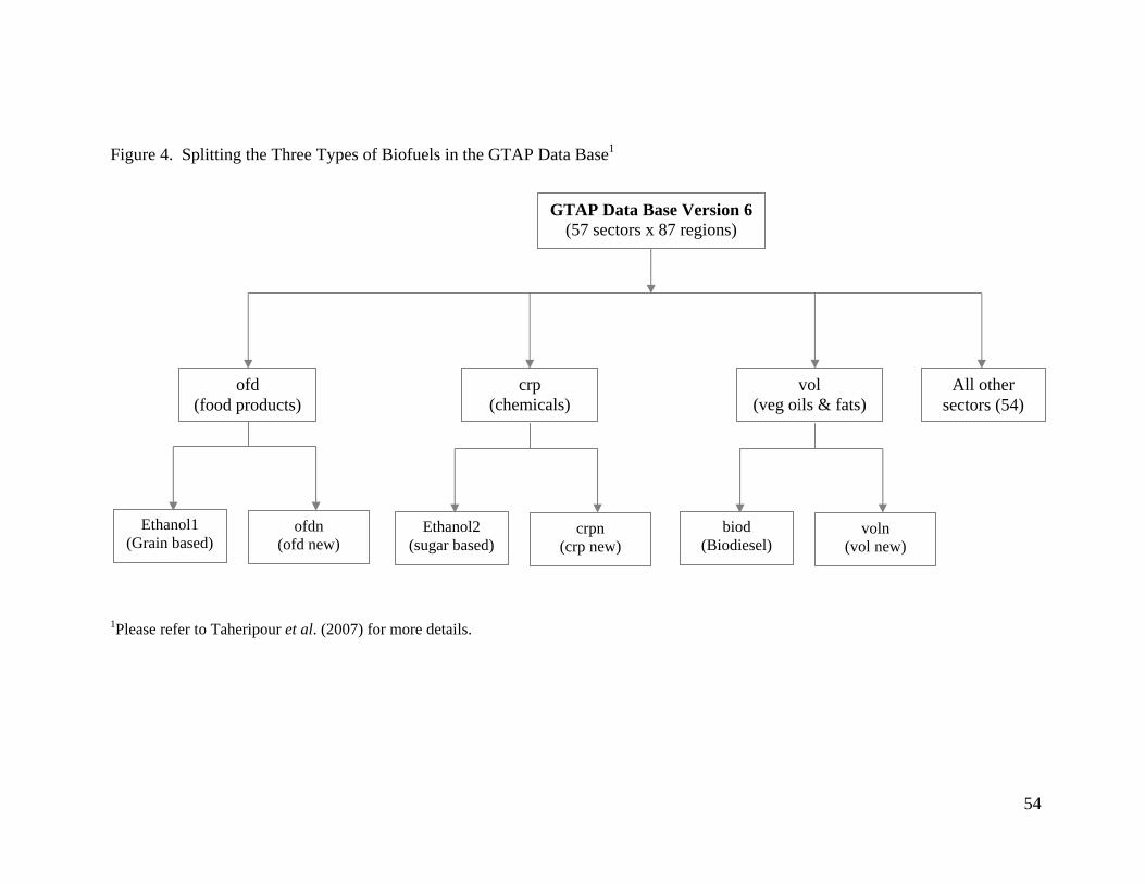
54

Figure 4. Splitting the Three Types of Biofuels in the GTAP Data Base1

1Please refer to Taheripour et al. (2007) for more details.

GTAP Data Base Version 6 (57 sectors x 87 regions)

ofd (food products)

crp (chemicals)

vol (veg oils & fats)

All other sectors (54)

ofdn (ofd new)

Ethanol1 (Grain based)

crpn (crp new)

Ethanol2 (sugar based)

voln (vol new)

biod (Biodiesel)

55

-10.46 (minimum)-0.090.74 (median)1.648.17 (maximum)

% Change in Land Area under Coarse Grains: 2001-2006

Figure 5. Change in Land Area across AEZs under Coarse Grains: 2001-2006.

-2.17 (minimum)0.051.20 (median)2.3619.17 (maximum)

% Change in Land Area under Oilseeds: 2001-2006

Figure 6. Change in Land Area across AEZs under Oilseeds: 2001-2006.

56

-11.47 (minimum)-0.51-0.12 (median)0.4918.74 (maximum)

% Change in Land Area under Sugarcane: 2001-2006

Figure 7. Change in Land Area across AEZs under Sugar Crops: 2001-2006.

-12.02 (minimum)-0.260.43 (median)1.356.34 (maximum)

% Change in Land Area under Other Grains: 2001-2006

Figure 8. Change in Land Area across AEZs under Other Grains (Paddy & Wheat): 2001-06.

57

-10.89 (minimum)-0.31-0.09 (median)0.242.63 (maximum)

% Change in Land Area under Other Agri : 2001-2006

Figure 9. Change in Land Area across AEZs under Other Agri Goods: 2001-2006.

-6.92 (minimum)-0.94-0.45 (median)0.061.33 (maximum)

% Change in Land Area under Forest: 2001-2006

Figure 10. Change in Land Area across AEZs under Forestry: 2001-2006.

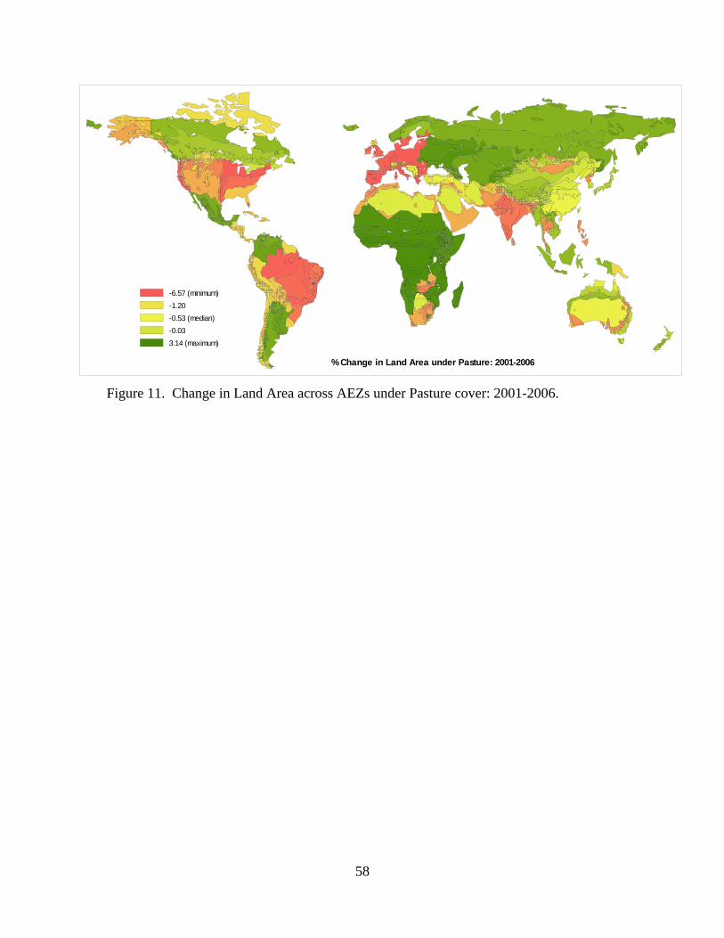
58

-6.57 (minimum)-1.20-0.53 (median)-0.033.14 (maximum)

% Change in Land Area under Pasture: 2001-2006

Figure 11. Change in Land Area across AEZs under Pasture cover: 2001-2006.

59

Appendix-1: Closure and Shocks for Analyzing the Impact of Biofuel Boom

! Oil Price, Additive, to - Shocks closure exogenous afall afcom afreg afsec ams aoall aoreg aosec atd atf atm ats au cgdslack dpgov dppriv dpsave endwslack incomeslack pemp pfactwld pop profitslack psaveslack qo(ENDW_COMM,REG) RCTAXB tm tms to tpd tpm tp tradslack tx txs ; Rest Endogenous ; swap aosec("oil") = pxwcom("oil");

List of Shocks: Shock pxwcom("oil") = 136; Shock afall("ethanol1","Oil_pcts","USA") = -49; Shock to("Ethanol1","USA") = -10.93; Shock to("biodiesel","USA") = -7.00; Shock to("Ethanol1","EU27") = 50.77; Shock to("biodiesel","EU27") = 81.18; Subtotal afall = MTBE ban ; Subtotal pxwcom = World oil price ; Subtotal to(NSAV_COMM,"USA") = USA subsidies ; Subtotal to(NSAV_COMM,"EU27") = EU subsidies ;