IMPACT OF AGGREGATED WIND OUTPUT ON WIND INTEGRATION COSTS

Samir Succar, Energy Analyst, Natural Resources Defense Council, 40 W20th St, New York, NY 10011

Phone: +1 212 727 4536, E-mail: ssuccar@nrdc.org

OVERVIEW As the penetration of wind on the grid continues to increase, new adaptive strategies will be required to integrate large quantities of variable generation. Although wind still provides less than 2% of total US generation [1], cumulative capacity continues to grow rapidly with penetrations reaching 5-8% in a handful of states [2]. The fluctuations in wind power output do not impose substantial balancing costs on the system when wind provides only a small fraction of total generation, but as penetrations reach 10-20% the integration costs become significant [3]. The magnitude of these costs depends on the generation mix, size of balancing area and strength of the regional transmission system, but it is clear that even under ideal conditions, active balancing and even direct backup of wind will be required as wind penetrations reach very high levels [4].

The use of storage to balance wind addresses both the variability and remoteness of wind [5-8]. Bulk storage enables wind to provide dispatchable power and mitigates the impact of temporal fluctuations inherent in the resource. In addition, the delivery of power at high capacity factors enables increased utilization of long distance transmission lines that deliver remote wind to market. This method of balancing wind to provide baseload power can be compared with direct backup of wind using local generation from natural gas fired capacity.

The backup requirements needed to provide baseload power from wind depend critically on the variability of the wind resource. Aggregation of multiple wind sites over a broad geographic region can substantially mitigate this variability by reducing the frequency of both high and low wind speed events [9]. This paper will investigate the impacts of this resource aggregation on the backup requirements for producing baseload power from.

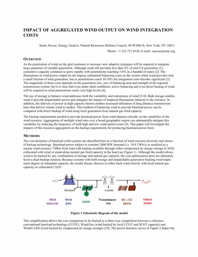
METHODS The cost dynamics of baseload wind systems are described here as a function of wind resource diversity and choice of backup technology. Baseload power subject to constant 2000 MW demand (i.e. 14.9 TWh/y) is modeled as a remote wind resource 750km from load with backup available through either compressed air energy storage (CAES) collocated with wind or stand-alone natural gas fired capacity at the load (see Figure 1). Although the model allows wind to be backed by any combination of storage and natural gas capacity, the cost optimization does not ultimately favor a dual-backup solution. Because systems with both storage and dispatchable generation backing wind imply some degree of redundant capacity, the model always chooses to either back wind entirely with local natural gas capacity or collocated CAES.

Figure 1 Schematic diagram of the model

This simplification allows the cost comparison to be framed as a three-way competition between a reference conventional baseload technology (CCGT), Wind/Gas (wind backed by local CCGT and SCGT capacity) and Wind/CAES (wind backed by compressed air energy storage) [10]. The power duration curves in Figure 2 depict the

sources of power and cumulative output for these three systems, each of which is constrained to deliver a minimum capacity factor of 85%. The natural gas fired generation is local to load and it is assumed that wind and CAES are collocated and served by a 750km, 500kV HVDC transmission line (see Table 1 for base case modeling assumptions and Table 2 for model cost equations).

The power duration curves presented in this nominal case use the output of a synthetic Rayleigh-distributed hourly wind speed time series and optimize the wind and backup components with respect to the levelized cost of energy [10-12].

The result of this optimization provides three baseload systems that rely on a combination of wind and natural gas to deliver baseload power. Because the heat rate of the storage system is relatively low (4220 versus 6700 kJ LHV/kWh for CCGT) and because Wind/CAES delivers the largest fraction of its power from wind directly, this system represents the plant with the lowest greenhouse gas (GHG) emission rate of the three considered here (108 gCO2/kWh). By comparison, the CCGT option has a GHG emission rate of approximately 440 gCO2/kWh, while Wind/Gas generates 256 gCO2/kWh. The result is a cost of energy competition between the three systems that depends on the price of fuel, or alternatively GHG emissions price.

Figure 2 Power duration curves for three alternative baseload systems: CCGT (top left), Wind/Gas (top right), Wind/CAES (bottom left), N=1

Figure 3 Levelized cost of energy for Gas (CCGT/SCGT), Wind/Gas (Wind backed by CCGT/SCGT) and Wind/CAES (wind backed by compressed air energy storage)

Because all the systems in this analysis use natural gas as their fuel, changes in GHG emissions price pGHG (with a constant, nominal fuel price pNG=$6.0/GJ HHV [13]) can be equivalently expressed in terms of changes in fuel price pNG (with a constant, nominal GHG emissions price pGHG=$0/tCe). The equivalence between pNG and pGHG is established by the nominal value of each parameter and the greenhouse gas emissions intensity of the fuel. The value used here is the sum of the carbon content of natural gas (55.6kg CO2/GJ LHV [13]) and the upstream emission rate (10.4 kgCO2/GJ LHV [14]), which means a $30/tCO2 increase in pGHG is equivalent to an “effective” fuel price increase of $1.78/GJ HHV. Thus, we can describe changes in effective fuel price either in terms of pGHG or pNG.

The cost of energy of these baseload systems is shown in Figure 3 as a function of the effective fuel price. Because the optimal configuration for each system is constant with respect to fuel price, the cost curve for each technology is linear. The crossing points or “entry price” for Wind/Gas and Wind/CAES at which they become the lowest cost option is $102/tCO2 ($12.1/GJ) and $148/tCO2 ($14.8/GJ) respectively (see Figure 3).

The aggregation of wind over a broad geographic area provides an alternative method of mitigating the variability in wind. While the fluctuations imposed by wind at a single site can impose substantial ramping events on the system, pooling multiple weakly correlated geographically distributed wind resources can smooth the overall profile of the wind substantially [15-17].

Since weakly correlated wind resources will rarely experience simultaneous gusts, the combined output from multiple farms will rarely reach the rated output of the combined wind system. As a result, the left-hand peak of the wind power duration curve will narrow as the number of wind resources (N) increases (see Figure 4). In addition, the knee of power duration curve will be raised and shifted rightward with increasing numbers of wind turbine arrays since the aggregated wind resources will likewise rarely experience simultaneous lulls. The results of these changes in the power duration curve are depicted in Figure 4 for N=1, 2, 4, 8 and 16.

The narrowed peak of the power duration curve reduces the curtailment penalty of increasing the size of the total wind nameplate capacity above the transmission line capacity (i.e. over-sizing the wind turbine array). Furthermore, the broadening of the base means that the wind can guarantee a higher capacity for a larger fraction of the time. Therefore large numbers of wind turbine arrays aggregated over a broad region could enable wind to achieve a greater capacity credit, reduce reserve requirements on the system and in the limit of high values of N, produce a degree of baseload power without backup [15].

In this case, each wind turbine array is a separate, independently generated synthetic wind speed time series and therefore the results of the model will reflect a greater diversity benefit from aggregating wind than would be realized by pooling wind across a somewhat limited region with more strongly correlated wind resources. In this regard, the overall trends are more important that the specific N values at which the data points are presented.

Figure 4 Power duration curve from wind, showing the impact of pooling aggregated output from 1, 2, 4, 8 and 16 wind turbine arrays (N). Vertical axis is power output, normalized so that the combined rated capacity of the arrays = 1.0

RESULTS Incorporating wind resource aggregation into the baseload wind cost optimization model facilitates an analysis of combined wind integration strategies for providing dispatchable power from wind. The change in wind resource characteristics has an important impact on both the Wind/Gas and Wind/CAES systems configuration and might reduce the backup requirements needed to meet baseload power requirements. Therefore this combined approach of both mitigating wind variability through resource aggregation and firming output with backup capacity might result in super-additive cost benefits for baseload wind systems in this analysis and for wind integration more broadly.

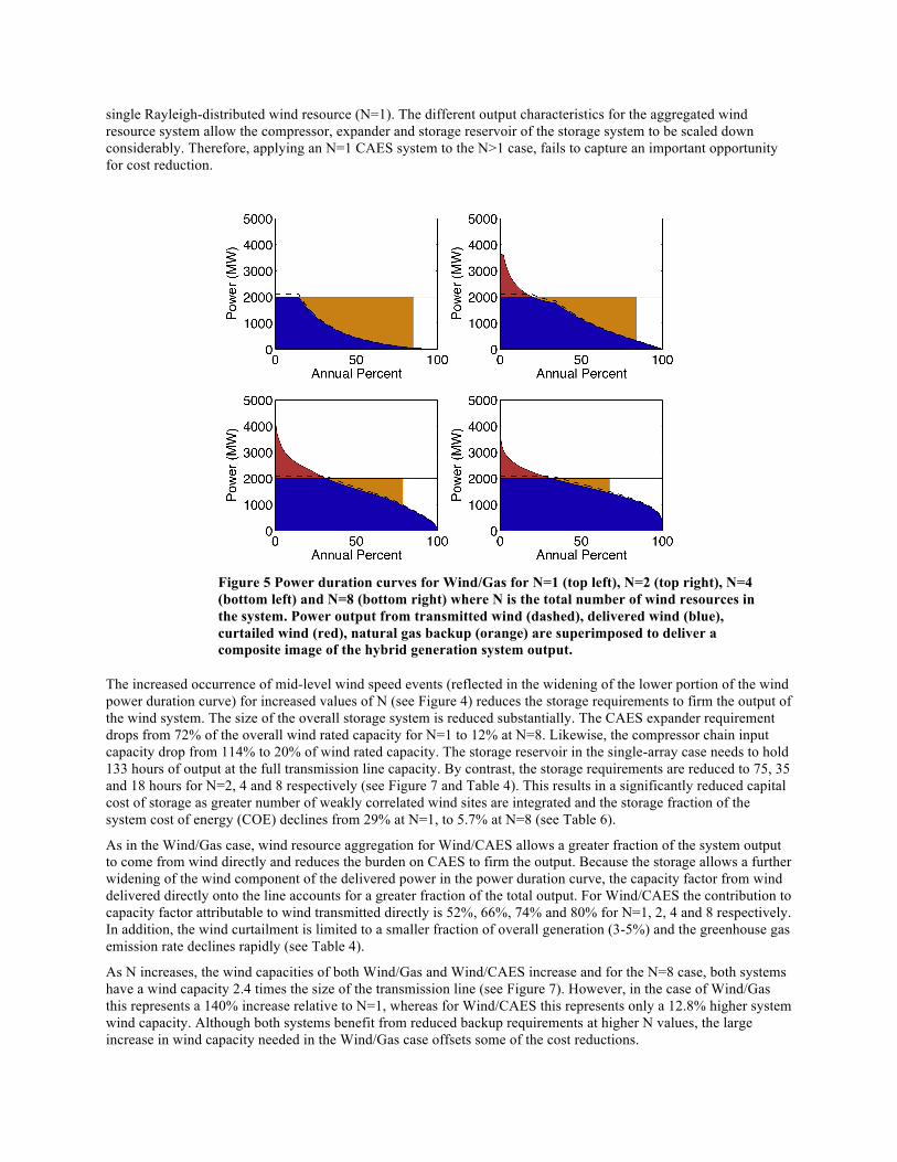
For the N=1 case, the rated capacity of the wind turbine array in the Wind/Gas system was matched to the transmission line capacity in order to minimize wind curtailment (see Figure 2). However, as the system takes advantage of greater resource diversity, the wind output can be increasingly oversized with respect to the line at minimal curtailment penalty (see Figure 5 and Table 3). By comparison, for the N=8 case, the wind capacity can be sized to 2.4 times the transmission line with 6.8% curtailment.

The over-sizing of the wind system enhances the utilization of the long distance transmission line since a greater fraction of the full system output comes from the remote wind rather than the local natural gas backup. In this case transmission line capacity factor increases from 36% for a single wind site, to 56%, 73% and 80% for N = 2, 4 and 8 respectively (curtailed output accounted for 6-10% of delivered energy). Because resource aggregation enables a greater fraction of the 85% capacity factor to be delivered from wind and reduces reliance on backup generation, it also enables a steep reduction in greenhouse gas emissions for the system as a whole (see Figure 7 and Table 3).

Combining the output from multiple wind resources also has important impacts on the Wind/CAES system. Although prior studies have suggested that CAES is not economic on the system when wind resources are pooled over a large region [7], these results do not capture the benefits of re-optimizing the storage system for changing wind resource dynamics. The storage system for the Wind/CAES system described above is optimized for backing a

single Rayleigh-distributed wind resource (N=1). The different output characteristics for the aggregated wind resource system allow the compressor, expander and storage reservoir of the storage system to be scaled down considerably. Therefore, applying an N=1 CAES system to the N>1 case, fails to capture an important opportunity for cost reduction.

Figure 5 Power duration curves for Wind/Gas for N=1 (top left), N=2 (top right), N=4 (bottom left) and N=8 (bottom right) where N is the total number of wind resources in the system. Power output from transmitted wind (dashed), delivered wind (blue), curtailed wind (red), natural gas backup (orange) are superimposed to deliver a composite image of the hybrid generation system output.

The increased occurrence of mid-level wind speed events (reflected in the widening of the lower portion of the wind power duration curve) for increased values of N (see Figure 4) reduces the storage requirements to firm the output of the wind system. The size of the overall storage system is reduced substantially. The CAES expander requirement drops from 72% of the overall wind rated capacity for N=1 to 12% at N=8. Likewise, the compressor chain input capacity drop from 114% to 20% of wind rated capacity. The storage reservoir in the single-array case needs to hold 133 hours of output at the full transmission line capacity. By contrast, the storage requirements are reduced to 75, 35 and 18 hours for N=2, 4 and 8 respectively (see Figure 7 and Table 4). This results in a significantly reduced capital cost of storage as greater number of weakly correlated wind sites are integrated and the storage fraction of the system cost of energy (COE) declines from 29% at N=1, to 5.7% at N=8 (see Table 6).

As in the Wind/Gas case, wind resource aggregation for Wind/CAES allows a greater fraction of the system output to come from wind directly and reduces the burden on CAES to firm the output. Because the storage allows a further widening of the wind component of the delivered power in the power duration curve, the capacity factor from wind delivered directly onto the line accounts for a greater fraction of the total output. For Wind/CAES the contribution to capacity factor attributable to wind transmitted directly is 52%, 66%, 74% and 80% for N=1, 2, 4 and 8 respectively. In addition, the wind curtailment is limited to a smaller fraction of overall generation (3-5%) and the greenhouse gas emission rate declines rapidly (see Table 4).

As N increases, the wind capacities of both Wind/Gas and Wind/CAES increase and for the N=8 case, both systems have a wind capacity 2.4 times the size of the transmission line (see Figure 7). However, in the case of Wind/Gas this represents a 140% increase relative to N=1, whereas for Wind/CAES this represents only a 12.8% higher system wind capacity. Although both systems benefit from reduced backup requirements at higher N values, the large increase in wind capacity needed in the Wind/Gas case offsets some of the cost reductions.

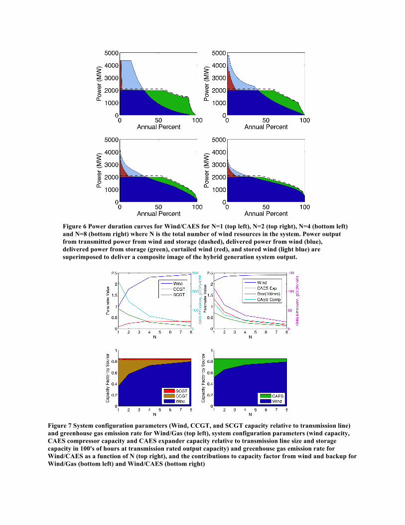
Figure 6 Power duration curves for Wind/CAES for N=1 (top left), N=2 (top right), N=4 (bottom left) and N=8 (bottom right) where N is the total number of wind resources in the system. Power output from transmitted power from wind and storage (dashed), delivered power from wind (blue), delivered power from storage (green), curtailed wind (red), and stored wind (light blue) are superimposed to deliver a composite image of the hybrid generation system output.

Figure 7 System configuration parameters (Wind, CCGT, and SCGT capacity relative to transmission line) and greenhouse gas emission rate for Wind/Gas (top left), system configuration parameters (wind capacity, CAES compressor capacity and CAES expander capacity relative to transmission line size and storage capacity in 100's of hours at transmission rated output capacity) and greenhouse gas emission rate for Wind/CAES as a function of N (top right), and the contributions to capacity factor from wind and backup for Wind/Gas (bottom left) and Wind/CAES (bottom right)

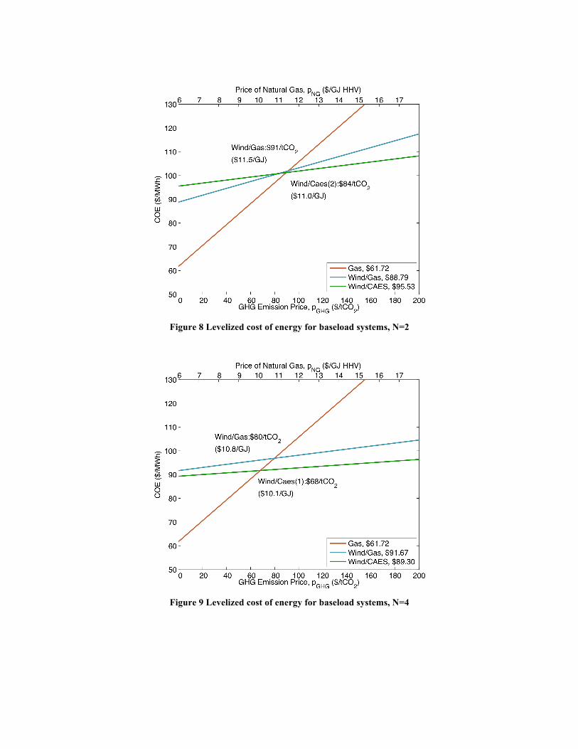
Figure 8 Levelized cost of energy for baseload systems, N=2

Figure 9 Levelized cost of energy for baseload systems, N=4

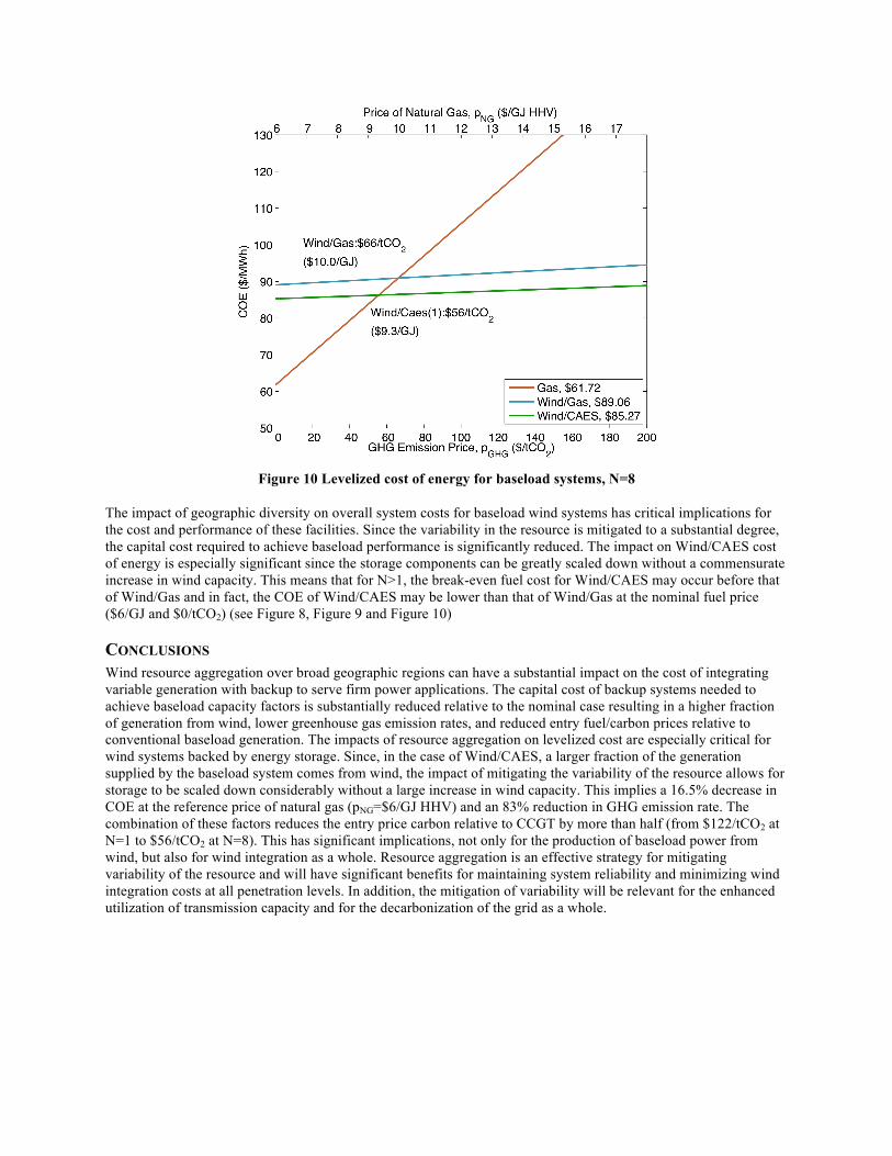
Figure 10 Levelized cost of energy for baseload systems, N=8

The impact of geographic diversity on overall system costs for baseload wind systems has critical implications for the cost and performance of these facilities. Since the variability in the resource is mitigated to a substantial degree, the capital cost required to achieve baseload performance is significantly reduced. The impact on Wind/CAES cost of energy is especially significant since the storage components can be greatly scaled down without a commensurate increase in wind capacity. This means that for N>1, the break-even fuel cost for Wind/CAES may occur before that of Wind/Gas and in fact, the COE of Wind/CAES may be lower than that of Wind/Gas at the nominal fuel price ($6/GJ and $0/tCO2) (see Figure 8, Figure 9 and Figure 10)

CONCLUSIONS Wind resource aggregation over broad geographic regions can have a substantial impact on the cost of integrating variable generation with backup to serve firm power applications. The capital cost of backup systems needed to achieve baseload capacity factors is substantially reduced relative to the nominal case resulting in a higher fraction of generation from wind, lower greenhouse gas emission rates, and reduced entry fuel/carbon prices relative to conventional baseload generation. The impacts of resource aggregation on levelized cost are especially critical for wind systems backed by energy storage. Since, in the case of Wind/CAES, a larger fraction of the generation supplied by the baseload system comes from wind, the impact of mitigating the variability of the resource allows for storage to be scaled down considerably without a large increase in wind capacity. This implies a 16.5% decrease in COE at the reference price of natural gas (pNG=$6/GJ HHV) and an 83% reduction in GHG emission rate. The combination of these factors reduces the entry price carbon relative to CCGT by more than half (from $122/tCO2 at N=1 to $56/tCO2 at N=8). This has significant implications, not only for the production of baseload power from wind, but also for wind integration as a whole. Resource aggregation is an effective strategy for mitigating variability of the resource and will have significant benefits for maintaining system reliability and minimizing wind integration costs at all penetration levels. In addition, the mitigation of variability will be relevant for the enhanced utilization of transmission capacity and for the decarbonization of the grid as a whole.

REFERENCES [1] EIA, "Annual Energy Outlook 2009 With Projections to 2030," Office of Integrated Analysis and Forecasting,

Energy Information Administration, US Department of Energy, Washington, D.C. DOE/EIA-0383(2009) March 2009.

[2] AWEA, "WINDPOWER OUTLOOK 2009," American Wind Energy Association, Washington, DC 2009. [3] H. Holttinen, B. Lemström, P. Meibom, H. Bindner, A. Orths, F. v. Hulle, C. Ensslin, L. Hofmann, W. Winter,

A. Tuohy, M. O’Malley, P. Smith, J. Pierik, J. O. Tande, A. Estanqueiro, J. Ricardo, E. Gomez, L. Söder, G. Strbac, A. Shakoor, J. C. Smith, B. Parsons, M. Milligan, and Y.-h. Wan, "Design and operation of power systems with large amounts of wind power: State-of-the-art report " VTT Technical Research Centre of Finland, Vuorimiehentie, Finland VTT–WORK–82, October 2007.

[4] DENA Project Steering Group, "Planning of the Grid Integration of Wind Energy in Germany Onshore and Offshore up to the Year 2020 (DENA Grid study)," Deutsche Energie-Agentur, Berlin March 15 2005.

[5] A. J. Cavallo, "High-capacity factor wind energy systems," Journal of Solar Energy Engineering, Transactions of the ASME, vol. 117, pp. 137-143, 1995.

[6] B. Sorensen, "Fluctuating Power-Generation of Large Wind Energy Converters, with and without Storage Facilities," Solar Energy, vol. 20, pp. 321-331, 1978.

[7] J. F. DeCarolis and D. W. Keith, "The economics of large-scale wind power in a carbon constrained world," Energy Policy, vol. 34, pp. 395-410, Mar 2006.

[8] J. V. Paatero and P. D. Lund, "Effect of energy storage on variations in wind power," Wind Energy, vol. 8, pp. 421-441, Oct-Dec 2005.

[9] IEA, "Variability of Wind Power and other Renewables: Management Options and Strategies," International Energy Agency, Paris, France June 2005.

[10] J. B. Greenblatt, S. Succar, D. C. Denkenberger, R. H. Williams, and R. H. Socolow, "Baseload wind energy: modeling the competition between gas turbines and compressed air energy storage for supplemental generation," Energy Policy, vol. 35, pp. 1474-1492, Mar 2007.

[11] A. R. McFarlane, P. S. Veers, and L. L. Schluter, "Simulating high frequency wind for long durations," in Proceedings of the Energy-Sources Technology Conference, New Orleans, LA, USA, 1994, pp. 175-180.

[12] A. J. Cavallo and M. B. Keck, "Cost effective seasonal storage of wind energy," Houston, TX, USA, 1995, pp. 119-125.

[13] EIA, "Annual Energy Outlook 2007 With Projections to 2030," Office of Integrated Analysis and Forecasting, Energy Information Administration, US Department of Energy, Washington, D.C. DOE/EIA-0383(2007), February 2007.

[14] M. Q. Wang, "GREET 1.5 - Transport Fuel-Cycle Model," Center for Transporation Research, Energy Systems Division, Argonne Natinoal Laboratory, Argonne, IL ANL/ESD-39, Vol. 2, August 1999.

[15] C. L. Archer and M. Z. Jacobson, "Supplying baseload power and reducing transmission requirements by interconnecting wind farms," Journal of Applied Meteorology and Climatology, vol. 46, pp. 1701-1717, 2007.

[16] P. Nørgaard, "MAWIPOC - A Model to Simulate the Aggregated Wind Power Time Series For an Area," in European Wind Energy Conference EWEC '04 London, UK, 2004.

[17] J. Soens, J. Driesen, and R. Belmans, "Estimation of Fluctuation of Wind Power Generation in Belgium," in Fifth International Workshop On Large-Scale Integration Of Wind Power And Transmission Networks For Offshore Wind Farms Glasgow, 2005.

[18] D. J. Malcolm and A. C. Hansen, "WindPACT turbine rotor design study," National Renewable Energy Laboratory, Golden, CO 2002.

[19] EPRI, "Technical Assessment Guide (TAG)," Electric Power Research Institute, Palo Alto, CA TR-102275, 1993.

[20] D. Denkenberger, "Optimal wind turbine rated speed taking into account array effects, the larger system, and climate impacts.," in Department of Mechanical and Aerospace Engineering. vol. Master of Science and Engineering Princeton, NJ: Princeton University, 2005.

[21] R. Wiser and M. Bolinger, "Annual Report on U.S. Wind Power Installation, Cost, and Performance Trends: 2006," U.S. Department of Energy, Energy Efficiency and Renewable Energy, Washington, D.C. DOE/GO-102007-2433, May 2007.

[22] EPRI-DOE, "Handbook of Energy Storage for Transmission and Distribution Applications," EPRI, DOE, Palo Alto, CA, Washington, DC 2003.

[23] EPRI-DOE, "Energy Storage for Grid Connected Wind Generation Applications," EPRI, DOE, Palo Alto, CA, Washington, DC 1008703, 2004.

[24] M. Nakhamkin, R. H. Wolk, S. van der Linden, and M. Pate, "New compressed air energy storage concept improves the profitability of existing simple cycle, combined cycle, wind energy, and landfill gas power plants," Vienna, Austria, 2004, pp. 103-110.

[25] M. P. Bahrman and B. K. Johnson, "The ABCs of HVDC transmission technologies," IEEE Power & Energy Magazine, vol. 5, pp. 32-44, 2007.

[26] M. Szechtman, P. S. Maruvada, and R. N. Nayak, "800-kV HVDC on the horizon," IEEE Power & Energy Magazine, vol. 5, pp. 61-9, 2007.

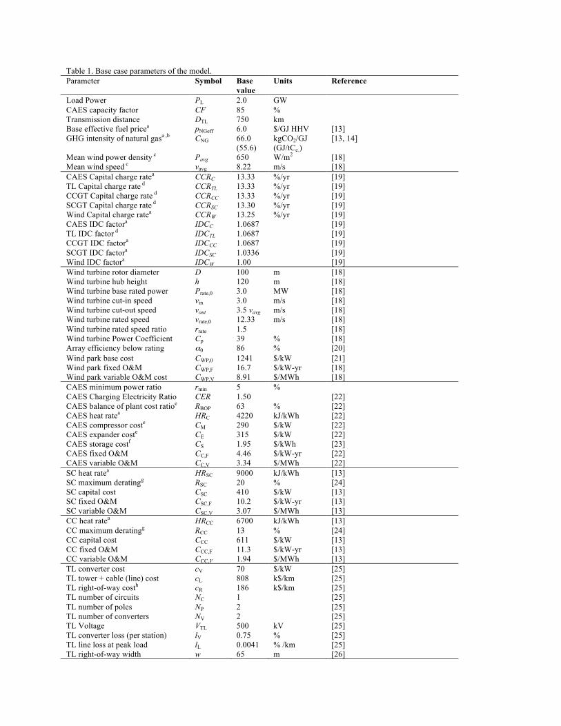
Table 1. Base case parameters of the model. Parameter Symbol Base

value Units Reference

Load Power PL 2.0 GW CAES capacity factor CF 85 % Transmission distance DTL 750 km Base effective fuel pricea pNGeff 6.0 $/GJ HHV [13] GHG intensity of natural gasa ,b CNG 66.0

(55.6) kgCO2/GJ (GJ/tCe.)

[13, 14]

Mean wind power density c Pavg 650 W/m2 [18] Mean wind speed c vavg 8.22 m/s [18] CAES Capital charge ratea CCRC 13.33 %/yr [19] TL Capital charge rate d CCRTL 13.33 %/yr [19] CCGT Capital charge rate d CCRCC 13.33 %/yr [19] SCGT Capital charge rate d CCRSC 13.30 %/yr [19] Wind Capital charge ratea CCRW 13.25 %/yr [19] CAES IDC factora IDCC 1.0687 [19] TL IDC factor d IDCTL 1.0687 [19] CCGT IDC factora IDCCC 1.0687 [19] SCGT IDC factora IDCSC 1.0336 [19] Wind IDC factora IDCW 1.00 [19] Wind turbine rotor diameter D 100 m [18] Wind turbine hub height h 120 m [18] Wind turbine base rated power Prate,0 3.0 MW [18] Wind turbine cut-in speed vin 3.0 m/s [18] Wind turbine cut-out speed vout 3.5 vavg m/s [18] Wind turbine rated speed vrate,0 12.33 m/s [18] Wind turbine rated speed ratio rrate 1.5 [18] Wind turbine Power Coefficient Cp 39 % [18] Array efficiency below rating α0 86 % [20] Wind park base cost CWP,0 1241 $/kW [21] Wind park fixed O&M CWP,F 16.7 $/kW-yr [18] Wind park variable O&M cost CWP,V 8.91 $/MWh [18] CAES minimum power ratio rmin 5 % CAES Charging Electricity Ratio CER 1.50 [22] CAES balance of plant cost ratioe RBOP 63 % [22] CAES heat ratea HRC 4220 kJ/kWh [22] CAES compressor coste CM 290 $/kW [22] CAES expander coste CE 315 $/kW [22] CAES storage costf CS 1.95 $/kWh [23] CAES fixed O&M CC,F 4.46 $/kW-yr [22] CAES variable O&M CC,V 3.34 $/MWh [22] SC heat ratea HRSC 9000 kJ/kWh [13] SC maximum deratingg RSC 20 % [24] SC capital cost CSC 410 $/kW [13] SC fixed O&M CSC,F 10.2 $/kW-yr [13] SC variable O&M CSC,V 3.07 $/MWh [13] CC heat ratea HRCC 6700 kJ/kWh [13] CC maximum deratingg RCC 13 % [24] CC capital cost CCC 611 $/kW [13] CC fixed O&M CCC,F 11.3 $/kW-yr [13] CC variable O&M CCC,V 1.94 $/MWh [13] TL converter cost cV 70 $/kW [25] TL tower + cable (line) cost cL 808 k$/km [25] TL right-of-way costh cR 186 k$/km [25] TL number of circuits NC 1 [25] TL number of poles NP 2 [25] TL number of converters NV 2 [25] TL Voltage VTL 500 kV [25] TL converter loss (per station) lV 0.75 % [25] TL line loss at peak load lL 0.0041 % /km [25] TL right-of-way width w 65 m [26]

a Thermal content stated in LHV basis, except energy prices are on a higher heating value (HHV) basis—the norm for US energy pricing.

b Natural gas carbon dioxide content of 55.6 kgCO2/GJ LHV [13] and upstream GHG emissions (10.4 kgCO2/GJ LHV) [14].

c Extrapolated from 10 m reference Class 4 wind speed (5.77 m/s) using 1/7 scaling exponent to assumed hub height of 120 m.

d Obtained from EPRI accounting rules [19] with the following assumptions: construction period for CAES, CCGT and TL of 3 years (3 equal payments), construction period for SCGT of 2 years (2 equal payments) construction period for Wind of one year (one payment), inflation rate 2.35%/yr, book life 30 yrs, tax life 20 yrs, modified accelerated capital recovery system (MACRS) depreciation for tax purposes, corporate tax rate 38.2%, property taxes and insurance 2%/yr, nominal return on equity 12%/yr, nominal return on debt 9%/yr, equity/debt share 50%/50%, real discount rate 6.72%/yr (after-tax weighted real average cost of capital).

e Costs determined from information provided by EPRI and DOE [22] and commercial vendors. f Storage cost for solution mined domal salt or porous rock formations. g Simple cycle value (±10% output over the course of a year) from [24]. For combined cycle value, we reduced

this value by 1/3 to account for the much less temperature-sensitive combined cycle output. h Assuming cost of land is $11,600/acre [25].

Table 2. Model equations. Parameter Symbol Equation Units Transmission losses Ploss (lL DTL (P/ Pth) + lV NV )Pin MW TL Thermal Load Limit Pth PL / (1 – [(lL DTL + lV NV]) MW

CAES capital cost CC (1 + RBOP)(CMPM + CEPE)/PE + CS PTL hS/PE $/kW

SC capital cost CSC’ CSC(1 + RSC) $/kW CC capital cost CCC’ CCC(1 + RCC) $/kW Transmission line capital cost

CTL (cVPL+ cVPth+ DTL[cL + cR]) /PL $/kW

Wind park annual cost AWP PWP(CWPCCRWIDCW + CWP,F + CWP,VCFWPHY) $/yr

CAES annual cost ACAES PE[CCCCRCIDCC + CC,F + (CC,V + pNGeffHRC) CFCAESHY] $/yr

Transmission line annual cost

ATL CTLCCRTLIDCTL $/yr

SC annual cost ASC PSC[CSC’CCRSCIDCSC + CSC,F + (CSC,V + pNGeffHRSC)CFSCHY]

$/yr

CC annual cost ACC PCC[CCC’ CCRCCIDCCC + CCC,F + (CCC,V + pNGeffHRCC)CFCCHY]

$/yr

System cost of energy COE (AWP + ACAES + ATL + ASC + ACC)/(PLCF•HY) $/MWh

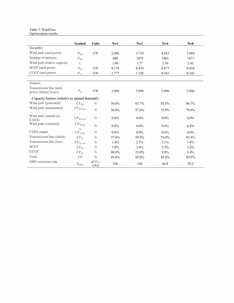
Table 3. Wind/Gas Optimization results.

Symbol Units N=1 N=2 N=4 N=8 Variables Wind park rated power PWP GW 2.096 3.719 4.825 5.084 Number of turbines NWT 608 1078 1401 1477 Wind park relative capacity rf 1.00 1.77 2.30 2.43 SCGT rated power PSC GW 0.174 0.474 0.677 0.654 CCGT rated power PCC GW 1.777 1.226 0.563 0.242 Outputs Transmission line rated power (before losses) PTL GW 2.096 2.096 2.096 2.096

Capacity factors (relative to annual demand): Wind park (generated) CFWP % 36.0% 63.7% 82.5% 86.7% Wind park (transmitted) CFWP,tran

s % 36.0% 57.6% 72.9% 79.9%

Wind park (stored via CAES) CFWP,stor % 0.0% 0.0% 0.0% 0.0%

Wind park (curtailed) CFWP,du

mp % 0.0% 6.0% 9.6% 6.8%

CAES output CFCAES % 0.0% 0.0% 0.0% 0.0% Transmission line (initial) CFTL % 37.4% 59.9% 76.0% 83.4% Transmission line (loss) CFTL,loss % 1.4% 2.3% 3.1% 3.4% SCGT CFSC % 1.0% 2.4% 2.3% 1.6% CCGT CFCC % 48.0% 25.0% 9.8% 3.4% Total CF % 85.0% 85.0% 85.0% 85.0% GHG emissions rate EGHG gCO2./

kWh 256 146 66.8 29.2

Table 4. Wind/CAES Optimization results.

Symbol Units N=1 N=2 N=4 N=8 Variables

Wind park rated power PWP GW 4.476 4.904 5.005 5.051 Number of turbines NWT 1298.297 1421.154 1453.552 1467.665

Wind park relative capacity rf 2.14 2.34 2.39 2.41 CAES compressor rated

power PC GW 2.380 1.280 0.802 0.419

CAES expander rated power PE GW 1.499 1.023 0.535 0.251 hS h 133.264 75.009 35.253 17.523

CAES storage duration (PTLhS) (GWh) 279.278 157.195 73.878 36.722

CAES expander rel. capacity rg 1.136 0.611 0.383 0.200 CAES compressor rel. cap. rc 0.716 0.488 0.255 0.120

Outputs

Transmission line rated power (before losses) PTL GW 2.096 2.096 2.096 2.096

Capacity factors (relative to annual demand): Wind park (generated) CFWP % 76.7% 83.4% 85.1% 85.9%

Wind park (transmitted) CFWP,tran

s % 51.9% 65.6% 74.2% 79.5%

Wind park (stored via CAES) CFWP,stor % 22.1% 12.9% 7.2% 3.7%

Wind park (curtailed) CFWP,du

mp % 2.7% 4.9% 3.8% 2.7%

CAES output CFCAES % 33.1% 19.4% 10.8% 5.5% Transmission line (initial) CFTL % 88.9% 88.8% 88.8% 88.8% Transmission line (loss) CFTL,loss % 3.9% 3.8% 3.8% 3.8%

Total CF % 85.0% 85.0% 85.0% 85.0%

GHG emissions rate EGHG gCO2./ kWh 108 63.5 35.4 18.0

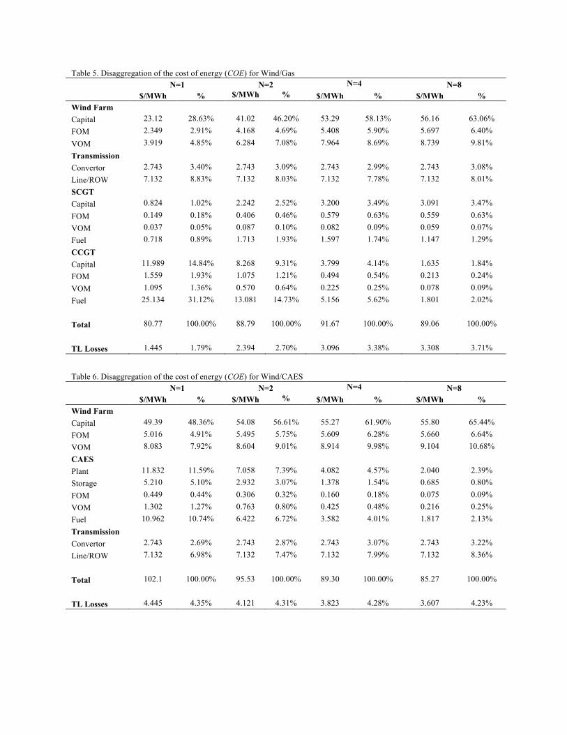
Table 5. Disaggregation of the cost of energy (COE) for Wind/Gas N=1 N=2 N=4 N=8 $/MWh % $/MWh % $/MWh % $/MWh % Wind Farm Capital 23.12 28.63% 41.02 46.20% 53.29 58.13% 56.16 63.06% FOM 2.349 2.91% 4.168 4.69% 5.408 5.90% 5.697 6.40% VOM 3.919 4.85% 6.284 7.08% 7.964 8.69% 8.739 9.81% Transmission Convertor 2.743 3.40% 2.743 3.09% 2.743 2.99% 2.743 3.08% Line/ROW 7.132 8.83% 7.132 8.03% 7.132 7.78% 7.132 8.01% SCGT Capital 0.824 1.02% 2.242 2.52% 3.200 3.49% 3.091 3.47% FOM 0.149 0.18% 0.406 0.46% 0.579 0.63% 0.559 0.63% VOM 0.037 0.05% 0.087 0.10% 0.082 0.09% 0.059 0.07% Fuel 0.718 0.89% 1.713 1.93% 1.597 1.74% 1.147 1.29% CCGT Capital 11.989 14.84% 8.268 9.31% 3.799 4.14% 1.635 1.84% FOM 1.559 1.93% 1.075 1.21% 0.494 0.54% 0.213 0.24% VOM 1.095 1.36% 0.570 0.64% 0.225 0.25% 0.078 0.09% Fuel 25.134 31.12% 13.081 14.73% 5.156 5.62% 1.801 2.02% Total 80.77 100.00% 88.79 100.00% 91.67 100.00% 89.06 100.00% TL Losses 1.445 1.79% 2.394 2.70% 3.096 3.38% 3.308 3.71%

Table 6. Disaggregation of the cost of energy (COE) for Wind/CAES N=1 N=2 N=4 N=8 $/MWh % $/MWh % $/MWh % $/MWh % Wind Farm Capital 49.39 48.36% 54.08 56.61% 55.27 61.90% 55.80 65.44% FOM 5.016 4.91% 5.495 5.75% 5.609 6.28% 5.660 6.64% VOM 8.083 7.92% 8.604 9.01% 8.914 9.98% 9.104 10.68% CAES Plant 11.832 11.59% 7.058 7.39% 4.082 4.57% 2.040 2.39% Storage 5.210 5.10% 2.932 3.07% 1.378 1.54% 0.685 0.80% FOM 0.449 0.44% 0.306 0.32% 0.160 0.18% 0.075 0.09% VOM 1.302 1.27% 0.763 0.80% 0.425 0.48% 0.216 0.25% Fuel 10.962 10.74% 6.422 6.72% 3.582 4.01% 1.817 2.13% Transmission Convertor 2.743 2.69% 2.743 2.87% 2.743 3.07% 2.743 3.22% Line/ROW 7.132 6.98% 7.132 7.47% 7.132 7.99% 7.132 8.36% Total 102.1 100.00% 95.53 100.00% 89.30 100.00% 85.27 100.00% TL Losses 4.445 4.35% 4.121 4.31% 3.823 4.28% 3.607 4.23%