IMM - Technical University of Denmark · iii Preface This thesis on the Scandina vian electricit...
182
IMM
Transcript of IMM - Technical University of Denmark · iii Preface This thesis on the Scandina vian electricit...

The Scandinavian
Electricity Power Market
and Market Power
Haukur Eggertsson
LYNGBY 2003
EKSAMENSPROJEKT
NR. 2003-46
IMM

Trykt af IMM, DTU

iii
Preface
This thesis on the Scandinavian electricity power market and market power,was written as part of my studies for a Master degree at the Department ofInformatics and Mathematical Modelling (IMM) in the Technical Univer-sity of Denmark (DTU), under the supervision of professor Henrik Madsen.
I wish to thank everyone who has supported me while working on thisthesis. Especially I would like to thank the following:
My supervisor, Henrik Madsen, for his e�orts in guiding me throughthe project and for his advice and encouragements.
The following for providing me with information and a better insight intothe subject:
Berith Bitsch Kristo�ersen and Bjarne Donslund at Eltra.Klaus Kaae Andersen and Henrik Aalborg Nielsen at IMM, DTU.Hilde Rosenblad at Nord Pool Spot.Jon Tøfting and Lars Kruse at Elsam.
The following for reviewing the manuscript, for their comments and im-provements on the text:
Anna Ellen DouglasEggert HaukssonÞorsteinn Yngvi Bjarnason
Lyngby, July, 2003
Haukur [email protected]

iv

v
Abstract
Recent high prices on the Scandinavian electric power market have led topublic scrutiny of the market and have been the source of investigation oflegal authorities.
Although the Nord Pool1 spot market is considered to be one of the mostsuccessful electricity markets in the world, and one of few internationalelectricity markets, the market is small in comparison to many other com-modity markets, and is as such, together with the di�culty of storing elec-tricity, less liquid and subject to more instability in prices and supply. Inaddition, due to limited transmission capacities between the areas thatform the common markets, prices often vary between market areas. Thiscan also give electricity generators a large market share in di�erent areas,even though they only hold a modest market share on the total market.
This thesis is a study of the possible uses of market power on the Nord Poolspot market and how this kind of market behavior, especially with regardto the game theory and Nash equilibria, can be detected.
This is certainly not by any means an accusation against any member of theNord Pool market, although the theoretical possibilities of some of themexercising market power, is discussed.
My �ndings are that searching for Nash equilibria is not the most e�ectiveway of market power detection, due to the many uncertainties involvedand the lack of information market power users as well as market powerdetectors will face.
1The Scandinavian power exchange

vi

vii
Contents
I Background 1
1 Introduction 3
1.1 Introduction . . . . . . . . . . . . . . . . . . . . . . . . . . . 3
1.2 Overview . . . . . . . . . . . . . . . . . . . . . . . . . . . . 4
2 The Scandinavian electricity market 7
2.1 Overview . . . . . . . . . . . . . . . . . . . . . . . . . . . . 7
2.2 The old structure . . . . . . . . . . . . . . . . . . . . . . . . 8
2.3 The shift to a market based structure . . . . . . . . . . . . 9
2.4 The creation of a pool . . . . . . . . . . . . . . . . . . . . . 10
2.5 Ownership and structure . . . . . . . . . . . . . . . . . . . . 10
2.6 Competition . . . . . . . . . . . . . . . . . . . . . . . . . . . 11
3 Nord Pool 13
3.1 The functions of Nord Pool . . . . . . . . . . . . . . . . . . 13
3.1.1 Elspot . . . . . . . . . . . . . . . . . . . . . . . . . . 13
3.1.2 Financial market . . . . . . . . . . . . . . . . . . . . 14
3.1.3 Elbas . . . . . . . . . . . . . . . . . . . . . . . . . . 15
3.2 The geographical markets . . . . . . . . . . . . . . . . . . . 15

viii CONTENTS
3.2.1 Eastern Denmark . . . . . . . . . . . . . . . . . . . . 15
3.2.2 Western Denmark . . . . . . . . . . . . . . . . . . . 15
3.2.3 Norway . . . . . . . . . . . . . . . . . . . . . . . . . 16
3.2.4 Sweden . . . . . . . . . . . . . . . . . . . . . . . . . 16
3.2.5 Finland . . . . . . . . . . . . . . . . . . . . . . . . . 16
3.2.6 Northern Germany . . . . . . . . . . . . . . . . . . . 16
4 Electricity 19
4.1 Characteristics of electricity . . . . . . . . . . . . . . . . . . 19
4.2 Sources of power . . . . . . . . . . . . . . . . . . . . . . . . 20
4.2.1 Hydropower . . . . . . . . . . . . . . . . . . . . . . . 20
4.2.2 Nuclear power . . . . . . . . . . . . . . . . . . . . . 21
4.2.3 Coal and oil . . . . . . . . . . . . . . . . . . . . . . . 21
4.2.4 Gas . . . . . . . . . . . . . . . . . . . . . . . . . . . 22
4.2.5 Wind power . . . . . . . . . . . . . . . . . . . . . . . 22
4.2.6 Other sources . . . . . . . . . . . . . . . . . . . . . . 23
II Theory 25
5 Market power 27
5.1 Competition, monopoly and oligopoly . . . . . . . . . . . . 27
5.2 Detection of market power . . . . . . . . . . . . . . . . . . . 30
6 Competition 33
6.1 Perfect competition . . . . . . . . . . . . . . . . . . . . . . . 33
6.2 Monopoly . . . . . . . . . . . . . . . . . . . . . . . . . . . . 33
6.3 Oligopoly . . . . . . . . . . . . . . . . . . . . . . . . . . . . 34

CONTENTS ix
7 Game theory 37
7.1 De�nition . . . . . . . . . . . . . . . . . . . . . . . . . . . . 37
7.2 Games and market behavior . . . . . . . . . . . . . . . . . . 38
7.3 Mixed strategy . . . . . . . . . . . . . . . . . . . . . . . . . 41
7.4 Reputation and threats . . . . . . . . . . . . . . . . . . . . 41
III Study 43
8 Data and machines 45
8.1 The data from Eltra . . . . . . . . . . . . . . . . . . . . . . 45
8.1.1 Supply and demand . . . . . . . . . . . . . . . . . . 45
8.1.2 Other data from Eltra . . . . . . . . . . . . . . . . . 47
8.2 Nord Pool . . . . . . . . . . . . . . . . . . . . . . . . . . . . 47
8.3 Sun�re . . . . . . . . . . . . . . . . . . . . . . . . . . . . . . 47
9 Characteristics of the Scandinavian electricity market 49
9.1 Overview . . . . . . . . . . . . . . . . . . . . . . . . . . . . 49
9.2 Competition and cooperation . . . . . . . . . . . . . . . . . 52
9.3 Demand . . . . . . . . . . . . . . . . . . . . . . . . . . . . . 52
10 Market power on Nord Pool's spot market 57
10.1 Who could be using market power? . . . . . . . . . . . . . . 57
10.2 Big producers . . . . . . . . . . . . . . . . . . . . . . . . . . 58
10.2.1 ENERGI E2 . . . . . . . . . . . . . . . . . . . . . . 58
10.2.2 Elkraft . . . . . . . . . . . . . . . . . . . . . . . . . . 59
10.2.3 Elsam . . . . . . . . . . . . . . . . . . . . . . . . . . 59
10.2.4 Eltra . . . . . . . . . . . . . . . . . . . . . . . . . . . 59
10.2.5 Statkraft . . . . . . . . . . . . . . . . . . . . . . . . 60

x CONTENTS
10.2.6 Vattenfall . . . . . . . . . . . . . . . . . . . . . . . . 60
10.2.7 Sydkraft . . . . . . . . . . . . . . . . . . . . . . . . . 61
10.2.8 Fortum . . . . . . . . . . . . . . . . . . . . . . . . . 61
10.2.9 E.On . . . . . . . . . . . . . . . . . . . . . . . . . . . 61
10.3 Winners and losers . . . . . . . . . . . . . . . . . . . . . . . 62
10.4 The rules of the game . . . . . . . . . . . . . . . . . . . . . 62
10.5 As time goes by . . . . . . . . . . . . . . . . . . . . . . . . . 63
10.6 How can market power be exercised? . . . . . . . . . . . . . 63
10.6.1 Raising prices . . . . . . . . . . . . . . . . . . . . . . 64
10.6.2 Withholding production . . . . . . . . . . . . . . . . 74
10.6.3 Wrong predictions . . . . . . . . . . . . . . . . . . . 81
10.6.4 Blocking grid lines . . . . . . . . . . . . . . . . . . . 82
10.6.5 Cooperation . . . . . . . . . . . . . . . . . . . . . . . 84
10.6.6 Leaving the spot market . . . . . . . . . . . . . . . . 85
10.7 Detecting market power . . . . . . . . . . . . . . . . . . . . 86
10.7.1 By whom? . . . . . . . . . . . . . . . . . . . . . . . . 86
10.7.2 And how? . . . . . . . . . . . . . . . . . . . . . . . . 86
11 Price strategies 89
11.1 Overview . . . . . . . . . . . . . . . . . . . . . . . . . . . . 89
11.2 Export and import . . . . . . . . . . . . . . . . . . . . . . . 90
11.3 Selecting a strategy . . . . . . . . . . . . . . . . . . . . . . . 91
11.3.1 Highest accepted bid . . . . . . . . . . . . . . . . . . 91
11.3.2 Fully and partially accepted bids . . . . . . . . . . . 92
11.3.3 Second highest accepted bid . . . . . . . . . . . . . . 93
11.3.4 Lowest unaccepted bid . . . . . . . . . . . . . . . . . 93
11.3.5 Power players . . . . . . . . . . . . . . . . . . . . . . 95

CONTENTS xi
IV Calculations 97
12 Price calculation algorithms 99
12.1 The price of everything . . . . . . . . . . . . . . . . . . . . 99
12.1.1 Eltra's method . . . . . . . . . . . . . . . . . . . . . 99
12.1.2 IMM's veri�cation algorithm . . . . . . . . . . . . . 102
12.1.3 Revision . . . . . . . . . . . . . . . . . . . . . . . . . 102
12.2 Transmission between markets . . . . . . . . . . . . . . . . 103
12.3 Preparing the data . . . . . . . . . . . . . . . . . . . . . . . 104
13 Search algorithms 107
13.1 Nash equilibria . . . . . . . . . . . . . . . . . . . . . . . . . 107
13.1.1 All solutions . . . . . . . . . . . . . . . . . . . . . . 108
13.1.2 Iterative search for Nash equilibria . . . . . . . . . . 109
13.1.3 Hourly Nash equilibria . . . . . . . . . . . . . . . . . 110
13.2 Pareto optimality . . . . . . . . . . . . . . . . . . . . . . . . 116
13.3 Simulating annealing . . . . . . . . . . . . . . . . . . . . . . 118
13.3.1 Application of simulated annealing to �nd Nash equi-libria . . . . . . . . . . . . . . . . . . . . . . . . . . . 120
13.3.2 Application of simulated annealing to �nd Pareto op-timality . . . . . . . . . . . . . . . . . . . . . . . . . 121
13.4 Longer periods . . . . . . . . . . . . . . . . . . . . . . . . . 121
13.4.1 Cycles . . . . . . . . . . . . . . . . . . . . . . . . . . 121
13.4.2 Weeks . . . . . . . . . . . . . . . . . . . . . . . . . . 122
13.4.3 Nash and Pareto . . . . . . . . . . . . . . . . . . . . 122
13.5 Comparison to actual prices . . . . . . . . . . . . . . . . . . 125
13.6 Searches and results . . . . . . . . . . . . . . . . . . . . . . 130
13.6.1 To be or not to be . . . . . . . . . . . . . . . . . . . 130

xii CONTENTS
13.6.2 Incomplete information . . . . . . . . . . . . . . . . 130
13.6.3 Unpredictability . . . . . . . . . . . . . . . . . . . . 131
13.6.4 Enlightenment . . . . . . . . . . . . . . . . . . . . . 131
13.6.5 Market power and Nash equilibria . . . . . . . . . . 132
V Conclusions 133
14 Conclusions 135
14.1 Overview . . . . . . . . . . . . . . . . . . . . . . . . . . . . 135
14.2 Results . . . . . . . . . . . . . . . . . . . . . . . . . . . . . . 136
14.2.1 Market power . . . . . . . . . . . . . . . . . . . . . . 136
14.2.2 Nash equilibrium . . . . . . . . . . . . . . . . . . . . 136
14.2.3 Pareto optimality . . . . . . . . . . . . . . . . . . . . 136
14.2.4 Parameters . . . . . . . . . . . . . . . . . . . . . . . 136
14.2.5 Incomplete information . . . . . . . . . . . . . . . . 137
14.3 Conclusions . . . . . . . . . . . . . . . . . . . . . . . . . . . 137
14.4 Further studies . . . . . . . . . . . . . . . . . . . . . . . . . 137
VI Appendices 139
A Elspot areas and bidding information 141
A.1 ELSPOT AREAS AND BIDDING INFORMATION . . . . 141
A.2 BIDDING FOR PURCHASE AND SALE . . . . . . . . . . 142
A.3 PRICE SETTING . . . . . . . . . . . . . . . . . . . . . . . 143
A.4 REPORTS OF PURCHASE AND SALE . . . . . . . . . . 144

CONTENTS xiii
B Matlab codes 147
B.1 Price calculations . . . . . . . . . . . . . . . . . . . . . . . . 147
B.2 Data preperation . . . . . . . . . . . . . . . . . . . . . . . . 153
B.3 Iterative search for Nash equilibrium . . . . . . . . . . . . . 156
Bibliography 161

xiv CONTENTS

xv
List of Figures
4.1 Daily wind power in western Denmark in 2002 . . . . . . . 23
4.2 Wind power per hour from December 1st to 7th 2002 in west-ern Denmark . . . . . . . . . . . . . . . . . . . . . . . . . . 24
5.1 Use of market power . . . . . . . . . . . . . . . . . . . . . . 28
5.2 Assuming bids from competitors . . . . . . . . . . . . . . . 29
9.1 Hourly consumption in Sweden May 15th to May 21st 2003 50
9.2 Maximum possible export from each area . . . . . . . . . . 51
9.3 Total hourly income from sales in Sweden . . . . . . . . . . 54
9.4 Demand in Finland . . . . . . . . . . . . . . . . . . . . . . . 54
10.1 Tuesday: Changes in Elsam's pro�t with di�erent markups 65
10.2 Tuesday: Changes in Vattenfall's pro�t with di�erent markups 66
10.3 Tuesday: Prices when Vattenfall changes its markup . . . . 66
10.4 Tuesday: Changes in Sydkraft's pro�t with di�erent markups 67
10.5 Tuesday: Prices when Sydkraft changes its markup . . . . . 67
10.6 Tuesday: Changes in Fortum's pro�t with di�erent markups 68
10.7 Tuesday: Changes in E.On's pro�t with di�erent markups . 68
10.8 Tuesday: Prices when E.On changes its markup . . . . . . . 69

xvi LIST OF FIGURES
10.9 Monday: Changes in E2's pro�t with di�erent markups . . 70
10.10Monday: Prices when E2 changes its markup . . . . . . . . 70
10.11Monday: Changes in Elsam's pro�t with di�erent markups 71
10.12Monday: Prices when Elsam changes its markup . . . . . . 71
10.13Monday: Changes in Statkraft's pro�t with di�erent markups 72
10.14Monday: Prices when Statkraft changes its markup . . . . . 72
10.15Monday: Changes in Vattenfall's pro�t with di�erent markups 73
10.16Monday: Changes in Sydkraft's pro�t with di�erent markups 73
10.17Monday: Changes in Fortum's pro�t with di�erent markups 74
10.18Tuesday: Hourly change in E2's pro�t when production iswithheld . . . . . . . . . . . . . . . . . . . . . . . . . . . . . 76
10.19Tuesday: Hourly change in Elsam's pro�t when productionis withheld . . . . . . . . . . . . . . . . . . . . . . . . . . . 76
10.20Tuesday: Hourly change in Statkraft's pro�t when produc-tion is withheld . . . . . . . . . . . . . . . . . . . . . . . . . 77
10.21Tuesday: Hourly change in Vattenfall's pro�t when produc-tion is withheld . . . . . . . . . . . . . . . . . . . . . . . . . 77
10.22Tuesday: Hourly change in Sydkraft's pro�t when produc-tion is withheld . . . . . . . . . . . . . . . . . . . . . . . . . 78
10.23Tuesday: Hourly change in Fortum's pro�t when productionis withheld . . . . . . . . . . . . . . . . . . . . . . . . . . . 78
10.24Tuesday: Hourly change in E.On's pro�t when productionis withheld . . . . . . . . . . . . . . . . . . . . . . . . . . . 79
10.25Monday: Hourly change in pro�t when production is withheld 80
10.26Monday: A closer look at pro�t . . . . . . . . . . . . . . . . 80
10.27Optimal wind power production for Elsam . . . . . . . . . . 81
10.28Turning o� eastern Denmark . . . . . . . . . . . . . . . . . 83
10.29A closer look at the Sound connection . . . . . . . . . . . . 83
10.30Prices when holding up the line . . . . . . . . . . . . . . . . 84

LIST OF FIGURES xvii
10.31Optimal wind power production . . . . . . . . . . . . . . . . 85
11.1 E�ects of export/import on prices in Norway and Sweden . 91
11.2 Supply and demand on the Finnish market . . . . . . . . . 92
11.3 Demand and supply in western Denmark . . . . . . . . . . . 93
11.4 Gains and losses for the holder of the lowest unaccepted bid 94
12.1 Sydkraft and supply in Sweden . . . . . . . . . . . . . . . . 105
13.1 The rough reality of pro�t . . . . . . . . . . . . . . . . . . . 111
13.2 Batman's head? . . . . . . . . . . . . . . . . . . . . . . . . . 111
13.3 Suggested markup of production cost . . . . . . . . . . . . . 112
13.4 Pro�t of each player . . . . . . . . . . . . . . . . . . . . . . 112
13.5 Prices on each market . . . . . . . . . . . . . . . . . . . . . 113
13.6 The never ending story . . . . . . . . . . . . . . . . . . . . . 113
13.7 The Finnish gambit . . . . . . . . . . . . . . . . . . . . . . 114
13.8 Mountain of money? . . . . . . . . . . . . . . . . . . . . . . 115
13.9 The �nal price to pay for the competition . . . . . . . . . . 115
13.10Iterated markup on Tuesday . . . . . . . . . . . . . . . . . . 116
13.11Pareto on Tuesday . . . . . . . . . . . . . . . . . . . . . . . 118
13.12A new Finnish gambit . . . . . . . . . . . . . . . . . . . . . 119
13.13All is lost . . . . . . . . . . . . . . . . . . . . . . . . . . . . 119
13.14Whole week Nash equilibrium from 0 markup . . . . . . . . 123
13.15Pro�t change for weekly Nash equilibrium search . . . . . . 124
13.16Whole week Nash equilibrium from 10% markup . . . . . . 124
13.17Dwindling pro�t . . . . . . . . . . . . . . . . . . . . . . . . 125
13.18The merit of cooperation . . . . . . . . . . . . . . . . . . . . 126
13.19Prices in western Denmark . . . . . . . . . . . . . . . . . . 127

xviii LIST OF FIGURES
13.20Prices in Sweden . . . . . . . . . . . . . . . . . . . . . . . . 127
13.21Prices in Germany . . . . . . . . . . . . . . . . . . . . . . . 128
13.22Average daily system price on the Nord Pool spot market . 129

Part I
Background
1


3
Chapter 1
Introduction
1.1 Introduction
The main motivation behind this thesis is based on the concern that marketpower is possibly being used on the Scandinavian electricity market, NordPool, i.e. on the spot market, and on how such a suspicion can be reinforcedby analysis.
Eltra, the transmission system operator in western Denmark, see section10.2.4, has worked with IMM (the Department of Informatics and Math-ematical Modelling at the Technical University of Denmark (DTU)), on anumber of di�erent projects concerning electricity, such as wind power andthe electricity market in general. Eltra has shown interest in the possibleuse of market power on the Nord Pool spot market, and has suggestedstudies on the matter with special reference to the game theory and Nashequilibria, at IMM. To follow up, Eltra has provided data and other usefulinformation, on which this thesis has mainly been based on.
The recent high prices on the Scandinavian electric power market have beenthe source of speculations whether market power is being used and whetherthe deregulation of the Scandinavian electricity power market is justi�ed.
Both Nord Pool and transmission system operators have an interest inreinforcing the credibility of the market and are consequently interested indetecting unusual market behavior.

4 Chapter 1. Introduction
The Nord Pool market area consists of Denmark, Norway, Sweden andFinland, each with di�erent sources of energy, demand and production be-havior. The limited transmission capacity of electricity between the mar-kets creates an interesting situation where, under certain circumstances,producers, with a small market share on the overall market, will �nd them-selves holding a large market share in their own market when congestionoccurs. As large market share is one of the key factors for market powerto be pro�table, these temporary semimonopoly situations may o�er sometempting opportunities for certain producers.
1.2 Overview
In Chapter 2, The Scandinavian electricity market, I describe the estab-lishment of the common Scandinavian electricity market.
In Chapter 3, Nord Pool, I discuss and describe the functions of Nord Pool,especially its spot market and the geographical markets on which NordPool operates.
In Chapter 4, Electricity, I discuss the characteristics of electricity, its dis-tinction from other commodities as regards storing and transmitting, andthe di�erent sources of electricity.
In Chapter 5, Market power, I de�ne market power and the necessary in-formation that must be available for its detection.
In Chapter 6, Competition, I discuss the di�erent forms of competition, andtheir theoretical background.
In Chapter 7, Game theory, I introduce the element of the game theory Iwill use in this thesis as well as de�ning certain concepts.
In Chapter 8, Data and Machines, I discuss the data and the computersused for calculations in this thesis.
In Chapter 9, Characteristics of the Scandinavian electricity market, I dis-cuss precisely that.
In Chapter 10, Market power on Nord Pool's spot market, I introduce thepossible market power users, discuss di�erent forms of market power and�nally how market power may be detected.

1.2 Overview 5
In Chapter 11, Price strategies, I discuss how individual electricity produc-ers should choose their price strategies in order to optimize their pro�t.
In Chapter 12, Price calculation algorithms, I discuss some various methodsfor calculating prices on the Nord Pool spot market.
In Chapter 13, Search algorithms, I introduce some methods for the searchof Nash equilibria and Pareto optimal solutions for short and long periodsof time. I will also compare the �ndings to the actual prices of time as wellas discussing the value of the �ndings for the detection of market power.
In Chapter 14, Conclusions, I draw my �nal conclusions.

6 Chapter 1. Introduction
7
Chapter 2
The Scandinavian electricity
market
2.1 Overview
The Scandinavian countries have traded electrical power for decades andthus have one of the world's most developed international power market.In the last decade, the trading system has changed dramatically, movingfrom the old model of cooperation among the leading vertically integratedutilities in each country, under the Nordel agreement, to competitive marketrules. (Nord Pool).
The di�erences in the mixture of power generation largely explain theestablishment of interconnections in Scandinavia. Norway relies entirelyon hydropower, while Denmark generates most of its power in thermalplants, mainly from imported coal and, lately, increasingly from windpower. Power generation in Sweden is a mixture of about half hydro andhalf nuclear generation, and in Finland it is mixture of hydro (25 %), con-ventional thermal (45 %), and nuclear (30 %) plants. The di�erences in thepower generation structure have made it economically attractive to tradepower, allowing the countries to optimize production.
These countries also have strong cultural and economic ties, even thoughNorway is currently outside the European Union (EU). However, as a mem-

8 Chapter 2. The Scandinavian electricity market
ber of European Free Trade Association (EFTA), Norway is also a memberof the European Economic Area (EEA), which in a way intergrades someof the EFTA countries, i.e. Norway, Iceland and Liechtenstein into the EU,applying large bits of EU legislation to the area with the aim to make tradebetween the EEA members as easy as between members of the EU.[1]
2.2 The old structure
Before the move to the international pool, the power sectors of Norway,Sweden and Finland all had an oligopoly structure, with dominant stateowned enterprizes that also controlled the national grids, even though therewere di�erences in structure, ownership, and regulation.
Norway's power sector was dominated by the government owned integratedutility Statkraft, which also operated the national grid. There were alsomany small local and regional utilities. Between �fty and sixty companies,many owned by local or regional authorities, were involved in the transmis-sion of electricity at the regional level. The local and regional utilities hadgained access to the national grid in 1969 and could buy and sell powerthrough a spot market. Electricity was distributed locally by around 200companies, many of which were owned by municipalities.
In Sweden, about half the generation was government owned through Vatten-fall, which also operated the national grid and provided distribution servicesin parts of the country. About ten other integrated utilities of various sizesalso used the national grid, but a relatively high network fee made it un-economic for smaller utilities to use it. Like Norway, Sweden had a largenumber of distribution companies, many owned by municipalities.
In Finland the state owned Imatran Voima Oy (IVO) was the largest util-ity. IVO also operated the national grid. However, much of the powergeneration was owned by Finnish industries, which formed a transmissioncompany, TVS, to interconnect their generation and supply areas.
In Denmark, for geographical reasons, the grid is divided into two mainparts: Jutland and Funen (western Denmark) and the islands east of theGreat Belt (eastern Denmark). In each of these two areas the generationand distribution utilities, mostly owned by municipalities, formed specialpurpose organizations to manage the extra high-voltage grids and the co-ordinated operation.
2.3 The shift to a market based structure 9
Trading of electricity between the countries was enabled through Nordel,an organization set up in the 1960s to promote cooperation among thelargest electricity producers in each country. Nordel was based on theprinciple that each country would build enough generating capacity to beself-su�cient. Trading was meant to achieve optimal dispatch of a largersystem, and investment in interconnection was generally based, not on netexports, but on expected savings from pooling available generating capacity.The countries exchanged information on their marginal cost of production.When there was a di�erence, trading took place at a price that was theaverage of the two marginal costs.
The cost-plus structure in the Nordic power sector led to over investmentand poor return on equity. But because the system retained a degree ofcompetition, there were no signi�cant operating e�ciency problems in theutilities.[1]
2.3 The shift to a market based structure
The shift to an international pool was triggered by power sector reformsin Norway starting in the early 1990s. Norway introduced competition inelectricity supply in 1991 through reforms aimed at reducing regional dif-ferences in the cost of power, promoting operational e�ciency in generationand distribution, and achieving more e�cient development of the power sec-tor. Statkraft's transmission activities were spun o� to a new national gridcompany, Statnett SF. In addition, all transmission networks were openedto third-party access, and vertically integrated companies had to adoptseparate accounting for generation, distribution, and supply activities.
In Sweden, reform was fuelled by discontent among the private power com-panies stemming from Vattenfall's control of the national grid, and dissat-isfaction among the smaller power companies and among customers overtheir lack of access to the market for occasional power. The �rst major step,taken in 1991, was to corporatize Vattenfall's generation and distributionactivities. However, Vattenfall remains government owned. The nationalgrid was retained as a government owned institution, Svenska Kraftnät,which also serves as the system operator. The networks were graduallyopened to new players, and a new electricity act allowing a competitivemarket �nally took e�ect in January 1996.

10 Chapter 2. The Scandinavian electricity market
Finland introduced a new energy legislation in 1995. IVO had already orga-nized its grid activity into a separate company, IVS. But with the privatelyowned grid company TVS, Finland had two overlapping grid companies forseveral years. Since September 1997, Finland has had a single, merged gridcompany, Fingrid, which also acts as the system operator.
Reform moved more slowly in Denmark because of the power sector's dif-ferent structure, with two unconnected groups owned by municipalities orcooperatives, each with a monopoly in its area. A new legislation was in-troduced in 1996, opening the grids to negotiated third-party access andallowing competition for large consumers, distributors and generators.[1]
2.4 The creation of a pool
Norway led the way in reform, by opening up a spot market in 1992. Asimilar power market in Sweden would have been problematic to manage,as Vattenfall and Sydkraft, the two largest generating companies, togethercontrol about 75 % of generating capacity. However, the Norwegian marketalso experienced problems. Because almost all the power in Norway isproduced by hydroelectric plants, the spot market price was very volatile.A combined Norwegian-Swedishmarket would address the problems of bothcountries. A decision was therefore made to establish a joint electricitytrading exchange in January 1996, the design being based on the Norwegianexperience. The grid operators own the company, Nord Pool, that organizesthe market. Finland joined the power exchange in June 1998. western andeastern Denmark joined in July 1999 and October 2000 respectively.[1]
2.5 Ownership and structure
Setting up the pool did not require privatizing government owned compa-nies. A mixture of companies continues to operate in the Nordic powersectors, from large government owned utilities to privately and municipallyowned companies of various sizes, running generation, regional networksand distribution systems, and supplying power to consumers. But owner-ship of the international interconnections that existed in the Nordel area,when the sectors were restructured in Finland, Norway and Sweden, hasbeen transferred to the grid company in each country. This has opened

2.6 Competition 11
trading to all the players in the wholesale markets; generators, distribu-tors, and large consumers.
Competitive pressures in the electricity market have resulted in severalchanges in ownership and structure in the sector, including some cross-ownerships between countries and the entry of some foreign power com-panies. In addition to the traditional power companies, other players cantrade on the market, including brokers, oil companies, foreign power com-panies and power trading companies representing consumer groups.[1]
2.6 Competition
Strict regulation of the electrical network service ensures that third-partyaccess works. However, it is generally assumed that the market is able totake care of itself under the supervision of national competition authorities.
With increasing privatization of the electricity generation, the forming ofthe Scandinavian electricity market was also intended to reduce the risk ofmonopolistic behavior and the use of market power, while the bene�ts offree enterprize would be enjoyed.
However, around Easter 2002 prices rose and the di�erence between elec-tricity sold and electricity o�ered on the market became so great that aninvestigation was launched, reaching all the Scandinavian electricity pro-ducers. Therefore, the use of market power is considered to be a realpossibility.[2]

12 Chapter 2. The Scandinavian electricity market

13
Chapter 3
Nord Pool
3.1 The functions of Nord Pool
Nord Pool operates three markets, each with a di�erent purpose. In thisthesis, however, the main focus will be on the spot market, Elspot. Theother two are the Financial market and Elbas.
3.1.1 Elspot
The spot market for electrical power, organized by Nord Pool, trades inhourly contracts for the following day. It is open to all parties that havesigned the necessary agreements with Nord Pool. Bids are submitted eachmorning, and supply and demand curves are then constructed to providethe price (the system price) and the traded quantity for each hour dur-ing the next day. The price of the power to balance the system is alsodetermined through bidding. Elkraft, Eltra, Statnett, Svenska Kraftnät,and Fingrid are each responsible for balancing the system in their areas.When di�erences in prices prevail between areas, these companies tari� theelectricity until balance is obtained with full use of the international trans-mission lines. These tari�s can be vast if the price gap between countriesis great.
Example 3.1 If the market price in Norway is x and the market price inSweden is y, y > x and the power which can be delivered from Norway to

14 Chapter 3. Nord Pool
Sweden is z, the transmission system operators in Norway and Sweden willsplit the pro�t of (y − x) × z
The Elspot market is a day-ahead physical-delivery power market and thedeadline for submitting bids for all delivery hours of the the following dayis 12 am (noon). The products traded on the Elspot Market are bids ofa one-hour duration, block bids and �exible hourly bids.
Contracts on the Elspot market are one hour physical power (delivery toor take-o� from the grid) obligations; minimum contract size is 0,1MWh/h.
Hourly Bid is a sequence of price/volume pairs for each speci�ed hour.Volumes are stated in MWh. In bidding, purchases are designated aspositive numbers and sales as negative numbers.
Block Bid is an aggregated bid for several consecutive hours with a �xedbidding price and volume. The block bid price is compared with theaverage hourly price within the block period. A block bid must beaccepted in its entirety and if it is accepted the contract covers allhours and the volume speci�ed in the bid.
Flexible Hourly Bid is a sales bid for a single hour with a �xed priceand volume. The hour is not speci�ed, but instead the bid will beaccepted in the hour with the highest price, given that the price ishigher than the limit set in the bid.
The trade on the spot market amounted to 124 TWh in 2002 or 32% of thetotal electricity consumption in Scandinavia for that year, and rose from29% from 2001.[4]
Further information about Elspot areas and bidding information can befound in appendix A.
3.1.2 Financial market
In addition to the spot market, Nord Pool o�ers futures contracts, whichare traded as weekly contracts four to seven weeks ahead, as blocks of fourweeks up to 52 weeks ahead, or as seasons up to three years ahead. Thefutures are purely �nancial contracts used for price hedging. The bulk ofthe volume traded is in standardized �nancial contracts, often referred toas over-the-counter (OTC) contracts. The liquidity of the OTC market isquite high, particularly for the nearest season. Contracts can be resold, ora position netted out by making an opposite contract.

3.2 The geographical markets 15
In addition to the spot and futures markets there is direct trading betweenparties in bilateral forwards. These bilateral contracts normally involvephysical deliveries and are often tailor-made to particular requirements.Despite the diversity in trading instruments, most of the trading betweenplayers still takes place under bilateral contracts for physical delivery whichwere signed before the reform.[5]
3.1.3 Elbas
The Elbas Market is a physical market for power trading in hourly contractsfor delivery on the same or next day. It enables trading around the clockevery day of the year, covering individual hours up to one hour beforedelivery. One function is to be the adjustment market to the Elspot Market.The participants are mainly power producers, distributors, and industriesand brokers in Finland and Sweden.[6]
3.2 The geographical markets
The Nord Pool market is composed of �ve market areas with several limita-tions of electricity transmission between them. These areas are: Denmark,which is divided into two areas by the Great Belt, Norway, Sweden andFinland.
3.2.1 Eastern Denmark
Eastern Denmark (DKE) consists of all the Danish islands east of the GreatBelt, with the exception of Bornholm. It has connections to Sweden andGermany, but not to western Denmark. Eastern Denmark depends heavilyon coal and wind power for electricity generation.
3.2.2 Western Denmark
Western Denmark (DKW) consists of Jutland, Funen and other smallerislands west of the Great Belt. Western Denmark has connections to Nor-way, Sweden and Germany. It depends primarily on coal and wind powerfor electricity generation.[7]

16 Chapter 3. Nord Pool
3.2.3 Norway
Norway (NOR) has connections to western Denmark, Sweden and a smallone to Finland. Norway has also connections to Russia. For electricitygeneration, Norway depends mostly on hydropower. Due to internal trans-mission limitations of the Norwegian power grid system, tari�s are used onthe congested points. Therefore there can be di�erent prices in di�erentareas of Norway.[7]
3.2.4 Sweden
Sweden (SWE) has connections to all the other markets of Nord Pool aswell as to Poland. The Swedish electricity market depends mainly on hy-dropower, nuclear power and other thermal power as coal and gas plants.When congestion occurs in the Swedish local grid transmission system,Svenska Kraftnät buys more expensive power from areas where the mar-ket price causes power shortage; i.e. buy enough of power from inside thearea to satisfy demand, at price above the market price. The extra costcaused by this intervention is covered by �xed charges on the users of thetransmission system.[7]
3.2.5 Finland
Finland (FIN) has connections to Norway and Sweden on the Nord Pool aswell as to Russia. Finland depends mostly on coal, nuclear and hydropowerfor electricity generation.[7]
3.2.6 Northern Germany
Although northern Germany (NGE) is not part of the Scandinavian Powermarket, it is currently the only area which is expected to have similar pricesas in Scandinavia. Unlike Russia and Poland which also have connectionsto Finland and Sweden respectively, the import from these countries isusually �xed as the maximum import possible due to international trans-mission restrictions. However, the similarities between the Scandinavianand German prices make the German market more interactive. In this the-sis, the German market is therefore sometimes considered a special market

3.2 The geographical markets 17
area, although strictly speaking it is not. The data used for most calcu-lations assume power plants and production in northern Germany whichmay interact with the other markets. northern Germany has connectionsto both Danish markets as well as to Sweden. The northern Germany'spower supply comes mainly from nuclear, coal and wind sources.[7]

18 Chapter 3. Nord Pool

19
Chapter 4
Electricity
4.1 Characteristics of electricity
Since its �rst practical application in the 19th Century, electricity has be-come one of the most essential elements of modern society. Without it mostservices would cease to operate and, in the western world, electricity hasbeen taken for granted for almost a century.
The characteristics of electricity vary from many other products. As withmost commodities, prices will, in the long term, re�ect the production costof the last unit sold. If not producers will either drop out of the market ornew ones enter. However, electricity di�ers from most other commoditiesin three ways.
1. Lack of storage ability. There is no economically viable storage ofelectricity and though it can be stored in all kinds of batteries, e.g. hy-drogen cells, storing large quantities is both expensive and ine�cient.Therefore, the same volume of electricity used must be produced eachtime, and while the consumption of electricity varies during the dayand between seasons, so must the production. Hence, there is neverany stock in reserve, nor can low consumption periods be used toprepare for high peak consumption periods. This makes the price ofpower vary considerably during the hours of the day, and betweenseasons, as temperature is one of the key consumption variables.

20 Chapter 4. Electricity
2. Transmission. Transporting electricity is subject to other law thanmost commodities. If the necessary grid lines are available, electricitycan be transmitted in a very short time over long distances, eventhough this may a�ect its quality. However, these grid lines havea limited transmission capacity and are often not available. Thus,electricity needs its own kind of infrastructure for transmission asopposed to most other commodities.
3. Inelastic demand. Studies indicate that electricity demand is usuallyrelatively inelastic and will respond only slowly to consistent pricepressure. Most customers still pay �xed prices based on rate schedulesset by regulators. Short time demand curves are almost vertical.
4.2 Sources of power
The main sources of power for electricity generation in Scandinavia are:
• Hydropower• Nuclear power• Coal and oil• Gas• Wind power
In the following section the characteristics of these di�erent sources will bediscussed brie�y.
4.2.1 Hydropower
Hydropower is the main source of energy in Norway and, to a lesser extent,in Sweden and Finland. There are two kinds of hydropower plants, dammedsites and free-�owing sites. Dams are often expensive to build, but cheapto maintain and operate. Although fuel cost is essentially zero while thewater lasts, and there is no emission of waste into the environment, thedams themselves, often with a huge man-made reservoir lake and thussinking of land, have been the source of increased environmental concern.The potential of harnessing more hydropower in Scandinavia is consideredalmost exhausted.
Free-�ow hydropower plants are not very �exible, even though they tend toproduce more during the day than the night, but then again more during

4.2 Sources of power 21
the summer than the winter when the need for energy is greater. Plantsusing water reservoirs are far more �exible and can store water duringlow demand periods, but there is of course a limit to how much they canproduce during peak demand. There is also the uncertainty of how muchwater will �ow into the reservoir during coming seasons, which means thatthe operators of such dams will want to save the reservoir for times withhigh power prices and thus limit the availability of cheap power. Therefore,it is quite di�cult to estimate the �production cost� of reservoir hydropowerplants. It can therefore be in the interest of consumers that hydropowerplants do not o�er their prices at too low levels as it may cause the reservoirsto empty before spring and thus generate very high prices, from which thehydropower owners will not bene�t, having spent all their water earlier. Asfree-�ow hydropower plants can be treated much like windmills, only morepredictably, the power will be sold at any price, i.e. minimum price or zeroat the auction.[8]
4.2.2 Nuclear power
The only nuclear power plants in Scandinavia are to be found in Swedenand Finland. Although fuel cost for nuclear plants is lower than for coalor gas plants, maintenance and security cost is higher, and building theseplants is more expensive and more time consuming. Nuclear power plantsemit virtually no airborne pollutants, and overall far less waste materialthan fossil fuel based power plants. However, this relatively small amountof waste, which is in the form of highly radioactive spent fuel and needsto be handled with great care and forethought due to the long half-lives ofthe waste, has been of environmental concern. There is also the securityrisk, often connected with accidents at Three Mile Island and Chernobyl,but also in case of terrorism and war, which theoretically could end in adisaster. Nuclear power plants are also quite in�exible in production andit takes long time to either increase or decrease the production, i.e. theydo not handle peaks very well.[9]
4.2.3 Coal and oil
The burning of coal and oil to generate energy and hot water, is the mainpower source in Denmark and Finland, and to a lesser extent in Swedenand Germany. The bene�ts of coal and oil power plants are that they
22 Chapter 4. Electricity
are rather cheap to build and operate, but the fuel cost is higher than fornuclear plants although lower than for gas plants. They can also, as aside product, be used to heat water for commercial use such as domesticheating, especially during the winter. This means that the operation of coalplants is more pro�table during the winter when demand for both electricityand hot water is normally higher. As coal plants are often required toproduce hot water, power will be sold at any price. However, the emissionproblem with fossil fuel goes beyond greenhouse gases and includes acidgases (sulfur dioxide and nitrogen oxides, which is also a greenhouse gas),particulates, heavy metals (notably mercury, but also including radioactivematerials) and solid waste such as ash. Due to the above and internationalenvironmental agreements such as the Kyoto Protocol, the use of coal plantshas increasingly been the source of environmental concern.
Coal plants are in�exible; it takes a long time to increase or decrease theproduction and especially to start production after a shutdown. As a result,some old and ine�cient coal plants are only used during the winter or direelectricity shortages.[10]
4.2.4 Gas
The burning of natural gas, is increasing in all over the world, although itsmarket share is rather low in Scandinavia. Building cost is relatively low,maintenance is cheaper than for coal plants, but the fuel is more expensive.Environmentally speaking, natural gas is a relatively clean-burning fuel,although it does produce greenhouse gases. Gas plants are also much more�exible than coal plants and can therefore easily adapt to peak demand.[11]
4.2.5 Wind power
Denmark is one of the leading countries in the world in the harnessing ofwind power. Windmills do not emit any kind of particulates, maintenancecost is low, and there is no fuel cost. However, the power from windmillsis highly unpredictable as can been seen in �gure 4.1, and can vary greatlyeven during a single day as seen in �gure 4.2. There is also the visual�pollution� of windmills, even though they can rather easily be removedunlike dams. O�erings of power from windmills are usually submitted tothe spot market at very low prices, as variable production cost is very low

4.2 Sources of power 23
and power not sold is lost at no value. However, as more expensive powerusually decides the market price, wind power can be pro�table when windsare favorable.[9]
Jan Feb Mar Apr May Jun Jul Aug Sep Oct Nov Dec Jan
0.5
1
1.5
2
2.5
3
3.5
4
x 104
Months
MW
h
Figure 4.1: Daily wind power in western Denmark in 2002
4.2.6 Other sources
Other sources of energy are dismissive. They include e.g. sun energy, tideharnessing and a few more. These are usually only used privately by theproducers and therefore do not a�ect the market to any extent.

24 Chapter 4. Electricity
01/12 02/12 03/12 04/12 05/12 06/12 07/12 08/120
20
40
60
80
100
120
140
160
Days
MW
h
Figure 4.2: Wind power per hour from December 1st to 7th 2002 in westernDenmark

Part II
Theory
25


27
Chapter 5
Market power
5.1 Competition, monopoly and oligopoly
The classic model of perfect competition assumes that competitive marketsconsist of numerous suppliers who compete at setting the price of theiroutput at marginal cost. Each supplier is too small to a�ect the marketprice by on his own. If a supplier attempts to increase prices above thecompetitive level (i.e. above the marginal cost), he will lose all his customersand either be forced to lower prices or go out of business. Similarly, if thesupplier reduces output, this will not a�ect the market price because thesupplier's output is too small to signi�cantly reduce the market output.In other theoretical models, suppliers may set prices above marginal cost,yet still not attain supracompetitive prices due to high �xed costs. Thisis possible as, even though �xed cost may be sunken, new suppliers willnot enter the market unless the �xed cost can be covered, which will thenfunction as a market barrier for new suppliers.
In the classic model of monopoly, the monopolist can reduce output andincrease prices, but at the cost of sales. Similarly, as large suppliers acquiregreater control over production in a speci�c market, they increase theirability to a�ect prices in the market.[13]
However, market power entails a social cost, as the producer surplus willincrease less than the decrease in consumer surplus. Thus, use of market

28 Chapter 5. Market power
Quantity
Pric
e
Demand
Supply
Supply with market power
A
B
C
D
E
F
G
Pc
Pmp
Qmp Qc
Figure 5.1: Use of market power
power is contrary to the idea behind deregulation of the electricity marketwhere competition was intended to lower cost and increase overall wealth(surplus) in society.
Economists use the terms `producer surplus' and `consumer surplus' forthe combined pro�t either group will make when price has been settled.Then the consumers, who were ready to pay more than the actual pricefor the product, have made their pro�t as well as the producers who wereready to sell for less than the actual price. The total social surplus is thecombined consumer and producer surplus which is always maximized whenthe marginal cost (MC) of the last unit sold is the same as the price. Orwhen the supply function is the same as the MC function.
To explain �gure 5.1, Pc and Qc respectively are the prices and quantitysold during perfect competition. Area A+B+E is consumer surplus. AreaC+F +D+G is producers income and D+G is producers cost. Thus C+Fis producer surplus and total social surplus is A+B+E+C +F . However,by using market power the producers are able to shift the supply curveupward and new equilibrium would be gained at price Pmp and quantityQmp. The consumer surplus is now A and the producer surplus is B+C. AsB is larger than F , the producers are pro�ting more. The society surplus

5.1 Competition, monopoly and oligopoly 29
Quantity
Pric
e
Demand
Supply (MC)
A Q
P
Producersurplus
Figure 5.2: Assuming bids from competitors
is now made up of A + B + C and has shrunken by E + F .
The principal problem on the electricity market arises during periods ofpeak demand. During such periods, there may be only a small numberof electricity generators with discretionary capacity. The opportunity forvarious forms of price boosting then develops. Clearly, the desire to maxi-mize pro�ts encourages electricity generators to constrain their competitiveinclinations. If the suppliers can collude and behave as monopolists, theycan increase the price and their collective pro�ts. However, antitrust lawsmake explicit collusion very risky.
One theory of quasi-collusive behavior is the Cournot theory. The essenceof the Cournot theory is that a supplier, bidding into a market, in whichthere are only a few sellers, e.g. during a peak demand period, will assumethat the quantity bid by the other electricity generators will be the sameas it was in the last similar period and, as a consequence, the supplier canassume that the remainder of the market demand curve is his to exploit.Therefore, the supplier will bid like a monopolist for that segment of thedemand curve. If all suppliers behave in a similar way, there will be anequilibrium price, which is higher than the competitive price.[14]
If competitor A is expected to bid a quantity of `A' in �gure 5.2 in the

30 Chapter 5. Market power
next period, then competitor B can assume that the demand curve to theright of `A' belongs to him. His pro�t maximizing position, where the area`Producer surplus' is largest, is a bid of quantity Q which will generate aprice P. It can be shown that if A responds by taking B's bid quantity asa signal of what he will bid in the next period and behaves as B behaved,the two competitors will converge to an equilibria price that is higher thanthe competitive price and lower than the monopoly price. Similarly, themarket quantity will be lower than the competitive quantity and higherthan the monopoly quantity. At this convergent price, the two parties willsatisfy each other's expectations. This is called oligopoly.
Further and more theoretical and mathematical explanations of di�erentforms of competition are given in chapter 6.
5.2 Detection of market power
How can we know whether market power is being exercised or whetherfair competition is maximizing the total pro�t in society? There are a fewthings that must be known:
Production cost is essential information, in order to be able to knowwhether market power is being used. If we do not know the cost,we do not know the pro�t. If the market price is the same as theproduction cost of the last unit produced, there is no market power.
Demand Without it there would be no sales. Without information on thedemand, producers cannot know which strategy to pursue.
Alliances or degree of cooperation between producers, often with verticalor horizontal ownerships, must be known to understand the overallbene�t of the actions of a single producer to an Alliance..
When those information are available, they can be used to �nd:
Nash equilibria are when every producer is trying to maximize his ownpro�t. The existence of a Nash equilibrium, unless Pareto optimal,also indicates that there is no active cooperation between players.Unless the Nash equilibrium is where price is at production cost,there is market power. See chapter 7.1 for further explanations ofNash equilibria and Pareto optimality.
Pareto optimality is not only a clear sign of the use of market power byindividual players, but unless it is also a Nash equilibrium, a sign of

5.2 Detection of market power 31
active or inactive cooperation between players. If some of the play-ers are cooperating, then, if any player can lower his price and thusincrease his pro�t, this is not a Nash equilibrium. This suggests co-operation as the higher price may be part of agreement between someof the players. See table 7.1. However, if all cooperating producersare de�ned as a single producer, the Pareto optimal solution becomesa new Nash equilibrium.

32 Chapter 5. Market power

33
Chapter 6
Competition
6.1 Perfect competition
In perfect competition, the price, y, and quantity, x, of goods are whensupply and demand is the same. Supply, S(x), is the unit cost of producingthe last of x goods. Demand, D(x), is the unit price consumers are willingto pay for quantity x of the goods. There is, however, a di�erence to thesecurves, as when price y and quantity x have been decided, all goods aresold at the same price but not produced at the same cost. Therefore theprice,
y = D(x) (6.1)
for produced quantity x, and the total income for sold quantity x is therefore
x × y = x × D(x) (6.2)
but the total cost of producing quantity x is∫ x
0
S(x) dx (6.3)
6.2 Monopoly
The de�nition of monopoly is that there is either one player on the marketor no competition from other players. In a monopoly situation, there is

34 Chapter 6. Competition
not necessarily the same price and quantity of the goods as under perfectcompetition, as the monopolist is likely, unless under threat of competitionor regulations, to want to maximize his pro�t, f(x). Hence quantity x isnot where
S(x) = D(x) (6.4)
but when his pro�t is maximized.
Max
(f (x) =
(x × D(x) −
∫ x
0
S(x) dx
))(6.5)
Which is when . . .(df(x)
dx
)= x × D′(x) + D(x) − S(x) = 0 (6.6)
Quantity is therefore decided when the extra income of producing andselling one more unit equals the loss of revenue for the lower price of allother goods sold by that competitor or when
y + ∆y − pi × x × ∆y = Si(pi × x + ∆x) (6.7)
where Si(x) and pi are respectively the supply function and market shareof competitor i, which in case of monopoly is the single supplier with 100%market share. And when pi → 0, the negative part of equation 6.7 → 0and the remaining parts equal equation 6.4.
6.3 Oligopoly
The de�nition of oligopoly is that there are only a few relatively largeplayers on a market. They will usually not �nd it pro�table to competemore than necessary.
When pi in equation 6.7 is neither close to zero nor close to one, we haveoligopoly. When oligopolists are few, the price and quantity of goods whichmaximize the total pro�t of all oligopolists, are the same as in monopoly.Therefore, when there is a full cooperation between the oligopolists wehave, according to the de�nition, a monopoly.
Situations can arise, during �erce competition between oligopolists, whena producer chooses to sell his product at a lower price than equation 6.8

6.3 Oligopoly 35
would indicate, as he may fear that other players will dump the price if hedoes not.
Equation 6.7 equals:MR = MC (6.8)
where MR is the marginal revenue of selling an extra unit and MC is themarginal cost of producing it.[26]

36 Chapter 6. Competition

37
Chapter 7
Game theory
7.1 De�nition
The game theory is a branch of mathematics and logic which deals withthe analysis of games (i.e. situations involving parties with con�icting in-terests). In addition to the mathematical elegance and complete `solution',which is possible for simple games, the principles of the game theory canalso be applied to complex games such as cards and chess, as well as realproblems as diverse as economics, property division, politics and warfare.
Some useful game theory de�nitions: [25]
Cournot game is when all players secretly and separately decide howmuch to produce.
Nash equilibria are when no player gains from deviating from his currentstrategy given, the strategy of other players. This way, no player willimmediately pro�t by choosing another strategy and thus there is anequilibrium. Strategies chosen this way may be either pure or mixed.
Pure strategy is when a single strategy is always selected. Player withsingle strategy becomes very predictable.
Mixed strategy is when one strategy is randomly selected from a pool ofstrategies with certain a probability. Players with mixed strategiesare less predictable than those who follow pure strategy.

38 Chapter 7. Game theory
Pareto optimality is when there is no other solution where any player isbetter o� and no player is worse o�. Nash equilibria can be, but arenot necessarily, Pareto optimal.
Dominant strategy dominates other strategies if the choosing player isbetter o� choosing it, regardless of other players' strategies.
Information is crucial when games are played. Do all players know eachother's actions? Do players know each other's costs and bene�ts ofeach of their strategies? Do players even know who the other playersare? Knowing the enemy can help in games as in war. If everybodydoes not know everything about the other players, we talk aboutincomplete information.
Repeated game is a game which is repeated either for a certain periodor inde�nitely. In a repeated game, reputation becomes importantand in a game which for example is repeated every day or every hour,with repeated behavior or threats, a player can in�uence the playof others. Therefore, if there is some kind of an informal agreementon not to rock the boat, the reaction of other players to someonelowering the prices might be sanctions and price wars which wouldlast until it is certain that the deviating player has lost more with hisdeviation than the pro�t he gained with it. The other players shouldthen return to the prior strategy if the deviating player is willing todo so.
Cooperative games are when players may freely engage in any kind ofagreements in order to increase their pro�t. In a non-cooperativegame, players either not able or not allowed to engage in such anagreement. The cooperation between competitors is often forbiddenby the competition legislation of countries and cooperation on pricingon the Nord Pool market is strictly forbidden.
7.2 Games and market behavior
Tables are often used to explain simple examples of the game theory. Intable 7.1 we have a Cournot game with two players where each player hastwo strategies, producing either little or Plenty. The �rst player choosesfrom the strategies on the left side of the table, and the second playerchooses from the strategies at the top of the table. The letters in theboxes indicate the pro�t both players will attain when both have chosen astrategy. The �rst number, or letter in case of algebra, is the �rst player's

7.2 Games and market behavior 39
pro�t and the second number is that players pro�t. Let A > B > C > Dand we have the famous `prisoner's dilemma'.
Little PlentyLittle B, B D, APlenty A, D C, C
Table 7.1: Cournot game with two players
Here the dominant strategy for both players is to produce Plenty (P), eventhough both would pro�t more by cooperating and producing little (L).Both players producing P is therefore a Nash equilibrium, as neither playerwill bene�t from choosing L, given the other player is playing P, but notPareto optimal as both players producing L will give the same or a betterpro�t to each player than the PP solution. LL is thus Pareto optimal butnot a Nash equilibrium.
In an iterative repeated non-cooperating game, where both players expectthe other to produce as Plenty as they did the last time, maximization ofthe pro�t for each player will converge to the equilibrium in equation 6.8which is a Nash equilibrium but not Pareto optimal, assuming both D(x)and S(x) are continuous. However, it is possible that players will o�erprices as low as production cost, fearing that the other will otherwise doso. The Nash equilibrium in equation 6.8 will probably be reached beforethat. See table 7.2 and let A > B > C > D.
Little PlentyLittle A, A D, BPlenty B, D C, C
Table 7.2: Down to production cost
Here we have two Nash equilibria, LL and PP, but no dominant strategy.LL is also Pareto optimal but PP is not. It can also be seen that if thecurrently chosen strategies are at either LP or PL, the player playing Pgains from deviating to L and thus, unless the players begin in PP, theyshould end in LL.
On most markets, a simplistic explanation of the game would be as givenin table 7.3.

40 Chapter 7. Game theory
Monopoly Oligopoly CompetitionMonopoly B, B D, A G, DOligopoly A, D C, C F, D
Competition D, G D, F E, E
Table 7.3: Di�erent stages of cooperation
The game in table 7.3 is still a two player game put together from tables7.1, as the upper left part, and 7.2, as the lower right part. Let A >B > C > D > E > F > G. The strategy `Monopoly' (M), representsthe quantity sold during monopoly; `Oligopoly' (O) and `Competition' (C)represent what would be expected to be sold during oligopoly and perfectcompetition respectively. Quantity C > O > M . There are two Nashequilibria, OO, which represents both PP from table 7.1 and LL from table7.2, and cc, as the PP equilibrium in table 7.2. However, MM is Paretooptimal to both solutions. This means that players have to, either activelyor inactively, cooperate in order to keep the MM solution, as the short termbene�t for both players would be to lower prices, even though the logicalresponse would cause both players to be worse o� in the end. The CCsolution is a trap which players can end in after a price war and when thereis no trust between players. Although this table is presented as a discreetstrategy, this is surely not the case. However, there are three �xed points.
1. The MM solution is as during a monopoly, and so is the pro�t. Thetotal pro�t of all players is maximized. No player would pro�t morefrom less volume and thus a higher price. However, as this pointis not a Nash equilibrium, players will be tempted to deviate fromthis solution in the hope that other players will not react. However,for every extra quantity until o, the consequences will be the same:more pro�t if no response from the other player, less pro�t if thereis a response. If both players start to underbid each other they willeventually end at OO.
2. OO represents the natural competitive oligopoly solution from equa-tion 6.8. From this point, players will only lose by lowering prices,unless others are already underbidding them.
3. CC represents where the price equals the production cost of the lastunit produced. Players can only lose by lowering prices to below thatprice.
This clearly demonstrates that it is not always wise for a player to deviate

7.3 Mixed strategy 41
from a strategy, even though more pro�t can be gained temporarily. In arepeated game, this may lead to either active or inactive cooperation wherelack of competition causes prices to be higher than they otherwise would.
7.3 Mixed strategy
An example of when a mixed strategy is the best choice, can be found intable 7.4. Here, the correct strategy, and in fact a Nash equilibrium, ofboth players would be to randomly select either L or P, each with a 50%probability each. If one of the players only reacted to the other player'sstrategy, with his next choice, he would become predictable. The otherplayer would always know which strategy to expect and would be able torespond accordingly and thus always gain A while the predictable playerwould always have -A.
Little PlentyLittle A, -A -A, APlenty -A, A A, -A
Table 7.4: No pure strategy
7.4 Reputation and threats
One aspect of repeated games has to do with reputation. If a player has thereputation of reacting in a certain way, this may in�uence the strategy ofothers. This may, in the end, mean that the player with the reputation tobarely ever having to use the strategy on which he has built his reputation.If a player always reacts to competition with �erce resistance, this maycause other players not to try further probes into his realm. And even ifthe �erce competition is more costly than a more conciliatory approach,other players may choose not to try to underbid the player as they willexpect to lose by doing so. However, if the player has a �soft� reputation,other players will constantly harass him as they will not fear retaliation.This is demonstrated in table 7.5.

42 Chapter 7. Game theory
Defender ContenderDoes not compete Competes
Soft A, 0 0, AHard A, 0 -B, -A
Table 7.5: Hard or soft?
The defender is better o� by always taking hard stand against competitionwhen
A
A + B≥ Pcompetition (7.1)
Pcompetition is the probability of another player entering into competition.It can be assumed that other players will always enter into competition ifthe defender has the reputation of being soft.
In games, threats can play a signi�cant role. Threats are often closelyconnected with reputation and, like reputation, are used to force otherplayers to behave in a certain way. For threats to be credible, the player whomakes the threats must be able to harm (economically speaking, hopefully)other players, at not too high a price for himself. If the threats are costlyfor the threatening player, he may be considered blu�ng and if the playerfails to live up to his threats, his reputation may be ruined. Threats are aform of forced cooperation and are usually an illegal behavior on consumermarkets, and in breach of competition and antitrust legislations. Threatscan be either direct, as in communications, or indirect by making examplesof other unfortunate players, and thus by reputation.[25]

Part III
Study
43


45
Chapter 8
Data and machines
8.1 The data from Eltra
8.1.1 Supply and demand
Eltra maintains a database over most of the electricity power plants inScandinavia. Eltra has estimated output capacity and the cost structureof individual types of power plants. Eltra has also made estimates of thedemand curves in each of the six markets. Northern Germany, which, asexplained in section 3.2.6, interacts more closely to the Nord Pool area thanany other neighbor, is therefore included.
The data does not take into account the ownership of some producers inother power plants, unless they are the sole owners.
This estimation can of course never be a precise estimation of the trueoperating cost of each and every power plant in the area, but should give aclose enough picture to at least understand the mechanism and the weight ofindividual power plants and their type, and to understand the possibilitiesat hand. Neither can the demand curve be precisely estimated, especiallyoutside the most common price range. However, this data gives an excellentplatform for developing tools of detection, as they should give a fair estimateof the market structure.
The data is an output from a program named MARS, developed by Eltra,which is a market model for the simulation of prices, production, demand

46 Chapter 8. Data and machines
and exchange on the power market. Ownership of production capacity is abasic model parameter on the company level. Wind power and free �owingwater is modelled as a supply with low marginal cost, and the hydropowerbids are taken from the EMPS model1.
Much has been written about the pricing of electricity from hydropowerand its relation to water reservoir level, long time weather forecast etc. Inthis thesis I will not add anything to that discussion but use the data fromthe EMPS model via Eltra, without reservations.
The data comes as hourly bids from a number of plants, characterized byownership, type and location on a market. The bids are either given insteps, where all units will be sold at same price or with a linear incrementwhere the next unit will only be sold for more than the last unit. Indeedthey do ful�ll the requirements for bids as given in appendix A.
The data mainly used in this thesis is from February 2003 and is the weekfrom Monday the 10th to Sunday the 16th.
However, as results may vary considerably, even though there was onlya small error in price or volume of a single bid, results must be takenwith reservations. Only the current price and volume traded and o�eredis available from Nord Pool and the true operating cost of plants is onlyknown by their owners.
When viewing the data, I noticed, due to the lack of elasticity of the es-timated demand, that the most favorable strategy for the producers as awhole is to o�er a very small quantity of power at very high prices. Onewould assume that such kind of behavior would be unacceptable to thegovernments of the region, but this makes optimization a little di�cult asone has to estimate the highest acceptable price without risking an inter-ference from governmental institutions. The data also indicates that thebuyers are ready to pay more, in total, for little power than for a lot. Thisseems to be a paradox but does not interfere with the calculations basedon the data. The demand is simulated with the equation:
p = k × q1/β (8.1)
where p and q are price and quantity respectively and β and k are constants.This means that the total income from sales increases with sales when
1Integrated model for market based economic optimization of hydro-thermal produc-tion systems (main focus being on hydropower). Sintef, Trondheim [32]

8.2 Nord Pool 47
1 + β
β> 0 (8.2)
or when β ≥ 0 or β < −1.
This data is con�dential and is not presented in this thesis, although cal-culations based on it are.
8.1.2 Other data from Eltra
Other information from Eltra derives from an interview with Berith BitschKristo�ersen and Bjarne Donslund, Market Power Model Seminar held atEltra in April 2003, and from Eltra's web site,2 where some useful infor-mation and data can be found.
8.2 Nord Pool
Data was also received from Nord Pool via their web site3 and throughcorrespondence with Hilde Rosenblad, Market & Development at Nord PoolSpot.
8.3 Sun�re
The computer most frequently used for calculations and data processing isSun�re 3800 with eight 1200 MHz UltraSPARC CPUs (central processingunit) and 16 GB RAM (random access memory).4
My personal laptop, MITAC 8575 with Pentium IV two GHz CPU and256 MB RAM, was also used, performing almost as well as the Sun�re inmatlab.
2http://www.eltra.dk3http://www.nordpool.no4Further information can be found at http://se.sunsolve.sun.com/handbook_pub/-
Systems/SunFire3800/spec.html

48 Chapter 8. Data and machines

49
Chapter 9
Characteristics of the
Scandinavian electricity
market
9.1 Overview
The electricity market in Scandinavia is a repeated game with incompleteinformation, a bidding game where the lower bids are cleared out with theprice of the highest accepted bid. There is no information available, otherthan the price and volume traded on each market, from Nord Pool. Thenumber, price and volume of all bids, supply and demand, are thereforeonly speculations. Therefore, it is quite di�cult for others than Nord Poolthemselves to estimate whether and when unusual market activity may betaking place. We will, however, sometimes assume that all this informationis available to us so that we may anticipate players' strategies.
Consumption of electricity depends on the hour of the day and the dayof the week, see �gure 9.1 which shows a week of consumption in Sweden.Consumption is less during weekends than working days and less during thenight than the day, as less power intensive activity is taking place at thattime. Consumption is also greater during the winter as electricity is usedfor domestic heating, especially in Norway, where only a small quantity of

50 Chapter 9. Characteristics of the Scandinavian electricity market
0 1 2 3 4 5 6 7 8 9 10 11 12 13 14 15 16 17 18 19 20 21 22 23 241.1
1.2
1.3
1.4
1.5
1.6
1.7
1.8x 10
4
Hours
Con
sum
ptio
n in
MW
h/h
ThuFriSatSunMonTueWed
Figure 9.1: Hourly consumption in Sweden May 15th to May 21st 2003
the electricity is generated from the burning of coal and other fossil fuel.And due to the geographical position of Scandinavia in the northern reachesof the inhabited world, air conditioning during the summer, which is quitepower intensive, is not as common as in more southern lying countries.
Because of this and according to the data, the demand seems to be ratherstable and predictable on a daily basis, and the main deviations seem todepend on the hour of the day, holidays and, to a lesser extent, temperature.I also found it surprising how little di�erence there is in consumption over24 hours. The supply, however, varies more. The reason for this is forexample unpredictability of the availability of cheap wind power in theshort term, and water reserve in the longer term. The price of energy fromthermal power plants, like coal plants, varies demand for the side product,heated water, is abundant in winter. Therefore, the volume and price ofthe supply can vary considerably.
Because of this seasonal and regional di�erence in supply and demand,Denmark for example, is usually a net exporter of energy during the winterbut net importer during the summer.
Ultimately, there is only one o�er that matters: the one that will be clear
9.1 Overview 51
DKE DKW NOR SWE FIN NGE0
500
1000
1500
2000
2500
3000
3500
Exporters
Exp
ort i
n M
Wh/
h
DKEDKWNORSWEFINNGE
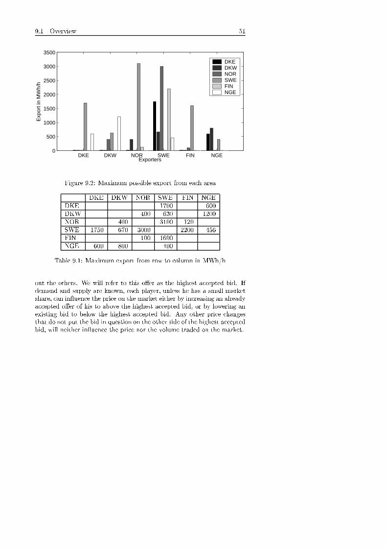
Figure 9.2: Maximum possible export from each area
DKE DKW NOR SWE FIN NGEDKE 1700 600DKW 400 630 1200NOR 400 3100 120SWE 1750 670 3000 2200 456FIN 100 1600NGE 600 800 400
Table 9.1: Maximum export from row to column in MWh/h
out the others. We will refer to this o�er as the highest accepted bid. Ifdemand and supply are known, each player, unless he has a small marketshare, can in�uence the price on the market either by increasing an alreadyaccepted o�er of his to above the highest accepted bid, or by lowering anexisting bid to below the highest accepted bid. Any other price changesthat do not put the bid in question on the other side of the highest acceptedbid, will neither in�uence the price nor the volume traded on the market.

52 Chapter 9. Characteristics of the Scandinavian electricity market
9.2 Competition and cooperation
The market can be divided into �ve areas (six including northern Germany)with limited transmission capacity between them. See �gure 9.2, where thecolumns indicate maximum export from each of the markets, and table 9.1.Let us imagine that all electricity generators in each of the areas are a singleplayer and the market is thus a game of six players. Each player then op-erates in a protected environment, where only limited competition can beemployed due to the transmission limitations of power between the areas.This does of course not hinder all competition, but strengthens the marketpower each player can wield in his own area. This seriously weakens thethreats that players can make to other players on other markets. Threatsare a way of getting others to cooperate or behave in a more convenientmanner. The transmission limitations decrease the likelihood of coopera-tion between players, as it is less enforceable and there are more limits towhat can be gained from international cooperation.
Example 9.1 If player A wants to punish player B in another market, hecan only do so if the price on his market is either above or the same asthe opponent's home market price. If the market price of A is higher thanthe market price of B, A must reduce his market price until it is as low asB's. When this has been accomplished, there is a common price area andboth players operate as if they were on the same market. From this point,A can economically punish B by reducing the price on the common market,but only as long as the market remains common, as once A has reducedhis price to a certain level, the price on market A becomes lower than onmarket B, and will no longer in�uence B's pro�t.
Therefore, interaction between players is limited to the transmission ca-pacities between them and when there are no longer any such capacitiesavailable, players will no longer be able to in�uence the prices on othermarkets. The player with more sales will usually lose more from pricereductions.
9.3 Demand
Although in general all suppliers will bene�t from raising their prices, givenstrict limitations on deviating from the current supply curve, suppliers with
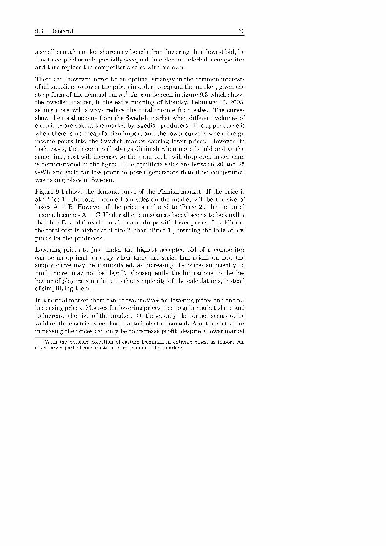
9.3 Demand 53
a small enough market share may bene�t from lowering their lowest bid, beit not accepted or only partially accepted, in order to underbid a competitorand thus replace the competitor's sales with his own.
There can, however, never be an optimal strategy in the common interestsof all suppliers to lower the prices in order to expand the market, given thesteep form of the demand curve.1 As can be seen in �gure 9.3 which showsthe Swedish market, in the early morning of Monday, February 10, 2003,selling more will always reduce the total income from sales. The curvesshow the total income from the Swedish market when di�erent volumes ofelectricity are sold at the market by Swedish producers. The upper curve iswhen there is no cheap foreign import and the lower curve is when foreignincome pours into the Swedish market causing lower prices. However, inboth cases, the income will always diminish when more is sold and at thesame time, cost will increase, so the total pro�t will drop even faster thanis demonstrated in the �gure. The equilibria sales are between 20 and 25GWh and yield far less pro�t to power generators than if no competitionwas taking place in Sweden.
Figure 9.4 shows the demand curve of the Finnish market. If the price isat `Price 1', the total income from sales on the market will be the size ofboxes A + B. However, if the price is reduced to `Price 2', the the totalincome becomes A + C. Under all circumstances box C seems to be smallerthan box B, and thus the total income drops with lower prices. In addition,the total cost is higher at `Price 2' than `Price 1', ensuring the folly of lowprices for the producers.
Lowering prices to just under the highest accepted bid of a competitorcan be an optimal strategy when there are strict limitations on how thesupply curve may be manipulated, as increasing the prices su�ciently topro�t more, may not be �legal�. Consequently the limitations to the be-havior of players contribute to the complexity of the calculations, insteadof simplifying them.
In a normal market there can be two motives for lowering prices and one forincreasing prices. Motives for lowering prices are: to gain market share andto increase the size of the market. Of these, only the former seems to bevalid on the electricity market, due to inelastic demand. And the motive forincreasing the prices can only be to increase pro�t, despite a lower market
1With the possible exception of eastern Denmark in extreme cases, as import cancover larger part of consumption there than on other markets

54 Chapter 9. Characteristics of the Scandinavian electricity market
0 1 2 3 4 5 6
x 104
0
0.5
1
1.5
2
2.5
3
3.5
4
4.5
x 107
MWh
Tot
al in
com
e
Income when full import
Income when no import
Maximum import to Sweden
Equilibrium when no import
Equilibrium when full import
Figure 9.3: Total hourly income from sales in Sweden
0 0.2 0.4 0.6 0.8 1 1.2 1.4 1.6 1.8 2
x 104
0
50
100
150
200
250
300
350
400
MWh
Uni
t pric
e in
NO
K
A
B
C
Price 1
Price 2
Demand
Figure 9.4: Demand in Finland

9.3 Demand 55
share and a smaller market. Having thus limited the factors that in�uencethe optimal strategy of each player, the problem should simpler.
However, as all electricity producers in certain areas (hopefully) do not actin unison to provide themselves with a monopolistic pro�t, but are likelyto compete, the strategy of raising prices or withholding production forplayers, especially those with small market share, is not necessarily prof-itable. This is why there is usually some competition, even on markets withfew competitors, although the competition may sometimes seem limited.Monopoly is usually not a Nash equilibrium unless with only one player.

56 Chapter 9. Characteristics of the Scandinavian electricity market

57
Chapter 10
Market power on Nord
Pool's spot market
10.1 Who could be using market power?
Market power has its price. When someone exercises market power, hedoes so in order to increase prices, but at the cost of sales. Thus, theuse of market power involves sacri�ces. In order for these sacri�ces to beworthwhile the e�ort and if pro�t is to be increased, enough market share,or merely sales, must remain to overcome the sales loss.
∆y × (x + ∆x) + y × ∆x +∫ x+∆x
x
S (x) dx ≥ 0 (10.1)
In the above formula, x and y respectively are the actual volume soldand the price, before the use of market power and S (x) is the supply orproduction cost function. ∆x and ∆y are the di�erence in sales and pricewhen market power is used. ∆x would be negative as less is sold, but∆y positive as the price will rise. The �rst component of the equation isthe increased revenue due to higher prices, the second component is lostrevenue due to less sales, and the third component, the integral, is thesaving in production cost due to less sales. If the sum of these items isgreater than zero, the use of market power will yield an increased pro�t
58 Chapter 10. Market power on Nord Pool's spot market
for the player in question. In �gure 9.4 the income part is explained andequation 10.1 may be rewritten as follows:
area B − area C + saving of production cost ≥ 0 (10.2)
As y, ∆y and ∆x will be the same for all players, the size of x will determinefor which players will be rewarded by the use of market power.
To be able to use market power, the players must be able to in�uenceprices. In order to do so, ∆x must be large enough. Sometimes the highestaccepted bid is large and only partially accepted. Thus, ∆x must be largerthan the unaccepted part of the highest accepted bid as well as less thanthe previous sales x.
The conclusion is that only big producers are likely to bene�t from usingmarket power.
10.2 Big producers
In the Scandinavian power market area, there are several large producerswith production which is often limited to only one of the markets. Theytend to have a large market share on their home market even though theirtotal market share in the combined market area may be modest.
In my calculations I will often consider the pro�t and opportunities of E2,Elsam, Statkraft, Vattenfall, Sydkraft, Fortum and E.On and refer to themas the 7 power players. In addition Elkraft and Eltra are large sellers ofelectricity, but being system operators in their own areas, they are notconsidered to exercise market power.
The largest power producers will now be brie�y discussed.
10.2.1 ENERGI E2
ENERGI E2 is a leading Danish production and energy trading company.They own and operate seven large power stations and eleven small ones aswell as CHP (Central heating plants) in eastern Denmark and hold sharesin a number of hydropower plants in Sweden and Norway. In addition tothis, E2 owns wind turbines in Sweden, Greece and Spain.

10.2 Big producers 59
The company was founded in June 2000 as the result of a merger betweenSK Power Company A/S, Københavns Energi Produktion A/S and EKEnergi Power Company A/S.
The aggregate electricity production at E2's generating facilities in Scandi-navia was 12.5 TWh in 2002. Wind power generated 0.4 TWh. Productionat the hydropower stations in Sweden amounted to 0.8 TWh. The majorpart of the remaining 11.3 TWh was produced at CHP plants in easternDenmark.
E2 has been increasing their share in wind power recently. Neither the newwindmills nor E2's shares in the Norwegian and Swedish hydropower plantsare represented in the data and are therefore omitted in the calculations.[16]
10.2.2 Elkraft
Elkraft is the transmission system operator in eastern Denmark and ownsmost of the high-voltage lines in the area. The company was establishedwhen the Danish electricity market was liberalized.
Although Elkraft does not produce electricity itself, Elkraft administers thedistribution of the environmentally friendly electricity that all electricityconsumers in Denmark must use. Elkraft is a non-pro�t company and isas such not supposed to exercise market power.[17]
10.2.3 Elsam
Elsam is the largest producer of electricity and district heating in Denmark.Elsam operates 6 central and 23 local CHPs as well as 486 windmills onJutland and Funen.[18]
10.2.4 Eltra
Eltra is the transmission system operator in Jutland and on Funen, and isresponsible for the overall security of supply in that area. Eltra bears theresponsibility for developing environmentally friendly electricity generationand incorporating it into the system. Eltra owns, develops and operatesthe 400 kV network as well as the connections to neighboring countries.

60 Chapter 10. Market power on Nord Pool's spot market
Besides this, Eltra manages the 150 kV network, forming part of the overallJutland-Funen transmission network.
In cooperation with other electricity supply undertakings and system op-erators in Denmark and abroad, Eltra is to contribute to developing andoperating the electricity supply industry e�ciently, while taking due con-sideration of security of supply, the national economy and the environment.
The new Danish Electricity Supply Act gives power stations, distributionundertakings and industrial customers (of a certain size) the right to freelyenter into agreements on purchase and sale of electricity in Denmark andabroad. It is an important task for Eltra to open the new electricity marketand make it work. This requires that the transmission network shouldbe expanded in accordance with market demand, that there should beopen, strong connections with the neighboring countries, that there shouldbe access to an e�cient power exchange, mirroring the market value ofelectricity at any time, and that all players should gain network access onuniform, nondiscriminatory terms.[3]
Eltra is a member of the Nord Pool spot market as it acts as an agent forsome windmill owners in western Denmark.
10.2.5 Statkraft
Statkraft is Norway's largest producer of hydroelectric power. Annual pro-duction capacity exceeds 42 TWh, about 1/3 of the country's hydroelec-tric power production. The company has around 2,500 employees, and is�rmly involved in developing power production based on renewable sources.Statkraft is state owned.
Statkraft holds a number of shares in the power industry in and outsideScandinavia. The most signi�cant is Statkraft's 44% ownership of sharesin the Swedish Sydkraft.
Statkraft is also engaged in power trading all over northern Europe.[19]
10.2.6 Vattenfall
Vattenfall is the state owned electricity producer in Sweden. It operateshydro, nuclear and thermal plants in Sweden, Finland and Germany. Priorto deregulation, Vattenfall operated the Swedish national grid.

10.2 Big producers 61
Vattenfall has acted as a developer, investor and long-term partner in powerprojects located mainly in South East Asia and Latin America. [20]
10.2.7 Sydkraft
The Sydkraft Group consists of 60 operating subsidiaries. Approximately5,300 employees handle electricity sales, electricity distribution, electricityproduction, natural gas, LPG, heat, cooling, water and sewage systems andenergy, material recovery from waste, energy trading and communicationsolutions. These companies, together with a number of Group managementfunctions, form a complete energy group.
Amongst other things, Sydkraft operates nuclear plants, hydro plants andCHPs. Most of them are situated in Sweden.
E.On in Germany owns 56% of Sydkraft against Statkraft's 44% share. Inmy calculations I will not take these ownerships into account.[21]
10.2.8 Fortum
Fortum is the second largest electricity producer in Scandinavia as well asbeing a leading energy company in other parts of the Baltic Rim. Fortum'sactivities cover the generation, distribution and sale of electricity and heat,the production, re�ning and marketing of oil, the operation and mainte-nance of power plants as well as energy-related services. The main productsare electricity, heat and steam as well as tra�c fuels and heating oils.
Fortum owns wholly or partly over 500 power plants in central Sweden,Greater Stockholm and in various parts of Finland. 60% of its power gen-eration is renewable and over 80% carbon dioxide free. Fortum uses hydro,wind and nuclear power, coal, natural gas, peat, biomass and oil as energysources.[22]
10.2.9 E.On
E.On is a German energy group which operates mainly in Germany. E.Onis Europe's largest provider of energy services. E.On owns 56% of theSwedish Sydkraft.[23]

62 Chapter 10. Market power on Nord Pool's spot market
10.3 Winners and losers
Having identi�ed the most probable users of market power, knowing whichones are there to gain and which ones are there to lose, may be important.
Those who might gain from the use of market power are:
1. The users of market power, otherwise they would not be using it.They will bene�t from higher prices despite less sales.
2. Other producers. They will gain all the bene�ts from higher prices,without having to pay the cost involved with less sales. Peer pressuremight help.
3. Grid line operators may gain from increased price di�erences betweenmarkets.
There are also a few on the losing side.
1. Sellers of electricity to end users, as they will either have to bear thehigher cost or face less sales.
2. The public, which will have to pay higher bills.3. The business will also have to pay more and that means less business.4. The state. Less business means less taxes, and an unhappy public
leads to fewer votes.5. Nord Pool. Less credibility will a�ect their status. Nord Pool will not
want its market to be considered the breeding place of monopolisticpro�t at the cost of the common good.
As a result, market power users may face formidable opponents.
10.4 The rules of the game
These are the ethical guidelines signed by all players of the Nord Pool spotmarket:[24]
1. All transactions made in Nord Pool's markets shall be performed witha genuine and generally acceptable business purpose.
2. No �ctive transactions and mock agreements shall be carried out,and Participants and Clearing Customers must never give false ormisleading expressions of their intentions with trades or bids ando�ers in the markets.

10.5 As time goes by 63
3. No bids or o�ers or trades shall be presented to the market with thepurpose of misleading other Participants and Clearing Customers.Sudden changes in market behaviour that is not motivated by seriouscommercial or technical circumstances must not occur.
4. Any Participant or Clearing Customer that is a leading player inrespect to the relevant supply or demand for electricity or electricityderivatives must assure that they do not in any inconsiderate waya�ect the price development in the relevant markets.
5. No misleading information must be given that can contribute to makea false and incorrect or misleading picture of the market situation.
These could be summarized into one commandment: Thou shall not exer-cise market power!
If we assume that everybody is follows these guidelines, we have nothingto worry about. On the other hand, it is human to err.
10.5 As time goes by
Market power can be used either to exploit a short term position or to maxi-mize the expected long time pro�t. As there are often short term variationsin prices, it could be very pro�table to react immediately to opportunitiesas they arise. However, due to the restrictions imposed on players, as out-lined in section 10.4, this can often be impossible as �serious commercial ortechnical circumstances� may not always occur when convenient, e.g. whenwindfall is expected during peak consumption hours, there is a failure in alarge power plant etc., or when someone has recently started underbidding.Thus, players may rather want to focus on expected long term forecasts ofthe market and choose strategy, although in�exible, which will maximizetheir pro�t given their limited scope of operations.
10.6 How can market power be exercised?
The ultimate purpose of market power is to make more pro�t throughhigher prices, despite less sales. But there are a few paths to this goal. Onthe Scandinavian electricity market, the following are the most obvious:
• Raising prices

64 Chapter 10. Market power on Nord Pool's spot market
• Withholding production• Wrong predictions• Blocking grid lines• Cooperation• Leaving the spot market
Each of these elements will be discussed further in the following sections.
10.6.1 Raising prices
The most straight forward use of market power is simply to raise prices.However, due to the restrictions on market behavior, it is di�cult to ex-ploit at least the short term use of price raising. However, for long termopportunities, justi�cation will be found for raising prices when the price offuel goes up, unfortunate exchange rates develop, wages increase etc.; all ofwhich is sometimes forgotten when circumstances become more favorableagain. Then there is the question of the pricing of hydroelectricity. Thismakes changing prices con�ned mainly to long term use of market power.
When a player increases the price of his production, part of the supplyfunction will rise and this may cause the order of o�ers to change. Thesystem price will always increase equal or less to the player's increase. Thereasons for this are:
• Demand is �exible. When prices rise, less will be sold.• To in�uence prices, the producer must have o�ered such a high priceto his accepted bids that after the rise, some of his o�ers will behigher than the former system price.
• The o�ers which rise above the old market price may be replaced withformerly unaccepted bids from other players, which now become lowerthan the player's bids.
• If the highest accepted bid is not wholly accepted, raising prices abovethe highest bid may thus not increase prices, as the bids, that roseabove the highest accepted bid will be replaced with the unacceptedpart of that bid.
Example 10.1 If the demand is entirely in�exible and a player owns allbids on the market that are 5% above or below the system price, a 5%increase in the price would cause the system price to increase by 5% aswell.

10.6 How can market power be exercised? 65
Price strategies will be discussed further in chapter 11.
To demonstrate the possibilities of increasing pro�t, tests were run on thee�ect of the 7 power players' pro�t when they change the markup on theirhome market from 0% to 10%.1 The data is from Eltra and is for peakconsumption from 11 am to 12 pm on Tuesday, February 11, 2003. Whenno player is exercising market power, the market may be divided into twoprice areas: on the one hand western Denmark and northern Germany withprice around NOK 155 per MWh and on the other hand the other marketswith prices around NOK 207.
1 1.01 1.02 1.03 1.04 1.05 1.06 1.07 1.08 1.09 1.1−2500
−2000
−1500
−1000
−500
0
500
Markup
Cha
nge
in p
rofit
E2ElsamStatkraftVattenfallSydkraftFortrumEon
Figure 10.1: Tuesday: Changes in Elsam's pro�t with di�erent markups
Neither E2 nor Statkraft succeeded in changing the prices on their marketas they were not able to, raise any of their bids above the highest acceptedbid, given the limited markup allowed, and are thus not demonstrated.Elsam and Fortum, �gures 10.1 and 10.6, could not in�uence prices to anyextent, but lost sales to others, and thus did not pro�t from their adventure.Sydkraft, �gures 10.4 and 10.5, succeeded in changing the market price, butthe all the bene�t went to other players. However, Vattenfall and E.On weresuccessful in increasing their (and other players') pro�t. See �gures 10.2,10.3, 10.7 and 10.8.
1Eltra has suggested maximum markup being between 5% and 10%

66 Chapter 10. Market power on Nord Pool's spot market
1 1.01 1.02 1.03 1.04 1.05 1.06 1.07 1.08 1.09 1.10
1
2
3
4
5
6
7
8
9
10x 10
4
Markup
Cha
nge
in p
rofit
E2ElsamStatkraftVattenfallSydkraftFortrumEon
Figure 10.2: Tuesday: Changes in Vattenfall's pro�t with di�erent markups
1 1.01 1.02 1.03 1.04 1.05 1.06 1.07 1.08 1.09 1.1150
160
170
180
190
200
210
220
Markup
Pric
e of
MW
h
DKEDKWNORSWEFINNGE
Figure 10.3: Tuesday: Prices when Vattenfall changes its markup

10.6 How can market power be exercised? 67
1 1.01 1.02 1.03 1.04 1.05 1.06 1.07 1.08 1.09 1.1−2
−1
0
1
2
3
4
5
6x 10
4
Markup
Cha
nge
in p
rofit
E2ElsamStatkraftVattenfallSydkraftFortrumEon
Figure 10.4: Tuesday: Changes in Sydkraft's pro�t with di�erent markups
1 1.01 1.02 1.03 1.04 1.05 1.06 1.07 1.08 1.09 1.1150
160
170
180
190
200
210
220
Markup
Pric
e of
MW
h
DKEDKWNORSWEFINNGE
Figure 10.5: Tuesday: Prices when Sydkraft changes its markup

68 Chapter 10. Market power on Nord Pool's spot market
1 1.01 1.02 1.03 1.04 1.05 1.06 1.07 1.08 1.09 1.1−10000
−8000
−6000
−4000
−2000
0
2000
4000
Markup
Cha
nge
in p
rofit
E2ElsamStatkraftVattenfallSydkraftFortrumEon
Figure 10.6: Tuesday: Changes in Fortum's pro�t with di�erent markups
1 1.01 1.02 1.03 1.04 1.05 1.06 1.07 1.08 1.09 1.10
1
2
3
4
5
6
7x 10
4
Markup
Cha
nge
in p
rofit
E2ElsamStatkraftVattenfallSydkraftFortrumEon
Figure 10.7: Tuesday: Changes in E.On's pro�t with di�erent markups

10.6 How can market power be exercised? 69
1 1.01 1.02 1.03 1.04 1.05 1.06 1.07 1.08 1.09 1.1150
160
170
180
190
200
210
Markup
Pric
e of
MW
h
DKEDKWNORSWEFINNGE
Figure 10.8: Tuesday: Prices when E.On changes its markup
According to this data, by increasing their markup by ca. 10% and there-with the system price in the area by ca. 5%, Vattenfall could increase theirpro�t by ca. NOK 9,500 per hour, which would on a yearly basis sum upto NOK 83,220,000.
However, just 33 hours earlier, in the early morning of Monday, February10, 2003, we have a di�erent situation. Here there are three price areaswith western Denmark at ca. NOK 132, eastern Denmark and Germany atNOK 154 and the rest at NOK 192 per MWh.
All players can, at this time, bene�t from exercising market power, butsome only modestly and with only a small markup, while others can cashin an extra handsome pro�t with a substantial markup. The Danes do wellduring the night: E2, �gures 10.9 and 10.10, after they succeed in break-ing away from the Germans and forming its own price area, and Elsam,�gures 10.11 and 10.12, increases pro�t gradually with increased prices. Inthe north, prices change less, although Statkraft, with maximum markupin the end, succeeds in leaving the Finns behind, �gure 10.14. However,Statkraft, Vattenfall, Sydkraft and Fortum, �gures 10.13 to 10.17, onlyseem to bene�t from modest markup as the rest of the pro�t goes to thecompetitors. E.On only manages to increase prices insigni�cantly, and is

70 Chapter 10. Market power on Nord Pool's spot market
thus not demonstrated.
1 1.01 1.02 1.03 1.04 1.05 1.06 1.07 1.08 1.09 1.1−4000
−2000
0
2000
4000
6000
8000
10000
12000
Markup
Uni
t pric
e in
NO
K
E2ElsamStatkraftVattenfallSydkraftFortrumEon
Figure 10.9: Monday: Changes in E2's pro�t with di�erent markups
1 1.01 1.02 1.03 1.04 1.05 1.06 1.07 1.08 1.09 1.1130
140
150
160
170
180
190
200
Markup
Pric
e of
MW
h
DKEDKWNORSWEFINNGE
Figure 10.10: Monday: Prices when E2 changes its markup

10.6 How can market power be exercised? 71
1 1.01 1.02 1.03 1.04 1.05 1.06 1.07 1.08 1.09 1.10
0.5
1
1.5
2
2.5x 10
4
Markup
Cha
nge
in p
rofit
E2ElsamStatkraftVattenfallSydkraftFortrumEon
Figure 10.11: Monday: Changes in Elsam's pro�t with di�erent markups
1 1.01 1.02 1.03 1.04 1.05 1.06 1.07 1.08 1.09 1.1130
140
150
160
170
180
190
200
Markup
Pric
e of
MW
h
DKEDKWNORSWEFINNGE
Figure 10.12: Monday: Prices when Elsam changes its markup

72 Chapter 10. Market power on Nord Pool's spot market
1 1.01 1.02 1.03 1.04 1.05 1.06 1.07 1.08 1.09 1.1−3
−2
−1
0
1
2
3
4
5x 10
4
Markup
Cha
nge
in p
rofit
E2ElsamStatkraftVattenfallSydkraftFortrumEon
Figure 10.13: Monday: Changes in Statkraft's pro�t with di�erent markups
1 1.01 1.02 1.03 1.04 1.05 1.06 1.07 1.08 1.09 1.1130
140
150
160
170
180
190
200
Markup
Pric
e of
MW
h
DKEDKWNORSWEFINNGE
Figure 10.14: Monday: Prices when Statkraft changes its markup

10.6 How can market power be exercised? 73
1 1.01 1.02 1.03 1.04 1.05 1.06 1.07 1.08 1.09 1.10
0.5
1
1.5
2
2.5
3x 10
4
Markup
Cha
nge
in p
rofit
E2ElsamStatkraftVattenfallSydkraftFortrumEon
Figure 10.15: Monday: Changes in Vattenfall's pro�t with di�erentmarkups
1 1.01 1.02 1.03 1.04 1.05 1.06 1.07 1.08 1.09 1.10
1000
2000
3000
4000
5000
6000
7000
8000
Markup
Cha
nge
in p
rofit
E2ElsamStatkraftVattenfallSydkraftFortrumEon
Figure 10.16: Monday: Changes in Sydkraft's pro�t with di�erent markups

74 Chapter 10. Market power on Nord Pool's spot market
1 1.01 1.02 1.03 1.04 1.05 1.06 1.07 1.08 1.09 1.1−2000
−1000
0
1000
2000
3000
4000
5000
6000
Markup
Cha
nge
in p
rofit
E2ElsamStatkraftVattenfallSydkraftFortrumEon
Figure 10.17: Monday: Changes in Fortum's pro�t with di�erent markups
One can see how di�erent markups will maximize pro�t at each time, whichmay complicate the price strategy of players as a price strategy cannot beeasily altered. It is also worth emphasizing in these examples that when aplayer changes his markup, new markups may be optimal for other players.
10.6.2 Withholding production
The second most common form of market power is withholding production.Production can be withheld in several ways. The following may be the mostobvious:
Maintenance of powerplants Outage, during necessary or unnecessarymaintenance, can be pro�table.
Outages and errors Sometimes powerplants simply fail to function. Itcan be very human to err.
Closing down Permanent closing of old and unpro�table (indeed) powerplants.
Lack of investment Not building new plants, although they would bemore cost e�cient than the old ones. If it can be pro�table to close

10.6 How can market power be exercised? 75
down e�cient power plants for maintenance, building new ones, wouldnot be wise.
Cautious estimate of wind power O�ering less wind power than is ex-pected would be the same as withholding power from the market. Asit is usually more expensive for producers to buy extra power whenproduction falls short of predictions than the loss in sales when toolittle is predicted, it seems natural for producers to promise no morethan they can be somewhat certain of being able to deliver, which isthen less than the expected value of power generated.
Cautious estimate of water reservoir prospects Production from hy-dropower plants that rely on water reservoirs, may often be withheldto avoid water shortage later on; which may lead to shortage of elec-tricity with rationing and dramatic increases in prices. Therefore, itseems to be in the interest not only of producers but also consumersthat cautious estimates are made of the water reservoirs to minimizethe danger of water shortage, and it is thus better to err on the sideof caution. But how much to �err" may be a matter of opinion.
Withholding production shifts a part of the supply curve to the right. Thepart that shifts are all the o�erings which were higher than the o�er with-held. Under certain circumstances small shifts may cause a considerableincrease in the system price when demand is inelastic and more expensivepower, than the old system price, must consequently be produced to replacethe power withheld.
In order to check whether withholding production may be pro�table, testswere run for each of the 7 power players, when their highest, but never-theless accepted bids in case of full production, were withdrawn. Up to1000 MWh/h were thus withheld on each player's home market. Sales didnot, however, necessarily drop by the same volume, as bids, which other-wise would not have been accepted, were sometimes reduced to minimizeproduction cost.
Figures 10.18 to 10.24 demonstrate the e�ect on income, cost and pro�tfor the data from Eltra between 11 am to 12 pm on Tuesday, February11, 2003. Withholding up to 1000 MWh per hour is certainly impossiblefor some of the players, but the �gures give us an idea of what could beaccomplished. The income and cost have been divided by 10 in order togive a better view of the pro�t.
The Danes will lose from withholding production, whereas Statkraft, Vatten-fall, Sydkraft, Fortum and E.On will pro�t. E.On starts to make insigni�-

76 Chapter 10. Market power on Nord Pool's spot market
0 100 200 300 400 500 600 700 800 900 1000−7
−6
−5
−4
−3
−2
−1
0x 10
4
Uni
t pric
e in
NO
K
MWh
ProfitIncomeCost
Figure 10.18: Tuesday: Hourly change in E2's pro�t when production iswithheld
0 100 200 300 400 500 600 700 800 900 1000−1.5
−1
−0.5
0
0.5
1
1.5
2x 10
4
Cha
nge
in p
rofit
in N
OK
MWh
ProfitIncomeCost
Figure 10.19: Tuesday: Hourly change in Elsam's pro�t when productionis withheld

10.6 How can market power be exercised? 77
0 100 200 300 400 500 600 700 800 900 1000−2
−1
0
1
2
3
4x 10
4
Cha
nge
in p
rofit
in N
OK
MWh
ProfitIncomeCost
Figure 10.20: Tuesday: Hourly change in Statkraft's pro�t when productionis withheld
0 100 200 300 400 500 600 700 800 900 1000−4
−2
0
2
4
6
8
10
12x 10
4
Cha
nge
in p
rofit
in N
OK
MWh
ProfitIncomeCost
Figure 10.21: Tuesday: Hourly change in Vattenfall's pro�t when produc-tion is withheld

78 Chapter 10. Market power on Nord Pool's spot market
0 100 200 300 400 500 600 700 800 900 1000−2
−1.5
−1
−0.5
0
0.5
1
1.5
2x 10
4
Cha
nge
in p
rofit
in N
OK
MWh
ProfitIncomeCost
Figure 10.22: Tuesday: Hourly change in Sydkraft's pro�t when productionis withheld
0 100 200 300 400 500 600 700 800 900 1000−2
−1.5
−1
−0.5
0
0.5
1x 10
4
Cha
nge
in p
rofit
in N
OK
MWh
ProfitIncomeCost
Figure 10.23: Tuesday: Hourly change in Fortum's pro�t when productionis withheld

10.6 How can market power be exercised? 79
0 100 200 300 400 500 600 700 800 900 1000−2
0
2
4
6
8
10
12
14x 10
4
Cha
nge
in p
rofit
in N
OK
MWh
ProfitIncomeCost
Figure 10.24: Tuesday: Hourly change in E.On's pro�t when production iswithheld
cantly more pro�t when withholding 400 MWh/h or more.
Figures 10.25 and 10.26 show the pro�t of each player for the data fromthe 1st hour of Monday, February 10, 2003.
The Danes start to make a handsome pro�t when withholding ca. 500MWh/h; E2 after considerable loss up to that time. Other players makeless pro�t, except Fortum which always seems to lose. Notice the frequentsmall steps in the pro�t of Statkraft, Vattenfall, Sydkraft and Fortum.
Withholding wind power will be less pro�table than withholding more ex-pensive power, although withholding the latter may be easier. In �gure10.27 the optimal production for can be seen for Elsam at the two datadates. Actual production was 335 and 304 MWh for Monday and Tuesdayrespectively, windy days, but the dream production for Elsam would be850 MWh on Monday and even more on Tuesday, both being more thanthey can deliver with the current installations.

80 Chapter 10. Market power on Nord Pool's spot market
0 100 200 300 400 500 600 700 800 900 1000−2
−1
0
1
2
3
4
5
6
7x 10
4
MWh
Cha
nge
in p
rofit
in N
OK
E2ElsamStatkraftVattenfallSydkraftFortrumEon
Figure 10.25: Monday: Hourly change in pro�t when production is withheld
50 100 150 200 250 300 350 400 450 500
−2000
−1000
0
1000
2000
3000
4000
5000
MWh
Cha
nge
in p
rofit
in N
OK
E2ElsamStatkraftVattenfallSydkraftFortrumEon
Figure 10.26: Monday: A closer look at pro�t

10.6 How can market power be exercised? 81
0 500 1000 1500−5
0
5
10
15
20x 10
4
MWh
Uni
t pric
e in
NO
K
Sunday morningMonday noon
Figure 10.27: Optimal wind power production for Elsam
10.6.3 Wrong predictions
The line between being cautious and imprudent may be di�cult to follow.O�ering less than expected at the spot market can be accepted to a certainlimits, but to what extent? Predictions may always be wrong, but theycan also be made wrong.
It is less expensive to be wrong about the water reservoir level than aboutthe wind power. Wind power withheld is lost, blown away, while the watermay be kept and put to use later, which may be a drawback to marketpower users, as this may cause lower prices later on.
Surplus wind power can be put to some use. It can replace the moreexpensive production of the same player, which in reality allows the playerto rate some of his expected wind power, much higher than otherwise, ase.g. expensive gas turbines may be replaced. The surplus may also be soldto other producers who may �nd it convenient to buy inexpensive powerfor reselling rather than producing expensive power themselves.
Finally, in Denmark there are plans to use surplus wind power for heatingwater for central heating. This may lead to a smaller supply of cheap CHP

82 Chapter 10. Market power on Nord Pool's spot market
power during the following hours or day when less heating carried out, tothe delight of most producers. The use of an unpredictable surplus windpower to heat water requires the existence of large insulated water tanks.
All possible use of cheap surplus wind power contributes to making windpower �predictions� an instrument of market power.
When wind power can be used to replace more expensive production, thee�ect is the same as when withholding the most expensive production.As can been seen in �gures 10.19 and 10.26, Elsam would bene�t frompredicting 0 instead of the 334 MWh on Monday (and thus withhold 334MWh of expensive power) but needs to produce more wind power to beable to exploit the situation on Tuesday, and Elsam should therefore putforth a correct �prediction.�
10.6.4 Blocking grid lines
One aspect of market power would be to block cheap power from othermarkets from �owing into the more expensive markets, with the consequentprice reduction. If the line between two markets is blocked, this will causehigher a price on one of the markets and a lower price on the other market.
Blocking grid lines will not be as popular with other players as is thetraditional exercise of market power, as producers in cheap markets willnot be able to sell power abroad, in addition to su�ering lower prices onthe home market. The blocking player will instead acquire, with other localproducers, protection from foreign competition which will increase priceson his market.
In �gures 10.28 to 10.30 we see how players' pro�t would be a�ected shouldthe grid line between eastern Denmark and Sweden be blocked on Tuesday,February 11, 2003. When the grid line is not blocked, eastern Denmarkforms a price area with the northern markets. However, when the line isblocked, prices in eastern Denmark tumble and eastern Denmark becomesits own price area as the cheapest power market, to the delight of Danishconsumers, but the wrath of E2. Vattenfall would have the most to gainby the blocking.
Certain changes in regulations regarding reservations of grid lines haverecently by made to hinder the blocking of international grid lines. I amnot familiar with how blocking can currently be done, and will therefore

10.6 How can market power be exercised? 83
0 200 400 600 800 1000 1200 1400 1600 1800−16
−14
−12
−10
−8
−6
−4
−2
0
2
4x 10
4
Cha
nge
in p
rofit
in N
OK
MWh
E2ElsamStatkraftVattenfallSydkraftFortrumEon
Figure 10.28: Turning o� eastern Denmark
0 200 400 600 800 1000 1200 1400 1600
−0.5
0
0.5
1
1.5
2
2.5
3
3.5
4
x 104
Cha
nge
in p
rofit
in N
OK
MWh
E2ElsamStatkraftVattenfallSydkraftFortrumEon
Figure 10.29: A closer look at the Sound connection

84 Chapter 10. Market power on Nord Pool's spot market
0 200 400 600 800 1000 1200 1400 1600 1800140
150
160
170
180
190
200
210
MWh
Uni
t pric
e in
NO
K
DKEDKWNORSWEFINNGE
Figure 10.30: Prices when holding up the line
not discuss this method further in this thesis. This has only pointed outas a possibility.
10.6.5 Cooperation
Cooperation between players can be either active or inactive. Active coop-eration would include a formal or more likely an informal and secret dealbetween players concerning market behavior and the division of pro�t fromthe use of market power.
Inactive cooperation could be not to use opportunities to lower prices, eventhough more pro�t could be gained at least temporarily, or to increaseprices in the hope that other players will follow, which would be inactivecooperation from their side.
Cooperation in itself is not market power. However, cooperation magni�esthe bene�ts of using other methods of market power as larger market shareand greater price control will be gained and exploitation of the situationfrom, now fewer, competitors will be reduced.
When examining �gure 10.31 where the Tuesday data is used, we can see

10.6 How can market power be exercised? 85
that Elkraft, which is not one of the power players, would want to produceca. 500 MWh/h if it is not able to produce at least 800 MWh/h. However,if Elkraft and E2 were cooperating and thought of maximizing their totalpro�t, Elkraft would never want to produce more than 500 MWh/h unlessbeing able to deliver at least 1500 MWh/h.
0 500 1000 1500−1.5
−1
−0.5
0
0.5
1
1.5
2x 10
5
MWh
Cha
nge
in p
rofit
in N
OK
Elkraft E2 Total profit
Figure 10.31: Optimal wind power production
10.6.6 Leaving the spot market
By making long term contracts with prominent buyers, a producer candecrease trade on the Nord Pool spot market, although in theory the longterm buyers could resell their power on the spot market, and thus make themarket more shallow and less liquid, with fewer participants on both sides.According to Nord Pool, trade on the spot market has been increasing inrecent years and currently there seems to be no reason for concern regardingdecline in trade in the near future.

86 Chapter 10. Market power on Nord Pool's spot market
10.7 Detecting market power
Having de�ned some of the possible forms of market power, one might beinterested in �nding out whether any of it is being used.
10.7.1 By whom?
Firstly, one must decide who would be trying to detect the market power.The most likely are those which in section 10.3 were referred to as the`losers.' These are the foremost:
• Nord Pool• Transmission system operators• Competition institutions and authorities
Of the above, Nord Pool is by far in the best position as they are the onlyparty that will know the exact bidding of all the electricity generators.Other parties must be satis�ed with �lling into the blanks with guessesand models.
The true production cost is then, of course, only available to the power plantowners, making all assumptions of market power based on assumptions ofproduction cost.
Finally, there are the water reservoirs with their complex pricing.
10.7.2 And how?
The following are what detectors should be monitoring:
Outage Does the player bene�t? Are outages more frequent than ex-pected?
Size Does the player have a large market share?Predictions Does the player bene�t from predicting too little wind en-
ergy? Is there systematic undervaluing in predictions?Water reservoirs Is the water reservoir situation as critical as hydropower
generators may claim?Grid lines Are grid lines reserved, and, if that is the case, are they being
used?

10.7 Detecting market power 87
Fuel cost Does the price of electricity from coal, oil and gas sources go upwith the price of the raw materials, but not down again?
Price Is the price simply too high compared to models? Are there Nashequilibria or is there cooperation with Pareto optimal solution?
Being alert and searching for pattern in behavior is probably most e�cientway of market detection.

88 Chapter 10. Market power on Nord Pool's spot market

89
Chapter 11
Price strategies
11.1 Overview
There are a few possible circumstances on the market. In the followingsections, these will be discussed and analyzed for optimal response. Underall these circumstances the highest accepted bid is the crucial factor asit sets the price and we assume, for simplicity's sake, strict limits to howthe supply curve may be manipulated and that no player can reduce hisbid to a lower price than any of his other originally lower prices. I.e. hecannot lower two bids to below a price both bids were above before. Havingsaid that, it leaves us with two important bids for each player, his highestaccepted bid and his lowest unaccepted bid. If the player holds the highestaccepted bid on the market, and the bid is only partially accepted, this bidfunction as both the highest accepted and the lowest unaccepted bid.
To heighten the market price, a player must increase his highest acceptedbid until the bid is either no longer accepted, or only partially accepted.In order to sell more, a player must lower his lowest unaccepted bid tobelow the highest accepted bid. Whether increasing or decreasing priceswill bene�t the player depends on his market share, his markup and theelasticity of demand.

90 Chapter 11. Price strategies
11.2 Export and import
When the export capacity between two or more markets is not fully utilized,they have the same price and therefore form a single price area. The sameprice is on all the markets and they function as a single market until allthe transmission capacity has been used, either by lowering or heighteningthe price of the local supply.
When there is a di�erent price between two markets and there is full use oftransmission capacity between them, the supply line of the more expensivemarket gets the addition of the same volume as the transmission capacitybetween the markets. The supply of the cheaper market is reduced by thesame volume.
Example 11.1 The market price in Norway is 190 and 175 in Sweden, butwould have been 200 in Norway and 165 in Sweden if no export had takenplace. This is demonstrated in �gure 11.1, where the broken lines representsupply and demand in Sweden after export and the continuous lines are thedemand and supply in Norway after import. The dotted line is the demandin both Sweden and Norway before transmission (the same demand is usedto keep the diagram less crowded), which is then shifted 100 MWh to theright for Sweden and 100 MWh to the left for Norway as 100 MWh areexported from Sweden to Norway. N1 and N2 are the prices and volume inNorway before and after import respectively, S1 and S2 are the prices andvolume in Sweden before and after export.
This shift of the demand curve will give us the right market price and thecorrect amount of power produced in each area, but not the correct con-sumption in each area. If the supply curves had been shifted in the oppositedirections, Norwegian to right and Swedish to left, correct prices and con-sumption could be read from the �gure. This is because consumption andproduction can not be equal in markets where import or export is takingplace.
However, this approach of shifting the whole curves is not entirely accurate.It would be more accurate to transfer the most expensive supply producedfrom the Swedish supply curve and add it to the Norwegian supply curve.There it would form a part of the new Norwegian supply curve, but wouldcause the same shift to the right at and above the Norwegian market price,as all imported Swedish supply would be cheaper than the market price;as otherwise it would not be imported. Thus, the new Swedish supply can

11.3 Selecting a strategy 91
0 50 100 150 200 250 300 350 400 450 500100
150
200
250
MWh
Uni
t pric
e in
NO
K
N1
S1
N2
S2
Figure 11.1: E�ects of export/import on prices in Norway and Sweden
become the second highest accepted or even the highest (fully, as otherwisethere would be the same market price and a single price area) accepted bidon the Norwegian market.
The same is also true for the shift of the Swedish demand when the Norwe-gians start buying. The part of the Norwegian demand curve immediatelyto the right of the old market price would be shifted to Sweden to forma part of the new Swedish demand curve. Thus, both Swedish and Nor-wegian producers only have to take a look at their own modi�ed demandand supply curves and do not have to observe other markets when decidingtheir own price strategies, as all the important information is to be foundon the demand and supply curves in their own price area.
11.3 Selecting a strategy
11.3.1 Highest accepted bid
When a player holds the highest accepted bid, it means that unless he alsoholds the lowest unaccepted bid, other players may be tempted to challenge

92 Chapter 11. Price strategies
this bid. The bid can either be fully or only partially accepted. See �gure11.2.
0.5 0.6 0.7 0.8 0.9 1 1.1 1.2 1.3 1.4 1.5 1.6
x 104
0
100
200
300
400
500
600
MWh
Pric
e in
NO
K
Lowest unaccepted bid
2nd highest accepted bid
Highest accepted bid
Figure 11.2: Supply and demand on the Finnish market
11.3.2 Fully and partially accepted bids
If the highest accepted bid is fully accepted, as in �gure 11.3, the holderof the bid has nothing to gain by reducing his price and thus underbiddingother players as he would not be selling any more. He can, however, takeadvantage of the fact that the market price will not decrease when helowers his prices and thus reduce the likelihood of underbidding from otherplayers. In order to heigthen the market price, the player must increaseprices until not all of his bid is accepted. From there he may increase themarket price if pro�table. Only when the highest accepted bid is partiallyaccepted will raising or lowering it a�ect the market price and sales, andthus that player's pro�t.

11.3 Selecting a strategy 93
2500 3000 3500 4000 4500 50000
50
100
150
200
250
300
350
400
450
MWh
Uni
t pric
e in
NO
K
Highest accepted bid
All of the bid is accepted
Figure 11.3: Demand and supply in western Denmark
11.3.3 Second highest accepted bid
The holder of the second highest accepted bid is only under threat from theholder of the highest accepted bid, if not all of the highest accepted bid wasaccepted, as otherwise the holder of the highest bid would have nothing togain by underbidding nor would the holder of the second highest acceptedbid have anything to lose. If possible, that player should lower his bid tobelow the production cost of the highest accepted bid or at least maintaina gap between his bid and the highest accepted one. He should do so inorder to discourage underbidding, especially if a large part of the highestaccepted bid is only partially accepted. The holder of the second highestaccepted bid can never bene�t from increasing that bid while below themarket price.
11.3.4 Lowest unaccepted bid
The holder of the lowest unaccepted bid is always in position to challengethe highest accepted bid. If all of the highest accepted bid was accepted,that player can increase sales without underbidding the currently highest

94 Chapter 11. Price strategies
accepted bid by lowering his bid to below the market price, but nonethelessstaying above the highest accepted bid. That will, however, cause a marketprice reduction, as will all additional sales. This player could also underbidthe highest accepted bid, but he should only do so if his production costis lower than the production cost of the highest accepted bid, unless theholder of the highest accepted bid is not expected to react.
As the bidding blocks are often quite large, players will always gain byreducing their prices to just below the competitor, until they reach theirown production cost, and gain some extra sales as their bid will replacethe bid of the competitor. Therefore, players should never try to underbidbids with lower production cost, as this will most likely only cause lowermarket price while probably selling nothing or just a little more. This isdemonstrated in �gure 11.4.
−20 −15 −10 −5 0 5 10
−10
−5
0
5
10
Cha
nge
in p
rofit
Deviation in price
Current price
Highest accepted bid
Highest accepted bid replaced
Successful underbidding
Unsuccessful underbidding
Marginal cost of bid
Figure 11.4: Gains and losses for the holder of the lowest unaccepted bid
In �gure 11.4, a player holds, in the beginning, the lowest unaccepted bid,de�ned as zero on the x axis, at NOK 10 above the highest partially ac-cepted bid and the market price, and NOK 17 above his marginal cost. Ifthe player now lowers the price of his bid, his pro�ts will be constant untilhis bid becomes lower than the highest accepted bid. His pro�t will then in-crease, but only if the other player does not in turn lower his price. Hence,there are two pro�t lines: one showing the player ending with lower bid

11.3 Selecting a strategy 95
than the competitor, and the other, the broken one, showing when the com-petitor prevailing with the lower bid. While the continuous line stays abovethe broken line, the player will gain by reducing his price to just below thecompetitor, provided that the competitor has underbid him. Indeed, hewill constantly be shifting between the two pro�t lines as the competitorreacts and counter-reacts, starting a downward price spiral. This is, how-ever, only true until the player reaches his own marginal production cost,as, from that time onward, he will lose more by prevailing with the lowerbid and thus sell his power at below marginal cost. Thus, before the playerstarts underbidding others, he should be certain of being able to win theprice war, which is only possible should the competitor either not respondor have higher marginal production cost.
If the highest bid had been fully accepted, the competitor would have beenwise to keep his price below the marginal production cost of the player asexplained before, as he would not cause a lower market price, while avoidingthe price war.
A wiser move for the holder of the lowest unaccepted bid, if he has a higherproduction cost than the highest partially accepted bid, would therefore benot to underbid the competitor but to increase his price. This may temptthe competitor to raise his price too, leading to higher market price and ahigher pro�t, at least for the player.
This is an example of when a solution that is not a Nash equilibrium butPareto optimal, prevails.
11.3.5 Power players
If none of the important bids are held by other power players, a playershould select the price strategy that maximizes the current pro�t as noresponse is expected. (Nash equilibrium).

96 Chapter 11. Price strategies
Part IV
Calculations
97


99
Chapter 12
Price calculation algorithms
12.1 The price of everything
In order to be able to simulate the Nord Pool market, a method shouldto be used that can, given the correct data, calculate the prices, produc-tion, consumption, export and import for each market. With such a tooldeveloped, a deviation from the production cost function can be used tosimulate market power.
12.1.1 Eltra's method
Eltra has developed a program to calculate the correct market prices oneach market, given certain demand and supply curves. Eltra presents this asan integer optimization problem, where the total social surplus is optimized.This surplus is composed of producer surplus, consumer surplus and thegrid or the bottleneck surplus. The grid surplus is the pro�t derived frombuying a unit of electricity from a cheap market and selling it to a moreexpensive one and is administrated by the relevant system operators. Thismaximization provides the correct results as selling a unit to the one whois ready to pay the most for it, is always optimal and gives the correctquantity of net export and import, given the transmission limitations.

100 Chapter 12. Price calculation algorithms
Example 12.1 If a unit with a production cost of NOK 190 could satisfya Swedish buyer ready to pay NOK 200, the combined consumer and pro-ducer surplus from that sale would be NOK 10. However, if instead of theSwedish buyer, a Norwegian buyer would be ready to buy that unit for upto NOK 220, the consumers and producer surplus with the addition of thegrid surplus would be 30.
Thus, if the cheapest power unit, from all the markets, is always taken andsold to the buyer who is ready to pay the most for it and is able buy it,given that this can only happen when there is a direct connection betweenmarkets, we will end up with the optimal solution. This may sometimesmean that units will be returned when the next unit is sold from marketA to market B, if B had previously been the net exporter to A.
The beauty behind Eltra's approach is that for each market, due to the sup-ply and demand functions, the correct surpluses, given price, import andexport, can always be calculated. However, this needs a little data prepa-ration as the cumulative consumers surplus (CCS), and the cumulativeproducer surplus (CPS) functions, must be created. we can assume thatthe production cost of the last unit produced will be either the same as orclose to the market price. If the production cost of the �rst three units is 1,2 and 3 respectively, using the above assumption, the cumulative producersurplus function would be 0, 1 and 3 (1−1, 2×2−(1+2), 3×3−(1+2+3)).There can also only be a price di�erence between areas where transmissionis at its maximum, as otherwise there would be the same (or practicallythe same) price.
Therefore, if tj,i is the export from market i to market j, Capacityi,j is themaximum export capacity from market i to j, BNSi,j is the grid surplusfrom exporting from market i to j and S and D respectively are the supplyand demand functions:
yi = xi +∑
j
ti,j −∑
j
tj,i . . . ∀i (12.1)
Di (xi) ≥ Si (yi) . . . ∀i (12.2)
ti,j ≤ Capacityi,j . . . ∀i, j (12.3)

12.1 The price of everything 101
BNSi,j = (Dj (xj) − Di (xi)) × Capacityi,j . . . ∀i, j (12.4)
max z =∑
i
CCSi (xi) + CPSi (yi) +∑i,j
BNSi,j (12.5)
This is a linear integer problem, with two multidimensional variables, xwhich is the consumption in each market and t which is the transmissionbetween markets. Although y is presented as a variable, it is simply the sumof the other two. This is, in fact, not Eltra's presentation of the problembut a simpler one to understand, although built on the same principles andrequires more computer power for the optimization.
Eltra begins by calculating the prices and surpluses for each market whenthere is no international transmission and then creates the CCS and CPS asfunctions of net import or export as well as the price function P . Therefore,when there is import, CCS increases but CPS decreases. More precalcu-lations are required, as demand and supply must be compared for everypossible magnitude of import/export for each market.
xi =∑
j
ti,j −∑
j
tj,i . . . ∀i (12.6)
ti,j ≤ Capacityi,j . . . ∀i, j (12.7)
BNSi,j = (Pj (xj) − Pi (xi)) × Capacityi,j . . .∀i, j (12.8)
max z =∑
i
CCSi (xi) + CPSi (xi) +∑i,j
BNSi,j (12.9)
Here, there is only a single multidimensional variable, t, as xi, now netexport from market i, is only the sum of some of the elements of t.
Eltra's algorithm is written in the optimization program language GAMS.

102 Chapter 12. Price calculation algorithms
12.1.2 IMM's veri�cation algorithm
To verify whether Eltra's GAMS algorithm was giving the correct resultsgiven the data, a matlab algorithm had been developed at IMM.1
As with Eltra's algorithm, the data has to be prepared, and vectors forsupply and demand have to be created. The vector's index number is thevolume and the vector's value is the price. Interpolation is used to �llthe over 26 thousand long vectors for each market, which is the maximumvolume o�ered on the largest market, Sweden. Therefore, the problem issolved discreetly with each MWh/h as the lowest unit, which seems to besatisfactory as the lowest equilibrium is around 5000 MWh/h.
The IMM's algorithm solved the problem in the following steps:
1. Calculate prices for each market by comparing where there is leastdi�erence between the supply and demand vectors.
2. Find all possible legal transmissions of one MWh from any market toanother.
3. Transfer one MWh from the cheapest market to the most expensivemarket than can receive transmission from it.
4. Repeat from step 1 until there is no legal transmission available.
The algorithm did con�rm Eltra's results, but the calculation time, fourdays for each trading hour, on IMM's server Sun�re, made it rather limitedtool for analysis. [27]
12.1.3 Revision
In order to speed up the calculations, I made some changes to IMM's algo-rithm. The following are the foremost:
• Allowed more than 1 unit to be transmitted each time; now the al-gorithm now usually begins with 1000 units.
• Used pointers (as in C++) instead of changing the long vectors.• Exploited the fact that when x units are sent from market A to B,the new equilibrium is less than or equal to x units away from the oldequilibrium. Therefore, only a small part of the supply and demandvectors had to be compared.
1The Department of Informatics and Mathematical Modelling at the Technical Uni-versity of Denmark (DTU).

12.2 Transmission between markets 103
• Skipped a number of unnecessary repeated calculations as previousresults could often be kept and reused.
I also made it possible to use a unit larger or smaller than 1 MWh as thebasic unit. However, I do use the 1 MWh as the basic unit. Although,there is not much left of the original algorithm, the four steps listed insection 12.1.2 are there as before, except that more than one unit can nowbe transmitted. After a thorough revision, each cycle of calculations nowtakes approx. 0.05 seconds on Sun�re, without the data preparations. Thisis a considerable improvement and makes this algorithm the fastest of thethree mentioned and will therefore be used hereafter. The new algorithmcan be found in appendix B.1 and has the following main steps:
1. Calculate prices for each market by comparing where there is leastdi�erence between the supply and demand vectors.
2. Find all possible legal transmissions of one MWh from any market toanother.
3. Transfer x MWh from the cheapest market to the most expensivemarket than can receive transmission from it.
4. Repeat from step 1 until no legal transmission available, otherwisereduce x.
5. Repeat from step 1 until there is no legal transmission available orx < 1.
12.2 Transmission between markets
It is worth bearing in mind that even though the most e�ective approachis to transmit power from the cheapest market to the most expensive, thecorrect prices and net import/export will eventually be reached, while unitsare transmitted from any cheaper markets to a more expensive one. Theexact order of transmission will not a�ect the �nal solution although it maytake longer to get there. However, the international power transmission,which may emerge from such an approach, may be di�erent from an `opti-mal' transmission as there can be many combinations of transmissions forthe solution.
Example 12.2 If Sweden sends 100 MWh to Norway, which in turn sends150 MWh to Denmark, more economical solution would be for Sweden to

104 Chapter 12. Price calculation algorithms
transmit 100 MWh to Denmark and for Norway to transmit 50 MWh toDenmark.
As the �nal results, regarding price, consumption and production, will notchange, transmission between markets can be minimized with the followingoptimization model, where NEWti,j is a positive variable with minimumtransmission, Capacityi,j is the maximum transmission allowed from mar-ket i to j and ti,j is the current transmission solution acquired from any ofthe three algorithms:
NEWti,j ≤ Capacityi,j . . . ∀i, j (12.10)
∑j
NEWti,j −∑
j
NEWtj,i =∑
j
ti,j −∑
j
tj,i . . .∀i (12.11)
min z =∑i,j
NEWti,j (12.12)
However, the exact transmission of electricity between the markets has nobearing on studies of market power and any optimization of transmissiontherefore skipped in the calculations.
12.3 Preparing the data
To be able to run the algorithms described in this chapter, the data hasto be prepared into vectors where the volume is the index number and thevector's value is the price. The data comes from Eltra and is described insection 8.1.
As supply is given as many small supply curves, one curve for a group of oneor more identical plants, they must be united for each market and a singlesupply curve created and sorted in ascending order. It is also importantto keep records of which plant each unit comes from, so the ownershipand plant type can be identi�ed. Therefore, whenever the sequence of thecombined supply curve is changed, so must the sequence of the informationvectors. In appendix B.2, a matlab code for the creation of the relevantsupply and demand curves can be found. The preparation of data takes

12.3 Preparing the data 105
quite longer than the actual calculations of prices based on the prepareddata. However, the data is only prepared once for each simulation, whileprice calculations may be performed more often.
0 0.5 1 1.5 2 2.5 3
x 104
0
50
100
150
200
250
300
350
400
450
500
MWh
Pric
e of
MW
h in
NO
K
Figure 12.1: Sydkraft and supply in Sweden
The upper line in �gure 12.1 shows supply in Sweden. The lower �line� takesthe value 40 when Sydkraft owns that unit, otherwise 0. Thus, Sydkraftowns some of the bids in the shaded areas, as the lines between 0 and 40are so dense that they form black squares.

106 Chapter 12. Price calculation algorithms
107
Chapter 13
Search algorithms
13.1 Nash equilibria
If there is a Nash equilibrium on the market, it indicates that marketpower is possibly being used, but cooperation between players may beminimum. An exception to this is when, in active competition, selling atthe same price as production cost may be a Nash equilibrium. As can beseen from table 7.3, if players begin with low prices or are being underbid,the competition will lead the players to a Nash equilibrium at, or veryclose to, the production cost. By calculating the prices and pro�t for eachof the 7 power players and then checking whether that player will bene�tfrom changing his strategy, we can �nd out whether the current situationis either a Nash equilibrium or su�ciently close to one.
According to John Nash, every �nite strategic-form game has a mixed strat-egy equilibrium. However, due to the restrictions on market behavior, onlypure strategy equilibria are of interest as mixed strategy requires constantchanges in prices. Pure strategy Nash equilibria do not necessarily exist,but they can still be searched for.[25]
There are several ways in which to search for pure strategy Nash equilib-ria. One of them would be to search from discreet strategies, e.g. allowingmarkup of players to range from 0 to 10% with steps of 0.5%, or 21 stepsin total. Another would be to search for the best strategy by extending

108 Chapter 13. Search algorithms
the search around the best discreet solution and thus get a �better� solu-tion without increasing computation time too much. As expected, smallersteps made the �nding of a Nash equilibrium more di�cult as it restrictedthe options of players to react when underbidding each other and thereforecreating mixed strategy equilibria instead of pure strategy equilibria.
Changing the markup does, however, take almost half as long as does cal-culating prices, so checking a solution with a new markup takes ca. 0.075sec.
13.1.1 All solutions
Searching for all solutions can be very time consuming as the possibilitiescan be as many as sp solutions are possible, where s is the number ofstrategies available to each player and p is the number of players. Therefore,for the 21 possible strategies described in section 13.1 and with 9 players, asboth Fortum and Vattenfall could have di�erent strategies for their marketsabroad, there are 794,280,046,581 possible solutions and consequently itwould take an eternity to get through them all. Fortunately, there are waysto considerably reduce the number of possible solutions, though many willstill remain:
• Identify which markets can form single price areas. With 10% max-imum markups, prices in each market can be raised up to 10%, butmost likely somewhat less. The maximum price on each market canbe found when all players use maximum markup. The minimum priceis when there is no markup. Therefore, the problem can be dividedinto a few smaller problems, one for each possible price area and witha more limited number of strategies for certain players, as only fewof their strategies may make them a part of a price area.
• Identify whether players can, indeed, in�uence their pro�t throughtheir strategy. In order to be able to do so, they must have bids closeenough to the highest accepted bid as described in section 10.6.1. Ifunable to in�uence prices, either the player or part of his strategiescan be eliminated.
• Identify whether there are reasons to estimate whether some strate-gies will ever be optimal for a player. These strategies could be elimi-nated. This can be done by running that player's strategies against anumber of possible discreet area prices. This can eliminate a numberof strategies for each player.

13.1 Nash equilibria 109
• Start by using fewer strategies for each player, followed by searchingmore closely near the solutions that were the most promising afterthe �rst search.
Example 13.1 If Norway, Sweden and Finland form a single price area,less than 200 thousand combinations of solutions are available for that area,and it may take up to 4 hours to calculate all of them. If Germany andeastern Denmark formed another price area, that would add approx. 15minutes, and western Denmark could be �nished in two seconds. Accord-ingly, the calculation time would be approx. 4 1
2 hours instead of 1,800 yearshad all solutions been considered.
When searching for Nash equilibria over a longer period than merely onehour, it becomes more di�cult to reduce the number of solutions. Di�erentprice areas will continuously be formed and strategies that do not workduring day may work at night or at the weekend etc.
As a result, Nash equilibria were not pursued further by this approach.
13.1.2 Iterative search for Nash equilibria
Another approach is to start somewhere, e.g. with no markup for all players,and then try to `walk' into a Nash equilibrium. This I did with the samemaximum 10% markup and the steps of 0.5% as before. A player wasrandomly selected and his optimal strategy selected. Then another playerwas selected until no player could select a new strategy or after a certainnumber of iterations.
Selecting the best strategy is not as simple as may be expected. Sometimes,several or even all strategies give a player the same results. However,the actual selected strategy may in�uence the future strategies of otherplayers. Selecting the lowest markup decreases the probability of a hostileunderbidding, while selecting the highest markup, increases the probabilityof someone else increasing his bid in the future as discussed in section 11.3.A player could even choose the central optimal strategy or randomly chooseone.
And from where should the search begin? One could begin at the 0 markuppoint, or another randomly selected combination of markups. One mustalso bear in mind that even if there were a pure strategy Nash equilibrium,it may only be approached from a very small area around it, as mixed

110 Chapter 13. Search algorithms
strategy equilibria may jealously guard other approaches, in the same wayas local maximum may barr the way to global maximum.
The algorithm I wrote for this search can be found in appendix B.3 andconsists of the following main steps:
1. Randomly select a player on a market where he operates.2. If the price on the market has not changed since the last time, that
player was selected on that market, remove him temporarily from theplayer pool and go to step 1.
3. Add di�erent markups to the selected player's bids, sort the supplycurve, and calculate his pro�t and prices on all markets.
4. Select best markup and calculate pro�t of other players.5. Remove the player from the pool and return all other players who
operate on markets where market price has changed, to the pool.6. If no player is left in the pool or after certain number of iterations,
terminate the process.7. Otherwise repeat from step 1.
I used this algorithm in all searches for Nash equilibria.
13.1.3 Hourly Nash equilibria
The data in �gures 13.1 to 13.5 is gathered, as so often before, from theearly morning of Monday, February 10, 2003. The maximum markup foreach player was 10%, beginning with 0% markup with discreet strategiesrunning at every 0.5%. When viewing the pro�t as a function of markup,one can see that the pro�t curve is not a very smooth one, see �gures 13.1and 13.2. Therefore I decided not to use any search algorithm that couldbecome stuck in a local maximum, but to pursue the equal spacing search.
The highest markup was selected when di�erent markups gave the samepro�t. A Nash equilibrium was obtained after only 22 iterations, althoughit took 6 more for the algorithm to terminate. For this data set, this wasthe fastest termination. In another run with the same data and parameters,the algorithm terminated after 300 iterations without a pure strategy Nashequilibrium, but after a repeated pattern as can be seen in �gure 13.6.
Example 13.2 Player B responds to strategy A1 from player A by select-ing strategy B2 instead of B1. Now player A selects strategy A2 as hisresponse to the new B2 strategy, which now makes strategy B1 optimal for
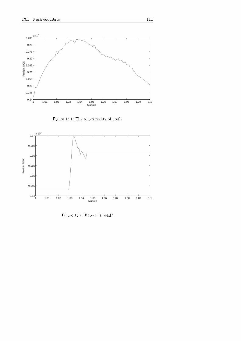
13.1 Nash equilibria 111
1 1.01 1.02 1.03 1.04 1.05 1.06 1.07 1.08 1.09 1.19.24
9.245
9.25
9.255
9.26
9.265
9.27
9.275
9.28
9.285x 10
5
Markup
Pro
fit in
NO
K
Figure 13.1: The rough reality of pro�t
1 1.01 1.02 1.03 1.04 1.05 1.06 1.07 1.08 1.09 1.19.14
9.145
9.15
9.155
9.16
9.165
9.17x 10
5
Markup
Pro
fit in
NO
K
Figure 13.2: Batman's head?

112 Chapter 13. Search algorithms
5 10 15 20 251
1.01
1.02
1.03
1.04
1.05
1.06
1.07
1.08
1.09
1.1
Iterations
Mar
kup
E2ElsamStatkraftVattenfallSydkraftFortrumEon
Figure 13.3: Suggested markup of production cost
0 5 10 15 20 251
2
3
4
5
6
7
8
9
10x 10
5
Iterations
Pro
fit o
f pla
yers
in N
OK
E2ElsamStatkraftVattenfallSydkraftFortrumEon
Figure 13.4: Pro�t of each player
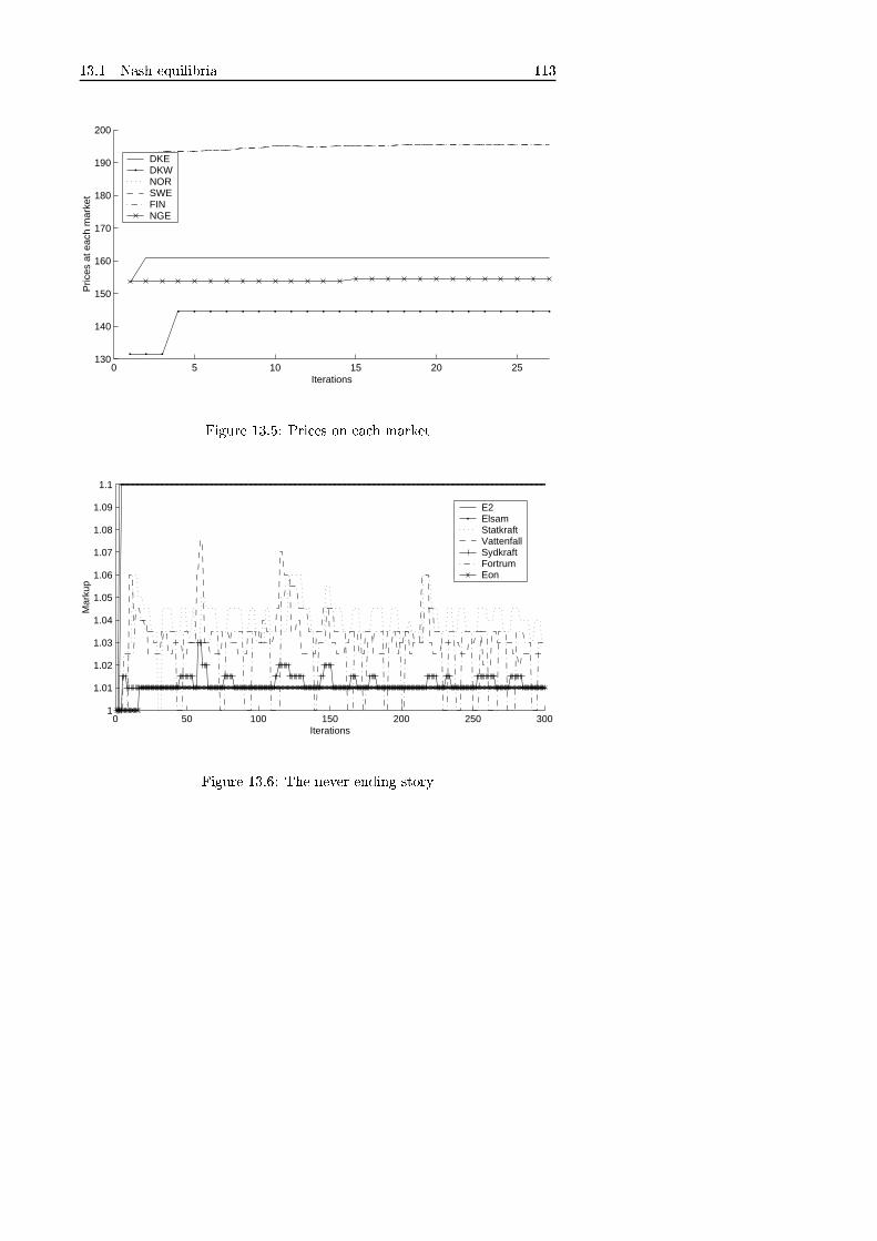
13.1 Nash equilibria 113
0 5 10 15 20 25130
140
150
160
170
180
190
200
Iterations
Pric
es a
t eac
h m
arke
t
DKEDKWNORSWEFINNGE
Figure 13.5: Prices on each market
0 50 100 150 200 250 3001
1.01
1.02
1.03
1.04
1.05
1.06
1.07
1.08
1.09
1.1
Iterations
Mar
kup
E2ElsamStatkraftVattenfallSydkraftFortrumEon
Figure 13.6: The never ending story

114 Chapter 13. Search algorithms
player B. Player A then responds with strategy A1 and the circle goes onand on.
More interesting is to view yet another run, with the same data, as shownin �gures 13.7 to 13.9. Here the algorithm terminates after ca. 90 iterationswith a slightly di�erent Nash equilibrium than in �gure 13.3. In additionto showing that more than one Nash equilibrium can be found, there wasa solution in the 43rd iteration, which was Pareto optimal to all foundNash equilibria and with considerable more pro�t for the northern players.Regrettably, bearing in mind the �nal equilibrium, Fortum, in this example,could increase their pro�t by a little underbidding, starting a downwardprice spiral and ending with each of the northern players acquiring onlyca. 1/3 of the market power pro�t, they could have earned. If Fortumactually had complete information of all bids, production cost and markupsof the other players, would they not have stopped there? Even without anycooperation with the other players, it would have been wise for Fortum tostop there. For producers, Pareto outshine Nash just as monopoly outshinesoligopoly.
0 10 20 30 40 50 60 70 801
1.01
1.02
1.03
1.04
1.05
1.06
1.07
1.08
1.09
1.1
Iterations
Mar
kup
E2ElsamStatkraftVattenfallSydkraftFortrumEon
Figure 13.7: The Finnish gambit
The Tuesday data produced rather boring results. After few iterations, thesame Nash equilibrium was always found, in which all markups are raised

13.1 Nash equilibria 115
0 10 20 30 40 50 60 70 800
1
2
3
4
5
6
7
8x 10
4
Iterations
Cha
nge
in p
rofit
in N
OK
E2ElsamStatkraftVattenfallSydkraftFortrumEon
Figure 13.8: Mountain of money?
0 10 20 30 40 50 60 70 80130
140
150
160
170
180
190
200
210
Iterations
Pric
es a
t eac
h m
arke
t in
NO
K
DKEDKWNORSWEFINNGE
Figure 13.9: The �nal price to pay for the competition

116 Chapter 13. Search algorithms
close to maximum, resulting in higher market prices on all markets. Figure13.10 demonstrates the results.
0 2 4 6 8 10 12 14 16 18 20 221
1.01
1.02
1.03
1.04
1.05
1.06
1.07
1.08
1.09
1.1
Iterations
Mar
kup
E2ElsamStatkraftVattenfallSydkraftFortrumEon
Figure 13.10: Iterated markup on Tuesday
13.2 Pareto optimality
A situation involving a Pareto optimality, or at least a more Pareto e�cientsolution than the `natural' Nash equilibrium, would indicate that not only ismarket power being used, but cooperation, either active or inactive, is alsotaking place between the players. This may produce considerably higherprices than the oligopolistic Nash equilibria, as monopolistic pro�t can begained from a more �restrained� competition.
In order to search for Pareto optimality, only slight modi�cations need tobe done to the search methods for the Nash equilibria.
1. Randomly select a player on a market where he operates.2. If the price on the market has not changed since the last time, that
player was selected on that market, remove him temporarily from theplayer pool and go to step 1.
13.2 Pareto optimality 117
3. Add di�erent markups to the selected player's bids, sort the supplycurve, and calculate his pro�t and prices on all markets.
4. Select the best markup.5. Remove the player from the pool and return all other players who
operate on markets where market price has changed, to the pool.6. If no player is left in the pool or after certain number of iterations,
terminate the process.7. Otherwise repeat from step 1.
The question remaining is, what the best markup would be, as mentionedin step 4.
As there can be quite a large number of Pareto optimal solutions for eachNash equilibrium, some, at least those with local maximums, can easily befound. Therefore, one will have to specify which attributes of the Paretooptimal solution one seeks.
A Pareto optimal solution must be fair to the players, although certainlynot to their customers, thus preventing a player, who would have wanteda more pro�table solution for himself, from seeking another solution. Asmost Pareto optimal solutions are not Nash equilibria, the temptation todo so may be great, especially if the player in question has reasons to expecta more pro�table solution around the corner.
I considered and tried out three methods for �nding Pareto optimal so-lutions from di�erent starting points, using the same approach as in thesearch for Nash equilibria:
1. The strategy chosen is the one that maximizes the pro�t of the currentplayer, while being more Pareto e�cient than the last solution.
2. The strategy chosen is the one which maximizes the total pro�t of allplayers, while being more Pareto e�cient than the last solution.
3. The strategy chosen maximizes the total pro�t of all players. This isrepeated until no better solution can be found. Then the last solutionis checked to see whether it is more Pareto e�cient than any known�natural� Nash equilibria.
When maximizing the total pro�t and subsequently comparing the resultto the 0 markup, both the Tuesday and Monday data gave the maximummarkup as the most pro�table for all players. The change from the Tues-day data was that Sydkraft was now using 10% markup instead of 9%,causing their pro�t to fall while the pro�t of the other northern players

118 Chapter 13. Search algorithms
increased more than Sydkraft's loss. The Monday data caused the pro�tof the northern players to increase dramatically and presented all playerswith the same pro�t as or more pro�t than any Nash equilibrium found.By comparing �gures 13.8 and 13.11 it can be seen that even the pro�tpeak discussed previously is dwarfed by the pro�t the northern players canattain.
0 2 4 6 8 10 12 14 16 18 200
2
4
6
8
10
12
14x 10
4
Iterations
Cha
nge
in p
rofit
in N
OK
E2ElsamStatkraftVattenfallSydkraftFortrumEon
Figure 13.11: Pareto on Tuesday
However, as can be seen in �gures 13.12 and 13.13, the newly acquired pro�tis not a Nash equilibrium as `greedy' Fortum (again) makes a short termpro�t by dropping the price in Sweden. The good Pareto optimal solutionbecomes the victim of competition which ends in a Nash equilibrium withfar less of a pro�t for the northern players.
13.3 Simulating annealing
Simulated annealing (SA) is a generalization of a Monte Carlo method forexamining the equations of state and frozen states of n-body systems.[29]The concept is based on the way in which liquids freeze or metals recrys-

13.3 Simulating annealing 119
0 10 20 30 40 50 601
1.01
1.02
1.03
1.04
1.05
1.06
1.07
1.08
1.09
1.1
Iterations
Mar
kup
E2ElsamStatkraftVattenfallSydkraftFortrumEon
Figure 13.12: A new Finnish gambit
0 10 20 30 40 50 60−12
−10
−8
−6
−4
−2
0
2x 10
4
Iterations
Cha
nge
in p
rofit
in N
OK
E2ElsamStatkraftVattenfallSydkraftFortrumEon
Figure 13.13: All is lost

120 Chapter 13. Search algorithms
talize in the process of annealing. In an annealing process a melt, initiallydisordered and at a high temperature, is slowly cooled so that the systemat any time is approximately in thermodynamic equilibria. As cooling pro-ceeds, the system becomes more ordered and approaches a �frozen� groundstate at T=0. Hence the process can be thought of as an adiabatic ap-proach to the lowest power state. If the initial temperature of the systemis too low or cooling is not done su�ciently slowly, the system may be-come quenched, forming defects or freezing out in metastable states (i.e.trapped in a local minimum energy state). The original Metropolis schemewas that an initial state of a thermodynamic system was chosen at energyE and temperature T, holding T constant, the initial con�guration is per-turbed and the change in energy dE is computed. If the change in energyis negative the new con�guration is accepted. If the change in energy ispositive it is accepted with a probability given by the Boltzmann factorexp -(dE/T). This process is then repeated for a su�cient number of timesto give good sampling statistics for the current temperature, and then thetemperature is decremented and the entire process repeated until a frozenstate is achieved at T=0.
By analogy, the generalization of this Monte Carlo approach to combinato-rial problems is straight forward.[30][31] The current state of the thermo-dynamic system is analogous to the current solution of the combinatorialproblem, the energy equation for the thermodynamic system is analogousto the objective function, and the ground state is analogous to the globalminimum. The major di�culty (art) in implementing the algorithm is thatthere is no obvious analogy of the temperature T with respect to a freeparameter in the combinatorial problem. Furthermore, avoidance of en-trainment in local minimums (quenching) is dependent on the �annealingschedule�, the choice of initial temperature, how many iterations are per-formed at each temperature, and how much the temperature is decrementedat each step as cooling proceeds.[28]
13.3.1 Application of simulated annealing to �nd Nash
equilibria
SA is a powerful optimization heuristic algorithm. In one of my programs,I gave each players opportunities to sometimes select a di�erent markupthan the optimal one. However, instead of using SA, I found more e�cientto randomly select di�erent starting points and walk the `straight' way into

13.4 Longer periods 121
some mixed or pure strategy Nash equilibrium. This was partially because,there often is no way to tell whether one Nash equilibrium is `better' thananother. Hence, the main bene�ts of SA, �nding global maximums, werenot exploited by its application for the Nash equilibria search.
13.3.2 Application of simulated annealing to �nd
Pareto optimality
I also used SA to search for Pareto optimal solutions, but later discoveredthe futility of such a search as the maximum markup was usually found tobe the `best' Pareto optimal solution.
Therefore, the use of SA did not contribute very much to the searches,although it may be practical under certain circumstances.
13.4 Longer periods
In the previous sections I have discussed methods for �nding Nash equilibriafor a single hour. However, as discussed in section 10.6.1, changing theprice strategy to meet hourly prospects is almost impossible. Players wouldtherefore have to �nd longer periods, on which to base their strategy.
13.4.1 Cycles
A strategy must be based on a kind of cycle which is repeated. The smallerthe cycle is, more pro�t can be gained as the strategy would be tailored toa short period. However, small cycles also require a �ner control of prices,which can be di�cult to maintain due to market surveillance. Longer cyclesare therefore easier to maintain but will not �t so well to each hour of thecycle. It is also more di�cult to calculate the best strategy for longerperiods as more data must be processed.
Days form a cycle as consumption is less during the day than the night.However, every week has a weekend with a considerably di�erentdemand, which would require changes to be made every week, anobviously impractical endeavor.

122 Chapter 13. Search algorithms
Weeks form a whole cycle with �ve high demand working days and twolow demand days at the weekend. However, weekly cycles do notcover seasonal changes in demand, which means that changes mustbe made to the strategy in the course the year.
Years form a cycle with full seasonal changes. Years should only di�erfrom each other as being either very cold or very warm and eithervery wet or very dry.
Longer weather periods due to climate changes or special weather phe-nomenona like El Nino and global warming, can form a cycle. It isprobably rather impractical to build a strategy based on such a longand unpredictable periods.
Weeks may be the most convenient size of cycle, as small changes in pricestrategies might trickle through with new seasons. In the following sectionsI will focus on weekly cycles.
13.4.2 Weeks
To �nd the optimal strategy for a week, one must �nd a strategy thatweighs �ve working days strategies with two weekend days strategies. Thedata from Eltra does form a single week, actually with di�erent a supplyfunction for each hour, with the wind power being the main source ofdeviation. The Monday and Tuesday, to which I have referred in severalprevious examples, were in fact fairly windy days, with quieter days tofollow.
However, it takes much more computer power to optimize a strategy basedon a whole week as opposed to a single hour. There are 168 (7 × 24)hours in a single week, which is the factor of increased computer time andmemory usage needed in comparison with hourly calculations.
13.4.3 Nash and Pareto
I made some modi�cations to the search algorithms I used to �nd hourlyNash equilibria and Pareto optimal solutions, to include the total pro�tcalculations for each markup for the whole week.
In order to decrease computation time, I reduced the number of strategiesavailable for each player by increasing the step length between available
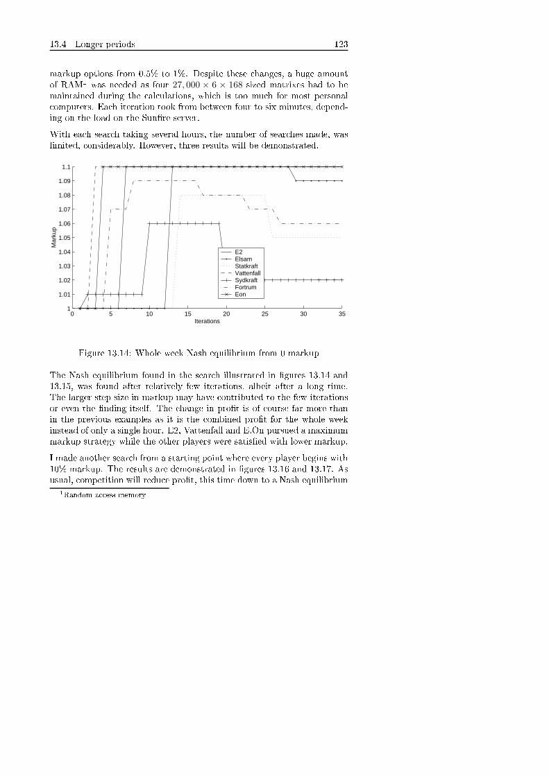
13.4 Longer periods 123
markup options from 0.5% to 1%. Despite these changes, a huge amountof RAM1 was needed as four 27, 000 × 6 × 168 sized matrixes had to bemaintained during the calculations, which is too much for most personalcomputers. Each iteration took from between four to six minutes, depend-ing on the load on the Sun�re server.
With each search taking several hours, the number of searches made, waslimited, considerably. However, three results will be demonstrated.
0 5 10 15 20 25 30 351
1.01
1.02
1.03
1.04
1.05
1.06
1.07
1.08
1.09
1.1
Iterations
Mar
kup
E2ElsamStatkraftVattenfallSydkraftFortrumEon
Figure 13.14: Whole week Nash equilibrium from 0 markup
The Nash equilibrium found in the search illustrated in �gures 13.14 and13.15, was found after relatively few iterations, albeit after a long time.The larger step size in markup may have contributed to the few iterationsor even the �nding itself. The change in pro�t is of course far more thanin the previous examples as it is the combined pro�t for the whole weekinstead of only a single hour. E2, Vattenfall and E.On pursued a maximummarkup strategy while the other players were satis�ed with lower markup.
I made another search from a starting point where every player begins with10% markup. The results are demonstrated in �gures 13.16 and 13.17. Asusual, competition will reduce pro�t, this time down to a Nash equilibrium
1Random access memory

124 Chapter 13. Search algorithms
0 5 10 15 20 25 30 350
2
4
6
8
10
12
14
16x 10
6
Iterations
Cha
nge
in p
rofit
in N
OK
E2ElsamStatkraftVattenfallSydkraftFortrumEon
Figure 13.15: Pro�t change for weekly Nash equilibrium search
0 5 10 15 20 251
1.01
1.02
1.03
1.04
1.05
1.06
1.07
1.08
1.09
1.1
Iterations
Mar
kup
E2ElsamStatkraftVattenfallSydkraftFortrumEon
Figure 13.16: Whole week Nash equilibrium from 10% markup

13.5 Comparison to actual prices 125
0 5 10 15 20 25−10
−8
−6
−4
−2
0
2x 10
6
Iterations
Cha
nge
in p
rofit
in N
OK
E2ElsamStatkraftVattenfallSydkraftFortrumEon
Figure 13.17: Dwindling pro�t
found very close to the equilibrium from the earlier search when comingfrom the opposite direction.
A search for Pareto optimality is illustrated in �gure 13.18. The searchmaximized the combined pro�t of all players, starting at 0% markup. Asexpected, the solution is found where each player uses maximum markup.
Statkraft, Vattenfall, and Fortum are the only players to bene�t to anyextent from the Pareto optimal solution, compared to the Nash equilibriafound in this section, as most of the other players were using maximummarkup anyway. Therefore, the support of other players for any form ofcooperation may be minimal.
13.5 Comparison to actual prices
In this section I will compare some of the prices found to the actual pricesduring the week from Monday to Sunday, February 10-16, 2003. Priceswithout markup, the Nash equilibrium found in the last section, the Pareto

126 Chapter 13. Search algorithms
0 2 4 6 8 10 12 14 16 18 20−5
0
5
10
15
20x 10
6
Iterations
Cha
nge
in p
rofit
in N
OK
E2ElsamStatkraftVattenfallSydkraftFortrumEon
Figure 13.18: The merit of cooperation
optimal solution with 10% markup and the actual prices that week, arecompared.
Figure 13.19 shows the prices in western Denmark for this period. As theNash markup was 9% there is almost no di�erence between the Nash andPareto solutions. However, the actual prices are far higher than any of theother modelled prices. There is, however, a correlation between the actualprice and other prices during the working days, but the demand during theweekend seems to have been underrated. The actual price appears to bebetween NOK 100 and 200 above the modelled prices.
Figure 13.20 illustrates the prices in Sweden. Here there is a larger di�er-ence between the modelled prices and as in Denmark, the actual prices arefar higher. There is also a correlation between the actual prices and themodelled prices during working days, but the weekend demand appears yetagain to have been underrated.
Finally, �gure 13.21 shows the prices in Germany. Although the actualprices are far closer to the modelled prices, especially during the night andat weekends, the price di�erence during peak demand is considerable.

13.5 Comparison to actual prices 127
0 20 40 60 80 100 120 140 160100
150
200
250
300
350
400
Hours
Pric
e in
NO
K
Nash equilibriaWithout market powerPareto optimalityActual price
Figure 13.19: Prices in western Denmark
0 20 40 60 80 100 120 140 160100
150
200
250
300
350
400
Hours
Pric
e in
NO
K
Nash equilibriaWithout market powerPareto optimalityActual price
Figure 13.20: Prices in Sweden

128 Chapter 13. Search algorithms
0 20 40 60 80 100 120 140 160100
150
200
250
300
350
400
Hours
Pric
e in
NO
K
Nash equilibriaWithout market powerPareto optimalityActual price
Figure 13.21: Prices in Germany
All three markets are characterized by the same shortcomings in the mod-elling, as opposed to the actual prices.
• There is too small price di�erence during the day and the night• Prices are too �at during the weekend• Prices are too low
It is worth taking into account that prices were considerably higher duringthis period in early 2003, than they had been in the previous years. Thisis demonstrated in �gure 13.22 which shows the average daily prices fromJuly 1999 to July 2003. Although it is clear that the model and data fail tosimulate the actual price level during this exceptional time, it would havebeen more accurate had it been for February 2002 instead of 2003.
The model does not accurately re�ect the actual prices for the period inquestion. The reasons could be:
• Demand was underestimated• Changes in demand during the days were underestimated• Actual unpredicted outages may not have been taken into considera-tion in the data

13.5 Comparison to actual prices 129
2000 2001 2002 2003
100
200
300
400
500
600
700
800
Time
Ave
rage
dai
ly p
rices
February 2003
Figure 13.22: Average daily system price on the Nord Pool spot market
• The markup that players use is far greater than the 10% used in themodels
• The production cost given in the data may be too low• The water reservoir prospects given in the data may have been toooptimistic
• Market power was being exercised on a considerably greater scalethan expected
Unless a closer match between the model and actual prices can be made,using the model and the data to build real price strategies may prove fu-tile. The data is, however, a platform, which should help in understandingthe market and building models which may help either to detect marketpower or to use it. One must always take into consideration that priceswere unusually high during February 2003 and models are usually built for`normal' circumstances and thus do not handle `extreme' situations well.The data and model might therefore have performed better in simulatingactual prices at another time.

130 Chapter 13. Search algorithms
13.6 Searches and results
In this chapter, I have searched for Nash equilibria and Pareto optimalsolutions. Although some were found, they must be taken with reservationas the application of this method to the real market may be quite di�cult.
13.6.1 To be or not to be
The Nash equilibria found were usually unstable as pure strategy equilibriaoften became mixed strategy equilibria when the step size was decreased.Therefore, in a way they never existed but were only the result of an ap-proximation of discreet strategies.
The de�nition of the only `true' Nash equilibria has to be when no possiblestrategy of any player will increase that player's pro�t. And strategies be-tween the discreet steps, must be considered possible strategies. Therefore,many of the pure strategy Nash equilibria found were not in reality Nashequilibria.
13.6.2 Incomplete information
To be able to �nd a Nash equilibrium, players must be able to select theiroptimal strategy. For the selection, a player must either know the exactdemand and bids of other players or be able to determine his best strategyby stochastic or systematic search (trial and error).
The problem is that neither approach is easily accessible. The necessaryinformation is not publicly available and guessing, based on the systemprice, volume traded, international transmission and ones own bids, willleave a lot of uncertainties.
Although, if partially accepted, the highest accepted bid would be at themarket price, no information would be available on how large a part of itwas accepted or the price and volume of the lowest unaccepted bid or secondhighest accepted bid. Had the highest accepted bid been fully accepted, ofwhich there is no way of telling, information on neither the volume nor theprice of that bid would be available.
This makes the �ndings in chapter 11 rather unhelpful, as they require theknowledge of not only other bids around the market price, but also their

13.6 Searches and results 131
production cost, in order to select the optimal price strategy and to makethe correct underbidding.
Regarding the stochastic or systematic search, for the detection of the op-timal strategy, it requires the ability to change prices frequently in orderto check the new strategies. However, this is not possible as �changes inmarket behavior that is not motivated by serious commercial or technicalcircumstances must not occur.� Therefore, such a search would take sometime, and during that time, di�erent circumstances may have arisen onthe market, such as di�erent temperature, season etc. This may make theeventual comparison of strategies obsolete.
13.6.3 Unpredictability
To add to the di�culties, unpredictability plays a part in making the opti-mization of a price strategy more di�cult as the market and market pricescan be constantly shifting. The following factors will add to the variationof market prices:
• Wind power and winds• Water reservoir levels, rain and temperature• Temperature• Outages of power plants and transmission lines• Opening up of new installations or closing down of old ones• Changes in other players' strategies
13.6.4 Enlightenment
If we assume that all the necessary information was available to a player,he would still have di�culties in deciding his optimal strategy. As demon-strated in section 13.2, a short term e�ort to increase pro�t may sometimesalmost certainly result in a considerably lower market price with less pro�tfor all players. Such a strategy would probably not be selected by a playerpossessing all information, including information on how other players willmost likely respond. Can such a shortsighted strategy in that case be con-sidered pro�table, although it may be so for a very short period?
This takes us to the de�nition of Nash equilibrium. Should the Nash equi-librium be de�ned for only a short term pro�t or for a long term pro�t,

132 Chapter 13. Search algorithms
taking into account the expected response of other players? Is a combi-nation of Pareto and Nash more likely to be an `equilibrium' than a basicNash equilibrium?
13.6.5 Market power and Nash equilibria
To be able to �nd Nash equilibria, some information must be available.The information alone would be enough to decide whether market powerwas taking place, as any price above the production cost of the last unitproduced is, according to de�nition, a result of market power.
Therefore, as it is not only di�cult �nd Nash equilibria on the Nord Pool'sspot market, but also de�ning it, search for Nash equilibrium cannot beconsidered an e�ective tool for market power detection.

Part V
Conclusions
133


135
Chapter 14
Conclusions
14.1 Overview
In this thesis, I have described the Scandinavian electricity power mar-ket, the forming of Nord Pool and the characteristics of the market andelectricity markets in general.
I have discussed some of the elements of the game theory that can beapplied to the power market, in order to explain the behavior, strategiesand options of the electricity producers, as well as discussing the di�erentforms of competition and cooperation that can exist between them.
Furthermore, I have addressed some of the possible forms of market power,from changing prices or withholding production, to wrong predictions andblocking grid lines, and the possible bene�ts of each approach for di�erentproducers under di�erent circumstances. I also discussed who will gain andwho will lose by the use of market power and what can be done to detectit.
Finally I performed an extensive search for Nash equilibria and Paretooptimal solutions, which can both be clear indications of market power.

136 Chapter 14. Conclusions
14.2 Results
14.2.1 Market power
There are quite a few ways to exercise market power and changing pricesis only one of them.
Market power is when prices are higher than the actual production cost.Indeed, if production cost, production and demand is known, prices withoutthe use of market power can easily be calculated. Any price above that priceindicates that market power is being used, whether that price be a Nashequilibrium or not.
Market power also carries a disadvantage for its user and the main bene�-ciaries will often be competitors, who do not have to pay the price of lesssales. Market power also carries the risk of disclosure, which may have se-rious consequences. Therefore, it is not certain that the exercise of marketpower is always justi�able for producers.
14.2.2 Nash equilibrium
The search for pure strategy Nash equilibria showed the weakness of thatapproach and the instability of the equilibria found. Pure strategy Nashequilibria disappear with di�erent sets of strategies and other Nash equi-libria may be formed.
14.2.3 Pareto optimality
With a very few players, mindless competition will hurt the players withlow prices, to the customers' delight. Especially when the Nash equilibriaare as unstable as mentioned above, �nding a more favorable solution forall players, than any Nash equilibrium, would be fairly possible.
14.2.4 Parameters
Both Nash equilibrium and Pareto optimal solutions are greatly dependanton the parameters being used. In addition to the production cost and

14.3 Conclusions 137
production quantity, is is necessary to know the maximum markup andwhether all players are in fact using market power. Any deviation mayresult in considerably di�erent solution.
As demonstrated in section 13.5, the modelled prices did not accuratelyre�ect the actual prices for the period in question. While a more accuratesimulation of the prices cannot be made, based on available data, searchingfor Nash equilibria will not give useful �ndings.
Wind, temperature, rain, outages etc., add to the instability of possiblesolutions.
14.2.5 Incomplete information
Given the di�culty involving �nding a Nash equilibrium, when knowingevery move of the other players, �nding an equilibrium, not knowing any-thing except from own bids, prices on each market, international transmis-sion and total sales, is far more di�cult. A players cannot assume muchabout all the bids he must underbid to make more sales nor how much hecan increase prices and not be replaced by other players. And for a playerto know whether his own strategy is the optimal one, can be di�cult whenprices can only be changed at a slow rate and di�erent circumstances mayhave arisen later, making the comparison obsolete.
14.3 Conclusions
My �ndings are that although applying elements of the game theory tothe Scandinavian electricity power market may help us to understand thebehavior and functions of the market, searching for Nash equilibria doesnot, with current information, contribute much to the detection of marketpower. Less `sophisticated' approaches, as described in section 10.7, willprobably produce more useful results.
14.4 Further studies
Further studies may include more stochastic approaches in �nding optimalstrategies for players, as the mean or average situation, may not necessarilyyield the best solution.

138 Chapter 14. Conclusions

Part VI
Appendices
139

141
Appendix A
Elspot areas and bidding
information
A.1 ELSPOT AREAS AND BIDDING INFOR-
MATION
1.1 Elspot areas are those areas, into which the Electricity Exchange Areais divided in order to remedy capacity constraints, if any, in the grid. Theborders of the Norwegian elspot areas may vary. For the remaining of theElectricity Exchange Area the borders are �rm.
1.2 The System Operators determine how the elspot areas are to be di-vided and the transmission capacity, i.e. the maximum power �ow allowedbetween the elspot areas.
1.3 For Participants who bid in Norwegian elspot areas the System Oper-ator in Norway may, in accordance with NVE's �Guidelines for the systemoperator�, de�ne a elspot area as a monopoly area if a producer or consumerin the relevant area are so dominant that normal market mechanisms donot work. On such occasions, Bids related to the relevant area are totaledwith Bids related to the most suitable neighboring area so that the areashave a common price.
1.4 Every Thursday before 12:00 noon NPS shall inform the Participantsof the price range within which Bidding may be made during the week to

142 Appendix A. Elspot areas and bidding information
come; of the elspot areas for which separate Bidding are to be given; andof the de�nition of the elspot area borders. The price range is the upperand lower price for which Bidding may be made. The price range can bechanged from day to day when required.
A.2 BIDDING FOR PURCHASE AND SALE
2.1 Bidding may only take place in areas where the relevant Participantundertakes production, consumption or is party to contracts relating tophysical delivery or purchase.
2.2 Hourly Bid is the Participant's speci�cation of purchase and sale perhour. In the hourly Bid the Participant shall submit a set of price/quantityspeci�cations for each purchase and/or sale he wishes to make, divided intohours and elspot areas.
2.3 Block Bid is the Participant's speci�cation of purchase and sale for anin advance determined number of hours. In the block Bid, the Participantshall submit average price and average volume per block. NPS determineswhich hours are to be included in each block.
2.4 Flexible hourly Bid is the Participant's speci�cation of possible addi-tional sales in the hour with the highest price, with received hourly andblock Bids as the basis for calculation. The Participant speci�es price limitand volume for a �exible hourly bid in a speci�c elspot area.
2.5 Bidding from Trading- and Clearing Representatives shall be speci�edfor each Clearing Customer and for the Trading- and Clearing Representa-tive's own Bidding.
2.6 The Participant shall use the Bidding to achieve energy balance ineach elspot area. In order to control that this is done, NPS may requiredocumentation for the Participant's basis for Bidding. This document is atranslation and does not constitute a legally binding document 20
2.7 The Participant may submit hourly Bids, block Bids or �exible hourlyBids for one or several days within the period for which elspot areas havebeen determined. An hourly Bid and a �exible hourly Bid can be valid inone or several days. A block Bid is valid in one block only. New Bids maybe made for periods for which a Bid has already been made, provided that2.1 above is observed. It is the hourly Bid last received that counts.

A.3 PRICE SETTING 143
2.8 By no later than 12:00 noon each day the Participant has to submit hisBidding relating to the next day.
2.9 Prices are to be quoted in a currency approved by NPS. The correctnumber of decimals to be quoted in each currency is determined by NPS.The Bidding may quote the number of MWh with up to one decimal. TheParticipants must make their Biddings for purchase and sale within therelevant price range. If NPS changes the price range in accordance withArticle 1.4, The Participants must submit new Bidding for the remainingdays of the week.
2.10 Bidding shall be made on NPS' standard bidding form and transmittedto NPS per electronic communication as speci�ed by NPS. Fax may beused when approved by NPS. The Bidding form must provide completeinformation in order to be valid. Invalid or faulty Bidding will be rejected.In case of rejection, the price report received by the Participant from NPSwill declare that no contract is concluded.
2.11 NPS may in exceptional and isolated situations claim that the Partic-ipants make Biddings for several following 24-hour periods. NPS shall insuch situations give notice of the situation to the Participants at the lat-est one week in advance and simultaneously inform of how many 24 hourperiods which must be included in the Bidding.
A.3 PRICE SETTING
3.1 The price/quantity speci�cations of the Bids will be regarded as pointson a bidding curve created by drawing straight lines between the points.
3.2 The block Bid is granted the tender if the criteria below are met. Ablock Bid (sell) is granted a tender if the average price for the hours issimilar to or higher than bidden price. A block Bid (buy) will be granteda tender if the average price for the hours is similar to or below biddenprice. In addition, the submitted volume must be ful�lled. The selectionis based on the following criteria: 1. The di�erence between submittedprice and average area price. This means that the block bid which has thelargest di�erence between submitted price and average area price will beexcluded �rst. This document is a translation and does not constitute alegally binding document 21 2. Energy, which means volume multipliedwith the number of hours in the block. If the di�erence between submitted

144 Appendix A. Elspot areas and bidding information
price and area price is equal, then the block bid or the combination of theblock bids that gives the largest turnover will be given priority. 3. Time ofstoring. If two block bids or combinations of block bids are similar, thenthe bid which is �rst stored in NPS price setting database will be givenpriority.
3.3 A �exible hourly Bid may be granted the tender if the price- and volumecriteria are met. NPS may decide that a �exible hour Bidding shall not begranted the tender if it alters the status for tenders of the block Bids. NPS'priorities of �exible hourly Bids shall be based on the following criteria: 1.Price; being the di�erence between the price of the �exible hourly Bid andthe area price. 2. The time of the storing in the database. Item 3.2 (3)applies correspondingly.
3.4 Based upon Biddings received NPS �rst calculates a system price. Thesystem price is the price in those elspot areas that at the relevant time areincluded in the system price calculation. The system price calculation isdone by aggregating all Bids in one buy curve and one sell curve withoutconsidering potential capacity constraints between the relevant areas. Thepoint of intersection between the two curves establishes the system price.
3.5 If the power �ow between two or more elspot areas exceeds the trans-mission capacity, two or more area prices will be calculated.
3.6 If situations occur where a point of intersection between the buy curveand the sell curve is not achieved, NPS may reduce Bids on a pro rata basisuntil an intersection point is achieved.
3.7 Any imbalance between total purchase and total sale caused by therounding o� of quantity for each Participant when accurately calculatingthe price will be distributed within each elspot area (system price or areaprice).
3.8 All prices are calculated in NOK and are converted to other currencies.
A.4 REPORTS OF PURCHASE AND SALE
4.1 When the price has been calculated NPS informs the Participant ofits calculated purchase/sale in a price report which shall be submitted tothe Participant before 13.30 hours the day preceding the day for whichthe price is given. The price report speci�es the price and quantity for

A.4 REPORTS OF PURCHASE AND SALE 145
each elspot area for which the Participant has bidden. Price reports tothe Trading- and Clearing Representatives are speci�ed for each ClearingCustomer and for the Trading- and Clearing Representative's own Trading.If transmission of the price report is delayed, notice shall be given.
4.2 If the Participant wants to claim an error in NPS' handling of a Bid,NPS shall be noti�ed before 14:00 hours on the same day. The Trading- andClearing Representatives claim errors on behalf of Clearing Customers. TheParticipant shall if relevant, receive a new price report before 14:30 hours.If transmission of the price report is delayed, the Participant is granted 30minutes to submit notice of error, calculated from when the price report istransmitted from NPS, and correspondingly NPS has one hour to resenda corrected price report, if relevant. Upon expiry of the notice period theprice report transmitted will be regarded as a contractual obligation forthe quantities speci�ed in the price report.
4.3 In situations described in 2.11, NPS will, if needed, determine separaterules for price reports and deadlines for submitting notice of errors.

146 Appendix A. Elspot areas and bidding information

147
Appendix B
Matlab codes
In the following section, a few of the most important types of the matlabalgorithms I wrote, can be found.
B.1 Price calculations
function [C,m,pris]=nordpoolshort(M,KAP,z)
% M is matrix made of 12 vectors where the first 6 give the price
% of the supply function and the latter 6 the demand function for
% each of the 6 markets.
% KAP(i,j) gives the maximum transmission capacities from market
% i to market j.
% z=1000; %The starting number of unit transfer between markets.
he=0; %Counter
zz=5; %The factor of how z is decreased
log1=0; %Varible which decides when to stop the main loop
[nn,antakt]=size(M);
%Defines length and breadth of the main information matrix M
antakt=antakt/2; %How many markets there are

148 Appendix B. Matlab codes
C=zeros(antakt,antakt);
%C(i,j) is the current export from market i to market j
pd(1:antakt)=0; %Netto import to a market
for k=1:antakt %Initial price calculation before exports
[pkk, mk] = min( abs(M(:,k)-M(:,antakt+k)) );
%Finds where the difference between supply and demand is
%least for each market
m(k)=mk;
%Marks the current position of the current price in each market
pris(k)= M(m(k),antakt+k);
%Finds price in beginning before exports and imports
end
changed=[1:antakt];
% Defines which markets need to be calculated
while (log1 ~=1)
%The main loop, will end when log1 becomes 1
he=he+1; %Counter
tpd=pd-z; %Moves forward or backward when export or import
if length(changed)==2
% After a normal transmission only the 2 relevant markets
% needs recalculations.
overf(:,changed(1))=1;
overf(changed(2),:)=1;
% Allows calculations of export from markets which exported in last
% iteration and import for markets which imported in last iteration
% Other calculations are unecessary as they have already been made
% The following lines find new prices for each market when receiving
% import or export. They only checks for new price in the area from
% last known price and up to + or - z (the transfer unit)
% in case of exporting or importing
B.1 Price calculations 149
r1=changed(2);
% r1 is the market which received import last iteration
[pkkn1, mkn1(r1)] = min( abs(M(-z+m(r1):m(r1),r1)-
M(pd(r1)+m(r1):pd(r1)+m(r1)+z,antakt+r1)) );
% New position for maret r1 when receiving import z
prisn1(r1)= M(pd(r1)+m(r1)+mkn1(r1)-1,antakt+r1);
% New for price for market r1 when receiving import z
r2=changed(1); % r2 is the market which received export last iteration
[pkkn2, mkn2(r2)] = min( abs(M(m(r2):m(r2)+z,r2)-
M(tpd(r2)+m(r2):tpd(r2)+m(r2)+z,antakt+r2)) );
% New position for market r2 when exporting z
prisn2(r2)= M(tpd(r2)+m(r2) +mkn2(r2)-1,antakt+r2);
% New price for market r2 when exporting z units
else
% When z has been changed, or in the beginning, export and import
% for all markets must be calculated
overf=ones(antakt,antakt); %Makes all calculations necessary
for r1=changed
% This loop does the same as in above, except all markets are checked
% for export and import, instead of only 1 for export and 1 for import.
[pkkn1, mkn1(r1)] = min( abs(M(-z+m(r1):m(r1),r1)
-M(pd(r1)+m(r1):pd(r1)+m(r1)+z,antakt+r1)) );
prisn1(r1)= M(pd(r1)+m(r1)+mkn1(r1)-1,antakt+r1);
r2=r1;
[pkkn2, mkn2(r2)] = min( abs(M(m(r2):m(r2)+z,r2)-
M(tpd(r2)+m(r2):tpd(r2)+m(r2)+z,antakt+r2)) );
prisn2(r2)= M(tpd(r2)+m(r2) +mkn2(r2)-1,antakt+r2);
end
end
overf = and(overf,(KAP >= C+z));

150 Appendix B. Matlab codes
% overf(i,j) is 1 when legal transmission is possible from market i to j.
% This marks all legal, when KAP >= C+z and necessary when overf<>0
% calculations
[oi,oj]=find(overf); % Vectors with the position of legal transmissions
if(oi) % If any legal transmission
for i=1:length(oi)
r1=oj(i);
r2=oi(i);
if pris(r1)>pris(r2) % Export is possible if the receiving country
% has higher price and there is enough capacity
overf(r2,r1)=(abs(prisn1(r1)-prisn2(r2))<= pris(r1)-pris(r2));
% But only if the price difference between markets becomes less
else
overf(r2,r1)=0; %If the price in exporting market is higher,
% export is illegal
end
end
end
if find(overf) %Checks wether there is any legal move
[s1, s2] = sort(pris); %s2 sorts the markets after the
% current price, the market with the highest price is last
im=antakt; %Varibles used to find best import
ex=1; % and export
while ~overf(:,s2(im))
% Finds the most expensive market which can receive import
im=im-1; % Checks for next market
end

B.1 Price calculations 151
j=s2(im); %j is that market
while ~overf(s2(ex),j)
% Finds the cheapest market which can export to market j
ex=ex+1; % Checks for next market
end
i=s2(ex); % i is that market
C(i,j) = C(i,j) + z;
% Energy of volume z is transferred from market i to market j
pd(j)=pd(j)+z; % Netto import for market j is increased
pd(i)=pd(i)-z; % Netto import for market i is decreased
mkn1(i)=z-mkn2(i)+2; % Position of import changes
m(i)=m(i)+mkn2(i)-1; % New positions of price
prisn1(i)=pris(i); % Old price become new export price
pris(i)= prisn2(i); % and new price is old export price.
mkn2(j)=z-mkn1(j)+2; % Position of export changes
m(j)=m(j)+mkn1(j)-1-z; % and new position found
prisn2(j)=pris(j); % Old price becomes new import price
pris(j)= prisn1(j); % Old import price becomes new price.
changed=[i,j];
% The market that have changes. What is necessary to calculate are
% new import price for j and export price for i other information are
% reused.
else % Well, if there was no legal export or import
if z>1
z=ceil(z/zz); % we will decrease the amount transferred

152 Appendix B. Matlab codes
changed=[1:antakt]; % and must calculate all markets with new z
else
log1=1; % unless z is already 1 and then we will end the main loop
end
% The following lines net out the transmission, if transmission from
% i to j and from j to i, the lesser transmission becomes 0 and the
% greater transmission the difference
CC=C';
[i,j]=find(and(C>CC,CC));
if i
for k=1:length(i)
C(i(k),j(k))=C(i(k),j(k))-C(j(k),i(k));
C(j(k),i(k))=0;
end
end
end
end % The end of the main loop

B.2 Data preperation 153
B.2 Data preperation
function [S,D, mpt,mpro]= hentmp3(uge,dag,time,tol)
% Function which takes the number of week, day and hour
% as well as the minimum unit.
tic
load eltra % Loads Etra's data including demand which is the demand data,
% timi, which is the time index for the supply data, and supplymp which
% which is the supply data, and supplier, which is the supplier index
% in the supply data.
q3=5000; %Highest price
m=6; %How many markets
vektor=find(and(timi(:,1)==uge, and(timi(:,2)==dag, timi(:,3)==time)));
sup1=supplymp(vektor,:);
% Finds the supply elements for the correct date
vektor=find(and(demand(:,1)==uge, and(demand(:,2)==dag,
demand(:,3)==time))); dem1=demand(vektor,4:end);
% Finds the demand elements for the correct date
%%%% Calculates new demand
vektor=[2:2:m*2];
dvol=dem1(:,vektor-1); % The volume
dpris=dem1(:,vektor); % and the price are found
mx=floor(max(max(dvol))/tol); %How many units in vector
nydem1=zeros(mx,m); % The new demand later
for i=1:m
% This loops interpolates the demand for each of the markets
% between the data points given by Eltra
[mest,hvar]=max(dvol(:,i));
dvec=interp1(dvol(1:hvar,i),dpris(1:hvar,i),[tol:tol:mest]');
nydem1(1:length(dvec),i)=dvec;

154 Appendix B. Matlab codes
end
%%%%%%% Calculates new supply
n=size(sup1); supplier=n(2)/2; offers=n(1); vektor=[2:2:n(2)];
svol=sup1(:,vektor-1); spris=sup1(:,vektor);
supply=[];
market=[]; %Which market
producer=[]; %Number of producer
pt=[]; %Producers team
counter=0; ;
%%% The following loops find each supplier, and interpolates his supply for
%%% all the markets as well as recording his ownership
for i=1:supplier
[mest,hvar]=max(svol(:,i));
if mest>0
svec=interp1q(svol(1:hvar,i),spris(1:hvar,i),[tol:tol:mest]');
ls=length(svec);
supply(counter+1:counter+ls,1)=svec;
producer(counter+1:counter+ls,1)=ones(ls,1)*i;
counter=counter+ls;
end
end
pt=team(producer); % Records faction ownership for each element in the supply
market=landn(producer); % Records on which markets each faction operates
%Sorts markets
msup=ones(mx,m)*q3;
%%% The following loop adds all the supply functions for all the producers
%%% togehter for each market, sorts it, and keeps record of the ownership
%%% and type of each plant.
for i=1:m
vektor=find(market==i);
l=length(vektor);
s=supply(vektor);
[q,si]=sort(s);
msup(1:l,i)=s(si);
mpro(1:l,i)=producer(vektor(si),:);

B.2 Data preperation 155
mpt(1:l,i)=pt(vektor(si),:);
end
[q,qq]=max(msup); q=max(qq)-1;
D=nydem1(1:q,:)*tol; % The demand matrix
S=msup(1:q,:)*tol; % The supply matrix

156 Appendix B. Matlab codes
B.3 Iterative search for Nash equilibrium
% This program randomly selects market, finds the best solution for
% that market and keeps that solution.
% This is version is with sepperate markup for subsidiaries in other markets
tic clear
tol=1; %Minimum unit in MWh
[M,D,pt,pd]= hentmp3(7,1,1,tol); %Gets data for week, day, hour and with
% minimum unit. M is supply, D is Demand, pt and pd are the ownership and
% power plant type of the supply.
init1 % Gets few text strings for the later plotting
toc tic
z=1000/tol; % Starting transfer between markets
KAP=KAP/tol; % The allowable maximium transfer between markets
ww=[1:0.001:1.1]; %Steps and scope of price changing
load eltra teammarket; %Load data about on which markets teams operate
[stm1 stm2]=size(teammarket);
M=[M;[5000*tol*ones(z,antakt)]];
D=[D;[zeros(z,antakt)]]; %Extends M to avert fails in Sweden
pt=[pt;[zeros(z,antakt)]];
MM=M; kk=0; toc tic kkk=0;
r=0;
other=0; %Which market is not to be tested.
lm=length(M);
[temp, lam]=max(M); %Actual length of each market
player=[2, 4, 8,10,9, 7, 6]; lp=length(player);
other=zeros(lp,1);
tvekt=[];
vektor=ones(stm2,lp);
tind=zeros(lm,lp,antakt); tindl=zeros(lp,antakt);
for i=1:lp
for j=1:antakt

B.3 Iterative search for Nash equilibrium 157
t=find(pt(1:lam(j),j)==player(i));
tindl(i,j)=length(t);
if(tindl(i,j))
tind(1:tindl(i,j),i,j)=t;
end
end
end
fpt=pt; oldprice=zeros(lp,antakt); price=ones(1,antakt);
%Fast
information(1,2,stm2)=0; income(1,lp)=0; cost(1,lp)=0;
while and(kkk<300,sum(other)<lp);
r=floor(rand*lp)+1;
while other(r);
r=floor(rand*lp)+1;
end
toc
tic
mm=player(r);
for tm=1:stm2
am=teammarket(mm,tm) %Active market
if am>0
if oldprice(r,am)==price(end,am)
other(r)=1;
else
kk=0;
kkk=kkk+1
if kkk==1
www=1;
else
www=ww;
end
for w=www;
kk=kk+1;
fvekt=find(fpt(1:lam(am),am)==mm);
MM(fvekt,am)=M(tind(1:tindl(r,am),r,am),am)*w;

158 Appendix B. Matlab codes
[MM(1:lam(am),am),f]=sort(MM(1:lam(am),am));
fpt(1:lam(am),am)=fpt(f,am);
%end
information(kk,:,tm)=[mm w];
[C,m(kk,:),pris(kk,:)]=nordpoolshort([MM,D],KAP,z);
%for i=1:lp
for i=r
for j=teammarket(player(i),
1:length(find(teammarket(player(i),:))))
salg=find(fpt(1:m(kk,j),j)==player(i));
lsalg(kk,i,j)=length(salg);
mincome(kk,i,j)=lsalg(kk,i,j)*pris(kk,j);
mcost(kk,i,j)=sum(M(tind(1:lsalg(kk,i,j),i,j),j));
end
income(kk,i)=sum(mincome(kk,i,:));
cost(kk,i)=sum(mcost(kk,i,:));
end
end
profit=income-cost;
[bb,best]=sort(profit(:,r));
vektor(tm,r)=information(best(end),2,tm)
fvekt=find(fpt(1:lam(am),am)==mm);
MM(fvekt,am)=M(tind(1:tindl(r,am),r,am),am)*vektor(tm,r);
[MM(1:lam(am),am),f]=sort(MM(1:lam(am),am));
fpt(1:lam(am),am)=fpt(f,am);
kk=best(end);
for i=1:lp
for j=teammarket(player(i),
1:length(find(teammarket(player(i),:))))

B.3 Iterative search for Nash equilibrium 159
salg=find(fpt(1:m(kk,j),j)==player(i));
lsalg(kk,i,j)=length(salg);
mincome(kk,i,j)=lsalg(kk,i,j)*pris(kk,j);
mcost(kk,i,j)=sum(M(tind(1:lsalg(kk,i,j),i,j),j));
end
income(kk,i)=sum(mincome(kk,i,:));
cost(kk,i)=sum(mcost(kk,i,:));
end
profit=income-cost;
price(kkk,:)=pris(best(end),:);
vek(kkk,:,: )=vektor(:,:)';
opt(kkk,:)=profit(best(end),:);
if opt(kkk,r)==opt(max(1,kkk-tm),r)
else
other=zeros(lp,1);
oldprice(r,am)=price(kkk,am);
end
other(r)=1;
end
end
end
end
figure hold for i=1:lp
plot(vek(:,i,1),texti3(i,1:3))
end legend(firmanavn(player,:),0) xlabel('Iterations');
ylabel('Markup');
v=axis;
v(4)=w;
v(2)=kkk;
axis(v);
figure hold for i=1:lp
plot(opt(:,i)-opt(1,i),texti3(i,1:3))
end legend(firmanavn(player,:),0) xlabel('Iterations');
ylabel('Change in profit in NOK');
v=axis;
v(2)=kkk;

160 Appendix B. Matlab codes
axis(v);
figure hold for i=1:antakt
plot(price(:,i),texti2(i,1:3))
end
legend(marketnames,0)
xlabel('Iterations');
ylabel('Prices at each market in NOK');
v=axis;
v(2)=kkk;
axis(v);

161
Bibliography
[1] Carlson, Lennart: International Power Trade � The Nordic PowerPool Public policy for the private sector, note nr. 171, January 1999.Publisher: The World Bank Grouphttp://rru.worldbank.org/viewpoint/HTMLNotes/171%5C171carls.pdf
[2] Egeberg, Kristo�er and Ystehede, Ole Henrik: �Full gransking avstrømleverandørene�Dagbladet, Oslo, september 22nd 2002.http://www.dagbladet.no/dinside/2002/09/22/349445.html
[3] Eltra's web sitehttp://www.eltra.dkhttp://www.eltra.dk/show.asp?id=14963
[4] Nord Pool's web sitehttp://www.nordpool.no/http://www.nordpool.no/products/elspot/index.html
[5] Nord Pool's web sitehttp://www.nordpool.no/http://www.nordpool.no/products/�nancial/index.html
[6] Nord Pool's web sitehttp://www.elbas.net/
[7] The data from Eltra as explained in section 8.1.

162 BIBLIOGRAPHY
[8] Wikipedia, the free encyclopedia: Hydroelectricityhttp://www.wikipedia.org/http://www.wikipedia.org/wiki/Hydroelectricity
[9] Wikipedia, the free encyclopedia: Nuclear reactorhttp://www.wikipedia.org/
[10] Wikipedia, the free encyclopedia: Fossil fuelhttp://www.wikipedia.org/http://www.wikipedia.org/wiki/Fossil_fuel
[11] Wikipedia, the free encyclopedia: Gas turbinehttp://www.wikipedia.org/http://www.wikipedia.org/wiki/Gas_turbine
[12] Wikipedia, the free encyclopedia: Wind turbinehttp://www.wikipedia.org/http://www.wikipedia.org/wiki/Wind_generator
[13] McFalls, Michael S. : THE ROLE AND ASSESSMENT OF CLASSI-CAL MARKET POWER IN JOINT VENTURE ANALYSISChapter I: What is Market Power?October 1997Federal Trade Commission 600 Pennsylvania Avenue, N.W., Washing-ton, D.C.http://www.ftc.gov/http://www.ftc.gov/opp/jointvent/classic3.htm
[14] Gardiner, Maine and Montpelier, Vermont: Best Practices Guide: Im-plementing Power Sector ReformThe Regulatory Assistance Projecthttp://www.raponline.org/http://www.raponline.org/Pubs/General/BPPwrStr.pdf
[15] Harry M. Trebing: Concentration and the Sustainability of MarketPower in Public Utility IndustriesInstitute of Public Utilities, Michigan State University 1998.
[16] E2's web site

BIBLIOGRAPHY 163
http://www.e2.dk/
[17] Elkraft's web sitehttp://eng.elkraft.dk/
[18] Elsam's web sitehttp://www.elsam.com/
[19] Statkraft's web sitehttp://www.statkraft.no/
[20] Vattenfall's web sitehttp://www.vattenfall.com/
[21] Sydkraft's web sitehttp://www.sydkraft.se/
[22] Fortum's web sitehttp://www.fortum.com/
[23] E.On's web sitehttp://www.eon.de/
[24] STANDARD TERMS FOR TRADING AND CLEARING IN NORDPOOL SPOT AS' PHYSICAL MARKETShttp://www.nordpool.no/products/elspot/avtal/Spot - english ver-sion.pdf
[25] Fudenberg, Drew and Tirole, Jean: �Game Theory�. Eighth pringing,2002.The MIT Press, Cambridge, Massachusetts and London, England.
[26] Wonnacott, Paul and Wonnacott, Ronald: �Economics�, fourth edition1990.John Wiley & Sons, New York, Chichester, Brisbane, Toronto,Singapore.
[27] Klaus Kaae Andersen: �Modellering og Analyse af Markedsmagt�Unpublished: IMM, DTU, Denmark, 2003.

164 BIBLIOGRAPHY
[28] Sandia National Labaratories: �Simulated Annealing�http://www.sandia.gov/http://www.cs.sandia.gov/opt/survey/sa.html
[29] Metropolis,N., A. Rosenbluth, M. Rosenbluth, A. Teller, E. Teller,�Equation of State Calculations by Fast Computing Machines�, J.Chem. Phys.,21, 6, 1087-1092, 1953.
[30] Kirkpatrick, S., C. D. Gelatt Jr., M. P. Vecchi, �Optimization bySimulated Annealing�,Science, 220, 4598, 671-680, 1983.
[31] Cerny, V., �Thermodynamical Approach to the Traveling SalesmanProblem: An E�cient Simulation Algorithm�, J. Opt. Theory Appl.,45, 1, 41-51, 1985.
[32] Sintef's web site: Hydro-thermal operation and expansion planninghttp://www.sintef.no/
All web sites were functional in July 2003.