IMIPreprint Series

INDUSTRIAL

MATHEMATICS

INSTITUTE

Department of MathematicsUniversity of South Carolina

2004:22

Mathematical methods for supervised learning

R. DeVore, G. Kerkyacharian, D. Picard and V. Temlyakov

Mathematical Methods for Supervised Learning

Ronald DeVore, Gerard Kerkyacharian,Dominique Picard, and Vladimir Temlyakov!

November 8, 2004

In honor of Steve Smale’s 75-th birthday with the warmest regards of the authors

Abstract

Let ! be an unknown Borel measure defined on the space Z := X " Y withX # IRd and Y = [$M, M ]. Given a set z of m samples zi = (xi, yi) drawn accordingto !, the problem of estimating a regression function f! using these samples isconsidered. The main focus is to understand what is the rate of approximation,measured either in expectation or probability, that can be obtained under a givenprior f! % !, i.e. under the assumption that f! is in the set !, and what are possiblealgorithms for obtaining optimal or semi-optimal (up to logarithms) results. Theoptimal rate of decay in terms of m is established for many priors given either interms of smoothness of f! or its rate of approximation measured in one of severalways. This optimal rate is determined by two types of results. Upper boundsare established using various tools in approximation such as entropy, widths, andlinear and nonlinear approximation. Lower bounds are proved using Kullback-Leibler information together with Fano inequalities and a certain type of entropy.A distinction is drawn between algorithms which employ knowledge of the prior inthe construction of the estimator and those that do not. Algorithms of the secondtype which are universally optimal for a certain range of priors are given.

1 Introduction

We shall be interested in the problem of learning an unknown function defined on aset X which takes values in a set Y . We assume that X is a compact domain in IRd

and Y = [$M,M ] is a finite interval in IR. The setting we adopt for this problem iscalled distribution free non-parametric estimation of regression. This problem has a longhistory in statistics and has recently drawn much attention in the work of Cucker andSmale [10] and amplified upon in Poggio and Smale [31]. We shall use the introduction todescribe the setting and to explain our viewpoint of this problem which is firmly oriented

!This research was supported by the O"ce of Naval Resarch Contracts ONR-N00014-03-1-0051,ONR/DEPSCoR N00014-03-1-0675 and ONR/DEPSCoR N00014-00-1-0470; the Army Research O"ceContract DAAD 19-02-1-0028; the AFOSR Contract UF/USAF F49620-03-1-0381; and NSF contractsDMS-0221642 and DMS-0200187

1

in approximation theory. Later in this introduction, we shall explain the new resultsobtained in this paper. We have written the paper to be as self contained as possibleand accessible to researchers in various disciplines. As such, parts of the paper may seempedestrian to some researchers but we hope that they will find other aspects of the paperto be of interest.

1.1 The learning problem

There are many examples of learning problems given in [31]. We shall first describe onesuch problem whose sole purpose is to aid the reader to understand the setting and theassumptions we put forward. Consider the problem of a bank wanting to decide whetheror not to give an individual a loan. The bank will ask the potential client to answerseveral questions which are deemed to be related to how he will perform in paying backthe loan. Sample questions could be age, income, marital status, credit history, homeownership, amount of the loan, etc. The answer to these questions form a point in IRd,where d is the number of questions. We assume that d is fixed and each potential client isasked the same questions. The bank will have a data set (history) of past customers andhow they have performed in paying back their loans. We denote by y the profit (or loss ifnegative) the bank has made on a particular loan. Thus a point z := (x, y) % Z := X "Yrepresents a (potential) client’s answers (x) and the (potential) profit y the bank has made(or would make) on the loan. The data collection will be denoted by z and consists ofpoints (xi, yi) % IRd+1 where xi is the answers given by the i-th customer and yi is theprofit or loss the bank made from that loan.

Notice there are two distributions lurking in the background of this problem. Thefirst is the distribution of answers x % X. Typically, several potential customers wouldhave the same answers x and some x are more likely than others. So our first distributionis on X. The second distribution relates to the profit (y) the bank will make on theloan. Given an x there will be several di!erent customers with these same answers andtherefore there will be several di!erent values y associated to this x. Thus sitting over xthere is a probability distribution in Y . The bank is interested in learning the function fdefined on X which describes the expected profit f(x) over the collection of all potentialcustomers with answers x. It is this function f that we wish to learn. What we haveavailable are the past records of loans. This corresponds to the set z = {(xi, yi)}m

i=1 whichis a subset of Zm. This set incorporates all of the information we have about the twounknown distributions. Our problem then is to estimate f by a function fz determinedin some way from the set z.

A precise mathematical formulation of this type of problem (see [19] or [10]) incor-porates both probability distributions into one (unknown) Borel probability measure !defined on Z = X " Y . The conditional probability measure !(y|x) represents the prob-ability of an outcome y given the data x. The marginal probability measure !X definedfor S # X by !X(S) = !(S " Y ) describes the distribution on X. The function f! we aretrying to learn is then

f!(x) :=

!

Y

yd!(y|x). (1.1)

2

The function f! is known in statistics as the regression function of !. One should notethat f! is the minimizer of

E(f) := E!(f) :=

!

Z

(f(x) $ y)2d! (1.2)

among all functions f : X & Y . This formula will motivate some of the approaches toconstructing an fz.

Notice that if we put " = Y $ f(X), then we are not assuming that " and X areindependent although there is a large body of statistical literature which makes thisassumption. While these theories do not directly apply to our setting, they utilize severalof the same techniques we shall encounter such as the utilization of entropy and theconstruction of estimators through minimal risk.

There may be other settings in which f! is not the function we wish to learn. Forexample, if we replace the L2 norm in (1.2) by the L1 norm then in place of the meanf!(x) we would want to learn the median of y|x. In this paper, we shall be interested inlearning f! or some variant of this function.

Our problem then is given the data z, how to find a good approximation fz to f!. Weshall call a mapping IEm that associates to each z % Zm a function fz defined on X tobe an estimator. By an algorithm, we shall mean a family of estimators {IEm}!m=1. Toevaluate the performance of estimators or algorithms, we must first decide how to measurethe error in the approximation of f! by fz. The typical candidates to measure error arethe Lp(X, !X) norms 1:

'g'Lp(X,!X) :=

"#

$

%&

X

|g(x)|pd!X

'1/p

, 1 ( p < ),

esssupx"X |g(x)|, p = ).

(1.3)

Other standard choices in statistical litterature correspond to taking measures other than!X in the Lp norm, for instance the Lebesgue measure. In this paper, we shall have asour goal to obtain approximations to f! with the error measured in the L2(X, !X) norm.However, as we shall see estimates in the C(X) norm 2 are an important tool in such ananalysis.

Having set our problem, what kind of estimators fz could we possibly construct? Themost natural approach (and the one most often used in statistics) is to choose a class offunctions H which is to be used in the approximation, i.e. fz will come from the classH. This class of functions is called the hypothesis space in learning theory. A typicalchoice for H is a ball in a linear space of finite dimension n or in a nonlinear manifold ofdimension n. (The best choice for the dimension n (depending on m) will be a criticalissue which will emerge in the analysis.) For example, in the linear case, we might choosea space of polynomials, or splines, or wavelets, or radial basis functions. Candidates in thenonlinear case could be free knot splines or piecewise polynomials on adaptively generated

1The space Lp = Lp(X) will always be understood to be with respect to Lesbesgue measure. Spaceswith respect to other measures will always have further amplification such as Lp(X, !X)

2Here and later C(X) denotes the space of continuous functions defined on X

3

partitions or n-term approximation from a basis of wavelets, or radial basis functions, orridge functions (a special case of this would correspond to neural networks). Once thischoice is made, the problem is then given z how do we find a good approximation fz tof! from H. We will turn to that problem in a moment but first we want to discuss howto measure the performance of such an approximation scheme.

As mentioned earlier, we shall primarily measure the approximation error in theL2(X, !X) norm. If we have a particular approximant fz to f! in hand, the qualityof its performance is measured by

'f! $ fz'. (1.4)

Throughout the paper, we shall use the default notation 'g' := 'g'L2(X,!X). Other normswill have an apropriate subscript. The error (1.4) clearly depends on z and therefore hasa stochastic nature. As a result, it is generally not possible to say anything about (1.4)for a fixed z. Instead, we can look at behavior in probability as measured by

!m{z : 'f! $ fz' > #}, # > 0 (1.5)

or the expected error

E!m('f! $ fz') =

!

Zm

'f! $ fz'd!m, (1.6)

where the expectation is taken over all realizations z obtained for a fixed m and !m is them-fold tensor product of !.

If we have done things correctly, this expected error should tend to zero as m & )(the law of large numbers). How fast it tends to zero depends on at least three things: (i)the nature of f!, (ii) the approximation properties of the space H, (iii) how well we did inconstructing the estimators fz. We shall discuss each of these components subsequently.

The probability!m{z : 'fz $ f!' > #} (1.7)

measures the confidence we have that the estimator is accurate to tolerance #. We areinterested in the decay of (1.7) as m & ) and # increases.

Notice that we really do not know the norm '·' because we do not know the measure !.This does not prevent us from formulating theorems in this norm however. An importantobservation is that for any probability measure !X , we have

'f'L2(X,!X) ( 'f'C(X). (1.8)

Thus, bounds on the goodness of fit in C(X) imply the same bounds in L2(X, !X). Whileobtaining estimates through C(X) provides a quick fix to not knowing !, it may be anonoptimal approach.

1.2 The role of approximation theory

The expected error (1.6) has two components which are standard in statistics. One is howwell we can approximate f! by the elements of H (called the bias) and the second is thestochastic nature of z (the variance). We discuss the first of these now and show how it

4

influences the form of the results we can expect. We phrase our discussion in the context ofapproximation in a general Banach space B even though our main interest will be the caseB = L2(X, !X). Understanding how well H does in approximating functions is critical tounderstanding the advantages and disadvantages of such a choice. The performance ofapproximation by the elements of H is the subject of approximation theory. This subjecthas a long and important history which we cannot give in its entirety. Rather we willgive a coarse resolution of approximation theory in order to not inundate the reader witha myriad of results that are di"cult to absorb on first exposure. We will return to thissubject again in more detail in §2.3.

Given a set H # B, and a function f % B, we define

dist(f,H)B := infS"H

'f $ S'B. (1.9)

More generally, for any compact set K # B, we define

dist(K,H)B := supf"K

dist(f,H)B. (1.10)

Certainly, fz will never approximate f! (in the B sense) with error better than (1.9).However, in general it will do (much) worse for two reasons. The first is that we only have(partial) information about f! from the data z. The second is that the data z is noisy inthe sense that for each x the value y|x is stochastic.

Approximation theory seeks quantitative descriptions of approximation given by se-quence of spaces Sn, n = 1, 2, . . ., which will be used in the approximation. The spacescould be linear of dimension n or nonlinear depending on n parameters. A typical resultis that given a compact set K # B, approximation theory determines the best exponentr = r(K) > 0 3 for which

dist(K,Sn)B ( CKn#r, n = 1, 2, . . . . (1.11)

Such results are known in all classical settings in which B is one of the Lp spaces (withrespect to Lebesgue measure) and K is given by a smoothness condition. Sometimesit is even possible to describe the functions which are approximated with a specifiedapproximation order. The approximation class Ar := Ar((Sn),B) consists of all functionsf such that

dist(f,Sn)B ( Mn#r, n = 1, 2, . . . . (1.12)

The smallest M = M(f) for which (1.12) is valid is by definition the semi-norm |f |Ar inthis space.

To orient the reader let us give a classical example in approximation theory in whichwe approximate continuous functions f in the C(X) norm (i.e the uniform norm on X).For simplicity, we take X to be [0, 1]. We consider first the case when Sn is the linear n-dimensional space consisting of all piecewise constant functions on the uniform partition ofX into n disjoint intervals. (Notice that the approximating functions are not continuous.)In this case the space Ar, for 0 < r ( 1, is precisely the Lipshitz space Lip r 4 (see e.g.

3We shall exclusively use the parameter r to denote a rate of approximation in this paper.4If the reader is unfamiliar with the space Lip r then he may wish to look forward to §2 where we give

a general discussion of smoothness spaces

5

[16]). The semi-norm for Ar is equivalent to the above Lip r semi-norm. In other words,we can get an approximation rate dist(f,Sn)C(X) = O(n#r) if and only if f % Lip r.

Let us consider a second related example of nonlinear approximation. Here we againapproximate in the norm C(X) by piecewise constants but allow the partition of [0, 1] tobe arbitrary except that the number of intervals is again restricted to be n. The corre-sponding space Sn is now a nonlinear manifold which is described by 2n $ 1 parameters(the n $ 1 breakpoints and the n constant values on the intervals). In this case, theapproximation classes are again known (see [16]), but we mention only the case r = 1. Inthis case, A1 = BV *C(X), where BV is the space of functions of bounded variation on[0, 1]. Here we can see the distinction between linear and nonlinear approximation. Theclass BV is much larger than Lip 1. So we obtain the performance O(n#1) for a muchlarger class in the nonlinear case. Note however that if f % Lip 1, then the nonlinearmethod does not improve the approximation rate; it is still O(n#1). On the other hand,for general functions in BV *C, we can say nothing at all about the linear approximationrate while the nonlinear rate is O(n#1).

The problem with using these approximation results directly in our learning setting isthat we do not know the function f!. Nevertheless, a large portion of statistics and learningtheory proceeds under the assumption that f! is in a known set #. Such assumptions areknown as priors in statistics. We shall denote such priors by f! % #. Typical choices of# are compact sets determined by some smoothness condition or by some prescribed rateof decay for a specific approximation process. We shall denote generic smoothness spacesby W . Given a normed (or quasi-normed) space B, we denote its unit ball by u(B). Wedenote a ball of radius R di!erent from one by bR(B). 5 If we do not wish to specify theradius we simply write b(B).

If we assume that f! is in some known compact set K and nothing more, then thebest estimate we can give for the bias term is

dist(f!,H)B ( dist(K,H)B. (1.13)

The question becomes what is a good set H to use in approximating the elements of K.These questions are answered by concepts in approximation theory known as widths orentropy numbers as we shall now describe.

Suppose that we decide to use linear spaces in our construction of fz. We mightthen ask what is the best linear space to choose. The vehicle for making this decision isthe concept of Kolmogorov widths. Given a centrally symmetric compact set K from aBanach space B, the Kolmogorov n-width is defined by

dn(K,B) := infLn

dist(K,Ln)B (1.14)

where infLn is taken over all n-dimensional linear subspaces Ln of B. In other words, theKolmogorov n-width gives the best possible error in approximating K by n-dimensionallinear subspaces. Thus, the best choice of Ln (from the viewpoint of approximationtheory) is to choose Ln as a space that gives (or nearly gives) the infimum in (1.14). It isusually impossible to find the best n-dimensional approximating subspace for K and we

5We use lower case b for balls in order to not have confusion with the other uses of B in this paper.

6

have to be satisfied with a near optimal sequence (Ln) of subspaces by which we mean

dist(K,Ln) ( Cdn(K,B), n = 1, 2, . . . , (1.15)

with C an absolute constant.For bounded sets in any of the classical smoothness spaces W and for approximation

in B = Lp (with Lebesgue measure), the order of decay of the n-widths is known. How-ever, we should caution that in some of the deeper theorems, (near) optimizing spacesare not known explicitly. As an example, for any ball in one of the Lipschitz spaces Lip s,0 < s ( 1, introduced above, the n-width is known to behave like O(n#s) and there-fore piecewise constants on a uniform partition form a sequence of near optimal linearsubspaces. There is a similar concept of nonlinear widths (see [1, 14]) to describe best n-dimensional manifolds for nonlinear approximation. We give one formulation of nonlinearwidths in §4.2

Another way of measuring the approximability of a set is through covering numbers.Given a compact set K in a Banach space B, for each " > 0 the covering number N(", K)Bis the smallest number of balls in B of radius " which cover K. We shall use the defaultnotation

N(", K) = N(", K)C(X) (1.16)

for the covering numbers in C(X). The logarithm

H(", K) := H(", K)B := log2 N(", K)B (1.17)

of the covering number is the Kolmogorov entropy of K in B. From the Kolmogoroventropy we obtain the entropy numbers of K defined by

"n(K) := "n(K,B) := inf{" : H(", K)B ( n}. (1.18)

The entropy numbers are very closely related to nonlinear widths. For example, if B ischosen as any of the Lp spaces, 1 ( p ( ), and K is a unit ball of an isotropic smoothnessspace (Besov or Sobolev) which is compactly embedded in B, then the nonlinear width ofK decays like O(n#r) if and only if "n(K) = O(n#r). Moreover, one can obtain this ap-proximation rate through a simple nonlinear approximation method such as either waveletthresholding or piecewise polynomial approximation on adaptively generated partitions(see [13]).

1.3 Measuring the quality of the approximation

We have already discussed possible norms to measure how well fz approximates f!. Weshall almost always use the L2(X, !X) norm and it is our default norm (denoted simplyby ' ·' ). Given this norm one then considers the expected error (1.6) as a measure of howwell the fz approximates f!. We have also mentioned measuring accuracy in probability.Given a bound for !m{z : 'f! $ fz' > #}, we can obtain a bound for the expected errorfrom

E!m('f! $ fz') =

!!

0

!m{z : 'f! $ fz' > #}d#. (1.19)

7

Bounding probabilities like !m utilizes concentration of measure inequalities. Let !be a Borel probability measure on Z = X " Y . If $ is a random variable (a real valuedfunction on Z) then

E($) :=

!

Z

$d!; %2($) :=

!

Z

($ $ E($))2d! (1.20)

are its expectation and variance respectively. The law of large numbers says that drawingsamples z from Z, the sum 1

m

(mi=1 $(zi) will converge to E($) with high probability

as m & ). There are various quantitative versions of this, known as concentrationof measure inequalities. We mention one particular inequality (known as Bernstein’sinequality) which we shall employ in the sequel. This inequality says that if |$(z)$E($)| (M0 a.e. on Z, then for any # > 0

!m{z % Zm : | 1

m

m)

i=1

$(zi) $ E($)| + #} ( 2 exp($ m#2

2(%2($) + M0#/3)). (1.21)

1.4 Constructing estimators: empirical risk minimization

Suppose that we have decided on a set H which we shall use in approximating f!, i.e. fz

should come from H. We need still to address the question of how to find an estimatorfz to f!. We shall use empirical risk minimization (least squares data fitting). This is ofcourse a widely studied method in statistics. This subsection describes this method andintroduces some fundamental concepts as presented in Cucker and Smale [10].

Empirical risk minimization is motivated by the fact that f! is the minimizer of

E(f) := E!(f) :=

!

Z

(f(x) $ y)2d!. (1.22)

That is (see [2]),E(f!) = inf

f"L2(X,!X)E(f). (1.23)

Notice that for any f % L2(X, !X), we have

E(f) $ E(f!) =

!

Z

{(y $ f)2 $ (y $ f!)2}d! =

!

Z

{f 2 $ 2y(f $ f!) $ f 2!}d!

=

!

X

{f 2 $ 2f!f + f 2!} d!X = 'f $ f!'2. (1.24)

We use this formula frequently when we try to assess how well a function f approximatesf!.

Properties (1.22) and (1.23) suggest to consider the problem of minimizing the empir-ical variance

Ez(f) :=1

m

m)

i=1

(f(xi) $ yi)2 (1.25)

8

over all f % H. We denote by

fz := fz,H = arg minf"H

Ez(f), (1.26)

the so-called empirical minimizer. We shall use this approach frequently in trying to findan approximation fz to f!. Given a finite ball in a linear or nonlinear finite dimensionalspace, the problem of finding fz is numerically executable.

We turn now to the question of estimating 'f! $ fz' under this choice of fz. Thereis a long history in statistics of using entropy of the set H in bounding this error in oneform or another. We shall present the core estimate of Cucker and Smale [10] which weshall employ often in this paper.

Our first observations center around the minimizer

fH := arg minf"H

E(f). (1.27)

From (1.24), it follows that fH is the best approximation to f! from H:

'f! $ fH' = dist(f,H). (1.28)

If H were a linear space then fH is unique and f! $ fH is orthogonal to H. We shalltypically work with bounded sets H and so this kind of orthogonality needs more care.Suppose that H is any closed convex set. Then for any f % H and g := f $ fH, we have(1 $ ")fH + "f = fH + "g is in H and therefore,

0 ( 'f! $ fH $ "g'2 $ 'f! $ fH'2 = $2"

!

X

(f! $ fH)g d!X + "2!

X

g2 d!X . (1.29)

Letting " & 0, we obtain the following well-known result:!

X

(f! $ fH)(f $ fH) d!X ( 0, f % H. (1.30)

Then letting " = 1 we see that 'f! $ f' > 'f! $ fH' whenever f ,= fH and so fH isunique. Also, (1.30) gives

'fH $ fz'2 ( 'f! $ fz'2 $ 'f! $ fH'2 = E(fz) $ E(fH). (1.31)

Of course, we cannot find fH but it is useful to view it as our target in the constructionof the fz.

We are left with understanding how well fz approximates fH or said in another way howthe empirical minimization compares to the actual minimization (1.27). For f : X & Y ,the defect function

Lz(f) := Lz,!(f) := E(f) $ Ez(f)

measures the di!erence between the true and empirical variances. Since Ez(fH) + Ez(fz),returning to (1.31), we find

'fH $ fz'2 ( Lz(fz) $ Lz(fH). (1.32)

9

The approach to bounding quantities like Lz(f) is to use Bernstein’s inequality. Ifthe random variable (y $ f(x))2 satisfies |y $ f(x)| ( M0 for x, y % Z, then %2 :=%2((y $ f(x))2) ( M4

0 and Bernstein’s inequality gives

!m{z % Zm : |Lz(f)| + #} ( 2 exp($ m#2

2(M40 + M2

0 #/3)), # > 0. (1.33)

The estimate (1.33) su"ces to give a bound for the second term Lz(fH) in (1.32).However, it is not su"cient to bound the first term because the function fz is changingwith z. Cucker and Smale utilize covering numbers to bound Lz(fz) as follows. Theyassume that H is compact in C(X). Then, under the assumption

|y $ f(x)| ( M0, (x, y) % Z, f % H, (1.34)

it is shown in [10] (see Theorem B) that

!m{z : supf"H

|Lz(f)| + #} ( N(#/(8M0),H)C(X) exp($ m#2

4(2%20 + M2

0 #/3)), # > 0, (1.35)

where %20 := supf"H %2((y $ f(x))2). Note again that from (1.34) we derive %2

0 ( M40 .

Putting all of this together (see [10] for details), one obtains the following theorem:Theorem C [[10]: Let H be a compact subset in C(X). If (1.34) holds, then, for all

# > 0,

!m{z % Zm : 'fH $ fz,H'2 + #} ( 2N(#/(16M0),H)C(X) exp($ m#2

8(4%20 + M2

0 #/3)), (1.36)

where %20 := supf"H %2((f(x) $ y)2).

A second technique of Cucker and Smale gives an improved estimate to (1.36). Thissecond approach makes the stronger assumption that either f! % H or the minimizer fHand all of the estimators fz come from a set H which is not only compact but also convexin C(X).

Theorem C$ [10] Let H be either a compact and convex subset of C(X) or a compactsubset of C(X) for which f! % H. If (1.34) holds, then, for all # > 0

!m{z % Zm : 'fH $ fz,H'2 + #} ( 2N(#/(24M0),H) exp($ m#

288M20

). (1.37)

There is a long history in statistics of obtaining bounds, like those given above, throughentropy and concentration of measure inequalities. It would be impossible for us to giveproper credit here to all of the relevant works. However, a good start would be to look atthe books of S. Van de Geer [38] and L. Gyorfi, M. Kohler, A. Krzyzak, and H. Walk [19]and the references therein. In this paper, we will, partly for the sake of simplicity, restrictthe exposition to concentration bounds related to Bernstein’s inequality. However, manyrefinements, in particular functional ones, can be found in the probability literature andused with profit (see e.g. Ledoux and Talagrand [28] and Talagrand [34]).

10

1.5 Approximating f!: first bounds for error

For the remainder of this paper, we shall limit ourselves to the following setting. Weassume that X is a bounded set in IRd which we can always take to be a cube. Wealso assume as before that Y is contained in the interval [$M,M ]. It follows that f! isbounded: |f!(x)| ( M , x % X.

Let us return to the estimates of the previous section. We know that fH is the bestapproximation from H to f! in L2(X, !X) and so the bias term satisfies

'f! $ fH' = dist(f!,H)L2(X,!X) =: dist(f!,H). (1.38)

To apply Theorem C, we need to know that

|f(x) $ y| ( M0, (x, y) % Z, f % H. (1.39)

If this is the case then we have for any # > 0,

!m{z % Zm : 'fz $ fH' + #} ( 2N(#2/(8M0),H)e# m!4

8(4"20+M2

0 !2/3) . (1.40)

This gives that for any # > 0

'f! $ fz' ( dist(f!,H) + #, z % $m(#), (1.41)

for a set $m(#) which satisfies

!m{z /% $m(#)} ( 2N(#2/(8M0),H)e# m!4

8(4"20+M2

0 !2/3) . (1.42)

Since %20 ( M2

0 , this last estimate can be restated as

!m{z /% $m(#)} ( 2Ne#c1m"4, # > 0, (1.43)

with N := N(#2/(8M0),H) and c1 := [32M20 (1+M2

0 /3)]#1. Indeed, if # > 2M0, then from(1.39) we conclude 'fH$fz' ( # for all z % Zm, so that (1.43) trivially holds. On the otherhand, if # ( 2M0 then the denominator in the exponential (1.42) is ( 32M2

0 (1 + M20 /3).

If we do a similar analysis using Theorem C* in place of Theorem C, we derive that

'f! $ fz' ( dist(f!,H) + #, z % $m(#), (1.44)

where!m{z /% $m(#)} ( 2Ne#c2m"2

. (1.45)

The game is now clear. Given m, we need to choose the set H. This set will typicallydepend on m. The question is what is a good choice for H and what type of estimatescan be derived from (1.41) for this choice. Notice the two competing issues. We wouldlike H to be large in order that the bias term dist(f!,H) is small. On the other hand, wewould like to keep H small so that its covering numbers N(#2/(8M0),H) are small. Thisis a common situation in statistical estimation, leading to the desire to balance the biasand variance terms.

11

Cucker and Smale [10] mention two possible settings in which to apply Theorems Cand C*. We want to carry their line of reasoning a little further to see what this givesfor the actual approximation error. In the first setting, we assume that # is a compactsubset of C(X) and therefore # is contained in a finite ball in C(X). Given m, we chooseH = #. This means that (1.39) will be satisfied for some M0. Since # is compact inC(X), its entropy numbers "n(#) tend to zero with n & ). If these entropy numbersbehave like

"n(#) ( Cn#r, (1.46)

then N(#,#) ( ec0"!1/rand dist(f!,#) = 0, and (1.41) gives

'f! $ fz' ( #, z % $m(#), (1.47)

where!m{z /% $m(#)} ( ec0"!2/r#c1m"4

. (1.48)

In other words, for any # > 0, we have

!m{z : 'f! $ fz' + #} ( ec0"!2/r#c1m"4. (1.49)

The critical value of # occurs when c1m#4 = c0##2/r, i.e. for # = #m = ( c0c1m)

r4r+2 and we

obtain

!m{z : 'f! $ fz' + #} ( C{ e#cm"4, # + 2#m,

1, # ( 2#m,(1.50)

in particular,E!m('f! $ fz') ( Cm# r

4r+2 . (1.51)

This situation is improved if we use Theorem C* in place of Theorem C in the aboveanalysis. This allows us to replace e#c1m"4

by e#c2m"2in the above estimates and now the

critical value of # is #$m = cm# r

2r+2 and we obtain the following Corollary.

Corollary 1.1 Let # be either a compact subset of C(X) or a compact subset of C(X)for wich f! % # and

"n(#) ( Cn#r, n = 1, 2 . . . . (1.52)

Then, by taking H := #, we obtain the estimate for m = 1, 2, . . .,

!m{z : 'f! $ fz,!' + #} ( C{ e#cm"2, # + cm# r

2r+2 ,1, # ( cm# r

2r+2 ,(1.53)

In particular,E!m('f! $ fz,!') ( Cm# r

2r+2 . (1.54)

Example: The simplest example of a prior # which satisfies the asumptions of thecorollary is # := b(W ) where W is the Sobolev space W s(L!(X)) (with respect toLebesgue measure). The entropy numbers for this class satisfy "n(b(W s(L!(X))) =O(n#s/d). Thus, if we assume f! % # and take H = #, then (1.53) and (1.54) arevalid with r replaced by s/d. We can improve this by taking the larger space W s(Lp(X)),p > d, in place of W s(L!(X)). This class has the same asymptotic behavior of its entropy

12

numbers for its finite balls, and therefore whenever f! % # := b(W s(Lp(X)), p > d, thentaking H = #, we have

E!m('f! $ fz') ( Cm# s2s+2d , m = 1, 2, . . . . (1.55)

We stress that the spaces W s(Lp(X)) are defined with respect to Lebesgue measure; theydo not see the measure !X .

1.6 The results of this paper

The purpose of the present paper is to make a systematic study of the rate of decay oflearning algorithms as the number of samples increases and to understand what types ofestimators will result in the best decay rates. In particular, we are interested in under-standing what is the best rate of decay we can expect under a given prior f! % #.

There are two sides to this story. The first is to establish lower bounds for the decayrate under a given prior. We let M(#) be the class of all Borel measures ! on Z suchthat f! % #. Recall that we do not know ! so that the best we can say about it is that itlies in M(#). We enter into a competition over all estimators IEm : z & fz and define

em(#) := infIEm

sup!"M(!)

E!m('f! $ fz'L2(X,!X)). (1.56)

We note that in regression theory they usually study E!m('f! $ fz'2L2(X,!X)). From our

probability estimates we can derive estimates for E!m('f! $ fz'qL2(X,!X)) for the whole

range 1 ( q < ). For the sake of simplicity we formulate our expectation results only inthe case q = 1.

We give in §3 a method to obtain lower bounds for em(#) for a variety of di!erentchoices for the priors #. The main ingredients in this lower bound analysis are a di!erenttype of entropy (called tight entropy) and the use of concepts from information theory suchas the Kullback-Leibler information and Fano inequalities. As an example, we recover thefollowing result of Stone (see Theorem 3.2 in [19]): for # := b(W s(Lp(X))),

em(b(W s(Lp(X))) + csm# s

2s+d , m = 1, 2, . . . . (1.57)

Notice that the best estimate we have obtained so far in (1.55) does not give this rate ofdecay.

We determine lower bounds for many other priors #. For example, we determine lowerbounds for all the clasical Sobolev and Besov smoothness spaces. We phrase our analysisof lower bounds in such a way that it can be applied to non classical settings. It is ourcontention that the correct prior classes to analyze in learning should be smoothness (orapproximation) classes that depend on !X and we have formulated our analysis so as topossibly apply to such situations.

One of the points of emphasis of this paper is to formulate the learning problem interms of probability estimates and not just expectation estimates. In this direction, weare following the lead of Cucker and Smale [10]. We shall now give a formal way tomeasure the performance of algorithms in probability which can be a useful benchmark.

13

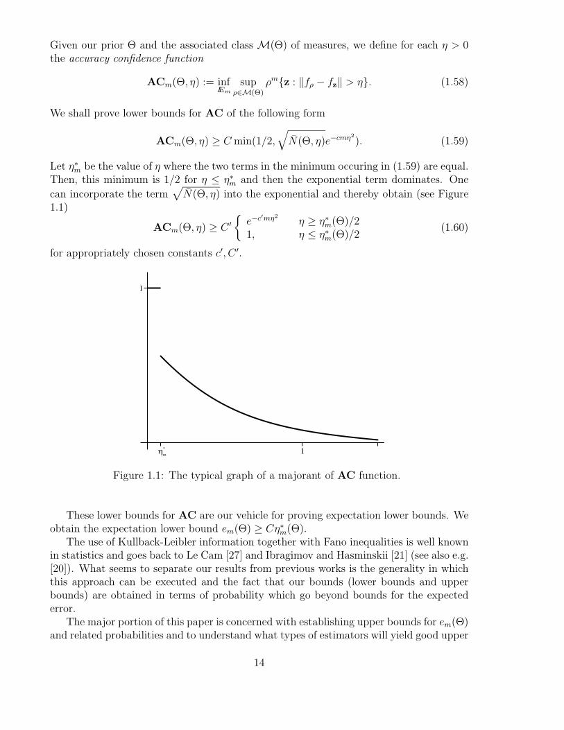
Given our prior # and the associated class M(#) of measures, we define for each # > 0the accuracy confidence function

ACm(#, #) := infIEm

sup!"M(!)

!m{z : 'f! $ fz' > #}. (1.58)

We shall prove lower bounds for AC of the following form

ACm(#, #) + C min(1/2,*

N(#, #)e#cm"2). (1.59)

Let #$m be the value of # where the two terms in the minimum occuring in (1.59) are equal.

Then, this minimum is 1/2 for # ( #$m and then the exponential term dominates. One

can incorporate the term+

N(#, #) into the exponential and thereby obtain (see Figure1.1)

ACm(#, #) + C %,

e#c"m"2# + #$

m(#)/21, # ( #$

m(#)/2(1.60)

for appropriately chosen constants c%, C %.

1

!*m 1

Figure 1.1: The typical graph of a majorant of AC function.

These lower bounds for AC are our vehicle for proving expectation lower bounds. Weobtain the expectation lower bound em(#) + C#$m(#).

The use of Kullback-Leibler information together with Fano inequalities is well knownin statistics and goes back to Le Cam [27] and Ibragimov and Hasminskii [21] (see also e.g.[20]). What seems to separate our results from previous works is the generality in whichthis approach can be executed and the fact that our bounds (lower bounds and upperbounds) are obtained in terms of probability which go beyond bounds for the expectederror.

The major portion of this paper is concerned with establishing upper bounds for em(#)and related probabilities and to understand what types of estimators will yield good upper

14

bounds. Typically we shall construct estimators that do not depend on # and show thatthey yield upper bounds for ACm(#, #) that have the same graphical behavior as inFigure 1.1:

ACm(#, #) (,

Ce#cm"2# + #m(#)

1, # ( #m(#).(1.61)

By integrating such probabilistic upper bounds we derive the upper bound em(#) (C#m(#). Notice that if #m(#) and #$

m(#) are comparable then we have a satisfactorydescription of ACm(#, #) save for the constants c, C.

It is possible to give estimators which provide upper bounds (both in terms of expecta-tion and probability) that match the lower bounds for all of the Sobolev and Besov classesthat are compactly embedded into C(X). The way to accomplish this is to use hypothesisclasses H with smaller entropy. For example, choosing for each class a proper "-net (de-pending on m) will do the job. This is shown in the follow up paper [25]. In particular,it implies the corresponding expectation estimates. Apparently, as was pointed out tous by Lucien Birge, similar expectation estimates can also be derived from the results in[4]. Also, we should mention that for the Sobolev classes W k(L!(X)) and expectationestimates, this was also proved by Stone (see again [19]).

The " net approach, while theoretically powerful, is not numerically implementable.We shall be interested in using other methods to construct estimators which may proveto be more numerically friendly. In particular, we want to see what we can expect fromestimators based on other methods of approximation including widths and nonlinear ap-proximation.

The estimation algorithms we construct in this paper will choose a hypothesis space H(which will generally depend on m) and take for fz the empirical least squares estimator(1.26) to the data z from H. There will be two types of choices for H:

Prior dependent estimators: These will start with a prior class # and constructan estimator using the knowledge of #. Such an estimator, tailored to # will typicallynot perform well on other prior classes.

Prior independent estimators: These estimators will be built independent of anyprior classes with the hope that they will perform well on a whole bunch of prior classes.

We shall say that an estimation algorithm (IEm) is universally convergent if fz con-verges in expectation to f! for each Borel measure ! on X. Such algorithms are sometimescalled consistent in statistics. We shall say that the algorithm is optimal in expectationfor the prior class # if

E!m('f! $ fz') ( C(#)em(#), m = 1, 2, . . . . (1.62)

We say that the algorithm is optimal in probability if

sup!"M(!)

!m{z : 'f! $ fz' > &} ( C1ACm(#, C2&), m = 1, 2, . . . , & > 0, (1.63)

with C1, C2 constants that may depend on #. We say that a learning algorithm is uni-versally optimal (in expectation or probability) for a class P of priors if it is optimalfor each # % P. We shall often construct estimators which are not optimal because ofthe appearance of an additional logarithmic term (log m)# for some ' > 0 in the case of

15

expectation estimates. We shall call such estimators semi-optimal. This is in particularthe case when we construct estimators that are e!ective for a wide class of priors (see e.g.§4.4): estimators that are e!ective for large classes of priors are called adaptive in thestatistics literature.

The simplest example of the type of upper bounds we establish is given in Theorem 4.1which uses Kolmogorov n-widths to build prior dependent estimators. If # is a compactset in C(X) whose Kolmogorov widths satisfy dn(#, C(X)) ( cn#r, then we choose H asLn * b(C(X)), where Ln is a near optimal n dimensional subspace for #. We show in §4.1

that when n := ( mln m)

12r+1 this will give an estimator fz = fz,H such that

E!m('f! $ fz') ( C(ln m

m)

r2r+1 , (1.64)

with C a constant depending only on r. That is, these estimators are semi-optimal in theirexpectation bounds. A corresponding inequality in probability is also established. Theestimate (1.64) applies to finite balls in Sobolev spaces, i.e. # = b(W s(Lp)) in which caser = s/d. It is shown that this again produces estimators which are semi-optimal provideds > d/2 and p + 2. The logarithm can be removed (for the above mentioned Sobolevspaces) by other methods (see [25] and in the case of expectation estimates Chapter 19of [19]).

One advantage of using Kolmogorov widths is that with them we can construct auniversal estimator. For example, we show in §4.4 that there is a single estimator thatgives the inequalities (1.64) provided a ( r < b with a > 0 an arbitrary but fixed constant.The constant b can be chosen arbitrarily in case of estimation in expectation but we onlyestablish this for r ( 1/2 for estimates in probability. It remains an open problem whetherthis restriction on r can be removed in the case of probability estimates.

Another method for constructing universal estimators based on adaptive partitioningis given in [5]. The estimator there is semi-optimal for a range of Besov spaces withsmoothness less than one (a restriction which comes about because the method usespiecewise constants for the construction of fz).

In §4.2, we show how to use nonlinear methods to construct estimators. These esti-mators can be considered as generalizations of thresholding operators based on waveletdecompositions. Recall that thresholding has proven to be very e!ective in a variety ofsettings in statistical estimation [17, 18]. For a range of Besov spaces, these esimators areproven to be semi-optimal.

In summary, as pertains to upper bounds, this paper puts forward a variety of tech-niques to obtain upper bounds and discusses their advantages and disadvantages. Insome cases these estimators provide semi-optimal upper bounds. In some cases they canbe modified (as reported on in subsequent papers) to obtain optimal upper bounds. Wealso highlight partial results on obtaining universally optimal estimators which we feel isan important open problem.

In (§5) we consider a variant of the learning problem in which we approximate a variantfµ of f!. Namely, we assume that d!X = µ dx is absolutely continuous and approximatethe function fµ := µf! from the given data z. We motivate our interest in this functionfµ with the above banking problem. One advantage gained in estimating fµ is that wecan provide estimates in Lp without having to go through L!.

16

We consider the results of this paper to be theoretical but some of the methods putforward could potentially be turned into numerical methods. At this point, we do notaddress the numerical feasibility of our algorithms. Our main interest is to understandwhat is the best performance we can expect (in terms of accuracy-confidence or expectederror decay with m) for the regression problem with various linear and nonlinear methods.

The use of entropy has a long history in statistical estimation. The use of entropyas proposed by Cucker and Smale [10] and also used here is similar in both flavor andexecution to other uses in statistics (see for example the articles [4], the book of Sara vande Geer [38] or the book of Gyorfi, Kohler, Krzyzak, and Walk [19]). We have tried toexplain the use of these concepts in a fairly accessible way, especially for researchers fromthe variious communities that relate to learning (statistics, functional analysis, probabilityand approximation) and moreover to show how other concepts of approximation such asKolmogorov widths or nonlinear widths can be employed in learning. They have someadvantages and disadvantages that we shall point out.

2 Priors described by smoothness or approximationproperties

The purpose of this section is to introduce the types of prior sets # that we shall employ.Since we are interested in priors for which em(#) tends to zero as m tends to infinity, wemust necessarily have # compact in L2(X, !X) for each ! % M(#). It is well known thatcompact subsets in Lp spaces (or C(X)) have a uniform smoothness when measured inthat space. Therefore, they are typically described by smoothness conditions. Anotherway to describe compact sets is through some type of uniform approximability of theelements of #. We shall use both of these approaches to describe prior sets. These twoways of describing priors are closely connected. Indeed, a main chapter in approximationtheory is to characterize classes A of functions which have a prescribed approximationrate by showing that A is a certain smoothness space. Space will not allow us to describethis setting completely - in fact it is a subject of several books. However, we wish topresent enough discussion for the reader to understand our viewpoint and to be able tounderstand the results we put forward in this paper. The reader may wish to skim overthis section and return to it only as necessary to understand our results on learning theory.

2.1 Smoothness spaces

We begin by discussing smoothness spaces in C(X) or in Lp(X) equipped with Lebesguemeasure. This is a classical subject in mathematical analysis. The simplest and bestknown smoothness spaces are the Sobolev spaces W k(Lp(X)), 1 ( p ( ), k = 1, 2, . . ..The space W k(Lp(X)) is defined as the set of all functions g % Lp(X) whose distributionalderivatives D#g, |'| = k, are also in Lp. The semi-norm on this space is

|g|W k(Lp(X)) :=)

|#|=k

'D#g'Lp(X). (2.1)

17

We obtain the norm 'g'W k(Lp(X)) for this space (and all other smoothness spaces in Lp(X))by adding 'g'Lp(X) to the semi-norm.

The family of Sobolev spaces is insu"cient for most problems in analysis because oftwo reasons. The first is that we would like to measure smoothness of order s when s > 0is not an integer. The second is that in some cases, we want to measure smoothness inLp(X) with p < 1. There are several ways to define a wider family of spaces. We shalluse the Besov spaces because they fit best with approximation and statistical estimation.

A Besov space Bsq(Lp(X)) has three parameters. The parameter 0 < p ( ) plays the

same role as in Sobolev spaces. It is the Lp(X) space in which we measure smoothness.The parameter s > 0 gives the smoothness order and is the analogue of k for Sobolevspaces. The parameter 0 < q ( ) makes subtle distinctions in these spaces.

The usual definition of Besov spaces is made by either using moduli of smoothness orby using Fourier transforms and can be found in many texts (we also refer to the paper[15]). For example, for 0 < s < 1, and p = ), the Besov space Bs

!(L!(X)) is the sameas the Lipschitz space Lip s whose semi-norm is defined by

|f |Lip s := supx1,x2"X

|f(x1) $ f(x2)||x1 $ x2|s

. (2.2)

We shall not give the general definition of Besov spaces in terms of moduli of smooth-ness or Fourier transforms but rather give, later in this section, an equivalent definitionin terms of wavelet decompositions (see §2.2) since this latter description is useful for un-derstanding some of our estimation theorems using wavelet decompositions.

It is well known when a finite radius ball b(W ) of a Sobolev or Besov spaces W iscompactly embedded in Lp(X). This is connected to what are called Sobolev embeddingtheorems. To describe these results, it will be convenient to have a pictorial descriptionof smoothness spaces. We shall use this pictorial description often in describing ourresults. We shall identify smoothness spaces with points in the upper right quadrant ofIR2. We write each such point as (1/p, s) and identify this point with a smoothness spaceof smoothness order s in Lp; this space may be the Sobolev space W k(Lp(X)) in the cases = k is an integer or the Besov space Bs

q(Lp(X)) in the general case s + 0. The points(1/p, 0) correspond to Lp(X) when p < ) and to C(X) when p = ). The compactsubsets of Lp(X) are easy to describe using this picture. We fix the value of p and weconsider the line segment whose coordinates (1/µ, s) satisfy 1/µ = s

d + 1p . This is the

so-called Sobolev embedding line for Lp(X). For any point (1/(, s) to the left of this line,any finite ball in the corresponding smoothness space is compactly embedded in Lp(X).Figure 2.1 depicts the situation for p = ), i.e. the spaces compactly embedded in C(X).

18

1/p

s

Sobolevembedding line

C(X)

Figure 2.2: The shaded region depicts the smoothness spaces embedded in C(X) whend = 2. The Sobolev embedding line has equation s = 2/p in this case.

Thus far, we have only described isotropic smoothness spaces, i.e. the smoothnessis the same in each coordinate. There are also important anistropic spaces which mea-sure smoothness di!erently in the coordinate directions. We describe one such family ofsmoothness spaces known as the Holder-Nikol’skii classes NHs

p , defined for s = (s1, . . . , sd)and 1 ( p ( ). This class is the set of all functions f % Lp(X) such that for eachlj = [sj] + 1, j = 1, . . . , d, we have

'f'p ( 1, '%lj ,jt f'Lp(X) ( |t|sj , j = 1, . . . , d, (2.3)

where %l,jt is the l-th di!erence with step size t in the variable xj. In the case d = 1,

NHsp coincides with the standard Lipschitz (0 < s < 1) or Holder (s + 1) classes. If

s1 = . . . = sd = s these classes coincide with the Besov classes Bs!(Lp(X)) (see §2.2).

2.2 Wavelet decompositions

In this section, we shall introduce wavelets and wavelet decompositions. These will beimportant in the construction of estimators later in this paper. Also, we shall use themto define the Besov spaces. There are several books which discuss wavelet decompositionsand their characterization of Besov spaces (see e.g. Meyer [30] or the survey [16]). Wealso refer to the article of Daubechies [13] for the construction of wavelet bases of the typewe want to use.

19

Let ) be a univariate scaling function which generates a univariate wavelet * whichhas compact support . For specificity, we take ) and * to be one of the Daubechies’ pairs(see [13]) which generate orthogonal wavelets. We define *0 := ) and *1 := *. Let E %

be the set of vertices of the unit cube [0, 1]d and let E := E % \ {(0, . . . , 0)} be the set ofnonzero vertices. We also let D denote the set of dyadic cubes in IRd and Dj the set ofdyadic cubes of side length 2#j. Each I % Dj is of the form

I = 2#j[k1, k1 + 1] " · · · " 2#j[kd, kd + 1], k = (k1, . . . , kd) % ZZd. (2.4)

For each 0 < p ( ), the wavelet functions

*eI(x) := *e

I,p(x) := 2jd/p*e1(2jx1 $ k1) · · ·*ed(2jxd $ kd), I % D, e % E, (2.5)

(normalized in Lp(IRd)) form an orthogonal system. Each locally integrable function f

defined on IRd has a wavelet decomposition

f =)

I"D

)

e"E

f eI *

eI , f e

I := f eI,p := -f,*e

I,p"., 1/p + 1/p% = 1. (2.6)

Here f eI = f e

I,p depends on the p-normalization that has been chosen but f eI *

eI is the same

regardless of p. We shall usually be working with L2 normalized wavelets. If this is notthe case, we shall indicate the dependence on p. The series (2.6) converges absolutely tof in the Lp(IR

d) norm in the case f % Lp(IRd) and 1 < p < ) and conditionally in the

case p = ) with L!(IRd) replaced by C(IRd).For any cube J , we shall denote by +(J) the side length of J . The wavelet functions

*eI all have compact support. We take I as the smallest cube that contains the support

of this wavelet. Then,+(I) ( A0+(I), (2.7)

where A0 depends only on the initial choice of the wavelet *.In order to define Besov spaces in terms of wavelet coe"cients, we let k be a positive

integer such that the mother wavelet * is in Ck(IRd) and has k vanishing moments. If0 < p, q ( ) and 0 ( s < k, then, for the p normalized basis {*e

I},

|f |Bsq(Lp(IRd)) :=

"--#

--$

%(!j=#! 2jsq

.(I"Dj

(e"E |f e

I |p/q/p

'1/q

, 0 < q < ),

sup#!<j<! 2js.(

I"Dj(

e#E|f e

I |p/1/p

, q = ).

(2.8)

defines the (quasi-semi)-norm for the Besov space Bsq(Lp(IR

d)). These spaces and normsare equivalent for di!erent choices of k (provided s < k) and are equivalent to the classicaldefinitions using moduli of smoothness as long as 1 ( p < ) or 0 < p < 1 and s/d >1/p $ 1. The quasi-norm in Bs

q(Lp(IRd)) is defined by

'f'Bsq(Lp(IRd)) := 'f'Lp(IRd) + |f |Bs

q(Lp(IRd)). (2.9)

If s is not an integer, we define W s(Lp(X)) := Bsp(Lp(X)) which serves to extend the

scale of Sobolev spaces to all s.

20

The wavelet decomposition (2.6) runs over all dyadic levels. There is an analogousdecomposition that runs only over j + j0 where j0 is any fixed integer. Let D+ := /j&j0Dj.Each locally integrable function on IRd has the wavelet decomposition

f =)

j&j0

)

I"Dj

)

e"Ej

f eI *

eI , f e

I := -f,*eI,p".. (2.10)

where Ej0 := E %, and Ej := E, j > j0. Here, for the case j = j0, the wavelets *eI are

replaced by the corresponding scaling functions )eI .

We can also describe Besov norms using this decomposition:

'f'Bsq(Lp(IRd)) :=

"--#

--$

%(!j=j0

2jsq.(

I"Dj

(e"E |f e

I |p/q/p

'1/q

, 0 < q < ),

supj&j0 2js.(

I"Dj(

e#E|f e

I |p/1/p

, q = ).

(2.11)

There are also wavelet decompositions for domains & # IRd. For our purposes, it willbe su"cient to describe such a basis for & = [0, 1]d. We start with a usual wavelet basisfor IR and construct a basis for [0, 1]. The bases for [0, 1] will contain all of the usualIR wavelet basis functions when these basis functions have supports strictly contained in[0, 1]. The other wavelets in this basis are obtained by modifying the IR wavelets whosesupports overlap [0, 1] but are not contained completely in [0, 1]. Notice that on anydyadic level there are only a finite number of wavelets that need to be modified. Fordetails on this construction see [6]. To get the basis [0, 1]d we take the tensor product ofthe [0, 1] basis. For the [0, 1]d wavelet system one has the same characterization of Besovspaces as given above.

2.3 Approximation spaces

Another way to describe priors is by imposing decay conditions on rates of approximation.One situation that we have already encountered is to impose a condition on entropynumbers. For example, for r > 0, we can consider a class # such that

"n(#) ( Cn#r. (2.12)

Such conditions are closely related to smoothness.Let us first describe this for entropy conditions in C(X). For the Sobolev spaces

W k(Lp(X)) (with respect to Lebesgue measure), we have

"n(b(W k(Lp(X)))C(X) ( Cn#k/d, n = 1, 2, . . . , (2.13)

provided k > d/p. Equivalently, this can be stated as

N(&, b(W k(Lp(X)))C(X) ( Cec0$! d

k , & > 0. (2.14)

Similar results hold for any of the Lipschitz or Besov spaces which are compactly embeddedinto C(X). If s > 0 and Bs

q(L% (X)) is a Besov space corresponding to a point to the leftof the Sobolev embedding line for C(X) then

"n(b(Bsq(L% (X)))C(X) ( Cn#s/d, n = 1, 2, . . . , (2.15)

21

where the constant C depends on the distance of (1/(, s) to the embedding line. We shallalso use priors that utilize Kolmogorov widths in place of entropy numbers. These areformulated in §4.1.

2.4 Approximation using a family of linear spaces

We introduce in this subsection a typical way of describing compact sets using approxima-tion. Let B be a Banach space and let Ln, n = 1, 2, . . ., be a sequence of linear subspacesof B with Ln of dimension ( n. For simplicity we assume that Ln # Ln+1. Typicalchoices for B are the Lp(X) spaces with respect to Lebesgue measure. Possible choicesfor Ln are space of algebraic or trigonometric polynomials. Note, that to maintain thecondition on the dimension of Ln, we would need to repeat these spaces of polynomials.

In this setting, we define for f % B

En(f) := En(f)B := infg"Ln

'f $ g'B (2.16)

which is the error in approximating f in the norm of B when using the elements of Ln.For any r > 0, we define the approximation class Ar := Ar(B, (Ln)) to be the set of

all f % B such that|f |Ar := sup

nnrEn(f). (2.17)

The functions in Ar can be approximated to accuracy |f |Arn#r when using the elementsof Ln.

There are slightly more sophisticated approximation classes Arq which make subtle

distinctions in approximation order through the index q % (0, )]. The seminorms forthese classes are defined by

|f |Arq

:= '(nrEn(f))'&q$, (2.18)

where '(,n)'q&q$ :=

(!n=1 |,n|q 1

n when q < ) and is the usual +! norm when q = ).A typical prior on the functions f! is to assume that f! is in a finite ball in Ar

q(B, (Ln))for a specific family of approximation spaces. The advantage of such priors over priors onsmoothness spaces is they can be defined for B = L2(µ) for arbitrary µ.

A large and important chapter of approximation theory characterizes approximationspaces as smoothness spaces in the case approximation takes place in Lp(X) with re-spect to Lebesgue measure. For example, consider the case of approximating 2--periodicfunctions on IT d by trigonometric polynomials of degree ( n which is a linear space ofdimension (2n + 1)d. Then, for any 1 ( p ( ) (with the case p = ) corresponding toC), we have

Arq((Ln), Lp(X))) = 0Brd

q (Lp), r > 0, 0 < q ( ), (2.19)

where the 0B indicates we are dealing with periodic functions. A similar result holds if wereplace trigonometric polynomials by spline functions of degree k on dyadic partitions withk + s $ 1. The corresponding results for wavelet approximation will be discussed in thefollowing subsection. The characterizations (2.19) provide a useful way of characterizingBesov spaces. It also shows that for many approximation methods the approximationclasses are identical.

22

2.5 Approximation using orthogonal systems

We discuss in this subsection the important case where approximation comes from anorthonormal system (we could equally well consider Riesz bases). Let us suppose that' :={*j}!j=1is a complete orthonormal system for L2(X) with respect to Lebesgue measure.The classical settings here are the Fourier and orthonormal wavelet bases. There are twotypes of approximation that we want to single out corresponding to linear and nonlinearmethods.

Any integrable function g has an expansion

g =!)

j=1

cj(g)*j; cj(g) :=

!

X

g*jdx. (2.20)

For a function g, we define

Sn(g) :=n)

j=1

cj(g)*j. (2.21)

This is the orthogonal projection of g onto the first n terms of the orthogonal basis '. Itis a linear method of approximation in that, for each n, we approximate from the linearspace Ln := span{*1, . . . ,*n} The error we incur in such an approximation is

En(g)p := 'g $ Sn(g)'Lp(X). (2.22)

As we have already noted in the previous section for the Fourier or wavelet bases, theapproximation classes Ar

q(Lp) are identical to the Besov spaces Bsq(Lp(X)), s = r/d (see

§2). In the case of the Fourier basis under lexicographic ordering, it is known that theprojector Sn is bounded on Lp(X), 1 < p < ). Therefore, for r > 0 and 1 < p < ),

g % Br!(Lp(X)) i! 'g $ Sn(g)'Lp(X) ( Cn#r/d, n = 1, 2 . . . , (2.23)

and the constant C is comparable with the norm of g in Br!(Lp(X)).

In the case of a wavelet orthonormal system (with their natural ordering from coarse tofine and lexicographic at a given dyadic scale), we have the same result as in (2.23) exceptthat the functions are no longer required to be periodic and the range of r is restrictedto r ( r0 where r0 depends on the smoothness and number of vanishing moments of themother wavelet.

There is a second way that we can approximate g from the orthogonal system {*j}which corresponds to nonlinear approximation. We define (n to be the set of all functionsS which can be written as a linear combination of at most n of the *j:

S =)

j""

cj*j, #($) ( n. (2.24)

In numerical considerations, we want to restrict the indices in (n in order to make thesearch for good approximations reasonable. We define (n,a as the set of S in (2.24) withthe added restriction $ # {1, . . . , na}. For 0 < p ( ),we define the error

%n.a(f)p := infS"#n,a

'f $ S'Lp(X). (2.25)

23

Now, let us consider the special case of approximation in L2(X). A best approximationfrom (n,a to a given g is simply given by

Gn,a(g) :=)

j"$n,a

cj(g)*j, (2.26)

where )n,a is the set of indices corresponding to the n largest (in absolute value) coe"cients|cj(g)| with j ( na Here we do not have uniqueness because of possible ties in the size ofthe coe"cients; these ties can be treated in any way to construct a )n,a. Thus,

%n,a(g)22 =

)

j /"$n,a

|cj(g)|2. (2.27)

Another way to describe the process of creating best approximations from (n,a is bythresholding. If . > 0, we denote by )(g,., a) the set of those indices j ( na such that|cj(g)| + .. Then,

T',a(g) :=)

j"$(',a,g)

cj(g)*j (2.28)

is a best approximation from (n,a to g in L2(X) where n := #()(., a, g)).It is also very simple, in the L2(X) approximation case, to describe the approximation

classes. For example, a function g % Ar!(L2(X)), i.e. %n,a(g)2 ( C0n#r, n = 1, 2, . . ., if

and only if the following hold:

#()(., a, g)) ( C1.#% , . > 0,

1

(= r +

1

2(2.29)

andEna(g)2 ( C1n

#r, n = 1, 2, . . . (2.30)

and the constants C1 and C0 are comparable.A case of special interest to us will be when ' is a wavelet basis (see §2). In this case,

the characterizations (2.29), (2.30) are related to Besov spaces. For example, wheneverg % Brd

% (L% (X)), the condition (2.29) is satisfied. As we have already noted, the condition

(2.30) is characterized by g % Brd/a! (L2(X)). Because of the Sobolev embedding theorem,

both conditions will be satisfied if g % Brdµ (Lµ(X)) provided

r +1

2$ 1

µ+ r

a. (2.31)

In other words, if the mother wavelet for ' is in Ck and has k vanishing moments, thenwe have

Remark 2.1 If a > 0, then conditions (2.29) and (2.30) are satisfied for all f % Brdµ (Lµ(X))

provided rd < k and (2.31) holds.

24

2.6 Universal methods of approximation

In evaluating a particular approximation process, one can look at the classes of functionsfor which the approximation process gives optimal or near optimal performance. Forexample, if we use a sequence (Ln) of linear spaces of dimension n, we say this sequenceis near optimal for approximating the elements of the compact set K in the norm of theBanach space B if

dist(K,Ln)B ( Cdn(K,B) (2.32)

where dn is the Kolmogorov width of K. The same notion can be given for nonlinearmethods of approximation except now we would compare performance against nonlinearwidths.

Some approximation systems are near optimal for a large collection of compact sets K.We say that a sequence (Ln) of linear spaces of dimension n are universally near optimal forthe collection K of compact sets K if (2.32) holds for each K % K with a universal constantC > 0. That is, the one sequence of linear space (Ln) is simultaneously near optimal forall these compact sets. There is the analogous concept of universally near optimal withrespect to nonlinear methods. In this case, one replaces in (2.32) the linear space Ln

by nonlinear spaces depending on n parameters and replaces the Kolmogorov width bythe corresponding nonlinear width. In the learning problem we shall introduce a similaruniversal concept for learning algorithms. Therefore we want to briefly describe what isknown about universality in the approximation setting for the purposes of comparisonwith our later results.

Let us begin the discussion by considering a wavelet system of compactly supportedwavelets from Ck(X) which have vanishing moments up to k. The Besov space Bs

q(L% )is compactly embedded in Lp if and only if s > (d/( $ d/p)+. For any fixed & > 0, let Kbe the set consisting of all unit balls u(Bs

q(Lp)) with s $ d/( + d/p + & and 0 < s < k.Then, nonlinear wavelet approximation based on thresholding is near optimal for Lp(X)approximation (Lebesgue measure) for all of the sets K % K.

The standard wavelet system is suitable only to approximate isotropic classes. It is amore subtle problem to find systems that are universal for both isotropic and anisotropicclasses. We shall discuss this topic in the case of multivariate periodic functions.

We have introduced earlier in §2.1 the collection of anisotropic Holder-Nikol’skii classesNHs

q . It is known (see for instance [36]) that the Kolmogorov n-widths of these classesbehave asymptotically as follows:

dn(NHsq , Lq) 1 n#g(s), 1 ( q ( ), (2.33)

where

g(s) := (d)

j=1

s#1j )#1.

In the case of periodic functions, we can find for each s a near optimal subspace Ln ofdimension n for NHs

q in Lq, i.e. it satisfies (2.32). The space Ln can be taken for exampleas the set of all trigonometric polynomials with frequencies k satisfying the inequalities

|kj| ( 2g(s)l/sj , j = 1, . . . , d, (2.34)

25

where l is the largest integer such that the number of vectors k satisfying the aboveinequalities is ( n.

Notice that the subspaces Ln described by (2.34) are di!erent for di!erent s andtherefore do not satisfy our quest for a universally near optimal approximating method.For given a,b with 0 < aj < bj, j = 1, . . . , d, and a given p, we consider the class

Kq,p([a,b]) := {u(NHsq ) : aj ( sj ( bj, j = 1, 2, . . . , d, g(a) > (1/q $ 1/p)+}. (2.35)

Each of the sets in Kp,p is compact in Lp(X). It can be shown that there does not exista sequence (Ln) of linear space Ln of dimension n which is universally optimal for thiscollection of compact sets. In fact, it is proved in [36] that for a sequence of linear spaces(Ln) to satisfy (2.32) for Kp,p then one must necessarily have dim(Ln) + c(log n)d#1n.Moreover, this result is optimal in the sense that we can create a sequence of spaces withthis dimension that satisfy (2.32).

If we turn to nonlinear methods then we can achieve universality for the class (2.35).We describe one such result. We consider the library O consisting of all orthonormal basesO on X. For each n and O, we consider the error %n(f,O)p of n term approximation whenusing the orthogonal basis O (see the definition (2.25) with a = )). Given a set K, wedefine

%n(K,O)p := supf"K

%n(f,O)p. (2.36)

and%n(K,O)p := sup

f"KinfO"O

%n(f,O)p. (2.37)

We say that the basis O is near-optimal for the class K if

%n(K,O)p ( C%n(K,O)p, n = 1, 2, . . . . (2.38)

In analogy to the linear setting, we say that O is universally near-optimal for a collectionK of compact sets K if (2.38) holds for all K % K with an absolute constant. It is shownin [37] that there exists an orthogonal basis which is universally near-optimal for thecollection Kq,p defined in (2.35) for 1 < q < ), 2 ( p < ). Also, for each K = u(NHs

q ),%n(K,O)p 2 n#g(s), 1 < q < ), 2 ( p < ).

3 Lower bounds

In this section, we shall establish lower bounds for the accuracy that can be attained inestimating the regression function f! by any learning algorithm. We will establish ourlower bounds in the case X = [0, 1]d, Y = [$1, 1] and Z = X " Y . In going further inthis paper, these lower bounds will serve as a guide for us in terms of how we would likespecific algorithms to perform.

We let # be a given set of functions defined on X which corresponds to the prior weassume for f!. We define, as in the introduction, the class M(#) of all Borel measures !on Z for which f! % # and define em(#) by (1.56). We shall even be able to prove lowerbounds with weaker assumptions on the learning algorithms IEm. Namely, in addition

26

to allowing the learning algorithm to know #, we shall also allow the algorithm to knowthe marginal !X . To formulate this, we let µ be any Borel measure defined on X and letM(#, µ) denote the set of all ! % M(#) such that !X = µ and consider

em(#, µ) := infIEm

sup!"M(!,µ)

E!m('f! $ fz'L2(X,µ)). (3.1)

We shall give lower bounds for em and related probabilities. To prove these lower boundswe introduce a di!erent type of entropy.

3.1 Tight entropy

We shall establish lower bounds for em in terms of a certain variant of the Kolmogoroventropy of # which we shall call tight entropy. This type of entropy has been used toprove lower bounds in approximation theory. Also, a similar type of entropy was used byYang and Barron [41] in statistical estimation. The entropy measure that we shall use isin general di!erent from the Kolmogorov entropy, but, as we shall show later, for classicalsmoothness sets #, it is equivalent to the Kolmogorov entropy and therefore our lowerbounds will apply in these classical settings.

We assume that # # L2(X,µ). Let 0 < c0 ( c1 < ), be two fixed real numbers. Wedefine the tight packing numbers

N(#, &, c0, c1) := sup{N : 3 f0, f1, ..., fN % #, with c0& ( 'fi $fj'L2(X,µ) ( c1&, 4i ,= j}.(3.2)

We will use the abbreviated notation N(&) := N(#, &, c0, c1), when there is no ambiguityon the choice of the other parameters. Obviously, if # is a subset of a normed space, thenfor all R > 0, N(R#, &, c0, c1) = N(#, $

R , c0, c1).

3.2 The main result

Let us fix any set # and any Borel measure µ defined on X. We set M := M(#, µ) asdefined above. We also take c0 < c1 in an arbitrary way but then fix these constants. Forany fixed & > 0, we let {fi}N

i=0, with N := N(&), be a net of functions satisfying (3.2). Toeach fi, we shall associate the measure

d!i(x, y) := (ai(x)d&1(y) + bi(x)d&#1(y))dµ(x), (3.3)

where ai(x) := (1 + fi(x))/2, bi(x) := (1 $ fi(x))/2 and d&( denotes the Dirac delta withunit mass at $. Notice that (!i)X = µ and f!i = fi and hence each !i is in M(#, µ).

We have the following theorem.

Theorem 3.1 Let 0 < c0 < c1 be fixed constants. Suppose that # is a subset of L2(µ)with packing numbers N := N(&) := N(#, &, c0, c1). In addition suppose that for & > 0,the net of functions {fi}N

i=0 in (3.2) satisfies 'fi'C(X) ( 1/4, i = 0, 1, . . . , N . Then forany estimator fz we have for c2 := e#3/e and some i % {0, 1, . . . , N}

!mi {z : 'fz $ fi'L2(X,µ) + c0&/2} + min(1/2, c2

*N(&)e#2c21m$2

), 4& > 0, m = 1, 2, . . . ,

(3.4)

27

and for some ! % M(#, µ), we have

E!m('fz $ f!'L2(X,!X)) + c0&$/4, (3.5)

whenever ln N(&$) + 4c21m(&$)2.

The remainder of this subsection will be devoted to the proof of this theorem.The first thing we wish to observe is that the measures !i are close to one another. To

formulate this, we use the Kullback-Leibler information. Given two probability measuresdP and dQ defined on the same measure space and such that dP is absolutely continuouswith respect to dQ, we write dP = gdQ and define

K(P,Q) :=

!ln gdP =

!g ln gdQ. (3.6)

If dP is not absolutely continuous with respect to dQ then K(P,Q) := ).It is obvious that

K(Pm, Qm) = mK(P,Q). (3.7)

Lemma 3.2 For any Borel measure µ and the measures !i defined by (3.3), we have

K(!i, !j) ( 16

15'fi $ fj'2

L2(X,µ), i, j = 0, . . . , N . (3.8)

Proof: We fix i and j. We have d!i(x, y) = g(x, y)d!j(x, y), where

g(x, y) =1 + (sign y)fi(x)

1 + (sign y)fj(x)= 1 +

(sign y)(fi(x) $ fj(x))

1 + (sign y)fj(x). (3.9)

Thus,

2K(!i, !j) =

!

X

Fi,j(x)dµ(x) (3.10)

where

Fi,j(x) := (1 + fi(x)) ln(1 +fi(x) $ fj(x)

1 + fj(x)) + (1 $ fi(x)) ln(1 $ fi(x) $ fj(x)

1 $ fj(x)). (3.11)

Using the inequality ln(1 + u) ( u, we obtain

Fi,j(x) ( (fi(x) $ fj(x))

,1 + fi(x)

1 + fj(x)$ 1 $ fi(x)

1 $ fj(x)

0

=2|fi(x) $ fj(x)|2

1 $ fj(x)2( (32/15)|fi(x) $ fj(x)|2.

Putting this in (3.10), we deduce (3.8). !To prove the lower bound stated in Theorem 3.1, we shall use the following version of

Fano inequalities which is a slight modification of that given by Birge [41].

28

Lemma 3.3 Let A be a sigma algebra on the space &. Let Ai % A, i % {0, 1, . . . , n}such that 4i ,= j, Ai * Aj = 5. Let Pi, i % {0, 1 . . . , n} be n + 1 probability measures on(&,A). If

p :=n

supi=0

Pi(& \ Ai),

then either p > nn+1 or

infj"{0,1,...,n}

1

n

)

i'=j

K(Pi, Pj) + 'n(p), (3.12)

where

'n(p) := (1 $ p) ln (1 $ p

p)(

n $ p

p) $ p ln (

n $ p

np) = ln n + (1 $ p) ln (

1 $ p

p) $ p ln (

n $ p

p).

(3.13)

Proof The proof of this lemma follows the same arguments as Birge and therefore weshall only sketch the main steps. We begin with the following duality statement whichholds for probability measures P and Q:

K(P,Q) = sup{!

fdP,

!exp fdQ = 1}. (3.14)

This result goes back at least to the Sanov theorem (see a.e. Dembo-Zeitouni [12] ).Taking f = ./A in (3.14), we find that for all A % A and . % IR, we have

K(P,Q) + .P (A) $ log[(exp. $ 1)Q(A) + 1] = .P (A) $ 0Q(A)(.), (3.15)

where for 0 < q < 1, . % IR

0q(.) := log[(exp. $ 1)q + 1] = log[q exp. + 1 $ q]

Note that 0q(.) is convex in ., while it is concave and nondecreasing in q if . + 0.If we apply (3.15) to Pi and P0 for each i = 1, . . . , n and then sum we obtain

1

n

n)

i=1

K(Pi, P0) + .1

n

n)

i=1

Pi(Ai) $ 1

n

n)

i=1

0P0(Ai)(.). (3.16)

Obviously, if . + 0, then

.1

n

n)

i=1

Pi(Ai) + .n

infi=0

Pi(Ai) = .(1 $ p).

Using convexity and monotonicity, we have for . % IR

$ 1

n

n)

i=1

0P0(Ai)(.) + $0 1n

(ni=1 P0(Ai)(.) = $0 1

n P0((ni=1Ai)(.).

29

Using again the fact that q 6& 0q(.) is non decreasing, together with P0(/ni=1Ai) (

(1 $ P0(A0)) = P0(Ac0) ( p gives that for . + 0,

$0 1n P0((n

i=1Ai)(.) + $0 pn(.).

Therefore, 4. + 0,1

n

n)

i=1

K(Pi, P0) + .(1 $ p) $ 0 pn(.)

To complete the proof, we define

sup'&0

(.t $ 0q(.) =: 0$q(t).

One easily checks that

0$q(t) =

"#

$

0 if t < qt log( t

q ) + (1 $ t) log( 1#t1#q ) if q ( t ( 1

) if t > 1.

We now take q = p/n and t = 1 $ p and use the above in (3.16), we obtain

1

n

n)

i=1

K(Pi, P0) + 0$p/n(1 $ p). (3.17)

We can replace P0 by Pj for any j % {0, 1, . . . , n} in the above argument. Using this weeasily derive (3.13) which completes the proof of the lemma . !

Proof of Theorem 3.1 We define Ai := {z : 'fz $ fi'L2(µ) < c0&/2}, i = 0, . . . , N =N(#, &) with c0 the constant in (3.2). Then, the sets Ai are disjoint because of (3.2). Weapply Lemma 3.3 with our measures !m

i and find that either p + 1/2 or

2c21m&2 + 'N(p) + $ ln p+(1$p) ln N+(1$p) ln (1 $ p)+2p ln p + $ ln p+(1/2) ln N$3/e,

(3.18)where we have used that x ln x has the minimum value $1/e on [0, 1]. From (3.18), wederive (3.4). Now given &$ such that

+N(&$) + e2c1m($$)2 , we have from (3.4) that for

this &$ there is an i such that with ! = !i, we have

!m('fz $ f!'L2(!X) > c0&$/2) + 1/2. (3.19)

It follows that for any & ( &$, (3.19) also holds. Integrating with respect to & we obtain(3.5). This completes the proof of the theorem. !

3.2.1 Lower bounds for Besov classes

In this subsection, we shall show how to employ Theorem 3.1 to obtain lower bounds forthe learning problem with priors given as balls in Besov spaces (with these spaces defined

30

relative to Lebesgue measure). We first show how to obtain lower bounds for the prior# = b(Bs

q(L!(X)), s > 0, 0 < q ( ). We shall take X = [0, 1]d and dµ to be Lebesguemeasure. From this, one can deduce the same lower bounds for any minimally smoothdomains X with again dµ Lebesgue measure.

To construct an appropriate net for # we shall use tensor product B-splines on dyadicpartitions. We fix a & > 0 and choose j as the smallest integer such that 2#js ( &. Forany j = 1, 2, . . . and for k := 7s8, there are + 2jd tensor product B-splines of degree kat the dyadic level j. They each have support on a cube with side length 2#jk. We canchoose J + c2jd of these B-splines with disjoint supports. We label these as {0i}J

i=1 andnormalize them in L2(X). Then , '0i'L% ( c

9J .

We construct a net of functions fi which satisfy (3.2). As was shown in [23], we canchoose at least eJ/8 subsets $i # {1, . . . , J} such that for each i, j we have #(($i \ $j) /($j \ $i)) + J/4. For each such $i, we define

fi :=&9J

)

j""i

0j. (3.20)

This net {fi} of functions satisfy

&/2 ( 'fi $ fj'L2(µ) ( &. (3.21)

Also,'fi'C(X) ( c& (3.22)

where we used our remark on the supports of the 0i. The inequality (3.22)means that ourcondition 'fi'L%(X) of Theorem 3.1 will be satisfied provided & < &0 for a fixed &0 > 0.

We next want to show that each of the functions fi is in # provided we take theradius of this ball su"ciently large (depending only on d). For this, we consider theapproximation of a given function f % C(X) by linear combinations of all tensor productB-splines from dyadic level n. If we denote by E %

n(f) the error of approximation in C(X)to f by this space of splines , then we have

E %n(fi) ( c

,&, n ( j0, n > j.

(3.23)

This means that!)

n=1

[2nsE %n(fi)]

q ( &qj)

n=1

2nsq ( Cq&q2jsq ( Cq, (3.24)

where C depends only on q and d. The convergence of the sum in (3.24) is a characteri-zation of the Besov space Bs

q(L!(X)) by linear approximation as noted in §2.3.We have just proven that N(&, Bs

q(L!)) + eJ/8 provided & ( J#s/d. Equivalently, we

have proved that N(&,#) + c3e$!ds for each 0 < & < &0. Let us now apply Theorem 3.1.

Estimate (3.5) gives thatem(#) + em(#, dµ) + c0&

$/4 (3.25)

31

for any &$ which satisfies ln N(&$) + 4c1m(&$)2 + 1, i.e. provided (&$)#d/s + cm(&$)2.From this, we obtain

em(#) + em(#, dµ) + cm# s2s+d , m = 1, 2, . . . . (3.26)

A similar analysis shows that (3.4) gives that for any estimator fz,

sup!"M(!)

!m{z : 'fz $ f!'L2(X,!X) + c&} +,

1/2, & ( 2&$,Ce#c$2m, & > 2&$,

(3.27)

where &$ = cm# s2s+d is the turning value as described above. These are the lower bounds

we want for the Besov space Bsq(L!(X)). Because each Besov space Bs

q(Lp(X)) containsthe corresponding Bs

q(L!(X)), we obtain the same lower bounds for these spaces.

4 Estimates for f!

In this section, we shall introduce several methods for constructing estimators fz. Typi-cally, we assume that f! % # where # = b(W ) is a ball in a space W which is assumedto have a certain approximation property. We then use this approximation property tochoose a set H and define the estimator fz % H as the least squares fit to the data zfrom H. We then prove an estimate for the rate that fz approximates f! (in L2(X, !X)).These estimates will typically give (save for a possible logarithmic term) the optimal ratefor this class.

4.1 Estimates for classes based on Kolmogorov widths.

In this subsection, we shall assume that # # bR0(C(X)) for some R0 and that its Kol-mogorov widths (1.14) satisfy 6

dn(#, C(X)) ( Cn#r, n = 1, 2, . . . . (4.1)

This means that for each n, there is a linear subspace Ln of C(X) of dimension n suchthat

dist(#,Ln)C(X) ( C1n#r, n = 1, 2 . . . . (4.2)

There is an inequality of Carl [7] that compares entropy to widths. It says that whenever(4.1) holds then

"n(#, C(X)) ( C2n#r n = 1, 2, . . . . (4.3)

Therefore, the prior f! % # is typically stronger than the corresponding assumption (1.46).The following theorem shows that under the assumption (4.1), we can derive a better

estimate than that given in Corollary 1.1

6We shall use the following convention about constants. Those constants whose value may be impor-tant later will be denoted with subscripts. Constants with no subscript such as c, C can vary with eachoccurrence even in the same line.

32

Theorem 4.1 Let f! % # where # # bR0(C(X)) and # satisfies (4.2). Given m + 2, we

take n := ( mln m)

12r+1 and define H := Hm := bR(C(X)) * Ln where R := M + C1. Then,

the least squares estimator fz for this choice of H satisfies

!m{z : 'f! $ fz' + #} ( C

,e#cm"2

# + #m

1, # ( #m,(4.4)

where #m := C(ln m/m)r

1+2r and the constants c, C depend only on C1 and M . In partic-ular,

E!m('f! $ fz') ( C(ln m

m)

r2r+1 (4.5)

where C is also an absolute constant.

Proof: By our assumption, there is a 0n % Ln such that 'f! $ 0n'L%(X) ( C1n#r.Since 'f!'L%(X) ( M , we have '0n'L%(X) ( M + C1n#r. This gives that 0n % H for ourchoice of R = C1 + M . Therefore, with this choice of R, and H := bR(C(X)) * Ln, wehave the estimate

dist(f!,H)C(X) ( C1n#r. (4.6)

It follows thatdist(f!,H)L2(X,!X) ( C1n

#r. (4.7)

For any # > 0, we have that the covering numbers of H satisfy (see p. 487 of [29])

N(H, #) ( (C/#)n. (4.8)

Combining this with (4.6), we obtain from (1.44)

'f! $ fz' ( C1n#r + #, z % $m(#), (4.9)

where!m{z /% $m(#)} ( 2(C3/#

2)ne#c2m"2. (4.10)

The critical turning value in (4.10) occurs when n[ln C3 + 2| ln #|] = c2m#2. This gives

!m{z /% $m(#)} (,

Ce#cm"2# + #m

1, # ( #m,(4.11)

where #m as defined in the theorem. This proves (4.4). The estimate (4.5) follows byintegrating (4.4) (see (1.19)). !

Let us mention some spaces W which satisfy the property (4.1). If s > d/2 and p + 2,then a theorem of Kashin can be used to deduce (4.1) for W = W s(Lp(X)) where theseSobolev spaces are defined with respect to Lebesgue measure. Note that the assumptions > d/2 + d/p guarantees that any ball b(W s(Lp(X)) is compact in C(X). We thereforehave the following corollary

Corollary 4.2 If W = W s(Lp(X)) with s > d/2 and p + 2, then the assumptions andconclusions of Theorem 4.1 hold for any ball b(W ).

33

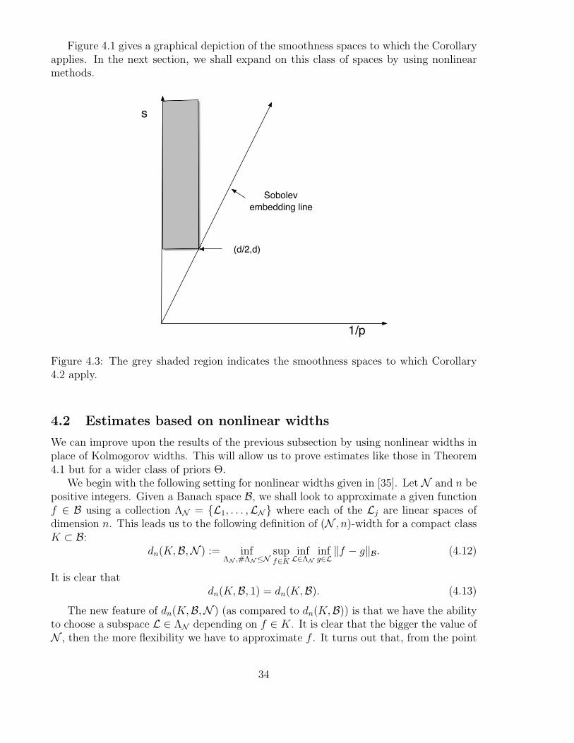
Figure 4.1 gives a graphical depiction of the smoothness spaces to which the Corollaryapplies. In the next section, we shall expand on this class of spaces by using nonlinearmethods.

1/p

s

Sobolevembedding line

(d/2,d)

Figure 4.3: The grey shaded region indicates the smoothness spaces to which Corollary4.2 apply.

4.2 Estimates based on nonlinear widths

We can improve upon the results of the previous subsection by using nonlinear widths inplace of Kolmogorov widths. This will allow us to prove estimates like those in Theorem4.1 but for a wider class of priors #.

We begin with the following setting for nonlinear widths given in [35]. Let N and n bepositive integers. Given a Banach space B, we shall look to approximate a given functionf % B using a collection $N = {L1, . . . ,LN} where each of the Lj are linear spaces ofdimension n. This leads us to the following definition of (N , n)-width for a compact classK # B:

dn(K,B,N ) := inf"N ,#"N)N

supf"K

infL""N

infg"L

'f $ g'B. (4.12)

It is clear thatdn(K,B, 1) = dn(K,B). (4.13)

The new feature of dn(K,B,N ) (as compared to dn(K,B)) is that we have the abilityto choose a subspace L % $N depending on f % K. It is clear that the bigger the value ofN , then the more flexibility we have to approximate f . It turns out that, from the point

34

of view of our applications, the following case

N 1 nan,

where a > 0 is a fixed number, plays an important role.Let us assume that # is a compact subset of C(X) which satisfies # # bR0(C(X)),

for some R0 > 0 and also satisfies the following estimates for the nonlinear Kolmogorovwidths

dn(#, C(X), nan) ( C1n#r, n = 1, 2, . . . . (4.14)

Then by [35]"n(#, C(X)) ( C2(ln n/n)r, n = 2, 3, . . . . (4.15)

In the theorem that follows, we shall not be able to use Theorem C* directly sincethe set H we shall choose for the empirical least squares minimization will not be convex.Therefore, we first prove an extension of Theorem C* which deals with the nonconvexsetting.

Theorem 4.3 Let H be a compact subset of C(X). Assume that for all f % H, f : X & Yis such that |f(x) $ y| ( M a.e. Then, for all # > 0

!m{z : 'fz,H $ fH'2 + #} ( N(H, #/(24M))2e#m!

C(M,K) (4.16)

provided 'f! $ fH'2 ( K#.

Proof The proof is similar to the proof of Theorem C* from [CS]. In the proof of TheoremC*, one uses the estimate (1.31) which we recall follows from the convexity assumption.In its place we shall use the estimate

'f $ fH'2 ( 2(E(f) $ E(fH) + 2K#), f % H. (4.17)

To prove this we note that

'f $ fH'2 ( 2{'f $ f!'2 + 'fH $ f!'2} = 2{E(f) $ E(fH) (4.18)

+ E(fH) $ E(f!) + 'fH $ f!'2} = 2{E(f) $ E(fH) + 2'fH $ f!'2}.

Thus, (4.17) follows by placing our assumption 'f! $ fH'2 ( K# into (4.18). The proofof Theorem 4.3 can now be completed in the same way as the proof of Theorem C*.

Theorem 4.4 Let # satisfy (4.14). If f! % # and m % {1, 2, . . .}, then there exists anestimator fz such that

!m{z : 'f! $ fz' + #} ( C

,e#cm"2

# + #m

1, # ( #m,(4.19)

where #m := C2(ln m/m)r

1+2r . In particular,

E!m('f! $ fz') ( C(ln m

m)

r2r+1 (4.20)

where C is also an absolute constant.

35

Proof: The proof is very similar to that of Theorem 4.1. Given m, we shall choosen := ( m

ln m)1

2r+1 . For this value of n let N := nan with a > 0 given in (4.14). For this N andn there is a collection $N of n-dimensional subspaces which realizes the approximationorder (4.14). Here #($N ) = N . Thus for any f % b(W ) there is an L % $N and a 0n % Lsuch that 'f $ 0n'C(X) ( C1n#r. It follows that '0n'C(X) ( R0 + C1 =: R. We nowconsider the following set

H := /L""NL * bR(C(X)). (4.21)

Then, it is clear that the entropy numbers for H satisfy

N(H, #) ( N (C/")n. (4.22)

We define our estimator for z % Zm by

fz := arg minf"H

Ez(f).

Using (4.22) with (4.14), we obtain from (4.16)

'f! $ fz' ( C1n#r + #, z % $m(#), (4.23)

where!m{z /% $m(#)} ( 2N (C3/#

2)ne#c2m"2(4.24)

The critical turning value in (4.24) occurs when an ln n+n[ln C3 +2| ln #|] = c2m#2. Thisgives

!m{z /% $m(#)} (,

Ce#cm"2# + #m,n

1, # ( #m,(4.25)

with #m,n := C2

*n ln m

m provided we choose C2 large enough. This proves (4.19) and (4.20)

follows by integrating (4.19). !We give next an illustrative setting in which Theorem 4.4 can be applied. Let ' :=

{*j}!j=1 be a Schauder basis for C(X). We fix an arbitrary a > 0 and consider for eachpositive integer n, the space (n,na of all functions

)

j"$

cj*j, ) # {1, . . . , na}, #()) ( n. (4.26)

Thus we are in the same situation as in §2.5 except that we do not necessarily use anorthogonal system. As in §2.5, given any f % C(X), we define

%n,na(f)! := infg"#n,na

'f $ g'C(X). (4.27)

This is the error of n-term approximation using ' except that we have imposed the extracondition on the indices.

We can realize this form of approximation as a special case of the approximation usedin the definition of (N , n) widths with N := nan. Namely we consider the set of all ndimensional subspaces spanned by n elements of ' with the restriction that the indicesof these elements come from {1, . . . , na}. There are ( N of these subspaces.

36

To carry this example further, we suppose that X = IRd and ' := {*'} is a waveletbasis for IRd as described in §2.6. Approximation from (n,na is then n-term waveletapproximation but with the restriction on the indices of basis functions. This form ofapproximation is used in encoding images and its approximation properties are well un-derstood (see [9]).

Corollary 4.5 Suppose that f! % b(W ) with W = W s(Lp(X))) with s > d/p or thatW = Bs

q(Lp(X) with s > d/p and 0 < q ( ). Let H = Hm := (n,na * bR(C(X)) be

defined as above using the wavelet basis with n := ( mln m)

d2s+d and a > s $ d/p . Then, the

least squares estimator fz for this choice of H satisfies

!m{z : 'f! $ fz' + #} ( C

,e#cm"2

# + #m

1, # ( #m,(4.28)

where #m := C2(ln m/m)s

2s+d . In particular,

E!m('f! $ fz') ( C(ln m

m)

s2s+d (4.29)

where C is also an absolute constant.

Proof: It was shown in [9] that for this choice of a, the above form of restricted approx-imation satisfies

dist(f,H)C(X) ( C1n# s

d . (4.30)

Therefore, we can apply Theorem 4.4 and derive the Corollary. !Notice that the Corollary applies to each smoothness space that is compactly em-

bedded in C(X), i.e. to each smoothness space depicted in the shaded region of Figure2.1.

4.3 Estimates for f! using interpolation

We want to show in this section how techniques from the theory of interpolation of linearoperators can be used to derive estimators fz to f!. The idea of using interpolation ofoperators was suggested in the paper of Smale and Zhou [32] in the setting of Hilbertspaces but they do not culminate this approach with concrete estimates since in theHilbert space setting we do not have the analog of Theorem C*. We shall see that thisapproach falls a little short of giving the optimal decay (O(m# s

2s+d )) for Sobolev or Besovspaces of smoothness s.

We shall use interpolation with C(X) (equivalently L!(X)) as one of the end pointspaces. For the other end point space we can take W0 = W0(X) where W0 # C(X) isa smoothness space embedded in C(X). A space V is called an interpolation space forthis pair (C(X),W0) if each linear operator T which is bounded on both C(X) and W0 isautomatically bounded on V . The real method of interpolation gives one way to generateinterpolation spaces by using what is called the K-functional:

K(f, t; C(X),W0) := infg"W0

'f $ g'C(X) + t|g|W0 . (4.31)

37

We mention only one setting for this which will su"ce for our analysis. Given 0 < 1 < 1,we define V) := (C(X),W0)),! to be the set of all f % C(X) such that

|f |V#:= sup

t>0t#)K(f, t : C(X),W0) (4.32)

is finite. So, membership in V) means that f can be approximated by a g % W0 toaccuracy Ct) while the norm of g in W0 is ( Ct)#1:

'f $ g'C(X) + t|g|W0 ( |f |V#t). (4.33)

We shall take for W0 any Besov space W0 = Bsp(Lp(X)) which is compactly embedded

in C(X). As mentioned earlier, we get a compact embedding if and only if s > d/p. It isknown that the covering numbers for the unit ball u(W0) satisfy

N(#, u(W0)) ( C0ec0"!d/s

, # > 0, (4.34)

with the constants depending only on W0.Our main result of this section is the following.

Theorem 4.6 Let W0 be a Besov space Bsp(Lp(X)) such that u(W0) is compactly em-

bedded in C(X). If f! % u(V)) where V) = (C(X),W0)),! and 1 := r/s, then we take

H := bR(W0) with R := ms!r

2r+d+rd/s . The least squares minimizer fz for this choice of Hsatisfies

!m{z : 'f! $ fz' + #} ( C

,e#cm"2

# + #m

1, # ( #m,(4.35)

where #m := C2m# r

2r+d+rd/s . In particular,

E('f! $ fz') ( Cm# r2r+d+rd/s (4.36)

where C is a constant depending only on s and W0.

Remark 4.7 By rescaling, we can also treat the prior f! % bR0(V)) for any R0 > 0.

Proof: As usual, we only need to prove (4.35). We shall use the K-functional (4.31)but leave the choice of t open at the beginning. From the definition of V) we know thatthere is a function g % W0 such that

'f! $ g'C(X) + t|g|W0 ( t)|f!|V#( t). (4.37)

Since fH is a best approximation to f! from H in the norm ' ·' , it follows that the biasterm satisfies

'f! $ fH' ( 'f! $ g' ( 'f! $ g'C(X) ( t). (4.38)

The function g is in bR1(W0) where R1 = t)#1. Since N(#, bR1(W0)) = N(#/R1, u(W0)),using (4.34) in (1.44) gives

'f! $ fz' ( t) + #, z % $m (4.39)

38

where

!m{z /% $m} ( ec0( !2

R1)!d/s#c1m"2

, # > 0. (4.40)

The turning value of # in (4.40) occurs when #$ = cRd

2s+2d1 m# s

2s+2d . Setting t) = #$ tobalance the bias and variance gives

t = cm# s2r+d+rd/s R1 = cm

s!r2r+d+rd/s #$ = cm# r

2r+d+rd/s (4.41)

Since we do not know c, it is better, as stated in the Theorem, to use R = ms!r

2r+d+rd/s inplace of R1. This still leads to the estimate

!m{z : 'f! $ fz' + #} ( C

,e#cm"2

# + #m

1, # ( #m,(4.42)

with #m as stated in the Theorem. !Any Besov space Br

q (Lp(X)) which is compactly embedded in C(X) is contained in V)

with W0 = Bs% (L% )X)) with s arbitrarily large (see [8]). It follows from Theorem 4.6 that

the estimates (4.35) and (4.36) hold for f! % Brq (Lp) with s arbitrarily large. Still such

estimates are not as good as those we have obtained in §4.2.

4.4 Universal estimators

We turn now to the problem of constructing universal estimators. As a starting point,recall the analysis of §4.1 of linear estimators. If we have a prior class # and we knowthe parameter r of its approximation order, then we choose our estimator from the linearspace of dimension n := ( m

ln m)1

2r+1 . Our goal now is to construct an estimator whichdoes not need to know r but is simultaneously optimal for all possible values of r. Thereis a common technique in statistics, known as penalty methods for constructing suchestimators (see e.g. Chapter 12 of [19], see also [4] and [38]). The point of this sectionis to analyze the performance of one such penalty method. In the first part of thissection, we shall bound the accuracy of this estimator in probability. Unfortunately, toaccomplish this we shall impose rather stringent assumptions on the parameter r; namelythat r ( 1/2. It would be of great interest to remove this restriction on r. In the secondpart of this section, we shall consider bounds on our estimator in expectation ratherthan probability. This will enable us to remove the restriction r ( 1/2. We should alsomention that universal estimators are given in [26] and also in [5] using a completelydi!erent technique. The advantage of the estimators given in [5] is that they do not gothrough L! and thereby apply to weaker smoothness conditions imposed on f!. Theyalso have certain numerical advantages.

We shall put ourselves in the following setting. We suppose that we have in hand asequence (Ln) of linear subspaces of C(X) with Ln of dimension n. For each r > 0, wedenote by W r a normed linear space of functions such that

dist(u(W r),Ln)C(X) := supf"u(W r)

infg"Ln

'f $ g'C(X) ( C0n#r, n = 1, 2, . . . , (4.43)

39

with C0 an absolute constant and with u(W r) denoting, as usual, the unit ball of thisspace. Thus we are in a setting similar to our treatment of Kolmogorov’s n-widths. Anexample will be given at the end of this section.

We want to give an estimator fz which will approximate f! whenever f! is in anyof the u(W r). However, the estimator should work without knowledge of r. As in thediscussion of estimators based on Kolmogorov’s widths, we know there is an R dependingonly on C0 such that for Hn := Ln * bR(C(X)), we have

dist(u(W r),Hn)C(X) := supf"u(W r)

infg"Hn

'f $ g'C(X) ( C0n#r, n = 1, 2, . . . . (4.44)

We define the estimator fz by the formula

fz := fz,Hk(4.45)

with

k := k(z) := arg min1)j)m

(Ez(fz,Hj) +Aj ln m

m) (4.46)

where A > 1 is a constant whose exact value will be spelled out below.We want to analyze how well fz approximates f!. For this we shall use the following

lemma.

Lemma 4.8 Let H be a compact and convex subset of C(X) and let " > 0. Then for allf % H

E(f) $ E(fH) ( 2(Ez(f) $ Ez(fH)) + 2". (4.47)

holds for all z /% $(H, ") where

!m$(H, ") ( N(H,"

24M) exp($ m"

288M2). (4.48)

Proof: This is an immediate consequence of Proposition 7 in [10] with , chosen to be1/6 in that Proposition. !

Remark 4.9 If like in Lemma 4.8, we assume |f(x) $ y| ( M , for all (x, y) % Z and allf % H, then we can drop the assumption of convexity in the Lemma and draw the sameconclusion with fH replaced by f!. This can be proved in the same way as Lemma 4.8 (see[10]) and it also can be derived from Theorem 11.4 in [19] (with di!erent constants).

Theorem 4.10 Let fz be defined by (4.45). There are suitably chosen constants C,A + 1and c > 0 such that whenever f! % u(W r), for some r % [a, 1/2] then for all m + 3,

!m{z : 'f! $ fz' + #} ( C

,e#cm"4

# + #m,r

1, # ( #m,r,(4.49)

where #m,r :=9

A(ln m/m)r

2r+1 . In particular,

E!m('f! $ fz') ( C(ln m

m)

r2r+1 (4.50)

where C is again an absolute constant.

40

Remark 4.11 Notice that when # + #m,r, then m#4 + m#4m,r + A2(ln m)

4r2r+1 m1# 4r

2r+1 +A2(ln m) because ln m ( m and r ( 1/2. In particular, e#m"4

m,r tends to zero as m & )

Proof: The estimate (4.50) follows from (4.49). To prove (4.49), we fix r % [a, 1/2]and assume that f! % u(W r) . We note that we have nothing to prove when # ( #m,r.Also, we have nothing to prove if # > R + M because'f!' ( M and 'fz' ( R. Also, theestimate for 1 < # ( M + R will follow from the estimate for # = 1 (with an adjustmentin constants). Therefore, in going further, we assume that #m,r ( # ( 1.

Let us begin by applying Bernstein’s inequality to the random variable (y $ fHj(x))2

and find for any such #:

|E(fHj) $ Ez(fHj)| ( #2, z /% $1(#, j), (4.51)

where!m$1(#, j) ( 2e#c1m"4

(4.52)

where c1 > 0 depends only on M and R. We define $1(#) := /mj=1$1(#, j). Then, with a

view towards Remark 4.11, we see that

!m$1(#) ( 2me#c1m"4 ( eln(2m)#c1m"4 ( e#cm"4(4.53)

provided A2 > 2/c1 which is our first requirement on A.Let us now define n as the smallest integer such that n ln m

m + #2. Notice that n + 2because # + #m,r. For each 1 ( j ( m, we define

"j := A

,#2, 1 ( j ( n,j ln m

m , n < j ( m.(4.54)

and define $2(#) := /mj=1$(Hj, "j) where the sets $(Hj, "j) are those appearing in Lemma

4.8. From (4.8), we have N(Hj, "j/24M) ( (C2/"j)j for some constant C2 > 0. Hence,

!m$2(#) ()

1)j)n

e#j(ln *j#ln C2)#c2m*j +)

n<j)m

e#j(ln *j#ln C2)#c2m*j = (1 + (2, (4.55)

with c2 = (288M2)#1. We shall require that A + C2 and A + 4/c2. This finishes theconditions on A and we now fix A as the smallest number satisfying the three requirementswe have stipulated.

With this choice of A, it follows that the exponent of each summand in (1 is ($2j ln #$c2mA#2. This means that this sum is bounded by a geometric series dominatedby the term j = n. Since

$2n ln # ( n ln(m

ln m) ( n ln m ( 2m#2 < c2Am#2. (4.56)

This means that (1 ( e#cm"2for an absolute constant c > 0.

We can use similar reasoning to derive the same bound for (2. Namely, the exponentof each summand in (2 does not exceed

$j(ln "j $ ln C2) $ c2m"j ( j ln m $ Ac2j ln m ( $Ac2j ln m/2. (4.57)

41

So this sum is also bounded by a geometric series whose sum is in turn dominated byCe#Ac2n ln m/2 ( e#cm"2

with c another constant.In summary, we have shown that

!m($1(#) / $2(#)) ( e#cm"4+ e#cm"2 ( e#cm"4

(4.58)

for some constant c > 0.Going further, we shall only consider z /% $1(#) /$2(#). For any such z, we have from

(4.47)

E(fz) = E(fz,Hk) ( 2Ez(fz) $ E(fHk

) + 2(E(fHk) $ Ez(fHk

)) + 2"k (4.59)

( 2Ez(fz) $ E(fHk) + 2#2 + 2"k ( 2Ez(fz) $ E(f!) + 2#2 + 2"k,

where we used (4.51) and the fact that E(f!) ( E(fHk).

From the definition of k, we have (note that Ez(fz,Hn) ( Ez(fHn))

Ez(fz) ( Ez(fz,Hn) + A(n $ k) ln m

m( Ez(fHn) + 2A#2 $ Ak ln m

m. (4.60)

Therefore, returning to (4.59) we derive

'f! $ fz'2 = E(fz) $ E(f!)

( 2(Ez(fHn) $ E(f!)) + (4A + 2)#2 + 2"k $ 2Ak ln m

m( 2(Ez(fHn) $ E(f!)) + (6A + 2)#2

(4.61)

where the last inequality follows from the definition of "k. Since z /% $1(#), we can replaceEz(fHn) by E(fHn) and in doing so we incur an error of most #2. This gives

'f! $ fz'2 ( 2(E(fHn) $ E(f!)) + (6A + 4)#2

= 2'f! $ fHn'2 + (6A + 4)#2

( 2C20n

#2r + (6A + 4)#2

( (2C20 + 6A + 4)#2. (4.62)

Here in bounding C20n

#2r, we have used the fact that

n + #2 m

ln m+ A

. m

ln m

/ 12r+1 + A

2r+12r ##1/r + ##1/r (4.63)

where the first inequality follows from the definition of n and the next two from therestriction # + #m,r. The theorem now follows easily from (4.62) together with (4.58). !

We shall next consider bounds in expectation for the estimator (4.45). In this setting,we shall be able to replace the assumption that a ( r ( 1/2 by a ( r ( b for any b > 0.

Theorem 4.12 Let fz be defined by (4.45) with A + 1 chosen su"ciently large. If f! %u(W r), for some r > 0, then for all m + 3,

E!m('f! $ fz'2) ( C(r)

%ln m

m

' 2r2r+1

(4.64)

where C(r) is bounded on any interval [a, b] with 0 < a < b < ).

42

Proof: Let k = k(z) be as in 4.46 and let "j := Aj ln mm for each j = 1, 2, . . . , m.

Throughout this proof the expectation E is with respect to !m. For the set $(Hk, "k)given by Lemma 4.8,

E('f! $ fz'2) = E(E(fz) $ E(f!))

=

!

"(Hk,*k)

(E(fz) $ E(f!)) d!m +

!

Zm\"(Hk,*k)

(E(fz) $ E(f!)) d!m

= I1 + I2. (4.65)

Using the boundedness of fz and f!, we obtain from Remark 4.9,

I1 ( C!m($(Hk, "k) ( CN(Hk, "k/24M)e#m$k

288M2 ( C(C2/"k)ke#

Ak ln m288M2 ( Cm#1 (4.66)

provided we take A su"ciently large.To estimate I2, we again use Remark 4.9 and find

I2 ( 2

!

Zm\"(Hk,*k)

(Ez(fz) $ Ez(f!) + "k) d!m ( 2E(Ez(fz) $ Ez(f!) + "k)). (4.67)

Now notice that

E((Ez(f!)) =1

m

m)

i=1

!

Zm

(f!(xi) $ yi)2d!m = E(f!). (4.68)

Also, by the definition of k and fz, we have

Ez(fz) + "k = Ez(fz,Hk) + "k = min

1)j)m(Ez(fz,Hj) + "j) (4.69)

Therefore,E(Ez(fz) + "k) ( min

1)j)m(E(Ez(fz,Hj)) + "j). (4.70)

Since by the definition of fz,Hj , we have Ez(fz,Hj) = inff"Hj Ez(f), it follows that

E(Ez(fz,Hj)) ( inff"Hj

E(Ez(f)) = inff"Hj

E(f). (4.71)

To complete our estimate of I2, we use the definition of W r and obtain

inff"Hj

E(f) $ E(f!) = inff"Hj

'f $ f!'2 ( C21j

#2r. (4.72)

Combining (4.68), (4.70), and (4.71), we obtain

E(Ez(fz) + "k) ( min1)j)m

%C2

1j#2r +

Aj ln m

m

'+ E(f!) ( C

%ln m

m

' 2r2r+1

+ E(f!), (4.73)

where the last inequality was obtained by choosing j as close to ( mln m)

12r+1 as possible.

Substituting (4.68) and (4.73) into (4.67), we obtain I2 ( C( ln mm )

2r2r+1 . When this estimate

is combined with (4.66) we complete the proof of the Theorem. !

43

It is quite straight forward to extend Theorem 4.12 to apply to nonlinear methods asdescribed in §4.2. Instead of using linear spaces, for each n, we define N(n) := 7nan8 and

now take a collection $n := {Lj(n)}N(n)j=1 of linear spaces Lj(n), each of dimension n. In

place of W r, r > 0, we use the class W r({$n)) which is defined as the set of all f suchthat 'f'C(X) ( R0 and

inf1)j)N(n)

dist(f,Lj(n))C(X) ( C0n#r, n = 1, 2, . . . . (4.74)

As our hypothesis class, we take Hn := /N(n)j=1 (Lj(n)*bR(C(X))) with R := R0 +C0. Then

we define fz by the formula (4.45) with this choice for the Hn. We obtain that Theorem4.12 now holds with these choices and the same proof.

Let us mention an example of how Theorem 4.10 can be applied. We consider theSobolev spaces W s(C(X)) with X = [0, 1]d and a ( s ( d/2. We can take for Ln oneof several classical approximation spaces. For example, we could use Ln to be an n-dimensional space spanned by the first n wavelets from a wavelet orthogonal system orwe could take piecewise polynomials of degree + d/2 on a uniform subdivision of X intocubes. It is well known that in either of these two settings, we have

dist(u(W s(C(X)),Ln)C(X)) ( Cn#s/d. (4.75)

Therefore, Theorem 4.10 applies and we have a universal estimator for this family ofSobolev spaces. When we seek estimates in expectation as in Theorem 4.12, we canremove the restriction that s ( d/2.

By using nonlinear methods of approximation we can widen the applicability of Theo-rem 4.12 to any Besov space which compactly embeds into C(X). Here for $n, we take thewavelet system as described in §4.2 which corresponds to n-term wavelet approximation.Namely, if p > d/s and 0 < q ( ) then for any ball # in the Besov space Bs

q(Lp(X)),Theorem 4.12 holds with r = s/d.

5 A variant of the regression problem

In this section, we shall treat a variant of the regression problem. We shall now assumethat X is a cube in IRd. Without loss of generality we can take X = [0, 1]d. We will alsoassume that !X is an absolutely continuous measure with density µ(x), that is, d!X = µdx.We continue to assume that |y| ( M . Thus, we are slightly more restrictive than earlierwhere we had no restrictions on !X .

In place of estimating the regression function f!, we shall instead estimate the function

fµ := µf! (5.1)

in one of the Lp norms (quisi-norms)

'g'Lp :=

1

2!

X

|g(x)|p dx

3

41/p

, 0 < p < ) (5.2)

44

where now these norms are taken with respect to Lebesgue measure.In order to explain our original motivation for estimating fµ, we return to the problem

of bank loans that was described in the introduction. A possible goal of the bank is tofind & # X that maximizes !

%

f!(x)d!X

since this is related to maximizing profit. The optimal choice for such & is given by

&0 = {x : f!(x) + 0}.

The mathematical question in this regard is how to utilize the available data z to find anempirical &z that gives a good approximation to &0.

We suggest the following way to solve this problem. From the definition of fµ we have

!

%

f!(x)d!X =

!

%

fµ(x)dx.

Suppose we have found fz such that

!m{z : 'fµ $ fz'L1 + "} ( &.

Define&z := {x : fz(x) + 0}.

Then with the above estimate on the probability we have!

%z

f!(x)d!X =

!

%z

fµ(x)dx +!

%z

fz(x)dx $ "

+!

%0

fz(x)dx $ " +!

%0

f!(x)d!X $ 2".

Therefore, the empirical set &z provides an optimal profit within an error 2" with proba-bility + 1 $ &.

We shall construct estimators for fµ based on linear approximation from orthogonalsystems and prove they are semi-optimal for certain smoothness space priors. In classicalsettings, we can take either Fourier or wavelet orthogonal systems. We shall measurethe error in L2 but note that a similar analysis could be applied for Lp estimation. Wewill not have to go through L! to derive our estimates as we did in the treatment off!. Therefore, the range of smoothness conditions that apply to fµ correspond to anysmoothness space compactly embedded in L2. In our estimates for f! , the embeddinghad to be into L! even though we were measuring discrepancy with respect to L2(X, !X)

45

5.1 Estimators based on orthogonal systems.

In this section, we shall construct linear estimators based on orthogonal systems. Let{*j}!j=1 be an orthonormal system for L2(X) with respect to Lebesgue measure. Weassume that fµ % b(Wr) where this class has the property that g % b(Wr) implies

'g $ Sj(g)'L2 ( C0j#r, j = 1, 2, . . . , (5.3)

where Sj is given by (2.21). We have already mentioned that in the case of the Fourier orwavelet bases, we can take Wr := Brd

!(L2(X)) where the latter is the Besov space on X.

We assume that r is known to us. Given m, we define n := : mC1 ln m;

12r+1 with C1 > 1

specified below. Our estimator is

fz :=n)

j=1

cj(z)*j, (5.4)

where

cj(z) :=1

m

m)

i=1

yi*j(xi), j = 1, 2, . . . , n. (5.5)

We shall first deal with the case that the bases functions *j are uniformly bounded'*j'L% ( C2. In this case, the random variable y*j(x) has variance ( C2

2M2 and L!

norm ( C2M , and Bernstein’s inequality gives

!m{z : |cj(z) $ cj| + #} ( 2"# m!2

2(C22M2+C2M!/3) , (5.6)

for each # > 0.

Theorem 5.1 Suppose that the basis functions *j are uniformly bounded by C2. If fµ %b(Wr), r > 0, then whenever the constant C1 is chosen su"ciently large, the estimator fz

defined by (5.4) satisfies

!m{z : 'fµ $ fz'L2 + #} (

"-#

-$

1, # ( #m,

e#cm!2

n , #m ( # ( 1/9

n,

e#cm!&

n , # > 1/9

n,

(5.7)

where #m := (C1 ln m/m)r

2r+1 . In particular,

E('fµ $ fz'L2) ( C(ln m

m)

r2r+1 (5.8)

where C is an absolute constant.

Proof: The estimate (5.8) follows from (5.7) (see (1.19)). Therefore, we concentrateon proving (5.7). We can assume that # + #m. We write fµ$fz = fµ$Sn(fµ)+Sn(fµ)$fz.The L2 norm of the first term is bounded by C0n#r (see (5.3). Thus we have

'fµ $ fz'L2 ( C0n#r +

5n)

j=1

|cj(z) $ cj|261/2

. (5.9)

46

Given # > 0, we define $j(#) := {z : |cj $ cj(z)| + #/9

n} and $(#) := /nj=1$j(#). For

z /% $(#) we have from (5.9)

'fµ $ fz'L2 ( C0n#r + # ( (C0 + 1)#. (5.10)

From (5.6), we know that for #m ( # ( 1/9

n,

!m{z % $(#)} ( 2ne#c1m!2

n ( e#cm!2

n , (5.11)

where in the last inequality we used the fact that c1m#2m/n + c1C1(ln m) to absorb the

factor 2n into the exponent by an appropriate choice of c. This can be done providedc1C1 + 3 which is a condition we impose on C1. When # > 1/

9n, we have

!m{z % $(#)} ( 2ne#c2m!&

n ( e#c m!&n (5.12)

where we again absorb the factor 2m into the exponential. From these two probabilityestimates and (5.10), we easily complete the proof of the theorem. !

We shall next show how to modify the above ideas to give a similar result in the caseof the wavelet basis. We shall use the notation *e

I , I % D+, e % E, which was given in§2.6. Recall that *e

I is supported on a cube I which is a fixed expansion of I. At a givendyadic level j, any point x % X is in at most C3 cubes I, I % Dj and therefore

)

I"Dj

/I(x) ( C3. (5.13)

For each basis function *eI , we have that the random variable y*e

I(x) satisfies

'y*eI(x)'L% ( C2M |I|#1/2 and %2(y*e

I(x)) ( C22M

2|I|#1!(I). (5.14)

It follows therefore from Bernstein’s inequality applied to this random variable that forany of the first n coe"cients ce

I we have

!m{z : |ceI(z) $ ce

I | + "} ( 2e# m$2

2(C22M2n%(I)+C2M

&n$/3) , (5.15)

for each # > 0.As before, we denote by b(Wr) a class of functions g that satisfy (5.3). Given m, we

define n := 7 mC1 ln m8

12r+1 and the estimator

fz :=)

(I,e)"$n

ceI(z)*e

I (5.16)

where )n is the set of indices corresponding to the first n wavelets and the cj(z) aredefined in (5.5).

Theorem 5.2 Suppose that {*eI} is a wavelet basis for [0, 1]d. If fµ % b(Wr), r > 0, then

whenever the constant C2 is chosen su"ciently large, the estimator fz defined by (5.16)satisfies

!m{z : 'fµ $ fz'L2 + #9

ln m} (,

1, # ( #m,

e#cm! min(!,1)

n , #m ( #,(5.17)

47

for m = 3, 4, . . ., where #m := (C1 ln m/m)r

1+2r . In particular,

E('fµ $ fz'L2) ( C9

ln m(ln m

m)

r2r+1 (5.18)

where C is an absolute constant.

Proof: As in Theorem 5.1, we only have to prove (5.17) for # + #m since the rest ofthe theorem follows easily from this. We define .I := max(!(I), n#1). Given #, we define

$eI(#) := {z : |ce

I $ ceI(z)| + #

+.I}, (I, e) % )n (5.19)

and $(#) := /(I,e)"$n$eI(#). Further, we define )+

n to be the set of those indices (I, e) % )n

for which .I = !(I) and )#n := )n \ )+

n . Then, whenever z /% $(#) and (I, e) % )#n , we

have |ceI $ ce

I(z)| ( #/9

n,and therefore)

(I,e)"$!n

|ceI(z) $ ce

I |2 ( #2. (5.20)

On )+n we have |ce

I(z) $ ceI | ( #

*!(I) whenever z /% $(#). Let )+

n (j) := )+n * Dj be

the collection of those indices corresponding to dyadic level j. Then,)

(I,e)"$+n (j)

|ceI(z) $ ce

I |2 ( C3#2, (5.21)

where we have used the overlapping property (5.13) and the fact that !X(X) = 1. Notethat there are at most C ln n dyadic levels active in Sn. Therefore, summing over all thesedyadic levels we obtain

)

(I,e)"$n

|ceI(z) $ ce

I |2 ( (1 + C3 ln n)#2. (5.22)

This leads to the estimate'fµ $ fz'L2 ( C#(

9ln m) (5.23)

with C > 0 an absolute constant. This is the estimate we want for the error.Now, we estimate the probability that z % $(#). Looking at (5.15), the first term in the

denominator dominates when # ( C49

n!(I)/9

.I with C4 a fixed constant. Therefore,we obtain

!m{z % $eI(#)} (

"#

$e# c1m!2&I

n%I , # ( C49

n!(I)/9

.I ,

e#c1m!

*&I&

n , # > C49

n!(I)/9

.I ,(5.24)

In other words,

!m{z % $eI(#)} ( e

#c1m!n min(

!&I%I

,*

'In) ( e#c1m!n min(",1) (5.25)

This gives that for # + #m,

!m{z % $(#)} ( ne#c1m!n min(",1) ( e#c m!

n min(",1) (5.26)

where we have absorbed the factor n into the exponential in the usual way.From these two probability estimates and (5.23), we easily complete the proof of the

theorem. !

48

References

[1] P.S. Alexandro!, Combinatorial Topology, Vol. 1, Graylock Press, Rochester, NY,1956.

[2] S. Berntein, The theory of Probabilities, Gastehizdat Publishing house, Moscow, 1946

[3] L. Birge. Approximation dans les espaces metriques et theorie d l’estimation. Z.Wahrscheinlichkeitstheorie Verw. geb. 65(1983), 181-237.

[4] L. Birge and P. Massart, Rates of convergence for minimum contrast estimatorsProbability Theory and Related Fields 97 (1993), 113-150

[5] P. Binev, A. Cohen, W. Dahmen, R. DeVore, and V. Temlyakov, Universal algorithmsfor learning theory. Part I: piecewise constant functions, Manuscript, 2004, 1–24.

[6] A. Cohen, I. Daubechies, P. Vial, Wavelets and fast wavelet transforms on an interval,Appl. Comput. Harmon. Anal., 1 1(1993), 54–81.

[7] B. Carl, Entropy numbers, s-numbers, and eigenvalue problems, J. Funct. Anal. 41(1981), 290–306.

[8] A. Cohen, R. DeVore, R. Hochmuth, Restricted nonlinear approximation, Constr.Approx., 16 (2000), 85–113.

[9] A. Cohen, W. Dahmen, I. Daubechies and R. DeVore, Tree approximation and en-coding , ACHA 11(2001), 192-226.

[10] F. Cucker and S. Smale, On the mathematical foundations of learning theory, Bulletin. Amer. Math. Soc., 39 (2002), 1-49.

[11] I. Daubechies, Ten Lectures on Wavelets, CBMS-NSF Regional Coference Series inApplied Mathematics, SIAM, Philadelphia, 1992.

[12] A. Dembo and O.Zeitouni, Large deviation techniques and applications Springer,(1998)

[13] R. DeVore, Nonlinear approximation, Acta Numer., 7 (1998), 51–150.

[14] R. DeVore, R. Howard, and C. Micchelli, Optimal non-linear approximation,Manuskripta Math. 63 (1989), 469-478.

[15] R. DeVore and R. Sharpley, Besov spaces on domains in IRd, Trans, Amer. Math.Soc., 335 1(1993), 843–864.

[16] R. DeVore and B. Lucier, Wavelets, Acta Numerica, 1 (1992), 1-56

[17] D. Donoho and I. Johnstone, Ideal spatial adaptation by wavelet shrinkage ,Biometrika 81 (1994), p 425-455.

49

[18] D. Donoho, I. Johnstone, G. Kerkyacharian, and D. Picard, Wavelet shrinkage :Asymptopia ? Journal of the Royal Statistical Society, Series B 57 (1995) 301-369.

[19] L. Gyorfi, M.Kohler, A. Krzyzak and H.Walk, A Distribution -free Theory of Non-parametric Regression, Springer Series in Statistics, 2002.

[20] A. Gushin On Fano lemma and similar inequalities for the minimax risk. To appearin Theor. Probability and Math. Statist.

[21] I. A. Ibragimov and R. Z. Hasminskii, Statistical estimation : asymptotic theory,Springer, New York, 1981.

[22] G. Kerkyacharian, and D. Picard, Entropy, Universal coding, Approximation andBases properties. Constructive Approximation, 20 (2004), 1-37.

[23] B.S. Kashin and V.N. Temlyakov, On a norm and approximation characteristics ofclasses of functions of several variables, Metric theory of functions and related prob-lems in analysis, Izd. Nauchno-Issled. Aktuarno-Finans. Tsentra (AFTs), Moscow,1999, 69–99.

[24] S. Konyagin, V. Temlyakov, Greedy approximation with regard to bases and generalminimal systems, Serdica Math. J., 28 (2002), 305-328.

[25] S. Konyagin, V. Temlyakov, Some error estimates in learning theory, IMI Preprint05(2004), 1-18

[26] S. Konyagin, V. Temlyakov, The entropy in learning theory: error estimates, IMIPreprint 09(2004), 1-25.

[27] L. Le Cam, Convergence of estimates under dimensionality restriction Annals ofStatistics, 1(1973), 38-53.

[28] M. Ledoux and M. Talagrand Probability in Banch spaces: Isoperimetry and Pro-cesses. Sringer Verlag, New York, 1991.

[29] G. Lorentz, M. Von Golitschek, and Yu. Makovoz, Constructive Approximation: Ad-vanced problems, Grundlehren vol. 304, Springer Verlag, Berlin, 1996.

[30] Y. Meyer, Ondelettes et Operateurs I Hermann, Paris (1990)

[31] T. Poggio and S. Smale The mathematics of learning: dealing with data, Notices ofthe AMS (to appear).

[32] S. Smale and D-X. Zhou Estimating the approximation error in learning theory, Anal-ysis and Applications 1(2003), 17–41.

[33] E. Stein, Singular Integrals and Di!erentiability Properties of Functions, PrincetonUniversity Press, Princeton, N.J., 1970.

[34] M. Talagrand, New concentration inequalities in product spaces , Invent. Math.126(1996), 505-563.

50

[35] V. Temlyakov, Nonlinear Kolmogorov’s widths, Matem. Zametki 63(1998), 891–902.

[36] V. Temlyakov, Approximation by elements of a finite dimensional subspace of func-tions from various Sobolev or Nikol’skii spaces , Mathematical Notes 43(1988), 444–454.

[37] V. Temlyakov, The best m-term approximation and greedy algorithms, Adv. in Com-put. Math., 8 2(1998), 249–265.

[38] S. Van de Geer, Empirical Process in M-Estimaton, Cambridge University Press,New-York.(2000)

[39] P. Wojtaszczyk, Greedy algorithm for general biorthogonal systems, J. Approx. The-ory, 107 2(2000), 293–314.

[40] P. Wojtaszczyk, Projections and nonlinear approximation in the space BV (IRd), Proc.London Math. Soc., 87 3(2003), 471–497.

[41] Y. Yang and A, Barron Information -Theoretic determination of minimax rates ofconvergence, Annals of Statistics, 27No. 5,(1999), 1564-1599.

[42] W.P Ziemer, Weakly Di!erentiable Functions, Springer–Verlag, New York, 1989.

Ronald A. DeVore, Dept. of Mathematics, University of South Carolina, Columbia, SC29208, USA. email: devore@math.sc.eduGerard Kerkyacharian, Universite Paris X-Nanterre, 200 Avenue de la Republique, F92001 Nanterre cedex, France. email: kerk@math.jussieu.frDominique Picard, Laboratoire de Probabilites et Modeles Aleatoires CNRS-UMR 7599,Universite Paris VI et Universite Paris VII, 16 rue de Clisson, F-750013 Paris, France.email: picard@math.jussieu.frVladimir Temlyakov, Dept. of Mathematics, University of South Carolina, Columbia, SC29208, USA. email: temlyak@math.sc.edu

51