Imaging and control of magnetic islands in tokamaks
147
Imaging and control of magnetic islands in tokamaks Citation for published version (APA): Classen, I. G. J. (2007). Imaging and control of magnetic islands in tokamaks. Technische Universiteit Eindhoven. https://doi.org/10.6100/IR627226 DOI: 10.6100/IR627226 Document status and date: Published: 01/01/2007 Document Version: Publisher’s PDF, also known as Version of Record (includes final page, issue and volume numbers) Please check the document version of this publication: • A submitted manuscript is the version of the article upon submission and before peer-review. There can be important differences between the submitted version and the official published version of record. People interested in the research are advised to contact the author for the final version of the publication, or visit the DOI to the publisher's website. • The final author version and the galley proof are versions of the publication after peer review. • The final published version features the final layout of the paper including the volume, issue and page numbers. Link to publication General rights Copyright and moral rights for the publications made accessible in the public portal are retained by the authors and/or other copyright owners and it is a condition of accessing publications that users recognise and abide by the legal requirements associated with these rights. • Users may download and print one copy of any publication from the public portal for the purpose of private study or research. • You may not further distribute the material or use it for any profit-making activity or commercial gain • You may freely distribute the URL identifying the publication in the public portal. If the publication is distributed under the terms of Article 25fa of the Dutch Copyright Act, indicated by the “Taverne” license above, please follow below link for the End User Agreement: www.tue.nl/taverne Take down policy If you believe that this document breaches copyright please contact us at: [email protected] providing details and we will investigate your claim. Download date: 28. Jan. 2022
Transcript of Imaging and control of magnetic islands in tokamaks

Imaging and control of magnetic islands in tokamaks
Citation for published version (APA):Classen, I. G. J. (2007). Imaging and control of magnetic islands in tokamaks. Technische UniversiteitEindhoven. https://doi.org/10.6100/IR627226
DOI:10.6100/IR627226
Document status and date:Published: 01/01/2007
Document Version:Publisher’s PDF, also known as Version of Record (includes final page, issue and volume numbers)
Please check the document version of this publication:
• A submitted manuscript is the version of the article upon submission and before peer-review. There can beimportant differences between the submitted version and the official published version of record. Peopleinterested in the research are advised to contact the author for the final version of the publication, or visit theDOI to the publisher's website.• The final author version and the galley proof are versions of the publication after peer review.• The final published version features the final layout of the paper including the volume, issue and pagenumbers.Link to publication
General rightsCopyright and moral rights for the publications made accessible in the public portal are retained by the authors and/or other copyright ownersand it is a condition of accessing publications that users recognise and abide by the legal requirements associated with these rights.
• Users may download and print one copy of any publication from the public portal for the purpose of private study or research. • You may not further distribute the material or use it for any profit-making activity or commercial gain • You may freely distribute the URL identifying the publication in the public portal.
If the publication is distributed under the terms of Article 25fa of the Dutch Copyright Act, indicated by the “Taverne” license above, pleasefollow below link for the End User Agreement:www.tue.nl/taverne
Take down policyIf you believe that this document breaches copyright please contact us at:[email protected] details and we will investigate your claim.
Download date: 28. Jan. 2022

Ivo Classen
Imaging and Controlof
Magnetic Islandsin
Tokamaks

Imaging and Control of
Magnetic Islands in Tokamaks
Proefschrift
ter verkrijging van de graad van doctor aan de Technische
Universiteit Eindhoven, op gezag van de Rector Magnificus,
prof.dr.ir. C.J. van Duijn, voor een commissie aangewezen
door het College voor Promoties in het openbaar te
verdedigen op dinsdag 12 juni 2007 om 14.00 uur
door
Ivo Godefridus Johannes Classen
geboren te Herkenbosch

ii
Dit proefschrift is goedgekeurd door de promotoren:
prof.dr. N.J. Lopes Cardozo
en
prof.dr. F.C. Schüller
Copromotor:
dr. R.J.E. Jaspers
CIP-DATA LIBRARY TECHNISCHE UNIVERSITEIT EINDHOVEN
Classen, Ivo
Imaging and Control of Magnetic Islands in Tokamaks/ by Ivo Classen.-
Eindhoven : Technische Universiteit Eindhoven, 2007.- Proefschrift.
ISBN: 978-90-386-1028-3
NUR 926
Trefwoorden: plasmafysica / kernfusie / tokamaks / magnetohydrodynamica /
magnetische eilanden / plasmadiagnostiek
Subject headings: plasma physics / nuclear fusion / tokamaks / magneto-
hydrodynamics / magnetic islands / plasma diagnostics
The work described in this thesis was performed as part of a research programme of
Stichting voor Fundamenteel Onderzoek der Materie (FOM) with financial support
from the Nederlandse Organisatie voor Wetenschappelijk Onderzoek (NWO), the
Forschungszentrum Jülich GmbH and EURATOM. It was carried out at the
Forschungszentrum Jülich GmbH in collaboration with the FOM-Institute for Plasma
Physics Rijnhuizen. The views and opinions expressed herein do not necessarily
reflect those of the European Commission.

iii
To my parents.


Imaging and Control of Magnetic Islands in Tokamaks
v
Contents
Contents ____________________________________________________________v
1 Introduction___________________________________________________1
1.1 The need for alternatives to fossil fuels ________________________1
1.2 Nuclear fusion and the tokamak concept _______________________2
1.3 Magnetic islands __________________________________________4
1.4 This thesis _______________________________________________6
1.5 List of publications ________________________________________8
2 The theory of magnetic islands __________________________________11
2.1 The island topology_______________________________________12
2.2 The effect of an island on Te and ne __________________________14
2.3 The island evolution equation_______________________________16
2.3.1 The Rutherford equation _____________________________18
2.4 Other contributions to the helical current ______________________19
2.4.1 Perturbed bootstrap current: Neoclassical Tearing Modes ___19
2.4.2 The effect of an external perturbation field ______________21
2.4.3 Heating and current drive ____________________________24
2.5 Mode rotation ___________________________________________26
2.6 Conclusion _____________________________________________27
3 TEXTOR and its auxiliary systems_______________________________29
3.1 The TEXTOR tokamak____________________________________29
3.2 Auxiliary heating systems__________________________________30
3.2.1 The neutral beam injectors ___________________________30
3.2.2 ECRH ___________________________________________30
3.3 Main diagnostics used in this thesis __________________________31
3.3.1 ECE-Imaging _____________________________________31

vi
3.3.2 Charge exchange recombination spectroscopy____________31
3.3.3 Thomson Scattering ________________________________32
3.3.4 O-mode reflectometer _______________________________32
3.4 The Dynamic Ergodic Divertor _____________________________33
4 Electron Cyclotron Emission ____________________________________35
4.1 ECE as a local electron temperature measurement_______________35
4.2 The principle of an ECE radiometer __________________________38
4.3 ECE-Imaging ___________________________________________40
4.4 Radial resolution of an ECE diagnostic _______________________44
4.5 Thermal noise ___________________________________________48
4.6 Radiation temperature versus electron temperature ______________49
5 2D edge temperature profile during DED 12/4 operation_____________51
5.1 Introduction_____________________________________________51
5.2 The vacuum field edge properties. ___________________________52
5.3 Edge transport during DED operation ________________________55
5.4 Experimental results ______________________________________56
5.5 Summary and discussion___________________________________61
6 Fluctuation measurements with ECE-Imaging _____________________63
6.1 Noise reduction by correlation ______________________________64
6.2 The Quasi Coherent mode _________________________________67
6.3 Alfvén-like modes________________________________________72
6.4 Conclusions and discussion ________________________________74
7 Experimental determination of the island parameters _______________77
7.1 Calibration and filtering ___________________________________77
7.2 Poloidal reconstruction of the island__________________________78
7.3 The fitting procedure______________________________________80
8 Dynamics of tearing modes in the presence of a perturbation field_____83
8.1 Introduction_____________________________________________83

Imaging and Control of Magnetic Islands in Tokamaks
vii
8.2 Experimental setup _______________________________________85
8.2.1 The DED perturbation field __________________________85
8.2.2 Diagnostics: ECE-Imaging and CXRS __________________86
8.2.3 Discharge scenario and data analysis ___________________87
8.3 Theoretical framework ____________________________________90
8.3.1 The interaction of islands with a perturbation field ________90
8.3.2 Mode rotation _____________________________________92
8.3.3 Torque balance and viscosity _________________________93
8.3.4 Complications _____________________________________95
8.4 Comparison of experiment with theory _______________________95
8.4.1 The numerical simulation ____________________________96
8.4.2 Mode penetration __________________________________98
8.4.3 Mode growth______________________________________99
8.4.4 Mode unlocking __________________________________101
8.5 Summary and discussion__________________________________105
9 The effect of heating on the suppression of tearing modes ___________107
10 Conclusions and Outlook ______________________________________115
10.1 2D structures and fluctuations _____________________________115
10.2 Magnetic islands ________________________________________117
10.3 Outlook _______________________________________________118
Summary _________________________________________________________121
Samenvatting______________________________________________________125
Curriculum Vitae __________________________________________________129
Acknowledgements _________________________________________________131
Bibliography ______________________________________________________133

Imaging and Control of Magnetic Islands in Tokamaks
1
1 Introduction
1.1 The need for alternatives to fossil fuels
Global warming is a fact. According to the recently published UN climate report
[IPCC 2007], the average temperature has already increased by about 0.7 degrees
since 1950. A variety of climate models all point to the conclusion that this
temperature increase is very likely due to the increased concentrations of the
greenhouse gases carbon dioxide, methane and nitrous oxide caused by human
activity. More alarming, without drastically reducing the emission of greenhouse
gases (mainly CO2), the global average temperature is expected to rise another 1.8 to
4 degrees by the end of the century. Locally, in particular in the Arctic, even a rise of
more than 6 degrees is likely. This will cause more frequent extreme weather events
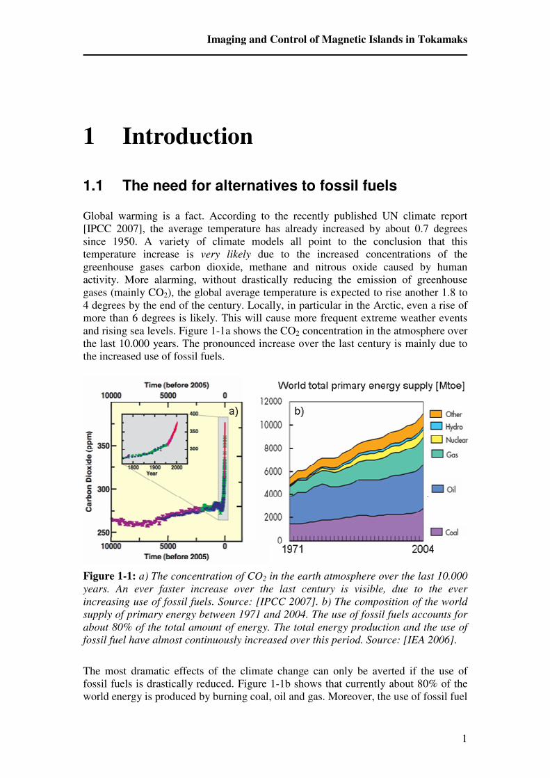
and rising sea levels. Figure 1-1a shows the CO2 concentration in the atmosphere over
the last 10.000 years. The pronounced increase over the last century is mainly due to
the increased use of fossil fuels.
Figure 1-1: a) The concentration of CO2 in the earth atmosphere over the last 10.000
years. An ever faster increase over the last century is visible, due to the ever
increasing use of fossil fuels. Source: [IPCC 2007]. b) The composition of the world
supply of primary energy between 1971 and 2004. The use of fossil fuels accounts for
about 80% of the total amount of energy. The total energy production and the use of
fossil fuel have almost continuously increased over this period. Source: [IEA 2006].
The most dramatic effects of the climate change can only be averted if the use of
fossil fuels is drastically reduced. Figure 1-1b shows that currently about 80% of the
world energy is produced by burning coal, oil and gas. Moreover, the use of fossil fuel

1 Introduction
2
has almost doubled over the period 1971-2004, and is still growing. To change this
trend, the development of (CO2-free) alternative energy sources is needed.
An equally important argument for developing alternative energy sources is the
limited reserve of fossil fuels. Although there is still a large coal reserve, oil and gas
are expected to become scarce over the course of this century. Sooner or later, the
ever scarcer supply of fossil fuels will no longer balance against the ever increasing
energy demand. If by that time no alternatives are available, this will be devastating
for the world economy.
Examples of currently available renewable (so, practically inexhaustible and
environmentally friendly) energy sources are bio, hydro, geothermal, wind and solar
energy. These are currently responsible for respectively 3.6, 2.2, 0.4, 0.05 and 0.04
percent of the world energy production [IEA 2003]. For large-scale CO2-free energy
generation, only four options are presently known of. These are nuclear fission, solar
power, carbon sequestration (so burning fossil fuels, but capturing the emitted CO2)
and fusion [Llewellyn-Smith 2005]. To develop a sustainable energy infrastructure,
all four options are needed as fast as possible. Fusion would be a practically
inexhaustible and safe source of energy. Moreover, fusion is CO2-free and the fuels
can not be used for the production of nuclear weapons. Although fusion will produce
a limited amount of radioactive waste products, these are contaminated only for a
short period of time (50-100 years).
The social acceptance of nuclear fission is variable but low in a number of countries.
This is mainly due to accidents that happened (Chernobyl), the long-lived nuclear
waste and the proliferation of fissile material. Moreover, the reserves of fission fuel
are limited, too. Some of these problems could be overcome with modern reactor
designs and fuel cycles, but these are not yet ready for large-scale implementation.
Fission could, however, be used to bridge the period between losing the fossil fuels
and the installation of a sufficiently large renewable energy infrastructure.
In the long term energy mix, nuclear fusion could play a large role. Fusion has very
attractive characteristics as a energy source, but it has one drawback: it is an
extremely difficult technology. Fifty years of fusion research has given a very rapid
progress, though. The figure of merit of fusion reactors, the power multiplication
factor (equivalent Q), was doubled every 1.8 years over a period of 40 years, reaching
unity in the present generation of large fusion test reactors such as JET. The world-
wide collaborative fusion test reactor ITER, of which construction is starting in
Cadarache (France), is designed to produce 500 MW of fusion power, ten times more
than the power needed to sustain the reaction.
1.2 Nuclear fusion and the tokamak concept
A chemical process, like the burning of oil, taps its energy [typically in the order of an
electronvolt (1 eV = 1.6.10
-19J) per reaction] from the binding energy of the electrons.
Nuclear fission and fusion tap their energy from the binding energy of nucleons
(protons and neutrons) inside the atomic cores (typically in the order of a MeV per
reaction). Iron has the strongest bound nucleus, and is hence in the most favourable
energy state. By splitting larger (fission), or merging smaller (fusion) nuclei, resulting

Imaging and Control of Magnetic Islands in Tokamaks
3
in more iron-like reaction products, energy is released. For nuclear fusion, the reaction
between the hydrogen isotopes deuterium ( HD21= ) and tritium ( HT
31= ) is foreseen,
resulting in helium and a neutron. In this reaction 17.6MeV of energy is released,
mainly (14.1MeV) as kinetic energy of the lighter neutron.
Eq. 1-1
Although this reaction is exothermic, it does not happen spontaneously. The two
positively charged D and T nuclei repel each other due to the Coulomb force. One
way to overcome this barrier is to raise the temperature of the reacting gases, so that
their thermal energy is sufficient to overcome the Coulomb barrier. For the D-T
reaction, the temperature needed is about 10 keV (as a measure of temperature,
1eV=11600K, so 10keV is more than 100 million K!). At such high temperatures,
electrons can no longer be bound to the atoms. The resulting ‘gas’ of free electrons
and stripped nuclei is called a plasma.
Contrary to a gas, where all particles are electrically neutral, a plasma responds to a
magnetic field. For charged particles, motion parallel to the field lines is unrestricted,
while perpendicular motion results in a gyration with (cyclotron) frequency
meBc =ω and (Larmor) radius cL v ωρ ⊥= .This can be used to confine the plasma.
Confinement is the ability to keep energy and particles in the plasma, and hence to
limit the outward energy and particle fluxes. A high confinement is absolutely
necessary for a fusion plasma to efficiently reach the required high temperature and
density.
To date, the best confinement has been achieved by a magnetic configuration called
the tokamak. A toroidal vacuum vessel contains the plasma, see Figure 1-2. This
plasma is confined by both a toroidal Bφ and a poloidal magnetic field Bθ, giving a
resultant helical field. The toroidal field is produced by external coils, the poloidal
field by a current in the plasma. This plasma current is produced by making the
plasma the secondary winding of a transformer. The poloidal field (so the plasma
current) is necessary to avoid the loss of the plasma due to curvature B and B∇ drifts,
occurring if only a toroidal field is present. The plasma current also heats the plasma.
Additional heating can be applied by injecting high-energy particles (NBI, Neutral
Beam Injection) or through the resonant absorption of electromagnetic radiation
(ICRH or ECRH, Ion or Electron Cyclotron Resonance Heating).
Current tokamaks (like TEXTOR) are too small to have a positive energy balance, so
more energy has to be put in than fusion energy is produced. However, the energy
balance improves with the size of a tokamak. The future ITER tokamak (R0=6.2m
a=2m), being build in southern France, is the first tokamak designed to produce
significantly (10 times) more energy than has to be put in.
Although the tokamak has proven to be successful in confining a fusion plasma, and
our understanding of tokamak plasmas enables a quite accurate prediction of the
performance of ITER, many questions remain. In this thesis we focus on phenomena
leading to an enhanced loss of energy and particles from the plasma. In particular, the
unwanted, spontaneous occurrence of magnetic field disturbances, the so called
magnetic islands, is investigated.
MeVnHeTD 6.1742 ++→+

1 Introduction
4
Figure 1-2: Schematic representation of a tokamak, showing the main constituents:
the toroidal-field coils, the transformer to induce the plasma current and the resulting
field components. Also, the major radius R0 and minor radius a are indicated.
1.3 Magnetic islands
The helicity of a field line can be expressed by the safety factor q, defined as the
number of toroidal turns needed to make one poloidal turn, and depends on the ratio
between the toroidal and poloidal magnetic fields. In a cylindrical plasma, q is
approximated by [Wesson 1997]
Eq. 1-2
For normal tokamak operation, the value of q increases with minor radius, being about
1 at the magnetic axis and 2-10 (depending on total plasma current) at the edge. A
rational q surface is a flux surface where q can be written as q=m/n, m and n being the
(natural) poloidal and toroidal mode numbers. At such a rational q surface, the
individual field lines close on themselves after m toroidal turns.
Ideally, in a tokamak the helical field lines define a set of nested flux surfaces, see
Figure 1-3a. Outward (so radial) heat and particle transport is then only possible
perpendicular to the field lines, for instance by collisions. In reality, however, a
variety of instabilities can lead to less ideal magnetic topologies.
One of the most common instabilities is the tearing mode or magnetic island.
Magnetic islands occur at rational q surfaces. The presence of a perturbed radial
magnetic field with a Fourier component resonant with the q=m/n surface results in
the formation of a magnetic island in the magnetic field topology. A magnetic island
θ
φ
BR
rBq
0
=

Imaging and Control of Magnetic Islands in Tokamaks
5
can be seen as a closed, helical flux tube, with helicity m/n, meaning it closes on itself
after going m times around the torus, while going n times around poloidally. Figure
1-3b shows the non-axisymmetric flux surfaces in the presence of magnetic islands (in
this case both a m/n=1/1 and a 2/1 island). The original q=m/n surface, now forms the
boundary of the island flux tube and is called the island separatrix, with its typical X-
point in the poloidal cross section. The magnetic axis of the island flux tube is called
the O-point. Magnetic islands (so a radial magnetic perturbation) develop either due to
the introduction of an external resonant magnetic perturbation field, or by a
(energetically favourable) non-axisymmetric redistribution of the plasma current.
a) b)X-point
O-point
a) b)a) b)X-point
O-point
Figure 1-3: Magnetic field topology in a) the ideal case, with nested flux surfaces,
and b) in the presence of magnetic islands. Both an m/n=1/1 and a 2/1 island are
shown. The X and O-points of the 2/1 island are indicated.
Although tokamak operation is possible with (not too large, saturated) magnetic
islands, they do have a deleterious effect on the confinement. The island flux surfaces
make radial excursions, offering a shortcut along the field lines for radial transport.
This results in flattened temperature and density profiles over the island region.
In larger tokamaks, like the future ITER tokamak, a type of magnetic island called the
neoclassical tearing mode (NTM) will pose a limit on the parameter range for efficient
operation. This mode is destabilised by the loss of bootstrap current (which is a
thermo-electric current driven by the density gradient) inside the island, due to the
flattened pressure profile. As the bootstrap current depends on the ratio between the
plasma pressure and the poloidal magnetic pressure (βθ), NTMs occur in high
performance (high pressure) plasmas.
Also, magnetic islands play an important role in disruptions. A (major) disruption is a
fast, total loss of confinement, terminating the plasma. The resulting large forces and
heat loads on the walls make a disruption an unwanted event that may even lead to
damage to the reactor. Normally, magnetic islands rotate with the same velocity as the
electrons. Disruptions can occur when a magnetic island locks to the static error field.
In that case the mode comes to a standstill, and grows rapidly. Small error fields are
present in all tokamaks, for instance due to a slight coil misalignment. Also a locking
(and subsequent growth) of two island chains can lead to a loss of the plasma.

1 Introduction
6
In summary, the presence of magnetic islands deteriorates the confinement of a
plasma, and makes it more susceptible to disruptions. Hence, magnetic islands should
generally be avoided. The control of magnetic islands is the main subject of this
thesis. To control islands, both a good knowledge of the theory of island evolution,
and tools to influence this evolution are needed. To compare experiment with theory,
diagnostics measuring the key parameters are needed.
1.4 This thesis
The theory of magnetic islands is known to a large extent. The evolution of the island
width is described by the (modified) Rutherford equation, relating island growth to the
various sources of helical current in the island region. Each current source is
represented by a different term in the Rutherford equation, and represents a way to
control (normally suppress) magnetic islands. This thesis focuses on the experimental
verification of two terms in the Rutherford equation that are normally difficult to
evaluate; the heating term and the perturbation field term. On TEXTOR, the
combination of available tools puts us in a unique situation to study these two terms.
The three main tools used in this thesis are:
• The electron temperature diagnostic ECE-Imaging (Electron Cyclotron Emission
Imaging) [Park 2003] to visualize magnetic islands in 2D with a high spatial and
temporal resolution.
• The Dynamic Ergodic Divertor (DED), to generate magnetic islands in a very
controlled way by applying a perturbation field of known amplitude and phase
[Special Issue 1997].
• A 140 GHz gyrotron [Westerhof 2003] to locally heat magnetic islands by
Electron Cyclotron Resonance Heating (ECRH) or drive current by Electron
Cyclotron Current Drive (ECCD).
ECE-Imaging enables the accurate measurement of the island width, phase and
temperature profile. The island width and phase are important parameters in the
theory of the interaction of islands with a perturbation field. The island width and
temperature profile are the main parameters for the theory of island suppression by
heating. The experiments on magnetic islands are presented in chapters 8 and 9.
Before coming to the core of the thesis, however, first the capabilities of the ECE-
Imaging diagnostic are explored in chapters 5 and 6. In these chapters ECE-Imaging
will be used to study two phenomena that are, like magnetic islands, (thought)
responsible for enhanced transport: A perturbed magnetic field at the plasma edge to
purposely enhance the edge transport, and high frequency fluctuations thought
responsible for the anomalously high transport observed in tokamaks. In these
chapters, ECE-Imaging and (in chapter 5) the DED are the main tools used.
In chapter 5, the 2D nature of the ECE-Imaging measurements is exploited in
measurements at the plasma edge during DED operation. Apart from a tool to
investigate magnetic islands, the DED was designed to alter the edge transport
properties. During DED operation, the plasma edge shows a pronounced 2D structure,
caused by field lines intersecting the wall. This chapter tries to find answers to the
questions:

Imaging and Control of Magnetic Islands in Tokamaks
7
• What is the effect of the DED perturbation field on the 2D edge temperature
profile?
• How does the transport at the edge change during DED operation?
• Can the DED be used to influence the plasma surface interaction?
In chapter 6, the possibilities of measuring high frequency fluctuations with ECE-
Imaging are investigated. In principle, ECE-Imaging is capable of measuring high
frequency fluctuations with a high spatial resolution, using correlation to suppress the
thermal noise inherent to all ECE diagnostics. This chapter tries to find answers to the
questions:
• Is ECE-Imaging indeed capable of detecting fluctuation with amplitudes far below
the noise level, as expected when using correlation techniques?
• Which types of fluctuations can we see at TEXTOR, and what properties do they
have?
• Can we see the fluctuations generally thought responsible for the experimentally
observed high transport levels?
After having explored the capabilities of ECE-Imaging, the main subject of this thesis,
magnetic islands, is treated in chapters 8 and 9. But before that, the procedure to
experimentally determine the island parameters is developed in chapter 7.
In chapter 8, experiments are described investigating the interaction of magnetic
islands with perturbation fields. Theoretically, the occurrence of a shielding current
results in the processes of mode penetration and mode unlocking. ECE-Imaging is
able to measure two parameters playing an important role in theory: the island width
and the phase difference between the island and the field perturbation. The known and
controllable perturbation field of the DED and ECE-Imaging are used to answer the
following questions:
• Are mode penetration and unlocking observed in the experiment, and are the
thresholds in accordance with theory?
• Is the island growth after penetration in accordance with the Rutherford equation?
• Can we see and understand (changes in) the expected phase difference between
the perturbation field and the actual island?
In chapter 9, DED induced islands are locally heated with ECRH to suppress them.
The resulting temperature peaking and suppression rate is measured with ECE-
Imaging and compared with theory to answer the following main questions:
• Is the energy confinement inside magnetic islands high enough to maintain a large
enough temperature peaking?
• Is the expected suppression of magnetic islands due to this peaked temperature
actually observed?
• Is suppression by heating of importance for the suppression of NTMs in a reactor?
Before describing the experimental results, in chapter 2 the theory of (the evolution
of) magnetic islands is given. The ‘hardware’ used in this Thesis (TEXTOR, DED,
diagnostics) is described in chapter 3. Finally, the theory of ECE as a temperature
diagnostic is treated in chapter 4, along with the description of the ECE-Imaging
system.

1 Introduction
8
1.5 List of publications
Below is a list of publications related to my work on TEXTOR. Publications directly
related to this thesis are marked with an asterisk (*).
• Journal publications
*I.G.J. Classen, E. Westerhof, C.W. Domier, A.J.H. Donné, R.J.E. Jaspers, N.C.
Luhmann Jr., H.K. Park, M.J. van de Pol, G.W. Spakman, M.W. Jakubowski and
TEXTOR team,
‘Effect of heating on the suppression of tearing modes in tokamaks’,
Physical Review letters 98, 35001 (2007)
*I.G.J. Classen, R.J.E. Jaspers, H.K. Park, G.W. Spakman, M.J. van de Pol, C.W.
Domier, A.J.H. Donné, N.C. Luhmann Jr., E. Westerhof and TEXTOR team,
‘Imaging meso-scale structures in TEXTOR with 2D-ECE’,
accepted for publication: Japan Journal: Plasma and Fusion Research
*I.G.J. Classen, M.F.M. de Bock et al.,
‘Dynamics of tearing modes in the presence of a perturbation field’
submitted to Nuclear Fusion
*M.F.M. de Bock, I.G.J. Classen et al.,
‘The interaction between plasma rotation, stochastic fields and tearing mode
excitation by external perturbation fields’
submitted to Nuclear Fusion
*E.Westerhof, A. Lazaros, E. Farshi, M.R. de Baar, M.F.M. de Bock, I.G.J. Classen,
R.J.E. Jaspers, G.M.D. Hogeweij, H.R. Koslowski, A. Krämer-Flecken, Y. Liang, N.J.
Lopes Cardozo and O. Zimmermann,
‘Tearing mode stabilization by electron cyclotron resonance heating demonstrated in
the TEXTOR tokamak and the implication for ITER’,
Nuclear Fusion 47 85 (2007)
H.K. Park, N.C. Luhmann, A.J.H. Donné, I.G.J. Classen, C.W. Domier, E.
Mazzucato, T. Munsat, M.J. van de Pol, Z. Xia and TEXTOR team,
‘Observation of high-field-side crash and heat transfer during sawtooth oscillation in
magnetically confined plasmas’,
Physical Review Letters 96, 195003 (2006)
H.K. Park, A.J.H. Donné, N.C. Luhmann, I.G.J. Classen, C.W. Domier, E.
Mazzucato, T. Munsat, M.J. van de Pol, Z. Xia and TEXTOR team,
‘Comparison study of 2D images of temperature fluctuations during sawtooth
oscillation with theoretical models’,
Physical Review Letters 96, 195004 (2006)

Imaging and Control of Magnetic Islands in Tokamaks
9
H.K. Park, E. Mazzucato, N.C. Luhmann, C.W. Domier, Z. Xia, T. Munsat, A.J.H.
Donné, I.G.J. Classen, M.J. van de Pol and TEXTOR team,
‘Self-organized T-e redistribution during driven reconnection processes in high-
temperature plasmas’,
Physics of Plasmas 13, 055907 (2006)
B.P. van Milligen, I.G.J. Classen, C.J. Barth,
‘Revision of TV Thomson scattering data analysis and detection of profile structure’
Review of Scientific Instruments 74 3998 (2003)
N.J. Lopes Cardozo, I.G.J. Classen, C.J. Barth, C.C. Chu, A.J.H. Donné, R. Jaspers, J.
Lok, A.A.M. Oomens, F.J. Pijper, F.C. Schuller,
‘Erratum: Plasma filamentation in the Rijnhuizen tokamak RTP’
Physical Review Letters 90, 149901 (2003)
*H.R. Koslowski, E. Westerhof, M. de Bock, I. Classen, R. Jaspers, Y. Kikuchi, A.
Kramer-Flecken, A. Lazaros, Y. Liang, K. Lowenbruck, S. Varshney, M. von
Hellermann, R. Wolf, O. Zimmermann, and TEXTOR team,
‘Tearing mode physics studies applying the dynamic ergodic divertor on TEXTOR’,
Plasma Physics and Controlled Fusion 48, B53 (2006)
*K.H. Finken, S. Abdullaev, W. Biel, M.F.M. de Bock, S. Brezinsek, C. Busch, I.
Classen et al.,
‘Overview of experiments with the dynamic ergodic divertor on TEXTOR’,
Contributions to Plasma Physics 46, 515 (2006).
*M. Lehnen, S. Abdullaev, W. Biel, M.F.M. de Bock, S. Brezinsek, C. Busch, I.
Classen et al.,
‘Transport and divertor properties of the dynamic ergodic divertor’,
Plasma Physics and Controlled Fusion 47 B237 (2005)
K.H. Finken, S.S. Abdullaev, W. Biel et al., among them I.G.J. Classen,
‘The dynamic ergodic divertor in the TEXTOR tokamak: plasma response to dynamic
helical magnetic field perturbations’
Plasma Physics and Controlled Fusion 46, B143 (2004)
C.W. Domier, Z.G. Xia, P. Zhang, N.C. Luhmann, H.K. Park, E. Mazzucato, M.J. van
de Pol, I.G.J. Classen, A.J.H. Donné, R. Jaspers,
‘Upgrades to the TEXTOR electron cyclotron emission imaging diagnostic’,
Review of Scientific Instruments 77, 10E924 (2006)
*T. Munsat, E. Mazzucato, H. Park, C.W. Domier, M. Johnson, N.C. Luhmann, J.
Wang, Z. Xia, I.G.J. Classen, A.J.H. Donné, M.J. van de Pol,
‘2D imaging of electron temperature in tokamak plasmas’,
IEEE Transactions on Plasma Science 33, 466 (2005)
A.J.H. Donné, M.F.M. De Bock, I.G.J. Classen et al.,
‘Overview of core diagnostics for TEXTOR’,
Fusion Science and Technology 47, 220 (2005)

1 Introduction
10
*H. Park, E. Mazzucato, T. Munsat, C.W. Domier, M. Johnson, N.C. Luhmann, J.
Wang, Z. Xia, I.G.J. Classen, A.J.H. Donne, M.J. van de Pol,
‘Simultaneous microwave imaging system for density and temperature fluctuation
measurements on TEXTOR’,
Review of Scientific Instruments 75, 3787 (2004)
*J. Wang, C.W. Domier, Z.G. Xia, Y. Liang, N.C. Luhmann, H. Park, T. Munsat, E.
Mazzucato, M.J. van de Pol, I.G.J. Classen, A.J.H. Donné,
‘Two-dimensional electron cyclotron emission imaging diagnostic for TEXTOR’,
Review of Scientific Instruments 75, 3875 (2004)
• Conference contributions
*I.G.J. Classen, E. Westerhof, C.W. Domier, A.J.H. Donné, R. Jaspers, N.C.
Luhmann Jr., J.W. Oosterbeek, H.K. Park, M.J. van de Pol, G.W. Spakman and
TEXTOR team,
‘2D ECE Temperature Measurements Inside Tearing Modes, Revealing the
Suppression Mechanism by ECRH at TEXTOR’,
Invited Oral: In proceedings of the 14th
Joint Workshop on Electron Cyclotron
Emission and Electron Cyclotron Resonance Heating (EC-14), Santorini, p134 (2006)
*I.G.J. Classen, M.J. van de Pol, S. Leerink, A.J.H. Donné, C.W. Domier, N.C.
Luhmann, Jr., E. Mazzucato, T. Munsat,H.K. Park, and the TEXTOR team,
‘ECE correlation measurements of electron temperature fluctuations on TEXTOR
using the new 2D ECE-imaging diagnostic’,
In proceedings of the 13th
Joint Workshop on Electron Cyclotron Emission and
Electron Cyclotron Resonance Heating (EC-14), Nizhny Novgorod, p108 (2005)
I.G.J. Classen, S.K. Varshney, C.J. Barth and the TEXTOR team,
‘Improved analysis of TEXTOR Thomson Scattering data, taking account of the
effects of the Instrument Function’
30th
EPS conf. on Contr. Fusion and Plasma Physics, St. Petersburg P-2.132 (2003)
*I.G.J. Classen, M.J. van de Pol, S. Leerink, A.J.H. Donné, C.W. Domier, N.C.
Luhmann Jr., E. Mazzucato, T. Munsat, H. Park, A. Krämer-Flecken and TEXTOR
team,
‘Fluctuation measurements with the 2D ECE Imaging system on TEXTOR’
31st EPS conference on Contr. Fusion and Plasma Physics, London P-1.121 (2004)
*I.G.J. Classen, M.W. Jakubowski, A.J.H. Donné, M.J. van de Pol, C.W. Domier,
H.K. Park and TEXTOR team,
‘2D temperature profiles of DED structures using ECE-Imaging in TEXTOR’,
32nd
EPS conference on Contr. Fusion and Plasma Physics, Tarragona P-2.041 (2005)
*I.G.J. Classen, E. Westerhof, C.W. Domier, A.J.H. Donné, R. Jaspers, N.C.
Luhmann Jr., J.W. Oosterbeek, H.K. Park, M.J. van de Pol, G.W. Spakman and
TEXTOR team4
‘2D ECE Temperature Measurements inside Tearing Modes, Revealing the
Suppression Mechanism by ECRH at TEXTOR’,
33rd
EPS conference on Contr. Fusion and Plasma Physics, Rome P2.169 (2006)

Imaging and Control of Magnetic Islands in Tokamaks
11
2 The theory of magnetic islands
Most of this thesis deals with magnetic islands (or more formally: tearing modes). In
chapter 8, experiments will be described in which islands will be created using
perturbation fields. In chapter 9, local heating by ECRH will be used to suppress
them. Magnetic islands are one of the most common instabilities in a tokamak plasma.
Larger magnetic islands have a negative effect on the ability of a plasma to confine
energy and particles, and should hence generally be avoided. Very large islands (or
the simultaneous occurrence of more than one island) can even lead to a rapid loss of
the confinement in a so called disruption.
In this chapter the theory of magnetic islands is reviewed. The emphasis lies on the
effects leading to a growth or a suppression of magnetic islands. The evolution of the
island width, described in a modified version of the Rutherford equation, is mainly
determined by the various parallel currents that are present in the island region. Each
type of current corresponds to a different mechanism that can be used to suppress or
destabilize magnetic islands. In particular the effects of external perturbation fields
(described in [Fitzpatrick 1993/95/98]) and local heating are important for this thesis.
For some equations, in particular for those concerning torques, the sign is important.
As this depends on the definition of the coordinate system, Figure 2-1 shows the right
handed (r,φ,θ) coordinate system used throughout this thesis.
rφ
θ
B
fe*
NBI
Ip
rφ
θ
B
fe*
NBI
Ip
Figure 2-1: The definition of the (r,φ,θ) coordinate system. The directions of the
magnetic field, co-NBI injection and diamagnetic drift are indicated for a normal
TEXTOR discharge.
2 The theory of magnetic islands
12
2.1 The island topology
Magnetic islands form when a perturbed radial magnetic field with a certain mode
structure (m,n) is present, on top of the equilibrium magnetic field (whose radial
component is zero, for simplicity assuming the equilibrium flux surfaces to be
perfectly circular). In the presence of this perturbed field, the ideal magnetic topology
of nested flux surfaces breaks down and the typical island structure forms on the
q=m/n resonant surface. An island can be seen as a closed helical flux tube, closing on
itself after going m times around the torus while going n times around poloidally. The
island flux tube is bounded by the separatrix, with its typical X-point in the poloidal
cross section. The O-point is the magnetic axis of the island flux tube. Individual field
lines in the island make large radial excursions, offering a shortcut for the radial
transport of energy and particles. To compare, a typical large island in TEXTOR has a
width w of about 10cm, which is much larger than the typical gyro-radii ρe=0.05mm
and ρi=2mm (which are the step sizes for classical, collisional transport).
The radial excursion of a field line caused by the perturbed m/n radial magnetic field
is negligible unless the field line lies close to the rational q surface q=m/n, resonant
with the perturbation. It is common to introduce a new (helical) coordinate
Eq. 2-1
which is directed perpendicular to the equilibrium field lines at the m/n surface. The
perturbed radial magnetic field can then be written as
Eq. 2-2
where ω is the mode frequency. The resulting island topology (for positive dq/dr,
assumed throughout this chapter), which is a superposition of the perturbed radial
field Br and the equilibrium field, is given by ([Fitzpatrick 1993],[Hegna
1997],[Wilson 2004])
Eq. 2-3
Eq. 2-4
where y = r-rs is the radial distance to the rational q=m/n surface at minor radius rs, w
is the full island width and Ω is a label of the perturbed flux surfaces acting as a radial
coordinate inside the island, ranging from -1 at the O-point, to +1 at the separatrix. At
t=0 (assumed throughout this chapter), the O-points of the island chain are located at
mξ=0 mod(2π). Figure 2-2 shows the geometry given by Eq. 2-3 for a 2/1 island in the
ξ-y plane. Note that only the component of the equilibrium field in this ξ-y plane (B*)
plays a role in the construction of the island. Due to the (assumed constant) magnetic
shear, B* (which is in the ξ-direction) changes linear with y and changes sign over the
resonant surface (where it is zero). The lines, representing flux surfaces, are contour
φθξm
n−=
)sin()(r,0r tmrBB ωξ −=
)cos(22
tmw
y ωξ −+Ω=
drdqmB
rqBw
/4
θ
r,0=

Imaging and Control of Magnetic Islands in Tokamaks
13
lines of Ω. Note that already very small radial field perturbations lead to considerable
island sizes. For typical TEXTOR parameters (Bφ=2.25T, q=m=2, dq/dr=6), already
φBBr4
0, 10−= gives a m/n=2/1 island with w=3cm.
Figure 2-2: Contour plot of Ω for a m/n=2/1 island in the ξ-y plane. The O-point, the
X-point and the (full) island width w are indicated. The separatrix is shown as a thick
black line.
It should be noted that Figure 2-2 only represents the flux surfaces, not the magnetic
field lines themselves. The (in this case) m/n=2/1 component of the magnetic field
lines (directed ‘into the paper’) is much larger than the component perpendicular to
the 2/1 component (in the plane of the figure). So in reality the magnetic field lines
deviate only slightly from the unperturbed topology. For a particle gyrating around
and travelling along these field lines the island structure only becomes apparent after
travelling a long way along the field line, many times around the torus. Here, a second
winding number qtm=mtm/ntm can be introduced describing the helicity of the field
lines inside the island with respect to magnetic axis of the island (so the O-point). The
field lines inside the island rotate ntm times around the O-point after travelling mtm
times around the torus, whereas the island flux tube as a whole has a (normal) q=m/n
structure. Close to the island separatrix, qtm goes to infinity.
Instead of the perturbed poloidal magnetic field ( B~
, with radial component Br), it is
practical to use the perturbed poloidal flux function ψ (in units of Tm2), defined as
1
Eq. 2-5
Assuming the perturbed flux to have the form
Eq. 2-6
1 In literature (in particular in the often referred to articles of Fitzpatrick), often a slightly different
definition for the poloidal flux function is encountered which has units of [Tm], defined by
ψ∇×= zB ˆ~
, where z is the unit vector in toroidal direction. One can convert this definition to the
one used in this thesis by simply multiplying by R0.
ψφ ∇×∇=B~
)cos(0 tm ωξψψ −=

2 The theory of magnetic islands
14
gives a perturbed poloidal magnetic field in radial direction:
Eq. 2-7
where ψ0 has been assumed constant over the island region. This so called ‘constant
ψ approximation’, already used in the derivation of Eq. 2-3, is common in literature
and results in symmetric islands. From Eq. 2-4 and Eq. 2-7 follows the relationship
between the amplitude of the perturbed flux ψ0 and the full island width w:
Eq. 2-8
where the proportionality constant C, containing the equilibrium parameters, is
introduced.
2.2 The effect of an island on Te and ne
Whether a magnetic island has a large effect on the profiles of electron temperature Te
and density ne depends on the ratio between perpendicular and parallel transport. Due
to the fact that parallel transport is orders of magnitude larger then perpendicular
transport, Te and ne can normally be assumed flux functions. Any gradient parallel to a
flux surface is quickly removed by the large parallel transport. For a magnetic island,
this would mean that the inner and outer separatrix have equal Te and ne, and (in the
absence of significant heat sources or sinks inside the separatrix) that the profiles
inside the separatrix are flat. Parallel transport offers a radial shortcut for the transport
of energy and particles over the island. The assumption that Te and ne (and hence also
the pressure p) are flux functions is justified on all flux surfaces where the transport
from one location on that surface to another is dominated by parallel transport. This
is, however, not the case on (flux surfaces close to) the separatrix, where the
individual field lines have (almost) the same helicity as the island itself. After m
toroidal turns, a field line on the separatrix gets back to its starting point. Moreover, as
the local island winding number qtm approaches infinity the field line has not made
any radial excursion during these m turns. As a result of this ‘field line stagnation’,
transport from one location on the separatrix to another is only possible through
perpendicular transport. For flux surfaces close to the separatrix, a large number of
toroidal turn is needed for an individual field line to ‘migrate’ from one location on
that flux surface to another. So, although the transport parallel to these field lines is
orders of magnitude larger than the perpendicular transport, also the parallel distance
connecting two points on their flux surfaces is orders of magnitude larger than the
perpendicular distance. So on flux surfaces close to the separatrix, the parallel and
perpendicular transport channels compete, making gradients parallel to the flux
surfaces possible.
A consequence of this conclusion, drawn from transport arguments, is that in the
vicinity of the island separatrix, the standard MHD momentum equation pBj ∇=× ,
implying the absence of a pressure gradient parallel to B, is no longer completely
valid, although the deviations are very small because the component of B parallel to
22
2
s2
θ
016
d
d
16
d
d
Cwwq
r
qBr
wq
Rr
qB
≡==φ
ψ
rR
mB 0
r,0
ψ=
Imaging and Control of Magnetic Islands in Tokamaks
15
the pressure gradient is very small (even zero at the separatrix). A more general form
of the momentum equation is given by [Friedberg 1987]:
Eq. 2-9
where ∇⋅+∂∂= vtdtd // represents the convective derivative and ΠΠΠΠj is the
anisotropic pressure tensor, mainly including viscosity. So either the right hand side
of this equation, or the inertial term on the left hand side, can cause (small) parallel
pressure gradients. In MHD theory, the right hand side is neglected as it is assumed
that the pressure is always equilibrated (isotropic). Close to the island separatrix,
however, the very long connection length between different points on the flux
surfaces results in long pressure equilibration times [Milligen 1993][Hegna 1998]
(going to infinity at the separatrix itself), making the assumption of equilibrated
pressure difficult to hold.
The equilibration of Te along a field line can be described by writing the electron heat
flow as
Eq. 2-10
where qe is the electron heat flux, een χκ = is the thermal conductivity (χe is the
electron heat diffusivity) and the subscripts // and ⊥ respectively denote the parallel
and perpendicular components. Solving Eq. 2-10 around a magnetic island, a critical
island width wc,T can be found [Fitzpatrick 1995], below which the parallel transport
can not guarantee Te to be a flux function:
Eq. 2-11
where dr
dq
q
rss = is the local magnetic shear. Analogously, for ne a critical island
width wc,n is found by replacing the thermal conductivities by the particle diffusion
coefficients D:
Eq. 2-12
This critical width for ne is typically a few times larger than the one for Te (In
[Fitzpatrick 1995] a factor 3.9 is mentioned), mainly due to the smaller parallel
transport. When a magnetic island is much smaller than these critical widths, no
significant flattening of the profiles occurs. The magnetic island, although present as a
magnetic perturbation, is hence not visible in the Te and ne profiles.
For islands larger than the critical widths, there exists a layer, centred on the
separatrix, where parallel gradients in ne and/or Te are possible, see Figure 2-3. The
width of this layer is largest, about wc, around the X-point. Half way between the X-
points its width is about wwc /2 . In the interior of the island, the profiles flatten if there
is no significant local heat or particle source. Heat or particle fluxes flowing across
the island (so radially out from the centre of the plasma towards the edge), do not
eee TTq ⊥⊥∇−∇−= κκ ////
2/1
0
4/1
//,
= ⊥
ns
rRw
s
sTc
κ
κ
2/1
0
4/1
//,
= ⊥
ns
rR
D
Dw
s
snc
)( eipBjdt
dvΠΠ +⋅−∇=∇+×−ρ

2 The theory of magnetic islands
16
enter the interior of the island, but are conveyed through the X-point by the parallel
gradients on the boundary layer.
Figure 2-3: The layer in which Te and ne can
not be considered flux functions. Islands
smaller than the critical width wc do not result
in significantly flattened profiles. This critical
island width is larger for ne as for Te. For
islands larger than wc, there is a layer around
the separatrix where parallel gradients of Te
and ne are possible. This layer, which channels
the heat flux across the island, is widest across
the X-point. Further inside the island, Te and
ne are flux functions. If there is no significant
heat source or sink inside this region, the
profiles are flat. In the presence of o local heat
source, this region (with its nested flux
surfaces) can confine heat and particles,
resulting in peaked profiles.
To find a quantitative value for the critical widths, the parallel and perpendicular
transport coefficients are needed. Perpendicular (anomalous) transport for both energy
and particles is comparable in amplitude and can be easily estimated from the energy
and particle confinement times. Various models for the parallel transport can be found
in literature ([Fitzpatrick 1995],[Hazeltine 1997],[Zohm 2001]), leading to a critical
island width wc,T of around 2cm for typical TEXTOR parameters.
2.3 The island evolution equation
The various types of currents in the plasma (and its boundary) all influence the
dynamics of magnetic islands. The natural stability of magnetic islands is determined
by the equilibrium toroidal current profile. The evolution of magnetic islands on the
other hand, is governed by the perturbed parallel helical currents in the island region.
Ampere’s law relates the second radial derivative of ψ to the parallel current density
j//:
Eq. 2-13
here the island is assumed to be small, so that, despite the change in the second radial
derivative, ψ itself changes only slightly over the island radius (constant ψ
assumption) Integrated over the (assumed narrow) island region, Eq. 2-13 gives the
basic equation for island evolution ([Rutherford 1973],[Hegna 1997],[Wilson 2004]):
Eq. 2-14
∫ ∫+
−
=∆′2/
2/
s//00
s
s
)cos(2
wr
wr
drmjdyR ξξµψ
//02
2
0 d
d1j
rRµ
ψ=
Imaging and Control of Magnetic Islands in Tokamaks
17
where the parameter ∆’ (‘delta prime’) is introduced:
Eq. 2-15
So ψ∆′ is the step in the radial derivative of ψ over the island region and is a direct
measure for the total perturbed parallel current in the island region. Notice that only
current distributions with a )cos( ξm component contribute to the integral (so the
equilibrium parallel current doesn’t contribute). The positive current direction is in the
direction of the equilibrium parallel current.
The value of ∆′ is a property of the plasma equilibrium (toroidal current profile) and
has to be evaluated by matching the ideal MHD solution of ψ for the region 0 < r <
(rs+w/2) to the solution for (rs-w/2) < r < ∞. This will generally give a jump in drd /ψ
at the rational surface.
Neglecting plasma flow and resistivity, a plasma in force balance obeys pBj ∇=× .
As the curl of a gradient equals zero, it follows that:
Eq. 2-16
Linearization of the perturbed toroidal component of this equation then gives the
differential equation governing the radial dependence of ψ ([Wesson 1997],
[Fitzpatrick 1993]):
Eq. 2-17
The step in ψ is found by integrating Eq. 2-17 (from the centre of the plasma outward,
and from ‘infinity’ inward to the resonant surface), using appropriate boundary
conditions [ ψ(0) = ψ(∞) = 0 ]. As the solutions to Eq. 2-17 are linear, it is only the
normalized step in the flux function (definition of ∆’) that is determined. So in
principle, ∆’ describes the matching criteria for magnetic islands of all sizes. Applied
in a region of the plasma where the toroidal current can be neglected (for instance
near the plasma edge), Eq. 2-17 predicts a perturbed flux function that falls of with m
srr−)/( for r>rs, and m
srr )/( for r<rs where rs is the radius of the current carrying
resonant surface. Notice that Eq. 2-17 has a singularity at the rational surface, as a
result of neglecting the resistivity. So, inside the island region, this equation is not
valid.
One can interpret ∆′ as a measure for the free energy available in the plasma to drive
a tearing mode. The change in magnetic energy in the presence of an island is given
by [Hegna 1994]:
Eq. 2-18
[ ] 2/
2/
r2/
2/
s
s
s
sd
ln(d
d
d1wr
wr
wr
wr r
rB
r
+
−
+
−
=
=∆′
ψ
ψ
0=××∇ Bj
0
1
d/d
d
d
d
d1
0
2
2
=
−
−− ψ
µ
ψψ
θ
φ
m
nqB
rj
r
m
rr
rr
∆′−= 204
1 ψδ smag rW

2 The theory of magnetic islands
18
So a positive ∆’ means that in the presence of an island, the plasma is in a lower
(more favorable) energy state.
2.3.1 The Rutherford equation
Equation Eq. 2-14 tells us how much current is flowing in the island, but doesn’t
directly reveal how an island evolves in time. This time evolution only becomes
apparent if we specify the mechanisms responsible for the perturbed parallel current.
One mechanism that is always present is the current that is induced by the time
derivative of ψ (and hence dw/dt) ([Hegna 1997],[Wilson 2004]):
Eq. 2-19
where η is the resistivity (at rs) and <> denotes an average over the helical flux
surfaces. If this induced current is the only current contributing to j//, equation Eq.
2-14 reduces to the classical Rutherford equation for island evolution [Rutherford
1973]:
Eq. 2-20
where τr = µ0rs2/η is the current diffusion time. So a positive ∆’ means a growing
island, as expected from the interpretation of ∆’ as the available free energy. If ∆’ is
negative, the island is naturally stable; no island will develop. For small islands
(w<<a) ∆’ is often considered independent of w, so the Rutherford equation predicts
unstable islands to grow exponentially. Bigger islands (w in the order of a)
considerably alter the toroidal current distribution, and hence a dependence of ∆’ on w
is expected (∆’ becoming smaller as the island grows; free energy is being used up).
This effect can be approximated by writing
Eq. 2-21
where wsat is the (experimentally determined) saturated island width. So the initially
linearly growing island finally saturates at width wsat when )(w∆′ =0.
A more precise derivation of the evolution equation, including the effects of plasma
flows, results in a slightly different form of the Rutherford equation [Wesson 1997]:
Eq. 2-22
where α is related to the local plasma parameters (∆’ per definition only contains
current profile effects). In the remainder of this thesis, when writing ∆’(w), actually
( )ww α−∆′ )( is meant.
)cos(1 0
// ξψ
ηm
tj growth
∂
∂=
∆′=⋅ 282.0 sr rdt
dwτ
−∆′=∆′
satw
ww 1)( 0
( )wwrdt
dwsr ατ −∆′=⋅ )(82.0 2

Imaging and Control of Magnetic Islands in Tokamaks
19
Introduction of other currents than the inductive current in the island region results in
modifications to the Rutherford equation. These are described in the next paragraph.
2.4 Other contributions to the helical current
The introduction of other currents (with a )cos( ξm component) in the island region
alters the evolution equation. A modified version of the Rutherford equation can be
found by substituting the sum of all contributions to j// into equation Eq. 2-14,
repeated here.
In general, extra current inside the island in the same direction as the equilibrium
parallel current (co-current) stabilizes the mode, and extra current in the other
direction is destabilizing. The total current in the island region is fixed by the left
hand side of Eq. 2-14, so extra current in the co-direction replaces the induced current
due to island growth. So due to the extra co-current, Eq. 2-14 can now be satisfied
without the need of island growth to maintain the prescribed total current.
The modifications to the island evolution equation due to the following extra (helical)
currents are treated in this paragraph:
• The perturbed bootstrap current, leading to neoclassical tearing modes
(NTMs).
• Shielding currents due to external perturbation fields.
• Currents caused by O-point heating.
• Currents due to direct non-inductive current drive
2.4.1 Perturbed bootstrap current: Neoclassical Tearing Modes
By introducing the perturbation in the bootstrap current due to the island, the
mechanism of the so called neoclassical tearing mode (NTM) becomes apparent. The
bootstrap current is a non-inductive current, which (in a simplified picture) is
proportional to the radial gradient in the plasma pressure [Wesson 1997]. Because
pressure is approximately a flux function for big enough islands [Fitzpatrick 1995],
the pressure gradient is effectively removed from the island region, leaving a ‘hole’ in
the bootstrap current profile with the necessary )cos( ξm component to influence the
island evolution. For negative dp/dr and positive dq/dr (true in common tokamak
regimes) this current perturbation opposes the induced current of the island, and hence
is destabilizing. So, even islands with a negative ∆’ can be destabilized. The inclusion
of the perturbed bootstrap current in Eq. 2-14 leads to a modified Rutherford equation
of the form [La Haye 2006]:
Eq. 2-23
∫ ∫+
−
=∆′2/
2/
s//00
s
s
)cos(2
wr
wr
drmjdyR ξξµψ
wL
LM
Mwrt
w
p
q
bootstrap
bootstrap
θβε
τ
2/1
2sr )(
d
d82.0
−≈
+∆′=
2 The theory of magnetic islands
20
where 0/ Rr=ε is the local inverse aspect ratio, )//( drdqqLq = the magnetic shear
length, )//( drdppLp = the pressure gradient length and 20 /2 θθ µβ Bp= the poloidal
β. Naturally stable (negative ∆’) islands destabilized by the perturbed bootstrap
current are called neoclassical tearing modes (NTMs).
If Eq. 2-23 would be the whole story, the w-1
dependence of Mbootstrap would always
destabilize an NTM. This would be catastrophic for the stable operation of tokamaks,
and is in contradiction with experimental findings. Experimentally, NTMs are only
destabilized above a certain threshold island width. So a ‘seeding’ island of sufficient
width is needed. Seeding islands can be provided by any (coincidental) distortion of
the plasma, for instance by the error field of a sawtooth precursor.
One correction on Eq. 2-23 is provided by the effects already described in paragraph
2.2. For small islands, temperature and density are not necessarily flux functions, and
hence the flattening of the pressure profile assumed in Eq. 2-23 does not occur.
Taking this effect into account results in [La Haye 2006]:
Eq. 2-24
where the critical width for pressure flattening wc is closely related to the ones for
temperature and density, Eq. 2-11 and Eq. 2-12.
A second effect leading to a threshold for island growth is the polarization current
correction [Waelbroeck 2001], resulting from a difference in response of electrons
and ions in a rotating island. This (complicated) correction results in a further ‘fine-
tuning’ of Mbootstrap:
Eq. 2-25
where the typical threshold island width due to the polarization current correction is
approximately given by
Eq. 2-26
where wb is the banana orbit width. This width also depends on collisionality and
island frequency.
With the inclusion of the threshold island widths in Mbootstrap, it now describes the
typical NTM behaviour. It should be noted that in TEXTOR the bootstrap current
fraction is generally small. TEXTOR magnetic islands are therefore generally of
classical origin (positive ∆’). TEXTOR, however, has a tool to destabilize otherwise
naturally stable tearing modes: the resonant perturbation field of the Dynamic Ergodic
Divertor, treated in the next paragraph.
22
2/1
c
pp
qbootstrap
ww
w
L
LM
+−≈ βε
−
+−≈
2
2
22
22/1
w
w
ww
w
w
r
L
LM
pol
c
sp
p
qbootstrap βε
bpqpol wLLw 2/1)/(≈

Imaging and Control of Magnetic Islands in Tokamaks
21
2.4.2 The effect of an external perturbation field
Resonant magnetic perturbation fields, generated by currents flowing outside the
island region, have a large influence on the stability of magnetic islands. On
TEXTOR, the Dynamic Ergodic Divertor (DED) is used to generate such a perturbed
field. In chapter 8, experiments investigating the effect of the DED field on magnetic
islands are presented.
Currents flowing in external coils generate a perturbation field with a certain mode
spectrum. This magnetic perturbation field can again be described by a perturbed
poloidal flux function. At the position of the external coils this flux function will have
a jump in the radial derivative, proportional to the current in the coils, analogous to
the jump in ψ at the resonant surface described in Eq. 2-14 and Eq. 2-15. In the
absence of a conducting plasma, this flux function will result in an island at the q=m/n
surface in the vacuum magnetic field (which is the superposition of the perturbation
field and the equilibrium field), with a width wvac and corresponding perturbed flux
)cos(0, tm extvacvac ωξψψ −= , where ωext is the mode frequency of the externally
applied field. The perturbed flux ψvac scales linearly with the external coil current
amplitude. The ideal MHD response of the plasma to this perturbed flux function will
be to generate a current at the rational surface that cancels the effect of the external
coil currents ([Fitzpatrick 1993],[Kikuchi 2006]). This shielding current has two
important effects: it alters the stability of m/n tearing modes, described by a modified
version of the Rutherford equation, and it exerts an electromagnetic torque on m/n
modes.
The modified version of the Rutherford equation is again found by including the
)cos( ξm component of the shielding current (expressed in terms of the vacuum island
width) in Eq. 2-14, leading to ([Fitzpatrick 1991], [Fitzpatrick 1993], [Fitzpatrick
1998], [Morris 1992a])
Eq. 2-27
where )()( ,, vacuumOplasmaOmm ξξξ −=∆ is the phase difference between the O-points
of the plasma island and the vacuum island. Notice that this modification is largest
when the plasma island is small, and when the island is aligned with the external
perturbation field (vacuum island).
The )sin( ξm component of the shielding current doesn’t influence the evolution of the
island width, but results in an electromagnetic torque TEM in the direction of ξ on the
island, trying to align the plasma island with the vacuum island. The origin of this
torque is the net Bj × force attributable to the shielding current and the radial
magnetic field of the island. The toroidal and poloidal components of this torque are
given by ([Fitzpatrick 1993], [Fitzpatrick 1998], [Fitzpatrick 1991]):
Eq. 2-28 ))(sin(4 222
00
2EMθ,EM, ξ
µπφ mwwC
R
mnT
m
nT vac ∆−=−=
))(cos(2
)(d
d82.0
2
vacs
2sR
ξ
τ
mw
wmrM
Mwrt
w
ext
ext
∆
=
+∆′=

2 The theory of magnetic islands
22
Because poloidal flow damping of the ions effectively prohibits any significant ion
rotation in poloidal direction [Stix 1973], only the toroidal component of this torque is
important.
If the MHD frequency ω is equal to the frequency of the externally applied
perturbation field ωext (as is the case for a locked island), Eq. 2-28 can be directly
applied. If, however, there is a difference in frequency, referred to as the ‘slip’
frequency
Eq. 2-29
one has to distinguish between two different cases, depending on the size of the
(induced) plasma islands. For both cases (referred to as the ‘non-linear’ and ‘linear’
cases), Eq. 2-28 is valid, but the expression for the time averaged electromagnetic
torque in terms of the slip frequency ∆ω, takes different forms.
2.4.2.1 The electromagnetic torque in the non-linear regime.
Large, ‘non-linear’, islands always rotate at the MHD frequency. The island is not
allowed to slip through the electron fluid. In this case, a non-zero ∆ω results in a
plasma island that is alternately dragged in and out of phase with the perturbation
field, giving a periodic growth and decay of the island and a fluctuating
electromagnetic torque. Assuming the island rotation is not significantly altered by the
fluctuating torque, and that the ∆’ term in the modified Rutherford equation (Eq. 2-27)
is negligible with respect to the large perturbation field term (which is the case for
small island widths), one can analytically solve the Rutherford equation, yielding the
fluctuating island width [Fitzpatrick 1998]
Eq. 2-30
where w0 is the maximum island size during one fluctuation. The time averaged
electromagnetic torque acting on the island in the non-linear regime can now (by
combining Eq. 2-30 and Eq. 2-28) be expressed as
Eq. 2-31
which is proportional to ∆ω-2/3 and in the direction to decrease ∆ω. Note that the ∆ω
dependence is hidden in w0.
2.4.2.2 The electromagnetic torque in the linear regime.
For very small islands, the island does not necessarily rotate at the same angular
velocity as the electron fluid, but slips through it to some extent. This effect is caused
by the viscosity between the island and the plasma ‘flowing around’ it. This viscosity
s
3/1
R
2s
2vac3/1
0
3/1
0
/939.1
)sin()(
rrw
mw
twtw
∆=
∆=
ωτ
ω
20
2vac
2
00
2
linearnonEM, 45356.0)( wwCR
mnsignT
µπωφ ⋅⋅∆−=
−
extωωω −=∆

Imaging and Control of Magnetic Islands in Tokamaks
23
arises in a thin layer (with thickness of the order of the linear layer mentioned in
[Fitzpatrick 1993], [Fitzpatrick 1998]), where an exchange of particles between the
island and the surrounding plasma occurs. The rotation frequency of ψ (so the
induced plasma island) can now slip with respect to the MHD frequency. In fact, ψ
will now rotate at the frequency of the external perturbation field, but with a phase
lag, resulting in a non-fluctuating torque and mode amplitude. For these experiments,
the linear layer is in the ‘visco-resistive’ regime treated in ([Fitzpatrick 1993],
[Fitzpatrick 1998]) (meaning that viscosity and resistivity are important, but inertia is
negligible, valid for 3/2R
3/2H
3/1V
−−<<∆ τττω ). The expression for the (visco-resistive)
linear layer width is given by:
Eq. 2-32
and is typically 3 mm in the experiments treated here. The hydromagnetic and viscous
time scales are given by
Eq. 2-33
where ρ is the plasma mass density ,D the effective momentum diffusion coefficient
and r
q
q
rs
d
d= the magnetic shear.
When the driven island width is larger than the linear layer width, the non-linear
description is appropriate. When however the island widths are comparable to, or
smaller than the linear layer width (as is usually the case during the early stages of
mode penetration), the following linear theory is needed.
In the visco-resistive limit, the steady torque, island width and phase lag are given by:
[Fitzpatrick 1993]
Eq. 2-34
Eq. 2-35
Eq. 2-36
where ∆0’ is the stability parameter at zero island width for the mode in question and
Eq. 2-37
s6/1V
6/1R
3/1H
VR rττ
τδ =
D
r
nsB
R
2s
V
0
φ
0H
=
=
τ
ρµτ
( )4vac
2
2rec
rec
s000
22
linearEM,,1
24 wC
rR
nmT
ωτ
ωτ
µπφ
∆+
∆
∆′−=
( )2vac
s02
rec
2 2
1
1w
r
mw
∆′∆+=
ωτ
)(tan)( rec1 ωτξ ∆=∆ −
m
6/1V
6/5R
3/1H
s0rec
1036.2
τ
τττ
r∆′=

2 The theory of magnetic islands
24
is the typical reconnection time scale in the visco-resistive limit. Figure 2-4 gives an
example of both the non-linear and linear theory for typical TEXTOR parameters. The
two theories are very similar (both showing the resonance at the perturbation field
frequency and similar torque amplitudes) despite the somewhat different parametric
dependencies. The fact that the curve for the linear theory passes through 0, and the
non-linear doesn’t, is due to the fact that in the non-linear curve ∆’ is fully neglected.
If a finite ∆’ would have been assumed, the resemblance between linear and non-
linear would have been even greater. The most important difference however, is that
the linear theory describes constant torques, whereas the non-linear theory deals with
oscillating torques.
Figure 2-4: Example of the electromagnetic torque, island width and phase difference
for both linear (solid) and non-linear (dashed) theory for typical TEXTOR
parameters, using the DED to create the perturbed field. The perturbation field
rotates at 1 kHz. The resonant character of the torque (trying to arrest the mode
rotation) is apparent. The induced island widths are only large when the mode
frequency is close to the perturbation field frequency. The phase difference is only
shown for the non-oscillating linear theory.
2.4.3 Heating and current drive
Two more methods of generating helical currents in the island region are local heating
and non-inductive current drive. But, before discussing these two methods to control
the evolution of magnetic islands, it is practical to deduce a general form of the
modified Rutherford equation, which can be derived from Eq. 2-14, Eq. 2-19 and Eq.
2-8 without any further assumptions on the nature of the extra currents (j//,1,2,…). The
‘raw’ form of any modification term in the Rutherford equation is given by:

Imaging and Control of Magnetic Islands in Tokamaks
25
Eq. 2-38
By specifying the spatial distribution of the extra current and integrating over the
island region, more practical (but less general) expressions are found, as was
(implicitly) done for Mbootstrap and Mext in the previous paragraphs.
By introducing significant heating power in the island (for instance by Electron
Cyclotron Resonance Heating, ECRH), a temperature peaking of the O-point with
respect to the separatrix is created (if the island is big enough). As the resistivity is a
function of Te, the Ohmic current gets a )cos( ξm component and contributes to the
island evolution. Assuming neoclassical resistivity [Wesson 1997]:
Eq. 2-39
and a Te profile Te(Ω) in the island region, the Ohmic current has the form:
Eq. 2-40
where a constant effective ion charge Zeff is assumed. The subscript ‘sep’ refers to the
value at the island separatrix Ω=1. Inclusion of this perturbed Ohmic current and any
directly driven non-inductive parallel current j//,CD in equation Eq. 2-38, gives the final
two modifications:
Eq. 2-41
So, O-point heating (having a positive cos(mξ) component) is stabilizing.
Non-inductive current drive, for instance by Electron Cyclotron Current Drive
(ECCD), can be both stabilizing and destabilizing, depending on the direction of the
driven current. Driving current in the same direction as the equilibrium current (co-
current) is stabilizing, counter-current drive is destabilizing.
Eq. 2-41 suggests that current drive only influences island evolution if the current is
driven preferentially at the O-points (by modulating the power). It is however not
necessary to ‘aim’ at the O-points to get the desired cos(mξ) distribution of the driven
∫ ∫+
−
++=
−∆′=⋅
2/
2/
2//,1//,2
20
2
)cos(......)(2
)(82.0
wr
wr
ss
sr
s
s
drmjjdyCw
RrM
Mwrdt
dw
ξξµ
τ
22/1
2/3
8)1(108.2 εη −⋅≈ −
e
eff
T
Z
2/3
,
)()(
Ω=Ω
sepe
esepOhmic
T
Tjj
∫ ∫
∫ ∫
+
−
+
−
=
⋅=
−−∆′=⋅
2/
2/
//,2
20
2/
2/
2/3
2/3,
2
20
2
)cos(2
)cos(2
)(82.0
wr
wr
sCDs
vecurrentdri
wr
wr
se
sepe
sepsheating
vecurrentdriheatingsr
s
s
s
s
drmjdyCw
RrM
drmTdyT
j
Cw
RrM
MMwrdt
dw
ξξµ
ξξµ
τ

2 The theory of magnetic islands
26
current. When current is driven evenly over the island region (CW power), the rapid
redistribution of the current over the island flux surfaces automatically results in the
helical distribution. Of course, modulation does result in a more efficient island
suppression, as it also results in the desired peaked current distribution at the O-point,
without ‘spilling’ current outside the island (where it redistributes evenly, and does
not contribute to Eq. 2-41).
Driving current by ECCD without also simultaneously heating the plasma by ECRH
is not possible. The ratio of current drive to heating, the current drive efficiency, is for
the TEXTOR case typically 0.1 A/W [Westerhof 1987].
The modifications in Eq. 2-41 are still in their almost raw form. In chapter 9 the effect
of heating on tearing mode suppression is investigated. As the temperature profile
over the island is directly measured in these experiments, Eq. 2-41 can be directly
applied, and there is no need for assumptions on the shape of the Te profile. In
literature one can find a variety of simplified expressions for different assumptions on
the temperature [Hegna 1997] and current ([Hegna 1997],[Morris 1992a],[Zohm
1997],[Zohm 2001]) distribution.
2.5 Mode rotation
In paragraph 2.4.2 the island rotation frequency played an important role. The rotation
of an island should not be confused with the rotation of the plasma. The mode (or
MHD) frequency ω, refers to the frequency at which the magnetic field topology
(island) rotates. Note that one cannot differentiate between toroidal and poloidal mode
rotation, they are coupled through q. When talking about ‘plasma rotation’, normally
the ion rotation in toroidal direction is meant. In steady state, the poloidal ion rotation
is normally negligible, due to strong poloidal flow damping [Stix 1973]. The rotation
of the electrons (which does have a poloidal component) differs from the ion rotation,
giving rise to the plasma current. Since parallel (ion or electron) flows do not
influence the magnetic topology, only the perpendicular flows play a role in the mode
rotation. Islands are observed to always rotate with the perpendicular electron velocity
[Klüber 1991]. The difference between electron and ion perpendicular velocity
corresponds to the diamagnetic drift, resulting in a perpendicular current responsible
for the confinement of the plasma via pBj ∇=× [Wesson 1997]. So, neglecting ion
poloidal rotation and the (small) toroidal component of the diamagnetic drift, the
relation between the MHD frequency ω and toroidal ion rotation frequency Ωφ is
given by:
Eq. 2-42
where *ef is the electron diamagnetic frequency (positive for these experiments, see
Figure 2-1).
r
p
rBenf
nmf
∂
∂−=
Ω−≈
φ
φ
π
πω
e
*e
*e
2
1
2

Imaging and Control of Magnetic Islands in Tokamaks
27
2.6 Conclusion
The evolution of magnetic islands is governed by a generalized form of the
Rutherford equation, where each modification arises from the inclusion of a helical
current in the island region. Collecting all modifications treated in this chapter gives:
Eq. 2-43
where each modification M* is defined such that it is (under normal circumstances)
positive. So the sign indicates which terms are normally stabilizing (-) or destabilizing
(+). Co-current drive and heating are stabilizing (for positive shear). Counter-current
drive, perturbation fields and the loss of bootstrap current are normally destabilizing.
In paragraph 2.4, the ‘control’ of magnetic islands emphasized on changing the helical
currents in the island region, so on changing the right hand side of Eq. 2-14.
Alternatively, one can control the stability of islands by changing the left hand side of
that equation, so by tailoring the equilibrium toroidal current profile represented by ∆’
(paragraph 2.3) ([Westerhof 1987],[Westerhof 1990]).
So, although magnetic islands (in particular the NTMs in larger tokamaks) represent a
limitation of the parameter regime for stable operation of a tokamak, the physics of
these instabilities offers a large number of possibilities to control them. In this thesis,
the effects of external perturbation fields and heating will be used to manipulate
islands.
vecurrentdriheatingextbootstrapsr MMMMrdt
dw−−++∆′=⋅ 282.0 τ


Imaging and Control of Magnetic Islands in Tokamaks
29
3 TEXTOR and its auxiliary systems
In this chapter, a brief description of the hardware used in this thesis is given. The
experiments reported in this thesis are performed on TEXTOR, a medium sized,
circular, limiter tokamak. TEXTOR is well equipped with heating systems,
diagnostics and a set of perturbation field coils: the Dynamic Ergodic Divertor (DED).
The tokamak and its auxiliary systems are briefly introduced. Among them are the
main tools used in this thesis: ECE-Imaging, the DED and the 140GHz gyrotron. A
more in depth discussion of the ECE-Imaging system can be found in the next chapter
(paragraph 4.3).
3.1 The TEXTOR tokamak
TEXTOR (the Tokamak Experiment for Technology Oriented Research) is a medium
sized limiter tokamak with major radius R0=1.75m and minor radius a=0.47m (an up
to date overview of the design features can be found in [Neubauer 2005]). The
plasmas in TEXTOR have a circular cross section and last for up to 10s. Magnetic
fields of up to 3T and plasma currents up to 800kA are possible, although the typical
values are 2.25T and 400kA. Table 3-1 lists the main parameters of TEXTOR.
Table 3-1: Main parameters of TEXTOR
Major radius R0 1.75m
Minor radius a 0.47m
Toroidal magnetic field BT <3T
Plasma current Ip <800kA
Pulse length <10s
Total auxiliary heating power 8MW
Maximum NBI power two beams with 1.5MW each
Maximum ECRH power two gyrotrons: 800kA+200kA
Maximum ICRH power 4MW
Central plasma temperature
(electron/ion)
typically 1keV
Central density ne typically 3.10
19 m
-3
The toroidal magnetic field is produced by a set of 16 toroidal field coils. The plasma
current is produced by the iron core transformer, having 6 yokes and the Ohmic coils
wound around the central leg. Two Vertical field coils compensate the hoop force on

3 TEXTOR and its auxiliary systems
30
the plasma, and four position control coils can produce both horizontal and vertical
magnetic fields to keep the plasma at the desired position.
TEXTOR has three different types of limiters. The carbon tiles covering the DED
perturbation field coils at the high field side of the vacuum vessel form a toroidal belt
limiter, protecting about 30% of the poloidal circumference for the energy fluxes
during a disruption. During DED operation these carbon tiles act as divertor target
plates. The second type of limiters, the main limiters, are located at certain toroidal
positions (at the top, bottom or low field side of the plasma) and can be moved in and
out for plasma shaping and material testing. Thirdly, a pumped toroidal belt limiter,
the Advanced Limiter Test II (ALT-II) limiter, mounted 45 degrees below the
equatorial plane at the low field side, is designed to cope with the full 8MW of
installed heating power for up to 10s.
3.2 Auxiliary heating systems
Apart from the Ohmic heating, TEXTOR has a total of about 8MW of additional
heating power installed. Three types of auxiliary heating systems are available: two
neutral beam injectors (NBI), two gyrotrons for electron cyclotron resonance heating
(ECRH) and two ion cyclotron resonance heating (ICRH) antennae. The two systems
used in this thesis, NBI and ECRH, are briefly introduced below. For a description of
the ICRH system, not used in this thesis, see [Koch 2005].
3.2.1 The neutral beam injectors
Two tangential neutral beam injectors [Neubauer 2005] provide up to 1.5MW of
additional heating power each. One injector, NBI1, is oriented in the same direction as
the plasma current (co-direction) and hence provides (apart from heating power)
momentum to the plasma in that direction. The second injector, NBI2, is directed in
the opposite direction (counter-injection). So, the two injectors are a tool to influence
the plasma rotation in both the co and counter-directions. By injecting equal amounts
of power from both beams (balanced injection), no net momentum is transferred to the
plasma. The two systems can inject neutral H2, D2, 3He or
4He particles with energies
up to 60keV into the plasma. In the plasma, the neutral particles are ionised by charge
exchange reactions with the plasma ions, and subsequently transfer their energy to the
plasma electrons and ions through collisions. The beams are produced by first ionising
the gas to accelerate it. About 50% of the ions are subsequently neutralised in a gas
cell (neutraliser). The remaining ions are deflected by a magnet, and the beam of
neutral particles passes through a so called V-target before entering the plasma. By
adjusting the aperture of the V-target, collimating the beam, the injected power can be
regulated.
3.2.2 ECRH
Two gyrotrons [Westerhof 2003], one at 110GHz and one at 140GHz, are available to
inject X-mode microwave radiation into the plasma, heating the electrons by the
resonant absorption of the waves at the 2nd
harmonic of the electron cyclotron
resonance (ECRH, electron cyclotron resonance heating). The 110GHz gyrotron has a

Imaging and Control of Magnetic Islands in Tokamaks
31
maximum output power of 500kW and a pulse length of 200ms. In this thesis,
however, only use has been made of the 140GHz gyrotron, capable of producing
800kW of heating power and pulse lengths exceeding 3s.
The angle under which the power is injected into the plasma can be selected by
rotating the front mirror of the steerable launcher. In this way, the angle of injection
can be varied by ±25 degrees vertically (elevation) and ±35 degrees horizontally
(rotation). A horizontal rotation results in non-inductive current drive (ECCD,
electron cyclotron current drive). Depending on toroidal injection angle, temperature
and density, non-inductive currents up to 50kA can be driven.
Main advantage of ECRH over other heating systems is the localised deposition
profile. The radial deposition profile has a width in the order of a cm, enabling to
accurately position the heating power and driven current at the desired radius, for
example inside a magnetic island.
3.3 Main diagnostics used in this thesis
On TEXTOR, about 50 diagnostics are available [Donné 2005]. The most important
ones for the work presented in chapters 5 till 9 are introduced in this chapter. Apart
from ECE-Imaging used throughout the thesis, the charge exchange recombination
spectroscopy system is used in chapter 8 to measure the ion rotation profile. The
Thomson scattering system is used in chapters 8 and 9 to calibrate the ECE-Imaging
system, and the density fluctuation measurements of the O-mode reflectometer are
used in chapter 6 to compare with the ECE-Imaging temperature fluctuation
measurements.
3.3.1 ECE-Imaging
The main diagnostic used in this thesis is the Electron Cyclotron Emission Imaging
(ECE-Imaging) system [Park 2003]. This 2D ECE diagnostic enables high spatial and
temporal resolution measurements of the electron temperature. ECE-Imaging uses
wide aperture optics to image the ECE radiation from the plasma onto a vertical 1-D
array of 16 receivers. Each receiver is treated as a conventional 2nd
harmonic X-mode
ECE radiometer with 8 frequency channels, giving an 8 (radially) by 16 (vertically)
array of sampling volumes, representing about 7 by 16 cm2 in the poloidal plane of
the plasma, centered on the equatorial plane. The position of the observation volume
can be shifted radially. With the ECE-Imaging system one can directly explore the
two-dimensional nature of plasma structures in a single measurement with a time
resolution of up to 500 kHz. A detailed description of the system will be given in
paragraph 4.3.
3.3.2 Charge exchange recombination spectroscopy
The profile of toroidal ion rotation can be measured with the Charge Exchange
Recombination Spectroscopy (CXRS) system on TEXTOR [De Bock 2007]. The

3 TEXTOR and its auxiliary systems
32
Doppler shift of the 529 nm C5+
line is a measure for the toroidal (main) ion velocity.
This line is emitted by impurity carbon ions that undergo a charge exchange reaction
with the neutral particles of the tangential neutral beam injector (NBI1) in the co-
direction. So, CXRS data is only available when NBI is on. The time resolution of the
system is limited to 50ms. The radial coverage is from the centre of the plasma to
about 60% of the minor radius (at the low field side).
Apart from the toroidal ion velocity, also the ion temperature and the impurity content
can be determined using this diagnostic. The width of the spectral line is a measure of
the ion temperature, the intensity a measure for the density of the emitting impurity
ions and, as said, the Doppler shift gives the ion velocity in the direction of the line of
sight (toroidal direction).
3.3.3 Thomson Scattering
The Thomson scattering diagnostic [Kantor 2001] measures the profiles of both the
electron density and temperature. The light from a ruby laser, shot vertically through
the plasma, is scattered by the electrons in the plasma. The spectrum of the scattered
light as a function of vertical position along the laser chord is analysed. The intensity
of the spectra is a measure for the electron density, the width a measure for the
electron temperature.
The laser chord is horizontally offset by 9cm from the centre of the tokamak, so
normally the system misses the plasma centre. The system can be used both for core
and edge measurements. During core measurements, the full 90 cm laser chord is
imaged onto the spectrometer, giving a spatial resolution of 7.5mm. For edge
measurements, only the outer (upper) 16cm of the laser chord are imaged, with a
spatial resolution of 1.7mm. In this thesis only the core system is used.
The system is designed to measure at a maximum of 10kHz during up to 3 bursts of 5
to 10ms. The current multi-pulse capability is however limited to only one burst with
typically 40 laser pulses with a laser energy of about 15J each.
3.3.4 O-mode reflectometer
The O-mode reflectometer on TEXTOR [Krämer-Flecken 2004] measures density
fluctuations with a sampling frequency of 500 kHz. Reflectometry is based on the
reflection of microwaves from a cut-off surface in the plasma. For O-mode radiation,
this reflection occurs at the layer where the frequency of the probing beam equals the
plasma frequency. As the plasma frequency depends on the electron density,
fluctuations of the position of the cut-off surface correspond to density fluctuations.
Also, by changing the frequency of the probing beam, the density (and hence the
minor radius) of the reflecting layer can be selected. The TEXTOR O-mode
reflectometer is tuneable between 26GHz and 37GHz, corresponding to electron
densities ranging from 0.8.10
19m
-3 to 1.7
.10
19m
-3. The heterodyne detection system is
capable of measuring both the amplitude and the phase of the received signals.

Imaging and Control of Magnetic Islands in Tokamaks
33
A set of five horn antennae, all positioned in the same poloidal cross section of
TEXTOR, is used. Three antennae are located near the equatorial plane, 5.75 degrees
poloidally apart. The middle of these three is used as the launching antenna and the
other two as receivers. Two more antennae are located at the top of the vessel; one
launching and one receiving antenna. The time delay of the fluctuations measured
with different receiving horns can be used to derive the poloidal rotation velocity of
the fluctuations.
3.4 The Dynamic Ergodic Divertor
TEXTOR is equipped with a tool to generate magnetic perturbation fields with known
mode spectrum, amplitude and phase: the Dynamic Ergodic Divertor (DED) [Special
Issue 1997]. The main motivation for building the DED was the control of the plasma-
wall interaction [Finken 1997]. The DED as a divertor concept is designed to:
• Distribute the energy flux from the plasma over a large area target plate.
• Shield the plasma from impurities originating from the wall.
• More effectively exhaust particles (helium and impurities) from the plasma.
Later, it was recognised that the DED is also an ideal tool to study and control MHD
instabilities like tearing modes and Edge Localised Modes (ELMs).
Figure 3-1: The DED coil configurations in the 12/4 and 3/1 modes and the
corresponding mode spectra. The 16 helical perturbation field coils are located at the
inboard side of the vacuum vessel. The four colours (grey, red, black and yellow)
represent the four differently phased coil currents. The two compensation coils are
shown in green.
3 TEXTOR and its auxiliary systems
34
The DED consists of 16 helical perturbation field coils, mounted on the inboard side
of the vacuum vessel, see Figure 3-1. The coils are aligned with the magnetic field
lines of the q=3 surface. Each of the 16 coils make a full toroidal turn around the
tokamak, while completing about 30% of a poloidal turn. Two more coils, the
compensation coils located above and below the 16 perturbation field coils, are
installed to minimize the stray field of the cable feedthroughs. At the plasma side, the
coils are covered with carbon tiles, acting as divertor target plates [Giesen 1997].
The 16 coils are fed by a 4-phase current (0, 90, 180 and 270 degree phases) with a
maximum amplitude of 15kA. The way the 16 coils are connected to these four
differently phased currents determines the base component of the perturbation field.
Three different coil configurations are possible: the so called 3/1, 12/4 and 6/2 modes,
having respectively a base m/n=3/1, 12/4 and 6/2 perturbation field component.
Figure 3-1 shows the coil configurations for both the 12/4 mode (upper-left) and the
3/1 mode (lower-left). In the 3/1 mode, used in chapters 8 and 9, clusters of four
neighbouring coils all carry the same current. The current in the next cluster is phase
shifted by 90 degrees. In the 12/4 mode, used in chapter 5, each individual coil is
phase shifted by 90 degrees with respect to its neighbouring coils. The 6/2 mode is not
used in this thesis, but has clusters of two coils. As the coils only cover about 30% of
the poloidal circumference, the perturbation fields do not only consist of the base m/n
component, but have strong side bands at other poloidal mode numbers close to m.
The mode spectra for the 12/4 and 3/1 modes are shown in Figure 3-1 (upper and
lower right respectively).
The DED can be operated both in DC and in AC mode. In DC mode, the perturbation
field is static, while in AC mode the field rotates. Various frequencies for the AC coil
currents are possible (between 2Hz and 10kHz, subject to change). In this thesis, only
the DC and 1kHz options are used. Also the direction of rotation can be changed. In
the so called AC+ operation the field rotates toroidally clockwise, while in AC
-
operation it rotates counter-clockwise [de Bock 2007]. It should be noted that the
DED frequency fDED refers to the mode frequency, not to the rotation frequency. All
components of the DED perturbation field have the same mode frequency fDED, but
(assuming only m differs) different poloidal rotation frequencies fθ=fDED/m. The
toroidal rotation frequency is fφ=fDED/n, and is the same for all field components (as
the base n dominates the mode spectra).
The vacuum perturbation field strength decays with decreasing minor radius, strongly
depending on the poloidal mode number m: It decays like mcoilrr )/( for r<rcoil, where
rcoil is the radius of the DED coils (see Eq. 2-17). As a result, the DED field in the 3/1
mode penetrates much deeper into the plasma as the field in the 12/4 mode. This
makes the 3/1 mode (where the field has strong m/n=1/1, 2/1 and 3/1 components)
most suited to study magnetic islands, see chapters 8 and 9. The 12/4 mode will have
no effect further into the plasma (no islands) and is hence ideally suited for the study
of the DED effects at the plasma edge, see chapter 5.

Imaging and Control of Magnetic Islands in Tokamaks
35
4 Electron Cyclotron Emission
As for this thesis ECE-Imaging is the main diagnostic, this chapter discusses the
application of electron cyclotron radiation as a Te diagnostic. After introducing the
basic properties of ECE radiation in paragraph 4.1, the general principle of a
heterodyne ECE radiometer is described in paragraph 4.2. Subsequently, a detailed
description of the ECE-Imaging diagnostic, which can basically be regarded as an
array of 16 heterodyne radiometers, is given in paragraph 4.3. The radial resolution of
ECE diagnostics and their (thermal) noise levels are treated in paragraphs 4.4 and 4.5.
Finally, in paragraph 4.6, a discussion on possible deviations of the measured
(radiation) temperature from the electron temperature is given.
4.1 ECE as a local electron temperature measurement
In the presence of a magnetic field B, electrons gyrate around the field lines with the
electron cyclotron frequency ωce:
Eq. 4-1
so, GHzTBf cece ][282/ ⋅≈= πω . The electrons emit (and absorb) electromagnetic
radiation at this frequency and its higher harmonics nωce [Bornatici 1983]. As in a
tokamak the (mainly toroidal) magnetic field B is a function of radius B=(B0R0)/R,
also ωce has this 1/R dependence. At the nth
harmonic, the location of the emitting
layer at frequency ω is given by
Eq. 4-2
Ideally (in the limit of an optically thick plasma, see paragraph 4.6), the intensity of
the emitted radiation is equal to the radiation of a black body at temperature Te. In the
limit ece T<<ωh (Te in J), valid for tokamaks, this intensity is given by the Rayleigh-
Jeans approximation (classical limit) of Planck’s radiation formula:
Eq. 4-3
Both the spatial dependence of ωce and the linearity of the radiation intensity with Te
offer the possibility to use ECE as a local Te diagnostic.
ece
m
eB=ω
ωem
RneBR 00=
22
2
8)(
c
TI e
BBπ
ωω =
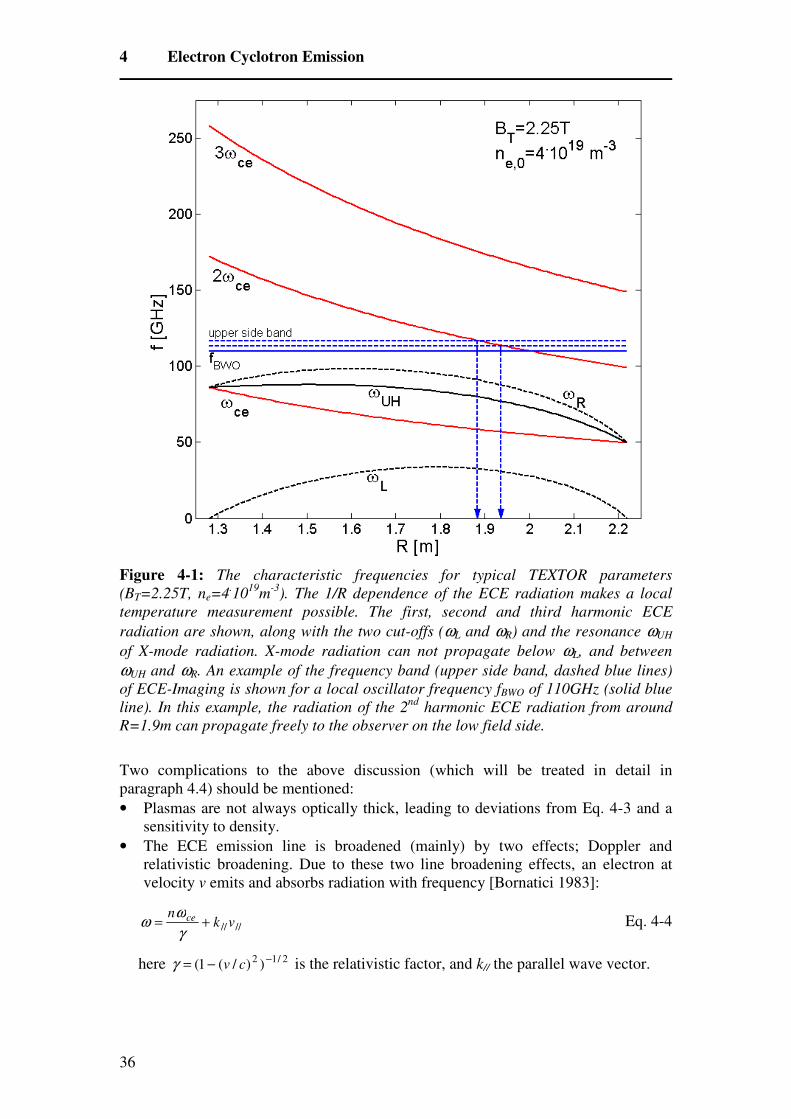
4 Electron Cyclotron Emission
36
Figure 4-1: The characteristic frequencies for typical TEXTOR parameters
(BT=2.25T, ne=4.10
19m
-3). The 1/R dependence of the ECE radiation makes a local
temperature measurement possible. The first, second and third harmonic ECE
radiation are shown, along with the two cut-offs (ωL and ωR) and the resonance ωUH
of X-mode radiation. X-mode radiation can not propagate below ωL, and between
ωUH and ωR. An example of the frequency band (upper side band, dashed blue lines)
of ECE-Imaging is shown for a local oscillator frequency fBWO of 110GHz (solid blue
line). In this example, the radiation of the 2nd
harmonic ECE radiation from around
R=1.9m can propagate freely to the observer on the low field side.
Two complications to the above discussion (which will be treated in detail in
paragraph 4.4) should be mentioned:
• Plasmas are not always optically thick, leading to deviations from Eq. 4-3 and a
sensitivity to density.
• The ECE emission line is broadened (mainly) by two effects; Doppler and
relativistic broadening. Due to these two line broadening effects, an electron at
velocity v emits and absorbs radiation with frequency [Bornatici 1983]:
Eq. 4-4
here 2/12 ))/(1( −−= cvγ is the relativistic factor, and k// the parallel wave vector.
////vkn ce +=
γ
ωω

Imaging and Control of Magnetic Islands in Tokamaks
37
Apart from these two complications, for practical application of ECE radiation as a
temperature diagnostic, the waves have to be able to propagate freely from the
emitting layer to the observation point. The propagation of electromagnetic radiation
in a magnetized plasma is (in the ‘cold plasma approximation’) described by the
Appleton-Hartree equation, giving the real part of the refractive index N [Bornatici
1983][Hutchinson 1987]:
Eq. 4-5
with θωω
ωωθρ 2
222
42 cos4sin
−+≡
ce
p.
Here θ is the angle between the direction of wave propagation and the magnetic field,
and the plasma frequency ωp is given by:
Eq. 4-6
One has to distinguish between O-mode radiation, whose electric field is oriented
parallel to B (minus sign in Eq. 4-5), and X-mode radiation, whose electric field is
oriented perpendicular to B (plus sign). For O-mode radiation, the electrons are
induced to oscillate parallel to B, making them insensitive to B. For perpendicular
propagation 2/πθ = , Eq. 4-5 for the O-mode reduces to:
Eq. 4-7
Like in a plasma without magnetic field, O-mode radiation has only one cut-off
(where N goes to zero) at the plasma frequency ωp. At a cut-off surface in the plasma,
radiation is reflected. No propagation is possible at frequencies below ωp where N<0.
For X-mode radiation, the electrons are induced to oscillate perpendicular to B.
Hence, apart from the plasma frequency ωp, here also the cyclotron frequency ωce
plays a role in the dispersion relation. For perpendicular propagation 2/πθ = , Eq. 4-5
for the X-mode reduces to:
Eq. 4-8
X-mode radiation has two cut-offs ωL and ωR:
Eq. 4-9
)(sin)(2
)(21
2222
222
2/
ρθωωω
ωω
ω
ω
mcep
ppXON
−−
−
−=
e
ep
m
en
0
2
εω =
2
2, 1
−=⊥
ω
ω pON
222
222
2, 1
pce
ppXN
ωωω
ωω
ω
ω
−−
−
−=⊥
( )
( )
++−⋅=
++⋅=
2/122
2/122
42
1
42
1
pceceL
pceceR
ωωωω
ωωωω

4 Electron Cyclotron Emission
38
and one resonance (where N goes to infinity and radiation is either absorbed or
converted to a non-propagating electrostatic oscillation) at the (upper) hybrid
frequency ωUH.
Eq. 4-10
X-mode radiation does not propagate at frequencies between ωUH and ωR, and below
ωL. In Figure 4-1 the characteristic frequencies for perpendicular X-mode radiation
are shown for typical TEXTOR parameters.
For practical application of ECE radiation as a temperature diagnostic, the waves have
to be able to propagate freely from the emitting layer to the observation point
(normally at the low field side), and there should be only one harmonic in the plasma
emitting at that frequency. For 2nd
harmonic X-mode radiation in TEXTOR (used by
ECE-Imaging at frequencies between 85 and 130GHz), this means that one should
stay above ωR, and avoid measurements very close to the high field side edge, as then
the 2nd
and 3rd
harmonics of ωce overlap in frequency. In Figure 4-1 an example of the
situation with ECE-Imaging tuned to 110GHz is shown.
Note that for ω >ωp for O-mode, and ω >ωR for X-mode radiation, the index of
refraction has values in the range 0<N<1 (phase velocities larger than the velocity of
light), meaning the plasma bends the lines of sight slightly outward.
4.2 The principle of an ECE radiometer
Before describing the ECE-Imaging system, first the principle of a conventional ECE
radiometer is discussed. The electronics of ECE-Imaging are basically the same as
those of such a conventional radiometer. A simple (fictive) heterodyne radiometer is
described in order to introduce the basic concepts like downconversion and the
bandwidths BIF and BV, important for ECE-Imaging.
An ECE radiometer measures the intensity of the (microwave) radiation from the
plasma in a certain frequency band. The central frequency of this band determines the
location of the emitting layer in the plasma, and (to first order) the bandwidth
determines the radial extent of this layer. The output signal is a measure of the
intensity of the radiation in this frequency band, and is linear with Te. By measuring
the ECE intensity in a number of frequency bands (corresponding to different radii R),
the Te profile can be determined. Wave accessibility and optical thickness normally
limit the possibilities for practical application of ECE as a Te diagnostic to only the
first harmonic O-mode and second harmonic X-mode ECE radiation. For typical
tokamak magnetic fields, this radiation has a frequency in the order of 100GHz. At
such high frequencies, (electronic) signal processing is difficult. Therefore, the (radio
frequency, RF) radiation from the plasma is downconverted to a lower frequency
(intermediate frequency, IF) before further processing. A radiometer that uses such a
downconversion is called a ‘heterodyne’ radiometer [Hartfuss 1997].
In Figure 4-2 a schematic representation of a (one channel) heterodyne ECE
radiometer is shown (from [Hartfuss 1997]). The radiation from the plasma is
222pceUH ωωω +=

Imaging and Control of Magnetic Islands in Tokamaks
39
downconverted by mixing it with the radiation of a so called local oscillator (LO) with
frequency fLO. In the mixer (M), the sum and difference frequencies of the two sources
are generated. The subsequent electronics are only sensitive to the (much) lower
difference frequency. This process does not differentiate between a positive and a
negative frequency difference, so a certain frequency f in the downconverted signal,
corresponds to two frequencies fLO+f and fLO-f in the plasma (RF) signal. In Figure 4-2
(bottom right) the two side bands (upper and lower side bands) are shown, that result
after band pass filtering the downconverted signal with a filter at central frequency fIF
and bandwidth BIF. To guarantee a measurement of Te at only one radius, one of these
frequency bands generally has to be filtered out (by a side band filter SBF) before
mixing the plasma and LO signals. The bandwidth BIF of the remaining side band then
determines (to first order, see paragraph 4.4) the radial extent of the emitting layer in
the plasma. The detector (SV) is basically a rectifier, converting the high frequency IF
signal to a signal that is a measure for the power in the IF frequency band (the so
called video signal). Finally, the signal is low pass filtered with a (video) bandwidth
BV, determining the time resolution of the radiometer. The higher frequency
fluctuations in the detector signal are averaged out (resulting in a smaller noise level)
to adapt the signal to the sampling frequency of the data acquisition system.
The above radiometer only measures one frequency band. Normally, radiometers have
more channels, each detecting a different frequency band. This can be done by for
instance splitting the signal before the IF filter BIF, and filter the separate branches
with different IF filters. ECE-Imaging uses a second downconversion step, mixing the
IF signal with eight different LO signals, to select eight frequency bands, see the next
paragraph.
Figure 4-2: Schematic representation of an ECE radiometer (reproduced from
[Hartfuss 1997]). The input ECE signal is mixed (M) with the radiation of a local
oscillator (LO with frequency fLO), after (optionally) filtering out one of the two side
bands with a filter (SBF). Subsequent filtering of the downconverted signal with a
band pass filter with bandwidth BIF and central frequency fIF determines the width
and frequency of the frequency band to which the radiometer is sensitive. The output
of the detector (SV) is a measure for the power in this frequency band. Finally, the
signal is low pass filtered with a bandwidth BV, determining the time resolution of the
radiometer.

4 Electron Cyclotron Emission
40
4.3 ECE-Imaging
A conventional ECE radiometer generally consists of a horn antenna at the low field
side plasma edge, receiving the ECE radiation of a single horizontal line of sight.
Neglecting broadening effects, the different frequencies of this ECE radiation
originate from different major radii in the plasma, due to the 1/R dependence of the
toroidal magnetic field. So by separating the ECE radiation into different frequency
bands (of bandwidth BIF), the radiometer measures the local Te at different radial
locations along the line of sight.
The ECE-Imaging diagnostic at TEXTOR ([Park 2003],[Park 2004],[Wang 2004])
yields real time 2D measurements of the local Te. This 2D capability is achieved by
replacing the single antenna of a conventional radiometer by a vertically aligned array
of 16 antennae, each observing a different horizontal line of sight (about 1cm apart) in
the poloidal plane of the plasma. Each of the 16 antennae is subsequently treated as a
conventional 8 channel (heterodyne) radiometer, resulting in a 2D array of 8 (radially)
by 16 (vertically) sampling volumes in the poloidal plane, representing an area of
approximately 7 by 16 cm.
Figure 4-3 shows the schematic setup of an ECE-Imaging system. Contrary to a
conventional radiometer, the ECE-Imaging antenna array is located outside the
tokamak. The ECE radiation from the plasma is observed through a large aperture
vacuum window, and imaged onto the array by (refractive or reflective) optics. To
facilitate the further processing of the signals, the radio frequency (rf) ECE radiation
is downconverted by mixing it with the radiation of a local oscillator, resulting in a
signal at the (lower) difference frequency. The local oscillator illuminates the antenna
array from the back.
Figure 4-3: Schematic overview of a 2D ECE-Imaging system. An optical system
images the ECE radiation from the plasma onto a vertically aligned (1-D) array of
detectors. Each detector views a different horizontal line of sight in the poloidal plane
of the plasma. From the back, the detectors are illuminated by a local oscillator to
downconvert the signal. By treating each detector as a conventional ECE radiometer,
the signals of each horizontal line of sight are split into radially separated
observation volumes.
The TEXTOR ECE-Imaging system is shown in Figure 4-4. The system observes the
plasma through a 42cm high, 30cm wide vacuum window, which is shared with the
Thomson scattering system. The optical path of the ECE radiation is shown by the red

Imaging and Control of Magnetic Islands in Tokamaks
41
line. Two large cylindrical mirrors, one planar mirror and 4 lenses image the radiation
onto the array. To assure the system is always in focus, the position of the focal plane
in the plasma can be radially adjusted by translating the lens before the array
(indicated by *). Also, on top of this lens, a (quasi-optical) notch filter can be placed
to protect the array against 140GHz stray radiation coming from the gyrotron. As
local oscillator, a so called backward wave oscillator (BWO) with a tuneable
frequency fBWO is used. The optical path of the local oscillator radiation is shown in
blue. The system is designed to observe the second harmonic X-mode ECE radiation
in a 4 GHz wide frequency band (at central frequency fBWO+5 GHz), representing a
radial section of about 7 cm in the plasma (depending on the local magnetic field
gradient). By changing fBWO, the ECE-Imaging system is tuneable over a frequency
range of about 85 to 130 GHz. Changing fBWO shifts the observation volume radially.
Under normal TEXTOR operation (BT=2.25 T) this provides access to the centre and
the low field side of the plasma.
ECE-I
Array
BWOMirrors
Lenses
PLASMA
MIR
*
beamsplitter
vacuum window ECE-I
Array
BWOMirrors
Lenses
PLASMA
MIRECE-I
Array
BWOMirrors
Lenses
PLASMA
MIR
*
beamsplitter
vacuum window
Figure 4-4: Layout of the combined ECE-Imaging/MIR system on TEXTOR. The
optical system consists of two large cylindrical mirrors and a set of lenses. The
optical paths of ECE-Imaging (red) and MIR (probing beam light green, reflected
beam dark green) are separated using a beam splitter. The ECE-Imaging array is
illuminated from the back (blue line) by a tuneable backward wave oscillator (BWO),
which is used as local oscillator. By vertically translating the lens indicated by the
asterisk (*), the radial position of the ECE-Imaging focal plane in the plasma can be
adjusted.
The two large cylindrical mirrors are shared with a second diagnostic, the Microwave
Imaging Reflectometer (MIR) [Mazzucato 2001], mounted in the same frame. The
optical paths of ECE-Imaging (red) and MIR (light and dark green) are separated by a
beam splitter (which is normally removed if only ECE-Imaging is operated). Contrary
to ECE-Imaging, MIR is an active microwave diagnostic; a 89 GHz probing beam
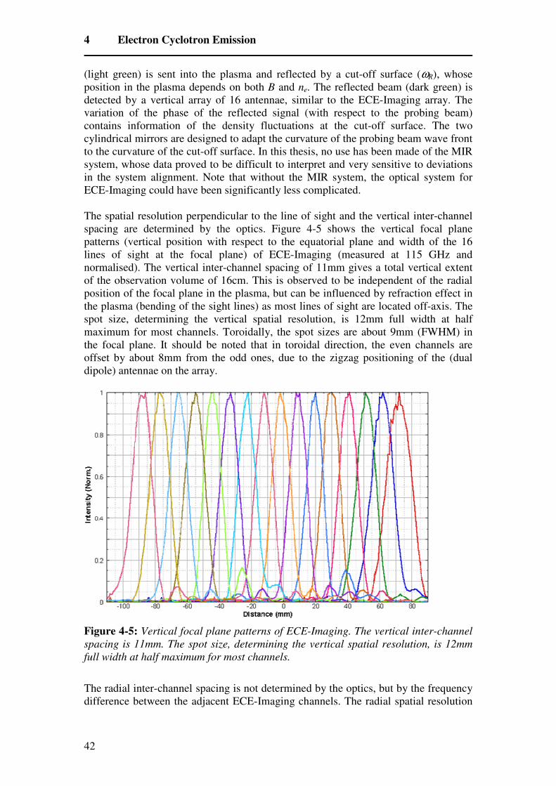
4 Electron Cyclotron Emission
42
(light green) is sent into the plasma and reflected by a cut-off surface (ωR), whose
position in the plasma depends on both B and ne. The reflected beam (dark green) is
detected by a vertical array of 16 antennae, similar to the ECE-Imaging array. The
variation of the phase of the reflected signal (with respect to the probing beam)
contains information of the density fluctuations at the cut-off surface. The two
cylindrical mirrors are designed to adapt the curvature of the probing beam wave front
to the curvature of the cut-off surface. In this thesis, no use has been made of the MIR
system, whose data proved to be difficult to interpret and very sensitive to deviations
in the system alignment. Note that without the MIR system, the optical system for
ECE-Imaging could have been significantly less complicated.
The spatial resolution perpendicular to the line of sight and the vertical inter-channel
spacing are determined by the optics. Figure 4-5 shows the vertical focal plane
patterns (vertical position with respect to the equatorial plane and width of the 16
lines of sight at the focal plane) of ECE-Imaging (measured at 115 GHz and
normalised). The vertical inter-channel spacing of 11mm gives a total vertical extent
of the observation volume of 16cm. This is observed to be independent of the radial
position of the focal plane in the plasma, but can be influenced by refraction effect in
the plasma (bending of the sight lines) as most lines of sight are located off-axis. The
spot size, determining the vertical spatial resolution, is 12mm full width at half
maximum for most channels. Toroidally, the spot sizes are about 9mm (FWHM) in
the focal plane. It should be noted that in toroidal direction, the even channels are
offset by about 8mm from the odd ones, due to the zigzag positioning of the (dual
dipole) antennae on the array.
Figure 4-5: Vertical focal plane patterns of ECE-Imaging. The vertical inter-channel
spacing is 11mm. The spot size, determining the vertical spatial resolution, is 12mm
full width at half maximum for most channels.
The radial inter-channel spacing is not determined by the optics, but by the frequency
difference between the adjacent ECE-Imaging channels. The radial spatial resolution

Imaging and Control of Magnetic Islands in Tokamaks
43
(spot size) is determined by both the bandwidth BIF of the ECE radiation selected per
channel, and broadening and absorption effects in the plasma described in the next
paragraph. The IF bandwidth BIF of 300 MHz, along with broadening effects in the
plasma, leads to a radial resolution of about 1 cm.
In Figure 4-6 a schematic layout of the ECE-Imaging electronics of a single antenna is
shown. The signal is downconverted two times. The first time at the array, by mixing
the plasma and BWO signals. This downconverted signal is transmitted out of the
TEXTOR bunker for further processing. After dividing the signal into 8 portions,
these are mixed with 8 local oscillator signals (at fLO=3.2, 3.8, 4.3, 4.8, 5.3, 5.8, 6.3,
and 6.8 GHz) in the second downconversion step. The frequency difference between
these local oscillators determines the radial inter-channel spacing of ECE-Imaging
and is hence 0.5GHz. This corresponds to typically 1cm in the plasma, depending on
the gradient of B. The resulting signals are band pass filtered (BPF, double sideband
5-150MHz), determining the bandwidth BIF (effectively 300MHz) of the ECE
radiation selected by each channel, which is important for the radial resolution of
ECE-Imaging. As only the amplitude of the signal is of interest (not the frequency of
the carrier wave), they are rectified by the detectors and low pass filtered (LPF). This
filtering (adjustable between 70Hz and 240kHz), determines the (video) bandwidth BV
and hence the time resolution of ECE-Imaging. The bandwidth BV corresponds to the
maximum detectable fluctuation frequency. The sampling frequency is normally set to
twice BV. Finally, the signals are converted to a digital signal by 12 bit ADCs, capable
of storing 2Msample per channel.
antenna
mixer
BWO
po
w
e
r
d
i
v
id
e
r
mixerBPF
detector
LPF
LO
antenna
mixer
BWO
po
w
e
r
d
i
v
id
e
r
mixerBPF
detector
LPF
antenna
mixer
BWO
po
w
e
r
d
i
v
id
e
r
mixerBPF
detector
LPF
LO
Figure 4-6: Schematic layout of the ECE-Imaging electronics of a single antenna.
The signal is downconverted two times. The first time at the array, by mixing the
plasma (antenna) and BWO signals. After dividing the signal into 8 portions, these
are mixed with 8 local oscillator signals (at 3.2, 3.8, 4.3, 4.8, 5.3, 5.8, 6.3, and 6.8
GHz) in the second downconversion step. The resulting signals are band pass filtered
(BPF), determining the bandwidth BIF (effectively 300MHz) and hence the radial
resolution of ECE-Imaging. After detection, the signals are low pass filtered (LPF),
determining the (video) bandwidth BV and hence the time resolution of ECE-Imaging.

4 Electron Cyclotron Emission
44
During the second downconversion step, in principle both the signal at frequency
fBWO+fLO (upper side-band) and fBWO-fLO (lower side-band) is selected. The radiation in
these two side-bands originates from different regions in the plasma. This would mean
that the ECE-Imaging signal would represent the average Te over these two (radially
separated) regions, which is of course unwanted. To avoid this, the lower side band is
blocked by a dichroic plate (a quasi-optical high pass filter) in front of the array, with
cut off frequency between fBWO-3.2GHz and fBWO+3.2GHz, so only the radiation in
the upper side-band with frequency fBWO+fLO is selected.
4.4 Radial resolution of an ECE diagnostic
The radial resolution of an ECE radiometer is determined by both the bandwidth BIF
of the detected ECE radiation, and by the radial width of the (not re-absorbed part of
the) emission profile. The emission profile j(R) (or j(ω)) is not a delta function as
suggested by Eq. 4-2, but is broadened by both relativistic and Doppler broadening.
The non-zero bandwidth BIF, (300 MHz for ECE-Imaging channels) results in an
emitting layer of width ∆R, determined by:
Eq. 4-11
For ECE-Imaging this is about 0.5cm. The width of the broadened emission profile
j(ω) due to Doppler ∆ωD and relativistic ∆ωrel broadening is given by [Bornatici
1983]:
Eq. 4-12
Eq. 4-13
where vth is the thermal velocity eeth mTv 2= (Te in J). Doppler broadening also
occurs for perpendicular observation θ=π/2, contrary to what is suggested by Eq.
4-12, as every radiometer has a finite sensitivity to parallel radiation. Alternatively
one can regard Doppler broadening for perpendicular observation as the natural line
width of the ECE radiation caused by the finite transit time of an emitting electron
through the observation volume. An alternative equation for ∆ωD, more relevant for
perpendicular observation, is given by [Sattler 1993]:
Eq. 4-14
where w0 is the waist of the Gaussian beam at the location of the resonance.
In Figure 4-7 the emission profiles j(ω) for both Doppler and relativistic broadening
are shown for Te=1keV and w0=12mm (which is the typical spot size of ECE-
Imaging). Expressions for the line shapes are taken from [Hutchinson 1987]. Due to
RRm
RneB
Rm
RneB
RRm
RneBB
eeeIF ∆−≈−
∆+=∆=
2
000000
)(ω
)cos(θωω Nc
vn th
ceD ≈∆
2
≈∆
c
vn th
cerel ωω
thD vw0
2ln22≈∆ω

Imaging and Control of Magnetic Islands in Tokamaks
45
the high spatial resolution of ECE-Imaging, the Doppler broadening is not negligible
compared to relativistic broadening (as for many other ECE radiometers with less
focused Gaussian beams). Analogously, instead of j(ω) at fixed R, one can regard j(R)
at fixed ω. For ECE-Imaging, Doppler and relativistic broadening result in radial
emission profiles with a full width at half maximum of about 1cm and 2cm
respectively. As in reality the two broadening effects occur simultaneous, a total
radial line width of about 3cm results.
Figure 4-7: Relativistic and Doppler broadening of the ECE radiation for Te = 1keV
as a function of (normalised) frequency. For the Doppler broadening, the ECE-
Imaging spot size w0=12mm is used. Relativistic broadening always shifts the
frequency down. Doppler broadening results in a symmetric profile with respect to
nfce. In reality, both effects occur simultaneous.
To determine the radial resolution of an ECE radiometer, another effect has to be
taken into account; the re-absorption of the emitted radiation. The radial resolution of
an ECE radiometer (neglecting BIF) is not determined by the width of the emission
profile j(R), but by the much narrower profile of radiation that actually reaches the
observer. The radiation emitted at the far side of the emission profile is largely
absorbed before it reaches the observer (generally at the low field side). The radiation
transport is governed by the following differential equation [Bekefi 1966]:
Eq. 4-15
)()()()(
2
2 ωωαωω
IjN
I
ds
dN −=
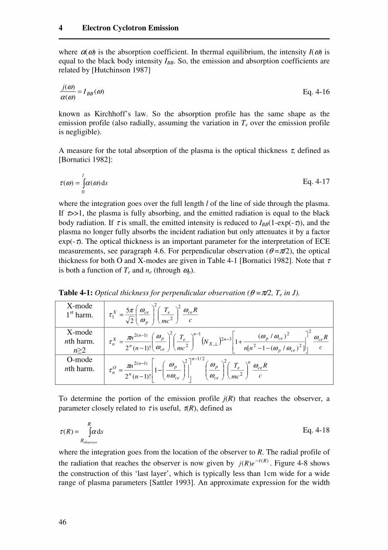
4 Electron Cyclotron Emission
46
where α(ω) is the absorption coefficient. In thermal equilibrium, the intensity I(ω) is
equal to the black body intensity IBB. So, the emission and absorption coefficients are
related by [Hutchinson 1987]
Eq. 4-16
known as Kirchhoff’s law. So the absorption profile has the same shape as the
emission profile (also radially, assuming the variation in Te over the emission profile
is negligible).
A measure for the total absorption of the plasma is the optical thickness τ, defined as
[Bornatici 1982]:
Eq. 4-17
where the integration goes over the full length l of the line of side through the plasma.
If τ>>1, the plasma is fully absorbing, and the emitted radiation is equal to the black
body radiation. If τ is small, the emitted intensity is reduced to IBB(1-exp(-τ)), and the
plasma no longer fully absorbs the incident radiation but only attenuates it by a factor
exp(-τ). The optical thickness is an important parameter for the interpretation of ECE
measurements, see paragraph 4.6. For perpendicular observation (θ =π/2), the optical
thickness for both O and X-modes are given in Table 4-1 [Bornatici 1982]. Note that τ
is both a function of Te and ne (through ωp).
Table 4-1: Optical thickness for perpendicular observation (θ =π/2, Te in J).
X-mode
1st harm.
c
R
mc
T cee
p
ceX ω
ω
ωπτ
2
2
2
12
5
=
X-mode
nth harm.
n≥2
( )c
R
nnN
mc
T
n
n ce
cep
cepnX
n
e
ce
p
n
nXn
ω
ωω
ωω
ω
ωπτ
2
22
232
,
1
2
2)1(2
])/(1[
)/(1
)!1(2
−−+
−= −
⊥
−−
O-mode
nth harm. c
R
mc
T
nn
n ce
n
e
ce
p
n
ce
p
n
nOn
ω
ω
ω
ω
ωπτ
−
−=
−−
2
22/1
2)1(2
1)!1(2
To determine the portion of the emission profile j(R) that reaches the observer, a
parameter closely related to τ is useful, τ(R), defined as
Eq. 4-18
where the integration goes from the location of the observer to R. The radial profile of
the radiation that reaches the observer is now given by )()( ReRj
τ− . Figure 4-8 shows
the construction of this ‘last layer’, which is typically less than 1cm wide for a wide
range of plasma parameters [Sattler 1993]. An approximate expression for the width
)()(
)(ω
ωα
ωBBI
j=
∫=l
s
0
d)()( ωαωτ
∫=R
Robserver
sR d)( ατ

Imaging and Control of Magnetic Islands in Tokamaks
47
∆Rlast of the last layer, valid for 2nd
harmonic X-mode radiation and τ2X>3 is given by
[Clark 1983]:
Eq. 4-19
The overall radial resolution of an ECE radiometer is now given by the convolution of
the broadened profiles due to the finite BIF (width ∆R) and the last layer (width ∆Rlast).
For ECE-Imaging, both normally have a width of the order of 0.5cm, resulting in a
typical radial resolution better than 1cm. Note that at low τ, the radial resolution will
get worse, as the last layer becomes broader.
Figure 4-8: Construction of the ‘last layer’. The radial resolution of an ECE
diagnostic is not determined by the width of the total emission profile j(R) (dashed
black line, here only showing the relativistic broadening), but by the part of j(R) that
actually reaches the observer. The part of j(R) furthest away from the observer is
largely reabsorbed, by a factor 1-exp[-τ(R)]. The dashed gray line gives (the
normalised) τ(R), the solid grey line e-τ(R)
. For a wide range of plasma parameters
(here Te = 1keV, τ2X=10 at 2fce=110GHz), the width of the last layer j(R)e
-τ(R) is less
than 1cm (solid black line).
7/62
7/42
7/22
2
22
)(
57.0
)(
804.0
)(
814.1)(
)(
XXX
X
e
eXlast
F
Rcm
TFR
ττττ
τ
++=
=∆

4 Electron Cyclotron Emission
48
4.5 Thermal noise
The signal of an ECE radiometer always fluctuates, due to the statistical nature of the
emission process. The ECE radiation consists of a large number of incoherent waves,
emitted by a plasma in thermal equilibrium. The beating of these waves results in the
so called ‘thermal’ noise, which is unavoidable and an intrinsic property of ECE
radiation. Normally, this noise dominates over all other noise sources caused by
(imperfections of) the diagnostic. The thermal noise level is primarily determined by
the bandwidths BV and BIF of the ECE radiometer [Bekefi 1966],[Hartfuss 1997]:
Eq. 4-20
Remember that BV determines the time resolution of an ECE radiometer and that the
radial resolution is (primarily) determined by BIF. So there is a trade-off between
spatiotemporal resolution and noise level. Increasing BV (better time resolution) or
decreasing BIF (better spatial resolution) increases the relative thermal noise level.
Figure 4-9: The experimentally observed thermal noise level of ECE-Imaging. The
relative noise level [(T-Tav)/Tav shown in the upper left graph] is independent of the
signal level, as seen here during the first 0.3s of TEXTOR discharge 98766 (a ‘norm-
shot’, using ECE-Imaging channel 3-1). Only at very low signal level (first 0.05s), the
relative noise level is enhanced due to a small base noise level of the ECE-Imaging
electronics (grey shaded area).During this first 0.3s no mode activity was detected, so
the fluctuations are predominantly due to the thermal noise. The relative fluctuations
(for 0.1s<t<0.3s) have the expected Gaussian distribution around the central Te (red
line), as shown by the lower right histogram. The root-mean-square value of the
relative fluctuations is 1.8%. This is somewhat less than the expected value of 2.5%
from Eq. 4-20.
IF
V
R
R
B
B
T
dT 22
=

Imaging and Control of Magnetic Islands in Tokamaks
49
Note that the thermal noise is a purely classical effect and is not caused by shot noise
due to the limited number of photons. Shot noise would result in a relative noise level
that becomes smaller at higher ECE intensities. Thermal noise, however, results in a
noise level that is independent of the signal level. This is also clearly seen in the
experimental ECE-Imaging data, of which Figure 4-9 gives an example. No (clear)
mode activity was observable in this time trace, so the fluctuations around the moving
average Tav (red line) can be assumed to be due to the thermal noise. The relative
noise level [(T-Tav)/Tav shown in the upper left graph] is independent of the signal
level, except for very low signal levels where the relative noise level is enhanced due
to a small base noise level of the ECE-Imaging electronics (grey shaded area). The
relative fluctuations (for 0.1s<t<0.3s) have the expected Gaussian distribution around
the central Tav, as shown by the lower right histogram. The experimentally observed
noise level of 1.8% is somewhat smaller than the prediction of 2.5% of Eq. 4-20
taking BIF=300 MHz and BV=100 kHz. The discrepancy could be caused by the non-
ideal video filter BV, which is only a first order filter and deviates significantly from
the sharp filter assumed in the derivation of Eq. 4-20.
4.6 Radiation temperature versus electron temperature
Ideally, the measured ECE intensity is a direct measure for the local Te. In reality, a
number of effects can lead to deviations between the measured radiation temperature
TR and the electron temperature Te. The effects of a non-fully absorbing plasma (so
small τ) are described, important for the interpretation of the experimental results
presented in chapters 5 and 6. Finally, some other possible sources of deviations are
shortly mentioned.
Only in optically thick plasmas (τ>>1) does the measured radiation intensity reach the
Rayleigh-Jeans intensity, and is consequently only a function of electron temperature.
In optically thin plasmas the measured radiation temperature TR can be expressed as
[Bornatici 1983]:
Eq. 4-21
where RW is the wall reflection coefficient. Radiation reflected from the back wall of
the tokamak passes through the resonant layer again and contributes to the radiation
intensity I. Note that this reflected wall component consists of radiation originating
from the full vertical extent of the radiating layer, and hence represents a vertically
averaged Te [Bornatici 1983]. On TEXTOR, the wall reflectivity RW is measured to be
about 0.7 [Udintsev 2003], although it should be noted that the (stainless steel) inner
tokamak wall has been covered by carbon tiles in the mean time, probably having a
smaller RW.
If one is only interested in the average value of Te, a plasma can be called optically
thick if τ>2. For fluctuations of Te, a higher value of τ is desirable. Since the optical
thickness τ is a function of both ne and Te, not only temperature fluctuations dTe, but
also density fluctuations dne will result in fluctuations of TR. Neglecting wall
τ
τ
−
−
−
−=
eR
eTT
W
eR1
1

4 Electron Cyclotron Emission
50
reflections for simplicity (RW=0) and assuming )1)(( τ−−+= edTTT eeR and
eee Tdnn )(~ +τ , the contributions from dTe and dne to the measured fluctuations dTR
can be estimated. A first order approximation gives [Sattler 1993]:
Eq. 4-22
here <> denotes an average and the factor a is always positive. For example, for τ=2
a=0.31 so about 30% of the density fluctuation level is seen in TR. For τ>6 density
fluctuations hardly influence TR. If the density and temperature fluctuations are in
phase, the fluctuation amplitude inferred from TR is an overestimation of the electron
temperature fluctuation amplitude. So for fluctuations, a more stringent lower limit
τ>6 should be utilised to regard a plasma as being optically thick.
Apart from optical thickness effects, deviations of TR from Te can be caused by e.g.:
• Finite sampling volume size: TR is an average of Te over the sampling volume.
Also, fluctuations with a wavelength comparable to or smaller than the sampling
volume size will be attenuated.
• Velocity distribution effects: An ECE radiometer is sensitive only to a selection
of the full (ideally Maxwellian) electron velocity distribution, because part of the
radiation is absorbed before reaching the observer. Deviations from a Maxwellian
velocity distribution (for instance due to the presence of a suprathermal electron
population) then lead to deviations between TR and Te. The radiation of a
population of fast electron can also be downshifted in frequency so much that it
overlaps with the next lower harmonic.
• Line bending: Outward bending of the observation line occurs due to the
variation in refractive index (0<N<1, see paragraph 4.1) Changes in the density
profile can lead to vertical oscillations in the position of the observation volume,
leading to fluctuations in TR (see for instance [Clark 1983]).
• Magnetic field fluctuations: Fluctuations in B lead to a radially fluctuating
position of the sampling volume, resulting in TR fluctuations (see for instance
[Sattler 1993]). This effect is normally negligible.
)exp(1
)exp()1(
τ
ττ
−−
−⋅=++= awith
n
dna
T
dTa
T
dT
e
e
e
e
R
R
Imaging and Control of Magnetic Islands in Tokamaks
51
5 2D edge temperature profile during DED 12/4 operation
5.1 Introduction
In chapters 8 and 9, the Dynamic Ergodic Divertor (DED) will be used as a tool to
generate and influence magnetic islands. The DED was however mainly built as a tool
to influence the magnetic field at the plasma edge in order to control the flow of heat
and particles towards the wall. The application of the DED perturbation field results
in the creation of the so called ergodic and laminar regions in the vacuum magnetic
field at the plasma edge. In the ergodic region, the magnetic field lines display chaotic
behaviour, no longer staying on a flux surface, but filling up a volume. The laminar
zone is located directly at the edge, where the perturbed field lines intersect the wall.
Here, the field lines have a short wall-to-wall connection length and don’t stay in the
plasma long enough to display the chaotic behaviour as in the ergodic region. In the
laminar zone a very complex structure of interwoven flux tubes with different wall-to-
wall connection lengths exits.
In this chapter, 2D ECE-Imaging measurements of the edge electron temperature
during DED 12/4 operation are presented. In the 12/4 DED coil configuration, each of
the 16 DED coils at the high field side carry currents that are 90 degrees phase shifted
with respect to the neighbouring coils. This current configuration results in a
perturbation field with a base m=12, n=4 mode structure. Due to the limited poloidal
extent of the DED coils, the perturbation field has strong side bands at other m values
close to 12. Because perturbation fields (in vacuum) decay as mcoilrr )/( for r<rcoil, the
12/4 perturbation field is only noticeable near the plasma edge (in contrast to the low
m perturbation field in the DED 3/1 configuration used in chapters 8 and 9). Both DC
and AC DED currents are possible.
The 2D capability of ECE-Imaging is used to investigate the edge temperature profile
during DED operation. The questions to be answered in this chapter are:
• Do we see an effect of the DED on the edge temperature profile? More specific,
do we see a 2D structure as expected from calculations of the edge magnetic field?
If yes, do experiment and theory show the same structures?
• How has the edge transport changed due to the DED, so how have the temperature
gradients changed?
• How controllable is the edge temperature profile? Do we see the expected strong
influence of the value of q at the edge (qa)?
If the last question can be positively answered, this would confirm the value of the
DED as a versatile tool to control and investigate the plasma surface interaction. To
answer these questions, two types of plasma discharges are used. For the investigation

5 2D edge temperature profile during DED 12/4 operation
52
of the transport changes, the DED and non-DED phases were compared in plasmas
with otherwise constant plasma parameters. For the investigation of the 2D structure
of the edge (and its evolution), discharges with a ramped plasma current were used.
5.2 The vacuum field edge properties.
This paragraph reviews the literature on the properties of the plasma edge during DED
operation. Based on the calculations of the magnetic field structure using the Atlas
code [Jakubowski 2004], one can differentiate between three regions in the plasma:
the laminar, ergodic and regular regions.
Figure 5-1: Schematic representation of the DED coils and the main plasma regions.
In the 12/4 configuration, the 16 coils at the high field side carry currents with 90
degree phase increments with respect to the neighbouring coils. This coil
arrangement results in a perturbation field with a main m/n=12/4 component
(resonant with q=3). Because the coils only cover part of the poloidal circumference,
also strong components at different poloidal mode numbers m are generated (mainly
m= 9, 10, 11, 13 and 14). Deeper in the plasma, magnetic islands in the vacuum field
are created at the resonant q surfaces. If the islands on two neighbouring resonant
surfaces (for instance q=10/4 and 11/4) are big enough to overlap, the magnetic field
becomes chaotic. This region is called the ergodic zone. Closer to the edge in the
laminar region, the field lines intersect the wall (the divertor target plates). Inside the
plasma core, the perturbation field in the 12/4 configuration (decaying with rm) has
no noticeable influence anymore. (Adapted from [Jakubowski 2004]).
In Figure 5-1, a schematic representation of the DED coils and the main plasma
regions during DED 12/4 operation is shown. When the DED is switched on, the
vacuum magnetic field topology changes drastically. At the resonant surfaces
(q=10/4, 11/4…) island chains appear in the vacuum field. These islands grow with
increasing DED coil current [w scales with (IDED)1/2
]. When neighbouring island
chains start to overlap, the field lines start to behave chaotically, no longer staying on
one flux surface, but filling up a volume. This plasma region is referred to as the
ergodic region. The amount of overlap between two island chains can be quantified by

Imaging and Control of Magnetic Islands in Tokamaks
53
the Chirikov parameter [Chirikov 1979] which is simply defined as the average width
of the two island chains divided by the distance between the two island chains.
Ergodicity of the field lines arises when the Chirikov parameter is larger than about 1.
Closer to the edge, the near field of the DED coils is dominant, resulting in perturbed
field lines that intersect the wall (the divertor target plates). These open field lines
have short wall-to-wall connection lengths LC, defined as the length of a field line in
the plasma between the two points where it intersects the wall, normally given in units
of poloidal turns (which is q2πR0 m). A complicated interwoven structure of flux
tubes with different LC exists. This plasma region is referred to as the laminar zone.
Deeper inside the plasma, the effect of the DED is no longer noticeable. This region
will be referred to as the regular zone.
In terms of field line topology, the laminar and ergodic regions can be defined by the
ratio of the connection length LC to the Kolmogorov length LK. The latter is a
characteristic length for the divergence of neighbouring field lines. Starting with two
field lines a distance d apart, after moving one Kolmogorov length parallel along
these field lines, the distance has (on average) increased to e times d. In the laminar
zone LC << LK, inhibiting ergodic field line behaviour. In the ergodic region LC is of
the same order of, or longer than, LK, making the magnetic topology ergodic. LK can
be determined by field line tracing, see below, and is found to be typically 15m (at a
Chirikov parameter of 1) [Kobayashi 2004].
So called Poincaré and laminar plots are used to visualise the ergodic and laminar
regions. These plots are generated using a set of computational tools called the ‘Atlas
code’ [Abdullaev 2003],[Jakubowski 2004]. This code calculates the trajectories of
individual field lines in the perturbed magnetic field configuration. For this purpose,
the field line equation in Hamiltonian form is used. The trajectory of a field line is
determined by
Eq. 5-1
where ))(),(),(()( τφτθττ r=x , and τ is a distance along the field line. Following
[Abdullaev 2003], this equation can be reformulated in Hamiltonian form by
introducing a new coordinate system, such that ),,( φϑψxx = . Instead of the minor
radius, now the toroidal flux ψ is used. The intrinsic poloidal angle ϑ , is defined such
that the pitch angle of a field line is constant over the flux surface. The magnetic field
is given by:
Eq. 5-2
and the field line equation Eq. 5-1 can now be expressed as:
Eq. 5-3
where H is the Hamiltonian. The equilibrium magnetic field is described by a
Hamiltonian H0 that is only a function of ψ. The full Hamiltonian describing the
perturbed magnetic field can be expressed as:
B
Bx=
τd
d
H∇×∇+∇×∇= φϑψB
ϑφ
ψ
ψφ
ϑ
∂
∂−=
∂
∂=
H
d
dH
d
d,

5 2D edge temperature profile during DED 12/4 operation
54
Eq. 5-4
where H1 is the perturbed Hamiltonian describing the DED perturbation field. H1 is
periodic in both ϑ and φ, and ε is a small dimensionless parameter.
The magnetic field structure can be visualised in a Poincaré plot. Such a plot is
generated by selecting a poloidal cross section and a collection of (starting points of)
magnetic field lines. These field lines are followed on their numerous toroidal turns
around the torus, and every time a field line intersects the poloidal cross section, this
is marked by a point. Instead of calculating the entire field line trajectories by
integrating the field line equation Eq. 5-3, a more practical (so called symplectic)
mapping has been developed [Abdullaev 2003]. Figure 5-2 gives an example of such
a Poincaré plot. Poincaré plots are ideal to visualise the ergodic regions, showing the
island chains and ergodic field lines.
Figure 5-2: Example of a Poincaré plot, clearly showing the chains of magnetic
islands at the various resonant surfaces. In the regions of overlap (here in particular
around r=41cm) the field lines fill up a volume. In the laminar region not a lot of
points are visible, as they leave the plasma after a small number of poloidal turns.
The laminar zone is characterized by finger-like structures of relatively long
connection length (Adapted from [Jakubowski 2004]).
The laminar region is not clearly visible in a Poincaré plot, because the field lines in
this region leave the plasma after a small number of toroidal turns, and hence leave
only a few points on a Poincaré plot. To visualise the laminar region, so called
laminar plots are used. These laminar plots are derived directly from the Poincaré
),,()( 10 φϑψεψ HHH +=

Imaging and Control of Magnetic Islands in Tokamaks
55
plots. They show the wall-to-wall connection length LC (in units of poloidal turns) of
the traced field lines. The distribution of the regions with different connections
lengths in the poloidal cross section is represented by marking these regions with
different colours. Examples of such laminar plots can be seen in Figure 5-3(e-h).
The topology of the DED induced structures and the level of ergodisation are mainly
determined by the q-profile (positions of the resonant surfaces qa) and the plasma
pressure, expressed in βpol. With increasing βpol the Shafranov shift enlarges the
distance between resonant surfaces on the HFS near the DED coils. This leads to less
overlap between the DED induced island chains (smaller Chirikov parameter), and
hence less ergodisation. Also, βpol influences the pitch angle of the field lines.
The existence of an ergodic region where the field lines behave chaotically and fill up
a volume depends on the presence of overlapping island chains. In the vacuum
magnetic field, represented by Poincaré plots, indeed overlapping islands and chaotic
field lines can be seen. However, the magnetic field topology in the presence of a
(conducting) plasma can be, and probably is, significantly different from the vacuum
topology. This will also be seen in chapter 8, where only above a certain threshold in
DED current a m/n=2/1 magnetic island is seen to be destabilized. Before
destabilization, no island is present, despite the fact that the vacuum field has an
island. Even after destabilization, the island differs from the vacuum island; it is larger
and has a (small) phase shift. The reason for this discrepancy is the shielding current
at the rational surface, which tries to cancel the externally applied perturbation field.
This current totally shields the inside of the rational surface for the perturbed field.
Whether an island is destabilized or not, depends on the relative rotation between the
plasma and the perturbation field. If the difference in rotation becomes zero, the island
is destabilized and growth to a width determined by the stability parameter ∆’ (can be
both larger and smaller than the vacuum island width). So the conclusion is that in the
presence of a plasma, the vacuum field plots can not be expected to give a realistic
picture of the actual magnetic field structure. All components of the DED field that
have a corresponding (intact) resonant surface in the plasma will generate a shielding
current. As long as there is a difference in rotation, the chains of vacuum islands, as
seen in Poincaré plots will be suppressed. Ergodic regions in the plasma can occur,
but only when the actual magnetic field structure has overlapping island chains.
In the laminar zone the field is dominated by the near field of the DED coils, resulting
in field lines that intersect the wall. Here, no shielding currents are possible and the
actual magnetic field can be expected to be close to the vacuum field. So it can be
expected that the vacuum field calculations give a good impression of the laminar
region. It is in the laminar region, where the most pronounced effects of the perturbed
field on transport are expected.
5.3 Edge transport during DED operation
The transport of heat and particles in the perturbed region is a balance between
perpendicular (collisional or turbulent) transport and parallel transport
(convection/conduction along field lines). As the perturbed magnetic field lines have a
radial component, both parallel and perpendicular transport can cause a radial loss of

5 2D edge temperature profile during DED 12/4 operation
56
heat and particles. The very complex structure of the edge magnetic field makes it
difficult to (analytically) estimate the transport levels. The plasma edge during DED
has a complicated (fractal) magnetic structure with entwined field lines of short and
long connection length. In particular, long thin ergodic ‘fingers’ (see Figure 5-2),
surrounded by laminar regions, connect the ergodic region with the wall. Whether a
plasma region behaves ergodic, laminar or regular is determined by the ratios between
the three parallel length scales that play a role:
• The Collision length, ( )eeie nT2850≈≈ λλ , (Te in keV, ne in 10
19m
-3) [Wesson
1997], typically 10m (at Te=100eV and ne=1.10
19m
-3).
• The Connection length LC, known from laminar plots, about 30m per poloidal
turn.
• The Kolmogorov length LK, typically about 15m.
In the regular region, both LK and LC are negligible compared to λ, so the particles
collide before they notice that they are on an ergodic or open field line. For ergodicity
to have an effect on transport, LK should be of the same order or smaller than λ. The
divergence of the field lines then contributes to the radial transport, and competes
with the radial step-size in a collision (ρe or ρi).
For transport to be effected by open field lines (the laminar region), LC should be of
the same order or smaller than the collision length λe, so particles that (diffusively)
enter the laminar zone almost certainly flow to the wall, making the laminar zone an
effective heat sink. It should be noted that the field lines in a region of the laminar
zone with equal LC, form a flux tube in which all field lines hit the wall at about the
same location. Hence, after a single collision, a particle is probably still inside that
same flux tube. So a number of collisions are needed for the particle to ‘jump’ to a
flux tube with a different LC. This number depends on the width of the individual flux
tubes.
Numerical modelling using the 3D plasma edge transport code EMC3-EIRENE
[Kobayashi 2004], predicts that electron temperature and density follow the
connection length profile, so in the fingers a higher Te is expected. This model is a
Monte Carlo fluid simulation, and uses the vacuum magnetic field topology as input.
Also the heat deposition profile on the divertor target plates (footprint) is predicted to
follow the structure of these long connection length fingers. Experimentally, both a
raised temperature and density in the fingers and the footprints are observed ([Lehnen
2005], [Finken 2006]). Note that both effects are attributable to the laminar region,
where the calculations (based on the vacuum field) are expected to be valid.
5.4 Experimental results
To investigate whether, and how, the temperature profile at the plasma edge during
DED operation depends on qa, a ramp of the plasma current with otherwise constant
plasma parameters is used. In Figure 5-3(a-d), ECE-Imaging measurements at the low
field side plasma edge during a shot with DC DED (IDED=11.5 kA, BT=1.91 T) are
presented. The evolution of the main plasma parameters is shown in Figure 5-4.
During this shot the plasma current was ramped down from Ip=450 to 200 kA. As BT
was kept constant, this means that the value of q at the edge (qa) was ramped up. The

Imaging and Control of Magnetic Islands in Tokamaks
57
data in Figure 5-3 is normalised to the temperature at t=1.5s, before switching on the
DED, and hence reflects the relative change in temperature during DED and the
current ramp. To reduce the thermal noise, the data is filtered using singular value
decomposition (a discussion of this filtering method is postponed to paragraph 7.1).
The data in Figure 5-3 represents only part of the current ramp and is taken between
t=2.5 and 2.75s. Figure 5-4 shows that during this time period, the central ne and Te
are almost unaffected by the DED and the current ramp, so the relative changes in Te
shown in Figure 5-3 (up to 50%) are limited to the plasma edge.
Figure 5-3(e-h) gives the corresponding laminar plots, as calculated with the Atlas
code [Jakubowski 2004]. Although the transition between laminar and ergodic regions
is hard to define, it is safe to assume that the 1 poloidal turn field lines belong to the
laminar zone and the 4 (or more) poloidal turn field lines belong to the ergodic (or
regular) zones. As the 2 and 3 turn field lines constitute only a thin layer, the
boundary between laminar and ergodic zones can be estimated fairly accurately. The
black contour indicates the approximate position of the observation volume of ECE-
Imaging. Due to uncertainties in both plasma position and ECE-Imaging alignment,
deviations are possible.
After switching on the DED, the temperature drops over the entire observation
volume of ECE-Imaging (all normalised temperatures below 1), which is a clear sign
of an enhanced transport level. The relative Te drop is largest near the edge. Apart
from the overall drop in Te, the measurements in Figure 5-3 show a clear 2D structure,
despite the fact that ECE-Imaging measured at the low field side, opposite to the
position of the DED coils. The main observations regarding the 2D structures are:
• The bottom half of the ECE-Imaging observation volume shows a poloidally
symmetric Te profile, while the top half (closest to the edge) shows a pronounced
poloidal asymmetry.
• The poloidally asymmetric part shows a ‘bulge’ of higher Te at the left hand side,
separated from the poloidally symmetric region. The poloidal position of this
bulge stays about the same during the current (q) ramp.
• The radial position of the bulge depends on q. It migrates radially inward with
decreasing plasma current. Due to the changing q profile, the DED induced
structures are expected to evolve; the resonant q surfaces migrate inward during
the ramp.
• The bulge merges with the poloidally symmetric region at a plasma current of
about 365 kA (Figure 5-3d).
The Atlas calculations in Figure 5-3(e-h) show very similar structures. They also
show a structure (a long LC region in the upper left, where two ‘fingers’ cross) which
migrates inward. In Figure 5-3(h) this structure connects to the main ergodic region at
the same time as the bulge in the ECE-Imaging measurements merges with the
poloidally symmetric main plasma The laminar plots show a new structure arising just
to the right of the ECE-Imaging observation volume. Also in the ECE-Imaging data,
Te is now observed to be higher on the right hand side. So the bulges seen with ECE-
Imaging corresponds to the long LC regions at the position where two fingers cross,
which is also confirmed by measurements with the He beam diagnostic [Schmitz
2006],[Jakubowski 2006]. The poloidally symmetric region at r<35cm observed with
ECE-Imaging corresponds to the LC>=4 poloidal turn region, located at about the
same radius.

5 2D edge temperature profile during DED 12/4 operation
58
Figure 5-3: Comparison of ECE-Imaging temperature measurements (a-d) with the
laminar plots (e-h) during a plasma current ramp down (TEXTOR discharge #96419).
The ECE-Imaging data is normalized to the Te before the DED phase, and hence
shows the relative Te drop in the poloidal plane. The laminar plots (Atlas
calculations) show the wall-to-wall connection length (in terms of the number of
poloidal turns) for the various (strongly deformed) flux tubes in the poloidal cross
section. The ergodic region is represented by the red, more than four poloidal turn
field lines. The thick black contours indicate the (approximate) position of the ECE-
Imaging observation volume. As the current ramps down, the resonant q surfaces shift
inward (down). Both the ECE-Imaging measurements and the laminar plots show an
inward migrating (high Te / long connection length) structure, joining the poloidally
symmetric region at about Ip=365 kA.

Imaging and Control of Magnetic Islands in Tokamaks
59
Figure 5-4: Overview of TEXTOR discharge #96419. The plasma current is ramped
down from 450 to 200 kA (at constant BT=1.91T) to vary qa. The 12/4 DC DED is
switched on between 2 and 3.5 s at 11.5 kA. The ECE-Imaging data is normalized to
the (radiation) temperature at 1.5s. The data of Figure 5-3 is taken between 2.5 and
2.75s (dashed lines). In this time interval the central Te and ne are still close to the
values at the moment of ECE-Imaging normalization and show no clear effect of the
DED.
To investigate the change in transport in the edge, a comparison is made between the
DED phase and the non-DED phase in a plasma with otherwise constant plasma
parameters (Ip=350 kA, ne≈1.5⋅1019 m-3
, BT=1.9T). As, apart from the DED current,
these phases are identical, the observed changes can be directly attributed to the DED.
In Figure 5-5a (normalised) ECE-Imaging data from a shot with DC DED
(IDED=12kA) is shown. The data again clearly shows a relatively hot bulge, separated
from the main plasma by a colder region, similar to the structure in Figure 5-3. The
corresponding laminar plot is shown in Figure 5-5b. In Figure 5-5c, estimates of the
absolute temperature profiles at cross sections 1 and 2 indicated in Figure 5-5a are
shown, along with the poloidally averaged profile and the non-DED reference case.
ECE-Imaging is not absolutely calibrated and has to rely on cross calibration or
profile shape assumptions. The absolute temperature values presented in Figure 5-5c
are derived from measurements with a different, calibrated ECE system, and the edge
profile shape (in the non-DED reference case) is estimated from He beam
measurements [Schmitz 2006]. The profile is taken linear inside the last closed flux
surface (at approximately R=2.11m), and exponentially decaying with an e-folding
length of 4cm outside the last closed flux surface.

5 2D edge temperature profile during DED 12/4 operation
60
Figure 5-5: Te profile during DED compared with non-DED reference (TEXTOR
discharge #96454). In a) the relative Te profile, normalized to the pre-DED profile,
shows a pronounced ‘relatively hot-spot’ and a ‘relatively cold channel’ separating it
from the main plasma. The laminar plot in b) shows a spot of high Lc at the same
position as the hot-spot [note that the radial coverage in figure a) is about twice as
large as in b)]. Assuming an unperturbed Te profile shape as shown in c) by the red
line, an estimate of the ‘absolutely calibrated’ profiles during DED is obtained. The
black line represents the poloidally averaged profile, the green and blue lines are the
profiles through respectively cross sections 1 and 2 in a). The flattening of these
profiles indicates enhanced transport. In d) the ratio between the observed Te
gradients and the non-DED reference is plotted, showing an increase in gradient of
about a factor of 3 inside the ‘cold channel’.
The profiles clearly show the overall drop in temperature and the large poloidal
variation in profile shape during DED. The extent of the DED affected region is
clearest seen in Figure 5-5d, where the ratio between the temperature gradient in the
non-DED reference case and the temperature gradient during DED is plotted.
Assuming heat flux and density profiles stay the same (which is an oversimplification,
certainly for the two poloidal cross section profiles due to poloidal redistribution of
heat flux) this ratio is a measure for the enhancement of the heat transport during
DED [Kobayashi 2004]:
Eq. 5-5
⊥
− ≈∇
∇
χ
χ erg
DEDe
DEDnone
T
T
,
,

Imaging and Control of Magnetic Islands in Tokamaks
61
Where χ⊥ is the effective perpendicular diffusion coefficient in the unperturbed case
and χerg is the (poloidally averaged) effective heat diffusion coefficient in the
perturbed magnetic field (containing both perpendicular and parallel transport and
hence is not a true diffusion coefficient). In Figure 5-5d, the poloidally averaged Te
gradient is observed to reduce by about a factor of two in the laminar region, meaning
that here the heat transport doubled (assuming the relative ne change was small
compared to the relative change in Te gradient). The two local temperature profiles
indicate a significant transport enhancement in the plasma regions where from Atlas
calculations the laminar zone is expected, here the gradients reduced by up to a factor
of three. In the regions corresponding to the ergodic region in the laminar plots (so
both the poloidally symmetric main plasma and the hot bulge), no significant
enhancement of heat transport is found. These local gradient changes are, however,
more difficult to link to changes in heat transport, as it can be expected that the heat
flux also has a poloidal variation (largest where the smallest Te gradients are
observed).
Caution is needed in quantitatively interpreting the ECE-Imaging edge measurements
due to two difficulties. First due to the lack of an absolute calibration and second, due
to the low optical thickness near the edge (typically, τ=0.5), meaning that not only Te,
but also ne changes are reflected in the measurements. As ne is seen to change in a
similar way as Te [Schmitz 2006], the relative temperature drop during DED is
overestimated (by about 30%). Qualitatively, the presented results are, however, not
sensitive to these two difficulties.
5.5 Summary and discussion
During DED 12/4 operation, an overall drop in Te is observed near the plasma edge.
Using the 2D capability of ECE-Imaging, a large poloidal variation in the Te profile is
observed. Moreover, these structures in the 2D Te profile depended on the value of qa.
The most prominent structure, a hot ‘bulge’ with relatively high Te, was seen to
migrate inward until it merged with the main, poloidally symmetric plasma. A
comparison of the ECE-Imaging data with the theoretical vacuum magnetic field
structure (laminar plots) shows that the hot bulge corresponds to a region in the
laminar zone of relatively large connection length at the position where two ‘fingers’
cross. The moment at which the bulge merges with the main plasma corresponds to
the moment at which the large connection length region connects to the ergodic
region, which has equally large connection lengths. The region in which ECE-
Imaging measures strong poloidal variations of Te is limited to the (small connection
length) laminar region.
The observed (overall) drop in Te is a clear sign of an enhanced heat transport in the
plasma edge during DED 12/4 operation. The relative change in Te gradient can be
used to estimate the relative change in heat conductivity. The poloidally averaged Te
gradient is observed to reduce by about a factor of two in the laminar region, meaning
that here the heat transport doubled. Inside the hot bulge, and in the poloidally
symmetric region, the transport levels are close to the unperturbed values.
5 2D edge temperature profile during DED 12/4 operation
62
The resemblance between the ECE-Imaging data and the laminar plots is not perfect,
which could be caused by inaccuracies in the reconstruction of the plasma equilibrium
going into the calculation of the laminar plot. In particular, the exact value of qa, and
hence the radial position if the large LC region, depends on the size and position of the
plasma. More general, one can not expect the two to be identical: ECE-Imaging shows
a temperature while the laminar plots show a connection length. The connection
length is probably more related to the gradient in Te than to Te itself.
So, it is observed that the DED has a large influence on Te profile and heat transport at
the plasma edge. Moreover, the exact edge topology can be selected by changing the
positions of the resonant surfaces near the edge. This makes the DED a flexible tool to
investigate the plasma-wall interaction.

Imaging and Control of Magnetic Islands in Tokamaks
63
6 Fluctuation measurements with ECE-Imaging
The experimentally determined transport levels in tokamak plasmas are one to two
orders of magnitude higher than predicted by neoclassical transport theory. This
discrepancy is generally ascribed to electrostatic plasma turbulence. Fluctuations of
the plasma electron temperature Te, electron density ne and electric field E can result
in additional radial heat (qe) and particle (Γe) fluxes according to [Cima 1995]:
Eq. 6-1
So not only the fluctuation levels, but also the phase relations between the various
fluctuating quantities are important. A wide variety of candidate (electrostatic)
turbulent modes, like the ion (electron) temperature gradient ITG (ETG) and trapped
electron modes (TEM), have been discussed in the literature, see [Horton 1999] for a
review. Apart from electrostatic turbulence, also imperfections of the magnetic field
topology can give rise to enhanced transport
Experimentally, many observations of broadband fluctuations with frequencies
between 50 and 500 kHz, and wave numbers k=2π/λ between 1 and 15 cm-1
[Horton
1999] are reported, mainly as density fluctuations. Experiments on TEXT-U [Cima
1995] provided the first evidence of broadband Te fluctuations using correlation ECE.
Later, similar measurements were reported from other tokamaks. The reported Te
fluctuation spectra show a broad peak, typically around 100 kHz. The observed
amplitudes increase with radius, typically ranging from about 0.5% near the plasma
centre to up to 10% at the edge. The limited spatial resolution of ECE diagnostics
generally restricts the measurements to wave numbers smaller than about 2 cm-1
.
Assuming also on TEXTOR broadband fluctuations are responsible for the anomalous
transport, ECE-Imaging should be able to measure them using correlation techniques
to suppress the thermal noise. The 2D character of ECE-Imaging would enable both
the radial and poloidal wave numbers and correlation lengths to be determined. This
chapter explores the capabilities of ECE-Imaging as a fluctuation diagnostic. To
illustrate the analysis techniques, two examples of fluctuation measurements will be
discussed: The so-called quasi-coherent mode [Krämer-Flecken 2003] near the plasma
edge and the ‘Alfvén-like’ mode [Zimmermann 2005] deeper into the plasma core.
The question whether or not broadband turbulence is present in TEXTOR,
comparable to the observations in other tokamaks, is addressed.
ESeeee
ESe
eESe
TBETnq
BEn
Γ+=
=Γ
23
23 /
~~
/~~
θ
θ

6 Fluctuation measurements with ECE-Imaging
64
6.1 Noise reduction by correlation
The ability of ECE-Imaging to detect high frequency fluctuations depends on the
signal to noise ratio, the time resolution and (for small wavelength fluctuations) the
spatial resolution. The main source of noise is the thermal noise inherent to any ECE
measurement. The thermal noise level depends on both the spatial and temporal
resolutions of the ECE measurement. Repeating some points from chapter 4:
• The spatial resolution in the direction perpendicular to the line of sight is
determined by the optics and is typically 12 mm vertically and 9 mm toroidally
(FWHM) in the focal plane (that can be shifted to ensure that the observation
volume is always in focus). The spatial resolution in the radial direction is
determined by the bandwidth of the ECE radiation selected by each channel (BIF)
and by the optical depth (which is a function of the plasma parameters). The IF
bandwidth BIF of 300 MHz, along with broadening effects in the plasma, leads to a
radial resolution below 1 cm for optically thick plasmas.
• The time resolution is determined by the video bandwidth BV of the system. The
maximum BV, and hence the maximum detectable fluctuation frequency, can be
varied, and is normally set to 100 kHz. The sampling frequency is normally set to
twice the video bandwidth.
• The accuracy of the Te measurements is determined by the thermal noise level,
which forms a fundamental limitation of ECE measurements. Increasing BV (better
time resolution) or decreasing BIF (better spatial resolution) increases the relative
thermal noise level according to [Bekefi 1966]:
Eq. 6-2
Taking BIF=300 MHz and BV=100 kHz gives a thermal noise level of about 2.5%.
This value is close to the experimentally observed noise levels of ECE-Imaging,
see chapter 4.
For a (periodic) structure in the plasma to be visible by ECE-Imaging, of course its
wavelength has to be at least twice as large as the spatial resolution. Also, the
fluctuation amplitude has to be big enough not to be ‘swamped’ by the thermal noise.
In ‘raw’ ECE data, normally only the largest plasma oscillations (magnetic islands
and the sawtooth oscillation) are visible. To detect fluctuations with smaller
amplitudes, the thermal noise has to be suppressed. Correlation (or the closely related
coherence) offers an effective method to do this.
Mathematically, the cross-correlation is the expectation value of the product of two
random processes S1(t) and S2(t) (two ECE signals in our case), both being functions
of t (time in our case), with one process shifted in t with a certain (time)lag l.
Eq. 6-3
where <> denotes the expectation value. In practice, only having finite time segments
of length N of discreet signals S(n), one can estimate the cross-correlation by:
IF
V
R
R
B
B
T
dT 22
=
)()()( 212,1 ltStSlC −=

Imaging and Control of Magnetic Islands in Tokamaks
65
Eq. 6-4
C1,2(l) can be seen as the dot product between S1 and S2, shifted by a time lag l.
Alternatively, the cross-correlation function can be obtained by convolving the two
signals with one of them reversed in time.
Eq. 6-5
Normally, the signals are ‘mean removed’, so only the fluctuating parts SSS −=~
are
used in the cross-correlation. In this case one also speaks of the cross-covariance. If
S1=S2 one speaks of the auto-correlation function. The amplitude of the (correlated
part of the) fluctuations is found by taking the square root of the amplitude in C1,2.
Correlated broadband phenomena with bandwidth Bw cause decaying contributions
(with increasing time lag) to C1,2 that fall off with a decay time [Sattler 1993]
Eq. 6-6
A special case is the correlated (broadband) thermal noise in an auto-correlation,
resulting in a sharp peak at zero time lag.
Figure 6-1 gives examples of (auto-)correlation functions for some idealized synthetic
signals. In real ECE signals, normally a mixture of different fluctuation types is
present (like sawtooth oscillations and magnetic islands). Suppose the signal consists
of fluctuations A and B, then C1,2 can be written as:
Eq. 6-7
If the various fluctuation types are mutually uncorrelated, the last two cross terms
vanish and the resulting correlation function is the sum of the contributions from the
individual fluctuation types (for long enough data segments).
It should be noted that the correlation function represents the average behaviour over
the integration period. If a certain fluctuation is only present during part of this period,
the amplitude in the correlation function will be correspondingly smaller, leading to
an underestimation of the fluctuation amplitude. It is also difficult to differentiate
between a fluctuation with an irregular frequency (of certain bandwidth), or a highly
coherent (constant frequency) fluctuation whose frequency gradually changes over the
integration period. So caution is needed in interpreting correlation functions.
As the cross-correlation of uncorrelated fluctuations is zero (at least in the
mathematical definition Eq. 6-3), the thermal noise can be suppressed by cross-
correlating two signals with independent noise. For two signals consisting of
[ ])()(1
)( 212,1 tStSN
lC −∗=
wB
12ln2/1 ⋅=
πτ
)()()()(
)()()()()()()(
2121
2121212,1
ltAtBltBtA
ltBtBltAtAltStSlC
−+−
+−+−=−=
<−
≥+
=
∑−−
=
0)(
0)()(1
)(
1,2
1
021
2,1
llC
lnSlnSN
lC
lN
n

6 Fluctuation measurements with ECE-Imaging
66
correlated Te fluctuations and uncorrelated noise, NTS~~
+= , the cross-correlation can
be written as:
Eq. 6-8
The last three terms represent correlations of uncorrelated fluctuation, and are hence
zero, only leaving the wanted Te fluctuations. For finite data segments, however, the
second (noise) term is only approximately zero (for sub-noise Te fluctuations the last
two ‘cross’ terms are negligible compared to the second). Correlating (discrete)
signals of length N reduces the noise by a factor of N1/2
. Because fluctuations are
contained quadratically in C12, the minimal detectable fluctuation level scales with
N-1/4
and can be written as:
Eq. 6-9
For ECE-Imaging data at maximal sampling rate, taking 2s of data (106 data points),
this theoretically leads to a minimal detectable fluctuation level of about 0.1 %.
Figure 6-1: Examples of correlation functions for typical signals. a) Correlating two
equal frequency harmonic functions with a phase shift results in a cosine of the same
frequency with a phase shifted maximum. b) (Auto-)correlating an oscillation which is
asymmetric in time (like a sawtooth), results in time symmetric oscillation in the
correlation function. c) Signals with irregular frequency result in a correlation
function with decaying amplitude for larger time lags. d) Signals with a different time
evolution of the amplitude result in an asymmetric amplitude of the correlation
function. e) Broadband fluctuations (bandwidth >= frequency) result in a single
decaying peak, larger bandwidths (for instance ‘white noise’) giving narrower peaks.
)(~
)(~
)(~
)(~
)(~
)(~
)(~
)(~
)()()(
2121
2121212,1
ltTtNltNtT
ltNtNltTtTltStSlC
−+−
+−+−=−=
IF
V
R
R
B
BN
tT
tdT4/1
2
)(
)(−=

Imaging and Control of Magnetic Islands in Tokamaks
67
As an alternative to the cross-correlation itself, one can use the cross spectral density
D1,2, which can be determined by either taking the Fourier transform of C1,2, or by
taking the product of the Fourier transforms of the individual signals:
Eq. 6-10
D1,2 is a complex quantity, containing both phase (the so called cross phase) and
amplitude information. If one is only interested in the amplitude information,
normally the coherence H is used, which is a normalized version of the cross spectral
density, and takes values between 0 and 1:
Eq. 6-11
The coherence is a powerful tool in analyzing coherent fluctuations. Broadband
fluctuations, however, are more easily detected using the cross-correlation function.
6.2 The Quasi Coherent mode
As a first example of high frequency, small scale fluctuation measurements with ECE-
Imaging, observations of the so called quasi-coherent mode are described. On
TEXTOR, this mode is first observed with the TEXTOR O-mode reflectometer
([Krämer-Flecken 2003],[Krämer-Flecken 2004]), but it is also observed with similar
experimental setup in FTU and T10 ([Vershkov 2001],[Vershkov 1999]). These
density fluctuations have a typical frequency of 50-100 kHz, amplitudes of up to a
few percent (highest near the plasma edge) and high poloidal mode number (around
m=50). The physical origin of this fluctuation is not yet conclusively resolved,
although in [Krämer-Flecken 2004] the ion temperature gradient mode (thought
responsible for the anomalous transport) is mentioned as a possible candidate.
The quasi coherent mode is also observed with ECE-Imaging, tuned to measure close
to the low field side plasma edge. In TEXTOR discharge #95097 (BT=2.25T,
Ip=400kA, ne,l.a.=2.7.10
19 m
-3, PECRH=800kW) both ECE-Imaging and the
reflectometer simultaneously observed the mode. Figure 6-2 shows Fourier spectra of
the reflectometer data during this discharge (around t=3.6s). The quasi coherent mode
is visible as a broad peak (on top of a much broader background) around 80 kHz, with
a bandwidth of roughly 50 kHz. The fact that the bandwidth of this fluctuation is
almost as large as its frequency provided its name.
With cross-correlation, using a second of data, the quasi coherent mode is also visible
with ECE-Imaging. The cross-correlation function shown in Figure 6-3 of two
neighbouring channels around R=2.17m (about 8 cm from the plasma edge), shows a
clear 90 kHz oscillation around zero time lag (superimposed on the sawtooth
oscillation and a weak 5 kHz fluctuation at larger time lags). From the decay of the
fluctuation amplitude with increasing time lag, a bandwidth of around 50 kHz can be
derived (Eq. 6-6), in good agreement with the simultaneous reflectometer
measurements at the same radius (Figure 6-2). The amplitude of the quasi-coherent
fluctuation in Figure 6-3 is about 1.5%. The smallest fluctuation amplitudes still
detectable using cross-correlation (for channels at smaller radii) were about 0.2% (see
)()()()( 2,1212,1 CFNSFSFfD ⋅==
)()(
)()(
2,21,1
2
2,1
2,1fFfF
fFfH =

6 Fluctuation measurements with ECE-Imaging
68
also Figure 6-5), proving that the minimum fluctuation levels predicted by Eq. 6-9 are
really accessible.
Figure 6-2: Double sided Fourier amplitude spectra of the fluctuations measured by
two channels of the O-mode reflectometer for TEXTOR discharge #95097. Apart from
the low frequency peak (<10kHz), a broad peak around 80kHz dominates the
spectrum. As the bandwidth of this peak (about 50kHz) is comparable to its frequency,
these fluctuations are called ‘quasi-coherent’. The slight asymmetry in the spectra is
probably caused by a combination of toroidal plasma rotation and small
misalignments of the (probing or receiving) antennae [Krämer-Flecken 2004].
The contour plots in Figure 6-4 show the cross-correlation function as a function of
channel separation ∆s (relative to a reference channel, channel 11-2, 3 cm below the
equatorial plane). In the cross-correlation function of poloidally separated channels a
phase shift is observed, increasing linearly with ∆s. From this phase shift as a function
of ∆s, a poloidal phase velocity of about 6 km/s can be deduced. From the ∆s needed
to get a phase shift of 2π the poloidal wavelength can be estimated to be around 7 cm
(or alternatively: λpol=vpol/f), from which a poloidal mode number around m=40 is
found. Since the analogous contour plot for radial separations does not show any
phase shift, it can be concluded that the radial velocity is zero (or too large to resolve,
as the phase shift is largest for slow propagating fluctuations).
The observed structures are periodic in poloidal, but not in radial direction. The
correlation drops quickly with increasing radial channel separation, giving a radial
correlation length in the order of 2cm. Part of this is however due to the drop in
fluctuation amplitude with decreasing radius. A poloidal correlation length is less
obvious to determine, due to the rotation in that direction. For a channel separation of
(-)7cm, so one wavelength, in Figure 6-4 almost no correlation is observed at zero

Imaging and Control of Magnetic Islands in Tokamaks
69
time lag, so the poloidal correlation length is at least smaller than 7cm. Note that at
the same channel separation the phase shifted maximum at a time lag of about 1.10
-5s
is still clearly visible. This means that the life-time of the rotating fluctuations (the
decorrelation time) is at least longer than 1.10
-5s.
Figure 6-3: Cross-correlation function of two [normalized and mean-removed
SSS )( − ] ECE-Imaging channels (channels 11_1 and 11_2) for the same TEXTOR
discharge as in Figure 6-2 (#95097). This correlation function represents a second of
data (t=3-4s). The low frequencies are dominated by the sawtooth oscillations.
‘Zooming in’ around zero time lag, first a weak, coherent (so also visible at larger
time lags) oscillation of about 5 kHz is visible. Zooming in further to even smaller
time lags reveals the high frequency (about 90 kHz), ‘quasi-coherent’ oscillation.
Quasi-coherent here means that the decay time of the oscillation is only slightly
longer than its oscillation period, so only a few oscillations can be discerned in the
correlation function. The relative fluctuation amplitudes (square root of the
amplitudes in the correlation function) are about 5% for the sawtooth and 1.5% for
both the 5kHz and the quasi-coherent oscillations.

6 Fluctuation measurements with ECE-Imaging
70
Figure 6-4: Contour plots of the correlation function of two spatially separated ECE-
Imaging channels, as a function of (poloidal or radial) separation. For both plots a
fixed reference channel (channel 11_2) is chosen. The left plot shows the correlation
function of this reference channel with poloidally separated channels. An increasing
phase shift with increasing channel separation is observed. From this phase shift a
poloidal rotation velocity of about 6km/s can be deduced. Furthermore, a poloidal
wavelength of about 7 cm (corresponding to a poloidal mode number close to m=40)
can be found from the figure as the poloidal separation between two maxima at
constant time lag. The right plot shows the correlation function of the reference
channel with radially separated channels. No phase shift is visible, meaning either
that the fluctuations do not propagate radially or that the propagation velocity is too
high to resolve.
The measured radial dependence of the fluctuation amplitude is given in Figure 6-5
(red curve). Because near the plasma edge a low optical thickness can be expected,
this amplitude cannot be directly interpreted as the temperature fluctuation amplitude.
For 2nd
harmonic X-mode radiation well below the cut-off frequency the optical
thickness τ02X
is [Bornatici 1983]:
Eq. 6-12
In optically thin plasmas (neglecting the possible influences of suprathermal radiation
and wall reflections) the measured radiation temperature TR can be expressed as:
Eq. 6-13
Since the optical thickness τ is a function of both ne and Te, not only Te fluctuations,
but also ne fluctuations will result in fluctuations of TR. Assuming dTe and dne have
the same phase, a first order approximation gives [Sattler 1994]:
( )τ−−= eTT eR 1
00
2
30
20
RB
RTn
cm
ekee
e
BX ⋅⋅=ε
πτ

Imaging and Control of Magnetic Islands in Tokamaks
71
Eq. 6-14
From the Te and ne profiles, the optical thickness τ and the parameter a of Eq. 6-14
can be calculated. The optical thickness is found to be about 1.5 at the outboard side
of the ECE-Imaging observation volume, rapidly increasing towards the plasma
centre. The general radial dependence of the density fluctuation amplitude (dashed
line in Figure 6-5) is known from reflectometer measurements [Krämer-Flecken
2003], so the ne fluctuation contribution to the measured TR fluctuations can be
estimated (a*dn/n) and is given by the blue line in Figure 6-5, which lies well below
the TR fluctuation amplitude. The shaded area indicates (1+a times) the estimated Te
fluctuation amplitude. So, despite all uncertainties, it is likely that the quasi coherent
mode is both a density and a temperature fluctuation. Figure 6-5 suggests comparable
amplitudes for both dTe/Te and dne/ne. Note that a possible phase difference between
dTe/Te and dne/ne results in a larger estimate for dTe/Te.
Figure 6-5: The radial dependence of the relative fluctuation amplitudes for the
quasi-coherent mode. The red line corresponds to the fluctuation amplitude of the
radiation temperature as measured with ECE-Imaging (derived from the auto-
correlation functions of discharge #95097) and can contain Te as well as ne
fluctuations. The dashed black line shows the average radial dependence of the
density fluctuation amplitude as it is measured by the O-mode reflectometer over a
large number of ohmic and neutral beam heated plasmas (always showing
approximately the same dependence) [Krämer-Flecken 2003]. The blue line is the
amount of parasitic density fluctuations in the ECE-Imaging signal expected from
dn/n and the optical thickness. As this curve lies well below the fluctuation amplitudes
measured by ECE-Imaging, this suggest a significant contribution of dTe/Te (the size
of the shaded gray area if there is no phase difference between the ne and Te
fluctuations).
)exp(1
)exp()1(
τ
ττ
−−
−⋅=++= awith
n
dna
T
dTa
T
dT
e
e
e
e
R
R

6 Fluctuation measurements with ECE-Imaging
72
6.3 Alfvén-like modes
An example of a high frequency fluctuation in the plasma core is the so called
‘Alfvén-like mode’. This fluctuation, normally associated with the simultaneous
presence of a magnetic island, was first reported by ([Zimmermann 2005],
[Zimmermann 2006]) on TEXTOR and [Buratti 2005] on FTU using magnetic pick-
up (Mirnov) coils. Again, there is little known about the physical origin of this mode.
As the frequency of this mode is observed to scale with the Alfvén velocity
eA nBv 0= (but well below the typical TAE frequency), it is called the Alfvén-like
mode. Figure 6-6 shows the spectrogram of a pick-up coil signal for a discharge
(#97215, BT=2.25T, Ip=270kA, PNBI=1.3MW) with two phases of Alfvén-like mode
activity. During the first phase, from about 0.55s to 0.7s, two bands of high frequency
fluctuations, at 25kHz and 43kHz, are visible. The second phase, from 2.3s onwards,
shows only the lower, 25kHz band which now shows a clear substructure. During
both phases, also a 2/1 tearing mode, with a frequency around 1kHz, was present.
Figure 6-6: Spectrogram of a magnetic pick-up coil showing two phases with ‘Alfvén-
like’ modes, one from 0.55 to 0.7s (with two bands at 25 and 43 kHz, highlighted by
blue circles) and another from 2.2 to 3.5s (with only the lower band, now clearly split
into two branches) [Zimmermann 2005]. With ECE-Imaging only the first phase is
visible.
A mode number analysis of the pick-up coil data [Zimmermann 2005], showed that
these Alfvén-like modes have low mode numbers (2/1 or 3/1) and that the two
strongest bands in the substructure (during the second phase) rotate in opposite
directions and differ in frequency by exactly twice the 2/1 tearing mode frequency.
The first phase doesn’t show a clear splitting of the bands, which might be due to the
lower frequency of the 2/1 tearing mode. Further, the central ne during the first phase
(1.5.10
19m
-3) is about twice as low as in the second phase (3.5
.10
19m
-3), whereas the
central Te is a bit higher (2keV in the first phase, 1.5keV in the second).

Imaging and Control of Magnetic Islands in Tokamaks
73
Figure 6-7: ECE-Imaging measurements showing a contour plot of the coherence as
a function of radius. The data of three identical discharges (#97211, #97213 and
#97215) is used to expand the radial range of ECE-Imaging to 15 cm as shown in a),
where the locations of the q=2 and 3 surfaces are estimated assuming a parabolic
current profile. In b), the coherence as a function of radius is shown, revealing that
the 25 and 43 kHz modes are spatially separated, most likely linked to the rational
surfaces. To improve statistics, for each radius the coherence (calculated over the
time interval 0.55-0.68s) of 15 neighboring pairs (1-2, 2-3, 3-4….15-16) of the 16
ECE-Imaging channels in poloidal direction is averaged.
With ECE-Imaging, only the fluctuations during the first phase are detectible. Figure
6-7 shows a contour plot of the coherence as a function of radius. For this plot, the
data of three identical discharges (#97211, #97213 and #97215), but with different
BWO frequency tuning of ECE-Imaging, was used to extend the radial range (see the
upper plot, also showing the estimated positions of the q=2 and 3 surfaces). For each
radius, the coherence is calculated using the data of neighboring channel pairs in
vertical (poloidal) direction. To improve statistics, the coherence functions of the 15
possible pairs for each radius (so pairs 1-2, 2-3,….., 15-16) are averaged. So, with an

6 Fluctuation measurements with ECE-Imaging
74
integration time of 0.13s (0.55 to 0.68s) and a sampling rate of 200kHz, effectively
4.10
5 data points are used for each coherence function.
Figure 6-7 shows that the two bands of Alfvén-like modes at 25 and 43kHz originate
from radially separated locations. The estimated locations of the q=2 and 3 resonant
surfaces (assuming a parabolic current profile) suggest that the 43kHz mode is
associated with q=2 and the 25kHz with q=3. The relative fluctuation amplitude is
about 0.3% for both bands (determined using cross-correlation), although the
coherence is somewhat higher for the low-frequency band (about 0.1).
During the second phase (>2.3s), the Alfvén-like modes where not visible with ECE-
Imaging. Possibly, because the amplitude is too small (suggested by the weaker pick-
up coil signal). Again, caution is needed in interpreting the fluctuations as Te
fluctuations. Due to the relatively low density during the first phase, the optical
thickness ranged from about 1 for the outermost channels to 6 for the innermost. So,
although for the innermost channels the parasitic ne fluctuations can safely be
neglected, for the outermost channels a (Eq. 6-14) is about 0.5.
6.4 Conclusions and discussion
The two examples of fluctuation measurements show that the detection of fluctuations
with amplitudes significantly (more than an order of magnitude) lower than the
thermal noise level is possible using cross-correlation techniques. The lowest detected
fluctuation amplitude of about 0.2% is close to the predicted sensitivity for correlation
techniques.
The most pronounced example of a high frequency fluctuation is the quasi coherent
mode at the plasma edge. The amplitude of this mode, about 3% at the very edge,
decreases rapidly with decreasing radius until it is no longer detectible by ECE-
Imaging. The ECE-Imaging measurements suggest ne and Te fluctuations are
comparable in amplitude for this mode. Radial and poloidal correlation length of a
few cm and a decorrelation time of about 1.10
-5s are observed. The measurements of
the quasi-coherent mode demonstrated that ECE-Imaging is (at least) sensitive to
fluctuations with f <= 100kHz, λ >=0.07m (k<=1cm-1
), and relative amplitude larger
than 0.2%
Deeper into the plasma core, the observation of high frequency Te fluctuations with
ECE-Imaging is rare. The Alfvén-like mode is an example of a high frequency, low
mode number fluctuation that is visible. The ECE-Imaging data shows that the
different branches of this fluctuation originate from different radii, and are probably
related to the rational q surfaces.
Can ECE-Imaging observe the broadband turbulence responsible for the anomalous
transport? In [Krämer-Flecken 2003/2004] it is argued that the quasi-coherent
fluctuation is the ITG mode. Indeed the ECE-Imaging data of this mode is very
reminiscent of the broadband turbulence measured by for instance [Cima 1995].
Frequency, bandwidth, wave number and the radial dependence of the amplitude are
all comparable. Only the absolute value of the amplitude is somewhat smaller (0.2%
in the centre instead of 0.5%), causing the fluctuations to drop below the statistical

Imaging and Control of Magnetic Islands in Tokamaks
75
noise level. It is however known from the O-mode reflectometer measurements that
the mode is also present deeper into the plasma core with density fluctuation levels of
about 0.3% at half radius [Krämer-Flecken 2003]. These measurements also show that
further inside the plasma, the wavelength of the mode decreases, the wave numbers
increasing from about 1 cm-1
at the edge up to about 3 cm-1
at ρ=0.4. For reference,
ECE-Imaging is designed to be sensitive for k<2.8 cm-1
[Park 2003]. So, both the
smaller wavelength and the smaller amplitude make the fluctuations harder to
measure with ECE-Imaging. In [Cima 1995] it was already demonstrated that the
fluctuation levels depend very critically on the focussing (transverse spatial
resolution) of the ECE channels, indicating a large part of the fluctuation amplitude is
attributable to higher k components. So it can be concluded that the broadband
fluctuations are at the edge of the capabilities of ECE-Imaging; visible at the edge, but
not in the centre.


Imaging and Control of Magnetic Islands in Tokamaks
77
7 Experimental determination of the island parameters
ECE-Imaging produces large amounts of data, which, in its raw form, is often hard to
interpret. For the analysis of magnetic islands, described in chapters 8 and 9,
parameters like island width and Te profile are needed, which cannot be directly
extracted from the raw ECE-imaging data. Data of the time history of one full island
rotation period is used to make a 2D poloidal reconstruction of the island. This way of
visualizing the ECE-imaging data greatly facilitates the interpretation and analysis of
(nearly) constant frequency magnetic islands. The procedure to extract the island
parameters is described in this chapter.
7.1 Calibration and filtering
Before constructing the poloidal reconstruction, the ECE-Imaging data is (cross)
calibrated on Thomson scattering and filtered using Singular Value Decomposition.
The ECE-Imaging system itself is not calibrated. The 128 channels all have different
sensitivities (Volts per keV) and offsets. For a meaningful 2D visualization of the
data, some kind of calibration is necessary. Often, a relative calibration (for instance
by normalizing the channels to their average value) is sufficient, which doesn’t
require another calibrated Te diagnostic. If, however, the absolute value of Te, or the
shape (mainly the radial gradient) of the Te profile are important, the ECE-Imaging
data has to be cross-calibrated with a different calibrated Te diagnostic. For the study
of magnetic islands, the ECE-Imaging system is cross-calibrated with the Thomson
scattering diagnostic. Thomson scattering measures the Te profile during one or more
(typically 10) short pulses along a vertical chord in the plasma slightly displaced from
the plasma centre, see chapter 3. By estimating the shape of the magnetic flux
surfaces in equilibrium (mainly the Shafranov shift), the Thomson Te profile can be
projected on the equatorial plane and directly applied to calibrate ECE-Imaging. The
ECE-Imaging channels are cross calibrated by setting the measured average Te during
(a small time window around) the Thomson pulses equal to the (projected) Thomson
Te at the corresponding minor radius. As m/n=2/1 islands are roughly located at half
radius, this procedure is not very sensitive to uncertainties in the position of the
plasma centre. Also, ne and Te are large enough for the plasma to be optically thick, so
the ECE-Imaging signal does not contain a parasitic ne contribution.
To reduce the thermal noise inherent to all ECE diagnostics, the 2D data is filtered
using Singular Value Decomposition (SVD), a standard mathematical technique to
decompose matrices into biorthogonal pairs of eigenvectors. SVD is a powerful tool
in analyzing data of diagnostics with a large number of spatial channels, all

7 Experimental determination of the island parameters
78
representing comparable data ([Nardone 1992],[Dudok 1994]). The ECE-Imaging
data of N time samples from the 128 channels builds an N by 128 matrix. SVD splits
this data into 128 pairs of orthogonal space and time eigenvectors of respectively
length 128 and N, the so called topos-chronos pairs, which are specific for the given
data set. The eigenvalues of these eigenvector pairs are called the ‘singular values’.
One can compare SVD to Fourier analysis. The Fourier components are the analogues
to the singular values. The difference is that Fourier analysis expands the data in the
orthogonal basis of harmonic functions, whilst SVD expands the data in the
orthogonal basis of eigenvector pairs specific for the data set under consideration.
This can be a large advantage: An infinite number of Fourier components is needed to
describe a sawtooth, while in SVD only one chronos is needed. Also, if data can be
represented by only one eigenvector pair, SVD does represent it by only one pair with
(large) nonzero eigenvalue. If, on the other hand, the data is totally incoherent
(uncorrelated white noise on all channels), SVD needs all 128 eigenvector pairs, all
with comparable (low) eigenvalue, to describe the data.
By only keeping the eigenvectors with the largest eigenvalues, the data is filtered. The
more redundancy (so double information) in the data, the less eigenvector pairs SVD
needs to accurately describe the data and the more accurate these eigenvectors are.
There is a large amount of redundancy in the ECE-Imaging data of islands. Because
the islands rotate poloidally, all information is seen 16 times by the 16 vertical
channels, only slightly phase-shifted. Also the data from the 8 radial channels display
large similarities. It can hence be expected that the (coherent part of) this data can be
described by a small number of eigenvector pairs. To avoid throwing away physics,
the number of SVD components kept, is taken larger than strictly necessary. Typically
the highest 30 of 128 eigenvector pairs are kept for describing magnetic island data.
So the SVD filtering throws away most noise (roughly three quarters), and keeps
practically all (coherent) physics, without limiting the space or time resolution of the
signals (as is the case in ‘smoothing’).
7.2 Poloidal reconstruction of the island
To visualize the ECE-Imaging data in an easily interpretable way, a poloidal
reconstruction is used. From this reconstruction of the ‘full’ 2/1 island, the main
island parameters like island width and Te profile are extracted. Figure 7-1 gives a
typical example of ECE-Imaging data of a 2/1 magnetic island. The observation
volume of ECE-Imaging is about 8 by 16 cm, for the island experiments located at the
q=2 surface at the low field side of TEXTOR, see Figure 7-1b. The minor radius of
the q=2 surface is typically 30 cm (the TEXTOR minor radius is 47 cm), so ECE-
Imaging covers less than 10 % of the poloidal circumference of the q=2 surface. It is
therefore hard to get a comprehensive view of the mode structure from the ‘raw’ data,
as at any time only a small part if the island is observed by ECE-Imaging. The plasma
around the q=2 surface is assumed to rotate like a rigid rotator (constant velocity as a
function of minor radius), which is confirmed by the phase velocity as a function of
radius measured by ECE-Imaging. It is therefore possible to map the data for one full
island rotation period onto a poloidal shell to visualize the entire poloidal mode
structure (see Figure 7-2). In this mapping, time takes over the role of the poloidal
angle. As every part of a rotating magnetic island is measured by more than one ECE-
Imaging channel, there is a large amount of redundancy in the data (the 16 vertical

Imaging and Control of Magnetic Islands in Tokamaks
79
channels of each column see the same part of the island, only time shifted). Using
only one radial row of 8 channels for the reconstruction already gives a good result,
because the (redundant) information of the other 15 rows is already used in the
Singular Value Decomposition to determine the spatiotemporal eigenvectors, and the
statistics for all 128 channels is hence contained in the SVD filtered signal for this one
row of 8 channels. So although the 2D character of ECE-Imaging is not directly used,
the analysis does profit from the large number of available channels. The rotational
reconstruction is a representation of the mode structure of the island as observed at the
low field side, assuming a constant rotation velocity around a perfectly circular
poloidal shell. In reality the rotation velocity can vary around this shell, as long as the
mode frequency stays constant (so a higher poloidal velocity has to be cancelled by a
larger poloidal wavelength). Also, the real island probably has a different shape at the
high field side (more symmetrical with respect to the q=2 surface). The
reconstruction, however, is mainly used to derive the width of the island (at the low
field side), which is insensitive to these effects and the exact shape (q=2 surface might
be slightly noncircular) and radius of the reconstructed shell. A reconstruction
contains data of a full poloidal rotation period (2 ms), and the derived island
parameters are hence an average over this period. So, the procedure is only valid if the
changes in the mode structure are slow compared to the rotation period.
Figure 7-1: a) Typical ECE-Imaging Te time traces of a 2/1 magnetic island
(#99183). At 2.2s a local heating source (ECRH) is introduced inside the island. b)
The position of the three channels with respect to the q=2 surface. For channels
inside the island radius, the maxima in the signal correspond to the time at which the
X-point passes by the observation volume. Channels outside the island radius show
maxima if the O-point passes by. So there is a phase inversion between the inner and
outer channels. Note the increasing O-point Te peaking in the central channel after
ECRH switch on.
Two typical examples of poloidal island reconstructions are shown in Figure 7-2.
Without a large heat source, the Te profile inside the island is (almost) flat, as in the
left reconstruction. The elliptically deformed plasma centre is clearly visible. If, as is

7 Experimental determination of the island parameters
80
shown in the right reconstruction, heat is deposited inside the island (here by ECRH),
the Te profile becomes peaked at the O-point, revealing the full island structure.
Figure 7-2: Typical examples of poloidal island reconstructions. The left plot shows
an island with a flat Te profile. The hotter plasma centre is approximately elliptically
deformed. At the right, a (ECRH) heated island with a peaked Te profile is shown. The
maximum of this peaking corresponds to the O-point.
7.3 The fitting procedure
An algorithm is used to extract the main island parameters from the poloidally
reconstructed ECE-Imaging data. This enables to analyze the large amount of data in
an objective way. To determine the island width, an ellipse (at temperature Tell) is
fitted to the data, see Figure 7-3. A standard least mean squares fit, minimizing the Te
deviation between the ellipse and the data, is used to fit the ellipse to the data, which
is regarded as a surface in the 3D (r,θ,T) space (in the 2D projection in Figure 7-3, the
Te direction is colour coded). The fitted ellipse has four free parameters: major radius
a, minor radius b, orientation angle θell and temperature Tell. The difference between
the major radius a, and minor radius b of this ellipse gives the displacement (radial
excursion) of the fitted Te contour, and is a measure for the width of the island. This
method works for islands with and without a peaked Te. Also, not the entire island has
to be visible (which is often the case due to the limited radial extent of the ECE-
Imaging channels). The four free parameters of the ellipse are too much to be fitted in
one step, so first a ‘trial’ ellipse with fixed [a,b] is fitted to find the [θell,Tell].
The minor radius a of the ellipse is chosen such that the ellipse is slightly smaller than
the inner separatrix of the island, to ensure it lies in the steep Te gradient of the hot
central plasma. If the fitted ellipse is chosen too large (too close to, or even larger than
the inner island separatrix), the flat Te gradient inside the (unheated) island separatrix
causes the fit to behave unstably (the deviation between ellipse and data becomes
independent of b). The wanted value of a-b is insensitive to the exact size of the
ellipse, as long it is close to the size of the inner separatrix. Also, a-b is only meant as

Imaging and Control of Magnetic Islands in Tokamaks
81
a measure for w, which is also true if the fitted ellipse is smaller than the island
separatrix.
For islands with a peaked Te profile (ECRH heated), the O-point position (rmax) and
temperature (Tmax) are found by looking for the Te maximum on the minor axis of the
fitted ellipse. Also, the exact position of (a point of) the inner separatrix can be
determined by finding the minimum Te between the O-point and the fitted ellipse.
Figure 7-3: Overview of the various parameters that are determined by the fitting
procedure, being the four free parameters [a,b,θ,T]ell of the ellipse, the radius and Te
of the O-point, the position of a point on the separatrix and the correction factor C
needed to overlay the ellipse with this point on the separatrix.
As mentioned, the fitted ellipse is too small to represent the (inner) separatrix. This
can be corrected for by introducing a correction factor C, defined such that Ca and Cb
are the major and minor radii of the ellipse passing through the found separatrix
position.
Two definitions of the full island width w can be used, see Eq. 7-1. First, the
difference between major and minor radii of the fitted ellipse is a measure for the
island width, with an unknown proportionality constant A. Second, twice the
difference in radius between O-point and (corrected) minor radius of the ellipse. The
second definition is a direct measure for the island width, but is only useable for
heated (peaked) islands. The second definition can be used to calibrate the first
method, yielding a typical proportionality constant A of 1.5 (the exact value has to be
determined from experiment to experiment).

7 Experimental determination of the island parameters
82
Eq. 7-1
The Te profile inside the island is evaluated on a circle through the O-point (see
Figure 7-4). In this way the (relative) Te profile is independent of any (relative)
calibration errors, since all points on a circle are measured by the same ECE-Imaging
channel(s). An example of a Te profile inside an island is shown in Figure 7-4 (the red
line). The Te is plotted versus the normalized effective island radius ρ*, related to the
island flux surface label Ω (see chapter 2) as
Eq. 7-2
Going once around the circle through the O-point, the Te profile is seen four times
(the four black lines in Figure 7-4) as the values of Ω repeat themselves. The Te
profile used in the analysis is the average of these four profiles (the red line). As the
islands are generally slightly asymmetric, the O and X-points lie on slightly different
minor radii, and part of the Te outside the island (Ω > 1) is visible on the circle
through the O-point. The separatrix corresponds to the minimum Te on the Te profile,
fixing ρ*=Ω = 1. The Te peaking ∆Te is defined as the difference between O-point and
separatrix Te.
In the next two chapters, the island parameters derived as described here play a central
role.
Figure 7-4: a) Circle on which the Te profile is evaluated. As all data points on the
circle are measured by the same ECE-Imaging channels, this Te profile is insensitive
to relative calibration errors. b) Example of a Te profile inside an island as a function
of the normalized island radius ρ*. Going once around the circle, the Te profile is
observed four times. The minimum in the average profile determines the position of
the separatrix. The part outside the separatrix (grey area) is discarded. The difference
between O-point and X-point Te is referred to as ∆Te.
)(2)( max CbrbaAw −≈−≈
2
1*
+Ω=ρ

Imaging and Control of Magnetic Islands in Tokamaks
83
8 Dynamics of tearing modes in the presence of a perturbation field
*
Abstract. The influence of a magnetic perturbation field on the dynamics of
tearing modes in the TEXTOR tokamak is investigated. A set of experiments
is performed to quantitatively test the generally accepted theory, mainly
developed by Fitzpatrick. The perturbation field is generated by the Dynamic
Ergodic Divertor (DED). This perturbation field causes shielding currents to
flow on the resonant q surfaces which have two effects: they alters the
stability of tearing modes and exert a torque on the rational surfaces,
influencing the plasma rotation. The rotation frequency and width of tearing
modes, as well as the relative phase shift to the perturbation field are
measured with the ECE-Imaging diagnostic. The evolution of the island
width (determined by a modified version of the Rutherford equation) and the
processes of mode penetration and unlocking (determined by the balance of
all torques acting on the island) are compared with theory using a numerical
simulation, giving satisfying agreement.
8.1 Introduction The formation of tearing modes (or magnetic islands) in tokamaks decreases the
global confinement of energy and particles, and hence should generally be avoided.
Furthermore, large islands can lead to plasma disruptions. Magnetic perturbation
fields resonant with the island are capable of both generating an island, and locking a
pre-existing island. Although perturbation fields normally work destabilizing, they
can also be used to suppress islands ([La Haye 2006], [Lazzaro 1988]). Perturbation
fields are present in all tokamaks. Two examples are the stationary error field caused
by deviations of the magnetic field from axisymmetry (for example due to coil
misalignments and the field ripple), and the perturbation field a rotating island causes
by inducing currents to flow in a conducting wall or on a different resonant surface.
So the interaction of tearing modes with perturbed magnetic fields is of major
importance for the understanding of tearing mode dynamics. Experimental
investigation of this interaction is normally difficult, because the perturbation field is
in general unknown and uncontrollable, enabling only a qualitative comparison with
theory ([Morris 1992b], [Savrukhin 2000]). This paper describes a set of experiments
on the TEXTOR tokamak, using the very controllable and fully known (rotating)
perturbation field of the Dynamic Ergodic Divertor (DED) [Special Issue 1997]. In
these experiments the DED perturbation field strength is increased until an m/n=2/1
tearing mode (not present before) is destabilized ([Koslowski 2006], [Liang 2004]).
* The work presented in this chapter is (in altered form) submitted to NF

8 Dynamics of tearing modes in the presence of a perturbation field
84
This process is generally referred to as mode penetration, and occurs when the plasma
rotation (more accurately, the perpendicular electron rotation) is forced to be equal to
the perturbation field rotation (due to an electromagnetic torque on the plasma). The
island is observed to grow to a saturated width of about 10 cm and is locked to the
perturbation field, with only a very small phase difference between the (plasma)
island and the vacuum island. The vacuum island is the fictive island in the ‘vacuum
magnetic field’, defined as the superposition of the perturbation field and the
equilibrium magnetic field. When the DED perturbation field strength is slowly
decreased, first the locking becomes less strong, resulting in an increased phase
difference between plasma and vacuum islands (but still equal rotation frequencies).
Finally, at a perturbation field strength much smaller than the one required for mode
penetration, the island unlocks and the mode rotation frequency relaxes to its ‘natural’
value (see Figure 8-1). Due to apparent changes in the tearing mode stability
(probably related to the coupling with a mode at the q=1 surface), the island doesn’t
disappear after switching off the DED, but remains, without large changes in island
width. Note that the sawtooth oscillations disappear approximately at the moment of
penetration (or coupling with the q=1 mode), and do not reappear after unlocking.
Figure 8-1: Penetration and unlocking of the m/n=2/1 tearing mode. a) Dynamic
Ergodic Divertor coil current amplitude. b) Spectrogram of an ECE-Imaging channel
at the island position. Before switch on of the DED, no island is present. After
penetration, the island frequency is locked to the 1 kHz rotation of the DED field.
Unlocking occurs at a much lower DED current than the penetration threshold, after
which the island frequency relaxes to its natural value.
The most important qualitative features predicted by theory that are to be
experimentally verified are:
• The sudden growth of an island during penetration.
• The sudden stepwise change in dω/dt during unlocking.
Both representing jumps between two bifurcated states.

Imaging and Control of Magnetic Islands in Tokamaks
85
• The threshold perturbation field amplitude for unlocking being much smaller
than the one for penetration (hysteresis).
• The change in phase difference between plasma and vacuum islands before
unlocking.
Also a qualitative comparison between theory and experiment will be performed.
After describing the experimental setup in paragraph 8.2, the general theoretical
framework of the interaction between tearing modes and perturbation fields, mainly
developed by Fitzpatrick, will be summarized in paragraph 8.3. Paragraph 8.4 will
apply this theory to the experimental result on the various phases of the interaction
process, being the mode penetration, the mode growth, and the mode unlocking. A set
of TEXTOR discharges with identical discharge parameters is used for the analysis. A
numerical simulation, modelling the evolution of the island width and the plasma
velocity profile, is used to take into account the various (electromagnetic, viscous and
NBI) torques as realistic as possible for these discharge parameters. A discussion of
the results is finally given in paragraph 8.5.
8.2 Experimental setup
8.2.1 The DED perturbation field
For these experiments, the Dynamic Ergodic Divertor (DED) [Special Issue 1997] is
operated in the so called 3/1 DED mode. The currents through the DED coils are
arranged such that they introduce a perturbation field with a base m=3, n=1 mode
structure, with strong side bands at other mode numbers, in particular m/n=2/1 and
1/1.
Figure 8-2 shows the vacuum field for the experiments described in this paper,
containing large 3/1 and 2/1 island chains (q=1 surface is not shown). This field
results from the superposition of the equilibrium magnetic field with the DED
perturbation field. Both DC and AC DED currents are possible. In these experiments
(+)1 kHz AC currents are used, resulting in a rotating vacuum field. Note that for an
m/n structure in the vacuum field this means a poloidal rotation frequency of n/m
times 1 kHz, and hence a different apparent poloidal rotation frequency for the
different modes. When the current in the DED coils is increased, the vacuum islands
become larger. For the 2/1 and 3/1 vacuum islands, both about 4 cm wide in Figure
8-2 (at 2 kA DED current), the relation between the vacuum island width wvac and the
DED coil current amplitude IDED (in kA) is approximately given by
Eq. 8-1
It must be stressed however, that Figure 8-2 only represents the magnetic field
structure in the absence of a plasma response to the perturbation field. In the presence
of a conducting plasma, the magnetic topology changes due to (shielding) currents
that are generated on the rational q surfaces. These currents influence the stability of
tearing modes. For these experiments, this results in a plasma in which a 2/1 island is
destabilized when the current in the DED coils exceeds a certain threshold. Below this
threshold, there is no island in the plasma as the shielding current on the q=2 surface
DED42 108 Iwvac
−⋅≈

8 Dynamics of tearing modes in the presence of a perturbation field
86
acts to create a magnetic field that counters the 2/1 component of the DED field. So
an island in the vacuum magnetic field doesn’t always result in a destabilized tearing
mode in the plasma. Nevertheless, the concept of a vacuum island is a useful
representation of the topology of the perturbation field. It represents both the
amplitude and phase of the perturbation field. In the following, the term ‘vacuum
island’ always refers to the fictive island in the absence of a conducting plasma. In the
presence of a plasma, it should only be interpreted as a representation of the
perturbation field. If a real tearing mode in the plasma is meant, the term ‘plasma
island’ is used.
Figure 8-2: The vacuum magnetic field [Jakubowski 2004], resulting from the
superposition of the DED perturbation field and the equilibrium magnetic field, for
the plasma parameters used in these experiments (Ip=300 kA, BT=2.25 T, IDED=2 kA).
The large 2/1 and 3/1 vacuum islands, both with a width of about 4 cm, are clearly
visible.
8.2.2 Diagnostics: ECE-Imaging and CXRS
The properties of the plasma islands induced by the DED are measured using the
ECE-Imaging (ECE-I) diagnostic [Park 2003]. In these experiments, the position of
ECE-I was tuned to the q=2 surface (the BWO frequency set to 102 GHz). For
comprehensive visualization of the ECE-Imaging data, a poloidal reconstruction is
used in which the data for one full rotation period is mapped onto a poloidal shell,
assuming rigid plasma rotation within that thin shell. Note that the poloidal

Imaging and Control of Magnetic Islands in Tokamaks
87
reconstruction only represents the low field side structure of the island. Figure 8-3
shows two examples for a small (4.5 cm) and a big (about 11 cm) island. The hot,
central plasma, approximately elliptically deformed by the island, is clearly visible.
The interior of the island itself is visible as a flat temperature region.
Figure 8-3: The known rotation frequency of the 2/1 island enables a poloidal
reconstruction of the island topology using ECE-Imaging. The left reconstruction
shows the still small (4.5 cm) island just after penetration (TEXTOR discharge
#99175 t=1.595 s). The right reconstruction shows the saturated island with a width
of approximately 11 cm (at t=1.75 s).
The (toroidal) plasma rotation plays a crucial role in the interaction between
perturbation fields and tearing modes. The profile of toroidal ion rotation can be
measured with the charge exchange recombination spectroscopy (CXRS) system on
TEXTOR [Donné 2005]. The Doppler shift of the 529 nm C5+
line is a measure for
the toroidal (main) ion velocity. This line is emitted by impurity carbon ions that
undergo a charge exchange reaction with the neutral particles of the tangential neutral
beam injector (NBI) in the ‘co’ direction (positive toroidal direction in the same
direction of the plasma current, see Figure 8-7). So, CXRS data is only available when
NBI is on. The time resolution of the system is limited to 50 ms. The radial coverage
is from the centre of the plasma to about 60% of the minor radius (at the low field
side).
8.2.3 Discharge scenario and data analysis
The plasma discharges described in this paper all had the same discharge parameters.
A toroidal magnetic field of 2.25 T, a plasma current of 300 kA, and a line averaged
density of 19102 ⋅ m-3
were chosen. A small amount of unbalanced NBI (300 kW) was
injected from t=1 to 3.5 s, to allow for CXRS measurements. The DED coil current is

8 Dynamics of tearing modes in the presence of a perturbation field
88
ramped up in about 0.5 s and ramped down again in about 0.25 s after 1.2 s of flat top
at 2 kA, see Figure 8-1.
An automated algorithm, described in more detail in chapter 7, is used to extract the
main island parameters from the reconstructed ECE-Imaging data. To determine the
full island width w and the phase of the island, an ellipse is fitted to the data (see
Figure 8-3). The difference between the major radius a, and minor radius b of this
ellipse gives the displacement of the fitted temperature contour, and is a measure for
the width of the island (The formula used is w ≈ 1.5 (a - b), where the factor 1.5 is
based on experiments with a peaked temperature profile inside the island (by ECRH
heating), see chapter 9. In these experiments, both the position of the O-point and the
separatrix were accurately measured.).
Figure 8-4: The main island parameters: a) The (plasma) island width w and vacuum
island width wvac. The saturated plasma island width is significantly larger than the
vacuum island. b) The MHD frequency, which is equal to the DED frequency during
the locked phase. After unlocking it relaxes approximately exponential to the natural
frequency. c) The phase difference ∆(mξ) between the plasma and vacuum islands.
Figure 8-4 gives an overview of the most important (vacuum and plasma) island
parameters for a typical discharge (TEXTOR discharge #99175, which is used
throughout most of the paper). If the perturbation field (here shown in terms of wvac)
becomes large enough, a 2/1 island is generated, whose width rapidly (in about 100
ms) increases to a saturated value of about 11 cm. The frequency of this mode is equal
to the DED frequency. During the ramp down of the DED current, first the phase
difference between the plasma and vacuum island increases, followed by the
unlocking of the 2/1 mode. The unlocking is seen as a sudden decrease in rotation
frequency, which relaxes approximately exponentially to the natural frequency. After

Imaging and Control of Magnetic Islands in Tokamaks
89
unlocking, the island remains, while its width is only slightly reduced*. Note that
penetration occurs at about wvac=3cm, while for unlocking the vacuum island width
has to be reduced to about 0.5 cm.
The phase of the vacuum island is not actually measured. To determine the phase
difference between plasma and vacuum islands, use has been made of the exactly
known, and constant, DED frequency. The phase of the vacuum island is given by
(ωDEDt + ϕ), where ϕ is the unknown start phase. The phase difference [denoted as
∆(mξ), which is m times the difference in helical angle, see paragraph 8.3.1] is now
found by subtraction of this vacuum island phase from the measured phase of the
plasma island, choosing ϕ such that the phase difference during the ‘strongly’ locked
phase of the discharge is zero. The experimental determination of ϕ is hampered by
the fact that the DED current is measured using a different timing system than ECE-I
uses. The exact relationship between the two (slightly deviating) timing systems is not
well enough known to yield a meaningful phase difference (note that a time
inaccuracy of 0.00025 s already corresponds to a π/2 phase inaccuracy). So, only
changes in phase difference are directly experimentally measured. Setting the phase
difference to zero during the locked phase is based on theory.
11.5
22.5
33.5
4
1.7
1.8
1.9
2
2.1
0
0.5
1
1.5
2
2.5
3
x 104
t [s]R [m]
Ωφ [
s-1
]
Penetration
Unlocking
Coupled
Figure 8-5: The radial ion rotation frequency profile (discharge #99175), measured
by Charge Exchange Recombination Spectroscopy (CXRS). The data covers the
central part of the plasma, up till just inside the q=2 surface. The flat rotation profile
after penetration indicates mode coupling between the 2/1 island and the q=1 surface
(or possible 1/1 mode). The mode coupling remains after the DED unlocking.
* The data shown stops at the moment of unlocking, as the routine used to determine w fails due to the
decreasing ECE fluctuation frequency. The amplitude of the ECE fluctuation however (also a measure
for the island width) stays unchanged.

8 Dynamics of tearing modes in the presence of a perturbation field
90
Figure 8-5 gives the toroidal ion rotation profile measured by CXRS. The q=2 surface
is located just outside the radial range. Note that a positive change in ion toroidal
rotation corresponds to a change in the negative direction for the MHD frequency
(more on this later, see Eq. 8-9), so penetration is seen as a rapid decrease in toroidal
ion rotation, and unlocking as an increase. The natural rotation profile, seen before
penetration, shows a peaked rotation profile in the direction of the NBI torque. After
penetration, a broad flat region in the rotation profile is observed, rotating at the
resonant DED frequency (corrected for the diamagnetic drift) [de Bock 2007]. This is
interpreted as a coupling between the 2/1 island and a mode at the q=1 surface (1/1
mode). This coupling remains after switch off of the DED, so that the modes at the
q=1 and 2 surfaces unlock simultaneously from the DED. Coupled m/n=1/1 and 2/1
islands are common in TEXTOR, see for instance [de Vries 1997].
8.3 Theoretical framework
This paragraph summarizes the theoretical ingredients used in this chapter. See
chapter 2 for a more thorough treatment.
8.3.1 The interaction of islands with a perturbation field
The shielding currents on the rational surfaces, caused by the (DED) perturbation
field, have two important consequences for the dynamics of magnetic islands. The ‘in
phase’ component of this shielding current influences the stability of the island, and
the evolution of the island width. This is reflected in a modification to the Rutherford
equation describing the growth of magnetic islands ([Fitzpatrick 1993], [Fitzpatrick
1998], [Fitzpatrick 1991], [Morris 1992a])
Eq. 8-2
where )()( ,, vacuumOplasmaOmm ξξξ −=∆ is the phase difference between the O-points
of the plasma island and the vacuum island. The helical angle φθξm
n−= is directed
perpendicular to the equilibrium field lines at the q=m/n surface.
The component of the shielding current in ‘phase quadrature’ doesn’t influence the
evolution of the island width, but results in an electromagnetic torque TEM in the
direction of ξ on the island, trying to reduce the phase difference between the plasma
and vacuum islands. In practice it turns out that only the toroidal component of this
torque is important, because poloidal flow damping of the ions effectively prohibits
any significant ion rotation in poloidal direction [Stix 1973]. The toroidal component
of this torque is given by ([Fitzpatrick 1993], [Fitzpatrick 1998], [Fitzpatrick 1991]):
Eq. 8-3
))(cos(2)(d
d82.0
2vac
s2
sR ξτ mw
wmrwr
t
w∆
+∆′=
))(sin(4 222
00
2EM, ξ
µπφ mwwC
R
mnT vac ∆−=

Imaging and Control of Magnetic Islands in Tokamaks
91
where the proportionality constant C (containing all plasma equilibrium dependent
parameters) is given by
Eq. 8-4
If the MHD frequency ω is equal to the frequency of the externally applied
perturbation field ωDED (as is the case for a locked island), Eq. 8-3 can be directly
applied. If, however, there is a difference in frequency, referred to as the ‘slip’
frequency DEDωωω −=∆ , one has to distinguish between two different cases,
depending on the size of the (induced) plasma islands. For both cases (referred to as
the ‘non-linear’ and ‘linear’ cases), Eq. 8-3 is valid, but the expression for the time
averaged electromagnetic torque in terms of the slip frequency ∆ω, takes different
forms.
Large, ‘non-linear’, islands always rotate at the MHD frequency. The electron fluid is
not allowed to slip through the island. In this case, a non-zero ∆ω results in a plasma
island that is alternately dragged in and out of phase with the perturbation field, giving
a periodic growth and decay of the island and a fluctuating electromagnetic torque.
Neglecting the ∆’ term in the modified Rutherford equation Eq. 8-2 one finds a time
averaged electromagnetic torque
Eq. 8-5
which is proportional to ∆ω-2/3 and in the direction to decrease ∆ω. The maximum
induced island size during one fluctuation (containing the ∆ω dependency) is given
by:
Eq. 8-6
For very small islands, the plasma does not necessarily rotate at the same angular
velocity as the island, but slips through it to some extent. This effect is caused by the
viscosity between the island and the surrounding plasma ‘flowing around’ it. This
viscosity arises in a thin layer (with a thickness of the order of the linear layer
mentioned in [Fitzpatrick 1993], [Fitzpatrick 1998]), where an exchange of particles
between plasma and island occurs. The rotation frequency of the induced plasma
island can now slip with respect to the MHD frequency. In fact, it will now rotate at
the frequency of the external perturbation field, but with a phase lag, resulting in a
non-fluctuating torque and mode amplitude. For these experiments, the linear layer is
in the ‘visco-resistive’ regime treated in ([Fitzpatrick 1993], [Fitzpatrick 1998]), with
a typical (visco-resistive) linear layer width of 3 mm. If the driven island width is
larger than the linear layer width, the non-linear description is appropriate. When
however the island widths are comparable to, or smaller than the linear layer width (as
is usually the case during the early stages of mode penetration), the following linear
theory is needed. In the visco-resistive limit, the steady torque is given by [Fitzpatrick
1993]
20
2vac
2
00
2
linearnonEM, 45356.0)( wwCR
mnsignT
µπωφ ⋅⋅∆−=
−
2
s
16
d
d
q
r
qBr
C
φ
=
s
3/1
R
2s
2vac3/1
0
/939.1 r
rwmw
∆=
ωτ

8 Dynamics of tearing modes in the presence of a perturbation field
92
Eq. 8-7
where ∆0’ is the stability parameter at zero island width for the mode in question and
Eq. 8-8
is the typical reconnection time scale in the visco-resistive limit. Figure 8-6 gives an
example of both the non-linear and linear theory for typical TEXTOR parameters. The
two theories are very similar (both showing the resonance at the perturbation field
frequency and similar torque amplitudes) despite the somewhat different parametric
dependencies and physical meaning.
Figure 8-6: Example of the electromagnetic torque, island width and phase difference
for both linear and non-linear theory for wvac=0.03 m. Use has been made of the q=2
surface parameters listed in Table 8-1 and s0r∆′ =1.
8.3.2 Mode rotation
The mode (or MHD) frequency ω, refers to the frequency at which the magnetic field
topology (island) rotates. This is the frequency that is directly measured by ECE-
Imaging. The velocity profile measured by CXRS on the other hand corresponds to
the ion rotation in toroidal direction. The poloidal ion rotation is assumed to be
negligible, due to strong poloidal flow damping [Stix 1973]. The rotation of the
electrons (which does have a poloidal component) differs from the ion rotation, giving
( )4vac
2
2rec
rec
s000
22
linearEM,,1
24 wC
rR
nmT
ωτ
ωτ
µπφ
∆+
∆
∆′−=
6/1V
6/5R
3/1H
s0rec
1036.2
τ
τττ
r∆′=

Imaging and Control of Magnetic Islands in Tokamaks
93
rise to the plasma current. Since parallel (ion or electron) flows do not influence the
magnetic topology, only the perpendicular flows are important. Islands are observed
to always rotate with the perpendicular electron velocity [Klüber 1991]. The
difference between electron and ion perpendicular velocity corresponds to the
diamagnetic drift, responsible for the confinement of the plasma via pBj ∇=×
[Wesson 1997]. So, neglecting ion poloidal rotation and the (small) toroidal
component of the diamagnetic drift, the relation between the MHD frequency ω and
toroidal ion rotation frequency Ωφ is given by:
Eq. 8-9
where *ef is the electron diamagnetic frequency (positive for these experiments, see
Figure 8-7). In the rest of the paper it is assumed that *ef is constant in time. So a
change in the MHD frequency (as measured by ECE-Imaging) is matched by a
(negative) change in toroidal ion rotation frequency (as measured by CXRS).
rφ
θ
B
fe*
NBI
Ip
rφ
θ
B
fe*
NBI
Ip
Figure 8-7: The definition of the (r,φ,θ) coordinate system used in this paper. The
directions of the magnetic field, NBI injection and diamagnetic drift are indicated.
8.3.3 Torque balance and viscosity
In a steady state situation, all torques acting on the plasma (or island) must cancel out.
Any net torque will be balanced against inertia, resulting in a change of frequency:
Eq. 8-10
r
p
rBenf
nmf
∂
∂−=
Ω−≈
φ
φ
π
πω
e
*e
*e
2
1
2
∑Ω
=t
RmTd
d20plasma
φφ
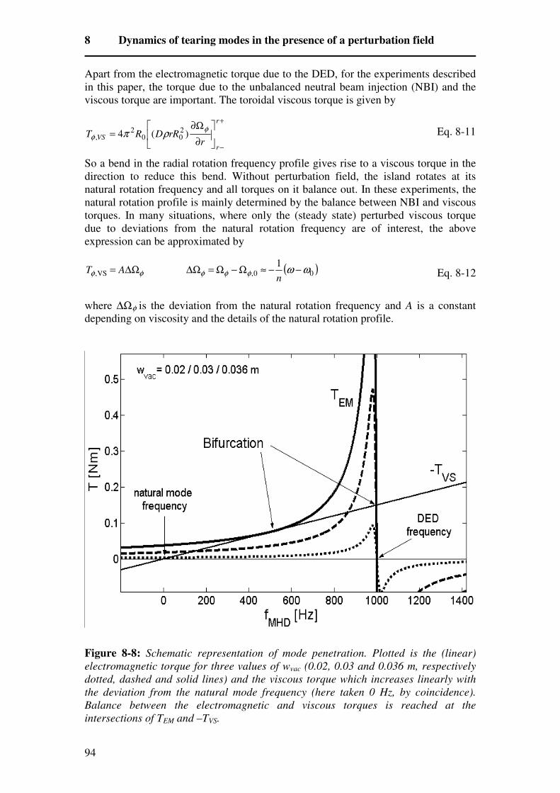
8 Dynamics of tearing modes in the presence of a perturbation field
94
Apart from the electromagnetic torque due to the DED, for the experiments described
in this paper, the torque due to the unbalanced neutral beam injection (NBI) and the
viscous torque are important. The toroidal viscous torque is given by
Eq. 8-11
So a bend in the radial rotation frequency profile gives rise to a viscous torque in the
direction to reduce this bend. Without perturbation field, the island rotates at its
natural rotation frequency and all torques on it balance out. In these experiments, the
natural rotation profile is mainly determined by the balance between NBI and viscous
torques. In many situations, where only the (steady state) perturbed viscous torque
due to deviations from the natural rotation frequency are of interest, the above
expression can be approximated by
Eq. 8-12
where ∆Ωφ is the deviation from the natural rotation frequency and A is a constant
depending on viscosity and the details of the natural rotation profile.
Figure 8-8: Schematic representation of mode penetration. Plotted is the (linear)
electromagnetic torque for three values of wvac (0.02, 0.03 and 0.036 m, respectively
dotted, dashed and solid lines) and the viscous torque which increases linearly with
the deviation from the natural mode frequency (here taken 0 Hz, by coincidence).
Balance between the electromagnetic and viscous torques is reached at the
intersections of TEM and –TVS.
+
−
∂
Ω∂=
r
r
VSr
rRDRTφ
φ ρπ )(4 200
2,
( )00,VS,
1ωωφφφφφ −−≈Ω−Ω=∆Ω∆Ω=
nAT

Imaging and Control of Magnetic Islands in Tokamaks
95
Figure 8-8 shows how the balance between the electromagnetic and viscous torques
leads to mode penetration when the perturbation field strength is gradually increased.
Balance between the electromagnetic and viscous torques is reached at the
intersections of TEM and –TVS. The situations for wvac=0.03 and 0.036 m show two
stable balance points. For wvac>0.036 m, only one remains at fDED=1 kHz. So, starting
at the natural mode frequency, with increasing perturbation field strength (increasing
wvac), the balance point shifts in the direction of the perturbation field frequency. A
critical point is reached when the viscous curve becomes tangent to the
electromagnetic curve. In the linear theory this happens when the difference between
mode and perturbation field frequencies is reduced to half of its natural value (2/5 for
the non-linear theory). If the perturbation field strength is further increased, balance
between the viscous and electromagnetic torques can only be achieved for fMHD=fDED.
This bifurcation is referred to as mode penetration.
8.3.4 Complications
There are a few effects that have to be taken into account to explain the experimental
data that complicate the above general theory. First, the DED perturbation field does
not solely exist of the 2/1 field component. Even though we are most interested in the
dynamics of the observed 2/1 island, also the large 3/1 and 1/1 components of the
DED field have a large influence (on the velocity profile), and have to be taken into
account. The intrinsic error field of TEXTOR is neglected. It is assumed that the
rotation frequency of the islands is always large enough for the torques due to this
field to be negligible. The fact that the islands do not lock to the wall after switch off
of the DED supports this assumption.
Second, a coupling between the 2/1 mode and a mode at the q=1 surface is suggested
by the CXRS data (Figure 8-5). This coupling is present during the unlocking, but not
during the mode penetration. Both the electromagnetic torques on the various rational
surfaces, and the mode coupling, can only be implemented by modelling the velocity
profile. This also enables to model the viscosity realistically.
Third, there is another (type of) torque associated with the perturbation field of the
DED, caused by the near field effects close to the plasma edge [Finken 2005], [Busch
2006]. This torque, acting at the plasma edge, is responsible for the initial increase in
toroidal ion rotation just before penetration, seen in Figure 8-5. It raises the entire
natural rotation profile. In this paper, for simplicity, this torque is neglected. Only the
natural mode rotation frequency is corrected for the influence of this torque.
8.4 Comparison of experiment with theory
The theory described in the last paragraph has little or no free parameters; a
consequence of the fact that they are almost directly derived from first principles like
Maxwell’s equations. All uncertainties are related to the exact plasma properties. To
compare the theory with experiment, it is hence of crucial importance that the
knowledge of the plasma parameters, mainly of the velocity profile, is as accurately as
possible. To model the velocity profile as accurately as possible, a numerical

8 Dynamics of tearing modes in the presence of a perturbation field
96
simulation is used. After describing this simulation, the various stages of the
experiment, being mode penetration, mode growth and mode unlocking, will be
compared to theory.
8.4.1 The numerical simulation
A numerical simulation is used to model the experiment as closely as possible. The
simulation evaluates the evolution of the 2/1 island width and phase, as well as the
velocity profile, including the viscous, electromagnetic (on q=1, 2 and 3) and NBI
torques.
The 2/1 island is treated as a non-linear island (so as an island that rotates at the same
velocity as the plasma), using the Rutherford equation (Eq. 8-2) to determine the
evolution of the island width, and Eq. 8-3 to determine the electromagnetic torque on
the island. Early in the penetration process, the island is smaller than the linear layer
width, and should actually be modelled using the linear theory (Eq. 8-7). During the
important phase of the penetration however, close to the threshold, the 2/1 island is
about 2 cm wide and clearly larger than the linear layer. Treating the island as a non-
linear island throughout the entire penetration doesn’t introduce a large error. The
torque on the q=1 and 3 surfaces on the other hand are evaluated using the linear
theory (Eq. 8-7), assuming ∆’ for the 1/1 and 3/1 modes is negative enough to prohibit
a growth of these modes into the non-linear regime.
The modelled velocity profile (see Figure 8-9) is based on the toroidal ion rotation
profile, as (partly) measured by CXRS. The natural profile is determined by balancing
the neutral beam torque against viscosity. The neutral beam torque is known, and is
about 0.2 Nm. The power deposition profile is assumed to be a Gaussian with full
width at half maximum of 20 cm, centred on the magnetic axis. Good agreement
between the simulated and experimentally measured natural rotation profiles is
reached by taking the momentum diffusion coefficient D=1 m2/s (assumed constant
for the entire plasma), using Eq. 8-11 for the viscous torque.
Table 8-1 lists the input parameters used in the simulation. They are determined using
the measured density and temperature profiles, as well as the estimated current
profile. The latter is estimated from the temperature profile (and loop voltage)
assuming neoclassical resistivity. The time increment used in the simulation is 6105 −⋅ s and the radial resolution of the simulated velocity profile about 0.02 m.
Taking either a significantly (twice) smaller radial resolution, or a significantly larger
time increment, results in numerical instability. The 2/1 island is treated as a rigid
rotator of width w.
The resonant ion rotation frequencies depend on the diamagnetic drift frequency, and
are generally different for q=1, 2 and 3.
Eq. 8-13 *,e
DED,res 2 qq f
n
m
nπ
ω+−=Ω

Imaging and Control of Magnetic Islands in Tokamaks
97
The flat rotation profile measured by CXRS suggests an equal resonant frequency for
q=1 and 2. The resonance for the q=3 surface is not measured, and hence a free
parameter in the simulation 3*e2,1,res3,res )(2 mf∆−Ω=Ω π .
Figure 8-9: Schematic representation of the simulated ion rotation profile, and the
various torques acting on it. The upper solid profile (1) represents the natural profile
determined by the balance between the NBI and viscous torques in the absence of a
mode, with the q=2 surface rotating at Ω0. The 2/1 tearing mode is treated as a rigid
rotator of width w, resulting in the natural rotation profile (2) in the presence of a
mode. The DED perturbation field exerts electromagnetic torques TEM,q on the q=1, 2
and 3 surfaces. Profile (3) shows the situation where only the 2/1 mode is locked to
the DED. Profile (4) (dashed) shows all surfaces locked. The observed mode coupling
between the modes at the q=1 and 2 surfaces is qualitatively taken into account by
introducing two equal but opposite torques T1,2=-T2,1 on the q=1 and 2 surfaces.
Table 8-1 Input parameters of the numerical simulation for the q=1, 2 and 3 surfaces.
q rs [m] C [T] wvac [m] τR [s] s0rec r∆′τ [s]
1 0.105 0.043 0.06 0.24 0.013
2 0.285 0.09 0.04 0.4 0.0083
3 0.375 0.084 0.04 0.13 0.0024
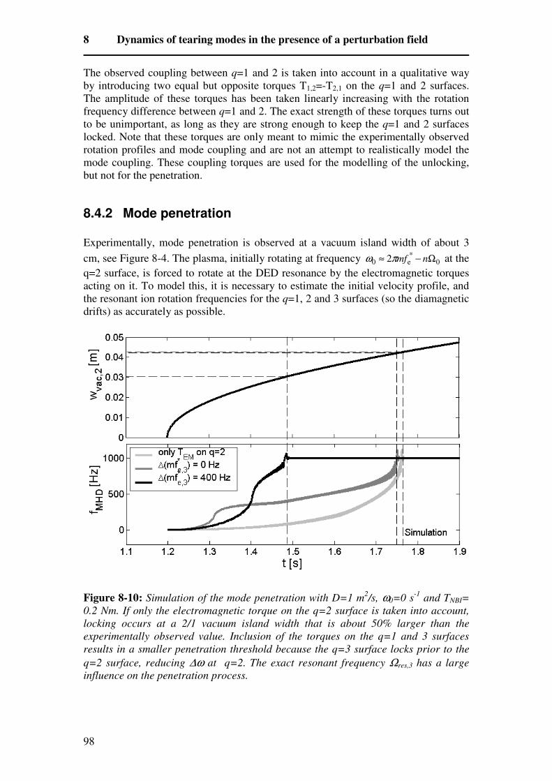
8 Dynamics of tearing modes in the presence of a perturbation field
98
The observed coupling between q=1 and 2 is taken into account in a qualitative way
by introducing two equal but opposite torques T1,2=-T2,1 on the q=1 and 2 surfaces.
The amplitude of these torques has been taken linearly increasing with the rotation
frequency difference between q=1 and 2. The exact strength of these torques turns out
to be unimportant, as long as they are strong enough to keep the q=1 and 2 surfaces
locked. Note that these torques are only meant to mimic the experimentally observed
rotation profiles and mode coupling and are not an attempt to realistically model the
mode coupling. These coupling torques are used for the modelling of the unlocking,
but not for the penetration.
8.4.2 Mode penetration
Experimentally, mode penetration is observed at a vacuum island width of about 3
cm, see Figure 8-4. The plasma, initially rotating at frequency 0*e0 2 Ω−≈ nmfπω at the
q=2 surface, is forced to rotate at the DED resonance by the electromagnetic torques
acting on it. To model this, it is necessary to estimate the initial velocity profile, and
the resonant ion rotation frequencies for the q=1, 2 and 3 surfaces (so the diamagnetic
drifts) as accurately as possible.
Figure 8-10: Simulation of the mode penetration with D=1 m2/s, ω0=0 s
-1 and TNBI=
0.2 Nm. If only the electromagnetic torque on the q=2 surface is taken into account,
locking occurs at a 2/1 vacuum island width that is about 50% larger than the
experimentally observed value. Inclusion of the torques on the q=1 and 3 surfaces
results in a smaller penetration threshold because the q=3 surface locks prior to the
q=2 surface, reducing ∆ω at q=2. The exact resonant frequency Ωres,3 has a large
influence on the penetration process.

Imaging and Control of Magnetic Islands in Tokamaks
99
Figure 8-10 shows the results of the simulation for three different situations. First, the
simulation is done using only the electromagnetic torque on the q=2 surface. The
natural rotation profile is determined by taking D=1 m2/s, TNBI=0.2 Nm, and ω0 = 0 s
-
1. With increasing perturbation field strength, it is seen that the rotation frequency of
the q=2 surface approaches the DED frequency (1 kHz), finally locking to it at a
vacuum island width of about 4.3 cm, significantly higher than the experimental
threshold. An earlier penetration would of course have been observed with a higher ω0
or a smaller momentum diffusion coefficient. To reproduce the observed early
penetration however, unrealistic values of (one of) these two parameters would be
required. So more likely is that the electromagnetic torques on the q=1 and 3 surfaces
play a role in the penetration. To include these two torques, the resonant ion rotation
frequencies Ωres,1 at the q=1 and Ωres,3 at the q=3 surface have to be estimated. The
resonant frequency for the q=1 surface is taken equal to the q=2 surface resonance
(from CXRS). Figure 8-10 shows the results for two different resonant frequencies of
the q=3 surface. Both cases show the locking of the q=3 surface prior to the locking of
the q=2 surface. The locking of the q=3 surface affects the rotation frequency of the
q=2 surface, bringing it closer to resonance, and hence decreasing the penetration
threshold for the q=2 surface. The exact resonant frequency Ωres,3 has a large
influence on the relative timing of the locking of q=2 and 3 surfaces. Although the
exact value of this resonance is unknown, all likely values led to a locking of the q=3
surface in the simulation.
The torque on the q=1 surface turned out to be too small to lead to a locking of the
q=1 surface, due to the large difference between natural and resonant rotation
frequencies. So, only the torque due to the DED perturbation field is (at least in the
simulation) not sufficient to explain the observed mode coupling. A direct coupling
between the mode at the q=1 surface and the (1/1 component of the) 2/1 island is
hence likely.
8.4.3 Mode growth
After the rotation frequency of the q=2 surface has locked to the DED frequency, the
2/1 island can grow to its saturated width. This island growth is governed by the
modified Rutherford equation (Eq. 8-2). The various torques and the velocity profile
do not play a significant role in this process, except for keeping the rotation of the q=2
surface locked.
Figure 8-11 shows both the experimental and simulated evolution of the 2/1 island
width plotted against (t-tpen). Here, the time of penetration tpen is defined as the time
where fMHD reaches fDED (and the phase difference between plasma and vacuum
islands reaches steady state). The simulation shows the oscillation in island width
before penetration, characteristic for the non-linear theory. The island is dragged in
and out of phase with the vacuum island by the difference in rotation frequency. For
an island to be observed by ECE, it has to be larger than a critical width, determined
by the competition between perpendicular and parallel transport, which for TEXTOR
is of the order of 2 cm [Fitzpatrick 1995]. So, the fact that the oscillations are not
observed experimentally doesn’t mean they are not there.

8 Dynamics of tearing modes in the presence of a perturbation field
100
Directly after penetration, which happens at a relatively large perturbation field
amplitude, the phase difference between plasma and vacuum islands settles at a value
close to zero. As the plasma island grows, the phase difference approaches zero even
closer, because the electromagnetic torque increases quadratically with both plasma
and vacuum island widths. But as long as the phase difference remains close to zero, it
doesn’t significantly influence the 2/1 mode growth. The two important parameters in
the modified Rutherford equation are the current diffusion time τR (which is
estimated, see Table 8-1), and the unknown stability parameter ∆’. In the simulation
shown, ∆’ is neglected, except for island widths exceeding 0.1 m where ∆’ has been
taken slightly negative to reproduce the observed saturated island width of 0.11 m (the
same ∆’ is used as was found in the analysis of chapter 9). For small plasma islands,
∆’ can safely be neglected, as the perturbation field term of the Rutherford equation
then dominates over the ∆’ term. For larger island widths, ∆’ does significantly
influence the island growth after penetration, finally (in these experiments) leading to
saturation. The fact that before switching on the DED, no natural island was present
(hence negative ∆’), while after switching off the DED the island remains with an
almost unaltered width of around 0.1 m (and hence ∆’(w)=0 for w=0.1m), it is
assumed that ∆’ is close to zero during the entire process. The above observations are
however hard to explain without an evolution of ∆’ (as a function of w) during
penetration. Despite neglecting ∆’ however, Figure 8-11 shows reasonable agreement
between experiment and simulation.
Figure 8-11: Comparison of the experimentally observed 2/1 island growth during
penetration (#99175) with the simulation (using the non-linear theory). The time of
penetration tpen is defined as the time at which the rotation frequency has reached the
resonant value. The simulation shows oscillations in w prior to locking (with
maximum amplitude w0), characteristic for the non-linear theory. In the simulation,
∆’ is neglected for w < 0.1 m, and slightly negative for larger islands, to reproduce
the observed saturated island width.

Imaging and Control of Magnetic Islands in Tokamaks
101
8.4.4 Mode unlocking
During the locked phase (at full DED current), where the 2/1 island has its saturated
island width, the phase difference between the plasma and vacuum islands is close to
zero. The electromagnetic torque, which is linearly proportional to this phase
difference (for small angles), settles at the value needed to balance all other torques on
the 2/1 island. The maximum possible electromagnetic torque, at ∆(mξ) = π/2, is
however much larger. During the ramp down of the DED current, the torque balance
on the 2/1 island can hence be maintained by gradually increasing the phase
difference, keeping the electromagnetic torque constant. Unlocking occurs when the
phase difference has reached π/2, and the maximum electromagnetic torque is needed
to balance all other torques (assuming the plasma island width stays the same,
otherwise unlocking occurs already at a smaller angle, see [Fitzpatrick 1993]).
After unlocking, the electromagnetic torque is not sufficient anymore to keep torque
balance, and the island rotation will start to deviate from the DED frequency (in the
direction of the natural MHD frequency). Due to this frequency mismatch the
remaining electromagnetic torque will rapidly loose influence, leaving the plasma free
to relax back to the natural rotation profile. The initial rate of change of the 2/1
rotation frequency is determined by the sum of the torques on the island just after
unlocking, which is equal but opposite to the electromagnetic torque that was still
present just before unlocking. So the value of dω/dt just after unlocking is a direct
measure for the electromagnetic torque during the entire locked phase, and in
particular the maximum electromagnetic torque (sin(∆(mξ))=1) at the moment of
unlocking. The smaller the value of dω/dt after unlocking, the less the plasma opposes
the locked state (either because the natural rotation is closer to the DED resonance or
because viscosity is smaller), the easier the island can be kept locked by the
perturbation field. So, as the perturbation field strength depends linearly on the DED
coil current amplitude, a linear dependency between the observed dω/dt and the
threshold IDED for unlocking is expected. Figure 8-12 shows the MHD frequency
during unlocking for four discharges. Although all discharges had identical settings, a
variation in natural mode frequency and initial dω/dt is observed. As expected, the
discharge with the largest dω/dt unlocks first, and the DED current at unlocking scales
approximately linear with the observed dω/dt.
The difference in natural MHD frequency for the four discharges shown, might be
caused by a difference in the momentum diffusion coefficient. Although only a factor
of two variation in ∆Ω is observed in Figure 8-12, the variation in the observed dω/dt
is about a factor of four. As a linear scaling of the viscous torque with ∆Ω is expected
(see Eq. 8-12), this suggest a variation in momentum diffusion coefficient, the
discharge with the highest dω/dt having a twice as high viscosity. Regardless of the
value for D however, the initial dω/dt is still a direct measure for the torque imbalance
after unlocking, see Eq. 8-10. For a direct application of this equation to the 2/1 island
it is however not a priori clear which mass has to be taken (some ‘effective’ island
mass, including the shell of plasma surrounding the island that moves along due to
viscosity). The numerical simulation doesn’t have this problem, because the entire
velocity profile is modelled, applying Eq. 8-10 to each radial increment of the velocity
profile using their actual mass (from the measured density profile).

8 Dynamics of tearing modes in the presence of a perturbation field
102
Figure 8-12: a) The experimentally observed MHD frequency during unlocking for
four identical TEXTOR discharges and b) the corresponding DED current. The
almost instantaneous drop to a large negative dω/dt during unlocking is due to the
loss of the electromagnetic torque. The value of dω/dt just after unlocking is a
measure for the (viscous) torque on the 2/1 island, and is equal in amplitude to the
electromagnetic torque just before unlocking. The discharge with the largest viscous
torque unlocks first. c) As expected, the DED current at unlocking scales
approximately linearly with the viscous torque.
Figure 8-13 shows the results of the numerical simulation for the unlocking phase.
Use has been made of the experimental DED current (vacuum island width), D=1
m2/s, ω0=0 s
-1, TNBI= 0.2 Nm and ∆(mfe
*)3=0 Hz as input parameters. The coupling
a)
c)
b)

Imaging and Control of Magnetic Islands in Tokamaks
103
between the modes at the q=1 and 2 surfaces is mimicked by the inclusion of two
opposing torques. The simulation shows the expected increase in phase difference
before unlocking (the wiggle is due to the step in the vacuum island width), and the
resulting relaxation of the MHD frequency after unlocking (when the phase difference
passes π/2). The time trace of the electromagnetic torque on the q=2 surface shows a
more complex picture, with steps in the torque corresponding to the unlocking of one
of the resonant q surfaces. First, the q=1 surface is seen to ‘unlock’, leading to a larger
torque on the q=2 surface. Note that the coupling between the q=1 and 2 modes
remains. The rotation frequency of the q=1 surface (almost) doesn’t change, but the
DED torque on the q=1 surface becomes negligible. The unlocking of the q=3 surface
leads to a decrease in torque on the q=2 surface (transition of the dotted profile to
profile 3 in Figure 8-9), resulting in a small bump on the phase difference time trace.
Because of the large island width (hence large electromagnetic torque) the 2/1 mode is
the last to unlock. So, just before unlocking only the electromagnetic torque on the 2/1
mode has to be taken into account. After unlocking, the electromagnetic torque on the
2/1 mode is seen to oscillate around zero, increasing in frequency as ∆ω increases.
Figure 8-13: Simulation of the mode unlocking with D=1 m2/s, ω0=0 s
-1, TNBI= 0.2
Nm and ∆(mfe*)3=0 Hz including the coupling between the modes at the q=1and 2
surfaces. Use has been made of the experimentally observed vacuum island width.
Unlocking of the 2/1 island occurs when the phase difference between plasma and
vacuum islands exceeds π/2. Prior to the unlocking of the 2/1 island, both the q=1 and
3 surfaces unlock (although q=1 stays coupled to q=2), as can be seen from the steps
in TEM,2. The electromagnetic torque on the 2/1 island prior to unlocking is about 0.1
Nm. After unlocking, the torque oscillates around zero. The loss of these 0.1 Nm
results in a dω/dt of about 5101⋅ s-2
.

8 Dynamics of tearing modes in the presence of a perturbation field
104
Figure 8-14 shows the experimental MHD frequency and phase difference during
unlocking. The expected increase in phase difference and subsequent frequency
relaxation are observed. The behaviour of the q=1 and 3 surfaces can not be seen from
this data (although the small bump on the phase difference, better seen in Figure 8-4,
might correspond to the unlocking of the q=3 surface). The simulation however shows
that it is safe to assume that the q=2 surface is the last to unlock.
Figure 8-14: Experimental MHD frequency and phase difference during unlocking
(#99175). After unlocking, a dω/dt of about 5102 ⋅ s-2
is observed. According to the
numerical simulation this corresponds to a viscous torque of about 0.2 Nm. The
dashed line in the lower graph is the theoretical phase difference expected in a steady
state situation, calculated from Eq. 8-3 using TEM=0.2 Nm and the experimental
values for w and wvac.
To link the observed dω/dt of about 5102 ⋅ s-2
to a torque (using Eq. 8-10), the
‘effective’ island mass has to be known. In the numerical simulation, where this
problem is avoided, the observed dω/dt was about 5101⋅ s-2
, and corresponded to a
torque of about 0.1 Nm (see Figure 8-13). This suggests that the experimentally
observed dω/dt of about 5102 ⋅ s-2
corresponds to a torque of about 0.2 Nm. The dotted
line in Figure 8-14 gives the theoretically expected steady state phase difference,
calculated with Eq. 8-3, using TEM=0.2 Nm and the experimental values for w and
wvac. This curve is indeed very close to the experimental one, predicting the unlocking
only slightly too early.
Remember that the phase difference during the ‘strongly’ locked phase was
synthetically set to zero, and hence the entire curve might be shifted up or down.

Imaging and Control of Magnetic Islands in Tokamaks
105
Experimentally, only the change in phase difference is measured, which is in
agreement with the theoretically observed change.
8.5 Summary and discussion Although the exact details of the experiment are hard to reconstruct, theory and
experiment agree, qualitatively and to a large extent also quantitatively, on all
accounts. The sudden growth of an island during penetration, and the sudden torque
imbalance (leading to a stepwise change in dω/dt) during unlocking are reproduced.
Moreover, these bifurcations are observed at threshold perturbation field amplitudes
close to the theoretical values, the threshold for unlocking being much smaller than
the one for penetration. The predicted change in phase difference between plasma and
vacuum islands before unlocking is actually observed, and in agreement with the
(viscous) torque on the island, derived from the frequency relaxation after unlocking.
Smaller viscous torques led to smaller thresholds for unlocking, approximately linear
with the DED coil current amplitude. Only taking account of the electromagnetic
torque on the q=2 surface in the numerical simulation led to a threshold for 2/1 mode
penetration of about 50% higher than experimentally observed. Inclusion of the
electromagnetic torque on the q=1 and, in particular, the q=3 surface, resulted in a
significantly lower penetration threshold. The observed threshold is most likely
explained by the locking of the q=3 surface prior to, or simultaneous with, the q=2
surface. Finally, despite the unknown island stability parameter ∆’, the growth of the
2/1 island after penetration is well reproduced in the numerical simulation.
Some questions remain. The 2/1 island is observed to be stable (negative ∆’) before
the DED is switched on, but it doesn’t disappear after switching off the DED. A
threshold island width (as is the case for neoclassical tearing modes), might explain
this. It is, however, unlikely that the 2/1 island is of neoclassical nature, due to the
small bootstrap current fraction in these experiments. An evolution of the current
profile leading to a less stable island is also hard to imagine. A growing island uses
the free energy available in the current profile and should hence lead to a more stable
current profile. Probably the stability has changed due to the coupling with the mode
at the q=1 surface, making the combined 2/1-1/1 system more unstable than the
individual modes. Luckily, the theoretical predictions are not very sensitive to the
exact value of ∆’ (for ∆ω>>1/τrec, ∆’ can even safely be neglected). The results of the
numerical simulation are however very sensitive to, in particular, the chosen values
for ω0, Ωres,3 and wvac, leaving some room for variation.
The way the mode coupling between the 2/1 island and the mode at the q=1 surface is
treated in the simulation is very qualitatively. Simply, two (strong enough) torques are
introduced to mimic the observed velocity profile. It turns out however, that this
coupling doesn’t significantly affect the dynamics of the 2/1 island. The net torque the
2/1 island ‘feels’, is not changed by the inclusion of the two (cancelling) torques
responsible for the coupling. A more realistic treatment of the mode coupling is hence
beyond the scope of this thesis.
Finally, the question remains whether there actually are 1/1 and 3/1 modes in the
plasma. Experimentally, no 3/1 mode is observed. The existence of a 1/1 mode is less
important for the results presented in this paper, but is likely because of the observed

8 Dynamics of tearing modes in the presence of a perturbation field
106
coupling. For an island to be experimentally observable (by for instance ECE), it
should be large enough to affect the pressure profile. Its width has to be larger than a
critical width, determined by the competition between perpendicular and parallel
transport, which for TEXTOR is of the order of 2 cm [Fitzpatrick 1995]. In the
simulation it is assumed that the ∆’ for these modes is negative enough to prohibit a
growth of these modes into the ‘non-linear’ regime. So, the electromagnetic torques
do not rely on the existence of an experimentally observable island. If, in reality, there
are larger 1/1 or 3/1 islands (∆’ less negative than assumed), then the role of the
electromagnetic torques on these islands (scaling with w2) is underestimated, and the
non-linear theory might have been necessary. Again, during penetration, the value of
∆’ is relatively unimportant as normally ∆ω>>1/τrec.
Despite these questions regarding the details of the experiment, one can conclude that
the theory (as mainly developed by Fitzpatrick) worked remarkably well to explain
the observations, throughout the various stages of the experiment (mode penetration,
growth and unlocking), both qualitatively and quantitatively. This gives confidence in
the validity of predictions based on this theory, like for instance the tolerable error
field in future devises like ITER. One should however make sure to include all
important details of the experiment in question into the analysis. The experiments
described here showed for instance, that in order to describe the behaviour of the q=2
island, it was essential to include the effect of the other rational surfaces in the
plasma.
Imaging and Control of Magnetic Islands in Tokamaks
107
9 The effect of heating on the suppression of tearing modes
*
I.G.J. Classen1, E. Westerhof
1, C.W. Domier
2, A.J.H. Donné
1, R.J.E. Jaspers
1,
N.C. Luhmann Jr.2, H.K. Park
3, M.J. van de Pol
1, G.W. Spakman
1,
M.W. Jakubowski4 and TEXTOR team
4
1 FOM-Institute for Plasma Physics Rijnhuizen, Association EURATOM-FOM, PO
Box 1207, 3430 BE Nieuwegein, The Netherlands, www.rijnh.nl#
2 University of California at Davis, Dept. of Applied Science, Davis, California,
95616 U.S.A. 3 Princeton Plasma Physics Laboratory, Princeton, New Jersey, 08543 U.S.A.
4 Forschungszentrum Jülich GmbH, Institut für Plasmaphysik, Association
EURATOM-FZJ, D-52425 Jülich, Germany#
#Partners in the Trilateral Euregio Cluster
Abstract. The suppression of (Neoclassical) Tearing Modes is of great
importance for the success of future fusion reactors like ITER. Electron
cyclotron waves can suppress islands, both by driving non-inductive current
in the island region and by heating the island, causing a perturbation to the
Ohmic plasma current. This Letter reports on experiments on the TEXTOR
tokamak, investigating the effect of heating, which is usually neglected. The
unique set of tools available on TEXTOR, notably the Dynamic Ergodic
Divertor to create islands with a fully known driving term, and the electron
cyclotron emission imaging (ECE-Imaging) diagnostic to provide detailed
2D electron temperature information, enables a detailed study of the
suppression process and a comparison with theory.
52.55.Tn, 52.55.Fa, 52.25.Fi, 52.70.Gw
Tearing modes, and in particular neoclassical tearing modes (NTMs), have a
deleterious effect on the performance and stability of tokamak plasmas. Larger
tokamaks, like the proposed ITER tokamak, are more susceptible to the formation of
NTMs. It is therefore important to develop techniques to control or suppress them and
to gain understanding of the suppression process. Islands can be stabilized by driving
a (helical) current perturbation inside the island region. Gyrotrons are an ideal tool for
the localized generation of this current through the injection of radio frequency waves
* The work presented in this chapter is published in this form in Physical Review Letters under the title
‘Effect of heating on the suppression of tearing modes in tokamaks’.
I.G.J. Classen et al., Phys. Rev. Lett. 98, 035001 (2007)

9 The effect of heating on the suppression of tearing modes
108
into the plasma. This current can either be directly driven non-inductively by Electron
Cyclotron Current Drive (ECCD) [La Haye 2006] or indirectly by heating the island
by Electron Cyclotron Resonance Heating (ECRH) ([Hoshino], [Sing 1993], [Kislov
1997]), causing a helical perturbation to the Ohmic current due to the temperature
dependence of the plasma conductivity. ECCD is thought to be a more efficient way
to suppress (neoclassical) islands. The tearing mode suppression by heating is often
neglected. In this Letter, it will be shown that on TEXTOR the physical mechanism at
work during heating can be clearly identified. It is demonstrated that also heating
gives a sizeable suppression of the islands.
A set of tearing mode suppression experiments on the TEXTOR tokamak is described,
that focuses on the suppression by heating (ECRH). In TEXTOR, suppression by
ECRH dominates over ECCD [Westerhof 2006] due to the low current drive
efficiency (low Te).
TEXTOR is a medium sized limiter tokamak with a circular plasma cross section
(R0=1.75 m, a=0.46 m) and is ideally suited for island suppression studies due to the
unique combination of available tools. With the Dynamic Ergodic Divertor [Special
Issue 1997], islands can be created and controlled with (in contrast to other tokamaks)
a fully known driving term. The gyrotron can be used to apply highly localized
heating or current drive inside the island. Finally, the process of suppression can be
observed in detail by the 2D electron cyclotron emission imaging (ECE-Imaging)
diagnostic [Park 2003].
Figure 9-1: Overview of a typical discharge. a) DED vacuum magnetic field. b) Te
time trace from an ECE-Imaging channel just inside the island. c) Amplitude of the
DED coil currents. d) Ohmic power and ECRH power.
The Dynamic Ergodic Divertor (DED) on TEXTOR is a perturbation field experiment
consisting of 16 helical coils on the high field side, aligned with the q=3 field lines.
Figure 9-1a shows the vacuum field used for the experiments described in this Letter,
containing large 3/1 and 2/1 island chains. In the presence of a plasma, the magnetic
topology changes due to shielding currents that are generated on the rational q

Imaging and Control of Magnetic Islands in Tokamaks
109
surfaces. For these experiments, this results in a plasma in which only a 2/1 island is
destabilized when the current in the DED coils exceeds a threshold [Koslowski 2006].
In the underlying work, 1 kHz AC DED currents are used, resulting in a poloidal
rotation of 500 Hz for the m/n = 2/1 island which is locked to the rotating perturbation
field.
An 800 kW, 140 GHz gyrotron is used to suppress the islands. The steerable launcher
enables accurate positioning of the power on the resonant surface rs (at the high field
side for these experiments). Both continuous (CW) and modulated power is possible.
The radial width of the (assumed Gaussian) power deposition profile is calculated to
be 1.5 cm full width at half maximum.
The ECE-Imaging diagnostic on TEXTOR measures the electron temperature in a 2D
array of 8 (radially) by 16 (vertically) observation volumes in the poloidal plane,
representing about 8 by 16 cm2 in the plasma, centred on the equatorial plane. For
these experiments, the field of view was adjusted to the q=2 surface at the low field
side, and the data were sampled at 200 kHz.
Figure 9-1 gives an overview of a typical discharge. All discharges have a toroidal
magnetic field of 2.25 T, a toroidal plasma current of 300 kA and a line averaged
density of about 3.10
19 m
-3. The DED coil current amplitude is ramped up, reaching a
flat top of 2 kA (Figure 9-1c). A 2/1 tearing mode is destabilized when the DED
current becomes sufficiently high, as can be seen on an ECE-Imaging temperature
time trace from a channel just inside the island radius as a 1 kHz oscillation (Figure
9-1b). From 2.2 s to 2.9 s, ECRH is switched on (Figure 9-1d), either CW or
modulated, with (for these experiments) 200, 300 or 400 kW of power. These power
levels are comparable to the Ohmic input power. In this Letter, only data are
presented for which the ECRH power was deposited directly on the resonant q=2
surface. The appropriate launcher position is determined from a scan of the poloidal
launcher angle, searching for optimum island suppression [Westerhof 2006].
For comprehensive visualization of the ECE-Imaging data, a poloidal reconstruction
is used in which the data for one full rotation period are mapped onto a poloidal shell,
assuming rigid plasma rotation. Note that the poloidal reconstruction only represents
the low field side structure of the island. Figure 9-2 shows the reconstruction of the
island during the three main stages of the suppression process. The first stage (Figure
9-2a) is the situation in which the island has been generated and has reached a
saturated width of about 12 cm, but before ECRH application. In this phase, the
temperature profile inside the island is still flat. The hot, central plasma,
approximately elliptically deformed by the island, is clearly visible. The second
reconstruction (Figure 9-2b), at about 10 ms after switch on of ECRH, shows a
peaked Te profile inside the island. Although an island degrades the global
confinement of the plasma, the island itself can confine energy and particles. The third
stage (Figure 9-2c) is the steady state situation long (more than 100 ms) after switch
on of ECRH. The island is now suppressed to about half the initial size, the central
plasma is less deformed and the peaked temperature region inside the island is
narrower.
An automated algorithm is used to extract the main island parameters from the
reconstructed ECE-Imaging data. To determine the full island width w, an ellipse is
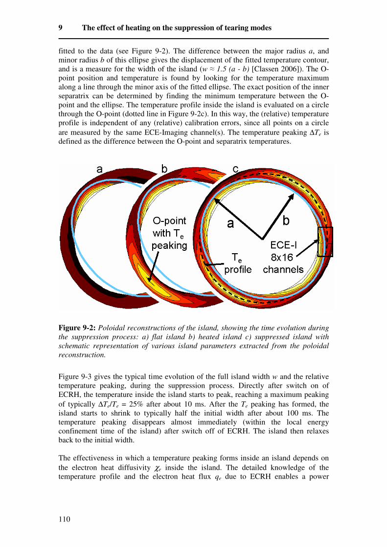
9 The effect of heating on the suppression of tearing modes
110
fitted to the data (see Figure 9-2). The difference between the major radius a, and
minor radius b of this ellipse gives the displacement of the fitted temperature contour,
and is a measure for the width of the island (w ≈ 1.5 (a - b) [Classen 2006]). The O-
point position and temperature is found by looking for the temperature maximum
along a line through the minor axis of the fitted ellipse. The exact position of the inner
separatrix can be determined by finding the minimum temperature between the O-
point and the ellipse. The temperature profile inside the island is evaluated on a circle
through the O-point (dotted line in Figure 9-2c). In this way, the (relative) temperature
profile is independent of any (relative) calibration errors, since all points on a circle
are measured by the same ECE-Imaging channel(s). The temperature peaking ∆Te is
defined as the difference between the O-point and separatrix temperatures.
Figure 9-2: Poloidal reconstructions of the island, showing the time evolution during
the suppression process: a) flat island b) heated island c) suppressed island with
schematic representation of various island parameters extracted from the poloidal
reconstruction.
Figure 9-3 gives the typical time evolution of the full island width w and the relative
temperature peaking, during the suppression process. Directly after switch on of
ECRH, the temperature inside the island starts to peak, reaching a maximum peaking
of typically ∆Te/Te = 25% after about 10 ms. After the Te peaking has formed, the
island starts to shrink to typically half the initial width after about 100 ms. The
temperature peaking disappears almost immediately (within the local energy
confinement time of the island) after switch off of ECRH. The island then relaxes
back to the initial width.
The effectiveness in which a temperature peaking forms inside an island depends on
the electron heat diffusivity χe inside the island. The detailed knowledge of the
temperature profile and the electron heat flux qe due to ECRH enables a power

Imaging and Control of Magnetic Islands in Tokamaks
111
balance analysis. Applied to the island geometry, the standard formula for a steady
state power balance eeee Tnq ∇−= χ can be written as
Eq. 9-1
where S
. denotes a flux surface average. The island flux surface label
( )ξmwrr s cos)(8 22 −−=Ω − (using the helical angle φθξ )/( mn−= ) can be seen as
a radial coordinate inside the island: in the O-point, Ω = -1, on the separatrix, Ω = 1.
Te and χe are assumed to be flux functions. For simplicity, ne is taken constant over
the island. Inside the island, ECRH is the only significant heating source, and is
assumed to be ideally aligned on rs (for modulated power also centred on the O-
point).
Figure 9-3: Typical time evolution of a) relative Te peaking and b) island width.
The numerical evaluation of Eq. 9-1 has been performed in the fully suppressed island
stage of the discharges. Figure 9-4 shows the results of the power balance analysis for
three discharges with different CW ECRH input power (400, 300 and 200 kW). The
temperature profiles for these three powers are shown in Figure 9-4a. The profiles of
the electron thermal diffusivity (Figure 9-4b) show that over the largest part of the
island, χe is about 1 to 1.5 m2/s. Near the O-point, the uncertainty in the exact
positioning of ECRH leads to deviations. Near the separatrix, χe rises due to the fact
that close to the separatrix the electron temperature can no longer be considered a flux
function [Fitzpatrick 1995]. A power balance analysis of the entire plasma reveals that
the transport in the ambient plasma is comparable to the transport inside the island.
For the ambient plasma, χe is typically 1 m2/s inside the deposition radius of ECRH
and somewhat higher outside the deposition radius.
S
eeeSe
d
dTnq Ω∇
Ω−= ⊥,χ

9 The effect of heating on the suppression of tearing modes
112
Figure 9-4: Power balance inside the island for three CW input powers. a)
Temperature profiles inside the fully suppressed islands. Note the large effect the
ECRH power has on the equilibrium (separatrix) temperature. b) Heat diffusion
coefficients inside the islands.
Discharges with modulated ECRH show results very similar to the CW results.
Similar relative temperature peakings and similar transport levels are observed. The
only significant difference is that for modulated ECRH the equilibrium temperature
(so the temperature of the island separatrix) rises less due to the lower total power
input into the plasma. Consequently, modulation has advantages, since it doesn’t spill
power outside the island and disturbs the plasma less. Suppression works as long as
there is power deposited inside the island.
The evolution of a tearing mode depends on the (helical) currents that flow inside the
island region. The time evolution of the island width is governed by Eq. 9-2, relating
the stability parameter ∆’ (the step in the poloidal flux function ψ over the island
region) to the total helical current inside the island region [Wilson 2004].
Eq. 9-2
If only the inductive current due to the growth of the island dw/dt is taken into
account, Eq. 9-2 results in the classical Rutherford equation (Eq. 9-3, skipping the last
two terms) [Rutherford 1973] where w is the full island width and ηµτ /2
0 sr r= is the
current diffusion time. The inclusion of other contributions to the parallel current
results in modifications to the classical Rutherford equation.
For these experiments, two modifications are important. First, a destabilizing
contribution MDED due to the shielding currents caused by the resonant external DED
currents (Eq. 9-4, valid for strongly locked islands) ([Fitzpatrick 1993], [Fitzpatrick
1998], [Morris 1992a]). The DED sets up a perturbed magnetic field resonant with the
island, causing currents to flow inside the island region that try to compensate this
external field. Second, a stabilizing contribution MECRH due to the perturbed Ohmic
current caused by temperature perturbations inside the island (Eq. 9-5) [Hegna 1997].
∫ ∫+
−
=∆′2/
2/
//0 )cos(2~wr
wr
s
s
s
drmjdyR ξξµψ
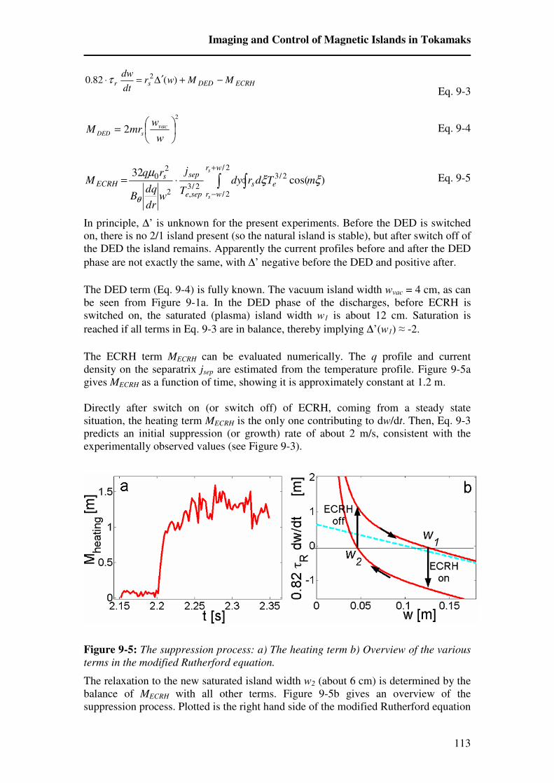
Imaging and Control of Magnetic Islands in Tokamaks
113
Eq. 9-3
Eq. 9-4
Eq. 9-5
In principle, ∆’ is unknown for the present experiments. Before the DED is switched
on, there is no 2/1 island present (so the natural island is stable), but after switch off of
the DED the island remains. Apparently the current profiles before and after the DED
phase are not exactly the same, with ∆’ negative before the DED and positive after.
The DED term (Eq. 9-4) is fully known. The vacuum island width wvac = 4 cm, as can
be seen from Figure 9-1a. In the DED phase of the discharges, before ECRH is
switched on, the saturated (plasma) island width w1 is about 12 cm. Saturation is
reached if all terms in Eq. 9-3 are in balance, thereby implying ∆’(w1) ≈ -2.
The ECRH term MECRH can be evaluated numerically. The q profile and current
density on the separatrix jsep are estimated from the temperature profile. Figure 9-5a
gives MECRH as a function of time, showing it is approximately constant at 1.2 m.
Directly after switch on (or switch off) of ECRH, coming from a steady state
situation, the heating term MECRH is the only one contributing to dw/dt. Then, Eq. 9-3
predicts an initial suppression (or growth) rate of about 2 m/s, consistent with the
experimentally observed values (see Figure 9-3).
Figure 9-5: The suppression process: a) The heating term b) Overview of the various
terms in the modified Rutherford equation.
The relaxation to the new saturated island width w2 (about 6 cm) is determined by the
balance of MECRH with all other terms. Figure 9-5b gives an overview of the
suppression process. Plotted is the right hand side of the modified Rutherford equation
ECRHDEDsr MMwrdt
dw−+∆′=⋅ )(82.0 2τ
2
2
=
w
wmrM vac
sDED
∫ ∫+
−
⋅=2/
2/
2/3
2/3,2
20 )cos(
32wr
wr
es
sepe
sepsECRH
s
s
mTdrdyT
j
wdr
dqB
rqM ξξ
µ
θ

9 The effect of heating on the suppression of tearing modes
114
(equals 0.82 τr dw/dt) against w. The upper curve is composed of the ∆’ and DED
terms. The lower curve includes the heating term (and is hence 1.2 m lower). To
reproduce the observed saturated island widths, a ∆’ term of the form of the dashed
line had to be introduced.
It should be noted that the stabilizing heating term in the Rutherford equation is the
same for Neoclassical Tearing Modes (NTMs) which are driven unstable by the
perturbed bootstrap current instead of the DED ([Fitzpatrick 1995], [Wilson 2004],
[Hegna 1997]). In the presence of an island, the pressure gradient is removed, which
results in a ‘hole’ in the bootstrap current distribution, which gives a destabilizing
contribution to the Rutherford equation. In the ITER reference scenario, bootstrap
current fractions of about 30% are expected [Sips 2005]. Therefore, to compensate
this lost bootstrap current by the extra current due to a peaked temperature inside the
NTM, a temperature peaking of about 20% is needed. In Eq. 9-6 the general scaling
for the temperature peaking is given, assuming narrow islands and a power deposition
width smaller than the island width.
Eq. 9-6
To get a 20% temperature peaking in ITER, Eq. 9-6 requires χe < 0.2 m2/s inside the
ITER islands, assuming 20 MW of ECRH power. Even if inside the ITER islands χe ~
0.5 m2/s, which is equal to the expected equilibrium χe at the q = 3/2 surface in ITER,
the heating effect is still significant, and relaxes the gyrotron power requirements
based only on current drive (ECCD).
This work, supported by the European Communities under the contract of Association
between EURATOM/FOM, was carried out within the framework of the European
Fusion Program together with the US Department of Energy. The views and opinions
expressed herein do not necessarily reflect those of the European Commission.
ees
ECRH
e
e
e
e
s
ECRHeee
TRnr
wP
T
Tw
T
T
Rr
PTnq
χχ ∝
∇∝
∆∝∇−=

Imaging and Control of Magnetic Islands in Tokamaks
115
10 Conclusions and Outlook
Making use of the ideal combination of tools available on TEXTOR, in particular
ECE-Imaging, the DED and the 140 GHz gyrotron, experiments were conducted on
three transport related topics, being magnetic islands, magnetic field perturbations at
the plasma edge and high frequency temperature fluctuations.
To explore the capabilities of the ECE-Imaging diagnostic, experiments on the effects
of a perturbation field on the edge temperature profile, and on high frequency
(temperature) fluctuations were presented. The added value of having a 2D diagnostic
was demonstrated in both these experiments. The edge temperature profile during
DED 12/4 operation showed a pronounced 2D structure, and the measured
fluctuations showed distinctly different behaviour in radial and poloidal directions.
The capabilities of ECE-Imaging as a 2D fluctuation diagnostic were confirmed,
encouraging a more in depth investigation of these topics in the future.
The main results presented in this thesis are the quantitative experimental verifications
of two aspects of the dynamics of magnetic islands: The effects of a perturbation field
and local heating. The known perturbation field of the DED and the accurate local
power deposition of ECRH enabled an experimental verification of the heating and
perturbation field terms in the modified Rutherford equation, governing island
evolution.
10.1 2D structures and fluctuations
In chapter 5, 2D ECE-Imaging measurements of the edge electron temperature during
DED 12/4 operation were presented. The effects on the temperature profile and
transport were investigated.
During DED, the edge temperature profile developed a pronounced 2D structure. A
poloidal asymmetry was observed close to the edge (relatively hot bulges in an
otherwise cold region), but not further into the plasma. The relatively high
temperature structures (bulges) at the edge could be linked to regions of long
connection length (where two ‘fingers’ cross) in the theoretical calculations of the
vacuum field topology (Atlas code). Also, the poloidally asymmetric part of the
plasma could be identified as the laminar zone. Theory and experiment agree on (the
evolution of) the position of these structures, giving confidence in the validity of the
Atlas code, at least in the laminar region.
An overall drop in temperature is observed, which is a clear sign of enhanced
transport. A transport enhancement of about a factor of two (poloidally averaged) in

10 Conclusions and Outlook
116
the poloidally asymmetric region was observed. No notable change in transport in the
poloidally symmetric part of the plasma and the hot bulges was found.
So, the DED has a large influence on the Te profile and heat transport at the plasma
edge. Moreover, a strong dependence of the observed 2D structure on the value of q at
the edge is observed, making the edge structure controllable. These observations
confirm that the DED is a flexible tool to control and investigate the plasma-wall
interaction.
The experimental results on the DED edge structures show that ECE-Imaging is
capable of direct 2D observation of structures in the temperature profile. To reduce
the noise without sacrificing spatial or time resolution, effective use has been made of
a filtering based on singular value decomposition. For high frequency, low amplitude
fluctuations, a direct observation is not possible due to the thermal noise. However, by
using correlation techniques, the time averaged properties of such fluctuation can be
determined. ECE-Imaging enables correlations in both radial and poloidal directions,
making it possible to reveal the 2D structure (propagation speed, wavelength and
correlation length) of fluctuations.
In chapter 6, measurements of two types of high frequency fluctuations in TEXTOR
were presented: the quasi-coherent (QC) mode and the Alfvén-like mode. The
measurements of the QC mode demonstrated that ECE-Imaging is (at least) sensitive
to fluctuations with f <= 100kHz, λ >=0.07m (k<=1cm-1
), and relative amplitude
larger than 0.2%. The following properties of the fluctuations could be derived:
• The amplitude of the QC mode was observed to depend on radius: about 3% at the
edge to below 0.2% in the plasma centre.
• Temperature and density fluctuations were estimated to be comparable in
amplitude for the QC mode.
• The radial and poloidal behaviour of the QC mode was distinctly different.
o Poloidally, the QC mode was seen to propagate with a velocity of about 6
km/s. The poloidal wavelength was about 7cm, and the poloidal mode
number m about 40.
o Radially, the QC mode is not observed to propagate. The radial correlation
length was about 2cm.
• The lifetime of the QC structures was about 1.10
-5s.
• The two frequency branches of the Alfvén-like mode originate from different
minor radii, and are probably related to the q=2 and 3 surfaces.
The question whether the QC mode can be identified as the ITG mode, as suggested
in [Krämer-Flecken 2003], remains open. The measurements resemble measurements
reported in literature from other fusion devises. The poloidal extent of the QC mode
(wavelength of 7cm) is larger than the radial extent (correlation length of about 2cm).
So, if the QC mode is the ITG mode, the radially extended finger-like structures
typical for the ITG mode are not observed. This could, however, be caused by
velocity shearing, decreasing the radial extent of the turbulent cells.
The experiments in chapters 5 and 6 lay the foundation of a more elaborate
experimental investigation of the two topics in the future. Particularly interesting is
the question whether the quasi-coherent mode can be identified as the ion temperature
gradient (ITG) mode.

Imaging and Control of Magnetic Islands in Tokamaks
117
10.2 Magnetic islands
In general, any helical current in the island region, results in a modification to the
Rutherford equation governing the evolution of the island width. The main goal of
chapters 8 and 9 was an experimental check of two modifications to the Rutherford
equation: the perturbation field term and the heating term, representing the effects of
two currents of totally different origin; the shielding current and the perturbed Ohmic
current respectively.
Apart from influencing the evolution of the island width, the shielding current also
results in a torque on the island, balancing against all other (mainly viscous) torques
on the island. Theoretically, the interplay between this torque balance and the
(perturbation field term in the) modified Rutherford equation determines the dynamics
of tearing modes in the presence of an external perturbation field. The experimental
results presented in chapter 8, investigated the processes of mode penetration and
mode unlocking. The experimental observations lead to the following answers to the
questions posed in chapter 1:
• The mode penetration and unlocking are observed. The sudden growth of an
island during penetration, and the sudden change in rotation frequency of the
island during unlocking, are clear signs of the theoretically expected bifurcations.
• The threshold perturbation field amplitudes (for penetration and unlocking) were
close to the theoretically predicted values, the threshold for unlocking being much
smaller than the one for penetration.
• The expected phase difference between plasma and vacuum islands was observed
and changed as predicted. Before unlocking, with decreasing perturbation field
amplitude, the phase difference increased. The unlocking occurred when the phase
difference exceeded 90 degrees.
So the overall conclusion is that theory and experiment agreed, not only qualitatively
but also to a large extent quantitatively. As in theory both the island evolution and the
torque are consequences of a shielding current, these experiments indirectly confirm
the existence of such a current.
In chapter 9, the experiments on tearing mode suppression by local heating were
presented. The modified Rutherford equation predicts that a peaked temperature
profile inside the island works stabilising. The formation of this temperature peaking
is determined by both the amount and distribution of the power being deposited inside
the island, and the heat transport inside the island. The main results in this chapter
were:
• Large relative temperature peakings inside the island of 25% could be reached.
Inside the island, a typical χe of 1.5 m2/s was found, comparable to the ambient
plasma. Both modulated and CW ECRH gave comparable temperature peakings,
however, modulated ECRH disturbed the plasma equilibrium less and spills less
power outside the island separatrix.
• A significant suppression of the DED induced islands, typically to half their initial
width, is observed, The measured suppression rates were consistent with theory.
• Scaling up the results for TEXTOR to ITER, it was concluded that in ITER the
effect of heating is as large as the effect of current drive if χe < 0.2 m2/s inside the
ITER islands. Even if χe ~ 0.5 m2/s, equal to expected equilibrium χe at the q = 3/2
surface in ITER, the heating effect is still significant.

10 Conclusions and Outlook
118
Again, theory and experiment agree. Two totally different sources of helical current in
the island region (shielding and perturbed Ohmic currents) resulted in the expected
influence on island evolution. This does not only give confidence in the two
modification terms tested directly, but also in the general Rutherford theory. If one
knows the helical current inside the island region, Rutherford theory gives the effect
on island evolution.
So the theory can be confidently applied to future fusion devises like ITER, where
both Rutherford theory and shielding current torques play a large role in processes
like:
• Tearing mode penetration due to the stationary error field.
• Locking of existing modes to the stationary error field, possibly leading to a
disruption.
• Suppression of existing (neoclassical) tearing modes by ECRH and/or ECCD.
When driving current with ECCD, one automatically also heats the island. This effect
is not negligible. Using conservative assumptions (equal heat diffusion coefficients
inside and outside the island, for a 10cm island), still a 20% contribution is expected.
This will result in a faster suppression, with less power consumption. Even though
suppression by heating is less effective for small islands, heating alone could (help)
keep NTMs at an acceptably small width.
10.3 Outlook
The work presented in chapters 8 and 9 showed that the influences of a peaked
temperature and perturbation fields on magnetic island are well understood. This
gives confidence in using the theory of these two effects in future fusion devises like
ITER. As ITER has both gyrotrons, and (as every tokamak) an error field, both effects
play a role.
The results presented in chapters 5 and 6, show that the 2D capability of ECE-
Imaging can contribute to these fields of research. A further exploration of these
topics is desirable. In particular, a more elaborate data set on the quasi coherent mode
under various plasma conditions is of interest, as this mode might be the ion
temperature gradient (ITG) mode, which is one of the turbulent modes thought
responsible for the anomalously high transport in tokamaks.
Although ECE-Imaging already proved to be a good tool for 2D temperature
measurements, progress is being made in further improving this diagnostic. The ECE-
Imaging system has recently been upgraded [Domier 2006], increasing its radial
coverage by about 50%. The limited radial coverage of about 7cm in the old setup
was sometimes a disadvantage in the study of larger MHD instabilities like magnetic
islands or the sawtooth crash, as most of the time ECE-Imaging only offered a partial
view of the instability. The new system will hence facilitate the investigation of larger
plasma structures. In particular one can think of:
• Magnetic islands: More accurate determination of the island width and
temperature profile will be possible.
• Sawtooth crash: The behaviour at both sides of the sawtooth inversion radius
(q=1) can be visualised simultaneous.

Imaging and Control of Magnetic Islands in Tokamaks
119
• Edge Localised Modes (ELMs): In the limiter H-mode scenario on TEXTOR, the
2D capacity of ECE-Imaging could contribute to the understanding of the ELMs,
responsible for the periodic collapse of the edge barrier.
So in summary, the work presented in this thesis showed that the influences of local
heating and perturbation fields on magnetic island are well understood. The theory
can be applied to future devises with confidence. Also, the ECE-Imaging diagnostic
proved to be a valuable tool for 2D temperature (fluctuation) measurements that can
contribute to a wide variety of physics experiments.


Imaging and Control of Magnetic Islands in Tokamaks
121
Summary
In search for an alternative to fossil fuel, nuclear fusion is an environmentally friendly
and inexhaustible option. By merging two light nuclei (Hydrogen isotopes) to a
heavier (Helium) nucleus, energy is released. In order for this reaction to occur,
however, the reacting particles have to be brought very close together to overcome the
Coulomb repulsion. At very high temperatures, the particles’ kinetic energy is
sufficient to overcome this barrier. At the required temperature (in the order of 100
million K) the reacting ‘gases’ form a plasma. For an efficient reaction, it is necessary
to confine this hot plasma. In the sun, confinement is provided by gravity. On earth,
the most promising scheme to achieve nuclear fusion is the tokamak, which confines
the plasma in a magnetic field.
In this thesis, the ideal combination of available tools on TEXTOR is used to study
three phenomena influencing the quality of confinement in a tokamak, being magnetic
islands, magnetic field perturbations at the plasma edge and high frequency
temperature fluctuations. The main topic is the investigation of magnetic islands. The
presence of this plasma instability deteriorates the confinement and can even lead to a
total loss of the plasma (disruption). Larger tokamaks, like the future ITER tokamak,
are more susceptible to a particularly dangerous type of island: the neoclassical
tearing mode (NTM). For future large tokamaks to be successful, these islands have to
be avoided. So the understanding and control of these instabilities is of vital
importance. TEXTOR is an ideal tokamak for the study of magnetic islands, due to
the unique combination of available tools: a high resolution 2D electron temperature
diagnostic (ECE-Imaging), the Dynamic Ergodic Divertor (DED) to create islands in
a very controllable way, and a gyrotron to inject radio frequency waves into the
plasma for highly localized heating or current drive. The ECE-Imaging diagnostic
enables to directly image the 2D electron temperature profile with a high spatial (1cm)
and temporal (1µs) resolution. With ECE-Imaging one can directly explore the two-
dimensional nature of plasma structures (like islands) in a single measurement.
Two aspects of the dynamics of magnetic islands are investigated: the effects of a
perturbation field and suppression of magnetic islands by local heating. The known
perturbation field of the DED and the accurate local power deposition by the gyrotron
(Electron Cyclotron Resonance Heating, ECRH) enable an experimental verification
of the heating and perturbation field terms in the modified Rutherford equation,
governing island evolution.
The effect of the perturbation field of the DED is to generate a current in the plasma at
the resonant magnetic flux surface. This shielding current tries to expel the perturbed
field from the plasma and has two important effects: it influences the stability of
magnetic islands and influences the plasma rotation by introducing a torque. When the
perturbed DED field is strong enough, this results in the generation of an island at the

Summary
122
resonant surface (so called mode penetration), whose frequency is equal to that of the
external perturbation field (the island is ‘locked’). So with the DED we can produce
islands in a very controlled way. The interaction of islands with perturbation fields is
a very important issue in all tokamaks, because it affects the island stability and
rotation, possibly leading to a disruption. Perturbation fields (or error fields) are
present in all tokamaks although their strength and mode spectrum are normally
unknown. The known amplitude and phase of the DED perturbation field, along with
the detailed knowledge of the island evolution from ECE-Imaging (island width,
phase and frequency), enables a thorough investigation of the interaction between
islands and perturbation fields. The experimental results presented in this thesis show
that the processes of mode penetration and mode unlocking are well described by
theory, both qualitatively and quantitatively.
The suppression of an already existing island can be achieved by locally injecting
power into the island by the resonant absorption of radio frequency waves. The effect
of these waves is to either (non-inductively) drive current, or to heat the island
(ECRH). ECE-Imaging measurements of the island during their suppression by ECRH
reveal a peaking of the temperature profile inside the island. The reduced resistivity
due to this higher temperature leads to extra current inside the island, giving a
suppression of the island. These measurements allow the determination of the
transport properties inside the island, and a direct comparison of the observed
suppression rates with the theory of island evolution. The results show that the DED
induced islands have been suppressed to about half their original size, with a
suppression rate consistent with the theoretical prediction by the modified Rutherford
equation. The efficiency of island suppression by heating hinges on the heat
confinement inside the island. A heat conductivity inside the island comparable to that
of the surrounding plasma was found in these experiments. An extrapolation of the
TEXTOR results to ITER shows that the often neglected effect of island suppression
by heating is important for the suppression of NTMs in ITER.
Using the same tools, experiments on two other transport related topics where
performed: magnetic field perturbations at the plasma edge and high frequency
temperature fluctuations. The added value of having ECE-Imaging as a 2D diagnostic
was demonstrated in both experiments.
The edge temperature profile during DED operation shows a pronounced 2D
structure, with regions (the so called laminar zone) of enhanced heat transport. This
observed 2D temperature structure could be successfully linked with the theoretical
topology of the vacuum magnetic field. The 2D structure at the edge could be
controlled by changing the plasma current profile. So the edge transport properties can
be changed in a controllable way by the DED, making it a good tool to influence the
plasma surface interaction.
The measured high frequency fluctuations showed distinctly different behaviour in
radial and poloidal directions. The most pronounced high frequency fluctuation
observed by ECE-Imaging is the ‘quasi coherent’ mode, a mode previously observed
as a density fluctuation (reflectometer data). It was suggested that this mode is related
to drift wave turbulence (ITG), which is generally thought responsible for the
‘anomalously’ high transport levels in tokamaks. With ECE-Imaging, both the radial
and poloidal characteristics of this mode could be derived using correlation

Imaging and Control of Magnetic Islands in Tokamaks
123
techniques. Also, the data showed that the temperature and density fluctuations caused
by this mode are comparable in amplitude. Due to its low amplitude and wavelength
and its high frequency, the quasi coherent mode provided a test for ECE-Imaging,
confirming its capabilities as a 2D fluctuation diagnostic.
So, the work presented in this thesis shows that the influences of local heating and
perturbation fields on magnetic island are well understood. The theory can be applied
to future devises with confidence. Also, the ECE-Imaging diagnostic proved to be a
valuable tool for 2D temperature (fluctuation) measurements that can contribute to a
wide variety of physics experiments.


Imaging and Control of Magnetic Islands in Tokamaks
125
Samenvatting
In de zoektocht naar een alternatief voor fossiele brandstof is kernfusie een
milieuvriendelijke en onuitputtelijke optie. Door twee lichte atoomkernen (waterstof
isotopen) te versmelten tot een zwaardere (helium-) atoomkern komt energie vrij. Om
deze reactie te laten verlopen moeten de reagerende deeltjes echter zeer dicht bij
elkaar gebracht worden om de Coulomb-afstoting te overwinnen. Bij heel hoge
temperatuur is de kinetische energie van de deeltjes voldoende om deze barriere te
overwinnen. Bij deze hoge temperatuur, in de orde van 100 miljoen K, vormen de
reagerende ‘gassen’ een plasma. Voor een efficiente reactie is het nodig dit plasma op
te sluiten. In de zon zorgt de zwaartekracht voor opsluiting; op aarde is de tokamak de
meest veelbelovende methode om kernfusie mogelijk te maken. In een tokamak wordt
het plasma door middel van een magneetveld opgesloten.
In dit proefschrift wordt de unieke combinatie van beschikbare instrumenten op
TEXTOR benut om drie fenomenen te bestuderen die de kwaliteit van de plasma-
opsluiting beinvloeden. De drie fenomenen zijn magnetische eilanden, verstoringen
van het magnetische veld aan de rand van het plasma en hoogfrequente
temperatuursfluctuaties. Het hoofdonderwerp is de bestudering van magnetische
eilanden. In de aanwezigheid van deze plasma-instabiliteit is de opsluiting verminderd
en kan het plasma zelfs volledig verloren gaan in een zogenaamde disruptie. Grotere
tokamaks, zoals de toekomstige ITER tokamak, zijn gevoelig voor een bijzondere
soort van magnetisch eiland, de ‘neoclassical tearing mode’ (NTM). Om toekomstige
grote tokamaks succesvol te laten zijn moeten deze NTMs vermeden worden. Het
begrip en de controle van deze instabiliteiten is daarom van groot belang. TEXTOR is
een ideale tokamak om magnetische eilanden te onderzoeken door de unieke
combinatie van beschikbare instrumenten: een hoge-resolutie-, 2D-, electronen-
temperatuursdiagnostiek (ECE-Imaging), de ‘Dynamic Ergodic Divertor’ (DED) om
eilanden op gecontroleerde wijze te maken door middel van magnetische stoorvelden,
en een gyrotron om radiofrequente golven het plasma in te zenden om zeer locaal te
verhitten en stroom te drijven. De ECE-Imaging diagnostiek maakt een directe
opname van het 2D-profiel van de electronentemperatuur mogelijk, met een hoge
plaats- (1cm) en tijdresolutie (1µs). Met ECE-Imaging kan men het twee-
dimensionale karakter van plasmastructuren rechtstreeks onderzoeken in een enkele
meting.
Twee aspecten van de dynamica van magnetische eilanden zijn onderzocht: de
effecten van een magnetisch stoorveld en de onderdrukking door locale verhitting.
Het bekende stoorveld van de DED en de nauwkeurig gelocaliseerde depositie van
vermogen door het gyrotron (elctron cyclotron resonante verhitting, ECRH) maken
een experimentele verificatie mogelijk van de verhittings- en stoorveld-termen in de
vergelijking die eiland-evolutie beschrijft (de gemodificeerde Rutherford
vergelijking).
Samenvatting
126
Het effect van het stoorveld van de DED is het opwekken van een stroom in het
plasma op de positie van het resonante magnetische-fluxoppervlak. Deze stroom
probeert het plasma af te schermen voor het stoorveld en heeft twee belangrijke
effecten: hij beinvloedt de stabiliteit van magnetische eilanden en beinvloedt de
plasmarotatie doormiddel van een koppel. Als het DED-stoorveld sterk genoeg is
resulteert dit in het ontstaan van een magnetisch eiland op het resonante fluxoppervlak
(dit proces heet modepenetratie). De frequentie van dit eiland is gelijk aan de
frequentie van het externe stoorveld. Met de DED kunnen we dus op zeer
gecontroleerde wijze eilanden maken. Stoorvelden, en hun interactie met eilanden,
zijn belangrijk voor alle tokamaks omdat deze de eiland stabiliteit en de plasmarotatie
beinvloeden en mogelijkerwijs zelfs een disruptie tot gevolg hebben. Stoorvelden
komen voor in alle tokamaks, hoewel hun sterkte en spectrum normaal gesproken
onbekend zijn. De bekende fase en sterkte van het DED-stoorveld, samen met de
gedetailleerde kennis van de eiland-evolutie door ECE-Imaging (eiland breedte, fase
en frequentie), maken een diepgaand onderzoek naar de interactie tussen stoorvelden
en eilanden mogelijk. De in dit proefschrift gepresenteerde experimentele resultaten
laten zien dat deze interactie (met name de modepenetratie bij toenemende stoorveld-
sterkte en de ontkoppeling bij afnemende stoorveld-sterkte) goed door de theorie
beschreven wordt, zowel qualitatief als quantitatief.
De onderdrukking van een reeds bestaand magnetisch eiland kan bereikt worden door
lokaal vermogen in het eiland te deponeren, door middel van de resonante absorptie
van radiofrequente golven. Als gevolg van deze golven wordt het eiland verhit
(ECRH) en eventueel wordt er een (niet-inductieve) stroom gedreven. De ECE-
Imaging metingen van eilanden tijdens hun onderdrukking door middel van ECRH
(dus enkel verhitting) laten een gepiekt temperatuursprofiel in het eiland zien. Door de
verhoogde temperatuur is de electrische weerstand in het eiland verminderd. Dit heeft
een extra stroom in het eiland tot gevolg die voor de onderdrukking van het eiland
verantwoordelijk is. De ECE-Imaging metingen maken de bepaling van de transport
eigenschappen binnen het eiland mogelijk, alsmede een direct vergelijk tussen de
waargenomen en theoretisch voorspelde snelheid waarmee het eiland kleiner wordt.
De resultaten tonen dat de door de DED gemaakte eilanden tot ongeveer de helft van
hun oorspronkelijke breedte onderdrukt zijn. De snelheid waarmee de eilanden kleiner
worden komt overeen met de voorspellingen van de Rutherford vergelijking. De
efficientie waarmee eilanden onderdrukt worden hangt grotendeels af van het
vermogen van de eilanden om warmte vast te houden. De in deze experimenten
gevonden warmtegeleiding in het eiland was vergelijkbaar met die buiten het eiland.
Een extrapolatie van de TEXTOR-resultaten naar ITER laat zien dat het vaak
verwaarloosde effect van eiland-onderdrukking door verhitting belangrijk is voor de
onderdrukking van NTMs in ITER.
Gebruik makend van dezelfde instrumenten zijn er experimenten aan twee andere
transportgerelateerde onderwerpen uitgevoerd: verstoringen van het magnetische veld
aan de rand van het plasma en hoogfrequente temperatuursfluctuaties. De
toegevoegde waarde van ECE-Imaging als een 2D-diagnostiek wordt door beide
experimenten gedemonstreerd.
Het temperatuursprofiel aan de rand van het plasma gedurende DED-operatie toont
een prominente 2D-structuur met gebieden waar het warmtetransport toegenomen is.
Het verband tussen de waargenomen 2D-structuren en de theoretische topologie van

Imaging and Control of Magnetic Islands in Tokamaks
127
het vacuum-magneetveld kan succesvol gelegd worden. Het 2D-temperatuursprofiel
aan de rand kan aangepast worden door het profiel van de plasmastroom te
veranderen. De transporteigenschappen kunnen zo dus gecontroleerd worden, wat de
DED een goed instrument voor de beinvloeding van de plasma-wand-interactie maakt.
De gemeten hoogfrequente fluctuaties vertonen een duidelijk afwijkend gedrag in de
radiele en poloidale richtingen. De meest in het oog springende hoogfrequente
temperatuursfluctuatie die door ECE-Imaging is waargenomen is de ‘quasi-coherente’
mode. Deze fluctuatie is reeds eerder waargenomen (met de reflectometer) als een
fluctuatie in de dichtheid. Het is gesuggereerd dat deze fluctuatie gerelateerd is aan de
turbulentie die algemeen verantwoordelijk wordt geacht voor het experimenteel
waargenomen ‘anomaal’ hoge transportniveau in tokamaks. Met ECE-Imaging
konden zowel de radiele als de poloidale eigenschappen van deze fluctuatie bepaald
worden, gebruik makend van correlatietechnieken. De data toont aan dat de door deze
instabiliteit veroorzaakte temperatuursfluctuaties in amplitude vergelijkbaar zijn met
de dichtheidsfluctuaties. Door zijn kleine amplitude en golflengte en zijn hoge
frequentie vormt de ‘quasi-coherente’ mode een test voor ECE-Imaging die bevestigt
dat ECE-Imaging in staat is hoogfrequente fluctuaties twee-dimensionaal te meten.
Het in dit proefschrift gepresenteerde werk toont dus aan dat de invloeden van locale
verhitting en stoorvelden op magnetische eilanden goed begrepen zijn. De theorie kan
met vertrouwen toegepast worden op toekomstige machines als ITER. Voorts heeft
ECE-Imaging bewezen een waardevolle diagnostiek voor 2D-metingen van de
temperatuur (en temperatuursfluctuaties) te zijn, die kan bijdragen aan een veelvoud
van fysische experimenten.


Imaging and Control of Magnetic Islands in Tokamaks
129
Curriculum Vitae
I was born on October 12, 1978 in Herkenbosch in the Netherlands. I went to high
school in Roermond, the ‘Stedelijke Scholengemeenschap’, and obtained my
‘Atheneum’ diploma in 1997. After that, I studied applied physics at the Eindhoven
University of Technology (TU/e) where I graduated ‘cum laude’ as a M.Sc. in August
2002. Two traineeships where part of this study; A three month traineeship at Philips
Research (NatLab) in Eindhoven, and a nine moth traineeship at the
Forschungszentrum Jülich (under contract with FOM Rijnhuizen) concerning the
analysis of Thomson Scattering data on the TEXTOR tokamak.
In September 2002 I started working as a Ph.D. student at FOM Rijnhuizen. This
work, presented in this thesis, was also carried out at the Forschungszentrum Jülich.
After spending about one year on completing my work on Thomson Scattering,
started during the traineeship, I concentrated on the ECE-Imaging diagnostic and its
applications.


Imaging and Control of Magnetic Islands in Tokamaks
131
Acknowledgements
Writing a thesis is only possible if you are surrounded by an inspiring team of people.
As a FOM Rijnhuizen Ph.D. student located in Jülich, I was part of a team that did not
only make writing this thesis possible, but that also made this a very pleasurable
experience.
First, I thank the ‘wise men’ that guided me through the process of writing this thesis.
The wealth of plasma physics knowledge of my promotors Niek Lopes Cardozo and
Chris Schüller were of great help. Niek spent a lot of time proofreading this thesis,
despite the fact that he was on ‘sabbatical’. His many suggestions and corrections
gave structure to this thesis. My daily supervisors Tony Donné (during the first few
years) and Roger Jaspers (supervisor during the last few years and co-promotor), were
indispensable with their enthusiastic support.
The many discussions with Maarten de Bock on the effects of the DED were crucial
for the understanding of this subject. Also, the expertise on magnetic islands of Egbert
Westerhof was of great help.
Of course, running a tokamak is a group effort. So I thank the entire TEXTOR team
and the high temperature plasma physics division of the Rijnhuizen team for their
obvious, and less obvious, contributions to this work. I am thankful to the Thomson
Scattering team (Rolie Barth, Hennie van der Meiden, Theo Oyevaar) in which I spent
the first year of my Ph.D. period, and the ECE-Imaging team in which I conducted the
work that is put down in this thesis. In the latter team, I am especially grateful to Marc
van de Pol, Calvin Domier, Heyon Park and Tobin Munsat for keeping the system up
and running.
I would not have enjoyed my period in Jülich without all the people responsible for
the great, friendly atmosphere. The constantly changing group of colleagues at the
coffee table is too large for everyone to be mentioned; I thank all of them. Outside the
institute, the many Tuesday night beers with Maarten de Bock, Serge Brons, Cor Tito,
John Scholten and Geert Willem Spakman at the ‘Liebevoll’ provided the necessary
distraction. Finally, I would like to apologize myself for all those times I kept
Maarten, Ben, Cor and Jurrian from working, whenever I was fed up with sitting
behind my computer screen.
Most importantly, I thank my parents, who sadly both died during my period in Jülich,
for always having loved and supported me. I wish they could have witnessed the
completion of this work. Finally, thanks to my family and friends in the Netherlands,
in particular Angelien and Wim who always welcomed me in the weekends and
helped me when I needed it.


Imaging and Control of Magnetic Islands in Tokamaks
133
Bibliography
[Abdullaev 2003] S.S. Abdullaev et al., Nucl. Fusion 43, 299 (2003)
[Bekefi 1966] G. Bekefi, “Radiation processes in Plasmas”, New York,
Wiley (1966).
[Bornatici 1982] M. Bornatici, Plasma Physics 24, 629 (1982)
[Bornatici 1983] M. Bornatici et al., Nucl. Fusion 23, 1153 (1983)
[Buratti 2005] P. Buratti et al., In proceeding of the 32nd EPS Conference on
Plasma Phys. Tarragona, 27 June - 1 July 2005 ECA Vol.29C,
P-5.055 (2005)
[Busch 2006] C. Busch, ’Spectroscopische Untersuchung der poloidalan
Plasmarotation unter dem Einfluss statischer und
dynamischer Ergodisierung am Tokamak TEXTOR’, PhD
thesis, Heinrich-Heine-Universität Düsseldorf (2006)
[Chirikov 1979] B.V. Chirikov, Phys. Rep. 52, 265 (1979)
[Classen 2006] I.G.J. Classen et al., in Proceedings of the 14th
Joint Workshop
on Electron Cyclotron Emission and Electron Cyclotron
heating, 9-12 May 2006, Santorini, Greece, edited by A.
Lazaros, page 134
[Clark 1983] W.H.M. Clark, Plasma Physics 25, 1501 (1983)
[Cima 1995] G. Cima et al., Phys. Plasmas 2, 720 (1995)
[de Bock 2007] M.F.M. de Bock, ‘Understanding and controlling plasma
rotation in tokamaks’, Ph.D. thesis, Technische Universiteit
Eindhoven, (2007)
[de Vries 1997] P.C. de Vries, ‘Magnetic islands in tokamak plasmas’, Ph.D.
thesis, Universiteit Utrecht, (1997)
[Domier 2006] C.W. Domier et al, Rev. Sci. Instrum. 77, 10E924 (2006)
[Donné 2005] A.J.H. Donné et al., Fusion Science and Technology 47, 220
(2005)

Bibliography
134
[Dudok 1994] T. Dudok de Wit et al., ‘The biorthogonal decomposition as a
tool for investigating fluctuations in plasmas’, Phys. Plasmas
1, 3288 (1994)
[Finken 1997] K.H. Finken, G.H. Wolf, Fusion Engineering and Design 37,
337 (1997)
[Finken 2005] K.H. Finken et al., Phys. Rev. Lett. 94, 015003 (2005)
[Finken 2006] K.H. Finken et al., Contrib. Plasma Phys. 46, 515 (2006)
[Fitzpatrick 1991] R. Fitzpatrick and T.C. Hender, Phys. Fluids B 3, 644 (1991)
[Fitzpatrick 1993] R. Fitzpatrick, Nucl. Fusion 33, 1049 (1993)
[Fitzpatrick 1995] R. Fitzpatrick, Phys. Plasmas 2, 825 (1995)
[Fitzpatrick 1998] R. Fitzpatrick, Phys. Plasmas 5, 3325 (1998)
[Friedberg 1987] J.P. Friedberg, ‘Ideal magneto hydrodynamics’, Plenum Press,
New York (1987)
[Garbet 2004] X. Garbet et al., Plasma Phys. Contr. Fusion 46, 1351 (2004)
[Giesen 1997] B. Giesen et al., Fusion Engineering and design 37, 341
(1997)
[Hartfuss 1997] H.J. Hartfuss et al., Plasma Phys. Control. Fusion 39, 1693
(1997)
[Hazeltine 1997] R.D. Hazeltine et al., Phys. Plasmas 4, 2920 (1997)
[Hegna 1994] C.C. Hegna and J.D. Callen, Phys. Plasmas 1, 2308 (1994)
[Hegna 1997] C.C. Hegna and J.D. Callen, Phys. Plasmas 4, 2940 (1997)
[Hegna 1998] C.C. Hegna, Phys. Plasmas 5, 1767 (1998)
[Horton 1999] W. Horton, Review of Modern Physics 71, 735 (1999)
[Hoshino 1992] K. Hoshino et al., Phys. Rev. Letters 69, 2208 (1992).
[Hutchinson 1987] I.H. Hutchinson, ‘Principles of plasma diagnostics’,
Cambridge University Press (1987)
[IPCC 2007] Intergovernmental Panel on Climate Change, ‘Climate Change
2007: The Physical Science Basis. Summary for
Policymakers’, (2007) available at www.ipcc.ch
[IEA 2003] International Energy Agency, ‘Energy statistics 2003’, (2003)
available at www.iea.org

Imaging and Control of Magnetic Islands in Tokamaks
135
[IEA 2006] International Energy Agency, ‘Key world energy statistics
2006’, (2006) available at www.iea.org
[Jakubowski 2004] M.W. Jakubowski et al., Nucl. Fusion 44, S1 (2004)
[Jakubowski 2006] M.W. Jakubowski et al., Phys. Rev. Letters 96, 035004 (2006)
[Kantor 2001] M.Yu. Kantor et al., Rev. Sci. Instrum. 72, 1159 (2001)
[Kikuchi 2006] Y. Kikuchi et al., Contrib. Plasma Phys. 46, 539 (2006)
[Kislov 1997] D.A. Kislov et al., Nuclear Fusion 37, 339 (1997).
[Klüber 1991] O. Klüber et al., Nucl. Fusion 31, 907 (1991)
[Kobayashi 2004] M. Kobayashi et al., Nucl. Fusion 44 S64 (2004)
[Koch 2005] R. Koch et al., Fusion Science and Technology 47, 97 (2005)
[Koslowski 2006] H.R. Koslowski et al., Nucl. Fusion 46, L1 (2006)
[Krämer-Flecken 2003] A. Krämer-Flecken, EPS2003, ECA Vol 27A, P-2.135
[Krämer-Flecken 2004] A. Krämer-Flecken et al., Nucl. Fusion 44, 1143 (2004)
[La Haye 2006] R.J. La Haye, Phys. Plasmas 13, 055501 (2006)
[Lazzaro 1988] E. Lazzaro and F.F. Nave, Phys. Fluids 31, 1623 (1988)
[Lehnen 2005] M. Lehnen et al., Plasma Phys. Control. Fusion 47, B237
(2005)
[Liang 2004] Y. Liang et al., In proceeding of the 31st EPS Conference on
Plasma Phys. London, 28 June - 2 July 2004 ECA Vol.28G, P-
1.126 (2004)
[Llewellyn-Smith 2005] C. Llewellyn-Smith, speech during dinner-debate on
‘Energy for the coming generations; the role of fusion in the
future energy mix’ at the European Parliament (2005),
available on www.fusie-energie.nl
[Mazzucato 2001] E. Mazzucato, Nucl. Fusion 41, 203 (2001)
[Milligen 1993] B.P. van Milligen et al., Nuclear Fusion 33, 1119 (1993)
[Morris 1992a] A.W. Morris Plasma Physics and Controlled Fusion 34, 1871
(1992)
[Morris 1992b] A.W. Morris et al., Phys. Fluids B 4, 413 (1992)
[Nardone 1992] C. Nardone, Plasma Phys. Contr. Fusion 34, 1447 (1992)

Bibliography
136
[Neubauer 2005] O. Neubauer et al., Fusion Science and Technology 47, 76
(2005)
[Park 2003] H. Park et al. Rev. Sci. Instrum. 74 4239-62 (2003)
[Park 2004] H. Park et al., Rev. Sci. Instrum. 75, 3787 (2004)
[Rutherford 1973] P.H. Rutherford, Phys. Fluids 16, 1903 (1973)
[Sattler 1993] S. Sattler, PhD thesis Max-Plack-Institut für Plasmaphysic,
IPP III/193, (1993)
[Sattler 1994] S. Sattler and H.J. Hartfuss, Phys. Rev. Letters 72, 653 (1994)
[Savrukhin 2000] P.V. Savrukhin, Plasma Physics Reports 26, 633 (2000)
[Schmitz 2006] O. Schmitz, Ph.D. Thesis, Heinrich-Heine-Universität, (2006)
[Sing 1993] D.C. Sing et al., Phys. Fluids B 5, 3239 (1993).
[Sips 2005] A.C.C. Sips, Plasma Phys. Controlled Fusion 47, A19 (2005).
[Special Issue 1997] Special Issue, Fusion Eng. Design 37, 335 (1997), edited by
K.H. Finken
[Stix 1973] T.H. Stix, Phys. Fluids 16, 1260 (1973)
[Udintsev 2003] V.S. Udintsev, ‘Electron Temperature Dynamics of TEXTOR
Plasmas’, Ph.D. thesis, Universiteit Utrecht, (2003)
[Vershkov 1999] V.A. Vershkov et al., Rev. Sci. Instr. 70 1700-9 (1999)
[Vershkov 2001] V.A. Vershkov et al., In proceeding of the 28th EPS
Conference on Plasma Phys., Madeira, 18-22 June 2001
P-1.011 (2001)
[Wang 2004] J. Wang et al., Rev. Sci. Instrum. 75, 3875 (2004)
[Waelbroeck 2001] F.L. Waelbroeck et al., Phys. Rev. Lett. 87, 215003 (2001)
[Wesson 1997] J. Wesson ‘Tokamaks’ Oxford University Press, 2nd
edition
(1997)
[Westerhof 1987] E. Westerhof, Nucl. Fusion 27, 1929 (1987)
[Westerhof 1990] E. Westerhof, Nucl. Fusion 30, 1143 (1990)
[Westerhof 2003] E. Westerhof et al., Nucl. Fusion 43, 1371 (2003)
[Westerhof 2006] E. Westerhof et al., Nucl. Fusion 47, 85 (2007).
[Wilson 2004] H.R. Wilson, Fusion Science and Technology 45, 123 (2004)

Imaging and Control of Magnetic Islands in Tokamaks
137
[Zimmermann 2005] O. Zimmermann et al., In proceeding of the 32nd EPS
Conference on Plasma Phys. Tarragona, 27 June - 1 July 2005
ECA Vol.29C, P-4.059 (2005)
[Zimmermann 2006] O. Zimmermann et al., In proceeding of the 33rd EPS
Conference on Plasma Phys. (2006)
[Zohm 1997] H. Zohm, Phys. Plasmas 4, 3433 (1997)
[Zohm 2001] H. Zohm et al., Phys. Plasmas 8, 2009 (2001)