
Imagina: A Cognitiv e Abstraction Approac h to Sk...
157
Transcript of Imagina: A Cognitiv e Abstraction Approac h to Sk...

Imagina: A Cognitive Abstraction Approach to Sketch-Based
Image Retrieval
by
Manolis Kamvysselis and Ovidiu Marina
Submitted to the Department of Electrical Engineering and Computer Science
in partial ful�llment of the requirements for the degrees of
Bachelor of Science in Electrical Engineering and Computer Science
and
Master of Engineering in Electrical Engineering and Computer Science
at the
MASSACHUSETTS INSTITUTE OF TECHNOLOGY
May 1999
c Manolis Kamvysselis and Ovidiu Marina, MCMXCIX. All rights reserved.
The author hereby grants to MIT permission to reproduce and distribute publicly paper
and electronic copies of this thesis document in whole or in part.
Author : : : : : : : : : : : : : : : : : : : : : : : : : : : : : : : : : : : : : : : : : : : : : : : : : : : : : : : : : : : : : : : : : : : : : : : : : : : : : : : : : :
Department of Electrical Engineering and Computer Science
May 18, 1999
Certi�ed by : : : : : : : : : : : : : : : : : : : : : : : : : : : : : : : : : : : : : : : : : : : : : : : : : : : : : : : : : : : : : : : : : : : : : : : : : : : : :
Patrick H. Winston
Ford Professor of Arti�cial Intelligence and Computer Science
Thesis Supervisor
Accepted by : : : : : : : : : : : : : : : : : : : : : : : : : : : : : : : : : : : : : : : : : : : : : : : : : : : : : : : : : : : : : : : : : : : : : : : : : : : : :
Arthur C. Smith
Chairman, Department Committee on Graduate Students

Imagina: A Cognitive Abstraction Approach to Sketch-Based Image Retrieval
by
Manolis Kamvysselis and Ovidiu Marina
Submitted to the Department of Electrical Engineering and Computer Scienceon May 18, 1999, in partial ful�llment of the
requirements for the degrees ofBachelor of Science in Electrical Engineering and Computer Science
and
Master of Engineering in Electrical Engineering and Computer Science
Abstract
As digital media become more popular, corporations and individuals gather an increasingly largenumber of digital images. As a collection grows to more than a few hundred images, the need forsearch becomes crucial. This thesis is addressing the problem of retrieving from a small databasea particular image previously seen by the user. This thesis combines current �ndings in cognitivescience with the knowledge of previous image retrieval systems to present a novel approach to con-tent based image retrieval and indexing. We focus on algorithms which abstract away informationfrom images in the same terms that a viewer abstracts information from an image. The focusin Imagina is on the matching of regions, instead of the matching of global measures. Multiplerepresentations, focusing on shape and color, are used for every region. The matches of individualregions are combined using a saliency metric that accounts for di�erences in the distributions ofmetrics. Region matching along with con�guration determines the overall match between a queryand an image.
Thesis Supervisor: Patrick H. WinstonTitle: Ford Professor of Arti�cial Intelligence and Computer Science
2

Acknowledgments
Thanks to all our friends for letting us �nish the thesis. Patrycja, Maria, Gwenaelle, Anna, Sofy,
Stephanie, Sabrina, Megan, Natalie, Minnie, Jodi, Crista, Delphine, Michele, Rachel, Caroline,
Cami, Lisa, Marion, Nicky, Carolina, Nicole, Anthi, Georgia, Susan, Deirdre, Agneta, Angela,
Aletia, Angelita, Barby, Maggy, Norma, Chelsea, Sarah, Adrianne, Allison, Eve, Tracey, Tammy,
Ania, Hala, Rania, Mary, Rebecca, Tanya, Maya, Alex, Agnes, Orsi, Karen, Xilonin, Paula, Stacey,
you know who you are.
To our supervisor, Patrick, who always supported us with direct and constructive comments, we
owe our eternal gratitude. His kind words and most elaborate description of our project will remain
unforgettable to us:
Imagina nourishes the extended literature, leading elaborate concepts to ulterior
academic labor. Manoli and Strider, two uplifting riots, bring alive the institute's
overworked nerds.
And lastly, to Anthony, thanks for putting up with us.
3

Contents
1 Introduction 9
1.1 Design of Imagina as an Image Retrieval System : : : : : : : : : : : : : : : : : : : : 11
1.2 A Sketch Query allows greater user versatility : : : : : : : : : : : : : : : : : : : : : : 12
1.3 A cognitive approach should �nd the image closest to the user's expectations : : : : 12
1.4 Multiple representations allow handling a large variety of inputs : : : : : : : : : : : 13
1.5 Multiple abstraction levels allow noise tolerance and early pruning : : : : : : : : : : 14
1.6 Region-based searching enables user input : : : : : : : : : : : : : : : : : : : : : : : : 15
1.7 Making the representation explicit keeps no secrets from the user : : : : : : : : : : : 16
1.8 Summary : : : : : : : : : : : : : : : : : : : : : : : : : : : : : : : : : : : : : : : : : : 16
1.9 Organization of the thesis : : : : : : : : : : : : : : : : : : : : : : : : : : : : : : : : : 17
2 Query Systems 18
2.1 An Overview of Previous Systems : : : : : : : : : : : : : : : : : : : : : : : : : : : : : 19
2.2 Image Retrieval Systems : : : : : : : : : : : : : : : : : : : : : : : : : : : : : : : : : : 20
2.2.1 Query by Image Content (QBIC) : : : : : : : : : : : : : : : : : : : : : : : : : 20
2.2.2 The Virage Engine of the AltaVista Picture Finder : : : : : : : : : : : : : : : 20
2.2.3 WISE: A Wavelet-based Image Search Engine : : : : : : : : : : : : : : : : : : 21
2.2.4 Photobook : : : : : : : : : : : : : : : : : : : : : : : : : : : : : : : : : : : : : 21
2.2.5 VisualSEEk : : : : : : : : : : : : : : : : : : : : : : : : : : : : : : : : : : : : : 22
2.2.6 Blobworld : : : : : : : : : : : : : : : : : : : : : : : : : : : : : : : : : : : : : : 23
2.3 Imagina in Comparison : : : : : : : : : : : : : : : : : : : : : : : : : : : : : : : : : : 23
3 Theoretical Foundations 25
3.1 Streams and Counter-Streams : : : : : : : : : : : : : : : : : : : : : : : : : : : : : : : 25
4

3.2 Gestalt Psychology : : : : : : : : : : : : : : : : : : : : : : : : : : : : : : : : : : : : : 26
3.3 Canonical Views : : : : : : : : : : : : : : : : : : : : : : : : : : : : : : : : : : : : : : 27
3.4 The Limitations of Passive Input : : : : : : : : : : : : : : : : : : : : : : : : : : : : : 28
3.5 Layering of Processing : : : : : : : : : : : : : : : : : : : : : : : : : : : : : : : : : : : 29
3.6 Combining Unrelated Measures : : : : : : : : : : : : : : : : : : : : : : : : : : : : : : 29
4 Color 31
4.1 The Red-Green-Blue (RGB) Color Space : : : : : : : : : : : : : : : : : : : : : : : : : 31
4.2 The Hue-Saturation-Value (HSV) Color Space : : : : : : : : : : : : : : : : : : : : : : 32
4.2.1 Computing the HSV Representation : : : : : : : : : : : : : : : : : : : : : : : 33
4.2.2 The HSV Distance Metric : : : : : : : : : : : : : : : : : : : : : : : : : : : : : 35
4.3 Other Color Spaces : : : : : : : : : : : : : : : : : : : : : : : : : : : : : : : : : : : : : 38
4.4 Use of Color Spaces in Imagina : : : : : : : : : : : : : : : : : : : : : : : : : : : : : : 40
4.5 Color-Based Indexing : : : : : : : : : : : : : : : : : : : : : : : : : : : : : : : : : : : 40
4.6 Comparison Based on Color Histograms : : : : : : : : : : : : : : : : : : : : : : : : : 41
4.6.1 Discussion of Previous Approaches : : : : : : : : : : : : : : : : : : : : : : : : 41
4.6.2 Color Histogram De�nition in Imagina : : : : : : : : : : : : : : : : : : : : : : 42
4.6.3 Color Histogram Matching : : : : : : : : : : : : : : : : : : : : : : : : : : : : 43
4.7 Comparison Based on Color Mappings : : : : : : : : : : : : : : : : : : : : : : : : : : 46
4.8 Uses of Color-Based Comparisons : : : : : : : : : : : : : : : : : : : : : : : : : : : : : 51
5 Filters 52
5.1 Opponency of Values as a System of Measurement : : : : : : : : : : : : : : : : : : : 53
5.2 Types of Measurement : : : : : : : : : : : : : : : : : : : : : : : : : : : : : : : : : : : 54
5.3 Types of Filters : : : : : : : : : : : : : : : : : : : : : : : : : : : : : : : : : : : : : : : 54
5.3.1 Spot Filters : : : : : : : : : : : : : : : : : : : : : : : : : : : : : : : : : : : : : 55
5.3.2 Edge Filters : : : : : : : : : : : : : : : : : : : : : : : : : : : : : : : : : : : : : 55
5.3.3 Excitatory and Inhibitory Filtering Field Shapes : : : : : : : : : : : : : : : : 57
5.4 Output Modi�cations : : : : : : : : : : : : : : : : : : : : : : : : : : : : : : : : : : : 57
5.5 Di�culty of Filter Application : : : : : : : : : : : : : : : : : : : : : : : : : : : : : : 58
6 Image Segmentation 59
6.1 The Grow Algorithm : : : : : : : : : : : : : : : : : : : : : : : : : : : : : : : : : : : : 60
5

6.2 The Adaptive Grow Algorithm : : : : : : : : : : : : : : : : : : : : : : : : : : : : : : 62
6.3 The Progressive Grow Algorithm : : : : : : : : : : : : : : : : : : : : : : : : : : : : : 62
6.4 Methods for General Segmentation : : : : : : : : : : : : : : : : : : : : : : : : : : : : 64
6.4.1 Using Saliency for Segmentation : : : : : : : : : : : : : : : : : : : : : : : : : 64
6.4.2 Using Hierarchy for Segmentation : : : : : : : : : : : : : : : : : : : : : : : : 67
6.5 A Hierarchical Recursive Adaptive Region Segmentation Algorithm : : : : : : : : : : 68
6.5.1 The Algorithm as a Feedback Approximation : : : : : : : : : : : : : : : : : : 69
6.5.2 Extensions : : : : : : : : : : : : : : : : : : : : : : : : : : : : : : : : : : : : : 71
7 Boundary Edge Extraction 72
7.1 Prior work : : : : : : : : : : : : : : : : : : : : : : : : : : : : : : : : : : : : : : : : : : 73
7.1.1 The Crust Algorithm : : : : : : : : : : : : : : : : : : : : : : : : : : : : : : : : 73
7.2 Pixel-Based Boundary Extraction : : : : : : : : : : : : : : : : : : : : : : : : : : : : : 74
7.3 Window-Based Boundary Extraction : : : : : : : : : : : : : : : : : : : : : : : : : : : 76
7.3.1 Algorithm Overview : : : : : : : : : : : : : : : : : : : : : : : : : : : : : : : : 76
7.3.2 Serialized vs. Parallel Algorithm : : : : : : : : : : : : : : : : : : : : : : : : : 77
7.3.3 Computation within a Window : : : : : : : : : : : : : : : : : : : : : : : : : : 77
7.3.4 Determining a tangent : : : : : : : : : : : : : : : : : : : : : : : : : : : : : : : 82
7.3.5 Post-processing on the Edges Found : : : : : : : : : : : : : : : : : : : : : : : 85
7.3.6 Improvements and Extensions : : : : : : : : : : : : : : : : : : : : : : : : : : : 87
7.4 Conclusions : : : : : : : : : : : : : : : : : : : : : : : : : : : : : : : : : : : : : : : : : 89
8 Shape Representation and Region Matching 90
8.1 Literature on Shape Descriptors : : : : : : : : : : : : : : : : : : : : : : : : : : : : : : 90
8.1.1 Image Retrieval and Shape Description : : : : : : : : : : : : : : : : : : : : : 91
8.1.2 Vision and Shape Description : : : : : : : : : : : : : : : : : : : : : : : : : : : 91
8.1.3 Graphics and Shape Description : : : : : : : : : : : : : : : : : : : : : : : : : 91
8.2 Shape Descriptors Used in Imagina : : : : : : : : : : : : : : : : : : : : : : : : : : : : 92
8.3 Volume Based Representation and Comparison : : : : : : : : : : : : : : : : : : : : : 94
8.3.1 Approximating the Inside Points : : : : : : : : : : : : : : : : : : : : : : : : : 94
8.3.2 Scaling and Alignment : : : : : : : : : : : : : : : : : : : : : : : : : : : : : : : 94
8.3.3 Similarity Metric : : : : : : : : : : : : : : : : : : : : : : : : : : : : : : : : : : 95
6

8.3.4 Results : : : : : : : : : : : : : : : : : : : : : : : : : : : : : : : : : : : : : : : 95
8.3.5 Shortcomings and Strong Points of a Volume Based Representation : : : : : : 97
8.4 Segment-Based Representation : : : : : : : : : : : : : : : : : : : : : : : : : : : : : : 98
8.5 Angle Based Representation and the Extended Gaussian Image : : : : : : : : : : : : 100
8.6 Shape Descriptor based on Protrusions : : : : : : : : : : : : : : : : : : : : : : : : : : 102
8.7 A metric for combining comparisons from individual methods : : : : : : : : : : : : : 102
8.8 Conclusion : : : : : : : : : : : : : : : : : : : : : : : : : : : : : : : : : : : : : : : : : 104
9 Image Retrieval and Matching 105
9.1 Challenge of Classi�cation : : : : : : : : : : : : : : : : : : : : : : : : : : : : : : : : : 106
9.2 Combining the Representations : : : : : : : : : : : : : : : : : : : : : : : : : : : : : : 107
9.3 Dealing with Multiple Regions within an Image : : : : : : : : : : : : : : : : : : : : : 107
9.4 Image Matching : : : : : : : : : : : : : : : : : : : : : : : : : : : : : : : : : : : : : : : 108
9.4.1 Comparing Con�gurations Given a Region Mapping : : : : : : : : : : : : : : 110
9.4.2 Matching Issues : : : : : : : : : : : : : : : : : : : : : : : : : : : : : : : : : : : 110
10 Extensions 112
10.1 Preprocessing: Improving Image Fidelity : : : : : : : : : : : : : : : : : : : : : : : : : 113
10.2 Database: Principles of a Large Database Design : : : : : : : : : : : : : : : : : : : : 114
10.3 Database: Representation of Images : : : : : : : : : : : : : : : : : : : : : : : : : : : 114
10.4 Database: Structuring a Large Database : : : : : : : : : : : : : : : : : : : : : : : : : 116
10.5 Database: Abstraction and Speci�cation Functions : : : : : : : : : : : : : : : : : : : 116
10.5.1 Abstraction Functions : : : : : : : : : : : : : : : : : : : : : : : : : : : : : : : 117
10.5.2 Di�erent Levels of Abstraction : : : : : : : : : : : : : : : : : : : : : : : : : : 117
10.5.3 Speci�cation functions : : : : : : : : : : : : : : : : : : : : : : : : : : : : : : : 117
10.5.4 Coding Abstraction functions : : : : : : : : : : : : : : : : : : : : : : : : : : : 118
10.6 Learning: Using Feedback to Improve Search Performance : : : : : : : : : : : : : : : 118
10.6.1 Re-Weighting Functions : : : : : : : : : : : : : : : : : : : : : : : : : : : : : : 119
10.6.2 Speed up questions : : : : : : : : : : : : : : : : : : : : : : : : : : : : : : : : : 119
10.7 Module Extensions: Parallel Implementations : : : : : : : : : : : : : : : : : : : : : : 119
10.8 Additional Modules: Texture and Shadows : : : : : : : : : : : : : : : : : : : : : : : 120
11 Conclusion 121
7

11.1 Contributions : : : : : : : : : : : : : : : : : : : : : : : : : : : : : : : : : : : : : : : : 121
11.1.1 Sketch Based Drawing : : : : : : : : : : : : : : : : : : : : : : : : : : : : : : : 121
11.1.2 Global Segmentation based on Color : : : : : : : : : : : : : : : : : : : : : : : 122
11.1.3 Matching based on region shape : : : : : : : : : : : : : : : : : : : : : : : : : 122
11.1.4 Multiple Levels of Detail : : : : : : : : : : : : : : : : : : : : : : : : : : : : : : 122
11.1.5 Explicitness of representation : : : : : : : : : : : : : : : : : : : : : : : : : : : 123
11.2 Shortcomings : : : : : : : : : : : : : : : : : : : : : : : : : : : : : : : : : : : : : : : : 123
11.3 Conclusion : : : : : : : : : : : : : : : : : : : : : : : : : : : : : : : : : : : : : : : : : 123
A The Imagina System 124
A.1 Implementation of Imagina as a Tool : : : : : : : : : : : : : : : : : : : : : : : : : : : 124
A.2 Sketch and Image Upload : : : : : : : : : : : : : : : : : : : : : : : : : : : : : : : : : 125
A.3 No Computational Bottlenecks : : : : : : : : : : : : : : : : : : : : : : : : : : : : : : 126
A.4 Extensible Architecture : : : : : : : : : : : : : : : : : : : : : : : : : : : : : : : : : : 126
A.5 Easily replaced algorithmic modules : : : : : : : : : : : : : : : : : : : : : : : : : : : 126
A.6 Explicitness of representation : : : : : : : : : : : : : : : : : : : : : : : : : : : : : : : 126
A.7 Platform Independence : : : : : : : : : : : : : : : : : : : : : : : : : : : : : : : : : : : 127
B The Algorithm Toolbox 128
C Altavista's Image Finder 129
D Image User Queries and Matches 133
E Image User Queries and Matches 145
8

Chapter 1
Introduction
He that will not sail till all dangers are over must never put to sea.
Thomas Fuller
As digital media become more popular, corporations and individuals gather an increasingly
large number of digital images. As a collection grows to more than a few hundred images, the
need for search becomes crucial. This thesis is addressing the problem of retrieving from a small
database a particular image previously seen by the user. This situation is only too real for some of
us who have large image collections in digital form. This thesis grew out of our need for a tool to
help us manage our own growing image galleries.
We created Imagina, a system that retrieves images from a small database based on image
content. The user queries the system by either drawing a sketch of the desired image or by specifying
the Internet address of an image similar to the one sought.
Many existing systems do or claim to do image retrieval by image content. Most of these
systems however address only one part of a complex problem. Many of the questions that lay the
foundations of image retrieval remain unanswered. Our goal in constructing Imagina is to provide
new insights on these basic questions, rather than to provide a de�nitive solution to the problem
of image retrieval. Along these lines, we feel our contributions to be in the areas of color-based
segmentation, edge extraction and shape representations for recognition and matching.
9

Marilyn
Rep1
Rep2
Rep3
ExtractionFeature
ExtractionFeature
Rep1
Rep2
Rep3
ExtractionFeature
Rep1image of
Rep2
Rep3
mental
Feature
Rep2
Rep3
Rep1
RepresentationsCombining
Best MatchReturn
Overall
UserSketch
Interface
User’s
Extraction
Com
pari
sons
Rep
rese
ntat
ion
Spec
ific
Query Database Images
10

Imagina System Overview: The user starts with an abstract mental image of the object they
would like to retrieve. This image is made contrete by drawing a sketch. Features are extracted
from the sketch, constructing multiple representations of the query. Speci�c similarity functions
compare each representation of the query to representations previously extracted from the database
images. The di�erent similarity metrics are combined and the best matches overall are returned
to the user along with visual information on how each match occured. The user can then use this
information to formulate a more precise query.
1.1 Design of Imagina as an Image Retrieval System
The combination of the following aspects of Imagina sets it apart from other image retrieval tools:
� User input is in form of a sketch, which allows greater versatility in the query. Ease
of use is further increased by allowing the user to query based on any image that can be
downloaded from the Internet.
� We use a cognitive approach in designing our algorithms. The main characteristics
of such an approach is having only few processing steps, even if each step involves massively
parallel computation.
� Many independent simple methods are used in the matching, rather than a single com-
plex one. This allows the system to work in a variety of image domains rather than concen-
trating in features easy to detect in a particular image set.
� Multiple levels of abstraction are used within each method allowing �rst to match descrip-
tions at a coarse resolution and then to narrow the search with �ner-grain comparisons. This
approach also allows a much greater robustness against noise present in either the database
images or the drawn sketch.
� A region-based image analysis is used, instead of image indexing based on global metrics.
This enables a more natural user interaction, emphasizing image objects rather than global
values that may be hard for a user to understand or reproduce.
� The representation is made explicit by graphically displaying the criteria used in a match.
This allows a constant check of the credibility of the system's results for the programmer. It
also allows the user to better understand how the sketch drawn is interpreted.
11

1.2 A Sketch Query allows greater user versatility
The capability of searching a database of images has becomes as crucial and should become as
natural as text search has become for text databases. The medium supporting the search should
be the same as the medium of the documents to be retrieved. Text-based searching of images is
therefore un�t. Searching for \three people standing in front of a truck" would require that the
database maintainer has pre-indexed every image for each of its elements, including actions such
as \standing" and spatial relations such as \in front of". Alternatively, if the indexing process is
to be automated, the system should either be able to recognize any type of object in a database to
be indexed and know a name for it, or create mental representations of words in the query. Neither
of these questions has been solved yet.
Based on the above discussion, content-based retrieval cannot and should not be done based on
a text interface, unless computer vision research is able to reliably construct image models from
either text or images. Therefore, the user input should be an image itself. Alternatively, it might
be simpler to let the user choose from a set of images already in the database the ones that more
closely match the image to be retrieved. This would allow precomputation on these images and
feature extraction o�-line, thus speeding up the query time, but unfortunately limiting the user's
versatility. If full freedom is to be left to the user, the only practicable medium for a query input
is a sketch.
1.3 A cognitive approach should �nd the image closest to the
user's expectations
Of course, the sketch interface is simply a way of letting the user express their mental picture of
the desired image. The ultimate goal of Imagina is to �nd the image closest to the mental picture
of the user. Therefore, in the transition from the sketch into a representation, an e�ort should be
made to keep the representations as close as possible to those of the user. Images will be matched
to the sketch using abstractions from both sketch and database images. If the abstractions used
are similar or to those of the user, then the match will be closest to the user's expectations.
We will therefore use �ndings on how humans process images, in order to replicate compu-
tationally the biological functions involved in visual processing. If cognitive criteria are used in
determining a metric for similarity, the match returned will be more likely to resemble the one ex-
12

pected by the user. In two simple rules to follow, the requirement for biological feasibility guides us
towards algorithms that on one hand only require only a few steps with parts that can be executed
in parallel, and on the other hand have been shown reacheable within the limits of processing our
visual system can do.
This is not always straightforward however, because of a current lack of understanding of the
intricacies of the visual computations performed by human brains. Moreover the limitations of
serialized processing imposed by the common computational architectures will force us to implement
serial versions of the devised parallelizable algorithms. We should make sure that none of the
assumptions we make about the algorithms we use has an intrinsic serializability requirement.
1.4 Multiple representations allow handling a large variety of
inputs
The best match for a given input can be determined in two ways. Either a single measure is used,
which has to be evaluated so exactly that indexing is accurate, or several less accurate measures
are used, which when put together yield a more accurate and robust measure.[39] It is usually
much cheaper to �nd an approximate answer than an exact answer, and usually even several
approximations are far cheaper than one exact result. Therefore the obvious solution is to come up
with several indexing processes, and use their combined output for retrieval. Such an approach is
true for biological systems, which often have multiple parallel processing streams. Moreover, it is
becoming more and more common in computational approaches.
Inspired by this model, interpretation and comparison of images and regions in Imagina is
not done by hard-wired algorithms that are �nely tuned to the picture domain we are processing.
Instead, a multitude of representations is used for each image, providing many approximate repre-
sentations of the data. This allows for a graceful degradation of performance on unexpected input,
rather than a total collapse. Like biological systems, Imagina is therefore able to deal with unusual
situations as well as the ones it was designed for. Using multiple representations of an image is an
easy way to achieve such an independence from problem speci�city.
The goal of a system which performs image processing is to use some, or all, of the sources of
information available in an image in order to come close to human visual processing in performing
indexing and searching. Unfortunately, in segmenting an image, only color is used, even though
it has been shown that the human eye is also using other metrics such as texture, shadows, and
13

motion. A more robust segmentation could have been achieved if more than one metric had been
used. Motion is out of the question, since we are only dealing with static images, but texture could
have been used. Our rationale in ignoring other metrics, is that a user will be less likely to draw a
query with texture and shadowing. The e�ort that would have been put into detecting and storing
those would have only paid o� in the segmentation stage, and not in the recognition stage, since
recognition of a sketch most rely most of all on shape, other metrics being only imprecisely input
to the system. Fortunately, our work on color has provided good algorithms for segmenting the
image into regions, compensating for the lack of alternative methods.
1.5 Multiple abstraction levels allow noise tolerance and early
pruning
Another characteristic of Imagina that was inspired from the biological world is the multiple ab-
straction levels at which a match can occur. Current knowledge of cognitive processes that occur
in recognition exhibit two opposite streams in the human visual system. One abstracts from the
current view into more general objects, the other one makes the remembered abstract objects more
speci�c to match the current image perceived. A match is the intersection of the two streams,
between the abstract objects being remembered and the concrete image being perceived.
A similar hierarchy of abstractions is found in Imagina. We use the term abstraction to describe
one particular representation of an image, containing usually partial information at a particular
scale. Abstractions are obtained by concentrating on a particular feature, such as color, orientation,
or shape, as the previous paragraph outlined. Moreover, these abstractions are applied at di�erent
levels.
These levels can be thought of as di�erent resolutions at which the image is observed. The
lowest level abstractions are providing more detail, and abstractions at higher levels provide greater
noise tolerance. The chosen level of detail determines the granularity at which two values in the
feature space will be considered separate. This level of detail metric however means very di�erent
transformations on the input image as will be detailed in the following chapters.
In this hierarchy of abstractions, the branching of the tree comes from the di�erent methods
applied to each image, and each level of the hierarchy comes from these methods being applied at
di�erent scales. When a sketch query is input to the system, the sketch is progressively abstracted
and the abstractions of the saved images are progressively pruned and made more speci�c to match
14

the input sketch. This analogy to the human visual system will be further discussed in section
3.1 on page 25. The bene�t of this analysis in the search process is that not all images have to
be searched extensively. When a mismatch occurs, the processing for that particular stream can
be stopped early. Similarly, only those methods which yield satisfying results need be applied at
higher resolutions for a particular image.
The other related bene�t to having methods apply at di�erent resolutions is a higher tolerance
to noise. Each database image is segmented automatically, without user intervention, and thus each
region will contain noise on its boundary. By constructing representations at larger window sizes,
the high frequency noise in the data can be �ltered out, and the more relevant parts of a region's
shape can be compared. Such window sizes apply to every part of the system. Such a uniform
design allows for the entire image processing pipeline to be replicated at di�erent resolutions, some
more noise tolerant, and others more attentive to details.
1.6 Region-based searching enables user input
In general, users remember one or more particular objects in an image, and they want to retrieve
the image that contains them. However, most image search engines represent images in terms of
their global features, ignoring the local variations which are relevant to the user. Global features
allow a speedup of indexing which has to be done in real time on a large number of images. The
simplest approach to this is to have very compact image descriptions which throw away a lot of
the information. Unfortunately, much of the information thrown away is relevant to the user. Such
systems hope that the remaining information, coupled with repreated searches, will eventually yield
an acceptable result.
In order to allow a more comprehensive image indexing, objects would have to be segmented
from the image reliably. This, however is an unsolved problem. Also, we have reason to believe
it is computationally intensive, since billions of neurons are used in at least some aspect of visual
processing in the human brain. In a computer system, we can at most hope that the segmentation
will lead to coherent regions that are a good approximation to the objects.
This type of image search can be set up by having local features encoded without regards to
the particular object they might represent, and attempting to match them to the user queries
individually. Although the objects themselves remain unknown, if the same deterministic process
is used on two similar images, the result would be closer than if a third, di�erent image were used.
15

The main expected di�culty is that regions segmented by the search system may not always be
the region which a user expects to search by. This problem can be alleviated by extending the
user input to include meta-data on the regions selected. This meta-data can describe which regions
should remain connected, which regions are most important in the matching. In the extreme case
the user can specify even what features should be matched more importantly between color, angle,
shape of regions. Alternatively, various degrees of this meta-data can be learned from the user
interaction. Region-based indexing enables this type of object-based user interaction.
1.7 Making the representation explicit keeps no secrets from the
user
Most image retrieval systems return simply a similarity value between di�erent images, and even
the designers of the system have di�culty interpreting some of the results. In Imagina, comparison
can display visually why two regions were matched thus making the assumptions of the system
explicit.
In fact, the very possibility of providing visual feedback to the user about the matching results
from the fact that shape rather than global features is used in matching regions. A system based
on global features can at most feedback a color histogram or a set of patterns extracted, both of
which are not intuitive to the user. On the contrary, the shape can be immediately veri�ed or
disproved and the representation of the system is thus made explicit.
1.8 Summary
In summary, as an image retrieval system, Imagina has been inspired heavily by the cognitive
processes of visual recognition in biological systems. This yields an architecture where matching is
done by various parallel methods operating at di�erent levels of abstraction. We summarize this
architecture by the notion of Cognitive Abstraction: comparison and matching occur at di�erent
levels of abstraction, using a variety of cognitive processes running in parallel.
16

1.9 Organization of the thesis
� Chapter 1 gave an overview of the system along with the rationale behind the design choices
made.
� Chapter 2 presents an overview of previous work in image retrieval systems and places Imagina
within the design space of current image retrieval systems.
� Chapter 3 presents the theoretical foundations of our work within the cognitive science and
computer vision literature.
� Chapter 4 presents background work on di�erent color spaces and how we use color to deter-
mine similarity at both the pixel and the image levels.
� Chapter 5 describes di�erent �lters that can be used to separate regions within an image both
by labelling regions and determining boundaries between them.
� Chapter 6 describes two approaches to image segmentation: growing uniform regions and
global color-based segmentation.
� Chapter 7 describes in detail how we go from a pixel-based representation of a region to the
shape description of its boundary.
� Chapter 8 outlines several shape representations that can be used to compare image regions.
� Chapter 9 addresses the retrieval of regions and images by combining metrics of region simi-
larity and spatial con�guration similarity.
� Chapter 10 presents possible future extensions to the work presented in this thesis.
� Chapter 11 provides an overview of the contributions and shortcomings of this thesis.
17

Chapter 2
Query Systems
Real knowledge is to know the extent of one's ignorance.
Confucius
Vision is the most important sense that we have. Belying its complexity, visual interaction with
the world is straightforward and seamless. Objects in a scene can be recognized almost instanta-
neously, scenes can be recognized in a fraction of a second, and the memory of something seen can
last a lifetime. Computer scientists have tried to emulate these capabilities with computational
methods, resulting in only limited success.
Although the human visual system is very remarkable, it can also be very unreliable. Images
which are remembered cannot be placed temporally or spatially, objects which are recalled were
never really there, and sometimes di�erent scenes are confused and combined in memory. This
problem is less noticeable when we recall visual scenes or locations with which we have interacted,
rather than when the recall of static images is required. This latter case is becoming more common
as the storage and retrieval of large quantities of visual data has been increasing due to the higher
storage and processing capacities of modern computer systems.
As a result, a system which can be used as an aid for searching among a large number of
images becomes desirable. Content-based image indexing has been proposed and implemented in
several systems to date. Some of these have been made available commercially, while most are
18

still only research projects. These systems rely primarily on color and texture information. Only
a few attempts have been made at using con�guration and shape description. Although most of
these systems perform acceptably well for generic searches, they run into the same di�culties that
general text-based search engines encounter.
The problem is that images are noisy, the search vocabulary supplied is very non-descriptive, and
the rules of image composition are complex and ill-understood. Thus, although text-based search
could be built based on phrase structure, and translation between languages is a feasible exercise
nowadays, this is not yet possible for images, because the structure of images in terms of their
human interpretation is not understood well enough. Image matching, and thus the translation of
an image into another equally-meaningful image is currently on the border between di�cult and
impossible.
2.1 An Overview of Previous Systems
Systems similar to Imagina have been proposed and implemented before, with varying degrees of
success. In order of seniority, these systems have been based on comparisons using color, texture,
con�guration and shape. Most systems rely primarily on color segmentation, with other processing
being used for added reliability and for narrowing down the search space.
Texture is also fairly common, providing a distinction between images which simple color-based
indexing cannot provide. Con�guration and shape is rarely used, because there is no clear and
simple description available which can be easily indexed. The search space also increases very
quickly once these dimensions are added. Systems that implement shape most often use only a
simple, generalized description, such as an ellipse or a rectangle, for all shape de�nitions.
The alternative to using machine vision techniques is using text-based indexing. However, this
requires the manual labelling of images by individuals. Because di�erent individuals would desire
di�erent elements to be encoded, the feature of interest in a particular case may be unavailable if it
was never manually encoded. Because of this, text-based search cannot be the basis of any general
image search engine.
19

2.2 Image Retrieval Systems
Content-based image indexing has been proposed and implemented in several systems to date.
The main image indexing features used are color, texture, and shape, with con�guration of image
features only rarely addressed. A good starting point on the extensive literature is the paper by
Pe�cenovi�c et al., [29]. The systems discussed below were looked at before or during the creation of
Imagina. This is not meant to be a thorough coverage of the literature. Instead, this is a sampling
of systems which have features similar to Imagina. The goal of most systems is to support queries
by an example image. One system reviewed here, VisualSEEK, supports user queries via a form of
\sketches", as well as the modi�cation of the weightings of particular features used for searching,
such as color content and texture.
2.2.1 Query by Image Content (QBIC)
Query by Image Content is one of the earliest commercial attempts at an engine providing content-
based image indexing. It was built at the IBM Almaden Research Center, and started out based
primarily on color-histogram image indexing.[27] The features extracted for images are primarily
global features like color histograms, global texture and the average values of the color distribution.
Object features can also be used to narrow the range of retrieved images.
Images in QBIC are represented as whole images, but can also have manually outlined objects.
Retrieval is performed by measuring the similarity between the user's query and the database
images. Speci�c similarity functions are de�ned for each feature. Although this is one of the least
sophisticated image querying systems technologically, it nevertheless has su�cient support as a
commercial system. It should be noted here that most of the other systems mentioned here, or
covered in the literature, are not used commercially.
2.2.2 The Virage Engine of the AltaVista Picture Finder
The web-based search engine Altavista ([33]) has set up an image searching tool in collaboration
with Virage, Inc.([47]) It is a very ambitious project, currently containing indexing information for
over 26 million images. From those, however, less than forty thousand pictures have been indexed
based on shape. The approach taken is more geared towards a text-based search based on the text
presents in the web page where the thumbnail was found.
The engine does provide, however, a \visually similar" query method, which provides poor
20

results which seem to be based primarily on color information. A sample query is shown in Appendix
C on page 129. Because a proprietary system is being used, the kind of information extracted from
the image is not known for sure. It is likely that text and texture information are also used in
performing the \visually similar" search.
The altavista search engine is the best representative of a production system, and is readily
accessible over the internet. In a production system, the most important criterion of evaluation
is the speed of matching for a given user query. For such a system, using a primarily text-based
method with only basic image processing as an additional information source is crucial for providing
the required performance. The Altavista Picture Finder lies at the opposite end of the spectrum
from Imagina in terms of content-based image retrieval systems.
2.2.3 WISE: A Wavelet-based Image Search Engine
This engine uses a wavelet encoding of the images for searching.[48] Indexing is based on a
Daubechies wavelet transform which is applied to each color channel individually, as well as on
color histogram matching. The search goal is to �nd exact image matches to an input image. The
wavelet transform is applied for diagonal, vertical and horizontal directional variations. Clustering
methods are then used to partition the feature space of the results.
One way to think about wavelet transforms is in terms of their similarity to the Fourier trans-
form, a cornerstone of texture de�nition. Therefore, the wavelet transforms are good at determining
the texture of the images they are applied to, and WISE can be thought of as a texture-based in-
dexing system. Because of the use of color histograms, WISE also performs color-based indexing.
Shape and con�guration constraints, however, do not come into play outside of the textural restric-
tions imposed by the wavelet transforms.
2.2.4 Photobook
The Photobook system was developed at the MIT Media Lab.[30][31] In its most recent version,
described in [26], it includes FourEyes, a system which uses user interaction to improve indexing
performance. Instead of using just one model, FourEyes instead uses a society of models, with
the output being a combination of their individual results. It also uses textual labelling of regions
besides image information to aid in searching.
The basis for the FourEyes extension to Photobook is that queries which go beyond color, shape
21

and positional cues have to incorporate a variety of features. This can be very complex, and can be
dependent on a large number of variables which may not be known a priori. Therefore, a machine
learning approach which adjusts performance based on user interaction over repeated usage was
implemented.[26] The performance being adjusted was based on the task of classifying di�erent
image regions into di�erent user-speci�ed categories.
One of the central features of FourEyes is its user-friendly interface. Instead of selecting values
for arcane variables, the user provides positive and negative examples from which FourEyes extracts
grouping rules. In a way, FourEyes needs to be taught what to do before it can perform properly.
A di�culty that arises, however, is that the number of examples for complex rules can get large.
Even though the training and �ne-tuning can be spread out over several usage sessions, the time
investment required in order for the system to begin producing useful queries can be prohibitive
from the point of view of some users.
The usage of feedback is a very promising approach to solving any challenging problem. Instead
of having a powerful program a priori, a weaker program which is capable of adjusting itself to a
particular usage pattern can instead be made. This is akin to biological systems, which depend on
both hard-wired abilities as well as the acquisition of new skills.
2.2.5 VisualSEEk
This system is one of the few which have attempted to use region con�gurations explicitly. This
is in contrast to a system like WISE, described in subsection 2.2.3, which can only claim to use
con�guration information as a side e�ect of the image encoding used. A VisualSEEk query consists
of a set of rectangular patches of color in a selectable con�guration.[40] Thus only region size, not
region shape, matters for matching.
This engine is designed for speed and interactive querying. Users can give feedback with regards
to the which feature is most relevant to their search. The feedback is given through modi�able
weights which are available for global color, color of regions, global texture, and joint color and
texture matching. The system also allows for textual image retrieval, which can be used as an aid,
by �rst doing a textual query, and then using the retrieved images as primers for retrieving further
visually similar images. However, the query system is designed primarily for querying based on the
location, size and color of regions.
22

2.2.6 Blobworld
The Blobworld system, described in [2], [6], [5], [9], [8] and other papers, uses an image description
which attempts to step away from the global image processing approach used in most other systems.
The authors (eg. [9]) recognize that most user queries are based upon the matching of objects within
an image, and not on the matching of overall image qualities. Therefore, they segment each image
into a set of regions, which are modeled by ellipses, and which they call blobs. The segmented
regions, called blobs, have features such as color, texture, and shape. They are described in terms
of their dominant features, based on an Expectation-Maximization clustering.[2]
The blobworld representation is concise, to allow rapid processing. Queries can be made either
based upon an initial image, or based upon blobs selected from several images. This latter approach
allows for the combination of features in the query. To improve usability, the internal image
descriptions are provided to the user, giving feedback on what the query image was segmented as,
and what the images retrieved from the database are encoded as. This feature is not usually found
in global-property image indexing systems, because in such systems it is not straightforward how
to display the encoding in a manner comprehensible to a human user. By providing feedback, the
hope is that the human users adjust their queries such that the retrieved images more closely match
the desired images.
2.3 Imagina in Comparison
Most of the features of Imagina can be found in one or more of the image retrieval systems discussed.
For example, Imagina uses color-based processing, in forms of histograms and global �lters. Color
is a very basic feature used by all of the cited systems, except perhaps the WISE system. The
contribution of this thesis on the topic of color based indexing is the provision of a thorough
description of the Hue-Saturation-Value color space, in section 4.2.
The multiple levels of detail used in Imagina is another idea used in most existing systems. The
success of the wavelet approach is based upon this idea. Imagina's contribution on this topic is
the analogy drawn with biological processing and parallel computation, and the uniformity of the
multiple level design throughout our algorithms.
A related topic, the combination of multiple methods, can also be found in previous work,
usually as a byproduct of trying to use all sources of information present in an image. This is
done implicitly, when an image search tool combines color and textural information. Photobook is
23

the only image retrieval system that explicitly discusses using multiple `experts,' each of which is
capable of performing image retrieval in a limited way. These experts each give an opinion as to
the identity of image patches present in the image, and the consensus is used to de�ne the identity
of the image patches. Imagina pushes the idea of multiple independent methods a step further with
the implementation of the shape descriptions. Instead of using a monolithic shape representation,
Imagina encodes shape explicitly in four di�erent ways that complement each other, as described
in Chapter 8. Although it is absent in most image retrieval systems, shape information plays an
important role in Imagina.
Blobworld is the �rst system that insisted on making the representation explicit. This is prob-
ably related to the fact that they are using shape-based indexing. Hence, the representation which
the system uses can be interpreted by the user. We designed our system around this principle.
Thus, every representation and comparison has a pixel-based debug output that can be displayed
on screen.
A characteristic that is unique in Imagina is the user input in form of a freeform sketch. In the
literature, a query is usually an image which is already in the database. This helps the systems
run similarity measures in advance, and to simply display results from a table lookup into these
previously computed results at query time. The disadvantage of such an input is the constraint it
imposes on the user, limiting his versatility. In Imagina, instead, a drawing interface is provided.
An image download option also allows users to bring in existing pictures from the web or drawings
constructed on any other drawing tool. Together these methods allow for a greater freedom of
expression in querying the system for the user.
In summary, most of the design principles that govern the construction of Imagina have already
been explored to some extent in predecessor systems. Imagina is unique in combining these char-
acteristics along with the versatility of a sketch query. The work of previous systems has helped to
guide the design of Imagina into being a successful image retrieval system.
That is not to say that image retrieval is a solved problem. Most of the existing systems only
address one part of a complex problem. Moreover, many basic questions like the use of color,
segmentation, shape description, and recognition, remain without a robust solution. Our goal
in constructing Imagina is to address these basic questions, rather than to provide a de�nitive
solution. Along these lines, we feel our contributions to be in the areas of color representation,
edge extraction and shape description.
24

Chapter 3
Theoretical Foundations
I hear and I forget. I see and I remember. I do and I understand.
Confucius
Current research in cognitive science has shed light upon some of the generalities and speci�cs
of the visual processing being performed by the mammalian brain. Therefore, as a background
to our approach, several topics of interest are described in this chapter, all of which have their
grounding in cognitive science. The topics presented here have in uenced the work in this thesis,
both directly and indirectly.
3.1 Streams and Counter-Streams
One of the best-documented features of the visual cortex is that computation does not just cascade
from the retinal sensors to the higher-level areas, but instead the information from di�erent re-
gions along the way is di�used bi-directionally. This double- ow of information allows higher level
processing to feed back into the lower level processing. This feature has led to the proposal of a
Streams and Counter-Streams architecture for visual processing by Ullman.[45]
Ullman hypothesizes that recognition arises in the intersection between two processing streams
of opposite direction, one going `bottom-up' from the retina, and the other going `top-down' from
memory. The input image stream is generalized at every step, allowing for more generality and
25

abstraction, at the same time that the stored models of images in the brain are made more and
more precise, trying to match up with the current image. In the terms of Imagina, the stream
is the encoding of the input images and user image queries into the indexable color and shape
representations introduced in subsequent chapters. The counterstream is the set of images which
are brought up for consideration from the database. By using an iterative process, some database
images can be primed on one feature space, and then compared against another.
Imagina starts out with an incomplete description of the world, the same way someone waking
up in the middle of the night would be encountering. The person waking up has no prediction of
what is expected to be out there, so they look around, confused, for a while, looking for features.
The features detected in the user input can be used to activate representations in the database,
which in turn provide feedback to the user on what to draw next. This can be seen as a form of
priming of the input channel.
There are many internal representations for each object being identi�ed by the human visual
system. This can be deduced from the variety of neurological impairments brain damage can
produce.[35] Thus, in general, there is no single mechanism which will succeed at providing general
matching. Instead, every mechanism available will succeed in some cases and fail in others. If the
mechanisms applied fail independently, then a more robust system can be achieved through the
combination of a set of more failure-prone modules. This is the approach taken in Imagina.
3.2 Gestalt Psychology
The Gestalt psychologists categorized di�erent features which humans can rapidly pick out in visual
input. Their approach, however, was lacking in a model for why their observations held. Instead
of looking at the human visual processing as the end of a process, they looked at it as a whole.
Thus, although they described patterns of processing, such as the grouping of visual stimuli, or the
segmentation of line drawings based on `good continuation,' they never attempted to go beyond
these descriptions of their observations.
However, this knowledge can nevertheless be applied fruitfully to an image indexing project.
Even without the understanding of the processing performed by the brain, algorithms which com-
pute similar outputs can be devised. A simple application is the use of edge �lters to redescribe
an image in terms of the output of the �lters. This can be done by overlapping the edges which
have been detected and drawing them onto the new image. The new image would then contain a
26

re-description of the original in terms of edges. The use of overlapping would �ll up gaps in lines,
thus allowing the system to detect imaginary contours which humans would see.[49]
Approaches using information derived from or similar to the observations provided by Gestalt
psychologists have also been developed previously. For example, some such patterns are described
by Ullman in [45] as \salient features." He argues that primitive routines can be applied to the
image to extract the di�erent pieces of information that can be used in matching images. These
di�erent pieces of information combined with an abstracted version of the image constitute the
matching criteria for a query.
3.3 Canonical Views
In a series of studies, B�ultho� and others have shown that objects are most likely stored as multiple
canonical views in the human brain.[4] They theorize that these canonical views are then interpo-
lated between to allow the recognition of a wide variety of views. Support for this theory can also
be found in [45], where a method for interpolating between sketches of cars is presented. There,
Ullman describes how views taken of a car at thirty degree angles can be interpolated between
linearly to predict with minimal error any view in between. Other work, by Ullman and others,
has shown this method to be extensible and reliable, as for example in [36].
The central theme in this body of work is the use of prototypes, both for individual object
classes, as well as for individual objects. The same theme can be found in the cognitive science
literature, for example in the classi�cation work of Eleanor Rosch.[46] For Imagina, this concept
can be applied in terms of the database structuring. For small databases, all images can be indexed
individually, and compared to all other images. As the database grows larger, however, methods for
reducing the computation required for a new image to be inserted or indexed need to be introduced.
Clustering images and image regions into a hierarchy of prototypes would allow for quick indexing,
similar to the binary space partition trees used in vision algorithms.
The line of experimentation also provides evidence for di�erences in encoding between rotations
around the horizontal and vertical axes, with the latter being recognized more quickly. These results
can be useful for an image indexing problem in allowing a greater distortion along the horizontal
axis, equivalent to rotations around the vertical axis, more so than distortions along the vertical
axis, equivalent to rotations around the horizontal axis. This would match the user's tendencies to
be able to compensate for deformations in the originally viewed image. Since the user is expected
27

to be able to compensate more for deformations along the horizontal axis, their memory for this
axis is likely to be less accurate to the exact pixel-level image which is retrieved.
3.4 The Limitations of Passive Input
In his paper on active touch ([10]), Gibson argues that the experience of being touched is fundamen-
tally di�erent from the experience of touching in its ability to provide information. Active touch is
de�ned as an exploratory rather than merely receptive sense. It is more like scanning, using touch,
than just perceiving. Because the change of internal state caused by muscle and limb movement
is correlated to a change in the input, a more thorough description of the input is available. The
feedback received by the limb being used as a probe is more informative to a human than simply
rubbing the same object over the same area while the limb is held passively.
From this observation, one can argue that active probing is required for the ability to correlate
internal and external states. In turn, this is a requirement for learning, and for the ability to
understand. Therefore, a system which can only passively accept input is at a loss when trying to
gain an understanding of the input beyond a simple stream of excitation. But this is exactly the
case that an image indexing system �nds itself in. If the system only has a set repertoire of actions,
such as segmenting input images in a particular deterministic fashion, then it can never acquire
any new information. It can only be as good as it was when �rst created.
This argument can then be followed through in two ways. One way is to argue that because an
image indexing system cannot look around, and therefore cannot change its input, it cannot ever
learn to abstract from the images beyond the pixel values. Therefore, the best one can achieve in a
static system is some approximate accuracy based on image correlation measures which are valid for
the task at hand. For example, if the task is to �nd the waterfalls in the image, then a deformable
template which matches narrow regions of blue with white near the bottom, surrounded by greens
or browns on the sides, would be the ideal measure. In fact, this was done as part of a PhD thesis,
as described in [25]. Alternately, if the task is to identify the nut in a precision machine-tooling
environment, pattern matching with rotation is likely to be the best solution. This is commonly
done in robot vision applications for factory settings.[13]
On the other hand, an image indexing system may be able to get beyond its envelope. Although
it is stuck in a 2-dimensional world, because it cannot ever probe beyond each distinct image, it does
have another input which it can take advantage of. This is the human user. This is akin to a person
28

who is in the dark using their hearing or touch to make their way to a target. Through the human's
actions, which matches are good and which are bad can be learned. This idea is only beginning to
be applied to content-based image indexing, for example in the Photobook implementation.[26]
3.5 Layering of Processing
One central idea which is found in biological processing is the use of several simultaneous levels of
processing being applied. This can be found, for example, in vision, where di�erent cells respond
to bars of di�erent widths in the visual input. At higher levels of vision, these response functions
are somehow combined to provide size invariant object recognition.
Because the di�erent computations occur in parallel, features can be detected regardless of their
actual sizes at any one time. A speci�c feature size does not have to be pre-selected as a desired
input value. Instead, the presence of a feature in the input can be deduced based on the responses
of the size-speci�c feature detectors.
The computer science application of the concept of having layers of hierarchical representation
can be found in several existing applications, for example in the computation of optical ow in com-
puter vision. In this application the optical ow is computed on a coarse scale version of the image
�rst. The computed optical ow is then propagated to the next larger scale version of the image,
and used as a guide for the computation of the optical ow at this level. Eventually, after having
passed through all of the coarser versions of the image, in what is termed a pyramid, the propaga-
tion reaches the image itself. With this progressive approximation technique, the computation is
usually more robust and reliable.
The abstraction which can be taken away from such applications is that a cheap approximation
computed on a coarse scale version of an input can be used to improve the desired computation on
the �ne scale input. This approach can also be extended to a parallel architecture, where instead
of a cascade an interaction between levels is used, based on excitation or inhibition between the
di�erent levels.
3.6 Combining Unrelated Measures
The idea of how to combine unrelated measures comes from a reading of the paper by Itti, Koch
and Niebur, [15]. In it, they discuss how saliency can be computed based upon the combination
29

of several measures, each of which are computed across an entire input image. Their solution to
combining the di�erent measures is that measurement spaces which have only a few peaks across
a single image are weighted more heavily than measurement spaces which contain either a lot of
peaks or no peaks. This paper is discussed further in section 6.4.1 starting on page 64.
How to combine a set of di�erent measures is always a di�cult problem. This issue crops up
in any system which attempts to use a combination of multiple unrelated computational methods
to solve the same problem. There is no straightforward solution, other than having weights which
are either pre-set based on a training set of data, or which are modi�able by the user at runtime.
In a system like Imagina, this is a di�culty which must be addressed.
A very powerful idea which can be applied to this problem is that the di�erent measurements
which are to be combined should be weighted based upon their respective measurement spaces.
Basically, the deviation of each measure from its expected value is the most reliable weighting for
it. Because each measurement space has a di�erent distribution, this distance should be normal-
ized based on the standard deviation of the measurement space. It is helpful if the shape of the
distribution of values is close to the normal distribution. However, a more complex procedure could
be applied in other cases.
In terms of signal analysis, the di�erent measurements have to be compared against the back-
ground noise in their respective measurement spaces. A value which is further from the mean is
more likely to be the result of a signal, as opposed to the noise which is in the background. The
larger the value measured, the more likely it is to be a part of the signal being sought. Therefore,
the further the value is from the mean, the more reliable that value is as a measurement, and the
higher its weighting becomes.
30

Chapter 4
Color
People only see what they are prepared to see.
Ralph Waldo Emerson
Images are made up of a set of colored points which are positioned on a rectangular grid.
To extract any information from this grid, a good understanding of what the di�erent values of
the colored points represent is required. This is especially important since this is the basis of all
subsequent processing in any image retrieval system, including Imagina.
This chapter �rst addresses the issue of color by discussing the two color spaces which are most
commonly used in image retrieval systems, the Red-Green-Blue (RGB) and Hue-Saturation-Value
(HSV) color spaces. The advantages and disadvantages of these colors, as well as methods of using
the color information without any pre-processing are then discussed.
4.1 The Red-Green-Blue (RGB) Color Space
The predominant color representation used in Imagina is the RGB color space representation. In
this representation, the values of the red, green, and blue color channels are stored separately. They
can range from 0 to 255, with 0 being not present, and 255 being maximal. A fourth channel, alpha,
also provides a measure of transparency for the pixel. Although useful for displaying overlapping
31

image graphics and visualizing algorithms during testing, this channel is not used by any �nal
image processing algorithms in Imagina.
The distance between two pixels is measured as:
(255 � j�Redj) � (255 � j�Greenj) � (255 � j�Bluej)
2553(4.1)
where �Red is the red channel di�erence, �Green is the green channel di�erence, and �Blue
is the blue channel di�erence between the two pixels being compared. This distance metric has an
output in the range of [0-1]. When used to compare pixels, a cuto�, usually between 0.6 and 0.8,
is used to decide whether the two pixels are similar to each other. Because the distance measure is
based on the absolute di�erence between pixel color values, the size of the neigborhood of similarity
for a given cuto� value is the same regardless of the location of the pixel value being compared to
in the RGB color space.
Although this color space description does not always match the intuition for color similarity
of people, it does provide an easy method for pixel value comparison. In most cases it performs
agreeably well, as it can di�erentiate gross color di�erences. It is also computationally cheap
as compared to any other color space representations, because the Red-Green-Blue color channel
di�erentiation is used in most image formats and therefore is readily available.
4.2 The Hue-Saturation-Value (HSV) Color Space
The alternative to the RGB color space is the Hue-Saturation-Value (HSV) color space. Instead
of looking at each value of red, green and blue individually, a metric is de�ned which creates a
di�erent continuum of colors, in terms of the di�erent hues each color possesses. The hues are then
di�erentiated based on the amount of saturation they have, that is, in terms of how little white
they have mixed in, as well as on the magnitude, or value, of the hue. In the value range, large
numbers denote bright colorations, and low numbers denote dim colorations.
This space is usually depicted as a cylinder, with hue denoting the location along the circumfer-
ence of the cylinder, value denoting depth within the cylinder along the central axis, and saturation
denoting the distance from the central axis to the outer shell of the cylinder. This is depicted in
Figure 4-2 on the left. This description of the HSV color space can also be found in [40].
This description, however, fails to agree with the common observation that very dark colors
32

Figure 4-1: The RGB color space can be thought of as a cube, with each axis of the space rep-resenting a color intensity, from 0 to 255. The slices displayed are taken along the constant-redplane, from low to high. In each plane shown blue increases to the right, and green downwards.
are hard to distinguish, whereas very bright colors are easily distinguished into multiple hues. A
system more accurate in representing this is shown in Figure 4-2 on the right, which is the model
used for the HSV color space representation in the Imagina system. Similar systems have also been
arrived at by others, for example [5].
In the latter representation, dark colors, which have a low value, are all considered to be very
similar. On the other hand, brighter colors, which have a high value, are more easily distinguieshed.
Although this system is closer to the observed human color space, it is not an exact model. Its
simplicity makes it computationally tractable, while its better abstraction of the color space provides
an improvement in performance.
4.2.1 Computing the HSV Representation
The starting representation is in the RGB color space format, since this is the format that most
images are stored in. The computation of hue, saturation, and value can be performed as detailed
33

sh
v
sh
v
Figure 4-2: Two HSV color space representations. The cylindrical representation is a good approx-imation, but the conical representation results in better performace.
below. This computation, with corrections, was borrowed from[40]. In the text below, as in the
�gures, h stands for hue, v stands for value, and s stands for saturation. The RGB colors are
similarly represented, with r for red, g for green, and b for blue. The remainder of the variables are
temporary computation results. All of these computations have to be computed on a pixel-by-pixel
basis.
v = max(r; g; b) (4.2)
s =v �min(r; g; b)
v(4.3)
Here, max denotes a function returning the maximum value among its arguments, and where
min denotes a function returning the minimum value among its arguments. The hue is the most
complex to compute, as it involves a mapping from three dimensions to a single continuous linear
dimension, which can be thought of as wrapping around the perimeter of the color space cone.
34

6 � h =
8>>>>>>>>>>>>>><>>>>>>>>>>>>>>:
if r = max(r; g; b) and g = min(r; g; b) then 5 + bpoint
if r = max(r; g; b) and b = min(r; g; b) then 1 + gpoint
if g = max(r; g; b) and b = min(r; g; b) then 1 + rpoint
if g = max(r; g; b) and r = min(r; g; b) then 3� bpoint
if b = max(r; g; b) and r = min(r; g; b) then 3 + gpoint
if b = max(r; g; b) and g = min(r; g; b) then 5� rpoint
(4.4)
where
rpoint =v � r
v �min(r; g; b); (4.5)
gpoint =v � g
v �min(r; g; b); (4.6)
and
bpoint =v � b
v �min(r; g; b): (4.7)
The value computation, as de�ned in equation 4.2, maps to the range of values which r, g, and b
can take. This can be normalized to be in the range of [0-1], if desired. The saturation computation
automatically maps to the range of [0-1], with the border cases occuring when the minimal value is
0, and when the minimal value is equal in magnitude to the maximal value among the RGB values,
respectively. Therefore, the hue computation, as de�ned in equation 4.4, maps every RGB value to
a di�erent location in the color cylinder de�ned in Figure 4-2. To map into the cone representation,
the saturation s has to be multiplied by the value v. In Imagina, this computation is done at the
time of matching, instead of at the time of representation building. Note that the equation given
computes 6 � h, not h directly. Thus the range of hue is [0-1], with 0 being equivalent to 1, resulting
in a circular value space. The HSV transformation is fully invertible, so no information is lost
through this transformation.
4.2.2 The HSV Distance Metric
The distance between two colors can be computed in several ways. The most obvious approach,
especially when using the cylindrical HSV color space description, is to use raw distance. This
35

Figure 4-3: The slices displayed are taken for single-value planes through the HSV cylindrical colorspace representation. The hue is the angular position of each point with respect to the center ofeach slice. The saturation is the distance from the center of each slice.
36

results in a distance metric which considers colors which are located in a sphere around a point
equally similar to that point. Because the axes of the HSV color space are not orthogonal, this
description is not satisfactory, however.
Although many variations on this distance measure are possible, let us �rst consider what
properties are desirable of such a measure. The ideal distance measure would have several features:
� Very dark colors, which have a low value, should be considered very similar.
� In turn, bright colors, which have a high value, should be more di�erentiable.
� Colors with very low saturation should be considered to be similar regardless of hue.
� The distance range should be upper- and lower-bounded.
The measure settled upon for Imagina, which has an output in the range of [0-1], with 1 being
most similar, and 0 being completely dissimilar, is
r1
2� (s2
1� s1s2 cos(�) + s2
2+ (�v)2) (4.8)
where �v is the di�erence in value, and s1 and s2 are the saturations in the conical, not
cylindrical, HSV color space. The transformation is de�ned as si � vi, for the respective similarity
of the two pixels i = 1; 2 being compared to each other. The weighting of the saturation results in
darker colors being considered to be more similar than lighter colors, which is a known perceptual
phenomenon. The multiplication by 1
2is used only to map the distance values to the range of [0-1],
and is determined by dividing 1 by the largest distance possible. In the equation, both saturation
and value range from 0 to 1. Therefore, the largest distance possible is the diagonal of the circle of
maximal saturation at the top of the cone, which is 2.
� = 2��hqmax(s1; s2) (4.9)
The computation of the �h is not straightforward, because of the circularity of the h value
space. Given two pixels A and B, �h is computed as:
�h = 2 �
8><>:
if jA:h�B:hj > 1=2 then 1� jA:h�B:hj
else jA:h�B:hj(4.10)
37

Since the hue space is circular, the absolute distance between two hues is at most half the
circumference of the hue space. The multiplication of �h bypmax(s1; s2) in equation 4.9 decreases
the magnitude of the angle between the two colors being compared, and therefore increases their
similarity, in direct relation to the saturation of the two pixels. The square root is then taken so
that the saturation weighting rises to 1 faster than linearly. As a result of the weighting, colors
which are saturated very little, and are close to the white-gray axis, are always similar regardless
of hue. Colors which are very saturated, and which are very distinct from the colors in the range
of white to gray, on the other hand, are always distinct. Because the max function is used, the
comparison between two pixels is the same both ways.
By weighting the saturation values used throughout this computation, a true distance in conical
space is created. The only di�erence between a pure euclidean distance and the distance being used
is that the hue angle gets modi�ed by the saturation of the pixels being compared. This results in
the elongation of the matching space along the hue but not the saturation or the value axes of the
space. This property is desirable due to the human visual clustering preferences.
Two new variables, SaturationWeight and V alueWeight, can be introduced in order to weight
the distance measure being used, and in turn to stretch the space in a particular direction. With
the de�nition given above, and used in Imagina, the value dimension has a height of 1, while the
diameter of the saturation dimension at the top of the cone is 2. To change this, every s in equation
4.8 can be multiplied by SaturationWeight, and the �v can be multiplied by V alueWeight. By
using these two variables, the importance of saturation and value weightings can be changed. The
fractional multiplier used to achieve a [0-1] distance range, 1
2in Equation 4.9, however, would need
to be modi�ed accordingly, to be 1 divided by the maximum distance possible in the stretched
space.
4.3 Other Color Spaces
The RGB and HSV color space descriptions are not the only ones applied in the literature. For
example, the WISE system described in [48] uses a color space description where the RGB color
space is converted to a new 3-color color space description:
38

RGB Similarity
HSV Similarity
Figure 4-4: A comparison of the similarity measures of the RGB and HSV color spaces. The coloredpoints shown are all of the points considered similar for a given similarity cuto� value. The cuto�value has to be di�erent in the two spaces in order to result in approximately equal areas of coveragesince the two measures are unrelated. The actual cuto�s used are 0.88 for HSV and 0.74 for RGB.The colored points were selected from the HSV display in Figure 4-3, in comparison with a pointroughly at the center of the colored points selected in by either similarity measure.
39

C1 =1
3� R+G+B
C2 =1
2�R+max(R;G;B)
C3 =1
4� R+ 2 � (max(R;G;B) +B)
(4.11)
A more thorough discussion of color spaces can be found in [40]. Because the HSV color space
is the simplest description which is similar to the color space of humans, these other color spaces
were not explored beyond their description in the literature.
4.4 Use of Color Spaces in Imagina
The algorithms written and tested use primarily the RGB color space representation. Although
the HSV color space representation is more accurate in terms of human perception, the e�ciency of
the RGB color space computations far outweigh the improvement achieved through the use of the
HSV color space computation on images. In particular, both the initial HSV color space mapping,
as well as the subsequent distance metric calculations, are very computationally intensive. Further,
some comparisons are more easily computed in the RGB color space, requiring repeated conversions
of the color space representation.
The RGB color space is used in the earlier color-based segmentation algorithm implementations.
It is also used whenever color averaging over a region is needed. Although it is not clear whether
this is equivalent to averaging in the HSV color space, the RGB color space averaging is much more
easily computable. The HSV color space is used in the algorithms which are in the �nal Imagina
implementation, especially where the comparison of point values is required.
4.5 Color-Based Indexing
Color is the primary method of indexing used in most content-based image search engines, because it
can be described compactly and performs very well for the limited amount of data storage required.
It is also the most straightforward in conceptual and implementation terms. However, it is very
hard to get color-based indexing to work right in terms of human visual judgments.
Color-based indexing can be done both for whole images as well as for subsections of images.
Even regions extracted based on color can have di�erent spectral distributions within the color range
allotted to them during segmentation. The utility of color-based indexing is limited, however, by
40

the accuracy of the color distribution in the input image as compared to the color distribution in
the desired image. For user-drawn sketches, the color distribution may be a very poor match to
the desired image. Therefore, this measure is most useful for queries based on real images.
Two methods of color-based indexing are used in Imagina. The �rst is based on color histograms,
where a set of bins are de�ned over a given color space, and then similarity is based upon the distance
between images in the rede�ned space. The second is based on a color map, where di�erent scale
versions of the two images being compared are mapped to each other on a pixel level, yielding a
comparison of the color distribution within the region itself. These two methods are complementary,
in that where one method fails, the other succeeds.
Color can also be used for the determination of coherent regions within an input image. This
application of color is explored further in Chapter 6, where the process of segmenting an image
into regions is described.
4.6 Comparison Based on Color Histograms
Color histogram use for image indexing was re-popularized in the early 1990s by their use for real-
time image matching.[41][42] However, this system works well only if a large number of pixels is
available, or if an accurate color model is used. For the implementation used in Imagina, a binning
technique similar to the implementation QBIC uses was implemented.[27]
4.6.1 Discussion of Previous Approaches
Several ways of computing color histogram matches exist. A thorough treatment of the di�erent
methods of computing matches is found in [40]. The method which was settled upon is the cosine
distance measure, because this is a measure which is size-invariant, and which usually performs well
in vector computations. This is true, for example, in text-based processing, where di�erent pieces
of writing can be most successfully matched using the cosine distance between multi-dimensional
vectors denoting the words used in the writings.
The di�culty with the comparison of histograms is that the bins have to de�ne ranges of color
which are perceptually distinct and very similar to each other. Thus, colors which are perceptually
similar should be binned together. To deal with this paradox, and to improve performance, QBIC
and VisualSEEk de�ne a similarity matrix between the bins. Then, when two histograms are
compared, every bin is compared to every other bin, and their equivalence is weigthed by the given
41

amount. The sum of these comparisons is then returned as the equivalence value. This approach,
unfortunately, requires that individual bins be compared and that the ideal weights be evaluated.
A simpli�cation commonly applied to the color histogram approach is the use of color sets. A
color set is created by thresholding the color histogram values, assigning `1' to the respective color
set if the histogram entry is above the threshold, and `0' otherwise. These vectors can then be
compared more e�ciently than the color histograms. Further, this reduces the variations caused by
underrepresented colors in a given region. Because speed is superseded by functionaility in terms
of the goals adhered to in Imagina, this simpli�cation was not implemented.
4.6.2 Color Histogram De�nition in Imagina
Imagina uses an implementation which attempts to address these issues. Unlike systems such as
QBIC and VisualSEEk, which use the cylindrical HSV color space, Imagina uses the conical HSV
color space. Because of this, the de�nition of bin boundaries is not as straightforward. However,
the resulting bins separate colors into more distinct sets, which makes matching more e�cient.
Figure 4-5: Two slices through the HSV color space, showing two views of the binning. The leftslice cuts the cone through a single-value plane. The right slice cuts the cone in half through thecentral axis. The left slice denotes what is referred to as 'horizontal' partitions in the text, and theright slice denotes what is referred to as 'vertical' partitions in the text.
The HSV color space is split up into several layers along the value axis, with each layer split up
into an equal number of bins. These are split based on a perceptual distinction into two sets. The
�rst set of bins is de�ned around the central axis of the HSV color space, where the saturation is
42

close to zero and perceptually the color range from black to white is present. This bins are referred
to in this text as `central bins.' A second set of bins is de�ned in a circle around the �rst set of
bins, with each bin at a given level containing a range of the hue range at that level.
The bottom-most level, representing colors very similar to black, is made up of a single central
bin. The number of partitions both vertically and in the plane of a single value range can be
parameterized. The number of bins used in Imagina, depicted in Figure 4-5, is 64, with six outer
partitions and ten vertical partitions. This results in nine levels with seven bins each, plus the
bottom-most level's single bin.
Figure 4-6 shows the format of the color histogram display. In the display, each bin is represented
as a vertical slice. The bins are arranged by hue similarity, with all of the bins which are in the
same vertical stack being displayed adjacent to each other, going from darkest to lightest.
For each bin, the color of the vertical lines displayed is the average color in the bin. The size
of the bar from the horizontal lines display the other four measures, with the length of the bar
from the horizontal lines denoting the magnitude of the value of the current bin as compared to
the magnitude of that value the maximal bin. In other words, this is computed as:
barlength =currentvalue
maximalvalue(4.12)
The display shows, in order, the number of points stored, the standard deviation of the hue, the
standard deviation of the saturation, and the standard deviation of the value of the points which
fell into the given bin. Because the non-central bins become larger at larger vertical positions, the
standard deviation of value for a uniform representation of the HSV color space would be expected
to be larger for the bins representing larger values, which are to the right, than the bins representing
smaller values, which are to the left, within each bin set displayed. For hues, the deviation should
be the same within a given bin set, because they always contain the same hue range. This histogram
pattern, and a comparison with the RGB color space pattern, can be seen in Figure 4-7.
4.6.3 Color Histogram Matching
The straightforward method of simply computing the dot product between the color histogram
de�nitions does not work very well because the information of the relative positions of the di�erent
histograms is lost. Other systems have addressed this problem in di�erent ways. The primary
approach is to use a matrix of weights which de�nes a similarity between every pair of histogram
43

Figure 4-6: A sample image and its color histogram. The information stored in the color histogramsis displayed in terms of �ve variables for each bin: the average color, the number of points stored,and the standard deviations of the hue, saturation and value of the points.
44

Figure 4-7: The color histograms of the displays of the RGB and HSV color spaces, shown onthe left and on the right, respectively. The slight variation in the distributions of the di�erentvertical bin sets in the RGB display is caused by the sampling error introduced by the RGB colorspace display. The HSV space histogram shows that the displayed values are unnormalized hueand saturations. Thus, except for value, the variation shown takes place primarily in the centralblack-to-white bin set.
bins. This matrix has to be pre-determined based on psychophysical or experimental data, or can
be approximated as the similarity between every pair of bins based on a given measuring method.
An alternate approach is to take advantage of what is already known about the color space being
used. Perceptually, bins which contain points in the same hue range, but which have di�erent value
ranges, look very similar to human viewers. The only noticeable distinction, over a large range of
values, is that one range is darker than the other. This is perceptually a smaller di�erence than a
change in color.
Bins which have di�erent hues but the same value ranges, however, are very di�erent. Therefore,
matching can allow di�erent value ranges of a given hue range to interact, while di�erent hue ranges
are kept separate. This is achieved by grouping together all of the bins of a given hue for matching.
The bins representing the black-to-white range also make up a distinct group.
In performing this computation it is assumed that the distribution of color is more relevant
than the actual lightness of the colors. Using this approach, a lighter and a darker image of the
same scene or object will be considered more similar than if this assumption were not made. As
an extension, hue ranges which are adjacent may also be allowed to interact, as an improvement to
45

0 1 2 3 4 5 6 7 0 1 2 3 4 5 6 7Figure 4-8: A sample color representation of two di�erent regions, showing only the bins in a singlehue range. Although the two color distributions are about the same, the shift in the bins representsa darker image on the right. In this �gure the bin numbering goes from darkest on the left tolightest on the right.
this approach. This was not explored in depth as the scheme as described here works su�ciently
well for color matching.
The advantage of this approach is also its weakness. Sometimes the distinction between lighter
and darker views is important, as for example when comparing a white and a black background.
However, the next color representation described in this chapter, based on color mappings, does not
have this di�culty. Since both are applied when matching is performed, the potential misjudgment
of one color representation are mitigated by the judgment of the other color representation.
4.7 Comparison Based on Color Mappings
A color mapping is a very simple and straightforward representation based on color. The intention
of the color mapping representation is to measure not only the color ranges represented in an image,
but also the their distribution. This is in contrast to the former representation, where the location
of the color values did not matter.
The representation is built by taking the input image or region and resizing it into a square.
Images are always subsampled to �t into a square whose sides are a power of two. This square is
then iteratively subsampled into a square whose sides are half of the previous square's sides. The
subsampling performed is equivalent to a RGB color space averaging �lter. The iterative halving
of the image stops at a square with a side length of two.
46

Figure 4-9: An actual color histogram match. Although the two faces are very di�erent in lightness,both of them have a similarly shaped distribution of color in the pink hue color range, resulting ina high match value, of 0.97. This is in contrast to the �gure following.
47

Figure 4-10: The comparison of one of the faces with a third region, which also has colors primarilyin the same bin range, but whose distribution is di�erent. The match result, 0.86, is lower becauseof the di�erence in the distribution shapes. A comparison with a region which has little of the pinkhue color range would result in a value close to 0.
48

Figure 4-11: An image and its color mapping. The color mapping representation takes its inputand downsamples it into a sequence of squares. Matching between images can then be performedby comparing the square representations of the two images being compared.
The color mapping is a representation which does not account for the actual shape of the regions
being matched. All of the inputs are stretched into the same shape. Matching is then performed
from the smallest level upwards, with the weighting of the match at each level being a weighted
sum of the match at the previous level, and the match at the current level. The match at a single
level is computed to be the average of the similarity measures of the overlapping pixels in the two
color mappings being compared.
Although this representation might seem ine�cient, an e�cient implementation can be achieved
in one of two ways. Either the entire representation is built as described above, and matching is
performed by averaging a random sample of the pixels in the two representations, or the maximum
square side size is limited to 16. Even at very low resolutions, on the order of 256 pixels per
map, the matches between the single levels of the color mappings are within 10-15computed when
comparing the entire color mapping levels. Thus, only a small amount of accuracy is lost when
limiting the matching to a small color mapping size. Although the computational e�ciency is not
a key issue in the design of the current system, for a larger production level system this becomes
important.
49

Figure 4-12: A color mapping comparison. Even though the shapes of the two regions are verydi�erent, and the original regions started out at di�erent scales, the overall match is considered tobe very good because the colors of the two regions match so well. Numerically, the match is 0.825.
50

4.8 Uses of Color-Based Comparisons
Color-based comparison is most useful when the input is most true to the color of the desired
image. For drawn user queries, this is rarely the case. Although color can be speci�ed, it is often
more distant from the desired color than a real image input would be. It is also usually very evenly
distrbuted, with each region having only one shade. Thus, the color comparison based on the
distribution shape would not be very helpful in this case.
The only aid that the color comparison can provide is to distance the space of really bad
matches from the space of good matches. By selecting a color, the user emphasizes all of the
regions in the database which have a similar color, while regions of very di�erent colors are de-
emphasized. Therefore, color can be used as an aid in pruning the search space. However, color
cannot be depended upon to perform the search when a user query is used in the stead of an actual
image.
If a real image is used as a query, then color is clearly one of the best ways to perform matching.
The color distribution would then matter much more.
The central utility of color, however, is in its aid to further processing of the image. Color is the
basis of �ltering, which is described next, and segmentation, which is following. All of the higher
level representations of image regions which are developed in Imagina depend upon a good way of
separating colors in an image.
51

Chapter 5
Filters
Hither the heroes and nymphs resort,
To taste awhile the pleasures of a court;
In various talk th'instuctive hours they past,
Who gave the ball, or paid the visit last;
One speaks the glory of the British Queen,
And one describes a charming Indian screen;
A third interprets motions, looks and eyes;
At every word a reputation dies.
Alexander Pope, The Rape of the Lock
The central problem with retrieving information out of an image is that it is very hard to
distinguish relevant information from noise. This is especially true for extracting meaningful and
coherent regions from an image, which is the central problem that needs to be solved in order to
allow for region-based image indexing. Although the general approach settled upon is to use color,
there are many ways to use this information to achieve segmentation.
In this chapter we explore methods of extracting information which have a biological basis.
Because of this, concepts from cognitive science will be discussed. To facilitate this, a basic un-
derstanding of the workings of the retina and of the human visual system in general is assumed
52

throughout this chapter. Readers who desire background information can look up any introductory
neuroscience textbook, for example [35].
The approach to �ltering presented here is based on the de�nition of a general �lter object which
can be applied to an image at every image position. This idea is similar to the use of wavelets,
except that the �lters de�ned and used are much simpler in form. The concept, however, is derived
from work in cognitive science. The human brain is known to continuously compute a variety of
local comparisons in parallel across the entire visual input. The most commonly known comparison
are the red-green and the blue-yellow color-opponent �lterings, which are known to take place as
early as at the retina. Luminance-based �ltering is also known to take place, but it is not clear
whether this is performed at the retinal or cortical levels.
5.1 Opponency of Values as a System of Measurement
As used here, color opponency is de�ned as the weighting of a value positively for the presence
of one measure and negatively for the presence of another. When computing a given �lter over
a particular area, the result is the sum of the �lter values times the subtraction of the negatively
weighted measure from the positively weighted measure. Thus, the two measures being considered
can be thought of as opposites.
Opponency is used in �ltering for several reasons. The main reason is that this is a known
feature of the visual system. It is also a more robust measure, since information is used for each
local computation. If a region of color is encountered which has the excitatory color strongly
represented but the inhibitory color not represented, then the �lters will measure high values
throughout, for any kind of feature shape. This is not the desired performance. Another reason is
that this method is better computationally, as one computational pass can be used to measure two
variables. The additional information present also decreases the e�ect of noise.
Very early on in the visual pathway, color opponency, of red-green and blue-yellow, is computed
in a roughly circular center-surround manner. This is depicted in �gure 5-1. The central region is
preferentially excited by one input type, and inhibited by another input type, while the surround
reacts in the opposite manner. Thus, at regions of either input type have no e�ect. Instead, the
locations of change in either type are selected. By having color opponency, changes between the
two colors are made more signi�cant than either color alone.
53

5.2 Types of Measurement
Several types of opponency are explored here. The simplest methods are the red-green and the
blue-yellow color opponencies. A second method uses only hue value, in the HSV space, or the sum
of all of the color channels, in the RGB space, as the measure being weighted. A third method
considers the distance of the color from a given color, either by using the RGB or the HSV color
comparisons.
For red-green color opponency, the input types are the red and green color values in the RGB
color space. For blue-yellow color opponency, the input types are blue and the average of the red
and green color values in the RGB color space. This is because when additively combining colors,
which is done for example by television sets and computer monitors, red and green combined result
in yellow.
5.3 Types of Filters
Several �lter types can be deduced from the current knowledge of the response patterns of neurons
throughout the visual processing stream. At the lowest level, response patterns which are maximal
for spot stimuli are found. As early as the visual cortex elongated stimuli of a particular orientation
begin to be the inputs resulting in a maximal neural response. Farther on, more complex features
such as corners, stars, hand outlines, or particular faces are the maximal stimuli.
The current understanding of these response patterns is that at the lowest level neurons with
small circular receptive �elds compute the center-surround response at each location on the visual
input. At the next level, these responses are then combined into elongated receptive �elds, yielding
neurons which respond maximally to lines which have a given orientation and are located at a given
location in the visual �eld.
These edge detectors can then be combined into more complex stimuli. How a corner detector
could be built seems fairly straightforward. How more complex detectors are set up in the brain is
still unknown. A feature of the visual processing stream which may aid in creating more complex
detectors is that every �ltering is performed at several levels of resolution. Thin edges are detected
at one level, wide edges are detected at another, and so on. By having multiple parallel levels of
�ltering, approximators which are more noisefree can be combined with approximators which have
more noise but provide greater detail.
54

The computation required to perform this �ltering can become large. Therefore, only the
simplest �lters were considered in this exploration. These �lters are of two kinds: �lters to detect
spots, and �lters to detect edges.
5.3.1 Spot Filters
Figure 5-1: The simplest center-surround �lter, a spot �lter, has an excitatory center and aninhibitory surround.
Spot �lters are fairly straightforward. The central region is excitatory and the surround is in-
hibitory. Spot �lters emphasize local changes without providing information as to the directionality
of the gradient.
In their implementation, spot �lters were approximated by square arrays whose center con-
tained positive values and whose surrounding area contained negative values. As the central region
becomes larger, the measurement made becomes more robust.
5.3.2 Edge Filters
In the visual system, edges are described in terms of the combination of the outputs of the primitive
circular center-surround sensors. This can be achieved by combining several center-surround sensors
in a manner similar to that shown in Figure 5-3, by, for example, summing the outputs of these
sensors. In the implementation used, edges were computed using a separate �lter which has an
elongated positive �eld buttressed by two negative �elds.
Edge �ltering can be performed in two di�erent ways. Either localized or step-wise changes of a
given directionality can be searched for. Localized changes can be searched for by using edge �lters.
Step �lters, a variation on this theme, allow the emphasis of stepwise changes without focusing on
a given line width. A step �lter is equivalent to an edge �lter which is cut lengthwise and then
55

Figure 5-2: The result of the application of a spot �lter over two images. For some images theresults are very good, while for others the results are very noisy.
56

Figure 5-3: A center-surround edge �lter can be created from the combination of a set of center-surround spot �lters.
stretched to the original width.
5.3.3 Excitatory and Inhibitory Filtering Field Shapes
A modi�cation to the simple �ltering paradigm is the enhancement of the sought-for change through
the emphasis of this change. This can be done by having the outer, inhibitory �eld have a very
negative value next to the border with the excitatory �eld, and then increasing in value, thus
becoming smaller in magnitude, as the distance increases. This results in an emphasis on abrupt
local change as opposed to the smoother change which is emphasized by at value �elds.
The excitatory region, however, is always at, as it is contained within the �lter. If a similar
shape were used, then a circular shape �lter would result, where the true center of the �lter would
matter little in the shape being detected.
5.4 Output Modi�cations
The output of the application of any given �lter at any given position in an input image is a single
value. This value does not have a direct correlate to a visual representation. It is only a measure
of the belief which can be placed in the existence of a given feature at this location in the image.
To make this output usable, several things can be done. First of all, the location itself can
be tagged. Secondly, the entire �lter image can be painted onto the locations where the �lter is
applicable. When using non-binary outputs, the �lter, weighted by its local output, can be painted
at each image location. Third, instead of painting the entire �lter, only the feature which is being
detected can be painted onto the image.
57

Tagging each location individually this is useful in determining where each �lter is applicable in
a given image. However, it does not aid in any image processing step, because at best this results in
a series of pixels which are tagged with di�erent values. Alternately, the �lter itself can be painted
onto that location. This results in the emphasis of continuous features as well as the inhibition
of neighboring �lters. Lastly, the entire area which the given �lter overlaps when it computes a
positive value can be tagged. This would result in the given area being labelled as being similar to
the pattern being searched for. For more complex �lters, this method could be used to locate areas
of texture in the image. These areas can then be segmented away, either disjointly or conjointly
with color information.
5.5 Di�culty of Filter Application
Although the displays of �lter outputs provides information which is useful for human viewers,
the extraction of information from them is nevertheless di�cult. Due to constraints on time this
topic was not studied further. However, the approach presented here, used in combination with the
methods presented in Chapter 7, which describes the extraction of edge descriptions, may prove
successful in providing a robust approach to shape extraction.
The other extension to the topic of �lters is the computation of texture. For example, infor-
mation could be gathered by edge �ltering the di�erent levels of the color mapping representation
presented in section 4.7. This would provide an estimate of the Fourier transform of the image.
This, in turn, is equivalent ot the approaches most commonly used for textural descriptions.
58

Chapter 6
Image Segmentation
Time extracts various values from a painter's work. When these values are exhausted
the pictures are forgotten, and the more a picture has to give, the greater it is.
Henri Matisse
The complexity of generalized image understanding lies in that several objects have to be
recognized and segmented simultaneously during most interactions with the visual world. The
di�culty lies in selecting which stored image to match with which part of the visual input, and to
what extent the di�erent views have to be combined in order to yield a match for an input. The
issue of image segmentation has ba�ed scientists for decades, and no clear-cut solution has been
proposed. Such a solution may never be found, since in humans there is an apparent overwhelming
devotion of cortex in the brain to image processing, denoting a concentration of resources upon
this task.
When dealing with static images, the lack of motion information exacerbates this problem.
How to do this well is still an area of active research. Many solutions have been proposed, some of
which make assumptions about the image, and others which feed parameters, such as the number
of regions expected, to the segmentation algorithm being used. One commonly used approach in
image retrieval systems is the use of Expectation-Maximization to determine the segmentation of
the image based on color.
59

The approach described in this chapter develops a di�erent methodology to achieve the goal
of image segmentation. A novel approach was developed in order to explore the possibility for
a parallelizable approach to image segmentation. More traditional methods are usually serial
algorithms which perform well on a serial architecture but are not biologically feasible.
Toward this goal, �rst, the growing of a coherent image region from a single point in an image
is developed. Then, a related algorithm is presented which provides a full image segmentation.
Both of these algorithms rely solely upon color information for segmentation, because textural
information is not implemented in Imagina. The base assumption made in all of these algorithms
is that an image can be segmented into coherent regions based on the similarity of the color which
makes up those regions.
6.1 The Grow Algorithm
The �rst algorithm developed for region segmentation is the growing of regions from a selected
point outwards. From the starting point, each neighbor is considered in turn, and all neighbors
which are su�ciently close to the value of the selected point are added to the region being grown.
The region growth is performed in an outwards-moving fashion, such that all current neighbors are
added to the region before any of their neighbors are considered. This is shown in �gure 6-1.
The region being segmented is expected to result in contiguous points on an image plane.
Although there are point-by-point variations due to noise in any image, this is not a problem.
Once a region has grown beyond a few pixels, multiple paths will exist from the current region's
boundary to a similarly colored point, unless another colored region is in its path. When starting,
however, the local values a�ect performance signi�cantly.
All of the points which are labelled as part of the region at the end of this algorithm are similar
to the starting point by some measure. Whether to include a given point is based upon its similarity
to the point where the Grow algorithm is initiated at or to a pre-computed value which is fed to
the algorithm.
The similarity measure between points can be performed in two ways, based on the two color
spaces which are used in Imagina, the RGB and the HSV color spaces, which are described in
chapter 4. The similarity of two colors is computed by subtracting the distance between the two
points from one. The RGB description provides for faster computation, while the HSV description
gives a more acceptable color-based distance.
60

Figure 6-1: The Grow Algorithm. The algorithm starts from a single point, shown in black. Thepoints which are similar to the �rst point are shown in blue, and the points which are dissimilarare shown in red. The �rst group of points added are in dark blue, the next set of points addedare lighter, and so on. Only the points in blue are added to the region.
The algorithm is called Grow because point inclusion into a region starts at a given position
and is expanded outwards. If a given point is included, then all of its unmarked four neighbors
are considered for inclusion. If a given point is not included, its neighbors are not considered for
inclusion into the region, either, unless they are neighbored by an included point on a di�erent side.
In order to determine which points to include, their similarity to the comparison value has to
be measured and compared against a cuto� value. This is because regions are de�ned by an all-or-
none labelling. A point is either inside of the region or outside of the region. The best cuto� value
depends on the color space as well as on the region being grown. Although a value which provides
a perceptually coherent segmentation in most cases can be selected, there is no value which works
well in all cases.
The main weakness of the Grow algorithm is that a particular starting point, a particular color
cuto�, as well as a color space, must all be selected. If the starting point is not close to the
average of a given region, the Grow algorithm will fail to �nd that region. Two extensions, the
Adaptive Grow and the Progressive Grow algorithms, attempt to address some of these issues. The
performance of all three algorithms is shown in Figures 6-3, 6-4 and 6-5 starting on page 64.
61

6.2 The Adaptive Grow Algorithm
To lessen the bias imposed by the value of the starting pixel, an average of all of the points which
have already been included into the region can be kept. As more of the neighbors of the starting
pixel are included, the value being compared against becomes a better approximation for the average
value of the local region. Even if the starting pixel is not very representative of the region, in most
cases this algorithm will succeed in segmenting a cohesive region.
Again, a cuto� value has to be selected. However, this value usually can be greater than the
value needed for Grow, because in most cases the average of a region is a better comparison than a
single starting point value. This algorithm is identical to the previously discussed Grow algorithm.
Because of its adaptive nature, however, it performs better at segmenting image wholes.
6.3 The Progressive Grow Algorithm
Instead of having a single global region average, a local average can instead be kept. This average
is progressively modi�ed based upon the most recently included points on every outward path from
the starting point for region growth initiation. Thus, Progressive Grow can adapt to the local area
around every point of the region instead of depending on a single global average. This can be
useful when a region contains a low gradient from one side to the other. Human vision handles
such situations without the imputation of region boundaries at several locations. This provides
support for an algorithm with a progressive average.
The algorithm, shown in Figure 6-2, has a local average kept for every point on the outer hull
of the region as it is being grown. The neighbors of each point are considered for addition based on
this local average instead of a global average. A point which has two neighbors which are currently
a part of the region is compared to both of them in turn. Because progressive averages for nearby
pixels are usually very similar, computing an average among neighboring values before considering
a point for inclusion is unnecessary.
The updating of the local progressive average is fairly straightforward:
new average = (1� weight) � (old average) + weight � (point value) (6.1)
where the starting old average is set to be equal to the value of the point where the Grow
Progressive algorithm is initiated at.
62

2
3
4
4
432
1
Figure 6-2: The Progressive Grow Algorithm. Starting with a single region point at step 1, theprogression of two averages is traced with the two number colors. The updating of the averagebetween sequential positions is given by the equation below. The blue squares denote points whichare similar and therefore included, while the red squares denote points which are excluded fromthe growing region. The lighter the shade of blue of a square, the more time steps are required forthat square to be considered for inclusion into the growing region.
The di�culty, of course, becomes the weighting of the newly added pixel's value as compared
to the previous average. If the new pixel's value is weighted only a little, then any existing gradient
may not be crossed. If the new pixel's value is weighted a lot, then almost any gradient which is a
few pixels wide will be crossed, and the entire image will be labelled with a single region label.
The selection of the cuto� value also is still an issue. Although the cuto� can be higher because
of the progressive movement of the average, it cannot be so high that the algorithm cannot get
started. Usually, the cuto� can be made higher as the new pixel weighting is made lower.
In the limit of a new pixel weight of 0, the Progressive Grow algorithm is equivalent to the Grow
algorithm. Although Progressive Grow is a generalization of the basic Grow algorithm, it is not
a generalization of the Adaptive Grow algorithm, because the di�erent averages being kept during
region growing are disconnected.
The performance of the three algorithms can be quite varied. The algorithm which performs best
depends on all of the parameters which can be set. Therefore, a perceptually good segmentation of
any region can be achieved given su�cient trials by a user. Automating this process, however, does
not look promising. A comparison of the performance of the three Grow algorithms is presented
in Figures 6-3, 6-4 and 6-5. In these �gures, the segmentation starts from the same point in the
63

center of the skirt, and the cuto� and algorithm applied are varied.
Figure 6-3: The sample image being segmented and the basic Grow Algorithm's performance onit. The cuto� values are .6 and .7, top and bottom, for the segmentations performed on the right.
6.4 Methods for General Segmentation
The problem of performing general segmentation is more di�cult than the simple segmentation
of each individual image region. Even if a set of parameters and a version of the Grow algorithm
is settled upon, selecting the starting points for region growth and sorting out con icting region
assignments can be di�cult. There are two approaches to the issue of general segmentation: working
on �nding good local starting points, or attempting to perform the segmentation at a global instead
of a local level.
6.4.1 Using Saliency for Segmentation
When segmenting an image, it is hard to tell where the best place to segment an image is. None
of the usual approaches to this problem are very reliable. Using a color histogram range based on
the color content of the image can fail by splitting a region into two bins, or by combining several
disparate regions into one. Segmenting areas based on local averaging computations can also run
64

Figure 6-4: The performance of the Adaptive Grow Algorithm with cuto� values of 0.84, 0.90, and0.94. The HSV color space comparison is being used.
65

Figure 6-5: The performance of the Progressive Grow Algorithm using HSV color similarity on theleft, and RGB color similarity on the right. The new pixel weighting for averaging is one fourth inboth cases. The cuto� values from top to bottom for the HSV similarity are 0.84, 0.90 and 0.94,and for the RGB similarity are 0.76, 0.84 and 0.90.
66

into di�culties as the average being used to add new pixels changes with the starting location of the
segmentation process. This latter process also is somewhat questionable as it relies on an iterative
process which cannot be parallelized.
One approach to using saliency is discussed by Itti, Koch and Niebur in [15]. Although their
model of visual saliency is designed for visual attention, we will argue for its applicability towards
image segmentation. One can argue that the sections of the image which appear most salient to the
viewer will be most easily remembered. Therefore, if a measure of saliency similar to humans' can
be computed, the sections of the image which are most salient by this measure should be segmented
preferentially.
Itti et al. use \center-surround" operations to compute for the same features on the same image
when viewed at di�erent sizes. Red-Green and Blue-Yellow center-surround values are computed, as
well as directional �lters for four orientations. These computations mimic the computations found
in the retina, laterate geniculate nucleus, and visual cortex.[35][7] This approach is also explored
in Chapter 5 of this thesis.
The di�culty with these computations is that combining the di�erent value maps is not straight-
forward. To avoid the overcrowding of data with noise, the maps which have very few peaks in
them for a given input are weighted more heavily in determining saliency of locations. This is
measured by comparing the highest peak with the average of each map, and is based on neural
lateral inhibition mechanisms in the visual cortex. Di�erent maps in the same modality compete,
while di�erent modalities contribute, to the overall saliency map.
The computed saliency can be used to determine the locations to begin the image segmentation.
Thus, the parts of an image which are most likely to have been foveated by human viewers, and
therefore the parts which are most likely to be remembered, are most likely to be segmented
away. Thus a higher rate of image matching based on user queries is expected than if the starting
segmentation points were to be selected randomly.
6.4.2 Using Hierarchy for Segmentation
A hierarchical approach to segmentation bypasses tihs issue. Instead of selecting points, the Grow
can be performed at di�erent levels of image resolution. The region labellings can then be propa-
gated from the lower resolution image versions to the higher resolution image versions.
Starting locations never have to be selected because the growth is performed at all points
67

simultaneously. A comparison cuto�, as well as a color space, must still be selected. The advantage
over a hierarchical approach, hwoever, is that the serial nature of the Grow algorithms which have
been presented is overcome.
This approach is not perpendicular to the method of using saliency. For example, the concept of
saliency could be applied to constrain the growth of regions. Regions attempting to cross saliency
boundaries could be stopped or redirected. Although such a combined approach may be fruitful,
it was not pursued here.
6.5 A Hierarchical Recursive Adaptive Region Segmentation Al-
gorithm
The algorithm settled upon for image segmentation in Imagina performs segmentation hierarchi-
cally. It relies on the Color Mapping representation to provide a description of an input image at
di�erent levels of resolution. The Color Mapping is segmented recursively, with the segmentation
determined for a given level propagating to the level below. The �nal segmentation is then applied
backwards to the original image layout. In this discussion, the `highest level' referrs to the level of
the Color Mapping which is the smallest, containing only 4 points, and the `lowest level' referrs to
the level of highest resolution of the Color Mapping. The point at a higher level whose value is the
average of four points at a lower level is called the `parent', and the four points the `children'.
The algorithm starts at the highest level of the Color Mapping representation, by assigning all
points which are similar by a given metric to the same region. Up to four regions can be initiated
at this step, which can happen if all of the starting points are dissimilar from each other.
The iteration is performed in two parts, along with several performance optimizations which
will go unmentioned. The labelling at a given level propagates downwards to the next lower level
by having the four pixels which are represented by a single pixel at a higher level be considered for
inclusion into the same region that the higher level pixel is a part of. This is shown in Figure 6-6.
Because the average against which points are compared against is the global average of the region
to which the parent point has been assigned, the algorithm is an adaptive algorithm. Although
the mean of the regions can change between levels due to the variation of the points included in
the region, the variation is not performed locally at each point inclusion, as would be the case in a
progressive averaging algorithm.
After the labellings are propagated, some points at the lower level will be left unassigned. These
68
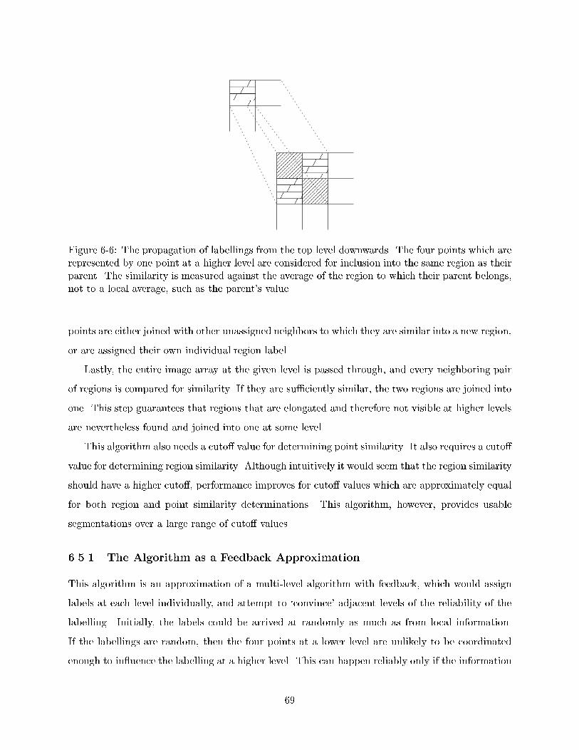
��������
����
���������������
���������������
������������
����
���
�������������������
������������
�������������������������
�������������������������
������
������
������������
������������
Figure 6-6: The propagation of labellings from the top level downwards. The four points which arerepresented by one point at a higher level are considered for inclusion into the same region as theirparent. The similarity is measured against the average of the region to which their parent belongs,not to a local average, such as the parent's value.
points are either joined with other unassigned neighbors to which they are similar into a new region,
or are assigned their own individual region label.
Lastly, the entire image array at the given level is passed through, and every neighboring pair
of regions is compared for similarity. If they are su�ciently similar, the two regions are joined into
one. This step guarantees that regions that are elongated and therefore not visible at higher levels
are nevertheless found and joined into one at some level.
This algorithm also needs a cuto� value for determining point similarity. It also requires a cuto�
value for determining region similarity. Although intuitively it would seem that the region similarity
should have a higher cuto�, performance improves for cuto� values which are approximately equal
for both region and point similarity determinations. This algorithm, however, provides usable
segmentations over a large range of cuto� values.
6.5.1 The Algorithm as a Feedback Approximation
This algorithm is an approximation of a multi-level algorithm with feedback, which would assign
labels at each level individually, and attempt to `convince' adjacent levels of the reliability of the
labelling. Initially, the labels could be arrived at randomly as much as from local information.
If the labellings are random, then the four points at a lower level are unlikely to be coordinated
enough to in uence the labelling at a higher level. This can happen reliably only if the information
69

Figure 6-7: The algorithm applied to the same image previously segmented with the Grow algo-rithms. The segmentations shown use cuto�s of 0.94, for the one next to the original image, 0.90,for the one below, and 0.80 for the third segmentation. The segmentation using a cuto� of 0.90 isthe segmentation which the Imagina system defaults to upon loading this image. The color labelsdisplayed are simply color markers used to visually denote the twenty most populous regions whichare segmented by the algorithm, and have no intrinsic meanings.
70

at both levels support the labelling. Thus, the information which is acquired locally is combined
with information which propagates from other levels.
6.5.2 Extensions
The algorithm could be improved by applying statistical information to the combination of means.
This can be done in two ways, either by considering the statistical reliability of the point values at
high levels of the Color Mapping, and which therefore are averages over large regions of the image
being segmented, or by considering the statistical reliability of the mean of a given region which
has been created and whose mean may represent only a few or many points.
In the former case, the pixel similarity required for joining points into a region would be higher
at a higher level of the Color Mapping than at a lower level. In the latter case, the pixel similarity
required for joining points into a region would be very low for regions containing only a few points.
However, as the regions would grow beyond a handful of points, the cuto� similarity would in-
crease. The di�culty with this approach is that some points may be included into a region without
belonging into the region after the range of inclusion becomes limited.
71

Chapter 7
Boundary Edge Extraction
There is a boundary to men's passions when they act from feelings; but none when
they are under the in uence of imagination.
Edmund Burke
After an image has been segmented, it consists of a set of one or more regions. Each region is
fully connected and contains pixels which are similar by some metric. The goal thus becomes to
come up with a description for the shape of that region. Di�erent shape descriptors are possible,
all of which operate on a set of edges describing the boundary of a region. This chapter describes
how these boundary edges can be extracted. The geometric descriptors that build upon these edges
will be the topic of the next chapter.
The edge extraction methods developed here assume an input region which is fully connected.
Moreover, its robustness relies on the input region being full. If holes are present, they can be �lled
as a preprocessing step to edge extraction. The goal of the edge extraction step is to construct
a connected set of edges that describes the boundary. This edge description can then be used to
compare region boundaries by di�erent methods, as described in chapter 8.
The purpose of edge extraction is to take the set of unordered points that form a region,
and construct a more meaningful representation that describes the region. From a pixel-based
representation, we would like to go to an edge-based representation. It is easier to compute with
72

edges, since they compress the information contained within the set of input pixels to a more
manageable form.
Edges are certainly only an approximation to the set of raw pixels. However, such a loss of detail
is inevitable when a processing step abstracts away from the raw image data. When constructing
the edge representation we introduce a bias to the information contained in the raw pixels due to
our choice of a particular algorithm to �nd the edges. However, �nding the edges distances us from
the raw pixel information and brings us closer to an abstract representation of an object.
7.1 Prior work
The edge extraction is a geometric processing step. Its purpose is to take a set of pixels, and turn
them into a more meaningful edge representation. Previous work comes from the computational
geometry community.
7.1.1 The Crust Algorithm
In computational geometry, a solution to a harder and more general problem has recently been
proposed. Amenta, Bern and Kamvysselis [1] published an algorithm that �nds the shape of an
object in three dimensions from sample points in its boundary. The algorithm is based on the
Voronoi diagram of a shape to �nd an approximation of the medial axis of the shape (see �gure
7-1). Based on that medial axis, the algorithm connects neighboring points that do not cross the
medial axis, the exterior of the object, its \crust". This algorithm is simple, fast and robust, and it
reconstructs a provably correct linear approximation of a shape that meets the sampling criterion.
Moreover, it only needs a set of unordered points to work upon.
To use the Crust algorithm, however, a preprocessing step is required on the points of the image
region in question, that �nds all the points on the boundary of the shape. The next section presents
an algorithm for �nding those points on the boundary. Section 7.3 goes a step further by using the
extra knowledge that we have of where the inside of the region is, and reconstructs the boundary
edges directly, without use of the Crust algorithm.
73

Figure 7-1: Two-dimensional Crust Algorithm. Left: The medial axis (in red) of a �gure is theset of all centers of circles inscibed in the �gure and touching its boundary in at least two points.Middle: The Voronoi centers (red points) approximate the medial axis. Right: Joining the nearestneighbors without crossing the medial axis gives an approximation to the shape.
7.2 Pixel-Based Boundary Extraction
Several straightforward approaches exist which allow the determination of the boundary of a region
after it has been segmented from the image. These are all based on processing the region on a
pixel-by-pixel level. Although these methods are easy to implement, they run into di�culties with
noise and special cases.
The simplest way to �nd the boundary of a region is to pass a window of 3 by 3 pixels over
the image, and label any center of the window as part of the boundary if the center is part of the
region and any other pixel in the current window is not part of the region. The resulting set of
pixels can then be sorted and connected, or walked over in a method which can detect loops.
Another approach to this problem is to circle the boundary of the region starting from a point
which is known to be on the boundary. Such a point can be found based on the center of mass of
the region. Given that the region is fully connected, that is, every pixel is reachable from every
other pixel within the region by passing through only region pixels, some pixel must have the same
x or y coordinate as the center of mass. Checking all y or x values along either of these coordinate
values, respectively, will yield a pixel location.
This starting position can be picked to be either on a left or a right edge of the region, by either
starting from the left or the right of the center of mass location. The direction of movement is
always forward with the region on the right; thus, starting on a left edge the direction of movement
74

A
B
C
D
Figure 7-2: The local pixel-based boundary growing algorithm. Pixels within the region are shaded,while pixels outside of the region are not. The current position is at B, and the current direction isshown by the arrow. C is the �rst position considered for the next step, and D is the next positionto which the algorithm will step to.
is upward, and on the right edge it is downwards. Based on the starting position and direction, the
current position is iteratively updated by stepping one pixel into the current direction.
Before stepping forward, however, the current direction has to be updated. It is tentatively
turned leftward by 45 degrees. The positions around the current pixels are then iteratively at-
tempted, going in order in a clockwise fashion around the pixel. This step is shown in Figure 7-2.
The position is then updated again, with the direction of this pixel from the current location. The
previous position is always the position in the opposite direction of the current direction. The next
position is always a pixel within the region whose boundary is being determined. The direction at
the end of a step is always in the direction of the next pixel to be considered.
In most cases, this method will succeed in describing the region boundary. This method, how-
ever, has several downfalls. Noise a�ects the boundary which is returned greatly. Single-pixel
connections between parts of a region also cause problems, requiring constant back-stepping and a
renewed attempt at edgewalking from a previously saved position. Although the base implementa-
tion is trivial, a fully correct implementation can become very complex.
The single advantage of this approach is that it provides a complete description of a region
boundary. From the list of pixels, any desired boundary description can be de�ned, because none
of the information, or noise, has been removed.
75

7.3 Window-Based Boundary Extraction
The fact that the shape is �lled to go a step further than the previous boundary walker, and
construct a new edge extraction algorithm. This algorithm considers a larger neighborhood of
points at each iteration, and guesses a boundary edge for each such window of computation.
Increasing the window size improves the reliability of the algorithm, as well as its robustness
against noise. Moreover, instead of points on the boundary, this algorithm constructs directly
boundary edges, so no postprocessing step is necessary.
At each step, the center of mass is computed for the `inside' and `outside' points within a window
of pixels. This information is then used to deduce the outer edge of the region being segmented,
as well as the direction of this edge. Edges are then combined into a perimeter, which is then
smoothed to remove multiple edges which are neighbors and nearly parallel.
Although the construction of the algorithm is serial, it can be easily parallelized by placing
the processing window as a �lter over every location of the image, and getting boundary edge
aproximations for each of window. Multiple scales can be run in parallel, and the di�erent layers
can then converge into a single multiscale boundary determination. The edge smoothing step, being
an approximation of the weighted interaction of multiple levels of detail, would not be required in
this case.
7.3.1 Algorithm Overview
The window-based boundary extraction algorithm �nds tangents to the extracted region at di�er-
ent points around it, and then constructs a piece-wise linear description of it. The tangents are
calculated on a window which contains at least one point of the region. Making the computation
window size larger results in a less precise but more robust edge description. A smaller window size
will pick out more detail, but will sometimes over�t a shape, by describing the noise which results
from the imperfections of the color segmentation phase.
The more tangents that are taken on the boundary, the more correct the description can be.
However, computation will be wasted for possibly similar nearby tangents and redundant infor-
mation. Similarly, a description can include hundreds of edges, or simply a few dozens. Nearby
small edges can be combined into larger ones if their slopes are similar. Again, the tradeo� exists
between the precision of many but almost identical edges, and fewer larger but less precise edges
in terms of the noise robustness and processing time cost.
76

7.3.2 Serialized vs. Parallel Algorithm
The algorithm described is implemented as a serial algorithm, for simplicity and e�ciency on a
single-processor machine. The parallel algorithm requires much more computation overall, but
drastically reduces the computation required of any single processor. In the parallel version, every
processor is responsible for �nding a single tangent at a single location for a single window size.
In the serial algorithm, one tangent is found at a time, for a particular location and a particular
window size. To optimize the algorithm the direction and position computed for one tangent are
used to determine a good placement for the next window of computation. In a parallel version of
the algorithm, several window sizes would be applied independently at each image location. We
will not describe further the parallel algorithm. Instead, we will concentrate instead on the actual
implementation of its serialized counterpart.
7.3.3 Computation within a Window
Within each window we calculate the center of mass of the points belonging to the region, and the
center of mass of the points outside of the region. The perpendicular bisector of the segment joining
the two centers gives the direction of the edge. The relative sizes of the 'inner' and 'outer' regions
within the window give the position of the edge. Moreover since we know which center represents
the inside and which the outside of the region, we can construct directed edges for the boundary.
Choosing the window size
The window size is an important parameter for the algorithm to work. If a shape is large and free
of holes, then a large window size works most of the time. The few times a large window size is
inadequate is when the region has sharp corners, where a smaller window size is needed. A smaller
window size can be chosen for objects that contain narrow parts, such as the picture of a hand
with �ngers spread. When the region is thinner than the window size, the window size should be
reduced.
Increasing the window size
When the center of processing is either too far in the region and there are no outside pixels within
the window size, or when it is too far outside the picture and there are no region pixels within the
window size, then there is no information on how to proceed. The tangent cannot be calculated
77

Pi
Cout
Cin
Edge Added
Pi
Cout
Cin
Step
Siz
ePi
Cout
Cin
WindowSize
Pi+1
Pi
Cout
Cin
Window Size
Ti
Ti
Ti
Ti+1
1. Find Centers of Mass 2. Weighted Average is Tangency Point
3. Edge of length 2*stepSizecentered at Ti and
perpendicular to CinCout
4. Set Pi+1 at the end of the edge as the new window center
Figure 7-3: The Edges Boundary Extraction Algorithm �nds an approximation to an edge withina window of computation. It calculates the center of mass Cin of the points belonging in the regionand the center of mass Cout of the poitns belonging to the outside of the region within the windowof computation. It uses the number of points belonging to the inside and the outside to calculate aweighted average of Cin and Cout, that will serve as an approximation to the tangent point to theregion's boundary. A tangent direction is calculated to be parallel to the perpendicular bisector ofCinCout. Finally, a new window center is calculated by moving along the tangent.
78

No inside points No outside points
Figure 7-4: Increasing the window size: When there is not enough information within a window forcalculating an edge, the window size is increased until enough information is present. This �gureexhibits two cases where this situation arises. Where there are no inside points or there are nooutside points, the window doesn't have enough information to place an edge, since only one centerof mass can be calculated. A more subtle case arises when the two centers of mass coincide, notshown in the �gure.
79

and the progression is stuck. In that case, a simple solution is to increase the window size until
both inside and outside points are included with the window of computation. Once the boundary
is found again, the window size can be restored at the next step. Another case when there is not
enough information to determine an edge is when the inside and outside centers coincide. In that
Placing the window of processing
As described above, in a parallel algorithm where large numbers of parallel resources are available,
a window can be placed at every point in the image and obtain a lot of tangents that can be joined
to construct an object.
On a single processor, we should limit the number of such computations. Therefore, a window
is placed only at points on the contour of the region, where part of the window contains pixels
inside the region, and part of the window contains outside points.
The �rst window is placed by simply following a line from the outmost point of the image
towards the center of mass of the region. When a pixel belonging to the region is encountered, the
center of the window is placed.
Once a tangent has been found within the current window, subsequent windows are centered by
moving along the direction speci�ed by the tangent. The process is then repeated until the edges
have gone full circle returning to the initial starting point, or until a certain maximum number of
iterations is reached.
Step Size vs. Window Size
To determine how far to move on the direction of the tangent before placing the center of a new
window of processing, we use one more parameter, the step size, which determines the absolute
distance between two consecutive window centers.
The two notions of window size and step size are related but not the same. The window size
determines how many pixels are going to be used for the computation of a particular tangent. The
step size determines how many tangents are going to be computed. Together, they determine how
much computation will be spent on extracting the edges of a particular region.
Several groupings of window and step sizes can be considered:
� With a large window size and a small step size, many certain steps are taken in going around
the region. This method is going to ignore noise, as well as detail on the shape boundary.
80

Edge Added
WindowSize
Pi+1
Pi
Cout
Cin
Step
Size
Figure 7-5: The di�erence between window size and step size. The window size determines howmuch computation is performed at every iteration. The step size determines the frequency ofsampling around the boundary.
81

This is the most expensive computation.
� With a small window size and a small step size, the algorithm will pick out the most details,
but also be prone to error.
� With a small window size and a large step size, the algorithm will be very likely to overshoot
because of a small deviation in the boundary. It will be misled by little twitches in the region
boundary which could be due to noise.
� With a large window size and a large step size, the algorithm will �nd few edges, but each of
them will have enough information to make a noise-tolerant decision on what the boundary
position and orientation are. By ignoring noise though, this method also ignores possibly
useful detail.
There is no golden rule on how to make these value choices. Most certainly the same region
will need di�erent window sizes at di�erent parts of its boundary. A simple way to achieve this
e�ect is to have a default window size corresponding to the desired level of detail, and changing
that window size as the conditions around the region change. When only inside or only outside
points are found within the window, the window size should be increased. When either the inside
points or the outside points fail to form a connected subregion within the window, the window size
should be reduced after moving the center closer to the boundary.
7.3.4 Determining a tangent
Once the window has been placed and the window size has been chosen, we can compute a tangent
for the region boundary at that part of the image. The direction of the tangent, along with the
position of the region boundary, together determine a straight line where an edge will lie. Using
the step size we can set a length on that straight line, and thus determine an edge, whose midpoint
is the point we found on the boundary.
Finding a direction for the tangent
Within the given window of computation, we would like to determine a single edge. To do so, we
need a direction and a midpoint. The optimal direction is tangential to the region. This tangent is
perpendicular to a vector that is easy to approximate.
82

WindowSize andEdge Re-construction
Figure 7-6: Decreasing the level of detail. A higher window size causes a greater tolerance tonoise, and provides a rough estimate of the shape. A smaller window size allows more attention todetail, but also generates lengthier representations that might be harder to work with and mightbe over�tting noise from the segmentation.
83

We can compute the center of mass Cin of the points inside the region, and the center of mass
Cout of the points outside the region. The vector�!
CinCout is a good approximation for the normal
to the boundary within the window. The direction of the tangent is simply perpendicular to that
vector.
Finding a point on the boundary
Now we have to �nd a point on the approximated boundary between the inside and outside points.
One way of �nding such a point would be to move on the line that connects Cout to Cin until a
point in the region is found. This method is inadequate because it will trust a single pixel of the
region which could be the result of noise. More importantly though, it is inadequate because it
goes against the spirit of approximation that the window method was developed in. We are really
not looking for a perfect tangent to the region. We are looking instead for an edge representative
of the region boundary in the particular window of computation. Therefore, instead of relying on
individual pixels, we rely again on the two representative points that we found.
Since Cout is a representative of the outside of the image, and Cin is a representative of the
inside of the image, the boundary should lie somewhere between the two. We could choose the
middle of the segment joining the two centers, but we can do a little better than that. We can
weight this average of Cin and Cout by the number of pixels belonging to each region. Thus, we
can a formula for Ti, an approximation for the boundary point.
Ti = (Cini�Numpointsin + Couti �Numpointsout)=(Numpointsin +Numpointsout) (7.1)
Adding an Edge to the set of edges
Once a direction and a boundary point is set, we simply add an edge to the set of edges, centered at
the boundary point with a length of 2 � stepsize. Since the next center will be stepsize away, such
a length is a good choice for a representative edge. The length of the edge is not that important
since an edge's endpoints will later be extended or brought closer until the intersections with the
two neighboring edges.
84

Figure 7-7: The complete boundary at the highest level of detail. A moderate window size and asmall step size pick out the most detail from the shape
7.3.5 Post-processing on the Edges Found
Once those edges have been added, they undergo two stages of postprocessing before they can be
passed on to the next stage that will use them to construct shape descriptors. This post-processing
gets rid of the useless tips of intersecting edges, and compresses the representation by combining
small consecutive edges that have similar slopes into larger edges.
Intersecting the Edges
The edge intersection is easy, since by applying a sequential algorithm the edges are already ordered
by circling around the region. In the parallel form of the algorithm one would have to determine
which edge to intersect with which other edge. In the serial case however, the choice is obvious.
We simply set the endpoint of edge i to the intersection of edges i and i+1, and the starting point
of edge i+ 1 to that same intersection.
A complication arises when the two edges are nearly parallel. In that case the intersection falls
too far out, and setting the endpoints to meet at in�nity might not be the right decision to make.
Therefore, we constrain the intersection of two edges to fall within the bounding box surrounding
85

the two edges. If the intersection falls outside that bounding box, then the midpoints of the two
endpoints to be modi�ed is chosen as the new value for both endpoints. After this step, the region
is surrounded by a piecewise linear continuous set of edges.
Joining similar edges
Once the edge endpoints are made continuous, that is once the end of one is the beginning of the
next, a compression step can be carried out. One can make the edge representation of a region
more compact by replacing small consecutive edges by larger ones if the small edges are nearly
parallel.
This step is not a fundamental part of the algorithm, but can reduce the number of edges in
the representation by a large factor. In our tests, tenfold reductions of the number of edges is not
uncommon. The resulting loss in detail is negligible when compared to the much smaller number
of edges.
One more parameter, cosineCuto�, speci�es when two consecutive edges should be joined. The
joining is simply based on the angle between the two edges, and never on the length of either edge.
If the cosine of the angle between the two consecutive edges is larger than cosineCuto�, the two
edges are joined.
When two edges are joined, the begin point of the �rst and the end point of the second are kept
unmodi�ed. A larger edge with those endpoints is created and replaces the previous two. Begin and
end point can be determined simply since edges are oriented, circling the region counter-clockwise.
A simple version of the algorithm can be made serial, going around the region, and combining
every similar edge with a progressively growing �rst edge. The disadvantages of this method is that
�rst, it can't be implemented on a multiprocessors, and second, its result will depend on the order
in which we circle around the region. Moreover, this version will have a tendency to growing some
edges more than others, resulting in an unbalanced description.
Instead, we implemented an algorithm that is more easily ported on a multiprocessor. It
compares neighboring edges two by two and combines similar ones into larger edges. It then
compares the combinations two by two, and again combines similar ones. This hierarchical method
has the advantage of being independent of starting point or direction of rotation. It has the
advantage of being easily implementable on a multiprocessor. Finally, it has the advantage of
generating progressively less precise descriptions of the object, that can be used for matching at
86

di�erent levels of detail.
Independent of the algorithm that implements it, the step of combining similar edges into larger
ones has the advantage of making the �nal description less dependent on the step size. Therefore,
a smaller step size will pick out more detail if it's available, but will represent large straight sides
compactly, by replacing them with a single edge. The step size can therefore be made smaller
without risking cumbersome descriptions and having to later match a very large number of edges.
7.3.6 Improvements and Extensions
Several extensions are possible to this algorithm. The �rst two are elaborations on the current
processing methodology. The last two provide a di�erent way of thinking about the algorithm and
change its function in general.
Decreasing the window size
The major aw of the current algorithm is that it doesn't have a way of detecting when the window
size is too big. A simple way to get around this problem is to always start with a small window
size, and augment it as needed. However, for completeness we could extend the algorithm to detect
when the window size is inappropriately big for the shape to be extracted. This situation arises
when the window contains more than one surfaces of the region. This is the case in crevaces in the
�gure, where the full detail of a crevace will rarily be explored. This situation arises also in thin
objects, that cut diagonally through the window size. In both of the above cases, the averaging
will not yield an appropriate measure of the boundary edge position. One way of dealing with this
problem is to draw a line between the outside center and the inside center, and obseve how many
times the line crosses a boundary of the region. If this number is higher than one, then clearly
the shape is a stripe through the window, and the window size must be reduced. The new smaller
window must be centered closer to the surface otherwise it might not include any region pixels, in
which case its size would have to be increased once more. To move the center closer to the region,
one can simply follow the line from the outside center to the inside center and set the new center
where the line intersects the region.
87

Changing the Shape of the Window
Another simple �x is to change the window size to be more rounded than the square currently
used. A square is certainly easy to deal with, but it doesn't give equal importance to all points
at the same distance from the center of computation. It will consider points along the diagonal
that are further away than points along the vertical and horizontal axis. Along with considering
a circle as shape of the window of computation, we can furthermore change the absolute cuto� of
the window size for considering pixels in the computation. Instead we could assign an importance
metric to each pixel, depending on its distance from the center of computation, and calculate a
weighted average instead of an unweighted one on the pixels of the fuzzy region.
A novel similarity metric for region membership
Moreover, instead of having a discreet value that is either zero or one, one can assign a oating point
number that can take all values in between. The labels would thus be replaced with a computation
every time the pixel is accessed, that evaluates a similarity metric between the pixel being currently
processed, and the average of the region it belongs to. This similarity metric can be based solely
on color, texture, shadowing, or other criteria. It should return a value between 0 and 1 however,
where 1 means the pixel belongs without doubt to the region, 0 means the pixels de�nitely doesn't
belong to the region, with all possible values of certainty between the two.
When the centers of mass of the window are being computed, certain pixels will only contribute
partly to the calculation, instead of either belonging or not belonging to the region, thus achieving
a greater precision in the calculation. This extension in fact would make the region extraction
step obsolete. The edge extraction algorithm could be directly applied to the raw image pixels. To
determine the average color of a region however, a �lter must be applied to the image to �nd patches
of similar colors. This would be a much simpler form of the current segmentation mechanism
described in chapter 6. However, since the segmentation functionality is already provided both
globally and locally with the grow algorithms, no such extension of the algorithm was implemented.
Multiple Levels
Finally, instead of inheriting the window size from the system surrounding it, the edges extraction
algorithm could operate itself at multiple levels. This extension is closer to the biological approach,
where parallel computation is used to distribute load from a single serial processor. When using
88

multiple levels, higher levels, which have larger window sizes, can reinforce the lower levels, which
have smaller window sizes. By using this combined information, edge smoothing and even region
extraction can be performed in parallel across an image. This process is also fully parallelizable.
This approach then becomes similar to �ltering, which is described in chapter 5.
7.4 Conclusions
This chapter presented a new algorithm for extracting the edges from a region. The algorithm
assumes we have labelled the inside and the outside of the region whose boundary is sought. If
these labels are not present, then a pixel-based metric such as color similarity must be used to
determine if a pixel belongs to the region or not.
The algorithm presented uses a window-based approach to edge extraction which is both simple
to implement, computationally cheap, and robust. Moreover, instead of complex mathematical
operations, it uses simple averaging and estimation techniques which are feasible in a biological
system. Finally, it can be implemented as a distributed algorithm.
The shortcoming of this algorithm is that it requires input parameters such as the window size,
step size and the cosine cuto� for combining edges, that can cause changes in the output. These
parameters could be combined within a single parameter determining the level of detail at which
the edges should be extracted.
89

Chapter 8
Shape Representation and Region
Matching
Thou com'st in such a questionable shape, That I will speak to thee.
William Shakespeare, Hamlet
The previous chapter described a way to extract boundary edges from an image region. This
set of edges is the basis for the various shape descriptors we use. From the same set of boundary
edges, di�erent representations are constructed. Each emphasizes a di�erent criterion one can use
in comparing two shapes. Those criteria of comparison are area overlap, relative edge positions,
orientation of edge normals, and the number and size of protrusions. These four ways of describing
shape will be the topic of this chapter.
8.1 Literature on Shape Descriptors
Shape description is a fundamental problem faced in image retrieval, as well as vision and graphics.
From each of these �elds, we have chosen a representative example that in uenced us in our
approach to shape description.
90

8.1.1 Image Retrieval and Shape Description
Previous work on descriptors for image retrieval includes mostly global processing of pixel positions
and wavelets. Shape is rarely discussed. In fact, shape is mostly unused in image retrieval systems.
The exception is probably BlobWorld [5], in which generalized ellipses are used to represent
shape. This method can be though of as a series of ellipses superimposed adding or subtracting
detail to the shape. The �rst ellipse gives a rough estimate of the shape, mostly of its orientation.
Subsequent ellipses add more detail.
Generalized ellipses are a very successful shape descriptor. They provide noise tolerance when
few ellipses are used. Moreover, they provide incremental addition of detail, which can make
comparison more e�cient, by pruning bad matches early in the search tree. We hope to integrate
in the future an algorithm based on generalized ellipses as one of our shape descriptors in Imagina.
At this stage, we mostly experimented with four new shape descriptors.
8.1.2 Vision and Shape Description
Shape description has been largely discussed in the computer vision literature. We won't review
here the various approaches here. We are mostly interested in representations that provide multiple
resolutions. The most noteworthy example of such a representation is [38], that uses hyperbolic
evolution of shape to create a hierarchy of shape features. The shape simpli�cation that occurs is
analogous to viewing an object from various distances. A follow-up paper [37] uses this idea for
shape matching, and results in a language for describing shape. The base of the description closely
matches the medial axis of a shape, the locus of all centers of spheres inscribed in a �gure that
touch exactly three points in the boundary.
8.1.3 Graphics and Shape Description
The computer graphics problem that inspired us the most for shape representation is that of
morphing. Morphing is the procedure of transforming one shape into another in a continuous
progression. If we have a way of assigning a cost to a particular morph between a source shape and
a target shape, then we can use that metric to evaluate shape similarity. The best match between
two shapes will be the one which has the least morphing cost.
The problem with most current morphing techniques is that the task of �nding edges in the
picture, and matching source and target shapes is left to the user. This is a reasonable thing to do
91

if the goal of the system is to create a good looking morph. Our goal however is to distance the
user from such low-level decision on where edges arise and how they are transformed. We already
have a way of extracting the edges. We now need a way to �nd how well the edges of one object
match the edge of another.
Manolis Kamvysselis [18] proposed a novel technique for �nding edge correspondences in mor-
phing convex shapes. This technique �rst maps the two shapes into their Extended Circular Images
(ECI), and then does the morphing in the ECI space. A one-to-one mapping exists between convex
shapes and their ECI representations. Hence, every intermediate ECI obtained can be transformed
into the corresponding shape. The ECI space seems like a good for morphing where such a metric
can be found, and the results obtained in morphing shapes in the ECI space are promising.
The ECI representation of a shape maps every edge to a weight on the unit circle (see �gure
8-1). The angle of the edge normal determines the position where the weight will be placed on the
unit circle, and the length of the edge determines the weight that will be placed there. Morphing
can then be done by simply transforming the weights of the source to the weights of the target.
In ECImorph, the transformation is simply an all-to-all mapping of weights based on an inverse
exponential cost function taking into account both angle di�erence and weight di�erence.
What matters more to us is the overall cost of the morphing transformation, rather than the
cost breakdown among individual edges. We are interested not in the way individual edges map
to each other, or the particular matching algorithm found, but instead in �nding a metric for an
overall cost of transforming one shape into another. Such a morphing metric is the best candidate
for a shape matching metric.
8.2 Shape Descriptors Used in Imagina
Since each representation is designed for comparison, the representation and the corresponding
comparison method are best described jointly. This section will describe in detail each shape-based
representation, its normalization metrics, and the comparison algorithm.
The di�erent shape-based representations built on top of the boundary edges are:
� Volume based representation: Two regions are similar if they have a large number of
common points when they are superimposed and adequately scaled.
� Segment based representation: Once aligned and scaled, two regions are similar if the
92

Figure 8-1: The Extended Circular Image (ECI) of a Convex Shape is constructed by mappingedges to weights on the unit circle. The left frame displays the original polygon along with thenormals to the edges. The normal lengths are proportional to the lengths of the edges. The middleframe displays the weights on the unit sphere. The third frame displays a graph of the ECI weightsobtained by unrolling the unit circle onto a at axis.
segments making up the boundary of one are nearby those making up the boundary of the
other, and vice-versa.
� Angle based representation: Once perimeters have been adjusted and the regions ro-
tated, two regions are similar if for every angle between 0 and 2�, the edges with normals
facing towards that angle have similar sums of lengths.
� Protrusion based representation: Two regions are similar if they have similar protru-
sions located at equivalent points around the convex inner perimeter of the shape.
Each representation has di�erent applications and strong points. This chapter will describe the
representations developed, the scaling and alignment metrics used, and the matching algorithms
developed.
In the remainder of this section, we present a few simple region descriptors, based on di�erent
features of geometric shape. We use the boundary edges extracted at the previous processing step
as the basis for these descriptions.
93

8.3 Volume Based Representation and Comparison
The simplest representation is simply that of the set of points that belong to the inside of region.
Comparison is done by superimposing two scaled and aligned regions, and comparing the number
of pixels in common to the total number of pixels.
8.3.1 Approximating the Inside Points
From the set of edges, one can �nd all the points inside the region by using common computer
graphics techniques. However, such techniques are expensive, and moreover, we already have the
pixel information from which the edges were constructed in the �rst place.
We need however to approximate the set of inside points to make the expensive computation of
comparing every pixel in a region more feasible in an interactive query environment. The way we
do that is by undersampling the picture. Instead of considering every single pixel, one can consider
one pixel out of 4, one out of 16, and so on, with similar results. In fact our assumption that the
shapes are �lled gives us an easy argument that such a measure can be adequate without a need to
sample every point. Our preprocessing step of �lling the shapes guarantees that this assumption
holds.
8.3.2 Scaling and Alignment
The shapes are scaled so that they have the same areas. Since the area overlap is used as the
metric of comparison, unequal surface areas could bias the results towards thinking that a small
area entirely included in a larger one matches perfectly with it. Similarly, a large area would always
have a relatively small area of overlap with a smaller region entirely included within it. These two
biases do not balance out, since each of them saturates the results in the entirety of the small
region, in the case of complete containment. Scaling the two regions so that they have the same
area gives the desired size invariance of the comparison.
The shapes to be compared must also be aligned for area of overlap to be a signi�cant metric.
The two regions are aligned so that their centers of gravity coincide. An alternative would be to
align the bounding boxes of the two regions. However, the bounding box is a metric that depends
only on the extremities of the region, rather than the entire inside of the region. Therefore, if a
silhouette of a person with both hands extended to the right is matched with that of a person with
only one hand extended, the result is going to be very dissimilar. If however the center of mass is
94

used as an alignment position, these two shapes will be more rightfully judged more similar.
The shapes are not stretched, nor are they rotated. We believe that the aspect ratio of a shape
is an important metric that should not be lost in scaling. Also, the angle based representation takes
care of rotating the two shapes, so we did not want to take care of that concern here, especially
since it would make a straightforward computation much more expensive.
8.3.3 Similarity Metric
Similarity can be measured in two ways. One way is to simply ignore the original color that was
used in separating each shape, and return a value of 1 for every pixel in common, and a value of 0
for every pixel that is not in common. The sum is divided by the total number of pixels, and we
have a similarity metric between 0 and 1. In this case, we are simply comparing areas of the two
shapes.
Another way of comparison goes a step further by considering more degrees of membership to
the region than 'inside' and 'outside'. For a region, the color similarity of every pixel to the average
of the entire region in which it belongs can be used to determine a membership value that can be
anywhere between 0 and 1, rather than just 0 or 1. The use of color here is di�erent than the one
in the color-based comparison. Color is not compared between the two regions. Color is instead
used within each region to determine the degree of membership of a particular pixel to the overall
regions that it represents.
If this similarity value between 0 and 1 is considered to be the thickness of the shape de�ned
by each region, then the overlap between the two regions becomes the volume that the two aligned
shapes have in common. It is therefore not a planar comparison of surface areas that this algorithm
performs, but instead a comparison of volumes in two and a half dimensions, where the thickness
is the similarity of the shapes, between 0 and 1.
8.3.4 Results
Figure 8-2 shows an example of a volume-based comparison on two images of the St. Louis Arch. If
one considers the color histograms of the two images, they will appear very dissimilar, as is shown
in �gure 8-3. Having a shape-based comparison allows an robustness to lighting conditions when
searching for a particular image.
Many current image retrieval systems that rely heavily upon color information will be less likely
95

CA
E FD
B
Figure 8-2: The Volume-Based Comparison. A shows the original image, along with the center ofmass of the region's pixels and the bounding box around the selected region. B shows the pixelsbelonging to the region. C shows in blue the pixels in B that do not also belong to E and in redthe pixels that B and E have in common . Similarly, F shows in blue the pixels that belong to Ebut not in B, and in red the pixels belonging to both B and E. The similarity metric returned is thenumber of pixels in common (red) over the total number of pixels (blue and red). The similaritymetric returned for this match is 0:87.
96

Histogram of Image DHistogram of Image A
Figure 8-3: The color histograms of Images A and D have a similarity of only 0.19. The horizontalaxis represents di�erent color buckets, and the four vertical axes represent from top to bottomnumber of points in a bucket, standard devitation of Hue, standard devitation of Saturation, stan-dard devitation of Value, in the HSV color space. Picture D spans the entire blue color bucket,while picture A contains primariliy one spike in a single tone of blue. Moreover, the shape of thedistribution of grey in the two images doesn't match.
to �nd the match between these two images. This is demonstrated in the results returned by the
Altavista Image Finder when picture A is used as the query to a similarity search. The best matches
returned are displayed in �gure C-3 in appendix C. The Virage engine for matching images does
not seem to give any importance to shape in this example.
In Imagina, the shape of the region under the two arches is a salient feature to match, since it's
large, uniform, and centered. It will be segmented as a single region, since the color under the arch
is uniform. Its shape will then be matched to the shape of the corresponding region in the target
picture, and a high similarity will be returned.
8.3.5 Shortcomings and Strong Points of a Volume Based Representation
This representation is best �t for matching regions that have roughly the same overall shape but
whose boundary details may diverge. The strong point of it is a tolerance to noise created by holes in
the image. Geometric representations will consider a shape with a hole as a topologically di�erent
object from the �lled shape. Similarly, representations based on edges will tend to give more
importance to high frequency changes in the region boundary, while a volume-based representation
97

will be unperturbated.
The main disadvantage of this method is that it breaks when the alignment between two shapes
is not adequate. This situation arises if the segmentation for one image assigns a larger portion of
the image to a region on one side, and segmentation for the other image assigned a larger portion of
the image on the other side. In that case , the two images will be misaligning, and the two shapes
won't match. This situation arises too often for thin shapes, since their overlap can be reduced
drastically with small misalignments.
An example where this representation breaks is the matching of Marylin to a drawing that will
be our criterion for the rest of the representations.
Figure 8-4: The Volume-Based Comparison breaks for �gures with many details. For example, onthe image on the right, even though the dress of Marilyn has the same overall shape, it is misaligneddue to noise in the segmentation, and this causes the area of the hands to be miscounted.
8.4 Segment-Based Representation
The segments-based representation comes as an aswer to the fact that the volume based repre-
sentation breaks for thin images. In the example of Marylin, when her hands are misaligned, the
match su�ers heavily. Finding a better alignment for the volume-based representation might be
98

an asnwer, but again, small di�erences in angle that do not matter to the user will count heavily
against a volume-based match.
Figure 8-5: The Segments-Based Comparison. On the left, every edge on the original image ismatched with its nearest edge in the query. Segments are drawn between the midpoints of thematched edges as a visual feedback. The sum of the lowest costs for every edge becomes the costof mapping database edges to query edges. On the right, each query edge is matched with the bestdatabase edge. Similarly the cost of mapping the query to the database is computed. Togetherthese two costs become the cost of transforming one shape to the other. The value obtained in thismatch is 0.94. Of course, this value alone is meaningless, since it will be normalized according tothe distribution of all segment based matches, when the matches from di�erent representations arecombined.
The metric of similarity in the segments-based representation takes into account the proximity
of the �gure's boundary edges. Proximity is calculated on an edge by edge basis. The metric used is
comparing two edges is based on coordinate proximity of the segments midpoints, angle similarity
between the two normals of the edges considered, and the length ratio between the edges. These
three metrics of every edge are combined in an overall cost of matching one edge with another. The
cost and the similarity are complementary of each other, and are both between 0 and 1. Their sum
is always 1.
The aspect ratio of the regions is preserved, but the regions are scaled and aligned with each
99

other. We believe aspect ratio is important in matching images, and the users have a good idea of
the relative dimensions of a shape they are looking for. Moreover, the aspect ratio is often invariant
between di�erent pictures, although the pictures can be found in all sizes and alignments within a
picture.
The two representations are scaled so that their bounding boxes have equal diagonals. The
bounding box is used since this representation is based on boundary edges, hence if the boundary
matches, the bounding boxes will be similar. The diagonal of the bounding boxes is used instead of
the area, because it gives a more uniform rate of change with changing dimensions of the bounding
box. That is, when one dimension becomes dominant, the diagonal does not vary geometrically,
while the surface area would.
Finally, the two regions ar aligned so that the centers of their bounding boxes coincide. This
metric is used instead of the center of mass which would not be meaningfull in a represenation
based on boundary edges rather than volume. Moreover, by aligning the centers of the bounding
boxes, this brings the edges closest to each other overall.
8.5 Angle Based Representation and the Extended Gaussian Im-
age
Based on the work of Kamvysselis [?] described in section ?? we construct an angle-based repre-
sentation for shapes that relies on the Extended Circular Image (ECI).
The di�erence from the original ECI representation lies in the creation of angle buckets that
contain more than one angle value. By choosing the number of buckets, one can determine how
precise the ECI representation will be made. This provides even at this representation level another
metric for noise tolerance or attention to detail. Our experience shows that 20 buckets are adequate
for matching most shapes. Fewer buckets give too coarse descriptions and more buckets tend to
separate almost similar shapes.
The Angle-Based representation creates a number of buckets that contain di�erent partitions
of the angle space and goes around the edges, consecutively adding to each bucket the length of
each edge belonging to the bucket.
Comparison is done at the bucket level, by simply measuring angle di�erences between nearby
buckets and length added within each bucket. Comparison between angleBuckets with di�erent
number of buckets is disallowed, but can easily be extended by reprojecting and recalculating the
100

Figure 8-6: The Angle-Based Comparison for Marilyn with only 8 buckets. The two representationsare rotated for achieving an optimal match.
101

angles that the corresponding buckets would give.
The debug information shows the buckets painted as edges with the corresponding length and
the middle angle of the bucket, centered at the center of the �gure.
The strong points of this representation is that it is rotation invariant, and tolerant to small
errors in angle, when the overall orientation and derivatives match. In that case it is similar to the
generalized ellipses described in [5].
8.6 Shape Descriptor based on Protrusions
From the congitive science community, we borrow the idea that protrusions is what humans base
their recognition upon. The shape of crevaces in the region boundary does not matter, but instead
the protrusions that bulge out of an image is what humans have learned to recognize.
Based on this assumption, we constructed a representation that uses mainly protrusions in
the matching. Protrusions are extracted from the edge-based representation of the boundary, by
considering adjacent edges two by two, and using the angle between them to label each edge as a
protrusion edge or an inner-perimeter edge.
Once the set of protrusions for each image has been extracted, the protrusions are matched in
order based on their position on the inner perimeter, the outer perimeter of each protrusion, the
length of the base, and the orientation of the protrusion's center of mass with respect to the base.
Scaling is done by aligning two separate but not independent metrics, the inner and the outer
parameters. The inner parameter is formed by the non-protrusion edges, along with the bases of
protrusions. The outer perimeter is the sum of the lengths of protrusion edges.
8.7 A metric for combining comparisons from individual meth-
ods
Instead of returning an absolute proximity metric, we return a relative one. That is, when two
di�erent represenations are used, say based on color and based on shape, we have to have some way
of comparing the outputs of the corresponding comparison funcions in the two di�erent domains.
In each domain, the comparison function returns a value between 0 and 1, where identical repre-
sentations that are 100% similar have a similarity value of 1 and dissimilar images have a similarity
value of 0. However, this scheme breaks down when say, every image in a particular representation
102
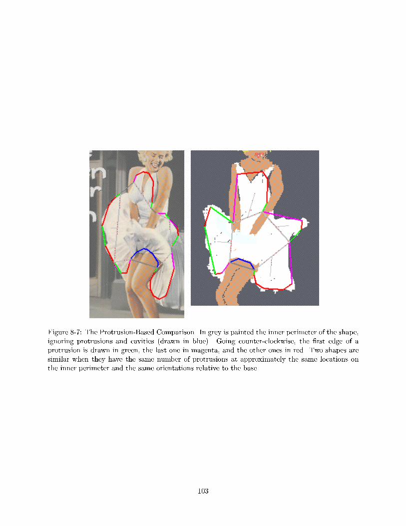
Figure 8-7: The Protrusion-Based Comparison. In grey is painted the inner perimeter of the shape,ignoring protrusions and cavities (drawn in blue). Going counter-clockwise, the �rst edge of aprotrusion is drawn in green, the last one in magenta, and the other ones in red. Two shapes aresimilar when they have the same number of protrusions at approximately the same locations onthe inner perimeter and the same orientations relative to the base.
103

has the same representation. Thus if a representation is broken it might advertise a similarity of 1
with every other image, and might bias the search to use that particular representation.
Therefore, we will use a relative metric based on these absolute similarity values. This metric
measures the similarity of the query to a particular image as compared to its dissimilarity to the
rest of the images. Therefore, for a particular representation, we will return as the proximity metric
of the best image the ratio between the similarity value of the best image and the average similarity
value.
8.8 Conclusion
This chapter presented a combination of di�erent approaches for describing shapes, each having
speci�c strong points and being tailored to speci�c applications. All of them have weak points,
but when one fails usually the others take over, thus providing a graceful degradation of the shape
description.
104

Chapter 9
Image Retrieval and Matching
Though we travel the world over to �nd the beautiful, we must carry it with us or we
�nd it not.
Ralph Waldo Emerson
Image retrieval and matching brings together the work of the previous chapters into the system
of Imagina. All of the methods of region matching which are used in Imagina have already been
presented. The next step is the combination of the representations into a uni�ed measure of match
between regions. Image matching based upon this, and a simple con�guration measure, is then
straightforward.
Once the similarity between regions can be measured, the similarity between images can be
computed. This measurement then allows for the comparison of similarity between a query and
the images stored in the database, yielding a content-based image retrieval system.
The problem of image retrieval is not as straightforward as this might imply. Image retrieval is
a hard problem because the problem itself is ill-de�ned. Given a query image and several database
images side by side, few people would be able to agree on which of the images provides the best
match. This, however, is exactly what an image retrieval system is expected to do.
105

9.1 Challenge of Classi�cation
Classi�cation, whether in terms of image segmentation or shape matching, is an ill-de�ned problem.
Without a bias for a category of solutions, a useful answer can never be achieved. How else can
the \right" answer be identi�ed? Although intuitively the \simplest" answer matching the desired
criteria is the right one, this is not always as straightforward as it seems from our evolutionarily
advanced vantagepoint. Computer systems, lacking such a concept, need a more stringent de�nition.
The following example illustrates this. The example is borrowed from [26, pages 21-22]. Take
a minute to look at the training set on the left, determine the classi�cation rule which is being
sampled, and consider possible test set item labellings.
Training Set Test Set
Attribute 1234
1 1 0 1 0 0 1 01 1 1 0 0 0 0 11 0 1 0 1 0 1 01 0 1 0 0 1 0 1
0 0 0 1 1 1 0 10 0 1 0 1 1 1 00 1 0 1 0 1 0 10 1 0 1 0 1 0 1
Category A A A A B B B B ? ? ? ? ? ? ? ?
Table 9.1: Pattern classi�cation task example.
In Table 9.1, several rules may be valid. For example, the label `A' could represent the NXOR of
attributes 3 and 4, while the label `B' could represent the XOR of attributes 3 and 4. Alternately,
A could be the AND of attributes 1 and 2 ORed with the NXOR of attributes 2 and 3. A variety of
other solutions come to mind. The basic di�culty lies in that, since the entire space of solutions can
never be seen in its whole as examples, the classi�cation rules must make assumptions about the
space they are operating in. Otherwise, the rules would never be able to classify unseen examples.
This problem only becomes more di�cult when noise is introduced into the system. Then, errors
would occur even if the ideal classi�er were to be known. In case this problem seems too simple,
consider this: the solution which seems simplest based on the number of attribute combinations
required, the XOR of attributes 3 and 4, yields a homogenous pattern labelling for the test set.
Given that the training set had two equally-represented sets, would it not make sense that a random
test set would contain roughly equal numbers of examples from each category? The correct choice
of classi�cation rule is, after all, dependent on the task that is being solved.
106

9.2 Combining the Representations
In performing the image retrieval version of classi�cation, unrelated measures provided by di�erent
representations need to be combined. This is done through the application of the concept of how
to combine unrelated measures presented in section 3.6. This idea was applied in Imagina both for
the region and the image search implementations.
For region searching, the similarity measures computed by the comparison of the di�erent
representations which are abstracted from each region must be combined. Based on this idea, the
measures are �rst normalized before being summed into an overall match score. In order to be able
to do this, the distribution of every measure has to be normalized. Therefore, assuming a normal
distribution for each similarity measure computation, the mean and the standard deviations of each
distribution must be computed.
In a large database the distributions can be approximated through random sampling. In a small
database, however, the distribution can best be approximated by looking at all of the sample points
available. Therefore, regions are matched sequentially against all otehr regions in the database.
The distribution of results of one match may not be a good predictor for the distribution of
results for another match. Therefore, the distributions of the similarity values returned by each
representation are recomputed each time a region gets matched.
Every computed similarity is then normalized as in:
value�mean
standard deviation(9.1)
This results in a distribution with a mean of 0 and a standard deviation of 1. Thus, all of
the representation similarity evaluations end up having the same distribution. The normalized
similarity measures for each representation are then combined into an overall similarity measure,
resulting in a measure of the similarity between two regions. The regions are then returned to the
user as ordered by this combined measure.
9.3 Dealing with Multiple Regions within an Image
Once the region similarity can be computed, the similarity between regions can be used to perform
image matching. However, the con�guration is also a feature which is important to users of an
image retrieval system. Therefore, a similarity measure of two di�erent con�gurations of regions
107

must be computed.
Con�guration can be encoded and computed in a variety of ways. It can be used either as a �rst
step in indexing a probe image, or as a last step. If it is used as a �rst step, then a graph-matching
algorithm must be performed. Region comparison, however, is simpli�ed, because the space of
possible regions is greatly diminished. On the other hand, if it is performed as a last step, it could
optionally be skipped, unless the request retrieves a large number of matches.
One con�guration encoding uses not only relative position and size, but also some shading infor-
mation. Sinha explores such a representation in chapter 7 of his PhD thesis.[39] His representation
uses an encoding of the relative lightness of di�erent equiluminant patches of an object, for exam-
ple, of a human face. The shape of the patches is left to be rectangular, for ease of computation
and matching, and the images are compared in black and white. Although color could potentially
be used, a single-valued relationship between colors could not be extracted. By looking at colors
only in terms of their intensity, however, such an encoding can be achieved.
Such an encoding would allow the matching of whole images before the matching of individual
regions is even attempted. Region matches would simply provide an improvements to the estimation
of an image match. However, queries would have to be fairly complete in order to allow this
matching method to work. If too few regions were supplied, or if the relative shading were wrong,
the indexing would fail. Thus, this method would work best for indexing based upon real image
probes. For Imagina, where a user sketch input is the primary indexing method, this is not a �rst
choice.
9.4 Image Matching
The same idea which was applied to region matching is applied to image matching. In this
case, the distribution of similarity has to be computed for each region in the query image. That is,
each query image region has to be compared against all regions in the database, and the resulting
distribution has to be normalized individually for each region. Again, for an extended database,
sampling could be used to approximate this distribution.
The only remaining issue is the computations of con�guration similarity. This issue is resolved
by placing this computation at the point where two sets of regions have been considered as a match.
Because the mapping between the query and database region subsets, of the query and one of the
database images, respectively, is known, the con�gurations can be compared directly.
108

Figure 9-1: The �rst successful image match performed by Imagina. The query image is displayedon the �rst row, and the matched images are listed on the subsequent rows. The �rst column is animage thumbnail, the second column is the image mask, which shows the di�erent automaticallysegmented regions of each image, and the third column shows the mapping of the query imageregions to the matched image regions by the use of color coding. Thus, the region which is labelledred in the query image matches the regions which are labelled red in the third column of everyimage match.
109

9.4.1 Comparing Con�gurations Given a Region Mapping
When a con�guration is evaluated, a mapping from the query image regions to the comparison
image regions is given. To evaluate the con�guration similarity of two sets of regions, A, B, C and
A', B', C', we use three kinds of similarities: angle similarity, distance similarity, and relative areas
similarity.
When comparing the con�guration of the regions A and B to the con�guration of regions A'
and B', we consider the center of mass of each region to be representative of the position of the
region and the number of pixels belonging to the region representative of the volume. We therefore
evaluate the cost of transforming the pair A, B to the pair A', B'. The cost is made up of three
components:
� The angle between AB and A'B' is normalized with respect to �, the maximum possible angle
di�erence.
� The relative areas are compared. The ratio of B to A is compared with the ratio of B' to A'.
Again a ratio similarity between 0 and 1 is returned.
� Finally the distance di�erence between AB and A'B' is computed, normalized relative to the
square root of the areas.
The resulting similarities are combined in giving the similarity of pair AB with pair A'B'. The
total con�guration cost of region A is the sum of the costs of all pairs AX and A'X', for every other
mapping XX'. This gives a con�guration cost for A, to be combined with the region similarity cost.
This results in a value from 0 to 1. This value is then used as a multiplier to the region match,
for the given region mapping being evaluated. These weighted, previously normalized similarity
values are then summed up to give an overall image similarity value for the given attempted
mapping. Thus, the similarity of an image to another image is in terms of the con�guration which
was attempted. The user can opt to see one or several of the top con�guration matches which the
query image has made with every database image.
9.4.2 Matching Issues
The only problem with this approach is that the search space - all possible region mappings between
one image and another - have to be considered in turn. This search is of the order of max(m;n)!
min(m;n)!,
110

where m and n denote the number of regions in the query and the database image, respectively.
Since the number of regions in database images vary, the worst case order of growth is given by
the largest number of regions present. However, the order of growth by the number of images in
the database is only linear. Therefore, an improvement in the local image matching is the key to
improving matching performance.
Although the growth rate of the function might seem large, for a small database a system
programmed in Java the limitation of memory size is reached much more quickly. Extensions to
the database design are discussed in chapter 10. Results of several runs of the system can be
found in the appendices. Appendix D shows whole image matches, and appendix E shows region
matching.
111

Chapter 10
Extensions
You see things as they are and ask, `Why?' I dream things as they never were and
ask, `Why not?'
George Bernard Shaw
Several extensions to the existing Imagina system are possible. These can be grouped into
several categories:
� Preprocessing Images A very general improvement would be to increase the image �delity
for the images inserted into Imagina system by applying a pre-processing step. This can be
done to improve image indexing performance in almost any image retrieval system.
� Creating an More Extensible Database A database which is more computationally
e�cient and can therefore handle larger numbers of images gracefully would allow for the
further testing of our concepts. We present an approach to a creating such a database in this
chapter.
� Learning from User Feedback User feedback, other than the modi�cation of a few search
weights, is currently not used. By implementing a process which observes the user's interaction
with the system, search results could be improved.
112

� Additional Algorithmic Modules Additional matching modules can be added to the
system to improve search performance. This is easily done since the modules themselves are
interchangeable.
10.1 Preprocessing: Improving Image Fidelity
A di�culty with image indexing and segmentation is that not all images are taken in the same
lighting. Some images are very dark, others are very bright, and others are shaded unevenly by
the di�erent colors of light. This di�culty is often not obvious to the human observer of a scene
being photographed because the human visual system automatically compresses the dynamic range
of lighting and e�ects color constancy. Thus, objects look the same to humans under a variety of
lighting conditions, while to a camera they can be quite di�erent. Professional photographers are
well-accustomed to this, and use light-measuring tools to aid in taking pictures which look realistic
to end users.
An approach to bypassing this problem was suggested by Edwin Land in terms of the center-
surround retinex concept, introduced in [23]. This approach has been taken up and implemented by
Jobson, Rahman et al.[16][17] In their system, a center-surround region is computed at every image
location, with the �lter consisting of a strong weighting for the current image pixel, and a small
negative weighting over a large area of surrounding pixels. They developed multi-scale version of
this algorithm, which provides a good color image enhancement.
The central di�culty with applying this system is twofold. First, several constants need to
be determined empirically for good performance. Second, this technique is being patented, and
therefore not likely to be freely available. The appeal of this system, however, is the claim that a
wide variety of input images, from indoor scenes to space images, can be processed automatically
equally well.
The retinex approach, or another color image enhancement technique, might be a useful pre-
processing step for any image indexing system. This is especially true about systems which are
based upon color histograms. These are usually tested on a select data set, such as a Corel image
collection, which do not exemplify users' image collections. For Imagina, the improvement would
lie in that a larger variety of images would be segmentable. Currently, images which have little
variety in the tones of color, either being too dark or overly bright, are di�cult or impossible to
process in a manner which is useful to the end user's search process.
113

10.2 Database: Principles of a Large Database Design
A large database needs to handle many items while at the same time performing computationally
nontrivial matching. Although the individual modules perform matching at query time which is
on the order of several thousand computations, combined across di�erent modules and the entire
search space this can become overwhelming. Instead, a system based upon a hierarchical de�nition
of the database into prototypes and represented subsets becomes useful.
In this, and throughout the current implementation, the guiding principle in the Imagina
database is that new inputs into the database are classi�ed based on the inputs already present in
the database. The database is expected to be roughly the same regardless of the order of insertion,
however. When a new item is inserted, it is segmented into regions based on di�erent algorithms.
These regions are then de�ned by separate algorithms, the output of each being placed in a di�erent
description map, as shown in Figure 10-1.
We de�ne a description map to be a complete indexing of the regions in the database, as
described by the application of a single series of algorithms from the starting image. Therefore, the
database is comprised of several description maps, with each region which was segmented from the
input image being represented in each of them individually. Matching is performed by �nding the
nearest neighbors in each map, and then correlating neighbors across maps.
As aforementioned, as the complexity of the database increases, prototypes can be used to
simplify the matching process. A Prototype can be abstracted at insertion time if a given subset
of abstracted images within a single description map are su�ciently similar. When matching is
performed subsequently the search can be pruned at the prototype if the similarity of the prototype
to the search target is su�ciently dissimilar, saving computation that would be spent on equivalent
matching being performed at a lower level of the hierarchy in a given description map. The idea
of prototypes can also be applied hierarchically, to allow for the matching computation to grow in
proportion to the logarithm of the number of images in the database.
10.3 Database: Representation of Images
Images are usually stored in databases in terms of a total ordering of all of the images within the
database. That is, each image I is mapped to some representation R(I). The function R is more
or less complicated, but yields usually a unique representation for each image. The represenation
114

Figure 10-1: A graphical display of four regions as they map into three distinct description maps.Each individual region is denoted by a di�erent shape, and a dashed line is drawn from it toits nearest neighbors within that description map. A new region, displayed here as the �lled-inhexagon, can have di�erent nearest neighbors in each abstraction map.
115

R(I) is added to the database D.
The alternative is to use a graph abstraction to store the images. Instead of considering every
image during a search, only a set of nodes of the graph are considered.
In this case, the new image I is added to the database relative to the other things that the
system has discovered so far. The representation of the image is thus dependent on the previous
images viewed. We compute R(I;D). This representation is a function of both the image and the
previous images.
Moreover, this new image changes the connections and relations of many other images in the
database. Hence the database itself is transform in a more complex way than simply adding to the
database the picture I indexed by the representation R.
10.4 Database: Structuring a Large Database
The database is usually a set of images, somehow interconnected. In a system like Altavista, a
lot of images are stored along with their pre-computed relationships, in order to achieve a quick
response time. In other image databases, di�erent indices might be used to cluster the data for a
faster, retrieval using those indices.
Our database does not only contain images. It also contains abstractions of images, at di�erent
levels. Di�erent abstractions from the same image will yield a mapping to di�erent such abstracted
images. The representation of the new image then becomes the interconnections between these
abstractions. These abstractions de�ne the image. Because of this, the problem of indexing becomes
the problem of graph matching, where the nearest neighbors of every abstraction of a given object
have to be combined into an ordered similarity list.
10.5 Database: Abstraction and Speci�cation Functions
The di�erent �lters, segmentations, and color-based matchings which are used for image indexing
can be thought of as di�erent functions, each of which takes a particular type of input, and produces
a particular type of output. This description is very generic, because each function performs an
action on a potentially di�erent space. Although color and edge determination are both performed
on an input image, their outputs can be very di�erent in quality.
116

10.5.1 Abstraction Functions
We can think of the di�erent ways of abstracting an image into something as applying di�erent
abstraction functions A1:::An to the same image I, and obtaining di�erent abstracted versions of
the same image A1(I):::An(I).
10.5.2 Di�erent Levels of Abstraction
To have di�erent levels of abstraction, there are two approaches.
� Make the output Ai(I) of an image I belong to the same domain D as the image I. Thus, the
same abstraction functions can be applied recursively, yielding nk abstractions for k recursive
applications of n abstraction functions.
� De�ne new abstraction functions for every level. If we want �ve levels of abstraction, we can
construct four abstraction classes A;B;C;D. The range of A, DA, is the domain of B, and
so on. We can thus obtain nA � nB � nC � nD possible abstractions where nL is the number
of abstraction functions de�ned in level L.
10.5.3 Speci�cation functions
The speci�cation function takes an abstract idea and produces a possible incarnation of this idea.
It is basically the inverse process of abstracting an image to obtain an idea. If from an image one
can obtain a set of possible abstractions, then each of the abstractions can be made more speci�c
as that image. However, it could also be made more speci�c as a di�erent image, which however
must be abstractable to this abstraction.
De�ning speci�cation functions is like de�ning the inverse operations of the abstraction func-
tions. We can either require that each abstraction function be reversable, or we can simply de�ne
a set of speci�cation functions S1:::Sm more or less independent of A1:::An with the single require-
ment that the domain of all Ai is the range of all Sj and vice-versa. That is we can simply require
that the domains coincide going up the abstraction tree and down the speci�cation tree. This is
de�nitely easier to implement, and an exact match at any level is not obligatory since recovery of
an image is never perfect, and the space of possible images and abstractions has no hope of being
spanned.
117

10.5.4 Coding Abstraction functions
Let's assume for the moment that
1. The abstraction and speci�cation functions are independent, That is one doens't have to
make abstraction functions reversible.
2. There are as many domains as classes of abstraction functions. That is, the domains of I and
Aj(I) need not be the same. This results in a �nite number of possible abstraction levels.
Both assumptions can be justi�ed biologically from a cognitive science point of view. First of
all, only a certain number of neurons are traversed in recognizing an image. Only a �xed number
of neuron stages are involved, and we can assume that each stage is specialized in receiving the
output of the previous stage. No circularity has been observed in the process of recognition, which
would involve the domain and range of a particular function (possibly nested) would have to be
the same. That is Ai(Bj(Ck(I))) does not have to be usable as the input to Al for example.
Moreover, both assumptions make coding much easier. We can now construct di�erent ab-
straction functions that extract di�erent pieces of information from the image. The information
extracted at each stage is used in the next stage in making its operations. To make it possible
to have later stages use information from the previous stages, we simply augment the input I of
a stage with the output of the function at that stage, and make the pair I;A(I) into the output
available to the next stage.
The next stage for example could operate on either the output of the previous stage (generating
fI;A(I); B(A(I))g) or on the original image (generating fI;A(I); B(I)g). This makes it possible
to represent any non-cyclic graph as a tree.
However, there is a restriction is that at every level, the abstraction function applied must have
an output which can be consistently interpreted. That is A1 cannot be computing the average
green and A2 the average red in the image, otherwise the comparison function would consider a
forest and a volcano as similar in color.
10.6 Learning: Using Feedback to Improve Search Performance
A longer-term goal of this project is to have a training phase, during which users will be able to
search images in the database using a sketch of the desired image as the query. The system can
then use the input sketches, along with the corresponding simpli�ed and original images, to improve
118

the internal representation by adjusting relevance parameters on matching criteria. This feedback
should yield a system that learns how to abstract images more accurately as the user is formulating
queries and getting results, and hopefully improve the searching capabilities as time goes by.
10.6.1 Re-Weighting Functions
The speci�cation and abstraction functions can be re-weighted based on the user's requests. By
seeing which function was the most accurate predictor for the user's request in the previous query,
its weight can be updated for the subsequent query.
10.6.2 Speed up questions
To speed up computation at the time of matching, the functions themselves can be precomputed
on the images, and only put together at the time of matching to reconstruct the outputs. That
is, we precompute Ai(I) and we construct fI;Ai(I)g only when needed, depending on the type of
representation and the levels of abstraction.
10.7 Module Extensions: Parallel Implementations
Biological systems use very slow wetware to compute information which even modern-day computers
performing hundreds of millions of computations a second cannot keep up with. Their advantage
comes from using a large number of slow processing devices in parallel rather than using a single
fast serial computation.
There are two reasons to follow up on this lead. First, even with ever-increasing computational
speeds, serial silicon-based computation is reaching its limits. Only by using computing devices in
parallel will computation be able to take the next leap. Second, we already know that a system is
capable of performing the image indexing task which we are trying to set up.
We also know that the brain system is massively parallel in its computational approach. There-
fore, algorithms which are readily parallelizable are both more likely to perform the desired com-
putations, and more readily speeded up through parallel computational architectures if they are to
be applied. Thus, one of the goals of the Imagina system is to develop or use algorithms which are
easily computed in parallel across an input. Although this is a goal, at present a tradeo� has to be
made towards a more computable and serialized implementation.
119

10.8 Additional Modules: Texture and Shadows
To manage the extensive task set out for this thesis, an incremental approach is adopted. To
be able to handle the basic task of segmentation, color su�ces in many cases. It was therefore
implemented as a �rst step towards the implementation of segmentation algorithms. These, in
turn, led to shape-based descriptors being de�ned and created.
One of the goals of Imagina is to be able to handle images of objects in uncontrolled situations.
This requires that segmentation algorithms to be very robust, and use as much information as
possible from the image. Ideally, color, texture, shape, and shading could be used. Unfortunately,
these features require progressively more e�ort to implement and are less obvious to design. At
this point, only color and shape are implemented into the modules used by Imagina. By taking
advantage of these other sources of information in every image the matching performance could be
improved.
120

Chapter 11
Conclusion
Attitudes are much more important then aptitudes.
Alexander Lockhart
11.1 Contributions
We feel Imagina has contributed to research in content-based image retrieval by suggesting novel
approaches in several aspects of the problem.
? Sketch Based Drawing
? Global Segmentation based on color
? Matching based on region shape
? Multiple representations at multiple levels of detail
? Explicitness of Representation
11.1.1 Sketch Based Drawing
What sets Imagina apart from most current content-based image retrieval work is the sketch in-
terface for formulating queries. Computation on the query is cheap, and can be easily compared
121

with precomputed representations of the database images. Other systems can only query in terms
of precomputed images within the database.
The use of a sketch as an interface is leaving to the user the freedom of a greater versatility in
expressing queries. We hope that this will make the user of image retrieval by content as natural
as text retrieval has become, by making the medium of the search match the medium of the data.
We hope that future image retrieval research will move towards systems that allow greater user
input exibility.
11.1.2 Global Segmentation based on Color
This thesis presented a new algorithm for segmenting images based on color. This algorithm makes
use of the di�erent scales in an image to combine regions at di�erent levels. The result is a robust
algorithm to segment images based on color at the Hue-Saturation-Value color space. Also, the
description of the HSV color space provided in this thesis is to our knowledge one of the few in the
literature that cover all details correctly.
11.1.3 Matching based on region shape
The use of shape has rarely been addressed in image retrieval systems. Imagina takes a new
approach to shape by combining di�erent representations each emphasizing a di�erent feature of
the region's contour. Imagina has presented a new simple and robust edge extraction algorithm for
constructing the various shape descriptions. Imagina has contributed in presenting four di�erent
representations that complement each other in matching shapes and can be used in parallel. This
successfully achieves the graceful degradation principle of biological systems.
11.1.4 Multiple Levels of Detail
Imagina is probably one of the few systems that exhibits multiple levels of detail at all processing
steps. A uniform design of the image processing algorithms integrates the level of detail seemlessly.
Every algorithm can therefore be applied at multiple resolutions. This allows for noise tolerance
when algorithms are applied at a coarse resolution. Multiple scales also allow for an early pruning
of the search tree by �rst matching objects at a low resolution, and keeping only the best matches
for applying �ner-grain algorithms.
122

11.1.5 Explicitness of representation
All processing stages and comparisons visually display why two regions were matched thus making
the assumptions of the system explicit. Such an explicitness is crucial in understanding how the
system works and thus being able to formulate more precise queries as well as understand how the
system fails or why the system succeeds.
11.2 Shortcomings
The main shortcoming of Imagina is that only color is used in segmenting images. Images which
have little variety in the tones of color present are di�cult to segment in a manner useful for the
shape description process. One of the goals of Imagina is to be able to handle images of objects
in uncontrolled situations. This requires that segmentation algorithms be very robust, and use as
much information as possible from the image. Ideally, color, texture, shape, and shading could be
used. Unfortunately, these features require progressively more e�ort and are less obvious to design.
Moreover, the shape matching relies uniquely on the color processing. The algorithms presented
are robust, given a good color segmentation. Using other features of the image such as texture or
edge detection can help make the segmentation more robust, and hence the entire system more
reliable.
11.3 Conclusion
As an image retrieval system, Imagina has been inspired heavily by the cognitive processes of
visual recognition in biological systems. In doing so a uniform architecture has been designed
where multiple methods are applied at multiple scales. This provides Imagina with a robustness
against inexpected inputs, and a tolearnce to noise.
Imagina, as a system is more geared towards light-duty tasks that can bene�t from a better
matching and interactivity at the cost of speed. As technology improves however, such systems will
be more easily available for use in general tasks rather than �ne-tuned recognition applications.
This thesis has brought forward design principles to be used by image retrieval systems, and has
summarized the elaborate literature in a few simple guidelines to follow in ulterior academic labor.
123
Appendix A
The Imagina System
The current implementation of the Imagina system is as a Java applet which can be run both
through a browser and with an appletviewer. A client-server architecture using cgi scripts was
never implemented. Therefore, the browser version is far more limited in its ability, as processing
has to be done at the user's end, after a lengthy data transmission. Running the applet locally
using an appletviewer, however, allows the use of the �le system for rapid loading and saving of
image objects.
The user front end of the Imagina system is the drawing interface. It allows for the creation
of colored user sketches, providing both manual shape delineation and the use of primitives such
as rectangles and ovals. The image which is drawn can either be saved for later review, or queried
upon directly.
Segmenting the query is easy. The user can simply use as many colors as objects he is looking
for. The segmentation is thus almost trivial on an image entirely constructed by the user.
However, the system also allows a user to bring in a query picture by simply specifying its
URL. Hence any number of colors can be used in the query image, not all of them meaningful.
However, as soon as we have to segment an imported image, we can just use the same algorithm
as for database images.
A.1 Implementation of Imagina as a Tool
The �rst part of this chapter introduced Imagina and the design principles we used to construct an
image retrieval system that matches the human model of computation. Imagina is built primarily
124

as a proof of concept that image retrieval can be based upon a cognitive abstraction architecture.
However, from a more practical standpoint, Imagina was implemented to be a tool we will use
to retrieve images from our own collections. A complementary set of implementation principles
was used in building the system. These goals overlap with our theoretical design principles, and
complement them in de�ning Imagina as a system.
� The query can be any image downloaded from the web
� No computational bottlenecks are introduced in matching
� An extensible architecture allows system evolution
� Algorithmic modules can be easily replaced and upgraded
� The inputs and outputs of each module can be displayed on screen
� Platform and Display Independence make the system portable
A.2 Sketch and Image Upload
What sets Imagina apart from most current content-based image retrieval work is the sketch inter-
face for formulating queries. As part of Imagina, a simple drawing program allows users to draw
colored sketches describing regions.
Not only sketches but also images from any URL can be used in de�ning a query. The user
can also import images by providing a URL, and later modify them to �t the needs of a particular
query. This allows for a quick and easy query mechanism. A picture of the Ei�el Tower can be
found on the web, edited within the sketch interface to erase the top, and then input to Imagina
to �nd images of the construction of the Ei�el Tower.
What sets Imagina apart from most current content-based image retrieval work is the sketch
interface for formulating queries. Computation on the query is cheap, and can be easily compared
with precomputed representations of the database images. Other systems can only query in terms
of precomputed images within the database.
125

A.3 No Computational Bottlenecks
Imagina is a prototype for a sketch-based image retrieval system. It is not designed to handle
large numbers of images, nor is it designed for e�ciency and speed of retrieval. However, design
decisions were made such that no such computational bottlenecks exist in the process of querying
the system. Thus the system can be later extended to become a commercial scale system.
The system is meant to work with a large number of users, issuing queries and retrieving results
immediately. Therefore, only a short time is allotted to the system for the retrieval computation.
Thus every operation that can be done o�-line should be executed in advance, and only a small
critical path of operations must be executed once the user issues the query.
This has moreover been achieved by the di�erent windows of processing that can be used for
pruning of bad matches even at a coarse description level.
A.4 Extensible Architecture
Object oriented architecture abstracts away from our assumptions. Di�erent displays can be added.
The search engine can be made more e�cient. Monitoring user activity can give feedback to the
system. New functionality can be added without changes to the existing system.
The design of Imagina should be such that new algorithms can be seemlessly included, and
old algorithms easily replaced. Further functionality can be added such as learning from user
interaction or fast database access.
A.5 Easily replaced algorithmic modules
The algorithms implementing the functionality in Imagina are not hardwired together, but instead
plugged together in an image-interpretation pipeline. New modules can be added as processing
stages, and existing modules can be easily replaced.
A.6 Explicitness of representation
All processing stages and comparisons visually display why two regions were matched thus making
the assumptions of the system explicit. Such an explicitness is crucial in understanding how the
system works and thus being able to formulate more precise queries as well as understand how the
126

system fails or why the system succeeds.
A.7 Platform Independence
Java was chosen to allow for platform independence. This would allow for the easy dispersement
of the program, if so desired. The choice of Java has also aided in both the implementation of user
interfaces, as well as in the design of a reusable and modular system.
127

Appendix B
The Algorithm Toolbox
A central part of the Imagina development was the building of an interactive tool for algorithm
development and testing. By having a development tool separate from the target system, several
algorithms could be developed and compared in parallel. Then, depending on performance, and
on the necessity of a particular approach, these algorithms could be introduced into the Imagina
image search engine.
The testing program consists primarily of two images which are loaded, one on each side,
and a set of buttons which allow the application of di�erent algorithms lined down the middle of
the interface. Because of its visual setup, this forced the development of visualization methods
for almost every algorithm developed. Thus, the �nal database and query interface were easily
implemented using these informational outputs for displaying match information.
128

Appendix C
Altavista's Image Finder
129

Figure C-1: A text-based search can be very e�ective when looking for a particular object
130

Figure C-2:
131

Figure C-3: Altavista Image Finder. The performance of an image search engine that relies mainlyon color is very poor.
132

Appendix D
Image User Queries and Matches
The queries presented here were run on a single database of images. These samples were created by
a single user, Patrycja Missiuro, after viewing a larger set of sample images which were used during
the implementation of the Imagina system. The sample database that the queries were run on was
then selected such that images which were similar to each of the queries were always present.
The size of the database of images unfortunately had to be limited because of main memory
limitations. The main problem was the storage and allocation of displays which provided user
information. Optimizations could have been implemented, for example by limiting the size of the
internal display storage to the size of the screen display. However, due to time constraints this was
not done.
The queries presented to the system are shown in Figures D-1 and D-2. The images were drawn
using the Imagina query drawing tool, and were �rst saved as GIF images before being inserted into
the database for indexing. The set of query matches presented here are the results of whole-image
queries. Partial-image queries in the form of region queries are presented in a subsequent section.
The �gures following �rst depict the user queries, then the database images which they were
compared against, and lastly the matches determined by the system for each user query.
133
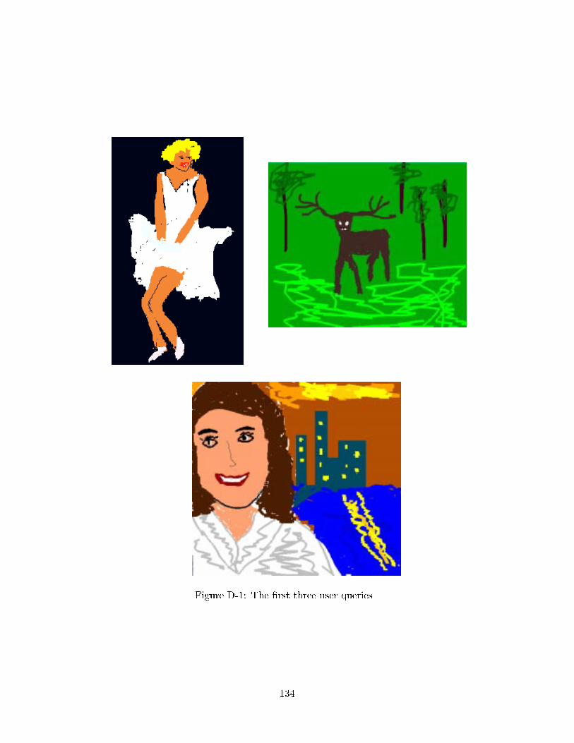
Figure D-1: The �rst three user queries.
134

Figure D-2: The second set of three user queries.
135

Figure D-3: The �rst set of database images.
136

Figure D-4: The second set of database images.
137

Figure D-5: The third set of database images.
138

139

140

141

142

143

144

Appendix E
Image User Queries and Matches
The queries listed here are based on the same query set as the queries in appendix D. These queries
highlight the methodology of region matching.
Two search screens are shown at nearly full size, and a third is shown shrunken. Each of these
displays a single query result. Although the query results are multiple pages long, only the top
matches are displayed in this appendix.
In the search screen, the query region is shown in the �rst row of the display. The regions which
match the best are listed in sequential order, from best to worst, below this. Because the image
which contains the query region was inserted into the database before searching in both cases, the
query region also shows up as its own best match. This is a good sanity check of the functionality
of the comparison mechanisms employed.
Two color and three shape matching metrics are used for region comparison. These are, in order
from left to right: color histograms, color mappings, volume-based representation, segment-based
representation, and angle-based representation.
The top value displayed in each screen �eld is the computed match of that region with the query
region based on the given representation. The second value is the normalized value for the given
representation space. The goodness value of each region is the weighted sum of these values. For
the queries shown, the default weights of 1 for every representation space were used.
145

146

147

148

149

150

Bibliography
[1] Nina Amenta, Marshal Bern, and Manolis Kamvysselis. A new voronoi-based surface recon-
struction algorithm. ACM Siggraph, August 1998. A provably correct algorithm for recon-
structing the shape of an object from samples on its boundary.
[2] Serge Belongie, Chad Carson, Hayit Greenspan, and Jitendra. Malik. Color- and texture-based
image segmentation using em and its application to content-based image retrieval. Interna-
tional Conference on Computer Vision (ICCV) `98, 1998. This is the short version of [5], in
which it was included almost verbatim.
[3] Egon Brunswik and Joe Kamiya. Ecological cue-validity of \proximity" and of other gestalt
factors. American Journal of Psychology, 66:20{32, 1953. Looks at whether Gestalt principles
apply to real image contexts by looking at some �lm sections.
[4] H. H. B�ultho�, S. Y. Edelman, and M. J. Tarr. How are three-dimensional objects represented
in the brain? Technical Report 5, Max-Planck-Institut f�ur biologische Kybernetik, T�ubingen,
Germany, 1994. Also published in 1995 in Cerebral Cortex, 5(3), pp. 247-260. This paper is
among several published by these three authors, in combination or separately, in the early
90's, on the topic of whether visual objects are stored with 2-D or 3-D representations in the
human brain.
[5] Chad Carson, Serge Belongie, Hayit Greenspan, and Jitendra. Malik. Color- and texture-
based image segmentation using em and its application to image querying and classi�cation.
Submitted to IEEE Transactions on Pattern Analysis and Machine Intelligence, 1999. This
paper is in review as of the time of the writing. It is an in-depth description of the Blobworld
content-based image indexing tool.
151

[6] Chad Carson, Megan Thomas, Serge Belongie, Joseph M. Hellerstein, and Jitendra Malik.
Blobworld: A system for region-based image indexing and retrieval. Visual Information Sys-
tems `99, 1999. One of several papers describing the Blobworld image indexing system.
[7] P. S. Churchland and T. J. Sejnowski. The Computational Brain. MIT Press, Cambridge,
Massachusetts, 1992. A computational look at neuroscience.
[8] David A. Forsyth and Margaret M. Fleck. Body plans. Computer Vision and Pattern Recog-
nition (CVPR) '97, Puerto Rico, June 1997. This paper is related to the Blobworld system.
It describes the thinking which later went into building the system.
[9] David A. Forsyth, Jitendra Malik, Margaret M. Fleck, Hayit Greenspan, Thomas Leung, Serge
Belongie, Chad Carson, and Chris Bleger. Finding pictures of objects in large collections of
images. European Conference on Computer Vision (ECCV) '96 Workshop on Object Recogni-
tion for Computer Vision., 1996. This paper is related to the Blobworld system. It describes
the thinking which later went into building the system.
[10] James J. Gibson. Observations on active touch. Psychological Review, 69(6):477{491, 1962.
A very thought-provoking paper on the di�erence between actively seeking out sensory input
and just receiving sensory input. The argument is that the only way to really get a sense of
the world is by the former, not the latter. A must-read.
[11] L. Van Gool, J. Wagemans, J Vandeneede, and A. Oosterlinck. Similarity extraction and
modeling. IEEE International Conference on Computer Vision, pages 530{534, 1990. A
discussion of computing similarity between shapes based on their points of in ection and of
zero curvature.
[12] A. Gupta and R. Jain. Visual information retrieval. Communications of the Association
for Computing Machinery, 40(5):70{79, 1997. This paper discusses image transformation
techniques, limited applications and data query methods.
[13] B. K. P. Horn. Robot Vision. MIT Press, Cambridge, Massachusetts, 1986. The classic
book on computational approaches to vision, with a very strong mathematical handling of the
subject.
152

[14] B. K. P. Horn and B. G. Schunk. Determining optical ow. Arti�cial Intelligence, 17:185{203,
1981. This is one of the most well-known descriptions of the computations required by an
optical ow algorithm. It is cited even in recent publications on the topic.
[15] Laurent Itti, Christof Koch, and Ernst Niebur. A model of saliency-based visual attention
for rapid scene analysis. IEEE Transactions on Pattern Analysis and Machine Intelligence
(PAMI), 20(11):1254{1259, 1998. A model based on the early visual system in primates. The
focus of interest is the issue of how to compute the salient locations in an input image. In
primate vision, this is where attention is drawn and therefore potentially the section which
should be segmented with the most care in an image indexing system.
[16] D. J. Jobson, Z. Rahman, and G. A. Woodell. A multi-scale retinex for bridging the gap
between color images and the human observation of scenes. IEEE Transactions on Image
Processing: Special Issue on Color Processing, July 1997. This article discusses an application
based on the retinex theory which allows a nearly illumination-invariant description of an
image. This article glosses over most implementation details.
[17] D. J. Jobson, Z. Rahman, and G. A. Woodell. Properties and performance of a center/surround
retinex. IEEE Transactions on Image Processing, March 1997. The retinex theory as applied
to image color enhancement is discussed. Although a potentially useful image pre-processing
step, this was not applied in the Imagina system.
[18] Manolis Kamvysselis. Two-dimensional polygon morphing using the extended gaussian image.
http://mit.edu/manoli/ecimorph/, December 1997. Morphs two polygons by mapping edges
to weights on the unit circle and transforming one set of weights to another.
[19] Panayiotis Kamvysselis. Recursive expectation-maximization, an algorithm for segmentation.
Masters thesis, Massachusetts Institute of Technology (MIT), Department of Electrical Engi-
neering and Computer Science, June 1998. A model-based segmentation algorithm for recursive
Expectation-Maximization (EM). Demonstrates superior results to prior EM algorithms. It is
guaranteed to terminate, is deterministic, and requires no prior knowledge of the number of
classi�cation clusters.
[20] P. J. Kellman and M. E. Arterbury. The Cradle of Knowledge. MIT Press, Cambridge,
Massachusetts, 1998. An in-depth look at the experimental cognitive science literature on
153

infant cognition. This book is a good overview. Several chapters discuss object and scene
recognition, directly and indirectly.
[21] P. J. Kellman and E. S. Spelke. Perception of partly occluded objects in infancy. Cognitive
Psychology, 15:483{524, 1983. Addresses the question of when infants consider a display to
contain one object, and when infants consider a display to contain two objects, given that the
connection between two visible parts of some object is hidden. The bottom line: motion, not
color and form, are used in object segmentation early on.
[22] Robert Lagani�ere. Morphological corner detection. In 6th International Conference on Com-
puter Vision, pages 280{285, Bombay, India, January 1998. IEEE, Narosa Publishing House.
A paper describing a corner detection algorithm based on a form of template matching called
mathematical morphology.
[23] Edwin Land. An alternative technique for the computation of the designator in the retinex
theory of color vision. In Proceedings of the National Academy of Science, pages 3078{3080,
1986. This is one of Land's later papers on retinex. This reference is included as a starting
point for readers who may be more familiar with his earlier writings on the topic.
[24] Al�es Leonardis, Alok Gupta, and Ruzena Bajcsy. Segmentation as the search for the best
description of the image in terms of primitives. IEEE International Conference on Computer
Vision, pages 121{125, 1990. An older paper on implementations of image segmentation.
[25] Pamela R. Lipson. Context and con�guration based scene classi�cation. Phd thesis, Mas-
sachusetts Institute of Technology (MIT), Department of Electrical Engineering and Computer
Science, 1996. This thesis is related to the topic presented in Chapter 7 of Pawan Sinha's PhD
thesis[39]. It discusses qualitative image descriptions more in depth, culminating with the use
of templates to do image classi�cation.
[26] Thomas Minka. An image database browser that learns from user interaction. Technical
Report 365, MIT Media Laboratory, 1996. Describes the Photobook image indexing tool in
great detail. This report is also listed as an MIT thesis for the degree of Master of Electrical
Engineering and Computer Science.
[27] W. Niblack, R. Barber, W. Equitz, M. Flickner, D. Glasman, D. Petkovic, and P. Yanker. The
qbic project: Querying images by content using color, texture and shape. SPIE Proc. Storage
154

and Retrieval for Image and Video Databases, pages 173{187, 1993. One of the many papers
describing IBM's QBIC project.
[28] R. Parasuraman, editor. The Attentive Brain. MIT Press, Cambridge, Massachusetts, 1998.
Neuroscience with a focus on the universality of attention.
[29] Zoran Pe�cenovi�c, Minh Do, Serge Ayer, and Martin Vetterli. New methods for image retrieval.
In Proceedings of the International Congress on Imaging Science, September 1998. A summary
of most recent approaches to content-based image indexing. A good starting point on current
literature on the topic.
[30] Alex Pentland. Wearable intelligence. Scienti�c American, 276(1), 1998. A general overview
of his work. This paper contains no useful technical speci�cs.
[31] Alex Pentland, Rosalind W. Picard, and Stan Sclaro�. Photobook: Tools for content-based
manipulation of image databases. International Journal of Computer Vision, 18(3):233{254,
1996. An overview of Photobook, which is a system for image storage, indexing and retrieval,
with some technical details.
[32] M. A. Peterson and B. S. Gibson. Object recognition contributions to �gure-ground orga-
nization: Operations on outlines and subjective contours. Perception and Psychophysics,
56(5):551{564, 1994. This paper looks at whether outlines and subjective contours enable
�gure-ground perception. They argue that object recognition is based on edges determined
during early visual processing.
[33] Photo and Media Finder of AltaVista. http://image.altavista.com/, 1998. An image searching
and thumbnail preview front end to AltaVista.
[34] Aparna Lakshmi Ratan. The role of �xation and visual attention in object recognition. Techni-
cal Report 1529, MIT Arti�cial Intelligence Laboratory, January 1995. Although �xation and
visual attention are interesting topics, the discussion of the use of color for image segmentation
in chapter 3 of the report proved to be of most use to the Imagina project.
[35] M. D. Rugg, editor. Cognitive Neuroscience. MIT Press, Cambridge, Massachusetts, 1997. A
neuroscience textbook: a must-have for a feel of the current understanding of brain functioning.
155
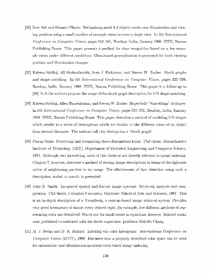
[36] Erez Sali and Shimon Ullman. Recognizing novel 3-d objects under new illumination and view-
ing position using a small number of example views or even a single view. In 6th International
Conference on Computer Vision, pages 153{161, Bombay, India, January 1998. IEEE, Narosa
Publishing House. This paper presents a method for class recognition based on a few exam-
ple views under di�erent conditions. Class-based generalization is presented for both viewing
position and illumination changes.
[37] Kaleem Siddiqi, Ali Shokoufandeh, Sven J. Dickinson, and Steven W. Zucker. Shock graphs
and shape matching. In 6th International Conference on Computer Vision, pages 222{229,
Bombay, India, January 1998. IEEE, Narosa Publishing House. This paper is a follow-up to
[38]. In it the authors propose the usage of the shock graph description for 2-D shape matching.
[38] Kaleem Siddiqi, Allen Tannenbaum, and Steven W. Zucker. Hyperbolic \Smoothing" of shapes.
In 6th International Conference on Computer Vision, pages 215{221, Bombay, India, January
1998. IEEE, Narosa Publishing House. This paper describes a method of modeling 2-D shapes
which results in a series of descriptions which are similar to the di�erent views of an object
from several distances. The authors call this description a \shock graph".
[39] Pawan Sinha. Perceiving and recognizing three-dimensional forms. Phd thesis, Massachusetts
Institute of Technology (MIT), Department of Electrical Engineering and Computer Science,
1995. Although very interesting, most of this thesis is not directly relevant to image indexing.
Chapter 7, however, discusses a method of storing image descriptions in terms of the lightness
ratios of neighboring patches in an image. The e�ectiveness of face detection using such a
description, scaled to match, is presented.
[40] John R. Smith. Integrated spatial and feature image systems: Retrieval, analysis and com-
pression. Phd thesis, Columbia University, Graduate School of Arts and Sciences, 1997. This
is an in-depth description of a VisualSeek, a content-based image retrieval system. Provides
very good treatments of almost every related topic; for example, �ve di�erent methods of rep-
resenting color are described! Watch out for small errors in equations, however. Related works
were published co-authored with his thesis supervisor, professor Shih-Fu Chang.
[41] M. J. Swain and D. H. Ballard. Indexing via color histograms. International Conference on
Computer Vision (ICCV), 1990. Discusses how a properly described color space can be used
for orientation- and illumination-invariant color-based image indexing.
156

[42] M. J. Swain and D. H. Ballard. Color indexing. International Journal of Computer Vision,
7(1):11{32, 1991. A more mature version of [41].
[43] Georges Thines, Alan Costall, and George Butterworth, editors. Michotte's Experimental
Phenomenology of Perception. L. Erlbaum Associates, Hillsdale, N.J., 1991. This is a re-
edition of Albert Michotte's classic work. It can be found listed under either the editors'
names or under Michotte. Only the section on the amodal completion of perceptual structures
was looked at.
[44] A. Treisman and G. Gelade. A feature integration theory of attention. Cognitive Psychology,
12:97{136, 1980. Part of a long line of work by A. Treisman dealing with the pre-attentive
selection of features.
[45] Shimon Ullman. High-Level Vision. MIT Press, Cambridge, Massachusetts, 1996. Although it
concentrates on Ullman's work, it is a very good summary of the current state of understanding
of human visual processes.
[46] Francisco J. Varela, Evan Thompson, and Eleanor Rosch. The Embodied Mind: Cognitive
Science and Human Experience. MIT Press, Cambridge, Massachusetts, 1991. The sections of
interest are the ones on Rosch's work in particular.
[47] Virage. http://www.virage.com/, 1998. Virage Inc partnered with Altavista in providing the
visual similarity search of the AltaVista Photo and Media Finder.
[48] James Ze Wang, Gio Wiederhold, Oscar Firschein, and Sha Xin Wei. Wavelet-based image
indexing techniques with partial sketch retrieval capability. In Proceedings of the Fourth Forum
on Research and Technology Advances in Digital Libraries (ADL'97), Washington, D.C., May
1997. A slightly di�erent approach to content-based image indexing. As a bonus, wavelets
allow compression of the images.
[49] Max Wertheimer. Readings in Perception, selected and edited by David C. Beardslee and
Michael Wertheimer, selection 8, pages 115{135. Van Nostrand, Princeton, N.J., 1958. This
short paper, \Principles of Perceptual Organization", provides a quick coverage of gestalt
principles with respect to visual input.
157


![[Ralph Thorn] Combat Knife Throwing a New Approac(Bookos.org)](https://static.fdocuments.us/doc/165x107/552d57924a795970668b46d1/ralph-thorn-combat-knife-throwing-a-new-approacbookosorg.jpg)