1

Image Processing Toolbox

Matlab

2

1. Introduction

• Matlab Platform for Image/Video Processing• Image Acquisition and Sampling• Some Applications• Aspects of Image Processing• Grayscale/RGB/Index Color Images• Image Format Conversion• Basics of Image Display

3

Matlab Platform for Image/Video Processing

• Matrix Laboratory• Internal Data Structure and Matrix Operators are natural for Image

Processing• Intrinsic Matrix Operators are implemented with highly efficient

Algorithms• Simple access to OS file system and interactive operations over the

Working Space simplifies algorithm development• Ready to use Signal/Image Processing Toolboxes contain highly

efficient functions which cover modern and even novel algorithms• Matlab Language allows Highly Structured Object Oriented

Programming Environment• The Full list of Image Processing Toolbox functions – help images

4

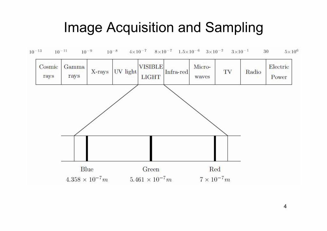
Image Acquisition and Sampling

5

Image Acquisition and Sampling

6

Image Acquisition and Sampling

• Browsing File System[Fname,Fdir]=uigetfile( ‘*.jpg’,’Click on Image file’ );

a = imread(Fname);

7

Image Acquisition and Samplingfigure; imshow(a);

8

Image Acquisition and Samplingimfinfo([Fdir,F1name])

ans =

Filename: [1x80 char]FileModDate: '25-May-2010 09:06:44'

FileSize: 976879Format: 'jpg'

FormatVersion: ''Width: 2592Height: 1944

BitDepth: 24ColorType: 'truecolor'

FormatSignature: ''NumberOfSamples: 3

CodingMethod: 'Huffman'CodingProcess: 'Sequential'

Comment: {}ImageDescription: ' '

Make: 'NIKON 'Model: 'E5600 '

Orientation: 1XResolution: 300YResolution: 300

ResolutionUnit: 'Inch'Software: 'E5600v1.0 'DateTime: '2010:05:25 09:06:44 '

YCbCrPositioning: 'Co-sited'DigitalCamera: [1x1 struct]

disp(ans.FileSize)976879

9

Image Acquisition and Sampling

B=rgb2gray(a); figure; imshow(b); figure; mesh(B); colormap(gray);

10

Some Applications and Examples• Medical

– Inspection and interpretation of images obtained from X-rays, MRI or CAT scans

– analysis of cell images, of chromosome karyotypes.

• Agriculture– Satellite/aerial views of land, for example to determine how much land

is being used for different purposes, or to investigate the suitability of different regions for different crops,

– inspection of fruit and vegetables distinguishing good and freshproduce from old.

• Industry– Automatic inspection of items on a production line,– inspection of paper samples.

• Law enforcements– Fingerprint analysis,– sharpening or de-blurring of speed-camera images.

11

Some Aspects of Image Processing• Image enhancement

– sharpening or de-blurring an out of focus image,– highlighting edges,– improving image contrast, or brightening an image,– removing noise.

• Image restoration– removing of blur caused by linear motion,– removal of optical distortions,– removing periodic interference.

• Image segmentation– finding lines, circles, or particular shapes in an image,– in an aerial photograph, identifying cars, trees, buildings, or roads.

• Image Geometry Transformation– affine transformation

12

Some Applications and Examples

13

Some Applications and Examples

14

Some Applications and Examples

15

Some Applications and Examples

16

Grayscale Images

17

RGB Images

18

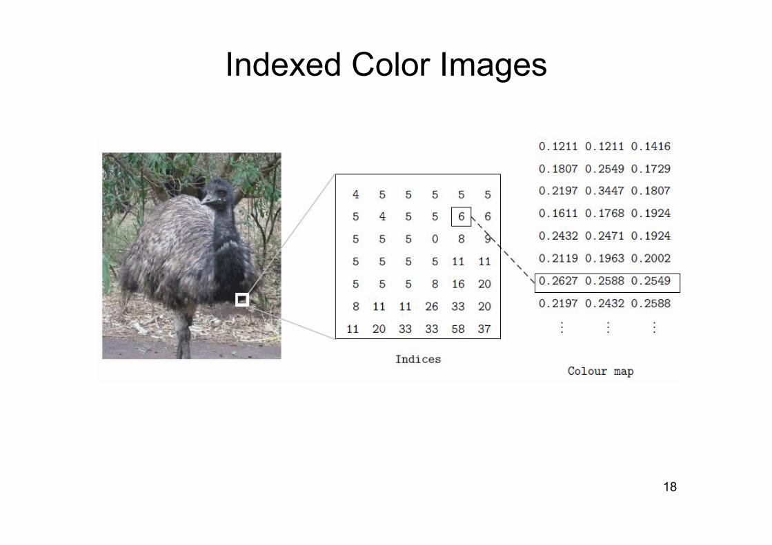
Indexed Color Images

19

Indexed Color Imagesfigure; imshow(a); [y,map]=rgb2ind(a,256);

Figure; image(y); colormap(map)

500 1000 1500 2000 2500

200

400

600

800

1000

1200

1400

1600

1800

20

Data Types & Image Format Conversion

21

Basics of Image Displayimpixelinfo

22

Basics of Image Displayimprofile; grid on

23

Basics of Image DisplayImage

c=imread(‘cameraman.tif’);figure; image(c);

50 100 150 200 250

50

100

150

200

250

figure; image(c);colormap(gray);

50 100 150 200 250

50

100

150

200

250

n=size(unique(c));figure; image(c);colormap(gray(n));

50 100 150 200 250

50

100

150

200

250

24

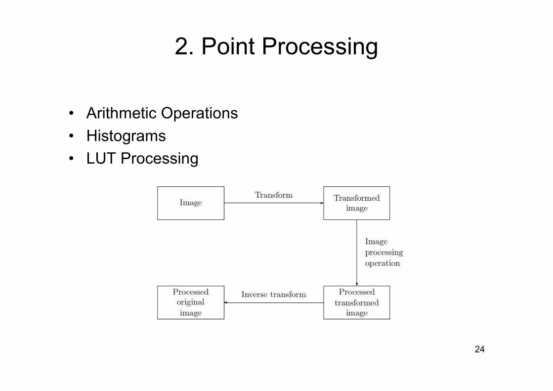
2. Point Processing

• Arithmetic Operations• Histograms• LUT Processing

25

Arithmetic Operationsb=imread(‘blocks.tif’’);

b1=uint8(double(b)+128);Or b1=imadd(b,128);

b2=imsubstruct(b,128);

imaddimsubstractimmultiplyimdivideimcomplement

26

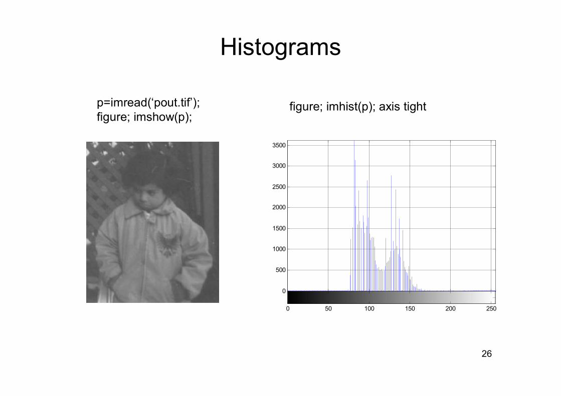
Histograms

0

500

1000

1500

2000

2500

3000

3500

0 50 100 150 200 250

figure; imhist(p); axis tightp=imread(‘pout.tif’);figure; imshow(p);

27

Histograms

figure; imhist(p1); axis tight

0

500

1000

1500

2000

2500

3000

3500

0 50 100 150 200 250

p1=histeq(p);figure; imshow(p1);

Histogram Equalization – histeq()

28

Histograms

A=adapthisteq(I,’clipLimit’,0.02,’Distribution’,’rayleigh’);figure; imshow(A);

Adaptive Histogram Equalization – adapthisteq()

I=imread(‘tire.tif’);figure; imshow(I);

29

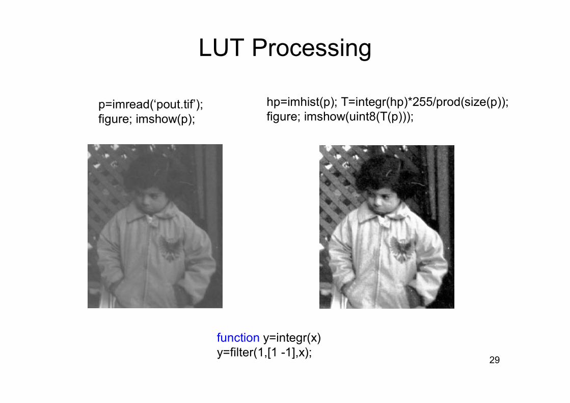
LUT Processing

hp=imhist(p); T=integr(hp)*255/prod(size(p));figure; imshow(uint8(T(p)));

p=imread(‘pout.tif’);figure; imshow(p);

function y=integr(x)y=filter(1,[1 -1],x);

30

3. Neighbourhood Processing

• Filtering in Matlab• Frequencies; Low and High Pass Filters• Edge sharpening• Non-linear Filters

31

Filtering in MatlabPerforming Spatial Filtering

32

Filtering in MatlabPerforming Spatial Filtering

33

Filtering in MatlabPerforming Spatial Filtering

34

Filtering in MatlabPerforming Spatial Filtering

35

Filtering in Matlab

36

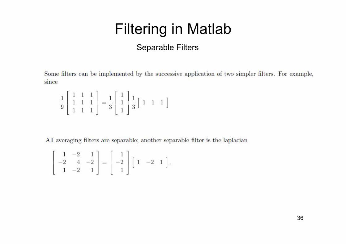
Filtering in MatlabSeparable Filters

37

Frequencies; Low and High Pass Filters

38

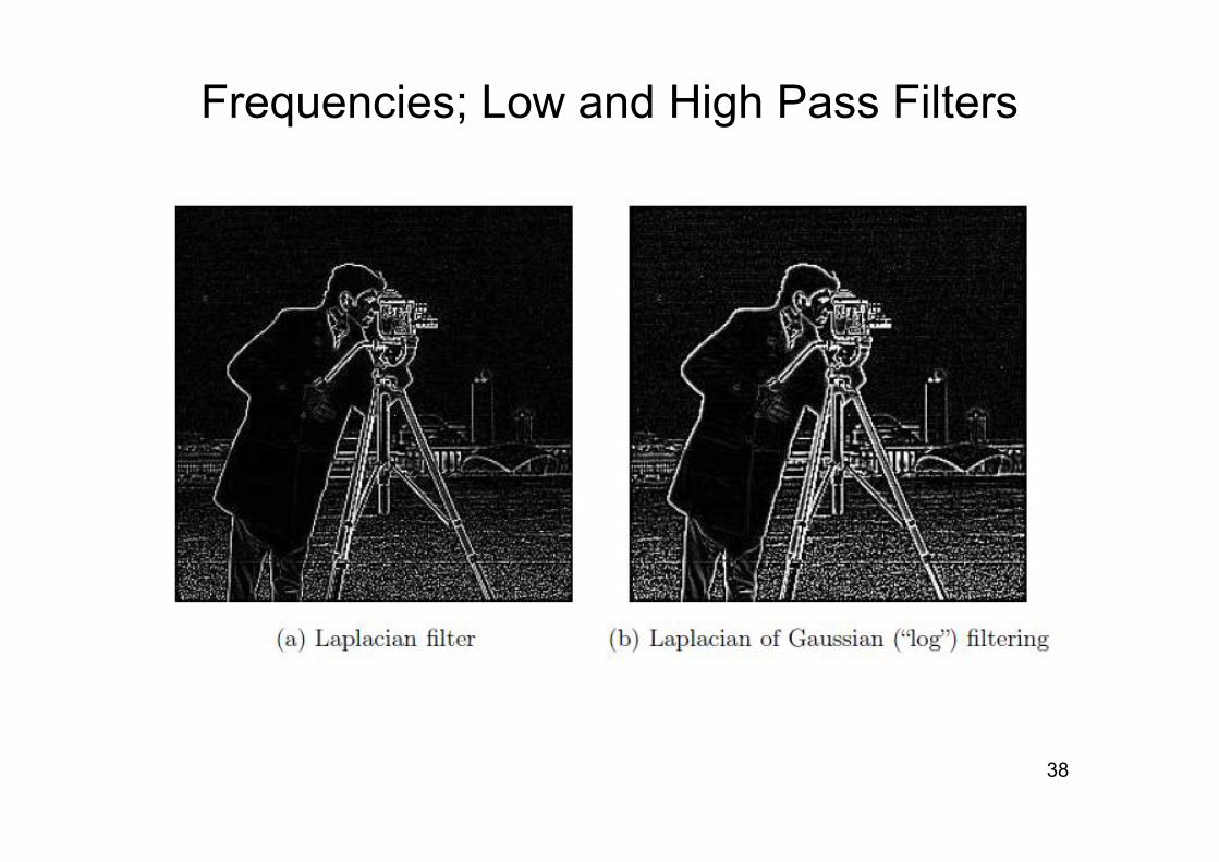
Frequencies; Low and High Pass Filters

39

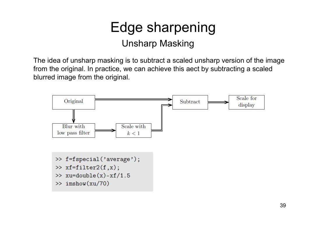
Edge sharpeningUnsharp Masking

The idea of unsharp masking is to subtract a scaled unsharp version of the image from the original. In practice, we can achieve this aect by subtracting a scaled blurred image from the original.

40

Edge sharpeningUnsharp Masking

41

Edge sharpeningUnsharp Masking

42

Edge sharpeningUnsharp Masking

43

Non-linear Filters

44

4. The Fourier Transform

• The 1D/2D discrete Fourier transform• Fourier transforms in Matlab• Fourier transforms of images• Matlab Programming Concepts• Filtering in the frequency domain

45

The 1D/2D discrete Fourier transform

46

Fourier transforms in Matlab

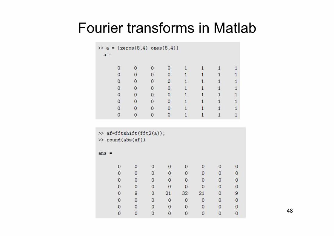
• fft which takes the DFT of a vector,• ifft which takes the inverse DFT of a vector,• fft2 which takes the DFT of a matrix,• ifft2 which takes the inverse DFT of a matrix,• fftshift which shifts a transform

47

Fourier transforms in Matlab

48

Fourier transforms in Matlab

49

Fourier transforms of images

50

Fourier transforms of imagesExamples

51

Fourier transforms of imagesExamples

52

Fourier transforms of imagesExamples

53

Fourier transforms of imagesExamples

54

Matlab Programming Concepts

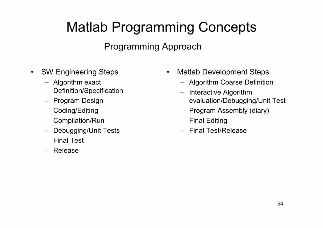
• SW Engineering Steps– Algorithm exact

Definition/Specification– Program Design– Coding/Editing– Compilation/Run– Debugging/Unit Tests– Final Test– Release

• Matlab Development Steps– Algorithm Coarse Definition– Interactive Algorithm

evaluation/Debugging/Unit Test– Program Assembly (diary)– Final Editing– Final Test/Release

Programming Approach

55

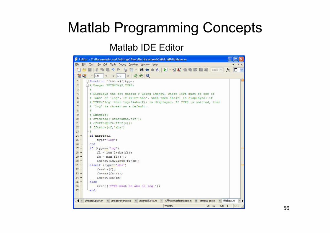
Matlab Programming ConceptsProgramming Features

• Matlab traditional variable: double precision complex matrix (2D)• Matlab Image/Video oriented variables: int8, uint8, frame, NaN, etc;• Matlab structures: cell-arrays, functions, inline function, etc;• Extended help: comment block, help, doc, lookfor, whos, which, etc;• Program flow controls: for...end, if…end, while…end, switch…end, etc;• Objects: figure, plot, imshow, avifile, imaqhwinfo, videoinput, @file, etc;• File access functions: fprinf, imread, read, write, fopen, fclose, etc;• DDE operators: ddeinit, xlsfinfo, xlsread, xlswrite, csvread, etc;• GUI editor;• Build-in benchmarking: tic, toc, clock, cputime, memory, etc;• Half-compiler (second run is faster!)

56

Matlab Programming ConceptsMatlab IDE Editor

57

Matlab Programming ConceptsProgramming Stile (recommendations)

• Maximal use of matrix notation• Avoid program flow controls (no for-loops!)• Maximal use logical matrix operation• “Vectorized” file access• Standard m-file structure:

– function [y1,y2]=myfunc(x1,x2,x3)%myfunc – brief description …% continue help block%Syntax: [y1,y2]=myfunc(x1,x2,x3), where%x1 – first argument …

%Author: … (not visible by help)Function body:a=x1; %comment

58

Filtering in the frequency domain

59

Filtering in the frequency domainIdeal LPF (the same dimensions as image)

Filter Application

60

Filtering in the frequency domain

Filter Application

Ideal HPF (the same dimensions as image)

61

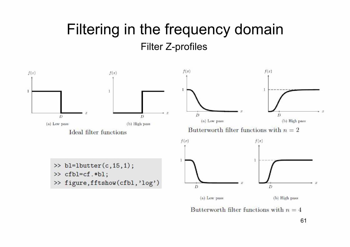
Filtering in the frequency domainFilter Z-profiles

62

Filtering in the frequency domainButterworth Filters

63

Filtering in the frequency domainGaussian Filter

64

Filtering in the frequency domainLP Gaussian Filter

65

Filtering in the frequency domainHP Gaussian Filter

66

5. Image Restoration

• Noise• Cleaning salt and pepper noise• Cleaning Gaussian noise• Removal of periodic noise• Debluring

67

NoiseSalt and pepper noise Gaussian noise (additive)

Speckle noise (multiplicative) Periodic noise

68

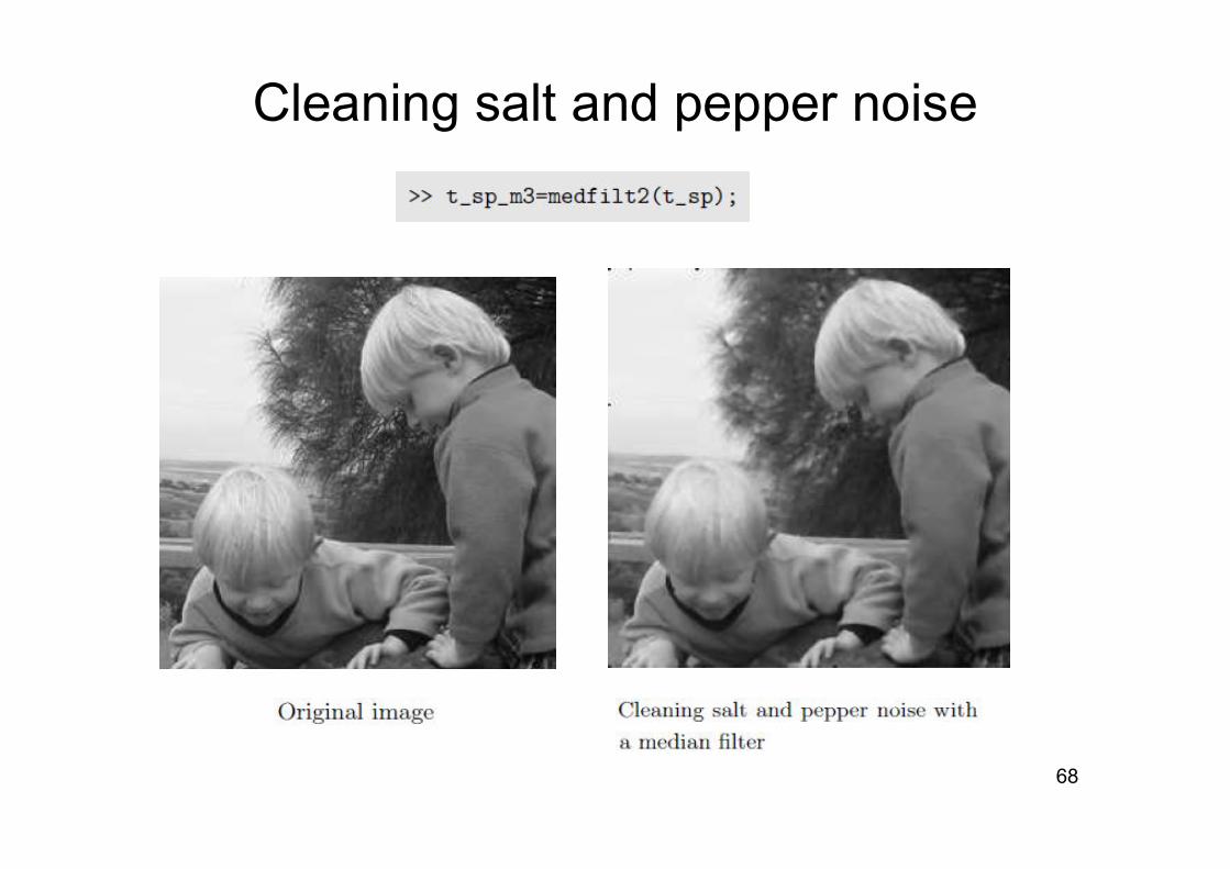
Cleaning salt and pepper noise

69

Cleaning Gaussian noiseImage averaging

It may sometimes happen that instead of just one image corrupted with Gaussian noise, we have many different copies of it. An example is satellite imaging; if a satellite passes over the same spot many times, we will obtain many different images of the same place.

70

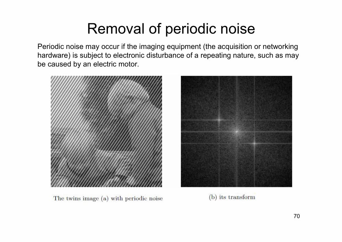
Removal of periodic noisePeriodic noise may occur if the imaging equipment (the acquisition or networking hardware) is subject to electronic disturbance of a repeating nature, such as may be caused by an electric motor.

71

Removal of periodic noiseBand reject Filtering

72

Removal of periodic noiseNotch Filtering

73

Debluring

The result of motion blur

74

DebluringTo deblur the image, we need to divide its transform by the transform corresponding to the blur filter. This means that we first must create a matrix corresponding to the transform of the blur:

Now we can attempt to divide by this transform.

75

DebluringWe can constrain the division by only dividing by values which are above a certain threshold.

76

6. Image Segmentation

• Thresholding• Edge Detection• The Hough transform

Segmentation refers to the operation of partitioning an image into component parts, or into separate objects.

77

Thresholding

78

Edge Detection

• Matlab Function edge• Use the following techniques:

– Prewitt– Roberts– Sobel– Laplacian of Gaussian (‘log’)– Zero-crossings of a laplacian– the Marr-Hildreth method

79

Edge Detection

I=imread('circuit.tif');figure; imshow(I);

BW1 = edge(I,‘log');figure; imshow(BW1);

80

Edge Detection

I=imread('circuit.tif');figure; imshow(I);

BW2 = edge(I, ‘sobel');figure; imshow(BW2);

81

Edge Detection

I=imread('circuit.tif');figure; imshow(I);

BW3 = edge(I, 'canny');figure; imshow(BW3);

82

The Hough transformIf the edge points found by the edge detection methods are SPARSE, the resulting edge image may consist of individual points, rather than straight lines or curves. Thus in order to establish a boundary between the regions, it might be necessary to FIT a LINE to those points.

Line definition for Hough Transform

83

The Hough transformRGB=imread(‘gantrycrane.png’);figure; imshow(RGB);

BW=edge(rgb2gray(RGB),’canny’);figure; imshow(BW);

44

44.5

45

45.5

46

-5000

5000

20

40

60

80

Thetar

Cou

nts

[H,T,R]=hough(BW,’Theta’,[44:0.5:46]);

RGB size is [264 400 3]

84

7. Image Geometry Transformation

• Affine Transform• Projective Transforms• Composite Transform

85

Affine Transform0.5 0 00.5 2 00 0 1

T =

I=imread(‘cameraman.tif’);figure; imshow(I);

T=maketform(‘affine’,[.5 0 0;.5 2 0;0 0 1]);transI = imtransform(I,T);figure, imshow(transI);