Image Denoising Using Scale Mixtures of Gaussians in the Wavelet Domain
28
Image Denoising Using Scale Mixtures of Gaussians in the Wavelet Domain Portilla , J . (Universidad de Granada); Strela , V. (Drexel University); Wainwright , M.J . (University of California, Berkeley); Simoncelli , E.P . (New York University); Transactions on: Image Processing, IEEE Journals
description
Image Denoising Using Scale Mixtures of Gaussians in the Wavelet Domain. Portilla , J . ( Universidad de Granada ); Strela , V. (Drexel University); Wainwright , M.J . ( University of California, Berkeley ); Simoncelli , E.P . ( New York University ); - PowerPoint PPT Presentation
Transcript of Image Denoising Using Scale Mixtures of Gaussians in the Wavelet Domain
Image Denoising Using Scale Mixtures of Gaussians in the Wavelet Domain
Portilla, J.(Universidad de Granada); Strela, V.(Drexel University); Wainwright, M.J.(University of California, Berkeley); Simoncelli, E.P.(New York University);
Transactions on: Image Processing, IEEE Journals

Outline• Introduction• Image probability model
– Gaussian scale mixtures– GSM model for wavelet coefficients– Prior density for multiplier
• Image denoising– Bayes least squares estimator– Local Wiener estimate– Posterior distribution of the multiplier
• Results– Implementation– Denoising digital camera images

Introduction
• Survey of image denoising techniques:

Hard thresholding: if (coef[i] <= thresh) coef[i] = 0.0;Soft thresholding: if (coef[i] <= thresh) coef[i] = 0.0; else coef[i] = coef[i] - thresh;
Image probability model
• An image decomposed into oriented subbands at multiple scales by wavelet transform.
• We assume the coefficients within each local neighborhood are characterized by a Gaussian scale mixture (GSM) [3] model.
• The neighborhood may include coefficients from nearby scales and orientations.
[3] D Andrews and C Mallows, “Scale mixtures of normal distributions,” J. Royal Stat. Soc., vol. 36, pp. 99–, 1974.

-Gaussian scale mixtures
• We denote as xc the center coefficient.
• We denote as x the vector of coefficient xc and its neighborhood coefficients (scales and orientations).
• The vector x characterized by a Gaussian scale mixture (GSM) model:
– u: zero-mean Gaussian vector.– z: independent positive scalar random variable.
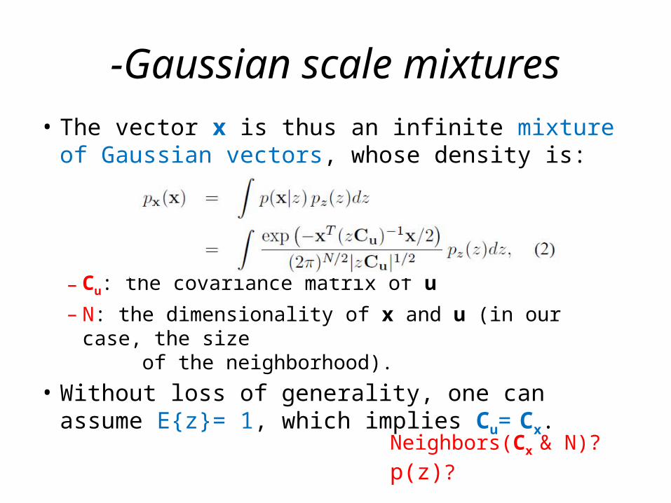
-Gaussian scale mixtures• The vector x is thus an infinite mixture of Gaussian
vectors, whose density is:
– Cu: the covariance matrix of u– N: the dimensionality of x and u (in our case, the size
of the neighborhood).• Without loss of generality, one can assume E{z}= 1,
which implies Cu= Cx.Neighbors(Cx & N)? p(z)?
-GSM model for wavelet coefficients
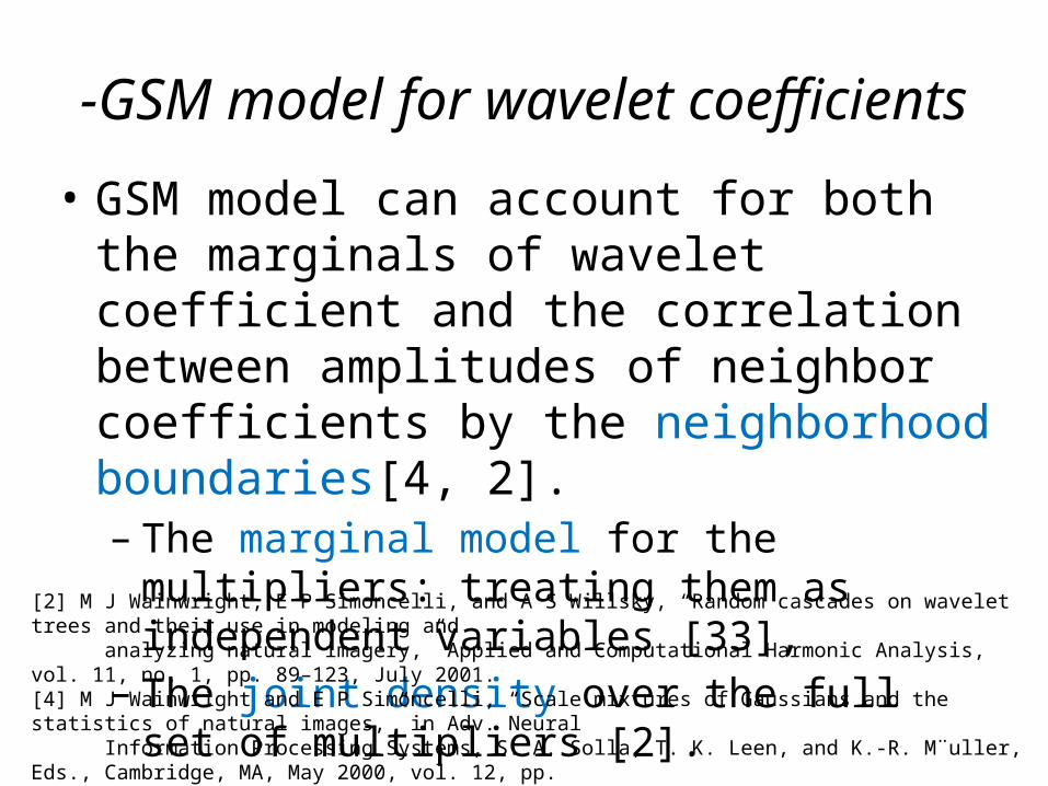
• GSM model can account for both the marginals of wavelet coefficient and the correlation between amplitudes of neighbor coefficients by the neighborhood boundaries[4, 2].– The marginal model for the multipliers: treating
them as independent variables [33],– The joint density over the full set of multipliers [2].
[2] M J Wainwright, E P Simoncelli, and A S Willsky, “Random cascades on wavelet trees and their use in modeling and analyzing natural imagery,” Applied and Computational Harmonic Analysis, vol. 11, no. 1, pp. 89–123, July 2001.[4] M J Wainwright and E P Simoncelli, “Scale mixtures of Gaussians and the statistics of natural images,” in Adv. Neural Information Processing Systems, S. A. Solla, T. K. Leen, and K.-R. M¨uller, Eds., Cambridge, MA, May 2000, vol. 12, pp. 855–861, MIT Press.[33] V Strela, “Denoising via block Wiener filtering in wavelet domain,” in 3rd European Congress of Mathematics, Barcelona, July 2000, Birkh¨auser Verlag.

-GSM model for wavelet coefficients
• An alternative approach is to use a GSM as a local description.
• The model implicitly defines a local Markov model, described by the conditional density of a coefficient of its surrounding neighborhood.
• The choice of neighborhood is described in section “Implementation”.
Get Neighbors(Cx & N).
-Prior density for multiplier
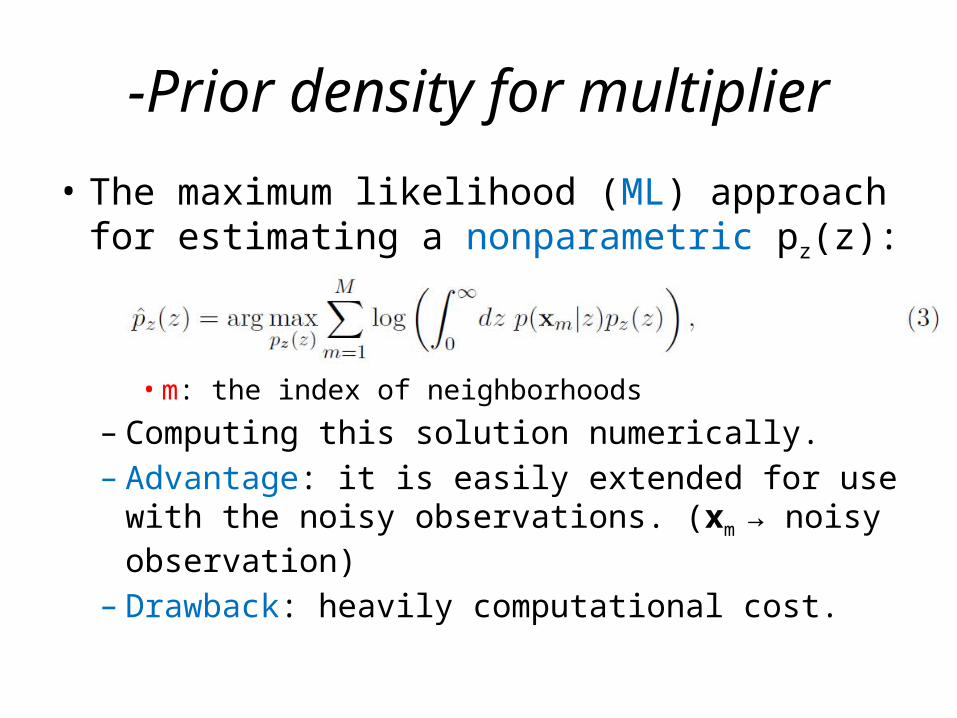
• The maximum likelihood (ML) approach for estimating a nonparametric pz(z):
• m: the index of neighborhoods– Computing this solution numerically.– Advantage: it is easily extended for use with the noisy
observations. (xm → noisy observation)– Drawback: heavily computational cost.

-Prior density for multiplier– Results:

-Prior density for multiplier• Noninformative prior (Jeffrey’s prior) [36] :
– Jeffrey’s prior:– Advantage: it does not require the fitting of any
parameters to the noisy observation.• Better denoising performance in image domain.
[36] G E P Box and C Tiao, Bayesian Inference in Statistical Analysis, Addison-Wesley, Reading, MA, 1992.Get p(z). Model completed.

Image denoising
(1) Decompose the image into pyramid subbandsat different scales and orientations;
(2) Denoise each subband;(3) Invert transform, obtaining the denoised
image.• We assume the image is corrupted by
independent additive Gaussian noise of known covariance.
• The noise and image contents are independent.

Image denoising
• A vector y corresponding to a neighborhood of N observed coefficients can be expressed as:
– Both u and w are zero-mean Gaussian vectors, with covariance matrices Cu and Cw.
• The density of y conditioned on z is a zero-mean Gaussian, with covariance Cy|z = zCu + Cw:

Image denoising• Since w is derived from the image through the
(linear) pyramid transformation, it is easily to compute the noise covariance matrix Cw.
• Taking the expectation of Cy|z over z yields:
• Choose E{z} = 1, resulting in:
• Ensure that Cu is positive semidefinite.(By performing an eigenvector decomposition and setting any negative eigenvalues to zero.)
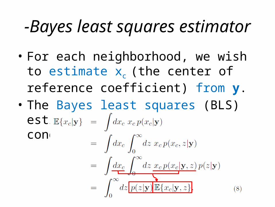
-Bayes least squares estimator
• For each neighborhood, we wish to estimate xc (the center of reference coefficient) from y.
• The Bayes least squares (BLS) estimate is just the conditional mean:
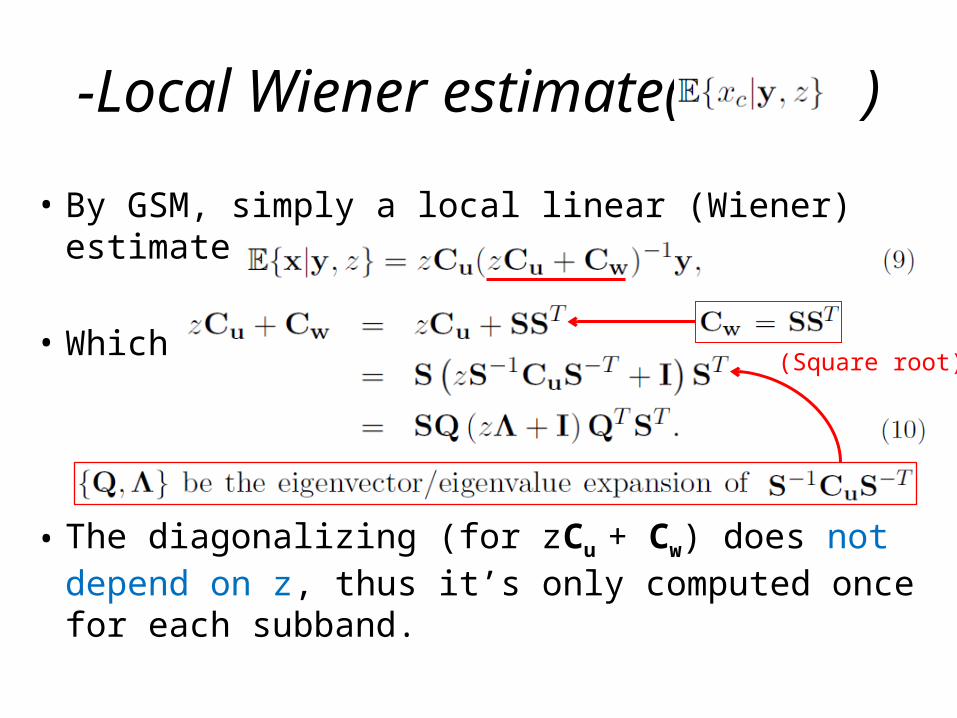
-Local Wiener estimate( )
• By GSM, simply a local linear (Wiener) estimate:
• Which
• The diagonalizing (for zCu + Cw) does not depend on z, thus it’s only computed once for each subband.
(Square root)
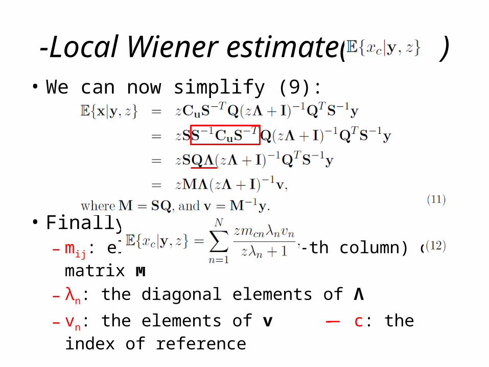
• We can now simplify (9):
• Finally: – mij: element(i-th row, j-th column) of matrix M– λn: the diagonal elements of Λ– vn: the elements of v -̶̶ c: the index of reference
-Local Wiener estimate( )
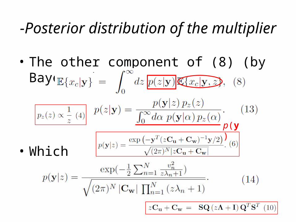
-Posterior distribution of the multiplier
• The other component of (8) (by Bayes rule):
• Whichp(y)

Summarizing our denoising algorithm

Results• Implementation:
– Decompose the image: The steerable pyramid[14]5 scales, 8 oriented highpass residual subbands, and one lowpass (non-oriented) residual band.
– Hand-optimized the neighborhood structure:A 3 × 3 region surrounding xc , together with the coefficient at the same location and orientation at the next coarser scale [19].
– Test on a set of 8-bit grayscale test images with additive Gaussian white noise at 10 different variances.
[14] E P Simoncelli,WT Freeman, E H Adelson, and D J Heeger, “Shiftable multi-scale transforms,” IEEE Trans Information Theory, vol. 38, no. 2, pp. 587–607, March 1992, Special Issue on Wavelets.[19] R W Buccigrossi and E P Simoncelli, “Image compression via joint statistical characterization in the wavelet domain,” IEEE Trans Image Proc, vol. 8, no. 12, pp. 1688–1701, December 1999.

Results


Results
[30] Xin Li and Michael T. Orchard, “Spatially adaptive image denoising under overcomplete expansion,” in IEEE Int’l Conf on Image Proc, Vancouver, September 2000.

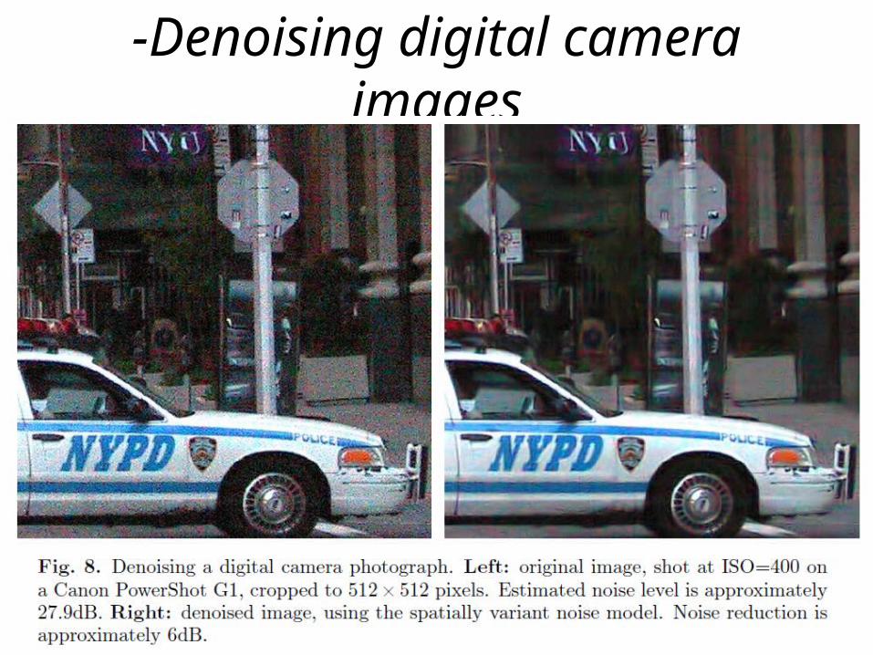
-Denoising digital camera images
• We obtain images from a Canon G1 digital camera (2160×1440 CCD quantized to 10 bits).
• The noise is strongly dependent on the signal:

-Denoising digital camera images
• In the subband domain, we assumed the following noise model:
– αx: the secondary multiplier of local noise variance. where E{αx} = 1 and it depends on pixel variance over a spatial neighborhood (see Appendix C).
• Once the values αx have been computed, then replace (z λn+1) in (14) and (12) with (z λn+αx).
-Denoising digital camera images
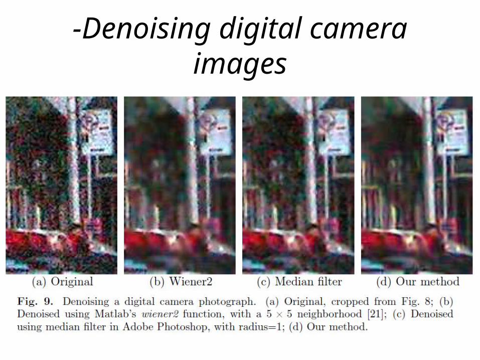
-Denoising digital camera images