Image Dehazing by Artificial Multiple-Exposure Image Fusion

A. Galdrana,∗

aINESC TEC Porto, R. Dr. Roberto Frias, 4200 Porto, Portugal

Abstract

Bad weather conditions can reduce visibility on images acquired outdoors, decreasing their visual quality. The image pro-cessing task concerned with the mitigation of this effect is known as image dehazing. In this paper we present a new imagedehazing technique that can remove the visual degradation due to haze without relying on the inversion of a physical modelof haze formation, but respecting its main underlying assumptions. Hence, the proposed technique avoids the need of esti-mating depth in the scene, as well as costly depth map refinement processes. To achieve this goal, the original hazy imageis first artificially under-exposed by means of a sequence of gamma-correction operations. The resulting set of multiply-exposed images is merged into a haze-free result through a multi-scale Laplacian blending scheme. A detailed experimentalevaluation is presented in terms of both qualitative and quantitative analysis. The obtained results indicate that the fusionof artificially under-exposed images can effectively remove the effect of haze, even in challenging situations where other cur-rent image dehazing techniques fail to produce good-quality results. An implementation of the technique is open-sourcedfor reproducibility (https://github.com/agaldran/amef_dehazing).

Keywords: Image Dehazing, Fog Removal, Multi-Exposure Image Fusion, Gamma Correction, Image Fusion, LaplacianPyramid

1. Introduction

Images acquired outdoors are sometimes degraded bya decrease in visibility caused by small particles suspendedin the atmosphere. This physical phenomenon is known ashaze or fog, and its main effect is the attenuation of the ra-diance along its path towards the camera. As a result, ac-quired images and videos suffer from loss of contrast andcolor quality degradation, limiting visibility on far away ar-eas in the scene. This lack of visibility can hinder the per-formance of computer vision systems designed to operateon clear conditions and also decreases visual pleasantnessof image contents for users of standard consumer cameras.

The task of restoring the visual quality of weather-degradedimages has been increasingly drawing attention in recent years.In this context, the image processing problem concerned withremoving the effect of foggy conditions is known as imagedehazing. The availability of effective image dehazing tech-niques can have a positive impact in computer vision tasksthat need to be performed in outdoor scenarios, such as surveil-lance [1], remote sensing [2, 3], or autonomous driving underbad-weather conditions [4].

Haze degradation is known to increase with respect todepth in the imaged scene. However, due to the ambiguityintroduced by the lack of depth information in two-dimensionalimages, early solutions to remove haze relied on external sources

∗Corresponding authorEmail address: adrian.galdran@inesctec.pt (A. Galdran)

of information [5, 6, 7]. Unfortunately, this external informa-tion is not usually available in generic situations, limiting theapplicability of this kind of techniques.

Single-image dehazing approaches were introduced toovercome this obstacle. A single-image dehazing techniqueassumes no external knowledge of the scene an image de-picts. However, since haze is a depth-dependent phenomenon,the resulting image degradation is spatially-variant, with dif-ferent areas of the image being more affected. In this situ-ation, unavailable depth information is typically alleviatedby resorting to physical models of haze formation. Unfortu-nately, even simplified physical models need to hold depthinformation, either implicitly or explicitly. As a result, mostexisting single-image dehazing methods impose prior infor-mation on the image the user expects to obtain, e.g. an in-creased contrast or less attenuated colors [8, 9].

The main contribution of this paper is an alternative sin-gle image dehazing method that employs physical models ofhaze formation only as an inspiration to understand char-acteristics of the image we expect to obtain. We considersingle-image haze removal as a spatially-varying contrast andsaturation enhancement problem on which different areasof the image require distinct levels of processing. Hence, anew image dehazing technique aiming at increasing visualquality only on those areas is built. This is achieved by ar-tificially underexposing the hazy image through a series ofgamma-correction operations. The resulting set of progres-sively underexposed images contains regions with increasedcontrast and saturation. To further account for the spatially-varying nature of weather degradation, a simple and efficient

Preprint submitted to Signal Processing March 26, 2018

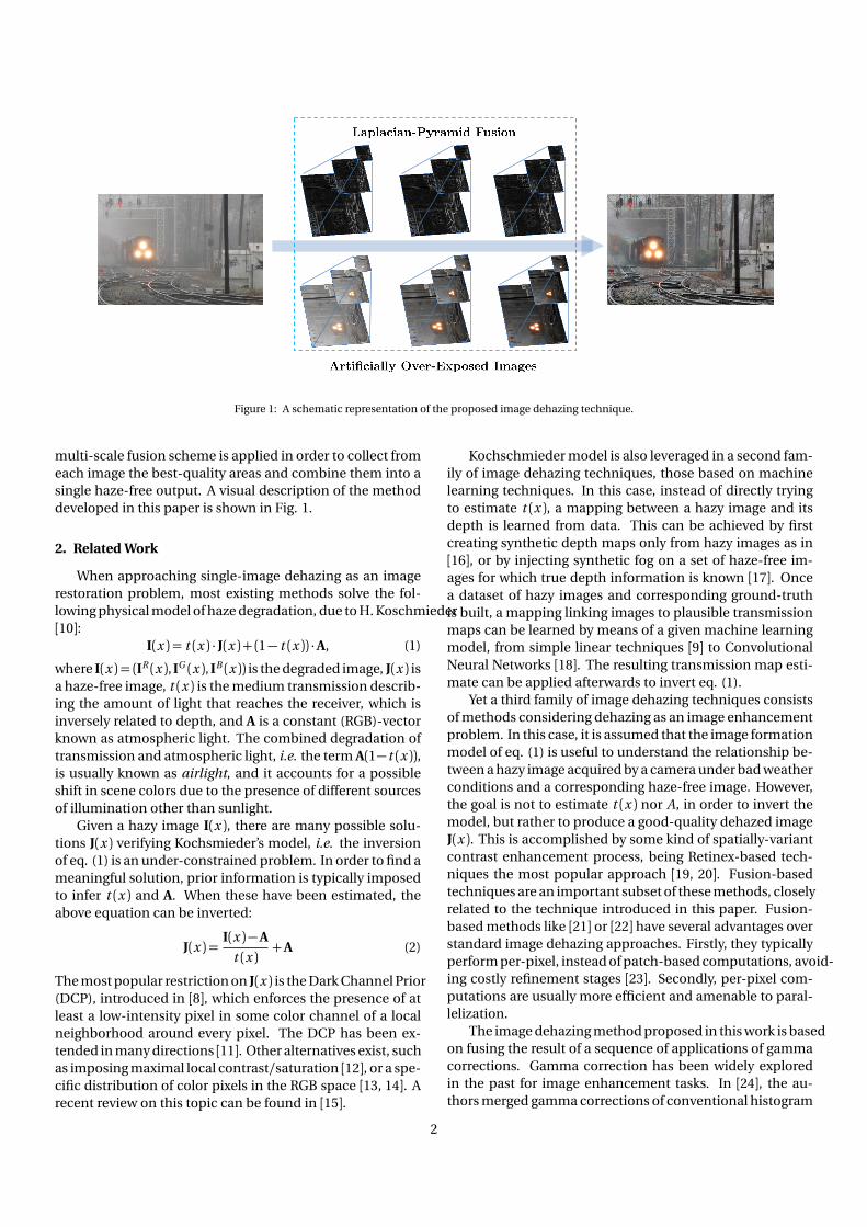
Figure 1: A schematic representation of the proposed image dehazing technique.

multi-scale fusion scheme is applied in order to collect fromeach image the best-quality areas and combine them into asingle haze-free output. A visual description of the methoddeveloped in this paper is shown in Fig. 1.

2. Related Work

When approaching single-image dehazing as an imagerestoration problem, most existing methods solve the fol-lowing physical model of haze degradation, due to H. Koschmieder[10]:

I(x ) = t (x ) · J(x ) + (1− t (x )) ·A, (1)

where I(x ) = (IR (x ), IG (x ), IB (x )) is the degraded image, J(x ) isa haze-free image, t (x ) is the medium transmission describ-ing the amount of light that reaches the receiver, which isinversely related to depth, and A is a constant (RGB)-vectorknown as atmospheric light. The combined degradation oftransmission and atmospheric light, i.e. the term A(1− t (x )),is usually known as airlight, and it accounts for a possibleshift in scene colors due to the presence of different sourcesof illumination other than sunlight.

Given a hazy image I(x ), there are many possible solu-tions J(x ) verifying Kochsmieder’s model, i.e. the inversionof eq. (1) is an under-constrained problem. In order to find ameaningful solution, prior information is typically imposedto infer t (x ) and A. When these have been estimated, theabove equation can be inverted:

J(x ) =I(x )−A

t (x )+A (2)

The most popular restriction on J(x ) is the Dark Channel Prior(DCP), introduced in [8], which enforces the presence of atleast a low-intensity pixel in some color channel of a localneighborhood around every pixel. The DCP has been ex-tended in many directions [11]. Other alternatives exist, suchas imposing maximal local contrast/saturation [12], or a spe-cific distribution of color pixels in the RGB space [13, 14]. Arecent review on this topic can be found in [15].

Kochschmieder model is also leveraged in a second fam-ily of image dehazing techniques, those based on machinelearning techniques. In this case, instead of directly tryingto estimate t (x ), a mapping between a hazy image and itsdepth is learned from data. This can be achieved by firstcreating synthetic depth maps only from hazy images as in[16], or by injecting synthetic fog on a set of haze-free im-ages for which true depth information is known [17]. Oncea dataset of hazy images and corresponding ground-truthis built, a mapping linking images to plausible transmissionmaps can be learned by means of a given machine learningmodel, from simple linear techniques [9] to ConvolutionalNeural Networks [18]. The resulting transmission map esti-mate can be applied afterwards to invert eq. (1).

Yet a third family of image dehazing techniques consistsof methods considering dehazing as an image enhancementproblem. In this case, it is assumed that the image formationmodel of eq. (1) is useful to understand the relationship be-tween a hazy image acquired by a camera under bad weatherconditions and a corresponding haze-free image. However,the goal is not to estimate t (x ) nor A, in order to invert themodel, but rather to produce a good-quality dehazed imageJ(x ). This is accomplished by some kind of spatially-variantcontrast enhancement process, being Retinex-based tech-niques the most popular approach [19, 20]. Fusion-basedtechniques are an important subset of these methods, closelyrelated to the technique introduced in this paper. Fusion-based methods like [21] or [22] have several advantages overstandard image dehazing approaches. Firstly, they typicallyperform per-pixel, instead of patch-based computations, avoid-ing costly refinement stages [23]. Secondly, per-pixel com-putations are usually more efficient and amenable to paral-lelization.

The image dehazing method proposed in this work is basedon fusing the result of a sequence of applications of gammacorrections. Gamma correction has been widely exploredin the past for image enhancement tasks. In [24], the au-thors merged gamma corrections of conventional histogram

2

equalization in order to achieve more effective contrast im-provement. In [25], an iterative method, automatically adaptedto the kind of degradation the image suffered, was proposed.Adaptive gamma correction was also adopted in [26], achiev-ing image content-dependence by devising a piece-wise powertransform through the incorporation of a cumulative histograminto a weighting distribution. However, even if these meth-ods are adaptive with respect to the image content and in-tensities, they remain global image transformations.

Other image processing tasks, e.g. color registration onimage sequences [27], have been approached with extensionsof basic gamma correction. However, image dehazing throughgamma correction has been hardly explored in the past. In[28], the authors proposed an adaptive gamma correctionscheme to refine the transmission map t (x ) before invert-ing model (1). The same idea was further improved in [29]through Laplacian-based techniques. In [30] gamma cor-rection was explored in conjunction with other contrast ad-justment techniques in order to rectify the intensities on thenegative of a hazy image in an efficient manner.

3. Artificial Multi-Exposure for Image Dehazing

The purpose of this paper is to build a spatially-varyingimage enhancement technique capable of removing the vi-sual effect of haze, bypassing the need of estimating trans-mission and airlight in eq. (1). However, there is underlyinginformation in Koschmieder’s model that can be useful tounderstand the kind of solution we should expect to obtain.To see this, let us consider an input hazy image I(x )with in-tensity values varying in [0, 1]. Then, any solution J(x ) to theimage dehazing problem needs to contain intensity valueslower than I(x ). This can be shown by simply rearrangingeq. (1) as:

t (x ) =A− I(x )A− J(x )

. (3)

Since t (x ) ∈ [0, 1], it follows from eq. (3) that A− I(x ) ≤ A−J(x ), and it can be concluded that J(x )≤ I(x )∀x .

According to the above observation, the technique intro-duced in this paper proposes to make use of the informationpresent in a set of over-exposed versions E= I1(x ), I2(x ), ..., In (x )of the original hazy image I(x ). Underexposing I(x ) will al-ways lead to the presence of decreased intensities. However,when I(x ) is globally underexposed, not every region on itcontains useful information, since insufficient exposure willdarken I(x ) too much. For this reason, all images in E arefused by means of a simple and efficient multiple-exposurefusion strategy relying on a Laplacian pyramid decomposi-tion of the set of over-exposed images. The resulting image isa haze-free version of I(x ). In the next sections, the differentsteps of this procedure are explained in detail.

3.1. Artificial Exposure Modification via Gamma CorrectionTransforms

In photography, exposure is defined as the amount of lightthat is allowed to enter the camera and reach the sensors

while acquiring an image [31]. Exposure can be adjusted dur-ing acquisition by varying the shutter speed of the cameraor its aperture, but it is typically hard to achieve a generallyoptimal exposure for any scene. Moreover, different areasof the imaged scene may require completely distinct expo-sures. The reason for this is the large dynamic range of thelight reaching the camera.

The difference between the brightest and darkest inten-sity values that a camera can register is called dynamic range.Most consumer cameras acquire low dynamic range images,covering few orders of magnitude. As a result, when captur-ing an image of a scene reflecting a high dynamic range oflight, a short exposure will allow the camera to correctly cap-ture details in the brightest areas of the image. However, onthe same conditions the camera will be unable of properlydepicting details in dark regions, and the corresponding im-age areas will be underexposed. In the same way, if a longexposure is used, dark region details will become apparent,but bright regions will become white, i.e. these areas will beoverexposed. Typically no single exposure time will be use-ful for both kind of regions.

In controlled illumination situations, a possible solutionis to shed artificial light on dark areas of the scene to reduceits dynamic range. A second approach consists of acquiringseveral images of the same scene under different exposuresand combining the information on all these images into asingle one containing sharp details both on bright and darkregions. This image processing problem is known as Multi-ple Exposure Fusion (MEF). MEF has been widely studied inthe past, and will be briefly discussed in section 3.2 below.

Unfortunately, most of the times the user has no con-trol on the illumination of the scene, or the image has al-ready been captured and stored, with no option to acquireextra differently exposed images on the same scene. In thiscase, an alternative solution consists of digitally adjustingthe exposure of the image. One of the simplest algorithmsto manipulate exposure is gamma correction. This consistsof globally modifying the intensities on an image followinga power-function transform:

I(x ) 7→α · I(x )γ, (4)

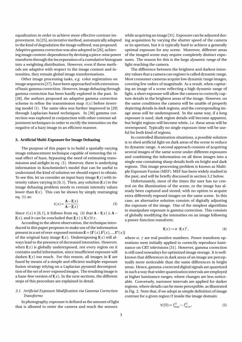
where α, γ are real positive numbers. Power transform op-erations were initially applied to correctly reproduce lumi-nance on CRT televisions [31]. However, gamma correctionis still used nowadays for optimized image storage. It is well-known that differences in dark areas of an image are percep-tually more noticeable than the same differences in brightareas. Hence, gamma-corrected digital signals are quantizedin such a way that wider quantization intervals are employedat higher luminance ranges, where changes are less notice-able. Conversely, narrower intervals are applied for darkerregions, where details can be more perceptible, as illustratedin Fig. 2. Note that, if we adopt as simple definition of imagecontrast for a given region Ω inside the image domain:

C (Ω) = I Ωmax− I Ωmi n , (5)

3

Figure 2: Dynamic range expansion/compression due to power transforms. Left: For γ < 1, brighter intensities are compressed while darker intensitiesare expanded. Right: conversely, for γ > 1, brighter intensities are allocated in a wider range after transformation, while darker intensities are mapped to acompressed interval.

where I Ωmax = maxI (x ) | x ∈ Ω and I Ωmin = minI (x ) | x ∈Ω, then it can be easily shown that, e.g. for γ > 1, given aregion containing bright values like in the right side of Fig.??, its contrast as measured by eq. (5), will be increased aftergamma correction, as shown in the right side of Fig. ??.

Optimal gamma-transformations and methods for esti-mating the γ-coefficient applied by a camera while storingan image have been explored in the past [32, 33]. However,in this paper we are interested in the visual effect that thistransformation can achieve on a digital image. In this sense,it is worth noting that gamma correction allows to globallyincrease or reduce exposure on a given image. Unfortunately,the application of eq. (4) leads to a global effect by whichproperly-exposed areas of the image become deteriorated,as shown in Fig. ??. However, as discussed in the next sec-tion, it is still possible to identify and fuse each of the im-age areas in order to obtain a fused image containing well-exposed areas across its entire domain.

3.2. Multi-Exposure Image Fusion

Since its introduction in [34], Multiple Exposure Fusion(MEF) has been largely investigated. However, the large ma-jority of MEF algorithms can be grouped into a single frame-work, that aims at finding the optimal weights Wk in the fol-lowing formula:

J(x ) =K∑

k=1

Wk (x )Ek (x ), (6)

where K is the number of differently exposed available im-ages Ek (x ), and J(x ) is a globally well-exposed image, result-ing from the combination of the different correctly-exposedareas in Ek . Weights Wk are normalized so that

∑

k Wk (x ) =1 ∀x , in order to keep the intensities of J(x ) in range. Somevariants of this approach avoid pixel-wise weighting by com-puting block-wise weights Wk , or solve eq. (6) in a trans-formed domain [35, 36].

Many techniques have been proposed to compute opti-mal Wk (x ) in eq. (6). Typically a multi-resolution strategy is

applied to avoid blending artifacts. This idea was introducedin [37]by means of a Laplacian Pyramid decomposition, andis recurrent in the literature. In [38], contrast, saturation, andwell-exposedness were employed as cues to detect correctlyexposed regions before performing a Laplacian multi-scalefusion. Also, in [39] gradient information and the structuretensor were used for the same purposes, and in [40, 41] edgerelevance was taken into consideration for either weightingimage areas or refining initial weight estimates. This can beachieved by means of different edge-preserving filters, e.g.bilateral or guided filters.

To avoid the appearance of visual artifacts, the multi-scaleapproach for image fusion based on the classical Laplacianpyramid [42] is also followed in this work. Let us assume thata set of maps Wk indicating the haze-free areas in each im-age is already available. Directly combining the input multi-exposed images into J(x ) following eq. (6) would result inhard transitions associated to weight maps’ borders. In or-der to combine different scales together, first a Gaussian pyra-mid is built for each weight map as:

Wik = ds2

Wi−1k

, (7)

where ds2[ · ] corresponds to an operator that convolves animage with a Gaussian kernel, and then downsamples it tohalf of its original dimensions. Iterating this process N timesproduces a set of progressively smaller and smoother weightmaps W1

k , W2k , . . . , WN

k .In a similar way, a Gaussian pyramid E1

k , E2k , . . . , EN

k isbuilt for each of the multi-exposed images Ek . Then, a Lapla-cian pyramid is constructed for each Ek through the follow-ing recursive formula:

Lik = Ei

k −us2

Ei+1k

, (8)

where us2[ · ] is an operator upsampling an image to twice itssize. In the above recursion, we define LN

k = ENk .

Since Lik (x ) captures the frequency content of the origi-

nal image at scale i , a multi-scale combination of all Ek (x )

4

J(x ) =us(m ,n )

L11(x ) ·W

11(x ) + . . .+L1

K (x )W1K (x )

+us(m ,n )

L21(x ) ·W

21(x ) + . . .+L2

K (x )W2K (x )

+ . . . (9)

+ . . . +us(m ,n )

LN1 (x ) ·W

N1 (x ) + . . .+LN

K (x )WNK (x )

=N∑

i=1

us(m ,n )

K∑

k=1

Lik (x ) ·W

ik (x )

,

where us(m ,n ) is the operator upsampling any given imageto the dimension of Ek . A schematic representation of theLaplacian decomposition scheme is given in Fig. (3).

It is worth noting that different weight selections Wk ineq. (6) will lead to distinct multi-scale blending results. How-ever, even simple choices can produce visually satisfactoryresults, as illustrated in Fig. 4. In the next section, a weightselection suitable for the task of image dehazing will be de-scribed.

3.3. Image Dehazing by Artificial Multiple Under-Exposed Im-age Fusion

As illustrated in Fig. (4a), artificially under/overexposingan image and fusing the results in a multi-scale fashion canintegrate well-exposed areas from each of the source images.However, for the purposes of this paper, it is of interest tomodel the fact that a solution to the haze formation in eq.(1) must always decrease intensities. For this reason, we pro-pose to compute only artificially under-exposed images, i.e.apply only γ> 1 in eq. (4). The global effect of this operationis a reduction in brightness. Moreover, subsequent applica-tions of gamma-correction with increasing values of γ canreveal useful visual information on a hazy image.

With the choice of γ > 1, it can be easily verified that thedehazed image computed by eq. (6) always fulfills the inten-sity decrease requirement. Consider a set of under-exposurefactors Γ = γ1,γ2, . . .γK | γk > 1. Since I(x ) ∈ [0, 1], thenI(x )γ

k< I(x ) for every pixel x . Due to the weights in eq. (6)

being normalized to sum up to 1, we have that:

J(x ) =K∑

k=1

Wk (x )Ik (x ) ≤K∑

k=1

Wk (x )I(x ) = I(x ) (10)

The effect of artificially under-exposing a hazy image isillustrated in Fig. (5a) and Figs. (5c) to (5l). It can be ap-preciated that, in a foggy image, well-exposed regions corre-sponding to areas closer to the camera can be found. More-over, by artificially under-exposing the initial image, hazy re-gions lying further away from the observer can be transformedinto well-saturated areas. The main drawback with globallyunder-exposing a hazy image is that areas that were initiallyof high visual quality in the first place are completely dark-ened. The goal thus becomes to build a suitable set of weightmaps modeling the presence of fog on each artificially under-exposed image in order to select from each of them regionswith the minimum haze density. Note that, by consideringthe original image also as an input for the fusion stage, theresult of the merging procedure explained below will retain

the ability of keeping regions of the image that were natu-rally dark in the initial scene. In this way, those regions willnot be discarded and will end up belonging to both the inputimage and the dehazed result.

It is well-known that one of the main visual effects of fogis the loss of contrast and saturation, and this has been widelyexploited in the literature. For instance, the popular DarkChannel Prior (DCP) imposes that, on a haze-free image, theremust always be a dark pixel in a neighborhood around eachpixel. Thus, the DCP proceeds by computing local minimaboth in space and RGB coordinates, building the Dark Chan-nel image as:

Jdark(x ) = minc∈R ,G ,B

miny ∈Ω(x )

Jc (y )

, (11)

where Ω(x ) is a patch centered at pixel x . By imposingthat the Dark Channel image contains only low intensities, itis possible to maximize both contrast and saturation on hazyregions. The reason for this is that verifying the DCP on hazyareas requires a local stretching of values in spatial neigh-borhoods (thereby expanding local contrast) combined witha local stretching of values in the RGB space (resulting in asaturation increase).

However, one of the main disadvantages of the DCP andits variants is that patch-wise computations are necessary inorder to robustly estimate contrast and saturation. This cre-ates the need of a costly post-processing of the haze map,typically achieved by the guided filter or similar techniques.To overcome these drawbacks, in this paper we simplify theapproach proposed in [38]. In this case, given a source im-age Ek (x ) = (ER

k (x ), EGk (x ), EB

k (x )), the contrast Ck (x ) at eachpixel x is measured as the absolute value of the response to asimple Laplacian filter, while saturation Sk (x ) on each pixelis estimated by the standard deviation across color channels:

Ck (x ) =∂ 2Ek

∂ x 2(x ) +

∂ 2Ek

∂ y 2(x ), (12)

Sk (x ) =∑

c∈R ,G ,B

Eck (x )−

ERk (x ) +EG

k (x ) +EBk (x )

3

2

. (13)

Finally, a haze map for each under-exposed image is obtainedby simply combining multiplicatively the contrast and satu-ration maps:

Wk (x ) =Ck (x ) ·Sk (x ) (14)

The resulting weights are inserted in eq. (6) and the Lapla-cian multi-scale fusion described in the previous section isperformed. This results in a haze-free image integrating well-contrasted regions with rich colors from each source image,as illustrated in Fig. 5b.

5

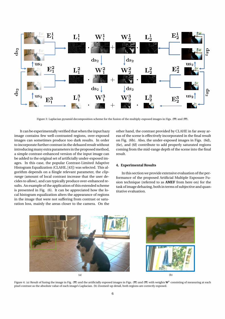
Figure 3: Laplacian pyramid decomposition scheme for the fusion of the multiply-exposed images in Figs. (??) and (??).

It can be experimentally verified that when the input hazyimage contains few well-contrasted regions, over-exposedimages can sometimes produce too dark results. In orderto incorporate further contrast in the dehazed result withoutintroducing many extra parameters in the proposed method,a simple contrast-enhanced version of the input image canbe added to the original set of artificially under-exposed im-ages. In this case, the popular Contrast-Limited AdaptiveHistogram Equalization (CLAHE, [43]) was selected. This al-gorithm depends on a ßingle relevant parameter, the clip-range (amount of local contrast increase that the user de-cides to allow), and can typically produce over-enhanced re-sults. An example of the application of this extended schemeis presented in Fig. (6). It can be appreciated how the lo-cal histogram equalization alters the appearance of regionsin the image that were not suffering from contrast or satu-ration loss, mainly the areas closer to the camera. On the

other hand, the contrast provided by CLAHE in far away ar-eas of the scene is effectively incorporated in the final resulton Fig. (6b). Also, the under-exposed images in Figs. (6d),(6e), and (6f) contribute to add properly saturated regionscoming from the mid-range depth of the scene into the finalresult.

4. Experimental Results

In this section we provide extensive evaluation of the per-formance of the proposed Artificial Multiple Exposure Fu-sion technique (referred to as AMEF from here on) for thetask of image dehazing, both in terms of subjective and quan-titative evaluation.

(a) (b)

Figure 4: (a) Result of fusing the image in Fig. (??) and the artificially exposed images in Figs. (??) and (??) with weights Wk consisting of measuring at eachpixel contrast as the absolute value of each image’s Laplacian. (b) Zoomed-up detail, both regions are correctly exposed.

6

(a) (b)

(c) (d) (e) (f) (g)

(h) (i) (j) (k) (l)

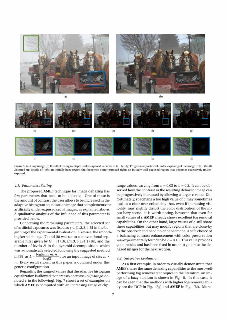
Figure 5: (a) Hazy image (b) Result of fusing multiple under-exposed versions of (a). (c)–(g) Progressively artificial under-exposing of the image in (a). (h)–(l)Zoomed-up details of: left) an initially hazy region that becomes better exposed right) an initially well-exposed region that becomes excessively under-exposed.

4.1. Parameters Setting

The proposed AMEF technique for image dehazing hasfew parameters that need to be adjusted. One of these isthe amount of contrast the user allows to be increased in theadaptive histogram equalization image that complements theartificially under-exposed set of images, as explained above.A qualitative analysis of the influence of this parameter isprovided below.

Concerning the remaining parameters, the selected setof artificial exposures was fixed as γ ∈ 1, 2, 3, 4, 5 in the be-ginning of the experimental evaluation. Likewise, the smooth-ing kernel in eqs. (7) and (8) was set to a conventional sep-arable filter given by G = [1/16, 1/4, 3/8, 1/4, 1/16], and thenumber of levels N in the pyramid decomposition, whichwas automatically selected following the suggested method

in [38] as L = log(min(m , n ))log(2) , for an input image of size m ×

n . Every result shown in this paper is obtained under thisgeneric configuration.

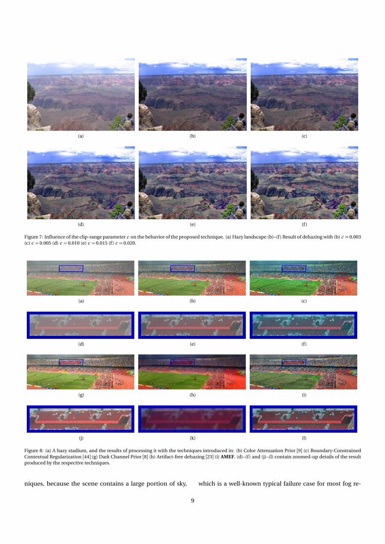
Regarding the range of values that the adaptive histogramequalization is allowed to increase/decrease (clip-range, de-noted c in the following), Fig. 7 shows a set of examples onwhich AMEF is computed with an increasing range of clip-

range values, varying from c = 0.03 to c = 0.2. It can be ob-served how the contrast in the resulting dehazed image canbe progressively increased by allowing a larger c value. Un-fortunately, specifying a too high value of c may sometimeslead to a clear over-enhancing that, even if increasing vis-ibility, may slightly distort the color distribution of the in-put hazy scene. It is worth noting, however, that even forsmall values of c AMEF already shows excellent fog removalcapabilities. On the other hand, large values of c still sharethese capabilities but may modify regions that are close-byto the observer and need no enhancement. A safe choice ofc balancing contrast enhancement with color preservationwas experimentally found to be c = 0.10. This value providesgood results and has been fixed in order to generate the de-hazed images for the next section.

4.2. Subjective Evaluation

As a first example, in order to visually demonstrate thatAMEF shares the same dehazing capabilities as the most well-performing fog removal techniques in the literature, an im-age of a hazy stadium is shown in Fig. 8. In this case, itcan be seen that the methods with higher fog-removal abil-ity are the DCP in Fig. (8g) and AMEF in Fig. (8i). More-

7

(a) (b)

(c) (d) (e) (f)

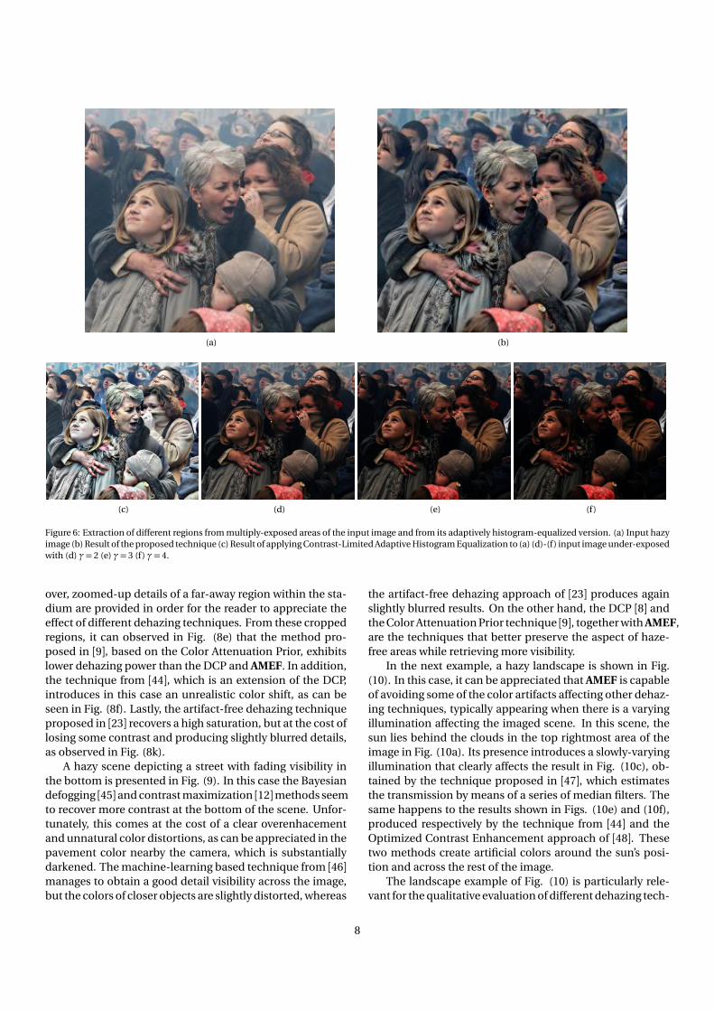
Figure 6: Extraction of different regions from multiply-exposed areas of the input image and from its adaptively histogram-equalized version. (a) Input hazyimage (b) Result of the proposed technique (c) Result of applying Contrast-Limited Adaptive Histogram Equalization to (a) (d)-(f) input image under-exposedwith (d) γ= 2 (e) γ= 3 (f) γ= 4.

over, zoomed-up details of a far-away region within the sta-dium are provided in order for the reader to appreciate theeffect of different dehazing techniques. From these croppedregions, it can observed in Fig. (8e) that the method pro-posed in [9], based on the Color Attenuation Prior, exhibitslower dehazing power than the DCP and AMEF. In addition,the technique from [44], which is an extension of the DCP,introduces in this case an unrealistic color shift, as can beseen in Fig. (8f). Lastly, the artifact-free dehazing techniqueproposed in [23] recovers a high saturation, but at the cost oflosing some contrast and producing slightly blurred details,as observed in Fig. (8k).

A hazy scene depicting a street with fading visibility inthe bottom is presented in Fig. (9). In this case the Bayesiandefogging [45]and contrast maximization [12]methods seemto recover more contrast at the bottom of the scene. Unfor-tunately, this comes at the cost of a clear overenhacementand unnatural color distortions, as can be appreciated in thepavement color nearby the camera, which is substantiallydarkened. The machine-learning based technique from [46]manages to obtain a good detail visibility across the image,but the colors of closer objects are slightly distorted, whereas

the artifact-free dehazing approach of [23] produces againslightly blurred results. On the other hand, the DCP [8] andthe Color Attenuation Prior technique [9], together with AMEF,are the techniques that better preserve the aspect of haze-free areas while retrieving more visibility.

In the next example, a hazy landscape is shown in Fig.(10). In this case, it can be appreciated that AMEF is capableof avoiding some of the color artifacts affecting other dehaz-ing techniques, typically appearing when there is a varyingillumination affecting the imaged scene. In this scene, thesun lies behind the clouds in the top rightmost area of theimage in Fig. (10a). Its presence introduces a slowly-varyingillumination that clearly affects the result in Fig. (10c), ob-tained by the technique proposed in [47], which estimatesthe transmission by means of a series of median filters. Thesame happens to the results shown in Figs. (10e) and (10f),produced respectively by the technique from [44] and theOptimized Contrast Enhancement approach of [48]. Thesetwo methods create artificial colors around the sun’s posi-tion and across the rest of the image.

The landscape example of Fig. (10) is particularly rele-vant for the qualitative evaluation of different dehazing tech-

8

(a) (b) (c)

(d) (e) (f)

Figure 7: Influence of the clip-range parameter c on the behavior of the proposed technique. (a) Hazy landscape (b)–(f) Result of dehazing with (b) c = 0.003(c) c = 0.005 (d) c = 0.010 (e) c = 0.015 (f) c = 0.020.

(a) (b) (c)

(d) (e) (f)

(g) (h) (i)

(j) (k) (l)

Figure 8: (a) A hazy stadium, and the results of processing it with the techniques introduced in: (b) Color Attenuation Prior [9] (c) Boundary-ConstrainedContextual Regularization [44] (g) Dark Channel Prior [8] (h) Artifact-free dehazing [23] (i) AMEF. (d)–(f) and (j)–(l) contain zoomed-up details of the resultproduced by the respective techniques.

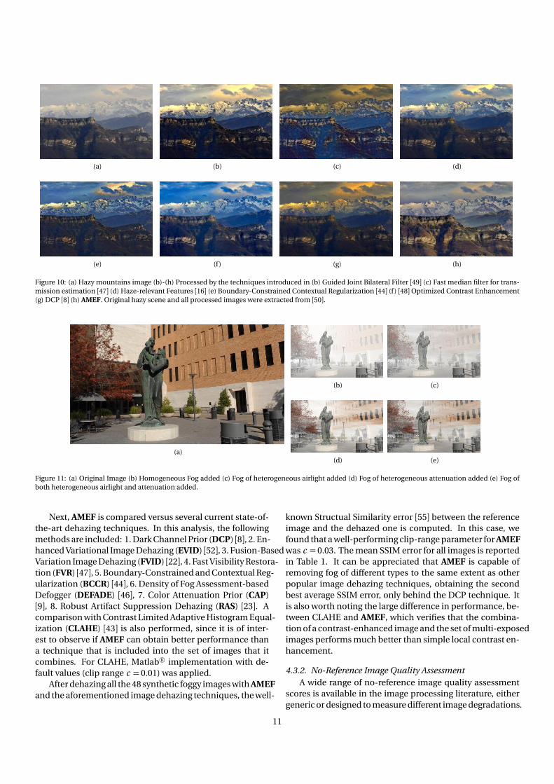
niques, because the scene contains a large portion of sky, which is a well-known typical failure case for most fog re-

9

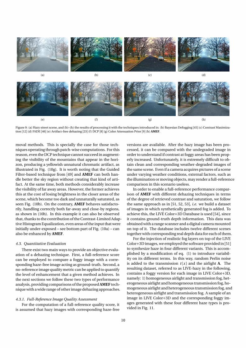
(a) (b) (c) (d)

(e) (f) (g) (h)

Figure 9: (a) Hazy street scene, and (b)–(h) the results of processing it with the techniques introduced in: (b) Bayesian Defogging [45] (c) Contrast Maximiza-tion [12] (d) FADE [46] (e) Artifact-free dehazing [23] (f) DCP [8] (g) Color Attenuation Prior [9] (h) AMEF.

moval methods. This is specially the case for those tech-niques operating through patch-wise computations. For thisreason, even the DCP technique cannot succeed in augment-ing the visibility of the mountains that appear in the hori-zon, producing a yellowish unnatural chromatic artifact, asillustrated in Fig. (10g). It is worth noting that the GuidedFilter-based technique from [49] and AMEF can both han-dle better the sky region without creating that kind of arti-fact. At the same time, both methods considerably increasethe visibility of far away areas. However, the former achievesthis at the cost of losing brightness in the closer areas of thescene, which become too dark and unnaturally saturated, asseen Fig. (10b). On the contrary, AMEF behaves satisfacto-rily, handling correctly both far-away and close-by regions,as shown in (10h). In this example it can also be observedthat, thanks to the contribution of the Contrast-Limited Adap-tive Histogram Equalization, even areas of the input that wereinitially under-exposed – see bottom part of Fig. (10a) – canalso be enhanced by AMEF.

4.3. Quantitative Evaluation

There exist two main ways to provide an objective evalu-ation of a dehazing technique. First, a full-reference scorecan be employed to compare a foggy image with a corre-sponding haze-free image acting as ground-truth. Second, ano-reference image quality metric can be applied to quantifythe level of enhancement that a given method achieves. Inthe next sections we follow these two types of performanceanalysis, providing comparisons of the proposed AMEF tech-nique with a wide range of other image dehazing approaches.

4.3.1. Full-Reference Image Quality AssessmentFor the computation of a full-reference quality score, it

is assumed that hazy images with corresponding haze-free

versions are available. After the hazy image has been pro-cessed, it can be compared with the undegraded image inorder to understand if contrast at foggy areas has been prop-erly increased. Unfortunately, it is extremely difficult to ob-tain clean and corresponding weather-degraded images ofthe same scene. Even if a camera acquires pictures of a sceneunder varying weather conditions, external factors, such asthe illumination or moving objects, may render a full-referencecomparison in this scenario useless.

In order to enable a full-reference performance compar-ison of AMEF with different dehazing techniques in termsof the degree of retrieved contrast and saturation, we followthe same approach as in [51, 52, 53], i.e. we build a datasetof images in which synthetically generated fog is added. Toachieve this, the LIVE Color+3D Database is used [54], sinceit contains ground-truth depth information. This data wasobtained with a range scanner and a digital camera mountedon top of it. The database includes twelve different scenestogether with corresponding real depth data for each of them.

For the injection of realistic fog layers on top of the LIVEColor+3D images, we employed the software provided in [51]to synthesize haze in four different variants. This is accom-plished by a modification of eq. (1) to introduce variabil-ity on its different terms. In this way, random Perlin noiseis added to the transmission t (x ) and the airlight A. Theresulting dataset, referred to as LIVE-hazy in the following,contains a foggy version for each image in LIVE Color+3D,namely: 1) homogeneous airlight and transmission fog, het-erogeneous airlight and homogeneous transmission fog, ho-mogeneous airlight and heterogeneous transmission fog, andheterogeneous airlight and transmission fog. A sample of animage in LIVE Color+3D and the corresponding foggy im-ages generated with these four different haze types is pro-vided in Fig. 11.

10

(a) (b) (c) (d)

(e) (f) (g) (h)

Figure 10: (a) Hazy mountains image (b)-(h) Processed by the techniques introduced in (b) Guided Joint Bilateral Filter [49] (c) Fast median filter for trans-mission estimation [47] (d) Haze-relevant Features [16] (e) Boundary-Constrained Contextual Regularization [44] (f) [48]Optimized Contrast Enhancement(g) DCP [8] (h) AMEF. Original hazy scene and all processed images were extracted from [50].

(a)

(b) (c)

(d) (e)

Figure 11: (a) Original Image (b) Homogeneous Fog added (c) Fog of heterogeneous airlight added (d) Fog of heterogeneous attenuation added (e) Fog ofboth heterogeneous airlight and attenuation added.

Next, AMEF is compared versus several current state-of-the-art dehazing techniques. In this analysis, the followingmethods are included: 1. Dark Channel Prior (DCP) [8], 2. En-hanced Variational Image Dehazing (EVID) [52], 3. Fusion-BasedVariation Image Dehazing (FVID) [22], 4. Fast Visibility Restora-tion (FVR) [47], 5. Boundary-Constrained and Contextual Reg-ularization (BCCR) [44], 6. Density of Fog Assessment-basedDefogger (DEFADE) [46], 7. Color Attenuation Prior (CAP)[9], 8. Robust Artifact Suppression Dehazing (RAS) [23]. Acomparison with Contrast Limited Adaptive Histogram Equal-ization (CLAHE) [43] is also performed, since it is of inter-est to observe if AMEF can obtain better performance thana technique that is included into the set of images that itcombines. For CLAHE, Matlab R© implementation with de-fault values (clip range c = 0.01) was applied.

After dehazing all the 48 synthetic foggy images with AMEFand the aforementioned image dehazing techniques, the well-

known Structual Similarity error [55] between the referenceimage and the dehazed one is computed. In this case, wefound that a well-performing clip-range parameter for AMEFwas c = 0.03. The mean SSIM error for all images is reportedin Table 1. It can be appreciated that AMEF is capable ofremoving fog of different types to the same extent as otherpopular image dehazing techniques, obtaining the secondbest average SSIM error, only behind the DCP technique. Itis also worth noting the large difference in performance, be-tween CLAHE and AMEF, which verifies that the combina-tion of a contrast-enhanced image and the set of multi-exposedimages performs much better than simple local contrast en-hancement.

4.3.2. No-Reference Image Quality AssessmentA wide range of no-reference image quality assessment

scores is available in the image processing literature, eithergeneric or designed to measure different image degradations.

11

Table 1: SSIM performance comparison of AMEF and other image dehazing techniques on the LIVE-hazy dataset. Resultssorted in ascending performance. Best method is marked green, second best is marked orange, and third best is marked red.

Method Mean SSIM Error Short Explanation

RASD [23] 0.507 Robust Artifact-Supression Dehazing

CLAHE [43] 0.671 Contrast-Limited Adaptive Histogram Equalization

CAP [9] 0.708 Imposes Color Attenuation Prior

DEFADE [46] 0.716 Learned Model of Fog presence + Fusion Scheme

FVID [22] 0.762 Fusion of the Iterates from EVID

FVR [47] 0.774 Fast Median Filter for Transmission Estimate

EVID [52] 0.780 Iterative Variational Image Dehazing

BCCR [44] 0.792 Contextual Transmission Regularization

DCP [8] 0.807 Imposes Dark Channel Prior

AMEF 0.795 Artificial Multiple Exposure Fusion.

However, it has been recently shown in [50] that most of thesequality metrics fail to capture the subjective opinion of hu-man observers regarding image appearance when evaluat-ing image dehazing techniques. Accordingly, to evaluate thedehazing capability of different techniques when comparedto AMEF, we apply the Fog Aware Density Evaluator (FADE)metric, introduced in [46], which is specifically designed forassessing image dehazing techniques. FADE is a learned qual-ity metric, supported by the computation of a set of fog-awarefeatures across two sets of images, foggy and fog-free, each ofthem containing 500 images. We selected the first set of hazyimages on which FADE was trained to compare the perfor-mance of the different techniques. This dataset is publiclyavailable 1. Results of the mean FADE values scored acrossthe considered 500 images, after processing them with thesame set of dehazing techniques as in previous section, areshown in Table 2.

First, it is important to remark that the best-performingclip-range value for AMEF in this case was found to be c =0.20. However, it must be noted that the FADE metric tendsto slightly reward an increased saturation, which agrees withthe better-performing greater clip-range value. Second, ananalysis of the performances reported in Table 2 reveals thatCLAHE performs substantially worse than AMEF also by thismetric, obtaining even a lower score than the original hazyimages, which confirms that simple local contrast enhance-ment is not enough to remove fog effects. Also, it is impor-tant to emphasize that the best performing technique un-der the FADE metric is the DEFADE method [46]. This is amachine learning technique that was trained employing thesame dataset on which these scores are computed. As a con-sequence, it is natural to expect a particularly good perfor-mance of DEFADE regarding this quality score. In this case,AMEF scores again the second best position, verifying its gooddehazing capability also when measured by a specialized no-reference quality metric.

1Accessible at http://live.ece.utexas.edu/research/fog/fade_defade.html

For reference, we also include in Table 2 the result of com-puting a no-reference quality metric designed for generic nat-ural images, CORNIA (Codebook Representation for No-ReferenceImage Assessment) [56]. In this case, we did not modify thedefault value of the clip-range parameter, which was kept asc = 0.10. We can see that AMEF still performs among thebest top image dehazing algorithms, ranking in the third po-sition.

4.4. Computational Performance Analysis

One critical aspect of image dehazing techniques is theexecution time the algorithm needs in order to process animage. In this section we provide a computational perfor-mance study to demonstrate the ability of AMEF to removehaze efficiently. In this analysis we consider some of the de-hazing techniques mentioned in Section 4.3.1. In addition,we incorporate to the analysis the Image Dehazing by Multi-Scale Fusion (MSF) technique from [21], the Visibility in BadWeather (VBW) method from [12], the Single Image Dehaz-ing (SID) technique introduced in [57], the Color-Lines (C-Lines)approach from [13], the Non-Local Image Dehazing(NLID) technique proposed in [14], the Haze-Relevant Fea-ture analysis (HRF) method from [16], and the DehazenetConvolutional Neural Network (DHZNet) introduced in [18].The resulting execution times for all these different techin-ques, extracted from [15]2, are reported in Table 3.

4.5. Robustness to JPEG compression artifacts

Another key aspect of image dehazing techniques is theirability to deal with compression artifacts that typically ap-pear on large bright areas with few contrast, e.g. white build-ings, portions of sky, etc. This is a typical failure scenariofor image dehazing techniques that carry out a per-patch

2Experiments in this reference were run using a desktop with a XeonE5 3.5GHz CPU and 16GB of RAM. Runtimes for FVID and AMEF were ob-tained by running the methods locally, in a desktop computer of the samespecifications.

12

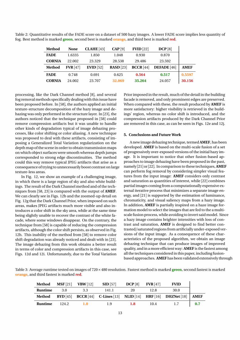
Table 2: Quantitative results of the FADE score on a dataset of 500 hazy images. A lower FADE score implies less quantity offog. Best method is marked green, second best is marked orange, and third best is marked red.

Method None CLAHE [43] CAP [9] FVID [22] DCP [8]

FADE 1.6335 1.850 1.048 0.930 0.870

CORNIA 22.002 23.329 28.538 29.486 23.592

Method FVR [47] EVID [52] RASD [23] BCCR [44] DEFADE [46] AMEF

FADE 0.748 0.691 0.625 0.564 0.517 0.5597

CORNIA 24.002 23.707 32.069 35.264 24.057 30.156

processing, like the Dark Channel method [8], and severalfog removal methods specifically dealing with this issue havebeen proposed before. In [58], the authors applied an initialtexture-structure decomposition of the hazy image and de-hazing was only performed in the structure layer. In [23], theauthors noticed that the technique proposed in [58] couldremove compression artifacts but it was unable to handleother kinds of degradation typical of image dehazing pro-cesses, like color shifting or color aliasing. A new techniquewas proposed to deal with these artifacts, consisting of im-posing a Generalized Total Variation regularization on thedepth map of the scene in order to obtain transmission mapson which object surfaces were smooth whereas depth jumpscorresponded to strong edge discontinuities. The methodcould this way remove typical JPEG artifacts that arise as aconsequence of trying to unnecessarily boost contrast on largetexture-less areas.

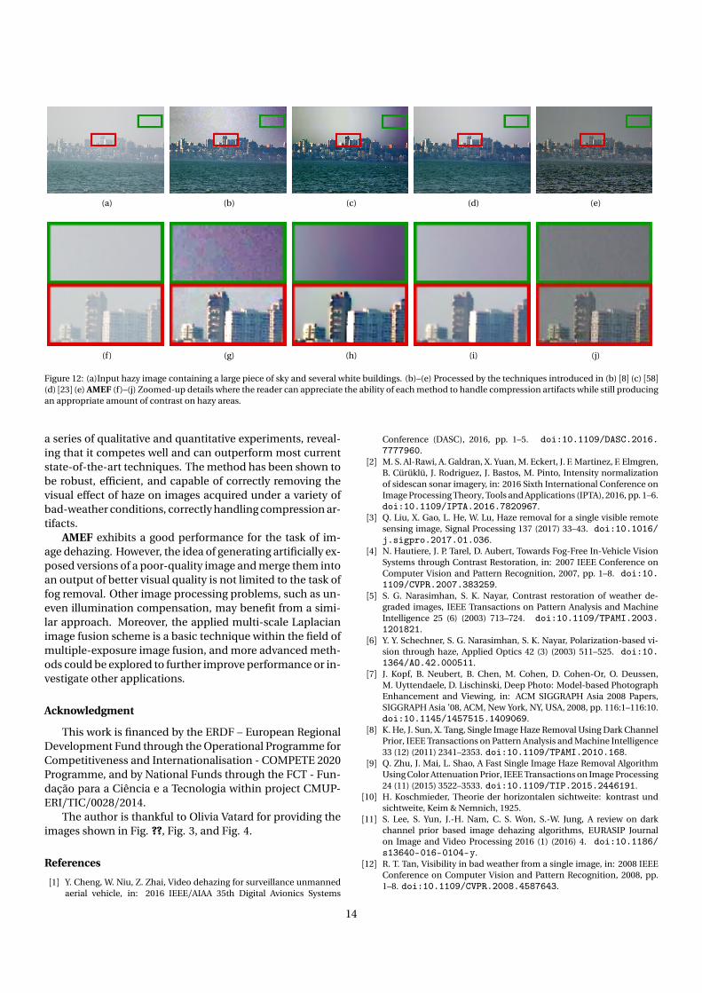
In Fig. 12, we show an example of a challenging image,in which there is a large region of sky and also white build-ings. The result of the Dark Channel method and of the tech-niques from [58, 23] is compared with the output of AMEF.We can clearly see in Figs. 12b and the zoomed-up detail onFig. 12g that the Dark Channel Prior, when imposed on suchareas, makes JPEG artifacts much more visible and also in-troduces a color shift in the sky area, while at the same timebeing slightly unable to recover the contrast of the white fa-cade, where some windows disappear. On the contrary, thetechnique from [58] is capable of reducing the compressionartifacts, although the color shift persists, as observed in Fig.12h. This inability of the method from [58] to remove colorshift degradation was already noticed and dealt with in [23].The image dehazing from this work obtains a better resultin terms of color and compression artifacts in this case, seeFigs. 12d and 12i. Unfortunately, due to the Total Variation

Prior imposed in the result, much of the detail in the buildingfacade is removed, and only prominent edges are preserved.When compared with these, the result produced by AMEF ismore satisfactory: higher visibility is retrieved in the build-ings’ region, whereas no color shift is introduced, and thecompression artifacts produced by the Dark Channel Priorare removed in this case, as can be seen in Figs. 12e and 12j.

5. Conclusions and Future Work

A new image dehazing technique, termed AMEF, has beendeveloped. AMEF is based on the multi-scale fusion of a setof progressively over-exposed versions of the initial hazy im-age. It is important to notice that other fusion-based ap-proaches to image dehazing have been proposed in the past,namely [21]or [22]. In comparison to these techniques, AMEFcan perform fog removal by considering simpler visual fea-tures from the input image: AMEF considers only contrastand saturation as quantities of interest, while [22] combinespartial images coming from a computationally expensive ex-ternal iterative process that minimizes a separate image en-ergy, and [21] is supported by the estimation of luminance,chromaticity, and visual saliency maps from a hazy image.In addition, AMEF is partially inspired on a haze image for-mation model to select the images that are fed to the a multi-scale fusion process, while avoiding to invert said model. Sincea hazy image contains brighter intensities with loss of con-trast and saturation, AMEF is designed to find better con-trasted/saturated regions from artificially under-exposed ver-sions of the input image. As a consequence of these char-acteristics of the proposed algorithm, we obtain an imagedehazing technique that can produce images of improvedquality, and in a more efficient way: AMEF is the fastest amongall the techniques considered in this paper, including fusion-based approaches. AMEF has been validated extensively through

Table 3: Average runtime tested on images of 720×480 resolution. Fastest method is marked green, second fastest is markedorange, and third fastest is marked red.

Method MSF [21] VBW [12] SID [57] DCP [8] FVR [47] FVID

Runtime 3.0 3.3 141.1 20 12.8 30.0

Method BYD [45] BCCR [44] C-Lines [13] NLID [14] HRF [16] DHZNet [18] AMEF

Runtime 124.2 1.0 1.9 1.8 10.4 1.7 0.7

13

(a) (b) (c) (d) (e)

(f) (g) (h) (i) (j)

Figure 12: (a)Input hazy image containing a large piece of sky and several white buildings. (b)–(e) Processed by the techniques introduced in (b) [8] (c) [58](d) [23] (e) AMEF (f)–(j) Zoomed-up details where the reader can appreciate the ability of each method to handle compression artifacts while still producingan appropriate amount of contrast on hazy areas.

a series of qualitative and quantitative experiments, reveal-ing that it competes well and can outperform most currentstate-of-the-art techniques. The method has been shown tobe robust, efficient, and capable of correctly removing thevisual effect of haze on images acquired under a variety ofbad-weather conditions, correctly handling compression ar-tifacts.

AMEF exhibits a good performance for the task of im-age dehazing. However, the idea of generating artificially ex-posed versions of a poor-quality image and merge them intoan output of better visual quality is not limited to the task offog removal. Other image processing problems, such as un-even illumination compensation, may benefit from a simi-lar approach. Moreover, the applied multi-scale Laplacianimage fusion scheme is a basic technique within the field ofmultiple-exposure image fusion, and more advanced meth-ods could be explored to further improve performance or in-vestigate other applications.

Acknowledgment

This work is financed by the ERDF – European RegionalDevelopment Fund through the Operational Programme forCompetitiveness and Internationalisation - COMPETE 2020Programme, and by National Funds through the FCT - Fun-dação para a Ciência e a Tecnologia within project CMUP-ERI/TIC/0028/2014.

The author is thankful to Olivia Vatard for providing theimages shown in Fig. ??, Fig. 3, and Fig. 4.

References

[1] Y. Cheng, W. Niu, Z. Zhai, Video dehazing for surveillance unmannedaerial vehicle, in: 2016 IEEE/AIAA 35th Digital Avionics Systems

Conference (DASC), 2016, pp. 1–5. doi:10.1109/DASC.2016.7777960.

[2] M. S. Al-Rawi, A. Galdran, X. Yuan, M. Eckert, J. F. Martinez, F. Elmgren,B. Cürüklü, J. Rodriguez, J. Bastos, M. Pinto, Intensity normalizationof sidescan sonar imagery, in: 2016 Sixth International Conference onImage Processing Theory, Tools and Applications (IPTA), 2016, pp. 1–6.doi:10.1109/IPTA.2016.7820967.

[3] Q. Liu, X. Gao, L. He, W. Lu, Haze removal for a single visible remotesensing image, Signal Processing 137 (2017) 33–43. doi:10.1016/j.sigpro.2017.01.036.

[4] N. Hautiere, J. P. Tarel, D. Aubert, Towards Fog-Free In-Vehicle VisionSystems through Contrast Restoration, in: 2007 IEEE Conference onComputer Vision and Pattern Recognition, 2007, pp. 1–8. doi:10.1109/CVPR.2007.383259.

[5] S. G. Narasimhan, S. K. Nayar, Contrast restoration of weather de-graded images, IEEE Transactions on Pattern Analysis and MachineIntelligence 25 (6) (2003) 713–724. doi:10.1109/TPAMI.2003.1201821.

[6] Y. Y. Schechner, S. G. Narasimhan, S. K. Nayar, Polarization-based vi-sion through haze, Applied Optics 42 (3) (2003) 511–525. doi:10.1364/AO.42.000511.

[7] J. Kopf, B. Neubert, B. Chen, M. Cohen, D. Cohen-Or, O. Deussen,M. Uyttendaele, D. Lischinski, Deep Photo: Model-based PhotographEnhancement and Viewing, in: ACM SIGGRAPH Asia 2008 Papers,SIGGRAPH Asia ’08, ACM, New York, NY, USA, 2008, pp. 116:1–116:10.doi:10.1145/1457515.1409069.

[8] K. He, J. Sun, X. Tang, Single Image Haze Removal Using Dark ChannelPrior, IEEE Transactions on Pattern Analysis and Machine Intelligence33 (12) (2011) 2341–2353. doi:10.1109/TPAMI.2010.168.

[9] Q. Zhu, J. Mai, L. Shao, A Fast Single Image Haze Removal AlgorithmUsing Color Attenuation Prior, IEEE Transactions on Image Processing24 (11) (2015) 3522–3533. doi:10.1109/TIP.2015.2446191.

[10] H. Koschmieder, Theorie der horizontalen sichtweite: kontrast undsichtweite, Keim & Nemnich, 1925.

[11] S. Lee, S. Yun, J.-H. Nam, C. S. Won, S.-W. Jung, A review on darkchannel prior based image dehazing algorithms, EURASIP Journalon Image and Video Processing 2016 (1) (2016) 4. doi:10.1186/s13640-016-0104-y.

[12] R. T. Tan, Visibility in bad weather from a single image, in: 2008 IEEEConference on Computer Vision and Pattern Recognition, 2008, pp.1–8. doi:10.1109/CVPR.2008.4587643.

14

[13] R. Fattal, Dehazing Using Color-Lines, ACM Trans. Graph. 34 (1) (2014)13:1–13:14. doi:10.1145/2651362.

[14] D. Berman, T. Treibitz, S. Avidan, Non-local Image Dehazing, in:2016 IEEE Conference on Computer Vision and Pattern Recognition(CVPR), 2016, pp. 1674–1682. doi:10.1109/CVPR.2016.185.

[15] Y. Li, S. You, M. S. Brown, R. T. Tan, Haze visibility enhancement: ASurvey and quantitative benchmarking, Computer Vision and ImageUnderstandingdoi:10.1016/j.cviu.2017.09.003.URL http://www.sciencedirect.com/science/article/pii/S1077314217301595

[16] K. Tang, J. Yang, J. Wang, Investigating Haze-Relevant Features in aLearning Framework for Image Dehazing, in: 2014 IEEE Conferenceon Computer Vision and Pattern Recognition, 2014, pp. 2995–3002.doi:10.1109/CVPR.2014.383.

[17] W. Ren, S. Liu, H. Zhang, J. Pan, X. Cao, M.-H. Yang, Single Image De-hazing via Multi-scale Convolutional Neural Networks, in: ComputerVision – ECCV 2016, Lecture Notes in Computer Science, Springer,Cham, 2016, pp. 154–169. doi:10.1007/978-3-319-46475-6_10.

[18] B. Cai, X. Xu, K. Jia, C. Qing, D. Tao, DehazeNet: An End-to-End Systemfor Single Image Haze Removal, IEEE Transactions on Image Process-ing 25 (11) (2016) 5187–5198. doi:10.1109/TIP.2016.2598681.

[19] A. Galdran, A. Alvarez-Gila, A. Bria, J. Vazquez-Corral, M. Bertalmío,On the Duality Between Retinex and Image Dehazing, accepted, in:2018 IEEE Conference on Computer Vision and Pattern Recognition,Salt Lake City (USA), 2018.

[20] V. W. D. Dravo, J. Y. Hardeberg, Stress for dehazing, in: 2015 Colour andVisual Computing Symposium (CVCS), 2015, pp. 1–6. doi:10.1109/CVCS.2015.7274895.

[21] C. Ancuti, C. Ancuti, Single Image Dehazing by Multi-Scale Fusion,IEEE Transactions on Image Processing 22 (8) (2013) 3271–3282.

[22] A. Galdran, J. Vazquez-Corral, D. Pardo, M. Bertalmío, Fusion-BasedVariational Image Dehazing, IEEE Signal Processing Letters 24 (2)(2017) 151–155. doi:10.1109/LSP.2016.2643168.

[23] C. Chen, M. N. Do, J. Wang, Robust Image and Video Dehazingwith Visual Artifact Suppression via Gradient Residual Minimiza-tion, in: Computer Vision – ECCV 2016, Lecture Notes in Com-puter Science, Springer, Cham, 2016, pp. 576–591. doi:10.1007/978-3-319-46475-6_36.

[24] S. C. Huang, F. C. Cheng, Y. S. Chiu, Efficient Contrast EnhancementUsing Adaptive Gamma Correction With Weighting Distribution, IEEETransactions on Image Processing 22 (3) (2013) 1032–1041. doi:10.1109/TIP.2012.2226047.

[25] S. Rahman, M. M. Rahman, M. Abdullah-Al-Wadud, G. D. Al-Quaderi,M. Shoyaib, An adaptive gamma correction for image enhancement,EURASIP Journal on Image and Video Processing 2016 (1) (2016) 35.doi:10.1186/s13640-016-0138-1.

[26] Z. Huang, T. Zhang, Q. Li, H. Fang, Adaptive gamma correction basedon cumulative histogram for enhancing near-infrared images, In-frared Physics & Technology 79 (2016) 205–215. doi:10.1016/j.infrared.2016.11.001.

[27] Y. Xiong, K. Pulli, Color matching of image sequences with combinedgamma and linear corrections, in: International Conference on ACMMultimedia, 2010.

[28] S. C. Huang, B. H. Chen, W. J. Wang, Visibility Restoration of SingleHazy Images Captured in Real-World Weather Conditions, IEEE Trans-actions on Circuits and Systems for Video Technology 24 (10) (2014)1814–1824. doi:10.1109/TCSVT.2014.2317854.

[29] S. C. Huang, J. H. Ye, B. H. Chen, An Advanced Single-Image VisibilityRestoration Algorithm for Real-World Hazy Scenes, IEEE Transactionson Industrial Electronics 62 (5) (2015) 2962–2972. doi:10.1109/TIE.2014.2364798.

[30] Y. Gao, H.-M. Hu, S. Wang, B. Li, A fast image dehazing algorithm basedon negative correction, Signal Processing 103 (2014) 380–398. doi:10.1016/j.sigpro.2014.02.016.

[31] M. Bertalmío, Image Processing for Cinema, 1st Edition, Chapmanand Hall/CRC, Boca Raton, 2014.

[32] H. Farid, Blind inverse gamma correction, IEEE Transactions on ImageProcessing 10 (10) (2001) 1428–1433. doi:10.1109/83.951529.

[33] J. Vazquez-Corral, M. Bertalmío, Simultaneous Blind Gamma Estima-tion, IEEE Signal Processing Letters 22 (9) (2015) 1316–1320. doi:

10.1109/LSP.2015.2396299.[34] P. J. Burt, The Pyramid as a Structure for Efficient Computation, in:

Multiresolution Image Processing and Analysis, Springer Series inInformation Sciences, Springer, Berlin, Heidelberg, 1984, pp. 6–35,dOI: 10.1007/978-3-642-51590-3_2.URL https://link.springer.com/chapter/10.1007/978-3-642-51590-3_2

[35] A. A. Goshtasby, Fusion of Multi-exposure Images, Image Vision Com-put. 23 (6) (2005) 611–618. doi:10.1016/j.imavis.2005.02.004.

[36] K. Ma, H. Li, H. Yong, Z. Wang, D. Meng, L. Zhang, Robust Multi-Exposure Image Fusion: A Structural Patch Decomposition Approach,IEEE Transactions on Image Processing 26 (5) (2017) 2519–2532. doi:10.1109/TIP.2017.2671921.

[37] P. J. Burt, R. J. Kolczynski, Enhanced image capture through fusion,in: 1993 (4th) International Conference on Computer Vision, 1993, pp.173–182. doi:10.1109/ICCV.1993.378222.

[38] T. Mertens, J. Kautz, F. V. Reeth, Exposure Fusion, in: 15th Pacific Con-ference on Computer Graphics and Applications, 2007. PG ’07, 2007,pp. 382–390. doi:10.1109/PG.2007.17.

[39] B. Gu, W. Li, J. Wong, M. Zhu, M. Wang, Gradient field multi-exposureimages fusion for high dynamic range image visualization, Journal ofVisual Communication and Image Representation 23 (4) (2012) 604–610. doi:10.1016/j.jvcir.2012.02.009.

[40] S. Raman, S. Chaudhuri, Bilateral filter based compositing for variableexposure photography, in: Short Papers, Eurographics, 2009, pp. 1–4.

[41] S. Li, X. Kang, J. Hu, Image Fusion With Guided Filtering, IEEE Trans-actions on Image Processing 22 (7) (2013) 2864–2875. doi:10.1109/TIP.2013.2244222.

[42] P. Burt, E. Adelson, The Laplacian Pyramid as a Compact Image Code,IEEE Transactions on Communications 31 (4) (1983) 532–540. doi:10.1109/TCOM.1983.1095851.

[43] K. Zuiderveld, Graphics Gems IV, Academic Press Professional, Inc.,San Diego, CA, USA, 1994, pp. 474–485.

[44] G. Meng, Y. Wang, J. Duan, S. Xiang, C. Pan, Efficient Image Dehaz-ing with Boundary Constraint and Contextual Regularization, in: Pro-ceedings of the 2013 IEEE International Conference on Computer Vi-sion, ICCV ’13, IEEE Computer Society, Washington, DC, USA, 2013,pp. 617–624. doi:10.1109/ICCV.2013.82.

[45] K. Nishino, L. Kratz, S. Lombardi, Bayesian Defogging, InternationalJournal of Computer Vision 98 (3) (2012) 263–278. doi:10.1007/s11263-011-0508-1.

[46] L. K. Choi, J. You, A. C. Bovik, Referenceless Prediction of Percep-tual Fog Density and Perceptual Image Defogging, IEEE Transactionson Image Processing 24 (11) (2015) 3888–3901. doi:10.1109/TIP.2015.2456502.

[47] J. P. Tarel, N. Hautière, Fast visibility restoration from a single coloror gray level image, in: 2009 IEEE 12th International Conference onComputer Vision, 2009, pp. 2201–2208. doi:10.1109/ICCV.2009.5459251.

[48] J.-H. Kim, W.-D. Jang, J.-Y. Sim, C.-S. Kim, Optimized contrast en-hancement for real-time image and video dehazing, Journal of Vi-sual Communication and Image Representation 24 (3) (2013) 410–425.doi:10.1016/j.jvcir.2013.02.004.

[49] C. Xiao, J. Gan, Fast image dehazing using guided joint bilateral fil-ter, The Visual Computer 28 (6-8) (2012) 713–721. doi:10.1007/s00371-012-0679-y.

[50] K. Ma, W. Liu, Z. Wang, Perceptual evaluation of single image de-hazing algorithms, in: 2015 IEEE International Conference on ImageProcessing (ICIP), 2015, pp. 3600–3604. doi:10.1109/ICIP.2015.7351475.

[51] J. P. Tarel, N. Hautiere, L. Caraffa, A. Cord, H. Halmaoui, D. Gruyer,Vision Enhancement in Homogeneous and Heterogeneous Fog, IEEEIntelligent Transportation Systems Magazine 4 (2) (2012) 6–20. doi:10.1109/MITS.2012.2189969.

[52] A. Galdran, J. Vazquez-Corral, D. Pardo, M. Bertalmío, Enhanced Varia-tional Image Dehazing, SIAM Journal on Imaging Sciences 8 (3) (2015)1519–1546. doi:10.1137/15M1008889.

[53] C. Ancuti, C. O. Ancuti, C. D. Vleeschouwer, D-HAZY: A dataset toevaluate quantitatively dehazing algorithms, in: 2016 IEEE Interna-tional Conference on Image Processing (ICIP), 2016, pp. 2226–2230.

15

doi:10.1109/ICIP.2016.7532754.[54] C. C. Su, L. K. Cormack, A. C. Bovik, Color and Depth Priors in Natu-

ral Images, IEEE Transactions on Image Processing 22 (6) (2013) 2259–2274. doi:10.1109/TIP.2013.2249075.

[55] Z. Wang, A. C. Bovik, H. R. Sheikh, E. P. Simoncelli, Image quality as-sessment: from error visibility to structural similarity, IEEE Transac-tions on Image Processing 13 (4) (2004) 600–612. doi:10.1109/TIP.2003.819861.

[56] P. Ye, J. Kumar, L. Kang, D. Doermann, Unsupervised feature learningframework for no-reference image quality assessment, in: 2012 IEEEConference on Computer Vision and Pattern Recognition, 2012, pp.1098–1105. doi:10.1109/CVPR.2012.6247789.

[57] R. Fattal, Single Image Dehazing, in: ACM SIGGRAPH 2008 Papers,SIGGRAPH ’08, ACM, New York, NY, USA, 2008, pp. 72:1–72:9. doi:10.1145/1399504.1360671.URL http://doi.acm.org/10.1145/1399504.1360671

[58] Y. Li, F. Guo, R. T. Tan, M. S. Brown, A Contrast Enhancement Frame-work with JPEG Artifacts Suppression, in: Computer Vision – ECCV2014, Lecture Notes in Computer Science, Springer, Cham, 2014, pp.174–188. doi:10.1007/978-3-319-10605-2_12.

16