Image Capture and Representation€¦ · Image Capture and Representation “The changing of bodies...

1

CHAPTER 1

Image Capture and Representation

“The changing of bodies into light, and light into bodies, is very conformable to the course of Nature, which seems delighted with transmutations.”

—Isaac Newton

Computer vision starts with images. This chapter surveys a range of topics dealing with capturing, processing, and representing images, including computational imaging, 2D imaging, and 3D depth imaging methods, sensor processing, depth-field processing for stereo and monocular multi-view stereo, and surface reconstruction. A high-level overview of selected topics is provided, with references for the interested reader to dig deeper. Readers with a strong background in the area of 2D and 3D imaging may benefit from a light reading of this chapter.

Image Sensor Technology This section provides a basic overview of image sensor technology as a basis for understanding how images are formed and for developing effective strategies for image sensor processing to optimize the image quality for computer vision.

Typical image sensors are created from either CCD cells (charge-coupled device ) or standard CMOS cells (complementary metal-oxide semiconductor ). The CCD and CMOS sensors share similar characteristics and both are widely used in commercial cameras. The majority of sensors today use CMOS cells, though, mostly due to manufacturing considerations. Sensors and optics are often integrated to create wafer-scale cameras for applications like biology or microscopy, as shown in Figure 1-1 .

CHAPTER 1 ■ IMAGE CAPTURE AND REPRESENTATION

2

Image sensors are designed to reach specific design goals with different applications in mind, providing varying levels of sensitivity and quality. Consult the manufacturer’s information to get familiar with each sensor. For example, the size and material composition of each photo-diode sensor cell element is optimized for a given semiconductor manufacturing process so as to achieve the best tradeoff between silicon die area and dynamic response for light intensity and color detection.

For computer vision, the effects of sampling theory are relevant—for example, the Nyquist frequency applied to pixel coverage of the target scene. The sensor resolution and optics together must provide adequate resolution for each pixel to image the features of interest, so it follows that a feature of interest should be imaged or sampled at two times the minimum size of the smallest pixels of importance to the feature. Of course, 2x oversampling is just a minimum target for accuracy; in practice, single pixel wide features are not easily resolved.

For best results, the camera system should be calibrated for a given application to determine the sensor noise and dynamic range for pixel bit depth under different lighting and distance situations. Appropriate sensor processing methods should be developed to deal with the noise and nonlinear response of the sensor for any color channel, to detect and correct dead pixels, and to handle modeling of geometric distortion. If you devise a simple calibration method using a test pattern with fine and coarse gradations of gray scale, color, and pixel size of features, you can look at the results. In Chapter 2, we survey a range of image processing methods applicable to sensor processing. But let’s begin by surveying the sensor materials.

Sensor Materials Silicon-based image sensors are most common, although other materials such as gallium (Ga) are used in industrial and military applications to cover longer IR wavelengths than silicon can reach. Image sensors range in resolution, depending upon the camera used, from a single pixel phototransistor camera, through 1D line scan arrays for industrial applications, to 2D rectangular arrays for common cameras, all the way to spherical arrays for high-resolution imaging. (Sensor configurations and camera configurations are covered later in this chapter.)

Common imaging sensors are made using silicon as CCD, CMOS, BSI, and Foveon methods, as discussed a bit later in this chapter. Silicon image sensors have a nonlinear spectral response curve; the near infrared part of the spectrum is sensed well, while blue, violet, and near UV are sensed less well, as shown in Figure 1-2 . Note that the silicon spectral response must be accounted for when reading the raw sensor data and quantizing the data into a digital pixel. Sensor manufacturers make design compensations in this area; however, sensor color response should also be considered when calibrating your camera system and devising the sensor processing methods for your application.

Micro-lensesRGB Color FiltersCMOS imager

Figure 1-1. Common integrated image sensor arrangement with optics and color filters


3

Sensor Photo-Diode Cells One key consideration in image sensoring is the photo-diode size or cell size. A sensor cell using small photo-diodes will not be able to capture as many photons as a large photo-diode . If the cell size is below the wavelength of the visible light to be captured, such as blue light at 400nm, then additional problems must be overcome in the sensor design to correct the image color. Sensor manufacturers take great care to design cells at the optimal size to image all colors equally well (Figure 1-3 ). In the extreme, small sensors may be more sensitive to noise, owing to a lack of accumulated photons and sensor readout noise. If the photo-diode sensor cells are too large, there is no benefit either, and the die size and cost for silicon go up, providing no advantage. Common commercial sensor devices may have sensor cell sizes of around 1 square micron and larger; each manufacturer is different, however, and tradeoffs are made to reach specific requirements.

Figure 1-2. Typical spectral response of a few types of silicon photo-diodes. Note the highest sensitivity in the near-infrared range around 900nm and nonlinear sensitivity across the visible spectrum of 400–700nm. Removing the IR filter from a camera increases the near-infrared sensitivity due to the normal silicon response. (Spectral data image © OSI Optoelectronics Inc. and used by permission)


4

Sensor Configurations: Mosaic, Foveon, BSI There are various on-chip configurations for multi-spectral sensor design, including mosaics and stacked methods, as shown in Figure 1-4 . In a mosaic method , the color filters are arranged in a mosaic pattern above each cell. The Foveon 1 sensor stacking method relies on the physics of depth penetration of the color wavelengths into the semiconductor material, where each color penetrates the silicon to a different depth, thereby imaging the separate colors. The overall cell size accommodates all colors, and so separate cells are not needed for each color.

1.00

0.80

0.60

0.40

0.20

0.00390 440 540

Wavelength (nm)

Sens

itivi

ty

RGB color spectral overlap

640 740490 590 690

Figure 1-3. Primary color assignment to wavelengths. Note that the primary color regions overlap, with green being a good monochrome proxy for all colors

1 Foveon is a registered trademark of Foveon Inc.


5

Back-side-illuminated (BSI) sensor configurations rearrange the sensor wiring on the die to allow for a larger cell area and more photons to be accumulated in each cell. See the Aptina [410] white paper for a comparison of front-side and back-side die circuit arrangement.

The arrangement of sensor cells also affects the color response. For example, Figure 1-5 shows various arrangements of primary color ( R, G, B ) sensors as well as white ( W ) sensors together, where W sensors have a clear or neutral color filter. The sensor cell arrangements allow for a range of pixel processing options—for example, combining selected pixels in various configurations of neighboring cells during sensor processing for a pixel formation that optimizes color response or spatial color resolution. In fact, some applications just use the raw sensor data and perform custom processing to increase the resolution or develop alternative color mixes.

Stacked Photo-diodes

R

B

G

R filterB filter G filter

Photo-diode Photo-diode Photo-diode

Figure 1-4. (Left) The Foveon method of stacking RGB cells to absorb different wavelengths at different depths, with all RGB colors at each cell location. (Right) A standard mosaic cell placement with RGB filters above each photo-diode, with filters only allowing the specific wavelengths to pass into each photo-diode

Figure 1-5. Several different mosaic configurations of cell colors, including white, primary RGB colors, and secondary CYM cells. Each configuration provides different options for sensor processing to optimize for color or spatial resolution. (Image used by permission, © Intel Press, from Building Intelligent Systems)


6

The overall sensor size and format determines the lens size as well. In general, a larger lens lets in more light, so larger sensors are typically better suited to digital cameras for photography applications. In addition, the cell placement aspect ratio on the die determines pixel geometry—for example, a 4:3 aspect ratio is common for digital cameras while 3:2 is standard for 35mm film. The sensor configuration details are worth understanding so you can devise the best sensor processing and image pre-processing pipelines.

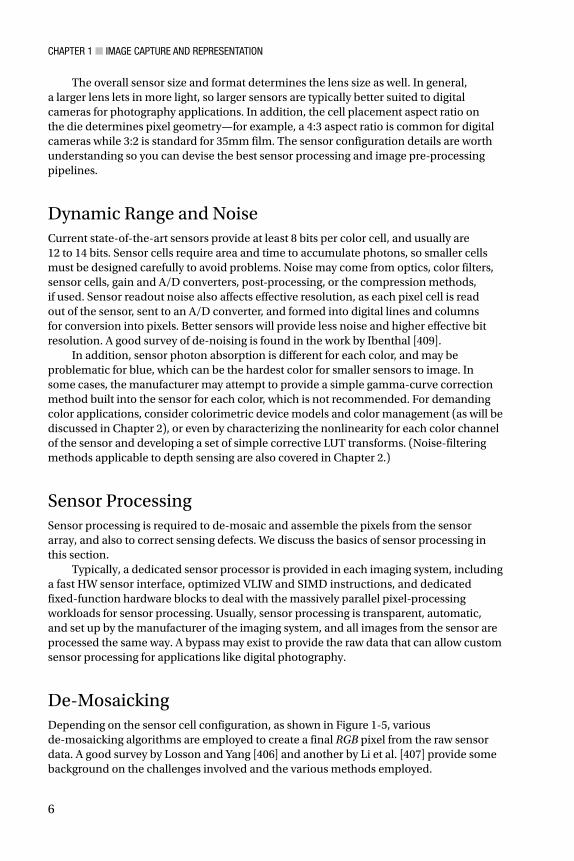
Dynamic Range and Noise Current state-of-the-art sensors provide at least 8 bits per color cell, and usually are 12 to 14 bits. Sensor cells require area and time to accumulate photons, so smaller cells must be designed carefully to avoid problems. Noise may come from optics, color filters, sensor cells, gain and A/D converters, post-processing, or the compression methods, if used. Sensor readout noise also affects effective resolution, as each pixel cell is read out of the sensor, sent to an A/D converter, and formed into digital lines and columns for conversion into pixels. Better sensors will provide less noise and higher effective bit resolution. A good survey of de-noising is found in the work by Ibenthal [409].

In addition, sensor photon absorption is different for each color, and may be problematic for blue, which can be the hardest color for smaller sensors to image. In some cases, the manufacturer may attempt to provide a simple gamma-curve correction method built into the sensor for each color, which is not recommended. For demanding color applications, consider colorimetric device models and color management (as will be discussed in Chapter 2), or even by characterizing the nonlinearity for each color channel of the sensor and developing a set of simple corrective LUT transforms. (Noise-filtering methods applicable to depth sensing are also covered in Chapter 2.)

Sensor Processing Sensor processing is required to de-mosaic and assemble the pixels from the sensor array, and also to correct sensing defects. We discuss the basics of sensor processing in this section.

Typically, a dedicated sensor processor is provided in each imaging system, including a fast HW sensor interface, optimized VLIW and SIMD instructions, and dedicated fixed-function hardware blocks to deal with the massively parallel pixel-processing workloads for sensor processing. Usually, sensor processing is transparent, automatic, and set up by the manufacturer of the imaging system, and all images from the sensor are processed the same way. A bypass may exist to provide the raw data that can allow custom sensor processing for applications like digital photography.

De-Mosaicking Depending on the sensor cell configuration, as shown in Figure 1-5 , various de-mosaicking algorithms are employed to create a final RGB pixel from the raw sensor data. A good survey by Losson and Yang [406] and another by Li et al. [407] provide some background on the challenges involved and the various methods employed.


7

One of the central challenges of de-mosaicking is pixel interpolation to combine the color channels from nearby cells into a single pixel. Given the geometry of sensor cell placement and the aspect ratio of the cell layout, this is not a trivial problem. A related issue is color cell weighting — for example, how much of each color should be integrated into each RGB pixel. Since the spatial cell resolution in a mosaicked sensor is greater than the final combined RGB pixel resolution, some applications require the raw sensor data to take advantage of all the accuracy and resolution possible, or to perform special processing to either increase the effective pixel resolution or do a better job of spatially accurate color processing and de-mosaicking.

Dead Pixel Correction A sensor, like an LCD display, may have dead pixels. A vendor may calibrate the sensor at the factory and provide a sensor defect map for the known defects, providing coordinates of those dead pixels for use in corrections in the camera module or driver software. In some cases, adaptive defect correction methods [408] are used on the sensor to monitor the adjacent pixels to actively look for defects and then to correct a range of defect types, such as single pixel defects, column or line defects, and defects such as 2x2 or 3x3 clusters. A camera driver can also provide adaptive defect analysis to look for flaws in real time, and perhaps provide special compensation controls in a camera setup menu.

Color and Lighting Corrections Color corrections are required to balance the overall color accuracy as well as the white balance. As shown in Figure 1-2 , color sensitivity is usually very good in silicon sensors for red and green, but less good for blue, so the opportunity for providing the most accurate color starts with understanding and calibrating the sensor.

Most image sensor processors contain a geometric processor for vignette correction, which manifests as darker illumination at the edges of the image, as shown in Chapter 7 (Figure 7-6). The corrections are based on a geometric warp function, which is calibrated at the factory to match the optics vignette pattern, allowing for a programmable illumination function to increase illumination toward the edges. For a discussion of image warping methods applicable to vignetting, see reference [490].

Geometric Corrections A lens may have geometric aberrations or may warp toward the edges, producing images with radial distortion, a problem that is related to the vignetting discussed above and shown in Chapter 7 (Figure 7-6). To deal with lens distortion, most imaging systems have a dedicated sensor processor with a hardware-accelerated digital warp unit similar to the texture sampler in a GPU. The geometric corrections are calibrated and programmed in the factory for the optics. See reference [490] for a discussion of image warping methods.


8

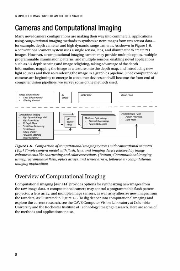
Cameras and Computational Imaging Many novel camera configurations are making their way into commercial applications using computational imaging methods to synthesize new images from raw sensor data—for example, depth cameras and high dynamic range cameras. As shown in Figure 1-6 , a conventional camera system uses a single sensor, lens, and illuminator to create 2D images. However, a computational imaging camera may provide multiple optics, multiple programmable illumination patterns, and multiple sensors, enabling novel applications such as 3D depth sensing and image relighting, taking advantage of the depth information, mapping the image as a texture onto the depth map, and introducing new light sources and then re-rendering the image in a graphics pipeline. Since computational cameras are beginning to emerge in consumer devices and will become the front end of computer vision pipelines, we survey some of the methods used.

Single Lens Single Flash

Programmable Flash - Pattern Projectors- Multi-Flash

Computational Imaging- High Dynamic Range HDR- High Frame Rates- 3D Depth Maps- Focal Plane Refocusing- Focal Sweep- Rolling Shutter- Panorama Stitching- Image Relighting

2D Sensor

2D SensorArray

Image Enhancements- Color Enhancements- Filtering, Contrast

Multi-lens Optics Arrays- Plenoptic Lens Arrays- Sphere/Ball Lenses

Figure 1-6. Comparison of computational imaging systems with conventional cameras . (Top) Simple camera model with flash, lens, and imaging device followed by image enhancements like sharpening and color corrections. (Bottom) Computational imaging using programmable flash, optics arrays, and sensor arrays, followed by computational imaging applications

Overview of Computational Imaging Computational imaging [447,414] provides options for synthesizing new images from the raw image data. A computational camera may control a programmable flash pattern projector, a lens array, and multiple image sensors, as well as synthesize new images from the raw data, as illustrated in Figure 1-6 . To dig deeper into computational imaging and explore the current research, see the CAVE Computer Vision Laboratory at Columbia University and the Rochester Institute of Technology Imaging Research. Here are some of the methods and applications in use.


9

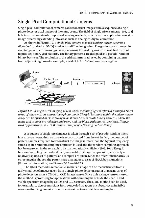
Single-Pixel Computational Cameras Single-pixel computational cameras can reconstruct images from a sequence of single photo detector pixel images of the same scene. The field of single-pixel cameras [103, 104] falls into the domain of compressed sensing research, which also has applications outside image processing extending into areas such as analog-to-digital conversion.

As shown in Figure 1-7 , a single-pixel camera may use a micro-mirror array or a digital mirror device (DMD), similar to a diffraction grating. The gratings are arranged in a rectangular micro-mirror grid array, allowing the grid regions to be switched on or off to produce binary grid patterns. The binary patterns are designed as a pseudo-random binary basis set. The resolution of the grid patterns is adjusted by combining patterns from adjacent regions—for example, a grid of 2x2 or 3x3 micro-mirror regions.

Figure 1-7. A single-pixel imaging system where incoming light is reflected through a DMD array of micro-mirrors onto a single photo-diode. The grid locations within the micro-mirror array can be opened or closed to light, as shown here, to create binary patterns, where the white grid squares are reflective and open, and the black grid squares are closed. (Image used by permission, © R. G. Baraniuk, Compressive Sensing Lecture Notes)

A sequence of single-pixel images is taken through a set of pseudo-random micro lens array patterns, then an image is reconstructed from the set. In fact, the number of pattern samples required to reconstruct the image is lower than the Nyquist frequency, since a sparse random sampling approach is used and the random sampling approach has been proven in the research to be mathematically sufficient [103, 104]. The grid basis-set sampling method is directly amenable to image compression, since only a relatively sparse set of patterns and samples are taken. Since the micro-mirror array uses rectangular shapes, the patterns are analogous to a set of HAAR basis functions. (For more information, see Figures 2-20 and 6-22.)

The DMD method is remarkable, in that an image can be reconstructed from a fairly small set of images taken from a single photo detector, rather than a 2D array of photo detectors as in a CMOS or CCD image sensor. Since only a single sensor is used, the method is promising for applications with wavelengths outside the near IR and visible spectrum imaged by CMOS and CCD sensors. The DMD method can be used, for example, to detect emissions from concealed weapons or substances at invisible wavelengths using non-silicon sensors sensitive to nonvisible wavelengths.


10

2D Computational Cameras Novel configurations of programmable 2D sensor arrays, lenses, and illuminators are being developed into camera systems as computational cameras [424,425,426], with applications ranging from digital photography to military and industrial uses, employing computational imaging methods to enhance the images after the fact. Computational cameras borrow many computational imaging methods from confocal imaging [419] and confocal microscopy [421, 420]—for example, using multiple illumination patterns and multiple focal plane images. They also draw on research from synthetic aperture radar systems [422] developed after World War II to create high-resolution images and 3D depth maps using wide baseline data from a single moving-camera platform. Synthetic apertures using multiple image sensors and optics for overlapping fields of view using wafer-scale integration are also topics of research [419]. We survey here a few computational 2D sensor methods, including high resolution (HR) , high dynamic range (HDR), and high frame rate (HF) cameras.

The current wave of commercial digital megapixel cameras, ranging from around 10 megapixels on up, provide resolution matching or exceeding high-end film used in a 35mm camera [412], so a pixel from an image sensor is comparable in size to a grain of silver on the best resolution film. On the surface, there appears to be little incentive to go for higher resolution for commercial use, since current digital methods have replaced most film applications and film printers already exceed the resolution of the human eye.

However, very high resolution gigapixel imaging devices are being devised and constructed as an array of image sensors and lenses, providing advantages for computational imaging after the image is taken. One configuration is the 2D array camera , composed of an orthogonal 2D array of image sensors and corresponding optics; another configuration is the spherical camera as shown in Figure 1-8 [411, 415], developed as a DARPA research project at Columbia University CAVE.


11

High dynamic range (HDR) cameras [416,417,418] can produce deeper pixels with higher bit resolution and better color channel resolution by taking multiple images of the scene bracketed with different exposure settings and then combining the images. This combination uses a suitable weighting scheme to produce a new image with deeper pixels of a higher bit depth, such as 32 pixels per color channel, providing images that go beyond the capabilities of common commercial CMOS and CCD sensors. HDR methods allow faint light and strong light to be imaged equally well, and can combine faint light and bright light using adaptive local methods to eliminate glare and create more uniform and pleasing image contrast.

Figure 1-8. (Top) Components of a very high resolution gigapixel camera, using a novel spherical lens and sensor arrangement.(Bottom) The resulting high-resolution images shown at 82,000 x 22,000 = 1.7 gigapixels. (All figures and images used by permission © Shree Nayar Columbia University CAVE research projects)


12

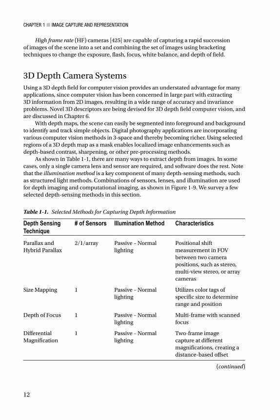
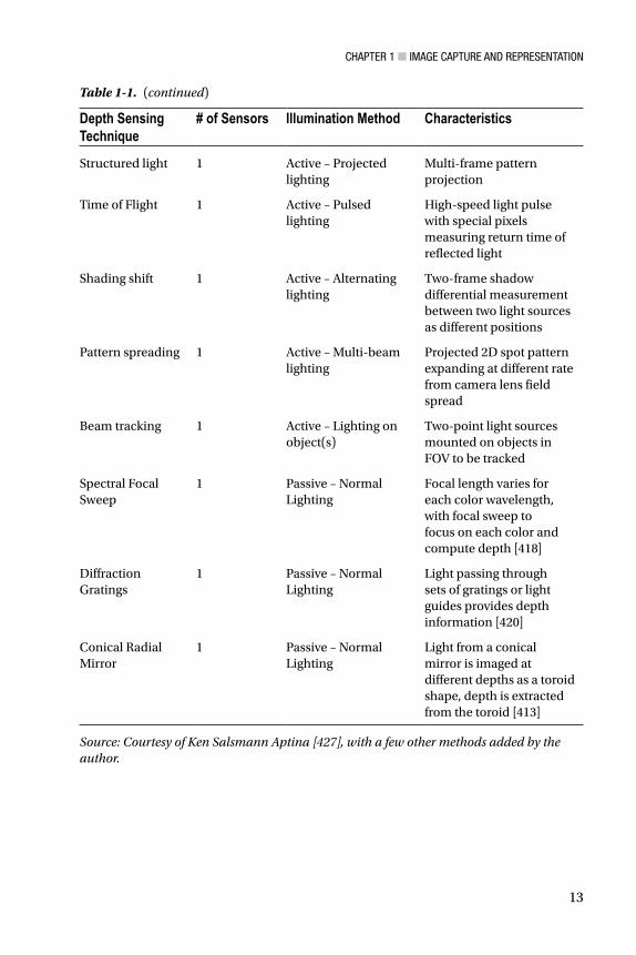
Table 1-1. Selected Methods for Capturing Depth Information

Depth Sensing Technique

# of Sensors Illumination Method Characteristics

Parallax and Hybrid Parallax

2/1/array Passive – Normal lighting

Positional shift measurement in FOV between two camera positions, such as stereo, multi-view stereo, or array cameras

Size Mapping 1 Passive – Normal lighting

Utilizes color tags of specific size to determine range and position

Depth of Focus 1 Passive – Normal lighting

Multi-frame with scanned focus

Differential Magnification

1 Passive – Normal lighting

Two-frame image capture at different magnifications, creating a distance-based offset

(continued)

High frame rate (HF) cameras [425] are capable of capturing a rapid succession of images of the scene into a set and combining the set of images using bracketing techniques to change the exposure, flash, focus, white balance, and depth of field.

3D Depth Camera Systems Using a 3D depth field for computer vision provides an understated advantage for many applications, since computer vision has been concerned in large part with extracting 3D information from 2D images, resulting in a wide range of accuracy and invariance problems. Novel 3D descriptors are being devised for 3D depth field computer vision, and are discussed in Chapter 6.

With depth maps, the scene can easily be segmented into foreground and background to identify and track simple objects. Digital photography applications are incorporating various computer vision methods in 3-space and thereby becoming richer. Using selected regions of a 3D depth map as a mask enables localized image enhancements such as depth-based contrast, sharpening, or other pre-processing methods.

As shown in Table 1-1 , there are many ways to extract depth from images. In some cases, only a single camera lens and sensor are required, and software does the rest. Note that the illumination method is a key component of many depth-sensing methods, such as structured light methods. Combinations of sensors, lenses, and illumination are used for depth imaging and computational imaging, as shown in Figure 1-9 . We survey a few selected depth-sensing methods in this section.


13

Depth Sensing Technique

# of Sensors Illumination Method Characteristics

Structured light 1 Active – Projected lighting

Multi-frame pattern projection

Time of Flight 1 Active – Pulsed lighting

High-speed light pulse with special pixels measuring return time of reflected light

Shading shift 1 Active – Alternating lighting

Two-frame shadow differential measurement between two light sources as different positions

Pattern spreading 1 Active – Multi-beam lighting

Projected 2D spot pattern expanding at different rate from camera lens field spread

Beam tracking 1 Active – Lighting on object(s)

Two-point light sources mounted on objects in FOV to be tracked

Spectral Focal Sweep

1 Passive – Normal Lighting

Focal length varies for each color wavelength, with focal sweep to focus on each color and compute depth [418]

Diffraction Gratings


Light passing through sets of gratings or light guides provides depth information [420]

Conical Radial Mirror


Light from a conical mirror is imaged at different depths as a toroid shape, depth is extracted from the toroid [413]

Source: Courtesy of Ken Salsmann Aptina [427], with a few other methods added by the author.

Table 1-1. (continued)


14

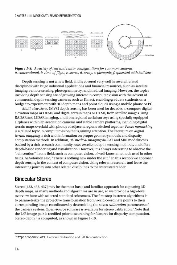
Depth sensing is not a new field, and is covered very well in several related disciplines with huge industrial applications and financial resources, such as satellite imaging, remote sensing, photogrammetry, and medical imaging. However, the topics involving depth sensing are of growing interest in computer vision with the advent of commercial depth-sensing cameras such as Kinect, enabling graduate students on a budget to experiment with 3D depth maps and point clouds using a mobile phone or PC.

Multi-view stereo (MVS) depth sensing has been used for decades to compute digital elevation maps or DEMs, and digital terrain maps or DTMs, from satellite images using RADAR and LIDAR imaging, and from regional aerial surveys using specially equipped airplanes with high-resolution cameras and stable camera platforms, including digital terrain maps overlaid with photos of adjacent regions stitched together. Photo mosaicking is a related topic in computer vision that’s gaining attention. The literature on digital terrain mapping is rich with information on proper geometry models and disparity computation methods. In addition, 3D medical imaging via CAT and MRI modalities is backed by a rich research community, uses excellent depth-sensing methods, and offers depth-based rendering and visualization. However, it is always interesting to observe the “reinvention” in one field, such as computer vision, of well-known methods used in other fields. As Solomon said, “There is nothing new under the sun.” In this section we approach depth sensing in the context of computer vision, citing relevant research, and leave the interesting journey into other related disciplines to the interested reader.

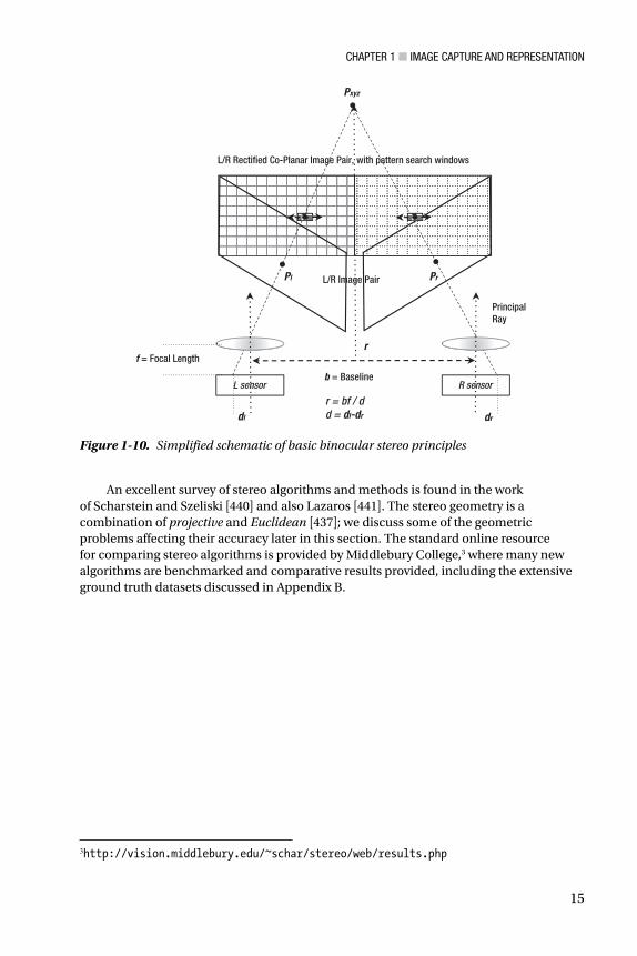
Binocular Stereo Stereo [432, 433, 437] may be the most basic and familiar approach for capturing 3D depth maps, as many methods and algorithms are in use, so we provide a high-level overview here with selected standard references. The first step in stereo algorithms is to parameterize the projective transformation from world coordinate points to their corresponding image coordinates by determining the stereo calibration parameters of the camera system. Open-source software is available for stereo calibration. 2 Note that the L/R image pair is rectified prior to searching for features for disparity computation. Stereo depth r is computed, as shown in Figure 1-10 .

RGB TOF1 2 3

4 5 6

7 8 9

LRGB

RRGB

Ball Lens

Lens Array

Sensor Array

RGB

a. b.

c.

d.

e.

f.

Figure 1-9. A variety of lens and sensor configurations for common cameras: a. conventional, b. time-of-flight, c. stereo, d. array, e. plenoptic, f. spherical with ball lens

2 http://opencv.org , Camera Calibration and 3D Reconstruction


15

Pxyz

b = Baseline

L/R Rectified Co-Planar Image Pair, with pattern search windows

L/R Image PairPl Pr

L sensor R sensor

Principal Ray

f = Focal Length

r = bf / dd = dl-dr

r

dl dr

Figure 1-10. Simplified schematic of basic binocular stereo principles

An excellent survey of stereo algorithms and methods is found in the work of Scharstein and Szeliski [440] and also Lazaros [441]. The stereo geometry is a combination of projective and Euclidean [437]; we discuss some of the geometric problems affecting their accuracy later in this section. The standard online resource for comparing stereo algorithms is provided by Middlebury College, 3 where many new algorithms are benchmarked and comparative results provided, including the extensive ground truth datasets discussed in Appendix B.

3 http://vision.middlebury.edu/~schar/stereo/web/results.php


16

The fundamental geometric calibration information needed for stereo depth includes the following basics.

• Camera Calibration Parameters. Camera calibration is outside the scope of this work, however the parameters are defined as 11 free parameters [435, 432]—3 for rotation, 3 for translation, and 5 intrinsic—plus one or more lens distortion parameters to reconstruct 3D points in world coordinates from the pixels in 2D camera space. The camera calibration may be performed using several methods, including a known calibration image pattern or one of many self-calibration methods [436]. Extrinsic parameters define the location of the camera in world coordinates, and intrinsic parameters define the relationships between pixel coordinates in camera image coordinates. Key variables include the calibrated baseline distance between two cameras at the principal point or center point of the image under the optics; the focal length of the optics; their pixel size and aspect ratio, which is computed from the sensor size divided by pixel resolution in each axis; and the position and orientation of the cameras.

• Fundamental Matrix or Essential Matrix. These two matrices are related, defining the popular geometry of the stereo camera system for projective reconstruction [438, 436, 437]. Their derivation is beyond the scope of this work. Either matrix may be used, depending on the algorithms employed. The essential matrix uses only the extrinsic camera parameters and camera coordinates, and the fundamental matrix depends on both the extrinsic and intrinsic parameters, and reveals pixel relationships between the stereo image pairs on epipolar lines.

In either case, we end up with projective transformations to reconstruct the 3D points from the 2D camera points in the stereo image pair.

Stereo processing steps are typically as follows:

1. Capture: Photograph the left/right image pair simultaneously.

2. Rectification: Rectify left/right image pair onto the same plane, so that pixel rows x coordinates and lines are aligned. Several projective warping methods may be used for rectification [437]. Rectification reduces the pattern match problem to a 1D search along the x -axis between images by aligning the images along the x -axis. Rectification may also include radial distortion corrections for the optics as a separate step; however, many cameras include a built-in factory-calibrated radial distortion correction.

3. Feature Description: For each pixel in the image pairs, isolate a small region surrounding each pixel as a target feature descriptor. Various methods are used for stereo feature description [215, 120].


17

4. Correspondence: Search for each target feature in the opposite image pair. The search operation is typically done twice, first searching for left-pair target features in the right image and then right-pair target features in the left image. Subpixel accuracy is required for correspondence to increase depth field accuracy.

5. Triangulation: Compute the disparity or distance between matched points using triangulation [439]. Sort all L/R target feature matches to find the best quality matches, using one of many methods [440].

6. Hole Filling: For pixels and associated target features with no corresponding good match, there is a hole in the depth map at that location. Holes may be caused by occlusion of the feature in either of the L/R image pairs, or simply by poor features to begin with. Holes are filled using local region nearest-neighbor pixel interpolation methods.

Stereo depth-range resolution is an exponential function of distance from the viewpoint: in general, the wider the baseline, the better the long-range depth resolution. A shorter baseline is better for close-range depth (see Figures 1-10 and 1-20 ). Human-eye baseline or inter-pupillary distance has been measured as between 50 and75mm, averaging about 70mm for males and 65mm for females.

Multi-view stereo (MVS) is a related method to compute depth from several views using different baselines of the same subject, such as from a single or monocular camera, or an array of cameras. Monocular, MVS, and array camera depth sensing are covered later in this section.

Structured and Coded Light Structured or coded light uses specific patterns projected into the scene and imaged back, then measured to determine depth; see Figure 1-11 . We define the following approaches for using structured light for this discussion [445]:

• Spatial single-pattern methods , requiring only a single illumination pattern in a single image.

• Timed multiplexing multi-pattern methods , requiring a sequence of pattern illuminations and images, typically using binary or n -array codes, sometimes involving phase shifting or dithering the patterns in subsequent frames to increase resolution. Common pattern sequences include gray codes, binary codes, sinusoidal codes, and other unique codes.


18

For example, in the original Microsoft Kinect 3D depth camera, structured light consisting of several slightly different micro-grid patterns or pseudo-random points of infrared light are projected into the scene, then a single image is taken to capture the spots as they appear in the scene. Based on analysis of actual systems and patent applications, the original Kinect computes the depth using several methods, including (1) the size of the infrared spot—larger dots and low blurring mean the location is nearer, while smaller dots and more blurring mean the location is farther away; (2) the shape of the spot—a circle indicates a parallel surface, an ellipse indicates an oblique surface; and (3) by using small regions or a micro pattern of spots together so that the resolution is not very fine—however, noise sensitivity is good. Depth is computed from a single image using this method, rather than requiring several sequential patterns and images.

Multi-image methods are used for structured light, including projecting sets of time-sequential structured and coded patterns, as shown in Figure 1-11 . In multi-image methods, each pattern is sent sequentially into the scene and imaged, then the combination of depth measurements from all the patterns is used to create the final depth map.

Industrial, scientific, and medical applications of depth measurements from structured light can reach high accuracy, imaging objects up to a few meters in size with precision that extends to micrometer range. Pattern projection methods are used, as well as laser-stripe pattern methods using multiple illumination beams to create wavelength interference; the interference is the measured to compute the distance. For example, common dental equipment uses small, hand-held laser range finders inserted into the mouth to create highly accurate depth images of tooth regions with missing pieces, and the images are then used to create new, practically perfectly fitting crowns or fillings using CAD/CAM micro-milling machines.

Of course, infrared light patterns do not work well outdoors in daylight; they become washed out by natural light. Also, the strength of the infrared emitters that can be used is limited by practicality and safety. The distance for effectively using structured light indoors is restricted by the amount of power that can be used for the IR emitters; perhaps

a.

b.

c. d.e.

f.

Figure 1-11. Selected structured light patterns and methods: a. gray codes, b. binary codes, c. regular spot grid, d. randomized spot grid (as used in original Kinect), e. sinusoidal phase shift patters, f. randomized pattern for compressive structured light [446]


19

5 meters is a realistic limit for indoor infrared light. Kinect claims a range of about 4 meters for the current TOF (time of flight) method using uniform constant infrared illumination, while the first-generation Kinect sensor had similar depth range using structured light.

In addition to creating depth maps, structured or coded light is used for measurements employing optical encoders, as in robotics and process control systems. The encoders measure radial or linear position. They provide IR illumination patterns and measure the response on a scale or reticle, which is useful for single-axis positioning devices like linear motors and rotary lead screws. For example, patterns such as the binary position code and the reflected binary gray code [444] can be converted easily into binary numbers (see Figure 1-11 ). The gray code set elements each have a Hamming distance of 1 between successive elements.

Structured light methods suffer problems when handling high-specular reflections and shadows; however, these problems can be mitigated by using an optical diffuser between the pattern projector and the scene using the diffuse structured light methods [443] designed to preserve illumination coding. In addition, multiple-pattern structured light methods cannot deal with fast-moving scenes; however, the single-pattern methods can deal well with frame motion, since only one frame is required.

Optical Coding: Diffraction Gratings Diffraction gratings are one of many methods of optical coding [447] to create a set of patterns for depth-field imaging, where a light structuring element, such as a mirror, grating, light guide, or special lens, is placed close to the detector or the lens. The original Kinect system is reported to use a diffraction grating method to create the randomized infrared spot illumination pattern. Diffraction gratings [430,431] above the sensor, as shown in Figure 1-12 , can provide angle-sensitive pixel sensing. In this case, the light is refracted into surrounding cells at various angles, as determined by the placement of the diffraction gratings or other beam-forming elements, such as light guides. This allows the same sensor data to be processed in different ways with respect to a given angle of view, yielding different images.

Photo-diodes

Gratings

Figure 1-12. Diffraction gratings above silicon used to create the Talbot Effect (first observed around 1836) for depth imaging. (For more information, see reference [430].) Diffraction gratings are a type of light-structuring element


20

This method allows the detector size to be reduced while providing higher resolution images using a combined series of low-resolution images captured in parallel from narrow aperture diffraction gratings. Diffraction gratings make it possible to produce a wide range of information from the same sensor data, including depth information, increased pixel resolution, perspective displacements, and focus on multiple focal planes after the image is taken. A diffraction grating is a type of illumination coding device.

As shown in Figure 1-13 , the light-structuring or coding element may be placed in several configurations, including [447]:

Object side coding: close to the subjects •

Pupil plane coding: close to the lens on the object side •

Focal plane coding: close to the detector •

Illumination coding: close to the illuminator •

DetectorDetector DetectorDetector

Optical Encoder +Illuminator

Optical Encoder Optical

Encoder

Optical Encoder

LensLensLensLens

Figure 1-13. Various methods for optical structuring and coding of patterns [447]: (Left to right): Object side coding, pupil plane coding, focal plane coding, illumination coding or structured light. The illumination patterns are determined in the optical encoder

Note that illumination coding is shown as structured light patterns in Figure 1-11 , while a variant of illumination coding is shown in Figure 1-7 , using a set of mirrors that are opened or closed to create patterns.

Time-of-Flight Sensors By measuring the amount of time taken for infrared light to travel and reflect, a time-of-flight (TOF) sensor is created [450]. A TOF sensor is a type of range finder or laser radar [449]. Several single-chip TOF sensor arrays and depth camera solutions are available, such as the second version of the Kinect depth camera. The basic concept involves broadcasting infrared light at a known time into the scene, such as by a pulsed IR laser, and then measuring the time taken for the light to return at each pixel. Sub-millimeter accuracy at ranges up to several hundred meters is reported for high-end systems [449], depending on the conditions under which the TOF sensor is used, the particular methods employed in the design, and the amount of power given to the IR laser.

Each pixel in the TOF sensor has several active components, as shown in Figure 1-14 , including the IR sensor well, timing logic to measure the round-trip time from illumination to detection of IR light, and optical gates for synchronization of the electronic shutter and the pulsed IR laser. TOF sensors provide laser range-finding


21

capabilities. For example, by gating the electronic shutter to eliminate short round-trip responses, environmental conditions such as fog or smoke reflections can be reduced. In addition, specific depth ranges, such as long ranges, can be measured by opening and closing the shutter at desired time intervals.

IR Sensor

Sensor Gate / Shutter

Pulsed IR Laser

Pulsed Light Gate

Timing controls

IR Illuminated scene

Figure 1-14. A hypothetical TOF sensor configuration. Note that the light pulse length and sensor can be gated together to target specific distance ranges

Illumination methods for TOF sensors may use very short IR laser pulses for a first image, acquire a second image with no laser pulse, and then take the difference between the images to eliminate ambient IR light contributions. By modulating the IR beam with an RF carrier signal using a photonic mixer device (PMD) , the phase shift of the returning IR signal can be measured to increase accuracy—which is common among many laser range-finding methods [450]. Rapid optical gating combined with intensified CCD sensors can be used to increase accuracy to the sub-millimeter range in limited conditions, even at ranges above 100 meters. However, multiple IR reflections can contribute errors to the range image, since a single IR pulse is sent out over the entire scene and may reflect off of several surfaces before being imaged.

Since the depth-sensing method of a TOF sensor is integrated with the sensor electronics, there is very low processing overhead required compared to stereo and other methods. However, the limitations of IR light for outdoor situations still remain [448], which can affect the depth accuracy.


22

Array Cameras As shown earlier in Figure 1-9 , an array camera contains several cameras, typically arranged in a 2D array, such as a 3x3 array, providing several key options for computational imaging. Commercial array cameras for portable devices are beginning to appear. They may use the multi-view stereo method to compute disparity, utilizing a combination of sensors in the array, as discussed earlier. Some of the key advantages of an array camera include a wide baseline image set to compute a 3D depth map that can see through and around occlusions, higher-resolution images interpolated from the lower-resolution images of each sensor, all-in-focus images, and specific image refocusing at one or more locations. The maximum aperture of an array camera is equal to the widest baseline between the sensors.

Radial Cameras A conical, or radial, mirror surrounding the lens and a 2D image sensor create a radial camera [413], which combines both 2D and 3D imaging. As shown in Figure 1-15 , the radial mirror allows a 2D image to form in the center of the sensor and a radial toroidal image containing reflected 3D information forms around the sensor perimeter. By processing the toroidal information into a point cloud based on the geometry of the conical mirror, the depth is extracted and the 2D information in the center of the image can be overlaid as a texture map for full 3D reconstruction.

Figure 1-15. (Left) Radial camera system with conical mirror to capture 3D reflections. (Center) Captured 3D reflections around the edges and 2D information of the face in the center. (Right) 3D image reconstructed from the radial image 3D information and the 2D face as a texture map. (Images used by permission © Shree Nayar Columbia University CAVE)


23

Plenoptics: Light Field Cameras Plenoptic methods create a 3D space defined as a light field, created by multiple optics. Plenoptic systems use a set of micro-optics and main optics to image a 4D light field and extract images from the light field during post-processing [451, 452, 423]. Plenoptic cameras require only a single image sensor, as shown in Figure 1-16 . The 4D light field contains information on each point in the space, and can be represented as a volume dataset, treating each point as a voxel, or 3D pixel with a 3D oriented surface, with color and opacity. Volume data can be processed to yield different views and perspective displacements, allowing focus at multiple focal planes after the image is taken. Slices of the volume can be taken to isolate perspectives and render 2D images. Rendering a light field can be done by using ray tracing and volume rendering methods [453, 454].

Subjects Main Lens SensorMicro-Lens Array

Figure 1-16. A plenoptic camera illustration. Multiple independent subjects in the scene can be processed from the same sensor image. Depth of field and focus can be computed for each subject independently after the image is taken, yielding perspective and focal plane adjustments within the 3D light field

In addition to volume and surface renderings of the light field, a 2D slice from the 3D field or volume can be processed in the frequency domain by way of the Fourier Projection Slice Theorem [455], as illustrated in Figure 1-17 . This is the basis for medical imaging methods in processing 3D MRI and CAT scan data. Applications of the Fourier Projection Slice method to volumetric and 3D range data are described by Levoy [455, 452] and Krig [137]. The basic algorithm is described as follows:

1. The volume data is forward transformed, using a 3D FFT into magnitude and phase data.

2. To visualize, the resulting 3D FFT results in the frequency volume are rearranged by octant shifting each cube to align the frequency 0 data around the center of a 3D Cartesian coordinate system in the center of the volume, similar to the way 2D frequency spectrums are quadrant shifted for frequency spectrum display around the center of a 2D Cartesian coordinate system.


24

3. A planar 2D slice is extracted from the volume parallel to the FOV plane where the slice passes through the origin (center) of the volume. The angle of the slice taken from the frequency domain volume data determines the angle of the desired 2D view and the depth of field.

4. The 2D slice from the frequency domain is run through an inverse 2D FFT to yield a 2D spatial image corresponding to the chosen angle and depth of field.

Figure 1-17. Graphic representation of the algorithm for the Fourier Projection Slice Theorem, which is one method of light field processing. The 3D Fourier space is used to filter the data to create 2D views and renderings [455, 452, 137]. (Image used by permission, © Intel Press, from Building Intelligent Systems)

3D Depth Processing For historical reasons, several terms with their acronyms are used in discussions of depth sensing and related methods, so we cover some overlapping topics in this section. Table 1-1 earlier provided a summary at a high level of the underlying physical means for depth sensing. Regardless of the depth-sensing method, there are many similarities and common problems. Post-processing the depth information is critical, considering the calibration accuracy of the camera system, the geometric model of the depth field, the measured accuracy of the depth data, any noise present in the depth data, and the intended application.

We survey several interrelated depth-sensing topics here, including:

Sparse depth-sensing methods •

Dense depth-sensing methods •

Optical flow •


25

Simultaneous localization and mapping (SLAM) •

Structure from motion (SFM) •

3D surface reconstruction , 3D surface fusion •

Monocular depth sensing •

Stereo and multi-view stereo (MVS) •

Common problems in depth sensing •

Human depth perception relies on a set of innate and learned visual cues, which are outside the scope of this work and overlap into several fields, including optics, ophthalmology, and psychology [464]; however, we provide an overview of the above selected topics in the context of depth processing.

Overview of Methods For this discussion of depth-processing methods, depth sensing falls into two major categories based on the methods shown in Table 1-1 :

• Sparse depth methods , using computer vision methods to extract local interest points and features. Only selected points are assembled into a sparse depth map or point cloud. The features are tracked from frame to frame as the camera or scene moves, and the sparse point cloud is updated. Usually only a single camera is needed.

• Dense depth methods , computing depth at every pixel. This creates a dense depth map, using methods such as stereo, TOF, or MVS. It may involve one or more cameras.

Many sparse depth methods use standard monocular cameras and computer vision feature tracking, such as optical flow and SLAM (which are covered later in this section), and the feature descriptors are tracked from frame to frame to compute disparity and sparse depth. Dense depth methods are usually based more on a specific depth camera technology, such as stereo or structured light. There are exceptions, as covered next.

Problems in Depth Sensing and Processing The depth-sensing methods each have specific problems; however, there are some common problems we can address here. To begin, one common problem is geometric modeling of the depth field, which is complex, including perspective and projections. Most depth-sensing methods treat the entire field as a Cartesian coordinate system, and this introduces slight problems into the depth solutions. A camera sensor is a 2D Euclidean model , and discrete voxels are imaged in 3D Euclidean space; however, mapping between the camera and the real world using simple Cartesian models introduces geometric distortion. Other problems include those of correspondence, or failure to match features in separate frames, and noise and occlusion . We look at such problems in this next section.


26

The Geometric Field and Distortions Field geometry is a complex area affecting both depth sensing and 2D imaging. For commercial applications, geometric field problems may not be significant, since locating faces, tracking simple objects, and augmenting reality are not demanding in terms of 3D accuracy. However, military and industrial applications often require high precision and accuracy, so careful geometry treatment is in order. To understand the geometric field problems common to depth-sensing methods, let’s break down the major areas:

Projective geometry problems, dealing with perspective •

Polar and spherical geometry problems, dealing with perspective • as the viewing frustum spreads with distance from the viewer

Radial distortion, due to lens aberrations •

Coordinate space problems, due to the Cartesian coordinates • of the sensor and the voxels, and the polar coordinate nature of casting rays from the scene into the sensor

The goal of this discussion is to enumerate the problems in depth sensing, not to solve them, and to provide references where applicable. Since the topic of geometry is vast, we can only provide a few examples here of better methods for modeling the depth field. It is hoped that, by identifying the geometric problems involved in depth sensing, additional attention will be given to this important topic. The complete geometric model, including corrections, for any depth system is very complex. Usually, the topic of advanced geometry is ignored in popular commercial applications; however, we can be sure that advanced military applications such as particle beam weapons and missile systems do not ignore those complexities, given the precision required.

Several researchers have investigated more robust nonlinear methods of dealing with projective geometry problems [465,466] specifically by modeling epipolar geometry–related distortion as 3D cylindrical distortion , rather than as planar distortion, and by providing reasonable compute methods for correction. In addition, the work of Lovegrove and Davison [484] deals with the geometric field using a spherical mosaicking method to align whole images for depth fusion, increasing the accuracy due to the spherical modeling.

The Horopter Region, Panum’s Area, and Depth Fusion

As shown in Figure 1-18 , the Horopter region, first investigated by Ptolemy and others in the context of astronomy, is a curved surface containing 3D points that are the same distance from the observer and at the same focal plane. Panum’s area is the region surrounding the Horopter where the human visual system fuses points in the retina into a single object at the same distance and focal plane. It is a small miracle that the human vision system can reconcile the distances between 3D points and synthesize a common depth field! The challenge with the Horopter region and Panum’s area lies in the fact that a post-processing step to any depth algorithm must be in place to correctly fuse the points the way the human visual system does. The margin of error depends on the usual variables, including baseline and pixel resolution, and the error is most pronounced


27

toward the boundaries of the depth field and less pronounced in the center. Some of the spherical distortion is due to lens aberrations toward the edges, and can be partially corrected as discussed earlier in this chapter regarding geometric corrections during early sensor processing.

Panum’s Area

Horopter

Fused depth points

Figure 1-18. Problems with stereo and multi-view stereo methods, showing the Horopter region and Panum’s area, and three points in space that appear to be the same point from the left eye’s perspective but different from the right eye’s perspective. The three points surround the Horopter in Panum’s area and are fused by humans to synthesize apparent depth

Cartesian vs. Polar Coordinates: Spherical Projective Geometry

As illustrated in Figure 1-19 , a 2D sensor as used in a TOF or monocular depth-sensing method has specific geometric problems as well; the problems increase toward the edges of the field of view. Note that the depth from a point in space to a pixel in the sensor is actually measured in a spherical coordinate system using polar coordinates, but the geometry of the sensor is purely Cartesian, so that geometry errors are baked into the cake .


28

Because stereo and MVS methods also use single 2D sensors, the same problems as affect single sensor depth-sensing methods also affect multi-camera methods, compounding the difficulties in developing a geometry model that is accurate and computationally reasonable.

Depth Granularity

As shown in Figure 1-20 , simple Cartesian depth computations cannot resolve the depth field into a linear uniform grain size; in fact, the depth field granularity increases exponentially with the distance from the sensor, while the ability to resolve depth at long ranges is much less accurate.

Sensor

P1 P2

P3

Figure 1-19. A 2D depth sensor and lens with exaggerated imaging geometry problems dealing with distance, where depth is different depending on the angle of incidence on the lens and sensor. Note that P

1 and P

2 are equidistant from the focal plane; however, the

distance of each point to the sensor via the optics is not equal, so computed depth will not be accurate depending on the geometric model used


29

For example, in a hypothetical stereo vision system with a baseline of 70mm using 480p video resolution, as shown in Figure 1-20 , depth resolution at 10 meters drops off to about ½ meter; in other words, at 10 meters away, objects may not appear to move in Z unless they move at least plus or minus ½ meter in Z . The depth resolution can be doubled simply by doubling the sensor resolution. As distance increases, humans increasingly use monocular depth cues to determine depth, such as for size of objects, rate of an object’s motion, color intensity, and surface texture details.

Correspondence Correspondence, or feature matching, is common to most depth-sensing methods. For a taxonomy of stereo feature matching algorithms, see Scharstein and Szeliski [440]. Here, we discuss correspondence along the lines of feature descriptor methods and triangulation as applied to stereo, multi-view stereo, and structured light.

Subpixel accuracy is a goal in most depth-sensing methods, so several algorithms exist [468]. It’s popular to correlate two patches or intensity templates by fitting the surfaces to find the highest match; however, Fourier methods are also used to correlate phase [467, 469], similar to the intensity correlation methods.

Y Pixel size: 480 / 10 meter = 20.8mmZy granularity = 465mm




Y Pixel size: 480 / 1 meter = 2mmZy granularity = 4mm

480p Sensor 480p Sensor

Stereo system, 480p sensors, 70mm baseline, 4.3mm focal lengthSensor Y die size = .672mmSensor Y Pixel size: .0014mmZy Granularity = ( .0014mm * Z2mm) / ( 4.3mm * 70mm)

Distance From Sensor in meters

Dept

h gr

anul

arity

or r

esol

utio

n in

mm

Dept

h gr

anul

arity

or r

esol

utio

n in

mm

Figure 1-20. Z depth granularity nonlinearity problems for a typical stereo camera system. Note that practical depth sensing using stereo and MVS methods has limitations in the depth field, mainly affected by pixel resolution, baseline, and focal length. At 10 meters, depth granularity is almost ½ meter, so an object must move at least + or- ½ meter in order for a change in measured stereo depth to be computed


30

For stereo systems, the image pairs are rectified prior to feature matching so that the features are expected to be found along the same line at about the same scale, as shown in Figure 1-11 ; descriptors with little or no rotational invariance are suitable [215, 120]. A feature descriptor such as a correlation template is fine, while a powerful method such as the SIFT feature description method [161] is overkill. The feature descriptor region may be a rectangle favoring disparity in the x -axis and expecting little variance in the y -axis, such as a rectangular 3x9 descriptor shape. The disparity is expected in the x -axis, not the y -axis. Several window sizing methods for the descriptor shape are used, including fixed size and adaptive size [440].

Multi-view stereo systems are similar to stereo; however, the rectification stage may not be as accurate, since motion between frames can include scaling, translation, and rotation. Since scale and rotation may have significant correspondence problems between frames, other approaches to feature description have been applied to MVS, with better results. A few notable feature descriptor methods applied to multi-view and wide baseline stereo include the MSER [194] method (also discussed in Chapter 6), which uses a blob-like patch, and the SUSAN [164, 165] method (also discussed in Chapter 6), which defines the feature based on an object region or segmentation with a known centroid or nucleus around which the feature exists.

For structured light systems, the type of light pattern will determine the feature, and correlation of the phase is a popular method [469]. For example, structured light methods that rely on phase-shift patterns using phase correlation [467] template matching claim to be accurate to 1/100 th of a pixel. Other methods are also used for structured light correspondence to achieve subpixel accuracy [467].

Holes and Occlusion

When a pattern cannot be matched between frames, a hole exists in the depth map. Holes can also be caused by occlusion. In either case, the depth map must be repaired, and several methods exist for doing that. A hole map should be provided, showing where the problems are. A simple approach, then, is to fill the hole uses use bi-linear interpolation within local depth map patches. Another simple approach is to use the last known-good depth value in the depth map from the current scan line.

More robust methods for handling occlusion exist [472, 471] using more computationally expensive but slightly more accurate methods, such as adaptive local windows to optimize the interpolation region. Yet another method of dealing with holes is surface fusion into a depth volume [473] (covered next), whereby multiple sequential depth maps are integrated into a depth volume as a cumulative surface, and then a depth map can be extracted from the depth volume.

Surface Reconstruction and Fusion

A general method of creating surfaces from depth map information is surface reconstruction. Computer graphics methods can be used for rendering and displaying the surfaces. The basic idea is to combine several depth maps to construct a better surface model, including the RGB 2D image of the surface rendered as a texture map . By creating an iterative model of the 3D surface that integrates several depth maps from


31

different viewpoints, the depth accuracy can be increased, occlusion can be reduced or eliminated, and a wider 3D scene viewpoint is created.

The work of Curless and Levoy [473] presents a method of fusing multiple range images or depth maps into a 3D volume structure. The algorithm renders all range images as iso-surfaces into the volume by integrating several range images. Using a signed distance function and weighting factors stored in the volume data structure for the existing surfaces, the new surfaces are integrated into the volume for a cumulative best-guess at where the actual surfaces exist. Of course, the resulting surface has several desirable properties, including reduced noise, reduced holes, reduced occlusion, multiple viewpoints, and better accuracy (see Figure 1-21 ).

b. TSDF or truncated signed distance function used to compute the zero-crossing at the estimated surface [473].

Raw Z depth map

RawYYZ vertex map & Surface normal map

6DOF pose via ICP

Volume surfaceintegration 3D surface rendering

Volume YYZ vertex map &Surface normal map

a. Method of volume integration, 6DOF camera pose, and surface rendering used in KinectFusion [474][475].

Figure 1-21. (Right) The Curless and Levoy [473] method for surface construction from range images, or depth maps. Shown here are three different weighted surface measurements projected into the volume using ray casting. (Left) Processing flow of Kinect Fusion method

A derivative of the Curless and Levoy method applied to SLAM is the Kinect Fusion approach [474], as shown in Figure 1-22 , using compute-intensive SIMD parallel real-time methods to provide not only surface reconstruction but also camera tracking and the 6DOF or 6-degrees-of-freedom camera pose. Raytracing and texture mapping are used for surface renderings. There are yet other methods for surface reconstruction from multiple images [480, 551].


32

Noise Noise is another problem with depth sensors [409], and various causes include low illumination and, in some cases, motion noise, as well as inferior depth sensing algorithms or systems. Also, the depth maps are often very fuzzy, so image pre-processing may be required, as discussed in Chapter 2, to reduce apparent noise. Many prefer the bi-lateral filter for depth map processing [302], since it respects local structure and preserves the edge transitions. In addition, other noise filters have been developed to remedy the weaknesses of the bi-lateral filter, which are well suited to removing depth noise, including the Guided Filter [486], which can perform edge-preserving noise filtering like the bi-lateral filter, the Edge-Avoiding Wavelet method [488], and the Domain Transform filter [489].

Monocular Depth Processing Monocular, or single sensor depth sensing, creates a depth map from pairs of image frames using the motion from frame to frame to create the stereo disparity. The assumptions for stereo processing with a calibrated fixed geometry between stereo pairs do not hold for monocular methods, since each time the camera moves the camera pose must be recomputed. Camera pose is a 6 degrees-of-freedom (6DOF) equation, including x, y, and z linear motion along each axis and roll, pitch, and yaw rotational motion about each axis. In monocular depth-sensing methods, the camera pose must be computed for each frame as the basis for comparing two frames and computing disparity.

Note that computation of the 6DOF matrix can be enhanced using inertial sensors, such as the accelerometer and MEMS gyroscope [483], as the coarse alignment step, followed by visual feature-based surface alignment methods discussed later in regard to optical flow . Since commodity inertial sensors are standard with mobile phones and tablets, inertial pose estimation will become more effective and commonplace as the sensors mature. While the accuracy of commodity accelerometers is not very good, monocular depth-sensing systems can save compute time by taking advantage of the inertial sensors for pose estimation.

Multi-View Stereo The geometry model for most monocular multi-view stereo (MVS) depth algorithms is based on projective geometry and epipolar geometry; a good overview of both are found in the classic text by Hartley and Zisserman [437]. A taxonomy and accuracy comparison of six MVS algorithms is provided by Seitz et al. [478]. We look at a few representative approaches in this section.

Iterative surface alignment solution over Image Pyramid

Figure 1-22. Graphic representaion of the dense whole-image alignment solution to obtain the 6DOF camera pose using ESM [485]


33

Sparse Methods: PTAM Sparse MVS methods create a sparse 3D point cloud, not a complete depth map. The basic goals for sparse depth are simple: track the features from frame to frame, compute feature disparity to create depth, and perform 6DOF alignment to localize the new frames and get the camera pose. Depending on the application, sparse depth may be ideal to use as part of a feature descriptor to add invariance to perspective viewpoint or to provide sufficient information for navigating that’s based on a few key landmarks in the scene. Several sparse depth-sensing methods have been developed in the robotics community under the terms SLAM , SFM , and optical flow (discussed below).

However, we first illustrate sparse depth sensing in more detail by discussing a specific approach: Parallel Tracking and Mapping (PTAM) [456, 457], which can both track the 6DOF camera pose and generate a sparse depth map suitable for light-duty augmented reality applications, allowing avatars to be placed at known locations and orientations in the scene from frame to frame. The basic algorithm consists of two parts, which run in parallel threads: a tracking thread for updating the pose, and a mapping thread for updating the sparse 3D point cloud. We provide a quick overview of each next.

The mapping thread deals with a history buffer of the last N keyframes and an N-level image pyramid for each frame in a history buffer, from which the sparse 3D point cloud is continually refined using the latest incoming depth features via a bundle adjustment process (which simply means fitting new 3D coordinates against existing 3D coordinates by a chosen minimization method, such as the Levenberg-Marquardt [437]). The bundle adjustment process can perform either a local adjustment over a limited set of recent frames or global adjustment over all the frames during times of low scene motion when time permits.

The tracking thread scans the incoming image frames for expected features, based on projecting where known-good features last appeared, to guide the feature search, using the 6DOF camera pose as a basis for the projection. A FAST9 [138] corner detector is used to locate the corners, followed by a Shi-Tomasi [157] non-maximal suppression step to remove weak corner candidates (discussed in Chapter 6 in more detail). The feature matching stage follows a coarse-to-fine progression over the image pyramid to compute the 6DOF pose.

Target features are computed in new frames using an 8x8 patch surrounding each selected corner. Reference features are computed also as 8x8 patches from the original patch taken from the first-known image where they were found. To align the reference and target patches prior to feature matching, the surface normal of each reference patch is used for pre-warping the patch against the last-known 6DOF camera pose, and the aligned feature matching is performed using zero-mean SSD distance.

One weakness of monocular depth sensing shows up when there is a failure to localize ; that is, if there is too much motion, or illumination changes too much, the system may fail to localize and the tracking stops. Another weakness is that the algorithm must be initialized entirely for a specific localized scene or workspace, such as a desktop. For initialization, PTAM follows a five-point stereo calibration method that takes a few seconds to perform with user cooperation. Yet another weakness is that the size of the 3D volume containing the point cloud is intended for a small, localized scene or workspace. However, on the positive side, the accuracy of the 3D point cloud is very good, close to the pixel size; the pose is accurate enough for AR or gaming applications; and it is possible to


34

create a 360-degree perspective point cloud by walking around the scene. PTAM has been implemented on a mobile phone [456] using modest compute and memory resources, with tradeoffs for accuracy and frame rate.

Dense Methods: DTAM Dense monocular depth sensing is quite compute-intensive compared to sparse methods, so the research and development are much more limited. The goals are about the same as for sparse monocular depth—namely, compute the 6DOF camera pose for image alignment, but create a dense every-pixel depth map instead of a sparse point cloud. For illustration, we highlight key concepts from a method for Dense Tracking and Mapping (DTAM) , developed by Newcombe, Lovegrove and Davison [482].

While the DTAM goal is to compute dense depth at each pixel rather than sparse depth, DTAM shares some of the same requirements with PTAM [457], since both are monocular methods. Both DTAM and PTAM are required to compute the 6DOF pose for each new frame in order to align the new frames to compute disparity. DTAM also requires a user-assisted monocular calibration method for the scene, and it uses the PTAM calibration method. And DTAM is also intended for small, localized scenes or workspaces. DTAM shares several background concepts taken from the Spherical Mosaicking method of Lovegrove and Davison [484], including the concept of whole image alignment, based on the Efficient Second Order Minimization (ESM) method [485], which is reported to find a stable surface alignment using fewer iterations than LK methods [458] as part of the process to generate the 6DOF pose.

Apparently, both DTAM and Spherical Mosaicking use a spherical coordinate geometry model to mosaic the new frames into the dense 3D surface proceeding from coarse to fine alignment over the image pyramid to iterate toward the solution of the 6DOF camera pose. The idea of whole-image surface alignment is shown in Figure 1-22 . The new and existing depth surfaces are integrated using a localized guided-filter method [486] into the cost volume. That is, the guided filter uses a guidance image to merge the incoming depth information into the cost volume.

DTAM also takes great advantage of SIMD instructions and highly thread-parallel SIMT GPGPU programming to gain the required performance necessary for real-time operation on commodity GPU hardware.

Optical Flow, SLAM, and SFM Optical flow measures the motion of features and patterns from frame to frame in the form of a displacement vector . Optical flow is similar to sparse monocular depth-sensing methods, and it can be applied to wide baseline stereo matching problems [463]. Since the field of optical flow research and its applications is vast [459, 460, 461], we provide only an introduction here with an eye toward describing the methods used and features obtained.

Optical flow can be considered a sparse feature-tracking problem, where a feature can be considered a particle [462], so optical flow and particle flow analysis are similar. Particle flow analysis is applied to diverse particle field flow-analysis problems, including


35

weather prediction, simulating combustion and explosives, hydro-flow dynamics, and robot navigation. Methods exist for both 2D and 3D optical flow. The various optical flow algorithms are concerned with tracking-feature descriptors or matrices, rather than with individual scalars or pixels, within consecutive fields of discrete scalar values. For computer vision, the input to the optical flow algorithms is a set of sequential 2D images and pixels, or 3D volumes and voxels, and the output is a set of vectors showing direction of movement of the tracked features.

Many derivations and alternatives to the early Lucas Kanade (LK) method [458, 459, 460, 461] are used for optical flow; however, this remains the most popular reference point, as it uses local features in the form of correlation templates (as discussed in Chapter 6). Good coverage of the state-of-the-art methods based on LK is found in Lucas Kanade 20 years on, by Baker and Matthews [480]. The Efficient Second Order Minimization (ESM) method [485] is related to the LK method. ESM is reported to be a stable solution using fewer iterations than LK. LK does not track individual pixels; rather, it relies on the pixel neighborhood, such as a 3x3 matrix or template region, and tries to guess which direction the features have moved, iteratively searching the local region and averaging the search results using a least-squares solution to find the best guess.

While there are many variations on the LK method [459, 460, 461], key assumptions of most LK-derived optical flow methods include small displacements of features from frame to frame, rigid features, and sufficient texture information in the form of localized gradients in order to identify features. Various methods are used to find the local gradients, such as Sobel and Laplacian (discussed in Chapter 2). Fields with large feature displacements from frame to frame and little texture information are not well suited to the LK method. That’s because the LK algorithm ignores regions with little gradient information by examining the eigenvalues of each local matrix to optimize the iterative solution. However, more recent and robust research methods are moving beyond the limitations of LK [459,460], and include Deepflow [344], which is designed for deformable features and large displacement optical flow [394], using multi-layer feature scale hierarchies [404] similar to convolutional networks [339].

Applications of surface reconstruction to localization and mapping are used in simultaneous localization and mapping (SLAM ) and instructure from motion (SFM) methods—for example, in robotics navigation. One goal of SLAM is to localize, or find the current position and the 6DOF camera pose. Another goal is to create a local region map, which includes depth. To dig deeper into SLAM and SFM methods, see the historical survey by Bailey and Hugh Durrant-Whyte [476, 477].

3D Representations : Voxels, Depth Maps, Meshes, and Point Clouds Depth information is represented and stored in a variety of convertible formats, depending on the intended use. We summarize here some common formats; see also Figure 1-23 .


36

The ability to convert between depth formats is desirable for different algorithms and easy to do. Common 3D depth formats include:

• 2D Pixel Array, 3D Depth Map: A 2D pixel array is the default format for 2D images in memory, and it is the natural storage format for many processing operations, such as convolution and neighborhood filtering. For depth map images, the pixel value is the Z , or depth value. Each point in the array may contain {color, depth}.

• 3D Voxel Volume: A 3D volumetric data structure composed of a 3D array of voxels is ideal for several algorithms, including depth map integration for 3D surface reconstruction and raytracing of surfaces for graphical renderings. A voxel is a volume element, like a pixel is a picture element. Each voxel may contain {color, normal} ; the depth coordinates are implicit from the volume structure.

• 3D Polygon Mesh: Storing 3D points in a standard 3D polygon mesh provides a set of connected points or vertices, each having a surface normal, 3D coordinates, color, and texture. Mesh formats are ideal for rendering surfaces in a GPU pipeline, such as OpenGL or DirectX. Each point in the mesh may contain {x, y, z, color, normal}, and is associated with neighboring points in a standard pattern such as a quad or triangle describing the surface.

• 3D Point Cloud: This is a sparse structure that is directly convertible to a standard 3D polygon mesh. The point cloud format is ideal for sparse monocular depth-sensing methods. Each point in the cloud may contain {x, y, z, color, normal}.

Figure 1-23. Various 3D depth formats. Renderings of a Zernike polynomial. (Left to right): A depth map, a polygon mesh rendering using 3D quads, a point cloud rendering equivalent of voxels


37

Summary In this chapter, we surveyed image sensing methods and sensor image processing methods as the first step in the vision pipeline. We covered the image sensor technologies available, with an eye toward image pre-processing that may be useful for getting the most from the image data, since image sensoring methods often dictate the image pre-processing required. (More discussion on image pre-processing is provided in Chapter 2.) Sensor configurations used for both 2D and 3D imaging were discussed, as well as a wide range of camera configurations used for computational imaging to create new images after the data is captured, such as HDR images and image refocusing. Depth imaging approaches were covered here as well, and included stereo and time of flight, since mobile devices are increasingly offering 3D depth camera technology for consumer applications. Depth maps can be used in computer vision to solve many problems, such as 3D feature description and 3D image segmentation of foreground and background objects. The topic of 3D depth processing and 3D features is followed throughout this book; chapter 6 covers 3D feature descriptors, and chapter 7 and Appendix B cover 3D ground truth data.

Image Capture and Representation€¦ · Image Capture and Representation “The changing of bodies...

Documents

Transcript of Image Capture and Representation€¦ · Image Capture and Representation “The changing of bodies...