Image Acquisition and Processing With LabVIEW
268
-
Upload
prakash-nayak -
Category
Documents
-
view
54 -
download
2
Transcript of Image Acquisition and Processing With LabVIEW


IMAGE PROCESSING SERIESSeries Editor: Phillip A. Laplante, Pennsylvania Institute of Technology
Published Titles
Adaptive Image Processing: A Computational Intelligence PerspectiveStuart William Perry, Hau-San Wong, and Ling Guan
Image Acquisition and Processing with LabVIEW™
Christopher G. Relf
Image and Video Compression for Multimedia EngineeringYun Q. Shi and Huiyang Sun
Multimedia Image and Video ProcessingLing Guan, S.Y. Kung, and Jan Larsen
Shape Analysis and Classification: Theory and PracticeLuciano da Fontoura Costa and Roberto Marcondes Cesar Jr.
Software Engineering for Image Processing SystemsPhillip A. Laplante


1480_book.fm Page 4 Tuesday, June 24, 2003 11:35 AM
This book contains information obtained from authentic and highly regarded sources. Reprinted materialis quoted with permission, and sources are indicated. A wide variety of references are listed. Reasonableefforts have been made to publish reliable data and information, but the author and the publisher cannotassume responsibility for the validity of all materials or for the consequences of their use.
Neither this book nor any part may be reproduced or transmitted in any form or by any means, electronicor mechanical, including photocopying, microÞlming, and recording, or by any information storage orretrieval system, without prior permission in writing from the publisher.
The consent of CRC Press LLC does not extend to copying for general distribution, for promotion, forcreating new works, or for resale. SpeciÞc permission must be obtained in writing from CRC Press LLCfor such copying.
Direct all inquiries to CRC Press LLC, 2000 N.W. Corporate Blvd., Boca Raton, Florida 33431.
Trademark Notice: Product or corporate names may be trademarks or registered trademarks, and areused only for identiÞcation and explanation, without intent to infringe.
Visit the CRC Press Web site at www.crcpress.com
© 2004 by CRC Press LLC
No claim to original U.S. Government worksInternational Standard Book Number 0-8493-1480-1
Library of Congress Card Number 2003046135Printed in the United States of America 1 2 3 4 5 6 7 8 9 0
Printed on acid-free paper
Library of Congress Cataloging-in-Publication Data
Relf, Christopher G.Image acquisition and processing with LabVIEW / Christopher G. Relf
p. cm. (Image processing series)Includes bibliographical references and index.ISBN 0-8493-1480-11. Image processing--Digital techniques. 2. Engineering instruments--Data processing. 3.LabVIEW. I. Title. II. Series.
TA1632.R44 2003621.36�7�dc21 2003046135
CIP

1480_book.fm Page 5 Tuesday, June 24, 2003 11:35 AM
Foreword
The introduction of LabVIEW over 16 years ago triggered the Virtual Instrumenta-tion revolution that is still growing rapidly today. The tremendous advances inpersonal computers and consumer electronics continue to fuel this growth. For thesame cost, today�s computers are about 100 times better than the machines of theLabVIEW 1 days, in CPU clock rate, RAM size, bus speed and disk size. Thistrend will likely continue for another 5 to 10 years.
Virtual Instrumentation Þrst brought the connection of electronic instruments tocomputers, then later added the ability to plug measurement devices directly intothe computer. Then, almost 7 years ago, National Instruments expanded the visionof virtual instrumentation when it introduced its Þrst image acquisition hardwarealong with the LabVIEW Image Analysis library. At the time, image processing ona personal computer was still a novelty requiring the most powerful machines anda lot of specialized knowledge on the part of the system developer. Since then,computer performance and memory size have continued to increase to the pointwhere image processing is now practical on most modern PCs. In addition, the rangeof product offerings has expanded and higher-level software, such as Vision Builder,has become available to make development of image processing applications mucheasier.
Today, image processing is fast becoming a mainstream component of VirtualInstrumentation. Very few engineers, however, have had experience with imageprocessing or the lighting techniques required to capture images that can be pro-cessed quickly and accurately. Hence the need for a book like this one. ChristopherRelf has written a very readable and enjoyable introduction to image processing,with clear and straightforward examples to illustrate the concepts, good referencesto more detailed information, and many real-world solutions to show the breadth ofvision applications that are possible. The lucid (pun intended) description of the roleof, and options for, lighting is itself worth the price of the book.
Jeff KodoskyNational Instruments Fellow
Co-inventor of LabView

1480_book.fm Page 6 Tuesday, June 24, 2003 11:35 AM

1480_book.fm Page 7 Tuesday, June 24, 2003 11:35 AM
Preface
Image Acquisition and Processing with LabVIEW Þlls a hole in the LabVIEWtechnical publication range. It is intended for competent LabVIEW programmers,as a general training manual for those new to National Instruments� (NI) Visionapplication development and a reference for more-experienced vision programmers.It is assumed that readers have attained programming knowledge comparable to thattaught in the NI LabVIEW Basics II course (see http://www.ni.com/training for adetailed course outline). The book covers introductions and theory of general imageacquisition and processing topics, while providing more in-depth discussions andexamples of speciÞc NI Vision tools.
This book is a comprehensive IMAQ and Vision resource combining referencematerial, theory on image processing techniques, information on how LabVIEW andthe NI Vision toolkit handle each technique, examples of each of their uses and real-world case studies, all in one book.
This is not a �laboratory-style� book, and hence does not contain exercises forthe reader to complete. Instead, the several coding examples, as referenced in thetext, are included on an accompanying CD-ROM in the back of the book.
The information contained in this book refers generally to the National Instru-ments Vision Toolkit version 6.1 (Figure 1). Several of the techniques explained hereinmay be perfectly functional using previous or future versions of the Vision Toolkit
A glossary has also been compiled to deÞne subject-related words and acronyms.
THE COMPANION CD-ROM
Like most modern computer-related technical books, this one is accompaniedby a companion CD-ROM that contains libraries of example images and code, asreferenced in the text. Every wiring diagram shown in this book has correspondingsource code on the CD-ROM for your convenience � just look in the respectivechapter�s folder for a Þle with the same name as the image�s caption (Figure 2).
To use the code, you will need:
� LabVIEW 6.1 (or higher)� LabVIEW Vision Toolkit 6.1 (or higher)� An operating system that supports both of these components
Some of the examples may also require the following components to be installed:
� IMAQ� Vision Builder 6.1 (or higher)� IMAQ OCR Toolkit� IMAQ 1394 Drivers

1480_book.fm Page 8 Tuesday, June 24, 2003 11:35 AM
The CD-ROM also contains all of the example images used to test the codefeatured in the book, a demonstration version of National Instruments LabVIEW6.0, and a National Instruments IMAQ Demonstration that guides you through someof the features of NI-IMAQ.
FIGURE 1 Vision 6.1
FIGURE 2 Companion CD-ROM Contents

1480_book.fm Page 9 Tuesday, June 24, 2003 11:35 AM
Author
Christopher G. Relf is an Industrial Automation SoftwareEngineering consultant and LabVIEW specialist. Previously,his work at JDS Uniphase Pty Ltd (www.jdsu.com) includedthe automation of several complex processes, including thelaser writing of optical FBGs (Fiber Bragg Gratings) andtheir measurement. Mr. Relf was part of a strong LabVIEWteam that designed and implemented a plug-in-style softwaresuite that introduced an �any product, any process, any-where� paradigm to both the production and R&D phasesof product creation. As a Computational Automation Scien-tist with the Division of Telecommunications and IndustrialPhysics, CSIRO, (www.tip.csiro.au), Australia�s premier sci-entiÞc and industrial research organization, he was the prin-cipal software engineer of several projects including theautomation of thin Þlm Þltered arc deposition and metal shell
eccentricity systems. He has consulted to the New South Wales Institute of Sport(www.nswis.com.au) and provided advice on the development of automated sportscience data acquisition systems, used to test and train some of Australia�s premierathletes.
Mr. Relf completed his undergraduate science degree in applied physics at theUniversity of Technology, Sydney, where he Þrst learned the virtues of LabVIEWversion 3, and has been a strong G programming advocate ever since. He gained hisCertiÞed LabVIEW Developer qualiÞcation from National Instruments in 2002.
Mr. Relf can be contacted via e-mail at [email protected]

1480_book.fm Page 10 Tuesday, June 24, 2003 11:35 AM

1480_book.fm Page 11 Tuesday, June 24, 2003 11:35 AM
Acknowledgments
My gratitude goes out to all of the people at CRC Press LLC who have held myhand through the production of this book. SpeciÞcally, thanks to Nora Konopka, myAcquisitions Editor, who showed immense faith in taking on and internally promot-ing this project; Helena Redshaw, my Editorial Project Development Supervisor,who kept me on the right track during the book�s development; and Sylvia Wood,my Project Editor, who worked closely with me to convert my ramblings intocomprehensible format.
The user solutions featured were written by some very talented LabVIEW andVision specialists from around the world, most of whom I found lurking either onthe Info-LabVIEW Mailing List (http://www.info-labview.org), or the NI-Zone Dis-cussion Forum (http://www.zone.ni.com). Theoretical descriptions of the Visioncapabilities of LabVIEW are all very well, but it is only when you build a programthat ties the individual functionalities together to form a useful application that yourealize the true value of their use. I hope their stories help you to see the big picture(pun intended), and to realize that complete solutions can be created around coreVision components. Thank you for the stories and examples showing some of thereal-world applications achievable using the techniques covered in the book.
A big thank you goes out to my two very talented reviewers, Edward Lipnickiand Peter Badcock, whose knowledge of theory often overshadowed my scientiÞcassumptions � this book would not be anywhere near as comprehensive withoutyour help. Thanks also to my proofreaders, Adam Batten, Paul Conroy, ArchieGarcia, Walter Kalceff, James McDonald, Andrew Parkinson, Paul Relf, AnthonyRochford, Nestor Sanchez, Gil Smith, Glen Trudgett and Michael Wallace, whohelped me correct most (hopefully) of the mistakes I made in initial manuscripts.
The section on application lighting is based primarily on information and imagesI gathered from NER (a Robotic Vision Systems Incorporated company) � thankyou to Greg Dwyer from the Marketing Communications group for assisting me inputting it all together. Further information regarding NER�s extensive range ofindustrial lighting products can be found at their Web site (http://www.nerlite.com).
I could not have dreamed of writing this book without the assistance of my localNational Instruments staff, Jeremy Carter (Australia and New Zealand Branch Man-ager) and Alex Gouliaev (Field Sales Engineer). Your product-related assistance anddepth of knowledge of NI products and related technologies were invaluable andnowhere short of astounding.
My apologies to my family, my friends and all of my English teachers. Thisbook is pitched primarily to readers in the United States, so I have had to abandonmany of the strict rules of English spelling and grammar that you tried so hard toinstill in me. I hope that you can forgive me.

1480_book.fm Page 12 Tuesday, June 24, 2003 11:35 AM
Thanks must also go to Ed, Gleno, Jase, Rocko and Adrian, who were alwaysmore than willing to help me relax with a few schooners between (and occasionallyduring) chapters.
Those who have written a similar-level technical book understand the drainingexercise that it is, and my love and humble appreciation go to my family and friends,who supported me in many ways through this project. Ma and Paul, who plantedthe �you-can-do-anything� seed, and Ruth, who tends the resulting tree every day:I couldn�t have done it without you all.
Christopher G. Relf

1480_book.fm Page 13 Tuesday, June 24, 2003 11:35 AM
Dedication
To Don �old fella� Price. I appreciate your inspiration, support, friendship
and, above all else, your good humor.

1480_book.fm Page 14 Tuesday, June 24, 2003 11:35 AM

1480_book.fm Page 15 Tuesday, June 24, 2003 11:35 AM
Introduction
Of the Þve senses we use daily, we rely most on our sense of sight. Our eyesightprovides 80% of the information we absorb during daylight hours, and it is nowonder, as nearly three quarters of the sensory receptor cells in our bodies are locatedin the back of our eyes, at the retinas. Many of the decisions we make daily arebased on what we can see, and how we in turn interpret that data � an action ascommon as driving a car is only possible for those who have eyesight.
As computer-controlled robotics play an ever-increasing role in factory produc-tion, scientiÞc, medical and safety Þelds, surely one of the most important andintuitive advancements we can exploit is the ability to acquire, process and makedecisions based on image data.
LabVIEW is a popular measurement and automation programming language,developed by National Instruments (NI). Initially aimed squarely at scientists andtechnicians to assist in simple laboratory automation and data acquisition, LabVIEWhas grown steadily to become a complete programming language in its own right,with add-on toolkits that cover anything from Internet connectivity and databaseaccess to fuzzy logic and image processing. The image-based toolkit (called Vision)is particularly popular, simplifying the often-complex task of not only downloadingappropriate quality images into a computer, but also making multifarious processingtasks much easier than many other packages and languages.
This book is intended for competent LabVIEW programmers, as a generaltraining manual for those new to NI Vision application development and a referencefor more-experienced Vision programmers. It is assumed that you have attainedprogramming knowledge comparable to that taught in the NI LabVIEW Basics IIcourse.
I sincerely hope that you will learn much from this book, that it will aid you indeveloping and including Vision components conÞdently in your applications, thusharnessing one of the most complex, yet common data sources � the photon.

1480_book.fm Page 16 Tuesday, June 24, 2003 11:35 AM

1480_bookTOC.fm Page 23 Tuesday, June 24, 2003 4:38 PM
Contents
Chapter 1 Image Types and File Management.....................................................1
1.1 Types of Images ...............................................................................................11.1.1 Grayscale ..............................................................................................21.1.2 Color.....................................................................................................31.1.3 Complex ...............................................................................................4
1.2 File Types .........................................................................................................41.2.1 Modern File Formats ...........................................................................5
1.2.1.1 JPEG .....................................................................................71.2.1.2 TIFF ......................................................................................71.2.1.3 GIF ........................................................................................71.2.1.4 PNG.......................................................................................81.2.1.5 BMP ......................................................................................81.2.1.6 AIPD .....................................................................................81.2.1.7 Other Types...........................................................................8
1.3 Working with Image Files ...............................................................................91.3.1 Standard Image Files ...........................................................................91.3.2 Custom and Other Image Formats.....................................................12
Chapter 2 Setting Up ..........................................................................................15
2.1 Cameras ..........................................................................................................152.1.1 Scan Types .........................................................................................16
2.1.1.1 Progressive Area Scan ........................................................162.1.1.2 Interlaced Area Scan...........................................................162.1.1.3 Interlacing Standards ..........................................................172.1.1.4 Line Scan ............................................................................182.1.1.5 Camera Link .......................................................................192.1.1.6 Thermal ...............................................................................20
2.1.2 Camera Advisors: Web-Based Resources..........................................202.1.3 User Solution: X-Ray Inspection System..........................................22
2.1.3.1 Introduction.........................................................................222.1.3.2 Control and Imaging Hardware Configuration ..................232.1.3.3 Control Software.................................................................232.1.3.4 Imaging Software................................................................242.1.3.5 Conclusions.........................................................................25
2.2 Image Acquisition Hardware .........................................................................262.2.1 National Instruments Frame Grabbers...............................................26

1480_bookTOC.fm Page 24 Tuesday, June 24, 2003 4:38 PM
2.2.2 IEEE 1394 (FireWire) Systems .........................................................262.2.3 USB Systems......................................................................................29
2.3 From Object to Camera .................................................................................302.3.1 Resolution...........................................................................................302.3.2 Depth of Field (DOF) ........................................................................312.3.3 Contrast (or Modulation) ...................................................................322.3.4 Perspective (Parallax).........................................................................33
2.3.4.1 Software Calibration...........................................................342.3.4.2 Telecentricity.......................................................................35
2.3.5 National Instruments Lens Partners...................................................372.4 Lighting ..........................................................................................................37
2.4.1 Area Arrays ........................................................................................382.4.2 Ring ....................................................................................................382.4.3 Dark Field ..........................................................................................392.4.4 Dome ..................................................................................................402.4.5 Backlights...........................................................................................412.4.6 Continuous Diffuse Illuminator (CDI™) ..........................................422.4.7 Diffuse on Axis Lights (DOAL™) and Collimated on Axis
Lights (COAL) ...................................................................................432.4.8 Square Continuous Diffuse Illuminators (SCDI™) ..........................44
Chapter 3 Image Acquisition ..............................................................................47
3.1 Configuring Your Camera ..............................................................................473.2 Acquisition Types...........................................................................................50
3.2.1 Snap....................................................................................................513.2.2 Grab....................................................................................................523.2.3 Sequence.............................................................................................52
3.3 NI-IMAQ for IEEE 1394...............................................................................543.4 User Solution: Webcam Image Acquisition ..................................................56
3.4.1 Introduction ........................................................................................563.4.2 Functionality.......................................................................................573.4.3 Continuous Capture with Processing and Display............................583.4.4 Future Work........................................................................................58
3.5 Other Third-Party Image Acquisition Software ............................................593.6 Acquiring A VGA Signal...............................................................................593.7 TWAIN Image Acquisition ............................................................................593.8 User Solution: Combining High-Speed Imaging and Sensors
for Fast Event Measurement..........................................................................603.8.1 The Challenge ....................................................................................603.8.2 The Solution.......................................................................................603.8.3 System Considerations.......................................................................623.8.4 System Performance ..........................................................................633.8.5 Applications .......................................................................................633.8.6 Summary ............................................................................................63

1480_bookTOC.fm Page 25 Tuesday, June 24, 2003 4:38 PM
Chapter 4 Displaying Images..............................................................................65
4.1 Simple Display Techniques............................................................................654.2 Displaying Images within Your Front Panel .................................................67
4.2.1 The Intensity Graph ...........................................................................674.2.2 The Picture Indicator .........................................................................684.2.3 Embedding an IMAQ Display Window ............................................71
4.3 The Image Browser........................................................................................744.4 Overlay Tools .................................................................................................77
4.4.1 Overlaying Text..................................................................................774.4.2 Overlaying Shapes .............................................................................774.4.3 Overlaying Bitmaps ...........................................................................784.4.4 Combining Overlays ..........................................................................79
4.5 The Vision Window Tools Palette..................................................................814.5.1 Available Tools...................................................................................814.5.2 Vision Tools Palette Hints..................................................................84
Chapter 5 Image Processing ...............................................................................85
5.1 The ROI (Region of Interest) ........................................................................855.1.1 Simple ROI Use .................................................................................86
5.1.1.1 Line .....................................................................................865.1.1.2 Square and Rectangle .........................................................865.1.1.3 Oval.....................................................................................88
5.1.2 Complex ROIs....................................................................................885.1.2.1 Rotated Rectangle...............................................................895.1.2.2 Annulus Arc ........................................................................895.1.2.3 ROI Tracing Example.........................................................92
5.1.3 Manually Building a ROI: The “ROI Descriptor” ............................935.2 User Solution: Dynamic Microscopy in Brain Research..............................98
5.2.1 Program Description ..........................................................................995.2.2 Recording Video Sequences...............................................................99
5.2.2.1 Analysis of Video Sequences ...........................................1005.2.3 Summary ..........................................................................................101
5.3 Connectivity .................................................................................................1025.4 Basic Operators ............................................................................................103
5.4.1 Add (Combine) ................................................................................1035.4.2 Subtract (Difference)........................................................................1055.4.3 Other Basic Operators......................................................................1085.4.4 Averaging .........................................................................................108
5.5 User Solution: Image Averaging with LabVIEW .......................................1105.6 Other Tools...................................................................................................113
5.6.1 Symmetry (Mirroring an Image) .....................................................1135.6.2 Rotate ...............................................................................................1155.6.3 Unwrap .............................................................................................1165.6.4 3D View............................................................................................1175.6.5 Thresholding.....................................................................................117

1480_bookTOC.fm Page 26 Tuesday, June 24, 2003 4:38 PM
5.6.6 Equalization......................................................................................1225.7 User Solution: QuickTime for LabVIEW ...................................................125
5.7.1 QuickTime Integration to LabVIEW...............................................1255.7.1.1 QTLib: The QuickTime Library.......................................1265.7.1.2 Single Image Reading and Writing..................................1265.7.1.3 Reading Movies ................................................................1265.7.1.4 Writing Movies .................................................................1275.7.1.5 Video Grabbing (Figure 5.61) ..........................................1275.7.1.6 Image Transformation Functions......................................1285.7.1.7 Future Versions of QTLib.................................................1295.7.1.8 For More Information.......................................................129
5.8 Filters............................................................................................................1305.8.1 Using Filters .....................................................................................1315.8.2 Predefined Filters .............................................................................132
5.8.2.1 Gaussian............................................................................1325.8.2.2 Gradient.............................................................................1335.8.2.3 Laplacian...........................................................................1355.8.2.4 Smoothing .........................................................................137
5.8.3 Creating Your Own Filter.................................................................137
Chapter 6 Morphology......................................................................................141
6.1 Simple Morphology Theory.........................................................................1416.1.1 Dilation.............................................................................................1416.1.2 Erosion .............................................................................................1426.1.3 Closing .............................................................................................1426.1.4 Opening ............................................................................................1436.1.5 Nonbinary Morphology....................................................................143
6.2 Practical Morphology...................................................................................1446.3 The Structuring Element..............................................................................1456.4 Specific Morphological Functions ...............................................................146
6.4.1 Particle Removal ..............................................................................1466.4.2 Filling Particle Holes .......................................................................1476.4.3 Distance Contouring ........................................................................148
6.4.3.1 IMAQ Distance.................................................................1486.4.3.2 IMAQ Danielsson .............................................................150
6.4.4 Border Rejection ..............................................................................1516.4.5 Finding and Classifying Circular Objects .......................................1536.4.6 Particle Separation ...........................................................................156
6.5 Case Study: Find and Classify Irregular Objects........................................1576.6 User Solution: Digital Imaging and Communications
in Medicine (DICOM) for LabVIEW .........................................................1596.6.1 The Hardware...................................................................................1606.6.2 The Software ....................................................................................1606.6.3 Summary ..........................................................................................1636.6.4 Acknowledgments ............................................................................163

1480_bookTOC.fm Page 27 Tuesday, June 24, 2003 4:38 PM
Chapter 7 Image Analysis .................................................................................165
7.1 Searching and Identifying (Pattern Matching) ............................................1657.1.1 The Template....................................................................................1667.1.2 The Search........................................................................................166
7.1.2.1 Cross Correlation ..............................................................1677.1.2.2 Scale Invariant and Rotation Invariant Matching ............1687.1.2.3 Pyramidal Matching..........................................................1697.1.2.4 Complex Pattern Matching Techniques............................170
7.1.3 A Practical Example ........................................................................1717.2 User Solution: Connector Pin Inspection Using Vision..............................175
7.2.1 The Software ....................................................................................1767.3 Mathematical Manipulation of Images........................................................178
7.3.1 Image to Two-Dimensional Array ...................................................1787.3.2 Image Portions .................................................................................1787.3.3 Filling Images ..................................................................................181
7.4 User Solution: Image Processing with Mathematica Link for LabVIEW .1837.4.1 A Typical LabVIEW/Mathematica Hybrid Workflow.....................1837.4.2 Taking the Next Step .......................................................................1847.4.3 LabVIEW/Mathematica Hybrid Applications .................................1867.4.4 Histograms and Histographs............................................................187
7.5 User Solution: Automated Instrumentation for the Assessment ofPeripheral Vascular Function .......................................................................1897.5.1 The Hardware...................................................................................1907.5.2 The Software ....................................................................................190
7.5.2.1 DAQ ..................................................................................1907.5.2.2 Postprocessing and Analysis ............................................191
7.5.3 Summary ..........................................................................................1927.6 Intensity Profiles ..........................................................................................1947.7 Particle Measurements .................................................................................194
7.7.1 Simple Automated Object Inspection ..............................................1947.7.2 Manual Spatial Measurements.........................................................1977.7.3 Finding Edges Programmatically.....................................................1997.7.4 Using the Caliper Tool to Measure Features...................................2017.7.5 Raking an Image for Features .........................................................203
7.7.5.1 Parallel Raking..................................................................2037.7.5.2 Concentric Raking ............................................................2047.7.5.3 Spoke Raking....................................................................205
7.8 User Solution: Sisson-Ammons Video Analysis (SAVA) of CBFs ............2077.8.1 Introduction ......................................................................................2077.8.2 Measurement of Cilia Beat Frequency (CBF) ................................2077.8.3 Video Recording ..............................................................................2087.8.4 Single Point Analysis .......................................................................2097.8.5 Whole Image Analysis .....................................................................2097.8.6 Design Challenges ..........................................................................2107.8.7 Future Directions..............................................................................210
1480_bookTOC.fm Page 28 Tuesday, June 24, 2003 4:38 PM
7.8.8 Results ..............................................................................................2107.9 Analytical Geometry ....................................................................................211
7.9.1 Measuring Between Points ..............................................................2117.9.2 Lines Intersection.............................................................................2117.9.3 Line Fitting.......................................................................................2137.9.4 Circle and Ellipse Fitting.................................................................214
Chapter 8 Machine Vision ................................................................................217
8.1 Optical Character Recognition.....................................................................2188.1.1 Recognition Configuration...............................................................2188.1.2 Correction Configuration .................................................................2188.1.3 OCR Processing ...............................................................................2208.1.4 Practical OCR ..................................................................................2218.1.5 Distributing Executables with Embedded OCR Components ........221
8.2 Parsing Human–Machine Information.........................................................2238.2.1 7-Segment LCDs..............................................................................2238.2.2 Barcodes ...........................................................................................224
8.2.2.1 One-Dimensional ..............................................................2258.2.2.2 Two-Dimensional..............................................................225
8.2.3 Instrument Clusters ..........................................................................227
Glossary ................................................................................................................229
Bibliography .........................................................................................................237
Index......................................................................................................................239

1
1
Image Types and File Management
Files provide an opportunity to store and retrieve image information using mediasuch as hard drives, CD-ROMs and ßoppy disks. Storing Þles also allows us a methodof transferring image data from one computer to another, whether by Þrst saving itto storage media and physically transferring the Þle to another PC, or by e-mailingthe Þles to a remote location.
There are many different image Þle types, all with advantages and disadvantages,including compression techniques that make traditionally large image Þle footprintssmaller, to the number of colors that the Þle type will permit. Before we learn aboutthe individual image Þle types that the Vision Toolkit can work with, let us considerthe image types themselves.
1.1 TYPES OF IMAGES
The Vision Toolkit can read and manipulate
raster
images. A raster image is brokeninto cells called
pixels
, where each pixel contains the color or grayscale intensityinformation for its respective spatial position in the image (Figure 1.1).
Machine vision cameras acquire images in raster format as a representation ofthe light falling on to a charged-coupled device (CCD; see Chapter 2
for informationregarding image acquisition hardware). This information is then transmitted to thecomputer through a standard data bus or frame grabber.
FIGURE 1.1
Raster image.
Image Pixelated Raster Image Representation
1480_book.fm Page 1 Tuesday, June 24, 2003 11:35 AM

2
Image Acquisition Processing with LabVIEW
An image�s type does not necessarily deÞne its image Þle type, or vice versa.Some image types work well with certain image Þle types, and so it is important tounderstand the data format of an image before selecting the Þle type to be used forstorage. The Vision Toolkit is designed to process three image types:
1. Grayscale2. Color3. Complex
1.1.1 G
RAYSCALE
Grayscale images are the simplest to consider, and are the type most frequentlydemonstrated in this book. Grayscale images consist of
x
and
y
spatial coordinatesand their respective intensity values. Grayscale images can be thought of as surfacegraphs, with the
z
axis representing the intensity of light. As you can see from Figure1.2, the brighter areas in the image represent higher
z
-axis values. The surface plothas also been artiÞcially shaded to further represent the intensity data.
The image�s intensity data is represented by its
depth
, which is the range ofintensities that can be represented per pixel. For a bit depth of
x
, the image is said tohave a depth of 2
x
, meaning that each pixel can have an intensity value of 2
x
levels.The Vision Toolkit can manipulate grayscale images with the following depths:
Differing bit depths exist as a course of what is required to achieve an appropriateimaging solution. Searching for features in an image is generally achievable using8-bit images, whereas making accurate intensity measurements requires a higher bitdepth. As you might expect, higher bit depths require more memory (both RAMand Þxed storage), as the intensity values stored for each pixel require more dataspace. The memory required for a raw image is calculated as:
For example, a 1024
¥
768 8-bit grayscale would require:
Bit Depth Pixel Depth Intensity Extremities
8 bitSigned: 0 (dark) to 255 (light)Unsigned: �127 to 126
8 bits of data (1 byte)
16 bitSigned: 0 to 65536Unsigned: �32768 to 32767
1 byte 1 byte
32 bitSigned: 0 to 4294967296Unsigned: �2147483648 to 2147483647
1 byte 1 byte 1 byte 1 byte
MemoryRequired Resolution Resolution BitDepthx y= ¥ ¥
MemoryRequired = ¥ ¥==
1024 768 8
291456
86432
6 Bits
7 Bytes
= 768kBytes
1480_book.fm Page 2 Tuesday, June 24, 2003 11:35 AM

Image Types and File Management
3
Increasing the bit depth of the image to 16 bits also increases the amount of memoryrequired to store the image in a raw format:
You should therefore select an image depth that corresponds to the next-highest levelabove the level required, e.g., if you need to use a 7-bit image, select 8 bits, but not 16 bits.
Images with bit depths that do not correspond to those listed in the previoustable (e.g., 1, 2 and 4-bit images) are converted to the next-highest acceptable bitdepths when they are initially loaded.
1.1.2 C
OLOR
Color images are represented using either the Red-Green-Blue (RGB) or Hue-Saturation-Luminance (HSL) models. The Vision Toolkit accepts 32-bit color imagesthat use either of these models, as four 8-bit channels:
The alpha (
a
) component describes the opacity of an image, with zero repre-senting a clear pixel and 255 representing a fully opaque pixel. This enables animage to be rendered over another image, with some of the underlying imageshowing through. When combining images, alpha-based pixel formats have severaladvantages over color-keyed formats, including support for shapes with soft or
FIGURE 1.2
Image data represented as a surface plot.
Color Model Pixel Depth
Channel Intensity Extremities
RGB
a
Red Green Blue 0 to 255
HSL
a
Hue Saturation Luminance 0 to 255
MemoryRequired = ¥ ¥==
1024 768 16
2582912
1572864
1 Bits
Bytes
= 1.536MBytes
1480_book.fm Page 3 Tuesday, June 24, 2003 11:35 AM

4
Image Acquisition Processing with LabVIEW
antialiased edges, and the ability to paste the image over a background with theforeground information seemingly blending in. Generally, this form of transparencyis of little use to the industrial vision system user, so the Vision Toolkit ignores allforms of
a
information.The size of color images follows the same relationship as grayscale images, so
a 1024
¥
768 24-bit color image (which equates to a 32-bit image including 8 bitsfor the alpha channel) would require the following amount of memory:
MemoryRequired
= 1024
¥
768
¥ 32
= 25165824 Bits = 3145728 Bytes
= 3.072 MBytes
1.1.3 C
OMPLEX
Complex images derive their name from the fact that their representation includesreal and complex components. Complex image pixels are stored as 64-bit ßoating-point numbers, which are constructed with 32-bit real and 32-bit imaginary parts.
A complex image contains frequency information representing a grayscaleimage, and therefore can be useful when you need to apply frequency domainprocesses to the image data. Complex images are created by performing a fast Fouriertransform (FFT) on a grayscale image, and can be converted back to their originalstate by applying an inverse FFT. Magnitude and phase relationships can be easilyextracted from complex images.
1.2 FILE TYPES
Some of the earliest image Þle types consisted of ASCII text-delimited strings, witheach delimiter separating relative pixel intensities. Consider the following example:
Pixel Depth Channel Intensity Extremities
Real (4 bytes) Imaginary (4 bytes) �2147483648 to 2147483647
0 0 0 0 0 0 0 0 0 0 0
0 0 0 125 125 125 125 125 0 0 0
0 0 125 25 25 25 25 25 125 0 0
0 125 25 25 255 25 255 25 25 125 0
0 125 25 25 25 25 25 25 25 125 0
0 125 25 25 25 255 25 25 25 125 0
0 125 25 255 25 25 25 255 25 125 0
0 125 5 25 255 255 255 25 25 125 0
0 0 125 25 25 25 25 25 125 0 0
0 0 0 125 125 125 125 125 0 0 0
0 0 0 0 0 0 0 0 0 0 0
1480_book.fm Page 4 Tuesday, June 24, 2003 11:35 AM

Image Types and File Management
5
At Þrst look, these numbers may seem random, but when their respective pixelintensities are superimposed under them, an image forms
:
Synonymous with the tab-delimited spreadsheet Þle, this type of image Þle is easyto understand, and hence simple to manipulate. Unfortunately, Þles that use thisstructure tend to be large and, consequently, mathematical manipulations based onthem are slow. The size of this example (11
¥
11 pixels with 2-bit color) wouldyield a dataset size of:
In the current era of cheap RAM and when hard drives are commonly availablein the order of hundreds of gigabytes, 30 bytes may not seem excessive, but storingthe intensity information for each pixel individually is quite inefÞcient.
1.2.1 M
ODERN
F
ILE
F
ORMATS
Image Þles can be very large, and they subsequently require excessive amounts ofhard drive and RAM space, more disk access, long transfer times, and slow imagemanipulation. Compression is the process by which data is reduced to a form thatminimizes the space required for storage and the bandwidth required for transmittal,and can be either
lossy
or
lossless
. As its name suggests, lossless compression occurs
0 0 0 0 0 0 0 0 0 0 0
0 0 0
125 125 125 125 125
0 0 0
0 0 125
25 25 25 25 25
125 0 0
0 125 25
25 255 25 255 25
25 125 0
0 125 25
25 25 25 25 25
25 125 0
0 125 25
25 25 255 25 25
25 125 0
0 125 25
255 25 25 25 255
25 125 0
0 125 25
25 255 255 255 25
25 125 0
0 0 125
25 25 25 25 25
125 0 0
0 0 0
125 125 125 125 125
0 0 0
0 0 0 0 0 0 0 0 0 0 0
MemoryRequired = ¥ ¥
=
ª
11 11 2
42
0
2 Bits
3 Bytes + delimter character bytes
1480_book.fm Page 5 Tuesday, June 24, 2003 11:35 AM
6
Image Acquisition Processing with LabVIEW
when the data Þle size is decreased, without the loss of information. Losslesscompression routines scan the input image and calculate a more-efÞcient method ofstoring the data, without changing the data�s accuracy. For example, a losslesscompression routine may convert recurring patterns into short abbreviations, orrepresent the image based on the change of pixel intensities, rather than each intensityitself.
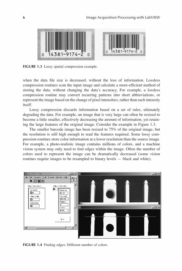
Lossy compression discards information based on a set of rules, ultimatelydegrading the data. For example, an image that is very large can often be resized tobecome a little smaller, effectively decreasing the amount of information, yet retain-ing the large features of the original image. Consider the example in Figure 1.3.
The smaller barcode image has been resized to 75% of the original image, butthe resolution is still high enough to read the features required. Some lossy com-pression routines store color information at a lower resolution than the source image.For example, a photo-realistic image contains millions of colors, and a machinevision system may only need to Þnd edges within the image. Often the number ofcolors used to represent the image can be dramatically decreased (some visionroutines require images to be resampled to binary levels � black and white).
FIGURE 1.3
Lossy spatial compression example.
FIGURE 1.4
Finding edges: Different number of colors.
1480_book.fm Page 6 Tuesday, June 24, 2003 11:35 AM

Image Types and File Management
7
Consider the example in Figure 1.4. An edge detection routine has beenexecuted on two similar images. The Þrst is an 8-bit grayscale image (whichcontains 256 colors), and the second is a binary (2 colors) image. Although theamount of color data has been signiÞcantly reduced in the second image, the edgedetection routine has completed successfully. In this example, decreasing theimage�s color depth to a binary level may actually improve the detection of edges;the change between background and object is from one extreme to the other,whereas the steps in the 256-color image are more gradual, making the detectionof edges more difÞcult.
1.2.1.1 JPEG
Of the Þve image Þle formats that the Vision Toolkit supports by default, JPEG(Joint Photographic Experts Group) Þles are probably the most common. The JPEGformat is optimized for photographs and similar continuous tone images that containa large number of colors, and can achieve astonishing compression ratios, even whilemaintaining a high image quality. The JPEG compression technique analyzes images,removes data that is difÞcult for the human eye to distinguish, and stores the resultingdata as a 24-bit color image. The level of compression used in the JPEG conversionis deÞnable, and photographs that have been saved with a JPEG compression levelof up to 15 are often difÞcult to distinguish from their source images, even at highmagniÞcation.
1.2.1.2 TIFF
Tagged Image File Format (TIFF) Þles are very ßexible, as the routine used tocompress the image Þle is stored within the Þle itself. Although this suggests thatTIFF Þles can undergo lossy compression, most applications that use the format useonly lossless algorithms. Compressing TIFF images with the Lempel-Zev-Welch(LZW) algorithm (created by Unisys), which requires special licensing, has recentlybecome popular.
1.2.1.3 GIF
GIF (CompuServe Graphics Interchange File) images use a similar LZW compres-sion algorithm to that used within TIFF images, except the bytes are reversed andthe string table is upside-down. All GIF Þles have a color palette, and some can beinterlaced so that raster lines can appear as every four lines, then every eight lines,then every other line. This makes the use of GIFs in a Web page very attractivewhen slow download speeds may impede the viewing of an image. Compressionusing the GIF format creates a color table of 256 colors; therefore, if the image hasfewer than 256 colors, GIF can render the image exactly. If the image contains morethan 256 colors, the GIF algorithm approximates the colors in the image with thelimited palette of 256 colors available. Conversely, if a source image contains lessthan 256 colors, its color table is expanded to cover the full 256 graduations, possibly
1480_book.fm Page 7 Tuesday, June 24, 2003 11:35 AM

8
Image Acquisition Processing with LabVIEW
resulting in a larger Þle size. The GIF compression process also uses repeating pixelcolors to further compress the image. Consider the following row of a raster image:
Instead of represented each pixel�s intensity discreetly, a formula is generated thattakes up much less space.
1.2.1.4 PNG
The Portable Network Graphics Þle format is also a lossless storage format thatanalyzes patterns within the image to compress the Þle. PNG is an excellent replace-ment for GIF images, and unlike GIF, is patent-free. PNG images can be indexedcolor, true color or grayscale, with color depths from 1 to 16 bits, and can supportprogressive display, so they are particularly suited to Web pages. Most image formatscontain a header, a small section at the start of the Þle where information regardingthe image, the application that created it, and other nonimage data is stored. Theheader that exists in a PNG Þle is programmatically editable using code developedby a National Instruments� Applications Engineer. You are able to store multiplestrings (with a maximum length of 64 characters) at an unlimited number of indices.Using this technique, it is possible to �hide� any type of information in a PNGimage, including text, movies and other images (this is the method used to storeregion of interest (ROI) information in a PNG Þle). The source code used to realizethis technique is available at the National Instruments Developer Zone athttp://www.zone.ni.com (enter �Read and Write Custom Strings in a PNG� in theSearch box).
1.2.1.5 BMP
Bitmaps come in two varieties, OS/2 and Windows, although the latter is by far themost popular. BMP Þles are uncompressed, support both 8-bit grayscale and color,and can store calibration information about the physical size of the image alongwith the intensity data.
1.2.1.6 AIPD
AIPD is a National Instruments uncompressed format used internally by LabVIEWto store images of Floating Point, Complex and HSL, along with calibration infor-mation and other speciÞcs.
1.2.1.7 Other Types
Although the formats listed in this chapter are the default types that the VisionToolkit can read, several third-party libraries exist that extend the range of Þle typessupported. One such library, called �The Image Toolbox,� developed by George Zou,allows your vision code to open icon (.
ico
), Windows MetaÞle (.
wmf
), ZSoft Cor-
125 125 125 125 125 125 126 126 126 126
Þ
6(125)4(126)
1480_book.fm Page 8 Tuesday, June 24, 2003 11:35 AM

Image Types and File Management
9
poration Picture (
.pcx
) Þles and more. The Image Toolbox also contains otherfunctions such as high-quality image resizing, color-grayscale and RGB-HSL con-version utilities. More information (including shareware downloads) about GeorgeZou�s work can be found at
http://gtoolbox.yeah.net
.
AllianceVision
has released a LabVIEW utility that allows the extraction ofimages from an AVI movie Þle. The utility can be used as a stand-alone appli-cation, or can be tightly integrated into the National Instruments Vision Builder(Figure 1.5).
The utility also allows the creation of
AVIs
from a series of images, includingmovie compression codecs. More information about the Alliance Vision
AVI ExternalModule for IMAQ Vision Builder
can be found at http://www.alliancevision.com.
1.3 WORKING WITH IMAGE FILES
Almost all machine vision applications work with image Þles. Whether the imagesare acquired, saved and postprocessed, or if images are acquired, processed andsaved for quality assurance purposes, most systems require the saving and loadingof images to and from a Þxed storage device.
1.3.1 S
TANDARD
I
MAGE
F
ILES
The simplest method of reading an image Þle from disk is to use
IMAQ ReadFile
.
ThisVision Toolkit VI can open and read standard image Þle types (
BMP
,
TIFF
,
JPEG
,
PNG
and
AIPD
), as well as more-obscure formats (Figure 1.6). Using
IMAQ ReadFile
with the standard image types is straightforward, as shown in Figure 1.7. Once youhave created the image data space using
IMAQ Create
, the image Þle is opened and
FIGURE 1.5
AVI external module for IMAQ vision builder.
1480_book.fm Page 9 Tuesday, June 24, 2003 11:35 AM

10
Image Acquisition Processing with LabVIEW
read using
IMAQ ReadFile
.
The image data is parsed and, if required, converted intothe type speciÞed in
IMAQ Create.
This image is then loaded into memory, andreferenced by its Image Out output. Both Image In and Image Out clusters usedthroughout the Vision Toolkit are clusters of a string and numeric; they do not containthe actual image data, but are references (or pointers) to the data in memory.
FIGURE 1.6 IMAQ ReadFile
FIGURE 1.7 Loading a Standard Image File
1480_book.fm Page 10 Tuesday, June 24, 2003 11:35 AM

Image Types and File Management 11
LabVIEW often creates more than one copy of data that is passed into sub-VIs,sequences, loops and the like, so the technique of passing a pointer instead of thecomplete image dataset dramatically decreases the processing and memory requiredwhen completing even the simplest of Vision tasks.
Saving standard image Þles is also straightforward using IMAQ WriteFile, asshown in Figure 1.8. IMAQ WriteFile has the following inputs:
Input DescriptionFile type Specify the standard format to use when writing the image to Þle. The
supported values are: AIPD, BMP, JPEG, PNG, TIFFa
Color palette Applies colors to a grayscale source image. The color palette is an array of clusters that can be constructed either programmatically, or determined using IMAQ GetPalette, and is composed of three-color planes (red, green and blue), each consisting of 256 elements. A speciÞc color is achieved by applying a value between 0 and 255 for each of the planes (for example, light gray has high and identical values in each of the planes). If the selected image type requires a color palette and if one has not been supplied, a grayscale color palette is generated and written to the image Þle.
a IMAQ WriteFile has a cluster on its front panel where TIFF Þle-saving parameters can be set (including photometric and byte order options), although this input is not wired to the connector pane. If you use the TIFF format, you should wire the cluster to the connector pane, allowing programmatic access to these options.
FIGURE 1.8 Saving a Standard Image File
1480_book.fm Page 11 Tuesday, June 24, 2003 11:35 AM

12 Image Acquisition Processing with LabVIEW
1.3.2 CUSTOM AND OTHER IMAGE FORMATS
Working with images Þles that are not included in the Þve standard types supportedby IMAQ ReadFile can be achieved either by using a third-party toolkit, or decodingthe Þle using IMAQ ReadFile�s advanced features. Consider the example in Figure1.9, which shows an image being saved in a custom Þle format. The size of theimage (x,y) is Þrst determined and saved as a Þle header, and then the image datais converted to an unsigned 8-bit array and saved as well. Opening the resulting Þlein an ASCII text editor shows the nature of the data (Figure 1.10)
The Þrst four characters in the Þle specify the x size of the image, followed bya delimiting space (this is not required, but has been included to demonstrate thetechnique), then the four characters that represent the y size of the image. Whenreading this custom Þle format, the header is Þrst read and decoded, and then theremaining Þle data is read using IMAQ ReadFile (Figure 1.11).
FIGURE 1.9 Save an image in a custom format � wiring diagram.
FIGURE 1.10 A custom Þle format image.
1480_book.fm Page 12 Tuesday, June 24, 2003 11:35 AM

Image Types and File Management 13
When setting the Þle options cluster and reading custom Þles, it is vitallyimportant to know the raw Þle�s structure. In the previous example, the values inFigure 1.12 were used.
FIGURE 1.11 Load image from a custom format � wiring diagram.
Input DescriptionRead raw Þle If set as zero, the remaining cluster options are ignored, and the routine attempts
to automatically determine the type of standard image Þle (AIPD, BMP, JPEG, PNG and TIFF); otherwise the Þle is considered a custom format
File data type Indicates how each pixel of the image is encoded; the following values are permitted:
� 1 bit� 2 bits� 4 bits� 8 bits� 16 bits (unsigned)� 16 bits (signed)� 16 bits (RGB)� 24 bits (RGB)� 32 bits (unsigned)� 32 bits (signed)� 32 bits (RGB)� 32 bits (HSL)� 32 bits (ßoat)� 48 bits (complex 2 ¥ 24-bit integers)
Offset to data The number of bytes to ignore at the start of the Þle before the image data begins; use this input when a header exists in the custom format Þle
Use min max This input allows the user to set a minimum and maximum pixel intensity range when reading the image; the following settings are permitted:
� Do not use min max (min and max are set automatically based on the extremes permitted for the Þle data type)
� Use Þle values (minimum and maximum values are determined by Þrst scanning the Þle, and using the min and max values found; the range between the min and max values are then linearly interpolated to create a color table)
� Use optional values (use the values set in the optional min value and optional max value controls)
Byte order Sets whether the byte weight is to be swapped (big or little endian; this setting is valid only for images with a Þle data type of 8 or more bits)
1480_book.fm Page 13 Tuesday, June 24, 2003 11:35 AM

14 Image Acquisition Processing with LabVIEW
FIGURE 1.12 IMAQ ReadFile - File Options
1480_book.fm Page 14 Tuesday, June 24, 2003 11:35 AM

15
2
Setting Up
You should never underestimate the importance of your image acquisition hardware.Choosing the right combination can save hours of development time and stronglyinßuence the performance of your built application. The number of cameras, acqui-sition cards and drivers is truly mind-boggling, and can be daunting for the Þrst-time Vision developer. This book does not try to cover the full range of hardwareavailable, but instead describes common product families most appropriate to theLabVIEW Vision developer.
2.1 CAMERAS
Your selection of camera is heavily dependent on your application. If you select anappropriate camera, lens and lighting setup, your efforts can then be focused (punintended!) on developing your solution, rather than wrestling with poor image data;also, appropriate hardware selection can radically change the image processing thatyou may require, often saving processing time at execution.
An electronic camera contains a sensor that maps an array of incident photons(an optical image) into an electronic signal. Television broadcast cameras wereoriginally based on expensive and often bulky Vidicon image tubes, but in 1970Boyle invented the solid state charged-coupled device (CCD). A CCD is a light-sensitive, integrated circuit that stores irradiated image data in such a way that eachacquired pixel is converted into an electrical charge. CCDs are now commonly foundin digital still and video cameras, telescopes, scanners and barcode readers. A camerauses an objective lens to focus the incoming light, and if we place a CCD array atthe focused point where this optical image is formed, we can capture a likeness ofthis image (Figure 2.1).
FIGURE 2.1
Camera schematic.
1480_book.fm Page 15 Tuesday, June 24, 2003 11:35 AM

16
Image Acquisition Processing with LabVIEW
2.1.1 S
CAN
T
YPES
The main types of cameras are broken into three distinct groups: (1) progressivearea scan, (2) interlaced area scan and (3) line scan.
2.1.1.1 Progressive Area Scan
If your object is moving quickly, you should consider using a progressive scancamera. These cameras operate by transferring an entire captured frame from theimage sensor, and as long as the image is acquired quickly enough, the motion willbe frozen and the image will be a true representation of the object. Progressive-scancamera designs are gaining in popularity for computer-based applications, becausethey incorporate direct digital output and eliminate many time-consuming processingsteps associated with interlacing.
2.1.1.2 Interlaced Area Scan
With the advent of television, techniques needed to be developed to minimize theamount of video data to be transmitted over the airwaves, while providing a satis-factory resulting picture. The standard interlaced technique is to transmit the picturein two pieces (or
Þelds
), called
2:1 Interlaced Scanning
(Figure 2.2). So an imageof the letter �a� broken down into its 2:1 interlace scanning components would yieldthe result shown in Figure 2.3.
One artifact of interlaced scanning is that each of the Þelds are acquired at aslightly different time, but the human brain is able to easily combine the interlacedÞeld images into a continuous motion sequence. Machine vision systems, on theother hand, can become easily confused by the two images, especially if there isexcessive motion between them, as they will be sufÞciently different from eachother. If we consider the example in Figure 2.3, when the object has moved to theright between the acquisition of Field A and Field B, a resulting interlaced imagewould not be a true representation of the object (Figure 2.4).
FIGURE 2.2
Interlaced scanning schematic.
Field ALine 1
Field ALine 2
Field ALine 3
Field ALine 4
Field BLine x+3
Field BLine x+2
Field BLine x+1
Field ALine xField B
Line 2x
1480_book.fm Page 16 Tuesday, June 24, 2003 11:35 AM

Setting Up
17
2.1.1.3 Interlacing Standards
2.1.1.3.1 NTSC vs. PAL
The Þrst widely implemented color television broadcast system was launched in theU.S. in 1953. This standard was penned by the National Television System Com-mittee, and hence called
NTSC
. The NTSC standard calls for interlaced images tobe broadcast with 525 lines per frame, and at a frequency of 29.97 frames per second.In the late 1950s, a new standard was born, called
PAL
(Phase Alternating Line),which was adopted by most European countries (except France) and other nations,including Australia. The PAL standard allow for better picture quality than NTSC,with an increased resolution of 625 lines per frame and frame rates of 25 framesper second.
Both of the NTSC and PAL standards also deÞne their recorded tape playingspeeds, which is slower in PAL (1.42 m/min) than in NTSC (2.00 m/min), resultingin a given length of video tape containing a longer time sequence for PAL. Forexample, a T-60 tape will indeed provide you with 60 min of recording time whenusing the NTSC standard, but you will get an extra 24 min if using it in PAL mode.
2.1.1.3.2 RS-170
RS-170 standard cameras are available in many ßavors, including both monochromeand color varieties. The monochrome version transmits both image and timinginformation along one wire, one line at a time, and is encoded using analog variation.The timing information consists of horizontal synch signals at the end of every line,and vertical synch pulses at the end of each Þeld.
The RS-170 standard speciÞes an image with 512 lines, of which the Þrst 485are displayable (any information outside of this limit is determined to be a �blanking�period), at a frequency of 30 interlaced frames per second. The horizontal resolutionis dependent on the output of the camera � as it is an analog signal, the exact
FIGURE 2.3
(a) Interlaced (b) Field A (c) Field B.
FIGURE 2.4
Interlaced image with object in motion.
1480_book.fm Page 17 Tuesday, June 24, 2003 11:35 AM

18
Image Acquisition Processing with LabVIEW
number of elements is not critical, although typical horizontal resolutions are in theorder of 400 to 700 elements per line. There are three main versions of the colorRS-170 standard, which use one (composite video), two (S-Video) or four (RGBS;Red, Green, Blue, Synchronization) wires. Similar to the monochrome standard, thecomposite video format contains intensity, color and timing information on the sameline. S-Video has one coaxial pair of wires: one carries combined intensity andtiming signals consistent with RS-170 monochrome, and the other carries a separatecolor signal, with a color resolution much higher than that of the composite format.S-Video is usually carried on a single bundled cable with 4-pin connectors on eitherend. The RGBS format splits the color signal into three components, each carryinghigh-resolution information, while the timing information is provided on a separatewire � the synch channel.
2.1.1.4 Line Scan
Virtually all scanners and some cameras use image sensors with the CCD pixelsarranged in one row. Line scan cameras work just as their name suggests: a lineararray of sensors scans the image (perhaps focused by a lens system) and builds theresulting digital image one row at a time (Figure 2.5).
The resolution of a line scan system can be different for each of the two axes.The resolution of the axis along the linear array is determined by how many pixelsensors there are per spatial unit, but the resolution perpendicular to the array (i.e.,the axis of motion) is dependent on how quickly it is physically scanning (or
stepping
). If the array is scanned slowly, more lines can be acquired per unit length,thus providing the capability to acquire a higher resolution image in theperpendicular axis. When building an image, line scan cameras are generally usedonly for still objects.
FIGURE 2.5
Line scan progression.
1480_book.fm Page 18 Tuesday, June 24, 2003 11:35 AM

Setting Up
19
A special member of the Line Scan family does not scan at all � the linedetector. This type is often used when detecting intensity variations along one axis,for example, in a spectrometer (Figure 2.6).
As the light diffracts through the prism, the phenomenon measured is the relativeangular dispersion, thus a two-dimensional mapping is not required (although severalsuch detectors actually use an array a few pixels high, and the adjacent values areaveraged to determine the output for their perpendicular position of the array).
2.1.1.5 Camera Link
A relatively new digital standard, Camera Link was developed by a standardscommittee of which National Instruments, Cognex and PULNiX are members.Camera Link was developed as a scientiÞc and industrial camera standard wherebyusers could purchase cameras and frame grabbers from different vendors and usethem together with standard cabling. Camera Link beneÞts include smaller cablesizes (28 bits of data are transmitted across Þve wire pairs, decreasing connectorsizes, therefore theoretically decreasing camera-housing sizes) and much higher datatransmission rates (theoretically up to 2.38 Gbps).
The Camera Link interface is based on Low Voltage Differential Signaling(LVDS), a high-speed, low-power, general purpose interface standard(ANSI/TIA/EIA-644). The actual communication uses differential signaling (whichis less susceptible to noise � the standard allows for up to
±
1V in common modenoise to be present), with a nominal signal swing of 350 mV. This low signal swingdecreases digital rise and fall times, thus increasing the theoretical throughput. LVDSuses current-mode drivers, which limit power consumption. There are currently threeconÞgurations of Camera Link interface � Base, Medium and Full � each withincreasing port widths.
The Camera Link wiring standard contains several data lines, not only dedicatedto image information, but also to camera control and serial communication (camerapower is not supplied through the Camera Link cable).
More information regarding the Camera Link standard can be found in the�SpeciÞcations of the Camera Link Interface Standard for Digital Cameras andFrame Grabbers� document on the accompanying CD-ROM.
FIGURE 2.6
Spectrometer schematic.
AB
C
D
A B C D
Linear Aray
LightSource
Prism/Grating
1480_book.fm Page 19 Tuesday, June 24, 2003 11:35 AM

20
Image Acquisition Processing with LabVIEW
2.1.1.6 Thermal
Used primarily in defense, search and rescue and scientiÞc applications, thermalcameras allow us to �see� heat. Thermal cameras detect temperature changes dueto the absorption of incident heat radiation. Secondary effects that can be used tomeasure these temperature ßuctuations include:
Thermal cameras can be connected to National Instruments image acquisitionhardware with the same conÞguration as visible spectrum cameras. More informationregarding thermal cameras can be found at the
FLIR Systems
Web site(http://www.ßir.com).
IndigoSystems
also provides a large range of off-the-shelf and custom thermalcameras that ship with native LabVIEW drivers. More information on their productscan be found at http://www.indigosystems.com.
2.1.2 C
AMERA
A
DVISORS
: W
EB
-B
ASED
R
ESOURCES
Cameras come in all shapes, sizes and types; choosing one right for yourapplication can often be overwhelming. National Instruments provides an excellentonline service called �Camera Advisor� at http://www.ni.com (Figure 2.7).
Using this Web page, you can search and compare National Instruments testedand approved cameras by manufacturer, model, vendor, and speciÞcations. There isalso a link to a list of National Instruments tested and approved cameras from the�Camera Advisor� page. Although the performance of these cameras is almostguaranteed to function with your NI-IMAQ hardware, you certainly do not have touse one from the list. As long as the speciÞcations and performance of your selectedcamera is compatible with your hardware, all should be well.
Another excellent resource for cameras and lenses system is the Graftek Web site(http://www.graftek.com; Figure 2.8). Graftek supplies cameras with NI-IMAQ driv-ers, so using their hardware with the LabVIEW Vision Toolkit is very simple. TheGraftek Web site also allows comparisons between compatible products to be madeeasily, suggesting alternative hardware options to suit almost every vision system need
Type Description
Thermoelectric Two dissimilar metallic materials joined at two junctions generate a voltage between them that is proportional to the temperature difference. One junction is kept at a reference temperature, while the other is placed in the path of the incident radiation.
Thermoconductive A
bolometer
is an instrument that measures radiant energy by correlating the radiation-induced change in electrical resistance of a blackened metal foil with the amount of radiation absorbed. Such bolometers have been commercially embedded into arrays, creating thermal image detectors that do not require internal cooling.
Pyroelectric Pyroelectric materials are permanently electrically polarized, and changes in incident heat radiation levels alter the surface charges of these materials. Such detectors lose their pyroelectric behavior if subject to temperatures above a certain level (the Curie temperature).
1480_book.fm Page 20 Tuesday, June 24, 2003 11:35 AM

Setting Up
21
FIGURE 2.7
National Instruments Camera Advisor.
FIGURE 2.8
The Graftek website.
1480_book.fm Page 21 Tuesday, June 24, 2003 11:35 AM

22
Image Acquisition Processing with LabVIEW
2.1.3 U
SER
S
OLUTION
: X-R
AY
I
NSPECTION
S
YSTEM
Neal Pederson holds an M.S. in Electrical Engineering from Northwestern PolytechnicUniversity, and is the president of VI Control Systems Ltd., based in Los Alamos,NM. His company, an NI Alliance Program Member, offers years of experience insoftware and hardware development of controls for complex systems such as linearaccelerators and pulse-power systems, data acquisition in difÞcult environments andsophisticated data analysis. Neal can be contacted by e-mail at [email protected].
2.1.3.1 Introduction
The 1-MeV x-ray inspection system will inspect pallets and air cargo containers inorder to identify contraband (including drugs and weapons) without the need formanual inspection. While speciÞcally designed to inspect air cargo pallets and aircargo containers, it can be used to inspect virtually any object that can Þt throughthe inspection tunnel (Figure 2.9) such as machinery, cars and vans, and materialsof all types.
The system combines two new technologies: the Nested High Voltage Generator(NHVG), a proprietary technology of North Star Research Corp., and MeVScan(U.S. Patent #6009146), a magnetically controlled moving x-ray source with astationary collimator. It produces x-ray pencil beams for transmission and scatterimaging. Two transmission images are produced, 30û apart. This gives the operatora stereoscopic, three-dimensional view of the inspected cargo and increases thelikelihood of seeing objects hidden behind other objects. Additionally, a backscatterimage is produced. These 3 images are processed and displayed separately at theoperator�s control console.
FIGURE 2.9
X-Ray inspection system.
1480_book.fm Page 22 Tuesday, June 24, 2003 11:35 AM

Setting Up
23
2.1.3.2 Control and Imaging Hardware Configuration
The remote computer control system is mounted in a bay of four 24-in. wide racks.There are four 21-in. monitors controlled by one computer and a multi-monitorvideo card. There is also one CRT with four video sources that is used for videosurveillance of the system. One of the four computer monitors is used for controllingthe scan process and for entering user and pallet information. The other threemonitors are used to display and manipulate the three x-ray images (Transmission1, Transmission 2 and Backscatter). The images are generated by acquiring PMTdata on a PCI-6052E DAQ board. One thousand vertical pixels are acquired for eachx-ray scan. This is duplicated 1000 times in the horizontal direction while palletsare moving on the conveyors to create a 1000
¥
1000 pixel image for each of thethree images. A PC-TIO-10 timing board carefully times the x-ray system and thedata collection. The Remote Device Access Server (RDA) that is built into NI-DAQand a Þber-optic Ethernet link allow the data to be acquired from a remote computer.This isolates the operator�s console from high voltage and prevents EMI/RFI prob-lems. RDA provides the full 333 kS/s bandwidth of the PCI-6052E DAQ board ina double-buffered mode. All DC analog and digital controls use Group3�s Þber-optically distributed control hardware. The Group3 hardware is speciÞcally designedfor accelerator and high voltage applications where isolation is critical.
2.1.3.3 Control Software
The control software (Figure 2.10) was designed to allow operators with little or nocomputer experience to inspect pallets without having any knowledge of how thex-ray machine works. This meant that a very complicated process of control, con-ditioning and fault detection had to be totally automated. This was accomplished by
FIGURE 2.10
Control screen.
1480_book.fm Page 23 Tuesday, June 24, 2003 11:35 AM

24
Image Acquisition Processing with LabVIEW
using a series of LabVIEW state machines. Four state machines were used to handlethe major control processes:
1.
Cold start procedure:
initial log-on and vacuum system conditioning2.
Warm start procedure:
repeat log-ons and NHVG preparation3.
Scan procedure
: conveyor automation, x-ray generation and image datacollection
4.
Fault/reset procedure
: fault handling and system reset
The automatic state machines control approximately 200 I/O points. A mainte-nance mode will bypass the automatic state machines and allow maintenance per-sonnel to control any I/O point individually. This was very useful during systemdevelopment and troubleshooting.
A system administrator screen allows the system administrator to provide names,passwords and access levels to users. User names are included in the header of eacharchived image and passwords prevent regular users from going into the maintenanceand administrator modes.
2.1.3.4 Imaging Software
The imaging software handles display and manipulation of x-ray image data. Theimaging functions run on separate screens and take advantage of the multi-threadedparallel loop capabilities that are built into LabVIEW. There are three screensdedicated to image manipulation; each screen has an x-ray image, a thumbnail copyof the x-ray image and a control palette for controlling image functions (Figure 2.11).
When image data is acquired, the data is Þrst processed and then buffered in 16 bitinteger format. A fourth x-ray detector is used to normalize the data while it is beingcollected. Because the x-ray detectors pick up cosmic rays from outer space, asoftware routine is used to eliminate them before display. By double-buffering thedata while it is being collected, the Transmission 1 image is updated 20 scans at atime while the images are being acquired. Transmission 2 and Backscatter imagesare updated after the scan is complete. The 16 bit data is converted to Unsigned 8bit integer format before it is displayed on the screen as 256 grayscale.
Data for the x-rays has much higher resolution than can be seen with 256grayscale. A process called
window and level
is used to �see into� the x-ray data.The window and level routine allows the operator to set the upper and lower depthsof x-ray penetration that is displayed for each image. This has the affect of beingable to see through materials of different densities.
IMAQ Vision is used to display and manipulate the image data. These functionsinclude zoom, pan, reverse video, edge enhance and 3-D position, which is used toÞnd the vertical height of an object after the operator makes a selection on each ofthe two stereoscopic transmission images. A thumbnail of each image displays theentire image in a 250
¥
250 pixel area. If the image is zoomed beyond 1
¥
, theoperator can simply click on the portion of interest in the thumbnail image and thezoomed image will pan to this portion of the image.
1480_book.fm Page 24 Tuesday, June 24, 2003 11:35 AM

Setting Up
25
2.1.3.5 Conclusions
The combination of LabVIEW, IMAQ Vision and NI-DAQ RDA provided a completeand economical virtual instrumentation solution to the control of a very complex x-ray machine. Other software and hardware packages could have done each piece ofthis system, but it would have been difÞcult and expensive to integrate. LabVIEWprovided fast software development that could leverage off other Windows technol-ogies such as multi-monitor video cards and TCP/IP communications. IMAQ Visionprovided powerful imaging tools that easily combined the data acquisition andcontrol capabilities of LabVIEW. NI-DAQ RDA provided a seamless integrationbetween high-speed DAQ boards and a remotely isolated control location.
FIGURE 2.11
X-Ray imaging screen (front half of a van).
1480_book.fm Page 25 Tuesday, June 24, 2003 11:35 AM

26
Image Acquisition Processing with LabVIEW
2.2 IMAGE ACQUISITION HARDWARE
Image acquisition hardware is the physical interface between your PC and camera,such as frame grabbers and embedded interfaces that come standard with most PCs.
2.2.1 N
ATIONAL
I
NSTRUMENTS
F
RAME
G
RABBERS
National Instruments image acquisition hardware (Figure 2.12) is often the Þrstchoice for developers using LabVIEW and the Vision Toolkit. It works seamlesslywith the software, and is speciÞcally designed for integration with other NationalInstruments products such as DAQ, motion control and CAN hardware.
National Instruments has a small range of image acquisition cards for both PCI andPXI (Figure 2.13) architectures, and they all have either the RTSI or PXI trigger buses,which makes synchronizing IMAQ and DAQ very simple and accurate. Although itsIMAQ hardware is often considered expensive, the quality and functionality of the cardsoften outweighs the excessive cost of subsequent development time when a card froma different vendor is chosen. Comprehensive information on the National Instrumentsimage acquisition hardware range can be found at http://www.ni.com.
2.2.2 IEEE 1394 (F
IRE
W
IRE
) S
YSTEMS
First conceived in the distant past (as far as PC technology is concerned), the IEEE1394 standard enables simple, high-bandwidth data interfacing between computers,peripherals and consumer electronics products.
FIGURE 2.12
A populated PXI-1020.
(a) (b)
FIGURE 2.13
(a) National Instruments Frame Grabber (NI-1409). (b) IMAQ cards in a PXI rack.
1480_book.fm Page 26 Tuesday, June 24, 2003 11:35 AM

Setting Up
27
Apple Computer technologists (www.apple.com) deÞned the standard in 1986,naming it
FireWire
in reference to the high data speeds that it could sustain � farquicker than any other technology of its type at the time. Adopted by the IEEE in1995, FireWire has become extremely popular as PC and operating system vendorsinclude embedded support for it. For example, both Dell Computers (www.dell.com)and Microsoft
®
Windows
®
(www.microsoft.com/windows) now include native sup-port for FireWire hardware, and National Instruments retails a Measurement andAutomation Explorer plug-in that extends its capability to interfacing with FireWirecameras.
The high data rates of FireWire, the ability to mix real-time and asynchronousdata on a single connection, and simultaneous low-speed and high-speed devices onthe same network are all very strong reasons to use FireWire hardware. The FireWirebus can have up to 63 devices simultaneously connected, although IEEE 1394.1 busbridges will soon be available, extending the capability to more than 60,000 devices.There are currently three standard IEEE 1394 signaling rates: S100 (98.304 Mbps),S200 (196.608 Mbps) and S400 (393.216 Mbps), although two new standards thatshould be available very soon will reach speeds of approximately 800 and 1200Mbps. Thankfully, these faster busses are designed to support existing lower speeddevices as well, and even mixed speeds simultaneously.
Getting data into your PC requires an IEEE 1394 adapter, which can either bea PCI card, or an integrated interface (Figure 2.14). There are two accepted plug-socket standards: six-pin (shown on the PCI card in Figure 2.14(a)) and four-pin(Figure 2.14(b)). The IEEE 1394 standard deÞnes that the six-pin systems containtwo separately shielded twisted pairs for data transmission, plus two power conduc-tors and an overall external shield. These power conductors are used to supply powerto devices on the bus (between 8 and 30 volts DC, with a maximum loading of 1.5A), whereas the smaller four-pin conductors are for data transmission only. This isparticularly important to remember when attempting to connect devices that drawtheir power from the IEEE 1394 bus, as they will not work when using the four-pinvariety.
FireWire cables are limited to 4.5 m between devices, although restricting thespeed of the bus to the S200 standard allows a distance increase to approximately
(
a) (b)
FIGURE 2.14
(a) PCI IEEE 1394 card. (b) Integrated laptop IEEE 1394 port.
1480_book.fm Page 27 Tuesday, June 24, 2003 11:35 AM

28
Image Acquisition Processing with LabVIEW
14 m. The use of IEEE 1394 repeaters (Figure 2.15) has become common when thefull S800 speed is required, and IEEE 1394 transceivers have been announced thatare powered by in-wall wiring and extend the distance between active nodes to atleast 70 m using plastic optical Þber.
As noted previously, these quoted distances are between each device, so a standardnetwork containing many FireWire devices can be up to 63 devices
¥
4.5 m = 283.5 m.There are a large number of FireWire cameras currently available (Figure 2.16),
including models from Basler Vision Technologies (www.baslerweb.com), Sony(www.sony.com), unibrain (www.unibrain.com) and SVS-VISTEK GmbH(www.svs-vistek.com).
More information regarding the IEEE 1394 standard and applicable hardwarecan be found at the IEEE 1394 Trade Association Web site (http://www.1394ta.org).
FIGURE 2.15
IEEE 1394 repeater.
FIGURE 2.16
IEEE 1394 camera with lens.
1480_book.fm Page 28 Tuesday, June 24, 2003 11:35 AM

Setting Up
29
2.2.3 USB S
YSTEMS
Although very inexpensive,
universal serial bus
(USB) cameras often sufÞce whenyour image acquisition needs are simple (Figure 2.17). USB cameras are small,easily connected to your PC, and do not require a frame grabber card.
There are currently two USB standards: the original version is able to handledata rates of 1.5 Mbps, whereas the new version (USB 2.0) can transmit at 12 Mbps.USB 2.0 can theoretically reach transfer rates of 480 Mbps; however, there is a widevariation in edge rates. With typical line loads, full speed devices usually fall in the12 to 25 ns range, and low-speed devices typically range 110 to 225 ns.
The USB standard allows for a limit of 127 devices to be connected simulta-neously, although devices often reserve large ranges of the available bandwidth, sothis limit is rarely practically achievable. If a large number of devices are required,you can install extra USB interfaces in your PC, effectively providing independentUSB buses and raising the number of devices that will function simultaneously. USBcable lengths are limited to 5 m due to a cable delay speciÞcation of 26 ns thatallows for signal reßections to settle in the cable before any subsequent bits aretransmitted.
Both USB and IEEE 1394 are serial buses; IEEE 1394 can move more data ina given amount of time, but is considerably more expensive than USB. Applicationsthat are best suited for FireWire are high-bandwidth applications (e.g., external diskdrives and high-quality video streams), whereas USB Þlls the middle- and low-bandwidth application niche (including Webcams, audio, scanners and printers).
National Instruments does not provide native support for USB cameras, althoughseveral LabVIEW drivers are available. One such solution is Peter Parente�s
WebcamLibrary,
which is featured in Chapter 3.More information regarding the USB standards and applicable hardware can be
found at the USB Implementers Forum Web site (http://www.usb.org).
FIGURE 2.17
An inexpensive webcam with a USB interface.
1480_book.fm Page 29 Tuesday, June 24, 2003 11:35 AM

30
Image Acquisition Processing with LabVIEW
2.3 FROM OBJECT TO CAMERA
Often the physical constraints of the object you are monitoring or existing hardwarearound it will control the placement of your camera, lens system and lighting. Beforeyou buy any hardware, you should consider several factors.
2.3.1 R
ESOLUTION
The resolution of a camera system refers to the smallest feature of the object thatit can distinguish. A common example used to demonstrate resolution is a barcode,shown in Figure 2.18. As you can see, a barcode is made from black and white bars
of varying width. If the resolution of your acquisition system is too coarse toresolve between the smallest black and white bars, then useful data will be lost,and you will not be able to resolve the barcode. One common solution is to usethe highest resolution system available, and then you will never lose useful data.However, there are several reasons not to choose this option: it requires moreprocessing power and memory, is much slower and is much more expensive. Thetricky part is to determine a suitable compromise, and therefore most efÞcient andeconomical resolution.
As a general rule, your smallest useful object feature should be at least 2 pixels.If so, you can be assured of never missing it due to its image falling on an inactivepart (sections between each of the CCD array elements) of your detector. Althoughthat sounds simple, you need to consider the lens system that you are using to focusyour image on the detector array. For example, using a 2
¥
zoom system willeffectively increase the resolution of your image, but decrease its Þeld of vision. Todetermine the sensor resolution, you will require to achieve a smallest feature of 2pixels, you can use the following equation:
The sensor resolution is a dimensionless quantity; use the same units for boththe Þeld of view and smallest feature to achieve a useful answer. For example, whenreading a barcode 35 mm long, with a narrow bar of 0.75 mm, through a lens systemof 1
¥
magniÞcation, the sensor resolution would need to be at least:
FIGURE 2.18
Barcode.
Sensor Resolution1 2D
FieldOfViewSmallestFeature
= ÊË
�¯
ÈÍÍ
ùúú
Sensor Resolution1 235
0 7594D pixels= Ê
Ë�¯
ÈÍÍ
ùúú
=.
1480_book.fm Page 30 Tuesday, June 24, 2003 11:35 AM

Setting Up
31
Although this would be useful for a barcode (as the information you are attempt-ing to acquire is basically a one-dimensional line proÞle across the code), mostdetector arrays are two-dimensional, so this equation needs to be applied across bothdimensions. Another example is measuring the size of an apple. Consider a particularvariety of apple, which has a maximum horizontal size of 8 cm, its vertical size willnot exceed 10 cm, and the required accuracy of the measurement needs to be 1 mm(0.001 m). The minimum sensor resolution is determined as:
indicating a sensor with a resolution of at least 160
¥
200 is required.
2.3.2 D
EPTH
OF FIELD (DOF)
The DOF of a lens system is the lens-perpendicular spatial range of which objectsremain in focus; any objects outside of the DOF will not be in focus. The DOF isdirectly related to the blur diameter, as shown in Figure 2.19. Consider a beam (agroup of adjacent rays) of light traveling from the object through the lens andfocusing on the CCD array of a camera. As the beam travels through the lens, itundergoes geometric aberration, both spatially and temporally, so the beam defo-cuses. If the beam is defocused enough to cover an area of the CCD that is largerthan the required resolution (the blur spot), then the image will be out of focus. Thisphenomenon also can occur due to chromatic aberration, which is evident whendifferent frequencies of light (e.g., colors in the visible spectrum) are diffracted atdifferent angles.
One method of increasing DOF is to place a limiting iris in front of the lens(Figure 2.20).Unfortunately, using this method causes less light to irradiate the lens,so you will need to increase the amount of light falling on the object to achievesimilar contrast levels.
FIGURE 2.19 Depth of Þeld.
Sensor ResolutionH
mm
pixels= ÊË
�¯
ÈÍÍ
ùúú
=20 080 001
160..
Sensor ResolutionV
mm
pixels= ÊË
�¯
ÈÍÍ
ùúú
=20 100 001
200..
Lens
Object
BlurDiameter
Depth Of Field
1480_book.fm Page 31 Tuesday, June 24, 2003 11:35 AM

32 Image Acquisition Processing with LabVIEW
2.3.3 CONTRAST (OR MODULATION)
Contrast is often referred to as �resolution�s brother.� Resolution is the ability toresolve spatial differences in your image, while contrast is the ability to resolveintensity differences. Contrast is therefore a dimensionless quantity that is the dif-ference between the lightest and darkest features of an image:
As this equation suggests, when the difference between IBrightest and IDarkest ishigh, the contrast tends toward 1 (unity), indicating that the image has a large rangeof contrast. Conversely, when the image is �ßat� and has very little contrast, thecontrast value approaches 0. In an example image
FIGURE 2.20 Decreased iris.
123 122 117 125 134
132 120 115 122 133
131 121 118 125 132
133 125 119 127 130
132 129 120 122 129
Lens
Object
BlurDiameter
Original DOF
IrisIris Extended DOF
ContrastI I
I Iwhere I I IBrightest Darkest
Brightest DarkestBrightest Darkest Darkest=
-+
> π , 0
I IBrightest Darkest= =134 115,
1480_book.fm Page 32 Tuesday, June 24, 2003 11:35 AM

Setting Up 33
indicates a low-contrast image, whereas the following example image:
indicates an image with a high-contrast level. A high-contrast image often appearsto be sharper than that of a lower contrast image, even when the acquired image isof identical resolution.
2.3.4 PERSPECTIVE (PARALLAX)
Perspective errors occur when the object�s surface is not perpendicular to the cameraaxis (Figure 2.21). The second image is quite badly distorted (skewed) due to thehigh angle between the object�s surface and the camera axis.
Perspective errors occur in just about every lens system that exists, unless theonly object feature that you are interested in is directly below the camera axis, andis only a few pixels wide. There are two common methods of minimizing perspectiveerror: software calibration and telecentricity.
123 180 193 221 247
186 183 149 173 185
255 208 89 143 136
250 210 11 78 102
246 205 15 101 66
\ = -+
=Contrast134 115134 115
0 076.
I IBrightest Darkest= =255 11,
\ = -+
=Contrast255 11255 11
0 917.
1480_book.fm Page 33 Tuesday, June 24, 2003 11:35 AM

34 Image Acquisition Processing with LabVIEW
2.3.4.1 Software Calibration
Calibration occurs when an object with known features is acquired, and thedifferences between the known object and the acquired image are used to processsubsequently acquired images. The Vision Toolkit ships with several intuitivecalibration routines and known grids to help make calibration easier. Consider thestandard Vision Toolkit Calibration Grid in Fi gure 2.22. This grid is provided
with the Vision Toolkit as a PDF document, and can found using the followingpath: Start > Programs > National Instruments > Vision > Documentation >Calibration Grid.
The calibration grid�s dots have radii of 2 mm and center-to-center distances of1 cm, although this may vary slightly depending on your printer setup (using a high-
FIGURE 2.21 Camera perspectives.
FIGURE 2.22 Calibration grid.
Minimal Perspective Error High Perspective Error
Image Image
1480_book.fm Page 34 Tuesday, June 24, 2003 11:35 AM

Setting Up 35
resolution printer will improve the accuracy of a calibration). National Instrumentssuggests that once you have printed it out:
� The displacement in the x and y directions be equal.� The dots cover the entire desired working area.� The radius of the dots is 6 to 10 pixels.� The center-to-center distance between dots range from 18 to 32 pixels.� The minimum distance between the edges of the dots is 6 pixels.
If you cannot print the grid to the speciÞcations recommended by NationalInstruments, you can purchase preprinted grids from several companies such asEdmund Industrial Optics (go to http://www.edmundoptics.com and type �calibra-tion target� in the Search box). If we acquire an image of a calibration grid usingthe same camera setup as described previously, the perspective error is quite apparent(Figure 2.23).
2.3.4.2 Telecentricity
Telecentricity occurs in dedicated multi-element lens systems when all of the chiefrays for all points across the object are collimated (parallel to the optical axis) (Figure2.24). Telecentricity can be difÞcult to visualize, as it provides nearly constantmagniÞcation over a range of working distances, virtually eliminating perspectiveangle error across the face of the lens.
Consider a car approaching you. As it gets closer, it looks larger, but if it isviewed with a telecentric lens, its size will not change while it is in the lens�telecentric range. Another advantage of using a telecentric lens is the parallel nature
FIGURE 2.23 Calibration grid with perspective error.
FIGURE 2.24 Telecentricity.
LensSystem
CCDArray
1480_book.fm Page 35 Tuesday, June 24, 2003 11:35 AM
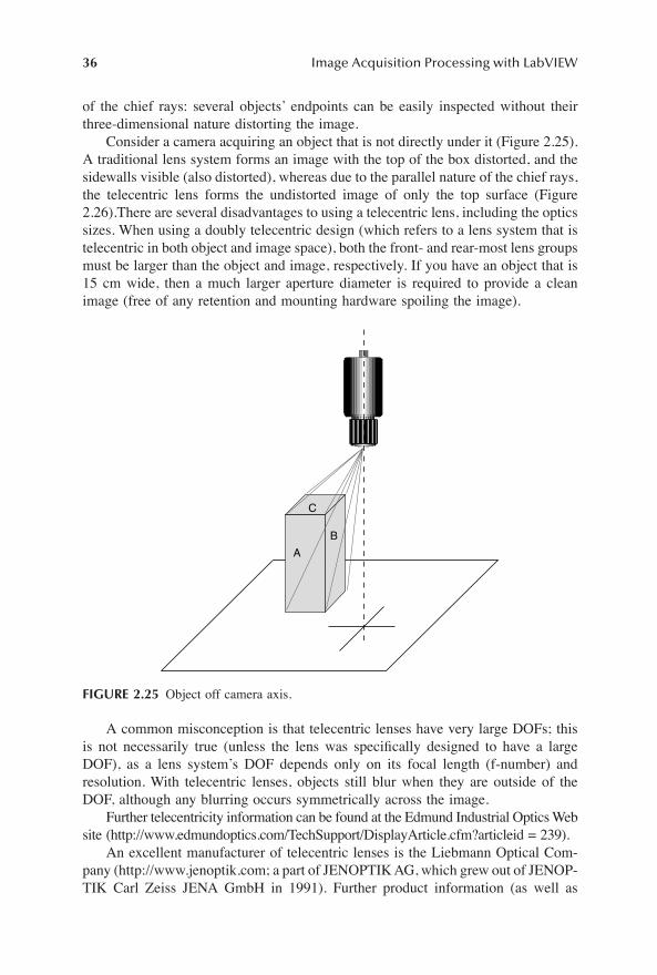
36 Image Acquisition Processing with LabVIEW
of the chief rays: several objects� endpoints can be easily inspected without theirthree-dimensional nature distorting the image.
Consider a camera acquiring an object that is not directly under it (Figure 2.25).A traditional lens system forms an image with the top of the box distorted, and thesidewalls visible (also distorted), whereas due to the parallel nature of the chief rays,the telecentric lens forms the undistorted image of only the top surface (Figure2.26).There are several disadvantages to using a telecentric lens, including the opticssizes. When using a doubly telecentric design (which refers to a lens system that istelecentric in both object and image space), both the front- and rear-most lens groupsmust be larger than the object and image, respectively. If you have an object that is15 cm wide, then a much larger aperture diameter is required to provide a cleanimage (free of any retention and mounting hardware spoiling the image).
A common misconception is that telecentric lenses have very large DOFs; thisis not necessarily true (unless the lens was speciÞcally designed to have a largeDOF), as a lens system�s DOF depends only on its focal length (f-number) andresolution. With telecentric lenses, objects still blur when they are outside of theDOF, although any blurring occurs symmetrically across the image.
Further telecentricity information can be found at the Edmund Industrial Optics Website (http://www.edmundoptics.com/TechSupport/DisplayArticle.cfm?articleid = 239).
An excellent manufacturer of telecentric lenses is the Liebmann Optical Com-pany (http://www.jenoptik.com; a part of JENOPTIK AG, which grew out of JENOP-TIK Carl Zeiss JENA GmbH in 1991). Further product information (as well as
FIGURE 2.25 Object off camera axis.
A
B
C
1480_book.fm Page 36 Tuesday, June 24, 2003 11:35 AM

Setting Up 37
several other brands of lenses and machine vision components) can be found at theAdept Electronic Solutions Web site: (http://www.adept.net.au).
2.3.5 NATIONAL INSTRUMENTS LENS PARTNERS
National Instruments has several lens partners that have been selected due to theirwide range of quality lens systems designed to assist you in completing a visionsystem. These partners include Edmund Industrial Optics (http://www.edmundop-tics.com), Navitar (http:/ /www.navitar.com), InÞnity Photo-Optical(http://www.inÞnity-usa.com) and Graftek Imaging (http://www.graftek.com).Graftek Imaging�s Web site has a �lens selector.� You can specify lens parameters,and it will not only Þnd all possible matches within their product range, but alsodisplay possible compatible products for comparison (Figure 2.27).
2.4 LIGHTING
Lighting is an important, yet often overlooked facet of image acquisition � lightingcan make or break your system. Some system integrators have been known toconsider the industrial lighting solution a low-priority task, to be quickly decided
FIGURE 2.26 Traditional vs. telecentric lens systems.
FIGURE 2.27 The Graftek lens selector Website.
A
CB
C
Traditional Telecentric
1480_book.fm Page 37 Tuesday, June 24, 2003 11:35 AM

38 Image Acquisition Processing with LabVIEW
upon toward the very end of the project during the implementation phase. Althoughthis approach can be fruitful, selecting an appropriate lighting apparatus during theproject deÞnition stage can drastically change the path of your development process.Selecting a different illumination solution, rather than investing in higher resolutiondetectors and imaging lenses, can improve often image quality. Although machinevision lighting hardware can come in many shapes and sizes, the most commontypes are area array, backlight, dark Þeld and ring and dome illuminators. Specializedtypes include cloudy day, diffuse on axis, collimated on axis and square continuousdiffuse illuminators.
2.4.1 AREA ARRAYS
Area array illuminators are by far the most common machine vision lighting devices,and are typically used on nonspecular surface objects with low reßection. Thephysical makeup of an area array is a matrix of small lights (often LEDs) coveringa large area, thus creating a wide beam of light toward the object. The most commonarea array variants include spot and ßat area array sources (as shown in Figure 2.28).Area array sources are often the cheapest solution to general purpose light applica-tions, and are especially useful when the light source is required to be some distancefrom the object (spot lighting).
2.4.2 RING
Ring illumination is a popular choice for applications that require coaxial lighting,and can produce uniform illumination when used at appropriate distances. As thering can be placed around the viewing axis, the object is irradiated almost as thoughthe light is projecting from or behind the camera itself (Figure 2.29). When used inthis method, the resulting image generally has few shadows. Ring lighting is onlyuseful when illuminating nonreßective surfaces, otherwise circular glare patterns arereßected (Figure 2.30).
FIGURE 2.28 (a) Area array schematic. (b) Area array.
Camera
Light Source
Object
(a) (b)
1480_book.fm Page 38 Tuesday, June 24, 2003 11:35 AM

Setting Up 39
Ring lighting is often used in areas such as microscopy, photographic documen-tation, medical and biological research, metallurgical and forensic inspection, semi-conductor etching and printing inspection. Ring lights are particularly useful whenilluminating objects at short working distances, otherwise its effects become similarto a point source or area array.
2.4.3 DARK FIELD
The light emitted from dark Þeld illuminators (Figure 2.31) provides low-angleillumination, enhancing the contrast of surface features, and displaying the contoursof the object, including engraved marks and surface defects.
FIGURE 2.29 (a) Ring schematic. (b) Ring
FIGURE 2.30 Reßective object illuminated with a ring light.
Camera
Object
Light Source
(a) (b)
1480_book.fm Page 39 Tuesday, June 24, 2003 11:35 AM

40 Image Acquisition Processing with LabVIEW
Dark Þeld lights cast shadows from the object, much like an edge detectionimage processing routine will enhance the perceived edges (where there is a largevariation in intensity) in an image. The physical layout of the illuminator is similarto ring lighting, except that the illuminator is placed closer to the object, and thelight is angled inward (Figure 2.32).
2.4.4 DOME
Dome illuminators provide diffused uniform light, evenly illuminating three-dimen-sional surfaces, and therefore produce very few shadows. The dome light source isrelatively close to the object under inspection. Domes lack 100% on-axis capability,leaving the light/camera aperture visible in the center of resulting images. If thatarea is not part of the region of interest, domes can offer a cost-effective alternativeto continuous diffuse illuminators (Figure 2.33).
FIGURE 2.31 (a) Dark Field schematic; (b) Dark Þeld.
(a) (b)
FIGURE 2.32 (a) Semireßective object illuminated with a ring light. (b) The same objectilluminated with a dark Þeld light.
Camera
Object
(a) (b)
Light Source
1480_book.fm Page 40 Tuesday, June 24, 2003 11:35 AM

Setting Up 41
2.4.5 BACKLIGHTS
Backlights are useful in providing silhouettes and enhanced images of internalcomponents of clear or semiclear objects (Figure 2.34).
In Figure 2.35, a lamp globe Þlament is difÞcult to resolve using a ring lightfor illumination, as excess light pollution is reßected from the glass surface. Thisreßected light is eradicated when the globe is backlit with a diffuse source, allowingmuch easier Þlament recognition. Backlights can also be useful in detecting cavitiesin semitransparent objects, and surface-to-surface breaches in opaque objects (e.g.,drilled holes). Image processing can then be useful to count, map and classify theseartifacts.
FIGURE 2.33 (a) Dome schematic. (b) Dome Þeld.
FIGURE 2.34 (a) Backlight schematic. (b) Backlight.
Camera
ObjectLight Source(off axis)
(a) (b)
Camera
Backlight
Object
(a) (b)
1480_book.fm Page 41 Tuesday, June 24, 2003 11:35 AM

42 Image Acquisition Processing with LabVIEW
2.4.6 CONTINUOUS DIFFUSE ILLUMINATOR (CDI™)
CDI creates almost inÞnitely diffuse light, and is particularly useful when inspectinghighly specular surfaces where any reßections may cause a vision system to seedefects generated by reßected light pollution (Figure 2.36).
CDIs emulate cloudy days where only nonparallel diffuse light rays emanatefrom the sky. CDI applications include packaged component inspection, e.g., phar-maceutical blister-packages and electronic component tubes. The printed foil exam-ple in Figure 2.37 shows the reßected light when the object is illuminated with aring light; it makes pattern recognition and therefore character recognition verydifÞcult, whereas the diffuse multi-angled light decreases the glare from light pol-lution dramatically when using a CDI.
FIGURE 2.35 (a) Reßective object illuminated with a ring light. (b) The same object illu-minated with a backlight.
FIGURE 2.36 (a) Cloudy day schematic. (b) Cloudy day illuminator.
Camera
Object
BeamSplitter
LightSource(off-axis)
LightSource(on-axis)
(a) (b)
1480_book.fm Page 42 Tuesday, June 24, 2003 11:35 AM

Setting Up 43
2.4.7 DIFFUSE ON AXIS LIGHTS (DOAL™) AND COLLIMATED ON AXIS LIGHTS (COAL)
DOAL and COAL lights use beam splitter technology to illuminate the object asthough the camera is on the same axis as the light source (Figure 2.38).
If desired, the light source can seem to be virtually at the same point as the camera.Specular surfaces perpendicular to the camera appear illuminated, while surfaces atan angle to the camera appear darker. Nonspecular surfaces absorb the incident lightand appear dark. DOAL illuminators emit diffuse light, whereas COAL illuminatorsare designed for applications requiring coaxial bright light. The electronic circuit boardexample in Figure2.39 shows that the contrast achieved from the DOAL setup is muchhigher than if a ring light was used. This makes pattern recognition and calipermeasurement much more reliable in an automated vision application.
FIGURE 2.37 (a) An object illuminated with a ring light. (b) The same object illuminatedwith a CDI.
FIGURE 2.38 (a) DOAL schematic. (b) DOAL illuminator.
Camera
Object
Diffuser
LightSource
BeamSplitter
1480_book.fm Page 43 Tuesday, June 24, 2003 11:35 AM

44 Image Acquisition Processing with LabVIEW
Unfortunately, DOALs often have a low reßected light throughput to the camera,such that you may need to invest in multiple sources to provide sufÞcient detectorirradiation.
2.4.8 SQUARE CONTINUOUS DIFFUSE ILLUMINATORS (SCDI™)
SCDI illuminators take the DOAL (described earlier) design to another level, pro-viding signiÞcantly greater uniformity of diffuse illumination (Figure 2.40).
SCDIs are particularly suited to moderately faceted and undulating specularsurfaces. Common examples of SCDI applications include compact disk artworkveriÞcation and the inspection of solder patterns on circuit boards ( Figure 2.41).
FIGURE 2.39 (a) PCB tracks illuminated with a ring light. (b) Illuminated with a DOAL.
FIGURE 2.40 (a) SCDI schematic. (b) SCDI illuminator.
Camera
Object
Diffuser
LightSource
BeamSplitter
(a) (b)
1480_book.fm Page 44 Tuesday, June 24, 2003 11:35 AM

Setting Up 45
FIGURE 2.41 (a) PCB pads illuminated using a ring light. (b) Illuminated with a SCDI.
1480_book.fm Page 45 Tuesday, June 24, 2003 11:35 AM

L1626_C01.fm Page 1 Wednesday, June 18, 2003 4:07 PM

47
3
Image Acquisition
There are two main methods of obtaining images: loading from disk and acquiringdirectly using a camera. Image acquisition is often considered a complex task, butit can be simpliÞed for most vision applications. National Instrument�s Measurementand Automation Explorer (MAX), LabVIEW and the Vision Toolkit make imageacquisition a straightforward and integrated task.
3.1 CONFIGURING YOUR CAMERA
The range of cameras available to use with your vision system is astounding � severaldifferent types exist across brand lines (more information of camera types can befound in Chapter 2). If you are using a National Instruments image acquisition card,MAX depends on a camera deÞnition Þle to understand the conÞguration of thecamera attached to the card. ConÞguration Þles for common cameras are includedwith a standard NI-IMAQ installation (Figure 3.1)
An icd Þle contains all of the information MAX and subsequently IMAQ needs toacquire images and control the camera. Figure 3.2 illustrates an example icd Þle. Asshown, the icd Þle is of a human-understandable format, and can be manually editedusing
Notepad
, or a similar ASCII text editor. As the camera conÞguration Þle extensionis
icd
, the Windows
®
operating system should not have an application registered tolaunch the Þle type by default; therefore, you will need to manually open the Þle for
FIGURE 3.1
icd Þle directory.
1480_book.fm Page 47 Tuesday, June 24, 2003 11:35 AM

48
Image Acquisition Processing with LabVIEW
viewing and editing. These Þles reside in the \National Instruments\NI-IMAQ\Data\directory on your hard disk.
Be sure to select the icd Þle that matches both your camera and frame grabber.The icd Þle�s name often describes the appropriate interface to use with the Þle; forexample, camera Þles will often have an interface sufÞx denoting the interface type:
Camera_Name.icdCamera_Name(1409).icdCamera_Name(BNC).icd
If your camera does not have a corresponding icd Þle listed in the directoryabove, camera vendors will often provide one for you, or it may be available fromNational Instruments. The National Instruments FTP site stores icd Þles for commoncameras, and can be accessed at ftp://ftp.ni.com/support/imaq/camera_support(Figure 3.3).
Fortunately, if you cannot obtain an appropriate Þle from the camera vendor,you can either create one, or copy and modify a Þle with a similar conÞguration toyour camera.
If you are using a IEEE 1394 (FireWire) camera, an icd Þle is not required.NI-IMAQ will create one when the camera is detected. The created Þles areplaced in the \National Instruments\NI-IMAQ for IEEE 1394\Data directory.Once you have a camera interface installed, you can set its properties usingMAX (Figure 3.4).
Under
Devices
and
Interfaces
, right click on the interface (or camera namein the case of a FireWire camera), and select properties (Figure 3.5).
FIGURE 3.2
A example icd Þle.
1480_book.fm Page 48 Tuesday, June 24, 2003 11:35 AM

Image Acquisition
49
Depending on the hardware installed and the capabilities of your camera, youcan set conÞguration parameters such as
brightness, autoexposure, sharpness, whitebalance, saturation, gamma, shutter speed, gain
and
iris
.
FIGURE 3.3
National Instruments icd Þle FTP site.
FIGURE 3.4
MAX camera conÞguration.
1480_book.fm Page 49 Tuesday, June 24, 2003 11:35 AM

50
Image Acquisition Processing with LabVIEW
3.2 ACQUISITION TYPES
There are four image acquisition types supported in the Vision Toolkit: Snap, Grab,Sequence and StillColor. Although the type your application needs may at Þrst seemobvious, taking the time to understand the different types could save unnecessarydevelopment time and computation during postacquisition processing.
NI-IMAQ image acquisition often uses information regarding the open IMAQsession. To determine a plethora of camera, image and session properties, you can
FIGURE 3.5
MAX camera properties.
FIGURE 3.6
IMAQ session properties.
1480_book.fm Page 50 Tuesday, June 24, 2003 11:35 AM

Image Acquisition
51
use a property node
1
(Figure 3.6). The property node example in Figure 3.8 returnsthe
image type
of the session, which is determined by either camera initialization,or is set dynamically. This
image type
value can then be passed to
IMAQ Create,
reserving the correct number of bytes per pixel for the acquired image data.
3.2.1 S
NAP
Acquiring an image using
IMAQ Snap
is the simplest type of image acquisition(Figure 3.7). Used for slow acquisition rates,
IMAQ Snap
requires just three stepsto execute: initialize, acquire and close. To initialize the IMAQ session, the
interfacename
(or the
camera name
in the case of an FireWire interface) is input to
IMAQ Init
,which opens the camera by loading and parsing its
icd
Þle from disk (as determinedby the Measurement and Automation Explorer), and opening an IMAQ session(Figure 3.8).
The IMAQ session refnum is then fed into a property node, which is set todetermine the image type of the camera interface. The dataspace for the image is
1
The FireWire image acquisition VIs do not use a property node for setting acquisition properties. Use
IMAQ1394 Attribute
to set properties, and
IMAQ1394 Attribute Inquiry
to read properties.
FIGURE 3.7
Simple snap example.
FIGURE 3.8
Simple snap example � wiring diagram.
1480_book.fm Page 51 Tuesday, June 24, 2003 11:35 AM

52
Image Acquisition Processing with LabVIEW
created, and the system then waits for the user to click either
Acquire
or
Quit
. If theuser clicks
Acquire
,
IMAQ Snap
is called (if
IMAQ Init
has not been previouslycalled, the image acquisition board is now initialized, increasing the delay beforeacquisition), and the next available video frame from the camera is returned as
ImageOut
. Finally, the IMAQ session is closed and the camera and interface resourcesreleased by calling
IMAQ Close
.
3.2.2 G
RAB
Depending on the frame rate of the camera, grabbing images from an interface bufferis a very fast method of image acquisition. Using
IMAQ Grab
is the best method ofacquiring and displaying live images (Figure 3.9). After the IMAQ session has beeninitialized,
IMAQ Grab Setup
is executed. Describing this VI as a �setup� VI is aslight misnomer, as it actually starts the camera acquiring images.
IMAQ GrabAcquire
is used to grab the current image in the camera buffer.
IMAQ Grab Acquire
has a Boolean input that deÞnes when the next image is to be acquired: synchronizedon the next vertical blank (i.e., wait for the next full image), or immediately transferthe current image (or part thereof) from the buffer.
A series of images can also be acquired using
IMAQ Snap
, but as it initializesthe image interface every time it is called, the acquisition rate can be very slow (inthe order of one frame per second) (Figure 3.10).
3.2.3 S
EQUENCE
When you know how many images you want to acquire and at what rate, a sequenceacquisition is often appropriate. You can control the number of frames and which
FIGURE 3.9
Simple grab acquisition � wiring diagram.
FIGURE 3.10
Looped Snap example.
1480_book.fm Page 52 Tuesday, June 24, 2003 11:35 AM

Image Acquisition
53
frames to acquire using
IMAQ Sequence
. In Figure 3.11, a number of images arecreated (in the for loop), and an array of those images is passed to
IMAQ Sequence
.Once
IMAQ Sequence
is called, it acquires the next number of frames as deÞnedby the number of images passed to it. The time taken to acquire the frames isdetermined by the frame rate:
For example (Figure 3.12), a unibrain� Fire-i400 1394 camera can acquire imagesat a frame rate of up to 30 frames per second. If you require 100 frames to beacquired, the acquisition would take:
IMAQ Sequence
also has a
Skip Table
array input, which allows you to deÞnea table of which frames to acquire and those to skip. The
Skip Table
array is deÞnedas each element representing the number of frames to skip before acquiring each
FIGURE 3.11
Simple sequence example � wiring diagram.
FIGURE 3.12
Simple sequence example.
AcquisitionTime sNumberOfFramesFrameRate Hz
( )( )
=
AcquisitionTimeHz
s
=
ª
10030
3 3.
1480_book.fm Page 53 Tuesday, June 24, 2003 11:35 AM

54
Image Acquisition Processing with LabVIEW
corresponding buffer. Therefore, the number of elements in the
Skip Table
shouldbe the same as the number of elements in the
Images In
array. The number of skippedframes in the Skip Table should also be considered when calculating the acquisitiontime.
3.3 NI-IMAQ FOR IEEE 1394
Image acquisition is a little different when using an IEEE 1394 (FireWire) camerainstead of a National Instruments frame grabber. To use a FireWire camera, you willeither need to access third-party camera drivers, or use the National Instrumentsgeneric driver,
NI-IMAQ for IEEE 1394
(Figure 3.13). Installing
NI-IMAQ for IEEE1394
enables access to FireWire cameras from MAX, and adds a subpalette to the
Motion and Vision
function palette (Figure 3.14).The IEEE 1394 function palette contains VIs that replace the standard NI-IMAQ
image acquisition VIs. All of the example VIs in this chapter have been replicatedwith IEEE 1394 capabilities on the accompanying CD-ROM (Figure 3.15).
FIGURE 3.13
NI-IMAQ for IEEE 1394.
FIGURE 3.14
IMAQ IEEE-1394 Function Palette.
1480_book.fm Page 54 Tuesday, June 24, 2003 11:35 AM

Image Acquisition
55
FIGURE 3.15
Simple snap example (IEEE 1394).
1480_book.fm Page 55 Tuesday, June 24, 2003 11:35 AM

56
Image Acquisition Processing with LabVIEW
3.4 USER SOLUTION: WEBCAM IMAGE ACQUISITION
Peter Parente holds his B.S. in computer engineering and computer science fromRensselaer Polytechnic Institute (RPI). His interest in inexpensive image acquisitioncame about as part of his work with the Center for Initiatives in Pre-College Edu-cation (CIPCE) at RPI (see http://www.cipce.rpi.edu for more information). Peteris currently pursuing an additional degree in computer science with a focus oncomputer graphics at the University of North Carolina�Chapel Hill.
Version 1.4 of the Webcam VIs can be found on the CD-ROM accompanyingthis book. The most recent version can be found at http://www.mindofpete.org.
3.4.1 I
NTRODUCTION
Much of the image acquisition functionality of LabVIEW has remained out of thehands of the typical consumer because of the often prohibitively high prices of pro-fessional-grade image acquisition hardware. In many cases, the image quality providedby these expensive pieces of equipment goes far beyond the needs of LabVIEWprogrammers. Many LabVIEW applications can beneÞt from merely having imagesof a process displayed on the front panel, possibly with some simple image enhance-ment applied by the Vision Toolkit. In such cases, standard acquisition devices canseem overly complex, and deÞnitely too pricey for their intended use (Figure 3.16).
Several inexpensive solutions currently exist, but generally they are drivers forparticular models and brands of cameras, and are often operating-system dependent.One attempt at adding such functionality appeared in RoboLab, a system developedby Lego, National Instruments, and Tufts University that allows users to program theLego Robotics from within the LabVIEW environment. Version 2.5 of this applicationintroduced support for the Lego Vision Command USB camera � a Logitech Quick-Cam housed in a special Lego casing. While RoboLab now allows the robotics hobbyistto capture and process image data using LabVIEW tools, it lacks support for manynew versions of Windows, and often captures at a slow rate of about two frames persecond at a resolution of 320
¥
240
¥
24. Additionally, the functionality is nested deepwithin the RoboLab software, proving less useful for those who wish to use thefunctionality directly within LabVIEW.
Another attempt has been made at Þlling the niche for LabVIEW support ofinexpensive imaging hardware, and has so far proven to be quite successful. The open
t
FIGURE 3.16
Single Capture with Display.
1480_book.fm Page 56 Tuesday, June 24, 2003 11:35 AM

Image Acquisition
57
source LabVIEW Webcam library, released in July 2002, allows images to be capturedon machines running nearly any version of Windows at speeds of 7 to 10 frames persecond at 320
×
240
×
24 resolution. The library relies on a simple dynamic link library(DLL) that communicates with the Video for Windows (VFW) programming interfacein order to initiate, configure, begin and end a capture session with an imaging device.Labeling it a “Webcam library” is a slight misnomer, as VFW allows for communicationwith practically any imaging device with a fully supported Windows driver.
3.4.2 F
UNCTIONALITY
The Webcam library consists of two sets of VIs built around the low-level function-ality of the DLL. The first set assists in the capturing of images using the DLLdescribed previously. The second set provides a means of converting captured imagesto the IMAQ format for processing, to the LabVIEW picture format for display onthe front panel, and to the bitmap format for file storage. When used together, thecapture and conversion VIs provide a straightforward means of acquiring and work-ing with image data from consumer-grade devices. A number of example uses ofthe Webcam library are provided in the subsequent discussions.
3.4.2.1 Single and Continuous Capture with Display
Only two VIs are required to capture a single image from an imaging device anddisplay it on the front panel. The Webcam
Snapshot VI
can be coupled with theWebcam
Flat to Picture VI
to accomplish this goal as shown in Figure 3.17.
A slightly more complex configuration of VIs is required to capture imagescontinuously. The Webcam
Snapshot VI
used in the single-shot acquisition shownin Figure 3.17 initializes a session, grabs a single image, and then immediately closesthe session. A similar approach is taken when performing a continuous capture,except that the grab, conversion and display operations are repeated inside a loop,with the necessary initialization and discarding VIs outside, as shown in Figure 3.18.
3.4.2.2 Single Capture with Processing and Display
Any Webcam library image can easily be converted to the IMAQ format for imageprocessing and analysis using the LabVIEW Vision Toolkit. The Webcam
Flat toIMAQ VI
is capable of creating a new buffer or using an existing IMAQ buffer to
FIGURE 3.17
Continuous Capture with Display.
1480_C03.fm Page 57 Tuesday, June 24, 2003 2:48 PM

58
Image Acquisition Processing with LabVIEW
hold image data captured from an imaging device. The resulting IMAQ image canbe used with any of the Vision Toolkit VIs. Likewise, any processed images fromthe Toolkit can be converted back into the picture format using the Webcam
IMAQto Picture VI
for display. The block diagram in Figure 3.19 demonstrates conversionsto and from the IMAQ format to perform a binary threshold operation on a singlecaptured image and display the result.
3.4.2.3 Continuous Capture with Processing and Display
Processing can also be done within a continuous capture session by including thenecessary VIs within the capture loop. The one notable difference is that the IMAQimage is created outside of the loop and passed to the Webcam
Flat to IMAQ VI
.The block diagram in Figure 3.20 demonstrates continuous image acquisition, pro-cessing and display loop.
3.4.2.4 Future Work
The Webcam library represents a solid step forward in providing robust, intuitiveand inexpensive image acquisition functionality in LabVIEW. However, the libraryitself can still be improved by the addition of error reporting, and extended to runon operating systems other than Windows. The project is under an open sourcelicense, allowing all those who wish to improve or modify the library the freedomto do so.
FIGURE 3.18
Single Capture with Processing and Display.
FIGURE 3.19
Continuous Capture with Processing and Display.
1480_C03.fm Page 58 Tuesday, June 24, 2003 2:48 PM
Image Acquisition 59
3.5 OTHER THIRD-PARTY IMAGE ACQUISITION SOFTWARE
In addition to Peter Parente�s Webcam Image Acquisition suite, Irene He has devel-oped a functional toolkit called IVision, which can acquire images from FireWireand USB cameras. IVision also contains VIs that control some of the camera settings,including focus, zoom, hue, saturation, brightness, frame rate and image size (pro-viding your hardware supports these features). The software also allows reading andwriting of several image Þle formats (BMP, DIB, JPEG, PNG, PBM, PGM, PPM,TIFF, and more), and simple image-manipulation functions. One of the IVisionToolkit�s best features is the free availability of source code, so recompilation toprevious LabVIEW versions is possible. More information about IVision (includinga downloadable version) is at http://www.geocities.com/irene_he/IVision.html.
3.6 ACQUIRING A VGA SIGNAL
An interesting tidbit of information recently cropped up on the National Instru-ments Developer Zone: how to acquire a VGA video signal from a computer�svideo card output. When testing the way your software operates, it may beadvantageous to inspect a screen shot of your application. If you attempt toacquire an image of your screen using a camera, many unwanted artifacts maybe observed: glare from the screen, mismatched refresh rates causing distortionbars and limited process repeatability. It is possible to �tap� into the 15-pin VGAD-sub connector on the back of your video card and use an NI-1409 to acquirethe video signal directly. The following video modes are supported using thistechnique:
� 640 ¥ 480 70 Hz� 640 ¥ 480 60 Hz
More information (including the VGA connector wiring diagram, icd Þles andfurther instructions) can be found by visiting http://www.zone.ni.com and entering�Using the IMAQ 1409 to Acquire a VGA Video Signal from a PC Video Card� inthe Search box.
3.7 TWAIN IMAGE ACQUISITION
TWAIN is an image capture API Þrst released in 1992, and typically used as aninterface between image processing software and a scanner or digital camera. Theword TWAIN is from Kipling�s The Ballad of East and West (�...and never the twainshall meet...�), reßecting the difÞculty, at the time, of connecting scanners to PCs(a TWAIN acronym contest was launched, with the de facto winner being TechnologyWithout An Interesting Name). Graftek and AllianceVision have released LabVIEWTWAIN drivers that allow direct access to TWAIN-compliant scanners and cameras,and import of images into LabVIEW and the Vision Toolkit. More information canbe found at http://www.alliancevision.com/net/twain/fr_twain.htm.
1480_book.fm Page 59 Tuesday, June 24, 2003 11:35 AM

60
Image Acquisition Processing with LabVIEW
3.8 USER SOLUTION: COMBINING HIGH-SPEED IMAGING AND SENSORS FOR FAST EVENT MEASUREMENT
Bryan WebbMarketing ManagerMicrosys Technologies Inc.Tel 905 678-3299 x3600Email: [email protected]
3.8.1 T
HE
C
HALLENGE
A series of customers needed systems to control automotive safety for short durationairbag and seatbelt pretensioner tests. The systems required high-speed cameras anddata acquisition, and needed to generate various control signals. Customers alsoasked for the ability to view and analyze the collected test data. The challenge wasto design and construct a highly integrated and automated product based on standardoff-the-shelf hardware that could be easily configured in the field for the differentapplications and tests.
3.8.2 T
HE
S
OLUTION
National Instruments LabVIEW software was used to control NI-DAQ, NI-DMM andField Point hardware in addition to the high-speed imagers and other ancillary equip-ment and safety interlocks. A companion program (also written in LabVIEW) providessophisticated viewing and analysis capability for both image and sensor data.
The automotive market requires the ability to design and build thousands ofparts that go together to construct a car. Consumers have embraced safety as asaleable concept, and manufacturers want to provide products that fill that need. Inaddition, the U.S. government mandates specific tests and pass-performance levelsthat must be observed. Original equipment manufacturers have outsourced somedesign work to Tier 1 and Tier 2 companies such as Autoliv, TRW, JCI, Magna/Intier,Delphi and Visteon, who supply parts and perhaps complete systems or interiors tocompanies higher up the production chain. This process has reduced in-house teststaff in many companies, often leading to the purchase of commercial test systemsrather than building complex one-off systems in-house, where learning curves canbe long, steep and therefore costly.
The stages of a product’s life include
engineering
(design validation, total per-formance testing) and
production
(product verification, lot acceptance testing, orconformity to production). Overall, testing helps validate appropriate designs, verifyappropriate production, and thus limit waste and liability. The question is, “what totest?” For example, one could simply perform an electrical or physical inspectionon a crude airbag deployment (without any triggered video or data monitoring) justto see if the bag deploys. However, there is still a question of determining whetherit deploys correctly, as per the product specification.
1480_C03.fm Page 60 Tuesday, June 24, 2003 4:22 PM
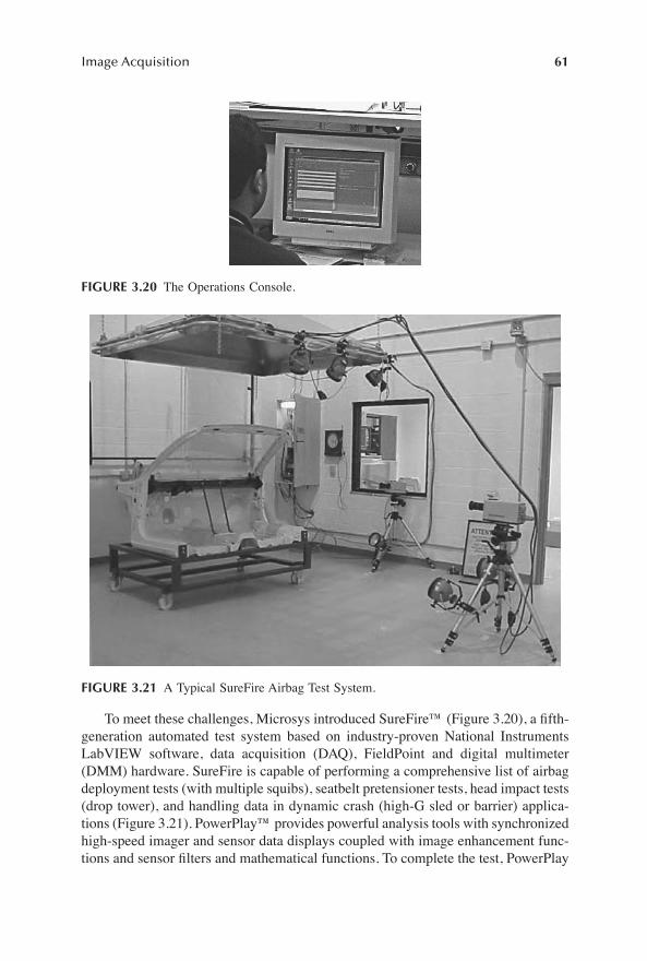
Image Acquisition 61
To meet these challenges, Microsys introduced SureFire� (Figure 3.20), a Þfth-generation automated test system based on industry-proven National InstrumentsLabVIEW software, data acquisition (DAQ), FieldPoint and digital multimeter(DMM) hardware. SureFire is capable of performing a comprehensive list of airbagdeployment tests (with multiple squibs), seatbelt pretensioner tests, head impact tests(drop tower), and handling data in dynamic crash (high-G sled or barrier) applica-tions (Figure 3.21). PowerPlay� provides powerful analysis tools with synchronizedhigh-speed imager and sensor data displays coupled with image enhancement func-tions and sensor Þlters and mathematical functions. To complete the test, PowerPlay
FIGURE 3.20 The Operations Console.
FIGURE 3.21 A Typical SureFire Airbag Test System.
1480_book.fm Page 61 Tuesday, June 24, 2003 11:35 AM

62
Image Acquisition Processing with LabVIEW
supports the creation of multiple image movies in AVI format for distribution andExcel™-based test reports.
3.8.3 S
YSTEM
C
ONSIDERATIONS
To ensure that the system can handle different test needs, a modular softwareapproach is used for hardware and other capabilities, which also minimizes theintegration time and effort for future developments. SureFire calls hardware drivermodules as they are required to perform different functions. A similar approach isused for other features that may be needed by one application and not another (e.g.,automatic AVI creation at the end of a test). New hardware modules can be developedand added to SureFire to meet changing test demands. The system can configureand control almost any high-speed imager by loading the appropriate driver. Forexample, if the customer needs to perform squib resistance measurements (Figure3.22), the appropriate driver module (and hardware) is added. The test system-typeand application-specific demands dictate the driver modules that accompany Sure-Fire. This allows us to tailor each system to the customer’s specific requirements atthe time of shipping and for later system upgrades.
Each SureFire Test System installation has its own unique combination of hard-ware — variable quantities and types of safety interlocks, climactic chamber con-trols, imager systems, and sensor channels — which all require system interfacingand control. It is important in any test scenario to produce repeatable and reliableresults that lead to customers being able to make informed business decisions. Oneof our key design objectives was to minimize the time between order and deliveryof the system, while keeping system costs in line with customer budgets by using
FIGURE 3.22
Setting the Squib Outputs.
1480_C03.fm Page 62 Tuesday, June 24, 2003 3:58 PM

Image Acquisition
63
industry-standard components. The powerful graphics programming available inLabVIEW (for DAQ, DMM, and FieldPoint components) was critical to the successof the system. These components provided the required flexibility and minimizedexpensive engineering time. Since 1992, the system has been evolving based oncustomer demands and feedback.
3.8.4 S
YSTEM
P
ERFORMANCE
The system was designed to dynamically configure its hardware and to control andmonitor all of the events in a specified test sequence, which the customer can designand modify without the assistance of Microsys engineers. For the most part, eachsystem is based on a standard platform, which is tailored to meet the specificcustomer requirements. During installation, the software is initially configured withcustomer specifics, including hardware modules, data entry field names, and sensordata and calibration information.
One of the unique features of SureFire is its integrated high-speed video imageand DAQ data control capability. The ability to configure and control various high-speed video imaging and DAQ equipment from a single computer simplifies testpreparation and execution, reducing user error and improving test efficiency. Fewertests are performed erroneously, leading to less scrap and lower testing costs.
SureFire is database driven (either Microsoft Access or Oracle), therefore alltest configurations, hardware calibration information and test-result pointers arestored for each test. This provides management with a tool for traceability.
For analysis, PowerPlay provides integrated video and DAQ displays to giveengineers the ability to easily correlate high-speed video images with sensor datain a fashion similar to National Instruments DIAdem. Users can also compare andevaluate multiple test results by displaying both video and sensor data from differenttests. PowerPlay will play back all open data windows in a time-synchronized fashionso that engineers can compare and confirm visual clues with sensor data. Imageenhancements include linear and angular measurements, color correction, sharpenand blur filters and edge detection and enhancement.
3.8.5 A
PPLICATIONS
Other applications for SureFire include aerospace and defense, testing products suchas ejection seats, landing shocks, missile launch (ground-based tests) and ordnance.SureFire is flexible enough to meet many applications where there is a need tointegrate and control high-speed imaging and sensors with test control. PowerPlaycan be used as a stand-alone analysis tool to combine computer-generated imageswith real test images to tweak a simulation model. PowerPlay can import and exportto data files such as DIAdem, CSV, ISO13499, TIFF, JPEG, BMP, AVI and GIF.
3.8.6 S
UMMARY
SureFire performs common automotive safety tests through its modular hardwareand software design. Each test system is tailored to meet customer requirements forsafety interlock control and monitoring, auxiliary equipment control, test trigger,
1480_C03.fm Page 63 Tuesday, June 24, 2003 3:58 PM

64 Image Acquisition Processing with LabVIEW
high-speed video capture, and sensor data acquisition. Integrated high-speed videoand DAQ hardware coupled with image enhancement and math functions provideusers with advanced test analysis capabilities.
1480_book.fm Page 64 Tuesday, June 24, 2003 11:35 AM

65
4
Displaying Images
Although not always necessary, displaying acquired and processed images to theuser is often desirable. If your application calls for the user to be able to reviewimage data, it is wise to consider performance and user interface designs veryseriously. Your Þrst question should be, �does my application
really
call for imagedata display?� Although we all like to �show off� our programming expertise, andthere is no better way than to show the users (read: managers) the before-and-afterdata, displaying images can have much more detrimental effects to system perfor-mance than traditional DAQ systems.
First, image data can often contain much more information than simple DAQdata � a voltage trace with respect to time may be only an array of a few thousanddoubles, whereas a similar application acquiring images over time could easily Þllup your RAM (e.g., a 1024
¥
768 32-bit image is approximately 3 Mb). Similarly,image data generally contains more �background� data than tradition methods,simply due to its two-dimensional nature.
Second, displaying any data on your front panel will take time and memory.Using a multithreaded version of LabVIEW, whenever you wire data to an indicator(numeric, string, Boolean, image, etc.) the
execution
thread is stopped, and thesystem switches to the
user interface
(UI) thread. The UI thread�s copy of theindicator�s data is then updated (this is generally called the
operate
data), and if thepanel is open, it is redrawn. Then the data is sent back down to the
execution thread
,but in order to do this, it is Þrst sent to a protected area of memory called the
transferbuffer
with a
mutual exclusion object
(MUTEX). After all of this is done, the systemsswitches back to the execution thread, and when it next reads data from terminals,it Þnds any new copies in the transfer buffer and uses these as the new values. Asyou can imagine, copying image data between these layers can be quite time andRAM consuming, especially if the dataset is large or inappropriately formatted.
You need to decide if you are willing to trade off system execution speed forimage display � if you do not really need to display an image on your front panel,I suggest that you do not (perhaps create a modal sub-VI that the user can view onlywhen it is required). On the other hand, you may not be able to get away from tellingthe user what is going on, but you will need to think carefully about the requiredupdate rate and how you are going to transfer the data.
4.1 SIMPLE DISPLAY TECHNIQUES
If you are reading this book, then you probably have already installed the NI Visiontoolkit, and perhaps even played around with some of the example VIs that comewith it. Figure 4.1 is a simple example that you might recognize (it has been slightlymodiÞed from its original functionality). As you can see from the comment text in
1480_book.fm Page 65 Tuesday, June 24, 2003 11:35 AM

66
Image Acquisition Processing with LabVIEW
the diagram, this example allows the user to select an image to load from disk, anddisplays it in its own ßoating window (Figure 4.2).
This technique is very simple to implement, and displaying multiple ßoatingwindows is only a little more complex.
The IMAQ WindDraw
VI has a
window
numberinput, allowing you to specify which ßoating window you want this operation to beperformed on. By default, this is set to zero, but you can specify up to 16 simultaneouswindows. Figure 4.3 demonstrates Þve simultaneous windows. This is achieved bylooping around both
IMAQ WindDraw
and
IMAQ WindClose
(Figure 4.4).Figure 4.1 and Figure 4.4 both use
IMAQ WindClose
and
IMAQ Dispose
to cleanup the ßoating windows and release the image data from memory. Technically, youcan leave the ßoating windows open, even after your VI has Þnished executing.However, this is bad form. Doing so may lead to poor memory management, withsections of the RAM continuing to be locked and therefore unusable after yourapplication has quit, forcing the user to manually close them. When you dispose animage that is still displayed, if you minimize or drag another window over it, thesystem will lose the information of the image, and will not be able to refresh thescreen correctly. Rather than dispose of each window separately, you can set the
FIGURE 4.1
Simple image display � wiring diagram.
FIGURE 4.2
Simple image display.
1480_book.fm Page 66 Tuesday, June 24, 2003 11:35 AM

Displaying Images
67
IMAQ WindClose
terminal
�Close All Windows?�
to true, and all windows currentlyopen (including any embedded windows, as discussed later) will close.
4.2 DISPLAYING IMAGES WITHIN YOUR FRONT PANEL
Although displaying your image in ßoating windows can be useful, a commonquestion asked by beginner Vision Toolkit programmers is, �how do I embed adynamic image in my front panel?� There are several methods of doing so, dependingon what you want to display and the speed restrictions you are willing to accept.
4.2.1 T
HE
I
NTENSITY
G
RAPH
The simplest method of displaying an image on a VI�s front panel is to convert itto an
intensity graph
(Figure 4.5). This method uses
IMAQ ImageToArray
(Figure4.6) to convert the image data to an array that the intensity graph can plot. Do notforget to either autoscale the z axis (intensity), or set its upper limit to an appropriatevalue (the default is 100, whereas you will probably need to set it to 255, as shownin Figure 4.5), otherwise your intensity data will be clipped.
FIGURE 4.3
Simple multiple image display.
FIGURE 4.4
Simple multiple image display � wiring diagram.
1480_book.fm Page 67 Tuesday, June 24, 2003 11:35 AM
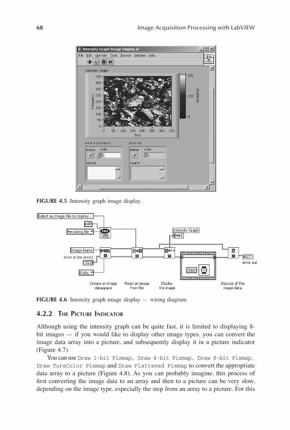
68
Image Acquisition Processing with LabVIEW
4.2.2 T
HE
P
ICTURE
I
NDICATOR
Although using the intensity graph can be quite fast, it is limited to displaying 8-bit images � if you would like to display other image types, you can convert theimage data array into a picture, and subsequently display it in a picture indicator(Figure 4.7)
You can use
Draw 1-bit Pixmap, Draw 4-bit Pixmap, Draw 8-bit Pixmap,Draw TureColor Pixmap
and
Draw Flattened Pixmap
to convert the appropriatedata array to a picture (Figure 4.8). As you can probably imagine, this process ofÞrst converting the image data to an array and then to a picture can be very slow,depending on the image type, especially the step from an array to a picture. For this
FIGURE 4.5
Intensity graph image display.
FIGURE 4.6
Intensity graph image display � wiring diagram.
1480_book.fm Page 68 Tuesday, June 24, 2003 11:35 AM

Displaying Images
69
reason, displaying images in picture controls is not generally appropriate for fre-quently updating data sets (e.g., displaying video sequences).
You need not use the IMAQ functions to load and display JPEG, PNG or BMPimages; the LabVIEW Base Development System comes with VIs to accomplishthis without installing the Vision Toolkit (Figure 4.9).
Use the appropriate VI from the
Graphics&Sound>GraphicsFormats
functionpalette (
Read JPG File, Read PNG File
or
Read BMP File
) to return the Þleas ßattened image data, and then convert it to a picture using
Draw Flattened Pixmap
(Figure 4.10). Unfortunately, if the picture indicator is not the correct size, the imagewill either be clipped or will not Þll up the entire front panel object. This problem canbe avoided by resizing the indicator to Þt the loaded image (Figure 4.12). Resizing
FIGURE 4.7
Picture control image display.
FIGURE 4.8
Picture control image display � wiring diagram.
1480_book.fm Page 69 Tuesday, June 24, 2003 11:35 AM

70
Image Acquisition Processing with LabVIEW
front panel objects can have undesired side effects. The picture indicator may becometoo large for the front panel, and even overlap other front panel objects, as shownabove (Figure 4.11).
You can also use this non-IMAQ Vision Toolkit technique to display imagesdynamically from Web addresses. A randomly chosen CRC Press Web page showsan image of a book cover, which can be displayed in a Picture indicator on a frontpanel (Figure 4.13). By using
DataSocket Read
, the raw ASCII text of the imageÞle is read, and subsequently saved to a temporary text Þle on the local hard drive.Then using the techniques described earlier, the Þle is opened, and the unßatteneddata converted to a picture (Figure 4.14).
FIGURE 4.9
Picture control image display (without IMAQ).
FIGURE 4.10
Picture control image display (without IMAQ) � wiring diagram.
1480_book.fm Page 70 Tuesday, June 24, 2003 11:35 AM
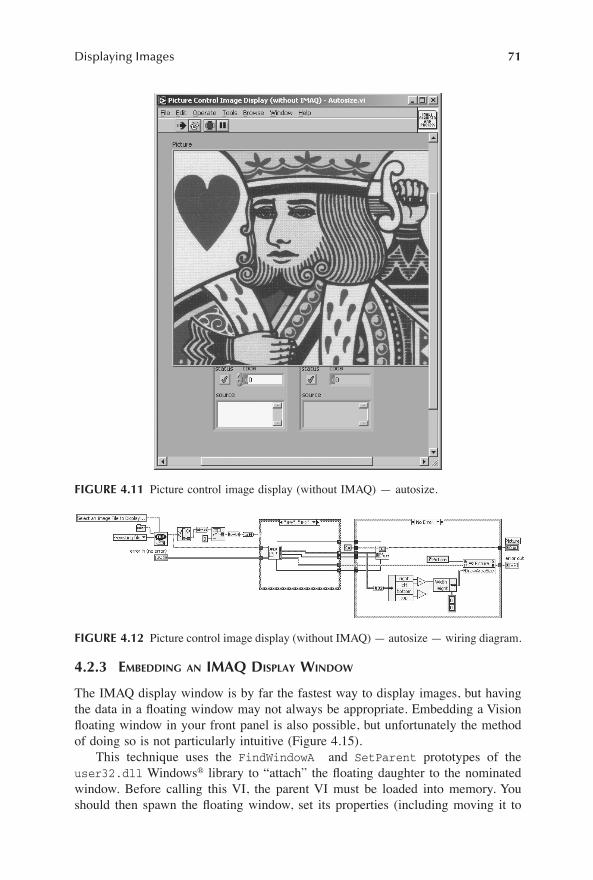
Displaying Images
71
4.2.3 E
MBEDDING
AN
IMAQ D
ISPLAY
W
INDOW
The IMAQ display window is by far the fastest way to display images, but havingthe data in a ßoating window may not always be appropriate. Embedding a Visionßoating window in your front panel is also possible, but unfortunately the methodof doing so is not particularly intuitive (Figure 4.15).
This technique uses the
FindWindowA
and
SetParent
prototypes of the
user32.dll
Windows
®
library to �attach� the ßoating daughter to the nominatedwindow. Before calling this VI, the parent VI must be loaded into memory. Youshould then spawn the ßoating window, set its properties (including moving it to
FIGURE 4.11
Picture control image display (without IMAQ) � autosize.
FIGURE 4.12
Picture control image display (without IMAQ) � autosize � wiring diagram.
1480_book.fm Page 71 Tuesday, June 24, 2003 11:35 AM
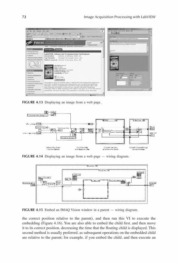
72
Image Acquisition Processing with LabVIEW
the correct position relative to the parent), and then run this VI to execute theembedding (Figure 4.16). You are also able to embed the child Þrst, and then moveit to its correct position, decreasing the time that the ßoating child is displayed. Thissecond method is usually preferred, as subsequent operations on the embedded childare relative to the parent; for example, if you embed the child, and then execute an
FIGURE 4.13
Displaying an image from a web page.
FIGURE 4.14
Displaying an image from a web page � wiring diagram.
FIGURE 4.15
Embed an IMAQ Vision window in a parent � wiring diagram.
1480_book.fm Page 72 Tuesday, June 24, 2003 11:35 AM

Displaying Images
73
IMAQ WindMove
, the coordinates that you enter are now relative to the upper leftcorner of the parent VI (including its title bar, toolbar and menu, if any).
National Instrument�s Greg McKaskle recently posted a message to the Info-LabVIEW mailing list to help clear up questions related to some confusing Windowsoperating systems terminology (for the complete transcript of the post, seehttp://messages.info-labview.org/2002/10/14/10.html):
Each window can have a parent and an owner�. Each window in LabVIEW is ownedby the LabVIEW taskbar button�s window � which is hidden by the way. Typical top-level LabVIEW panel windows do not have a parent, otherwise they would be contained(clipped and moved relative to the parent). Again, they do have an owner, but thisdoesn�t imply anything about their position, or their clipping. The owner is used tosend messages to, primarily during key processing.
Although it may look as though the child window is ßoating on top of the parentVI in the previous example, it is actually embedded; dragging, minimizing andresizing the parent affects the embedded child as though it is part of the parent�sfront panel (you can easily remove the child�s title bar by calling
IMAQ WindSetup
and setting
�Window has Title Bar?�
to false). Although the embedded child mayseem to be part of the parent, it is not. LabVIEW does not know (or care) that thechild has been embedded, and does not treat it any differently. Therefore, it is stillimportant to remember to dispose of both the embedded child window and imagedata properly (Figure 4.17).
FIGURE 4.16
Embed an IMAQ Vision window in a parent example.
1480_book.fm Page 73 Tuesday, June 24, 2003 11:35 AM

74
Image Acquisition Processing with LabVIEW
Although the child window is embedded in the parent, programming data to itis almost no different to when it was a ßoating window. However, keep in mind therelative spatial coordinates as mentioned previously, and that moving the child evenpartially outside of the parent�s bounds (Figure 4.18) will mask the image (perhapseven completely, where it may seem that your image window has disappeared). Ifyou scroll a front panel while it contains a child window, the image may not becorrectly redrawn. Therefore, it is often a good idea to disable scrolling on a frontpanel that will have an embedded IMAQ image.
4.3 THE IMAGE BROWSER
The image browser is a very useful function if you need to display a selection ofthumbnails to a user, perhaps with them selecting one (or more) for further processing.The image browser itself is displayed as a ßoating IMAQ image window (Figure 4.19).
Loading images into the image browser is quite simple. First, the browser isconÞgured, including its background color, size, style, and the number of imagesyou want displayed per line. The image browser is then displayed, like any otherimage, and populated with images. Figure 4.20 shows the image browser is updatedafter each image is inserted into it, but you could put the
IMAQ WindDraw
outsideof the for loop, causing the program to wait until all of the images have been inserted,thus displaying them all simultaneously.
FIGURE 4.17
Embed an IMAQ Vision Window in a parent example � wiring diagram.
FIGURE 4.18
Embedded window poor move example.
1480_book.fm Page 74 Tuesday, June 24, 2003 11:35 AM

Displaying Images
75
As the image browser is a ßoating IMAQ image window, you can embed it asa child into a parent VI, as discussed previously (Figure 4.21). Adding this codeembeds the image browser into the parent VI�s front panel (Figure 4.22).
One useful example of image browsers is to allow the user to select a thumb-nail, and then display (and perhaps process) the full image on the front panel ofa VI. This is achieved by embedding both the image browser and preview imageinto the parent VI, and using the selected browser thumbnail to dictate whichimage is loaded into the preview image (Figure 4.23). As not to continually loadimages into the preview image, even when the user has not selected a differentimage,
IMAQ WindLastEvent
is used to monitor if the user has clicked withinthe image browser (Figure 4.24)
FIGURE 4.19
Simple image browser example.
FIGURE 4.20
Simple image browser example � wiring diagram.
1480_book.fm Page 75 Tuesday, June 24, 2003 11:35 AM

76
Image Acquisition Processing with LabVIEW
FIGURE 4.21
Simple embedded image browser example � wiring diagram.
FIGURE 4.22
Simple embedded image browser example.
FIGURE 4.23
Image browser-selector example.
1480_book.fm Page 76 Tuesday, June 24, 2003 11:35 AM

Displaying Images
77
4.4 OVERLAY TOOLS
A picture may be worth a thousand words, but those words are often open to theviewer�s interpretation. You can give the user an enormous amount of indicativeinformation by overlaying text and other types of pictorial data over an image.
Overlaying is exactly that � placing information on top of the image. It does notreplace any of the image data (all the underlying pixels remain intact), and overlays canbe moved, changed or even removed completely with no effect on the underlying image.
4.4.1 O
VERLAYING
T
EXT
You can overlay text to describe an image to the user and provide technical,customer and company information. The fonts available to
IMAQ Overlay Text
are limited only to those installed on the local machine (the example in Figure4.25 uses
Arial
), although some of the font options (strikeout, italic, underline,outline, shadow and bold) may not be available for the font you have selected.You should remember to include any nonstandard fonts that you have used whendistributing your VIs, as they may not be installed on the target machine. If theVI cannot Þnd a user-speciÞed font, it will default to the last font successfullyselected � often with unimpressive results.
Simply supply the text, its color (you can also specify its background color butthe default is
transparent
), position coordinates and font attributes to the VI andyour text will be overlaid (Figure 4.26).
4.4.2 O
VERLAYING
S
HAPES
You can demonstrate several points or regions of interest including spatial measure-ments, using shape overlays. The default shapes include circles, rectangles and arcs(Figure 4.27). Each of the shapes have deÞnable colors, drawing bounds and Þll
FIGURE 4.24
Image browser-selector example � wiring diagram.
1480_book.fm Page 77 Tuesday, June 24, 2003 11:35 AM

78
Image Acquisition Processing with LabVIEW
options (either
Þll
or
frame), and the arc shape overlay also requires start and endangles (Figure 4.28).
4.4.3 OVERLAYING BITMAPS
Bitmap overlaying can be useful to display a company logo, a data graph image, acustom coordinate scale, or just about any other bitmap over the base image. Theexample in Figure 4.29 shows the overlaying of a company logo. The image input ofthe IMAQ Overlay Bitmap VI is unfortunately in the form of a U32 array: a standardimage input could have made life a little easier when using this function. This meansthat all images must Þrst be converted to an array before they can be overlaid. Once
FIGURE 4.25 Overlay example � text.
FIGURE 4.26 Overlay example: text � wiring diagram.
1480_book.fm Page 78 Tuesday, June 24, 2003 11:35 AM

Displaying Images 79
you have converted your image, you can also deÞne the positional coordinates of theoverlay, relative to the top left corner of the base image (Figure 4.30).
4.4.4 COMBINING OVERLAYS
As you can see, you can overlay multiple objects on a Vision window, as well asdifferent types of overlays. Figure 4.31 is an example of overlaying all of the typesdiscussed previously. Combining overlays allows a highly conÞgurable, dynamicmethod for displaying information on images, perhaps for user information, orinclusion in a printed report.
FIGURE 4.27 Overlay example � shapes.
FIGURE 4.28 Overlay example: shapes � wiring diagram.
1480_book.fm Page 79 Tuesday, June 24, 2003 11:35 AM
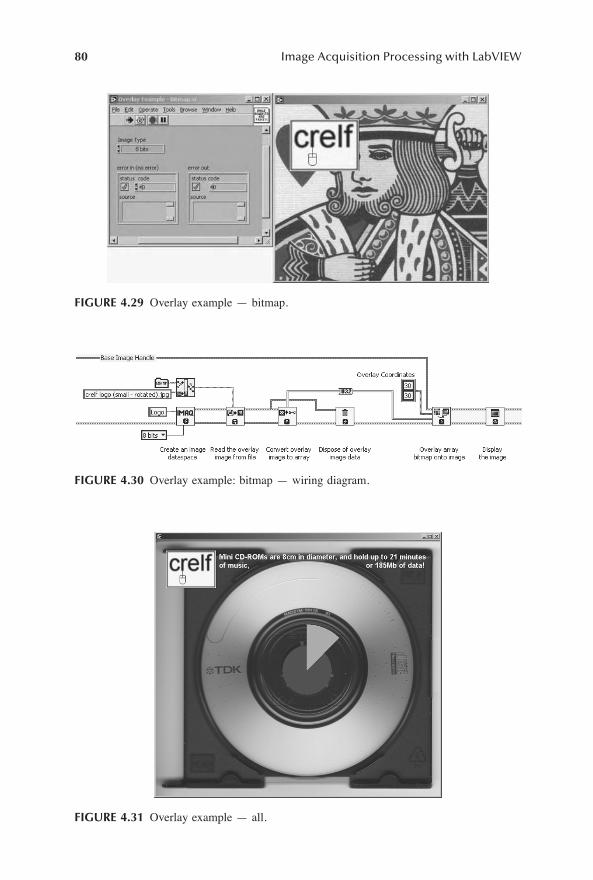
80 Image Acquisition Processing with LabVIEW
FIGURE 4.29 Overlay example � bitmap.
FIGURE 4.30 Overlay example: bitmap � wiring diagram.
FIGURE 4.31 Overlay example � all.
1480_book.fm Page 80 Tuesday, June 24, 2003 11:35 AM

Displaying Images 81
4.5 THE VISION WINDOW TOOLS PALETTE
If you need to do more than just display an image, and you are looking for some userinteraction, one often overlooked tool for the job is the Window Tools Palette (Figure4.32). This ßoating palette allows the user to select one of many tools to measure data,draw objects, zoom, pan and easily deÞne regions of interest (ROIs), while providingfeedback such as image type and current relative mouse coordinates. You display andhide the tool palette using the IMAQ WindToolsShow VI, which works in a similarmanner to IMAQ WindShow (Figure 4.33). Even before you have displayed your toolpalette, you can programmatically alter its functionality (Figure 4.34). As you see, thepalette is very customizable using IMAQ WindToolsSetup and IMAQ WindToolsMove,allowing you to deÞne which tools to display, the position of the palette, whether to showmouse coordinates, and how many tools are displayed per line (Figure 4.35).
4.5.1 AVAILABLE TOOLS
There are 13 tools available on the Vision Tools Palette (Figure 4.36):
Selection Tool (Tool 0): The selection tool allows the user to select a previ-ously deÞned ROI or shape on the image.
Point (Tool 1): The point tool allows the user to select one pixel, and can beuseful to nominate previously deÞned shapes, or return information partic-ular to that pixel (intensity or RGB values, for example).
FIGURE 4.32 Vision tools palette.
FIGURE 4.33 IMAQ WindToolsShow.
Vision Tools
Intensity Under Cursor
Image Type
Cursor Position
Object Anchor
Object Resize
1480_book.fm Page 81 Tuesday, June 24, 2003 11:35 AM

82 Image Acquisition Processing with LabVIEW
Line, Rectangle and Oval (Tools 2, 3 and 4): These tools are similar to thepoint tool, except that they offer one- (line) and two-dimensional (rectangleand oval) area selection. Figure 4.37 shows an inverse mask applied toseveral area selections, including a rectangle and oval.
FIGURE 4.34 Vision window tools palette � select tools.
FIGURE 4.35 Vision window tools palette: select tools � wiring diagram.
FIGURE 4.36 Vision window tools palette tools.
1480_book.fm Page 82 Tuesday, June 24, 2003 11:35 AM

Displaying Images 83
Polygon (Tool 5): The example above includes a demonstration of the poly-gon tool � the n-sided polygon begins with a left mouse click, and eachsubsequent side is deÞned by the next mouse click. The polygon is thenclosed to the Þrst point with a double click.
Free (Tool 6): As its name suggests, this tool allows the user to draw afreehand ßat-sided region in the image. The Þrst point is deÞned by leftclicking, as are subsequent vertices. Double clicking will close the ROI.
Annulus (Tool 7): An annulus is the area between two concentric slicedcircles. This tool is useful when analyzing parts like spanners, and terminalclamps. The two circles are initially created with a left click drag (Þrst clickdeÞnes the center of the circles, and the second deÞnes the radius of theouter circle), and then the slice and radius of the inner circle is deÞned bydragging the appropriate ROI handles.
Zoom and Pan (Tools 8 and 9): These tools allow the user to manipulatethe way an image is displayed, by either magnifying a portion of the image,to moving within the image. Zoom and pan are very useful when the userneeds to observe small areas of a large image, zooming in and then movingthe viewable area to adjacent areas.
Broken and Free-Hand Lines (Tools 10 and 11): As you can see fromFigure 4.38, broken and free lines allow the user a free way of deÞningopen and closed ROIs. The broken line creates a line as the user draws(click and drag to create the region), which is useful to trace features inthe image, whereas the free line joins the last point deÞned with the Þrst,creating a closed region.
Rotated Rectangle (Tool 12): The rotated rectangle tool is very useful whena rectangular ROI is required, but the part�s acquired image is not exactlyaligned with the coordinate system of the image acquisition system. Theuser can Þrst draw the rectangle, and then rotate it by moving one of theROI�s rotation handles.
FIGURE 4.37 Vision window tools palette � multiple tools demonstration.
1480_book.fm Page 83 Tuesday, June 24, 2003 11:35 AM
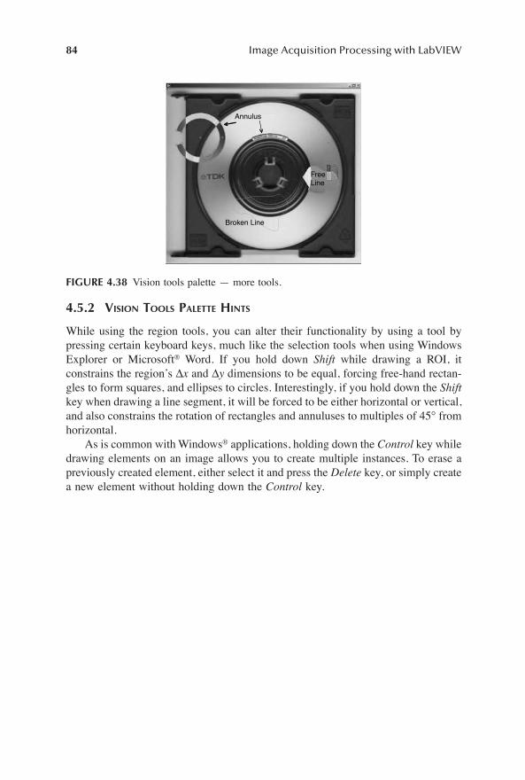
84 Image Acquisition Processing with LabVIEW
4.5.2 VISION TOOLS PALETTE HINTS
While using the region tools, you can alter their functionality by using a tool bypressing certain keyboard keys, much like the selection tools when using WindowsExplorer or Microsoft® Word. If you hold down Shift while drawing a ROI, itconstrains the region�s Dx and Dy dimensions to be equal, forcing free-hand rectan-gles to form squares, and ellipses to circles. Interestingly, if you hold down the Shiftkey when drawing a line segment, it will be forced to be either horizontal or vertical,and also constrains the rotation of rectangles and annuluses to multiples of 45∞ fromhorizontal.
As is common with Windows® applications, holding down the Control key whiledrawing elements on an image allows you to create multiple instances. To erase apreviously created element, either select it and press the Delete key, or simply createa new element without holding down the Control key.
FIGURE 4.38 Vision tools palette � more tools.
Annulus
Broken Line
FreeLine
1480_book.fm Page 84 Tuesday, June 24, 2003 11:35 AM

85
5
Image Processing
Once you have acquired images, they are often not in an appropriate format for youto analyze and must be processed Þrst. The Vision Toolkit contains many tools tohelp you clean up and alter images, from deÞning a region of interest to Þlteringand spatial manipulation.
5.1 THE ROI (REGION OF INTEREST)
A ROI is a speciÞcation structure that allows for the deÞnition of arbitrarily shapedregions within a given image, often called subimages (although a ROI can encompassthe entire image if so deÞned). A ROI contains no image data � it is not an imageitself, but a placeholder that remembers a deÞned location within an image.
Why would you need a ROI within an image? Why not just acquire the regionof interest as the complete image? There are many answers to this question: Þrst,ROIs can be irregular shapes � not necessarily the rectangle or square that yourcamera supplies. ROIs can be rectangles or squares (a square is often called an
areaof interest
, or AOI), circles, annuluses, polygons and freehand shapes. Secondly, youmay want to perform different image processing routines on different areas of animage � there is no sense in wasting valuable time on processing the whole rawimage, when you are only interested in a few small parts of it. Another reason forROIs is that you can dynamically deÞne and change them � users can draw a ROIover a portion of an image at run time, selecting their particular region of interest.
The license plate in Figure 5.1 has a deÞned ROI around the alphanumericcharacters, to make it much simpler and faster for an optical character recognition(OCR) routine to decode. Also, the routine would try to recognize characters wherenone are present, perhaps returning erroneous results.
FIGURE 5.1
Car license plate with a deÞned ROI
1480_book.fm Page 85 Tuesday, June 24, 2003 11:35 AM

86
Image Acquisition Processing with LabVIEW
By traditional deÞnition, every point of an image is either inside or outside ofa given ROI. The Vision Toolkit takes this deÞnition one step further by adding twonew ROI concepts: the line and the point. Strictly speaking, these ROI types are notactually lines and points, but a single pixel width rectangle and square respectively.Points are useful to return single value data about a region of your image (pointintensity, color data, etc) and the line can return one-dimensional information.
5.1.1 S
IMPLE
ROI U
SE
5.1.1.1 Line
A simple ROI example is that of an intensity contour measurement, as shown inFigure 5.2 and Figure 5.3. The
IMAQ
WindLastEvent
VI is used to detect the eventthat last occurred in the nominated IMAQ window and looks for a draw event(suggesting that the user has drawn a ROI of some type).
IMAQ WindGetROI
thenreturns the deÞnition of the created ROI and
IMAQ ROI Profile
returns the intensitycontours along the length of the ROI (if a two-dimensional ROI is deÞned, theintensity contours follow the outer shape of the ROI, starting at the Þrst deÞnedpoint).
As you can see, the initial ROI point is that on the far left and as the line isfollowed, the intensity levels are returned (suggesting that the background intensityof the license plate is approximately 240 units, whereas the alphanumeric charactersare approximately 50 units).
5.1.1.2 Square and Rectangle
A square ROI is the simplest two-dimensional ROI � it allows the user to select aregion with four equal sides, although the rectangle ROI is probably the most popular,allowing the user more ßexibility in deÞning the required region.
FIGURE 5.2
Simple ROI intensity contour � wiring diagram.
1480_book.fm Page 86 Tuesday, June 24, 2003 11:35 AM
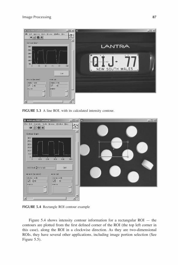
Image Processing
87
Figure 5.4 shows intensity contour information for a rectangular ROI � thecontours are plotted from the Þrst deÞned corner of the ROI (the top left corner inthis case), along the ROI in a clockwise direction. As they are two-dimensionalROIs, they have several other applications, including image portion selection (SeeFigure 5.5).
FIGURE 5.3
A line ROI, with its calculated intensity contour.
FIGURE 5.4
Rectangle ROI contour example
1480_book.fm Page 87 Tuesday, June 24, 2003 11:35 AM

88
Image Acquisition Processing with LabVIEW
Image portion selection is achieved by Þrst converting a detected ROI to arectangle and then extracting the portion of the source image that is bound by thatrectangle using
IMAQ Extract
, as shown in Figure 5.6.
5.1.1.3 Oval
An oval ROI is deÞned by Þrst holding down the left mouse button to deÞne thecenter and then dragging to deÞne the radii of the ROI:
As you can see from Figure 5.7, the position of the mouse cursor during thedrag operation may not be particularly intuitive, but it is a corner of the oval�sbounding rectangle.
5.1.2 C
OMPLEX
ROI
S
Although simple ROIs can be very useful in particular situations, several other typesare available, including the rotated rectangle and annulus arc.
FIGURE 5.5
Two-dimensional ROI image portion selection.
FIGURE 5.6
Two-Dimensional ROI image portion selection � wiring diagram.
1480_book.fm Page 88 Tuesday, June 24, 2003 11:35 AM
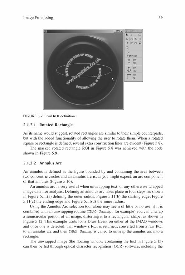
Image Processing
89
5.1.2.1 Rotated Rectangle
As its name would suggest, rotated rectangles are similar to their simple counterparts,but with the added functionality of allowing the user to rotate them. When a rotatedsquare or rectangle is deÞned, several extra construction lines are evident (Figure 5.8).
The masked rotated rectangle ROI in Figure 5.8 was achieved with the codeshown in Figure 5.9.
5.1.2.2 Annulus Arc
An annulus is deÞned as the Þgure bounded by and containing the area betweentwo concentric circles and an annulus arc is, as you might expect, an arc componentof that annulus (Figure 5.10).
An annulus arc is very useful when unwrapping text, or any otherwise wrappedimage data, for analysis. DeÞning an annulus arc takes place in four steps, as shownin Figure 5.11(a) deÞning the outer radius, Figure 5.11(b) the starting edge, Figure5.11(c) the ending edge and Figure 5.11(d) the inner radius.
Using the Annulus Arc selection tool alone may seem of little or no use, if it iscombined with an unwrapping routine (
IMAQ Unwrap,
for example) you can unwrapa semicircular portion of an image, distorting it to a rectangular shape, as shown inFigure 5.12. This example waits for a Draw Event on either of the IMAQ windowsand once one is detected, that window�s ROI is returned, converted from a raw ROIto an annulus arc and then
IMAQ Unwrap
is called to unwrap the annulus arc into arectangle.
The unwrapped image (the ßoating window containing the text in Figure 5.13)can then be fed through optical character recognition (OCR) software, including the
FIGURE 5.7
Oval ROI deÞnition.
1480_book.fm Page 89 Tuesday, June 24, 2003 11:35 AM

90
Image Acquisition Processing with LabVIEW
National Instruments OCR Toolkit add-on for the Vision Toolkit (see Chapter 8 formore information about OCR).
FIGURE 5.8
(a) Drag out a standard rectangular ROI. (b) Rotate the ROI with the handles.(c) Rotated rectangular ROI.
FIGURE 5.9
Rotated rectangle ROI image portion selection � wiring diagram.
1480_book.fm Page 90 Tuesday, June 24, 2003 11:35 AM

Image Processing
91
FIGURE 5.10
Annulus arc components.
FIGURE 5.11
(a) DeÞning the outer radius. (b) DeÞning the starting edge. (c) DeÞning theending edge. (d) DeÞning the inner radius.
Drag Point
Outer Radius
InnerRadius
Start Edge
End Edge
1480_book.fm Page 91 Tuesday, June 24, 2003 11:35 AM
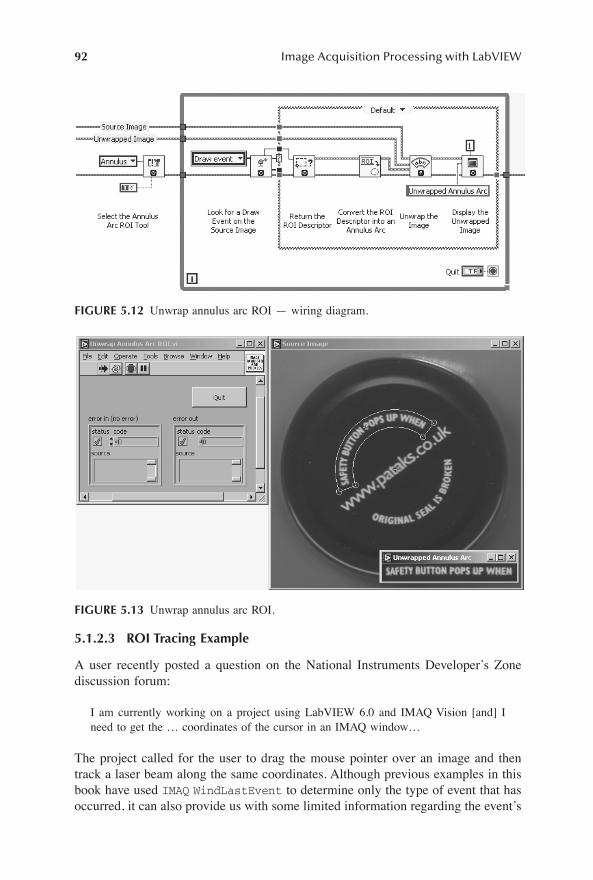
92
Image Acquisition Processing with LabVIEW
5.1.2.3 ROI Tracing Example
A user recently posted a question on the National Instruments Developer�s Zonediscussion forum:
I am currently working on a project using LabVIEW 6.0 and IMAQ Vision [and] Ineed to get the � coordinates of the cursor in an IMAQ window�
The project called for the user to drag the mouse pointer over an image and thentrack a laser beam along the same coordinates. Although previous examples in thisbook have used
IMAQ
WindLastEvent
to determine only the type of event that hasoccurred, it can also provide us with some limited information regarding the event�s
FIGURE 5.12
Unwrap annulus arc ROI � wiring diagram.
FIGURE 5.13
Unwrap annulus arc ROI.
1480_book.fm Page 92 Tuesday, June 24, 2003 11:35 AM

Image Processing
93
attributes. The VI has three outputs of interest:
event, coordinates
and
other param-eters,
which are populated as shown in Table 5.1.
In this instance, the user was able to use the
draw vertices
data returned in the
coordinates
array, which was subsequently built into an array of clusters (eachcontaining the
x,y
pair of the pixels that were traced over). This allowed the user totrace the path of the mouse (Figure 5.15).
As you can see in Figure 5.14, the
coordinates
array returns the start and endpoint of the freehand draw operation, as well as the vertices of each point along theway:
5.1.3 M
ANUALLY
B
UILDING
A
ROI: T
HE
“ROI D
ESCRIPTOR
”
It is often beneÞcial to programmatically deÞne ROIs, especially if there areseveral objects of interest that are always in the same place within a series of
TABLE 5.1
Event ROI Tool Coordinates [Array] Other Parameters [Array]
None Any NULL NULLClick Cursor [0,1] xy position of the click [0,1,2] selected pixel intensityDouble click Any [0,1] xy position of the click [0,1,2] selected pixel intensity
Zoom [0,1] xy position of the click[2,3] image xy center position
[0] new zoom factor
Draw Line [0,1] xy start point[2,3] xy end point
[0] bounding rectangle width[1] bounding rectangle height[2] vertical segment angle
Rectangle [0,1] xy start point[2,3] xy end point
[0] width[1] height
Oval [0,1] bounding rectangle start point
[2,3] bounding rectangle end point
[0] bounding rectangle width[1] bounding rectangle height
Polygon [0,1] bounding rectangle start point
[2,3] bounding rectangle end point
[4,5], [6,7], [8,9] � vertices
[0] bounding rectangle width[1] bounding rectangle height
Freehand [0,1] bounding rectangle start point
[2,3] bounding rectangle end point
[4,5],[6,7],[8,9]� vertices
[0] bounding rectangle width[1] bounding rectangle height
Move Any [0,1] new position of the window NULLSize Any [0] new width of the window
[1] new height of the windowNULL
Scroll Any [0,1] new center position of image NULL
1480_book.fm Page 93 Tuesday, June 24, 2003 11:35 AM
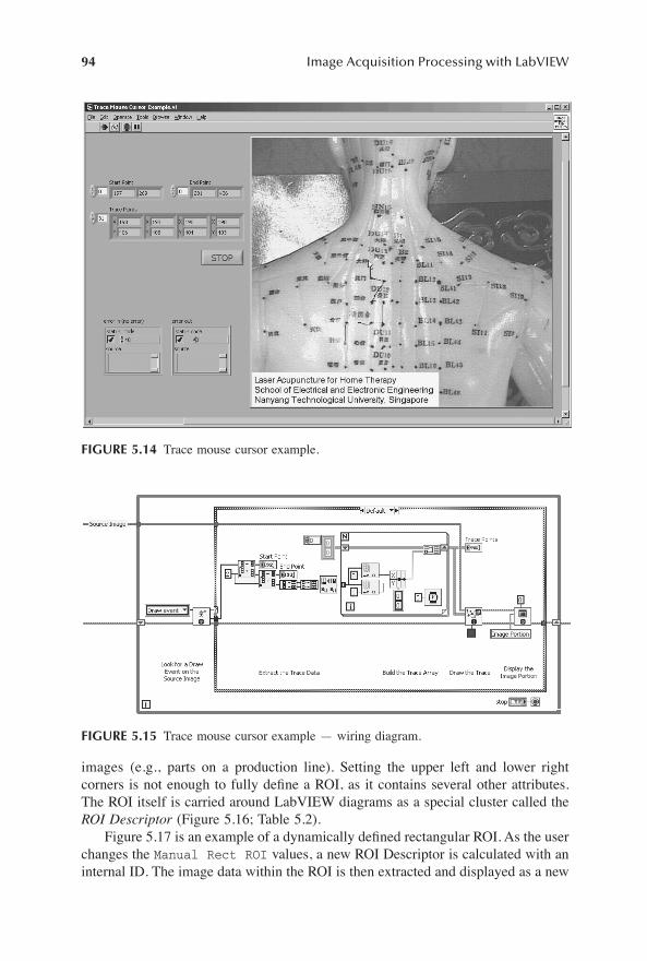
94
Image Acquisition Processing with LabVIEW
images (e.g., parts on a production line). Setting the upper left and lower rightcorners is not enough to fully deÞne a ROI, as it contains several other attributes.The ROI itself is carried around LabVIEW diagrams as a special cluster called the
ROI Descriptor
(Figure 5.16; Table 5.2). Figure 5.17 is an example of a dynamically deÞned rectangular ROI. As the user
changes the
Manual Rect ROI
values, a new ROI Descriptor is calculated with aninternal ID. The image data within the ROI is then extracted and displayed as a new
FIGURE 5.14
Trace mouse cursor example.
FIGURE 5.15
Trace mouse cursor example � wiring diagram.
1480_book.fm Page 94 Tuesday, June 24, 2003 11:35 AM

Image Processing
95
image (the example in Figure 5.18 uses the global rectangle as the coordinates, asthe type is a rectangle).
One often-useful application of dynamic ROI deÞnition is an
inspectionroutine
, which allows the user to pan and zoom a source image to locate features(Figure 5.19).
Although the wiring diagram in Figure 5.20 may look complicated, it is justan extension of previous examples. An event handler waits on the user pressingone of the inspection navigation buttons on the front panel and adjusts eitherthe window zoom or ROI descriptor to suit. The new values are then fed into
IMAQ WindZoom
and
IMAQ WindSetROI
and the inspection window isredrawn to reßect the changes.
FIGURE 5.16
The ROI descriptor.
TABLE 5.2
Item Description
Global rectangle The bounding box of the ROI � a rectangle whose bottom side is parallel to the bottom of the source image and encloses the complete ROI, irrespective of the ROI�s shape.
Contours Accurately deÞne the ROI with the following components:
ID:
SpeciÞes whether the ROI is considered to be within or without the deÞned shape. If the ID is external, the ROI is the complete image outside of the ROI coordinates and is not bound by the global rectangle.
Type:
SpeciÞes the contour shape (Point, Line, Rectangle, Oval, Polygon, Free, Broken Line, or Free Hand Line).
Coordinates:
SpeciÞes the list of contour points (e.g., the top left and bottom right points for a rectangle)
ROI
Global Rectangle
Source Image
Coordinates
Internal ID
1480_book.fm Page 95 Tuesday, June 24, 2003 11:35 AM

96
Image Acquisition Processing with LabVIEW
FIGURE 5.17
Manually building a rectangular ROI.
FIGURE 5.18
Manually building a rectangular ROI � wiring diagram.
FIGURE 5.19
Manual rectangular ROI application.
1480_book.fm Page 96 Tuesday, June 24, 2003 11:35 AM

Image Processing
97
FIGURE 5.20
Manual rectangular ROI application � wiring diagram.
1480_book.fm Page 97 Tuesday, June 24, 2003 11:35 AM

98
Image Acquisition Processing with LabVIEW
5.2 USER SOLUTION: DYNAMIC MICROSCOPY IN BRAIN RESEARCH
Michael Noll-Hussong and Arthur KonnerthLudwig-Maximilians-University MunichInstitute of PhysiologyPettenkofer Str. 12D - 80336 MuenchenGermanyTel +49 (0)89 5996 571/Fax +49 (0)89 5996 512Web site: http://www.neural.dee-mail: [email protected]
The study of nerve cells is today one of the most exciting challenges in research,especially because the biology of elementary processes like �learning� and �mem-ory� are not yet satisfactorily understood. Major progress toward a deeper under-standing of the brain�s functional mechanisms has been achieved with the develop-ment of imaging techniques, both macroscopic (e.g., employing positron-emissiontomography) and microscopic (e.g., confocal and multiphoton microscopy). Lattermode-locked laser-based microscopy techniques have made it possible to visualize,with a high temporal and spatial resolution, the dynamics of life processes at thesubcellular level, thus yielding new insights into the function of our brain on thecellular level. Of particular importance in this respect is the study of the changes inthe intracellular calcium concentration in nerve cells, given calcium�s involvementin the release of neurotransmitters and in memory processes. SpeciÞc ßuorescentindicator dyes can be introduced into living cells, which emit light of varyingwavelengths and intensities depending on the intracellular calcium concentration,thus making life processes accessible to direct visualization.
Our laboratory employs a range of microscopy systems of differing quality andfunctional characteristics. They are mostly integrated in electrophysiological work-benches, so that in the course of an experiment both imaging and conventionalelectrophysiological characterization of nerve cells are possible.
Addressing some fundamental questions of the physiology of our nervoussystem continually makes new demands on both the hardware (in its broadestmeaning) and the software used for investigations. The limitations encountered inour earlier studies made it very soon apparent that software development is anintegral component of our research. We soon reached the conclusion that wouldhave to construct modular software appropriate to our own needs and after anintensive search we came across the programming language LabVIEW, which, asfar as we were concerned, differed positively from its competitors in both itsorientation towards measurement techniques and its integration of hardware andsoftware components. Above all, the possibility of developing our own, checkableprogram codes and the capacity to adapt ßexibly to new demands spoke stronglyin favor of this development environment.
1480_book.fm Page 98 Tuesday, June 24, 2003 11:35 AM

Image Processing
99
As examples of our developments, we introduced program components foracquisition (
FastRecord
module) and analysis (
FastAnalysis
module) of imagedata obtained in the course of our brain research using laser microscopy. Theentire software suite was developed using LabVIEW 6i with IMAQ-Vision 6.0.5and the hardware employed included image capture cards (NI PCI-1408 and NIPCI-1409) and a DAQ card (NI PCI-6111E). The image acquisition module allowslossless recording of video data to a hard disk in real time, with analysis functionsbeing available simultaneously. A subsequent part of the program allows moredetailed analysis of the experimental data and prepares them for Þnal analysis inappropriate programs (
MS Excel
®
,
Wavemetric Igor
�). Further modules of oursoftware allow networking with other data sources (e.g., electrophysiologicalparameters, temperature, etc.) and the integration of control logic (e.g., controllingmicroscope motors). Other modules include procedures for image analysis instatic ßuorescence microscopy with an
auto-ROI
function and an
alignment
procedure based on structure recognition for
antidrift
correction in prolongedsequences of images.
5.2.1 P
ROGRAM
D
ESCRIPTION
The modules described were integrated in the program on the basis of a menu-drivenqueued state machine and thus could be executed directly via the GUI, or as indi-vidual menu items, whereby a uniform variable space deÞnition ensures dataexchange between the individual program components.
5.2.2 R
ECORDING
V
IDEO
S
EQUENCES
For high spatial and temporal resolution recording of the dynamic changes in theßuorescence characteristics of indicator dyes, a
recording
module (
FastRecord
)was developed to achieve the following:
� Lossless, real-time display of the biological object under investigation onthe computer monitor. In this case the (analogue) image delivered by themicroscope is processed directly by the computer program.
� Placement of ROIs over interesting regions of the image, interleaved withlossless, real-time display of
brightness-versus-time
courses.� Direct and lossless storage of image data on the hard disk.� Microscope control via the serial interface (e.g., laser shutter control,
control of the
z
-drive).� Communication with the electrophysiological module, for instance via
trigger connections (circuits) and networking of and with measurementdata from other sources.
� Simplicity and standardization of program operation, particularly withrespect to appropriateness for the task in hand, capacity for self-descrip-tion and conformity with expectation (in accordance with EN ISO 9241).
� Modular software concept with the option of expansion of the program�sfunctionality at any time.
1480_book.fm Page 99 Tuesday, June 24, 2003 11:35 AM

100
Image Acquisition Processing with LabVIEW
The procedure in the course of an experiment begins with the biological objectof interest (a single cell in a vital brain section) is displayed as a video image onthe PC monitor.
ROIs of any shape can be located at speciÞc positions in the image as desired.The mean brightness value of these ROIs can be displayed simultaneously besidethe live image as brightness-versus-time courses on the monitor. If required,pressing a key stores image sequences, theoretically of any desired length, withoutloss and in real time. The only limit to the recording duration is the storage capacityof the hard disk. The possibility for direct-to-disk storage is a major advance,since this circumvents the limitations inherent in the transient and nonpermanentstorage in the expensive RAM and thus allows direct and permanent storage ofdigital Þlms using the economic and theoretically unlimited capacity of the harddisk. In addition, it is possible to communicate with the various peripheral exper-imental instruments (laser shutter, microscope z-drive, etc.) and trigger connectionsallow data exchange with a so-called �patch-clamp� ampliÞer, so that the start ofan electrophysiological experiment can initiate the recording of an image sequenceand vice versa.
5.2.2.1 Analysis of Video Sequences
The primary aim of the FastRecord module is the comfortable and comprehensiveanalysis of image sequences of various formats (AVI, Bio-Rad�-PIC, BIN) obtainedusing FastRecord or other recording systems. The main focus thereby is the
capacity to produce (after deÞnition of the appropriate ROIs) brightness-versus-timecourses and to store the data in a format that can be read by conventional spreadsheetprograms (Figure 5.21).
The procedure for the calculation of the brightness-versus-time courses in cal-cium-imaging experiments is as follows: the mean brightness value (F) of a ROI is
FIGURE 5.21 Calculate brightness vs. time.
1480_book.fm Page 100 Tuesday, June 24, 2003 11:35 AM

Image Processing 101
calculated dynamically by summing the brightness values of all pixels within the ROI,dividing the sum by the number of pixels and rounding off mathematically to thenearest integer. The control brightness value (F0) for the ROI is calculated by summingthe individual images in the video sequence up to the point at which the evoked(electrophysiological) event commences, dividing the sum by the number of individualimages and then calculating the mean brightness for each ROI. After correcting (bysubtraction) both F and F0 for the background brightness (background ßuorescence),the quotient DF/F0 is obtained and displayed as the result of the analysis in thecorresponding curves, which can also be stored in a conventional spread-sheet format(e.g., Excel, Wavemetrics Igor) for Þnal analysis, if such is necessary.
5.2.3 SUMMARY
The program modules FastRecord and FastAnalysis represent a complete solu-tion for the recording and analysis of (analogue) ßuorescence data with high temporaland spatial resolution. FastRecord (Figure 5.22) offers PC-based, real-time andlossless recoding of image data, with the possibility of the simultaneous monitordisplay of the object under investigation as well as the graphical representation ofthe live ßuorescence values. The data obtained with FastRecord can be analyzedand prepared for presentation with FastAnalysis. The internal coordination andmodularity of the program assures simple and intuitive use, with the possibility ofexpansion and integration of further functions at any time. The use of the widespreadPC platform makes this program an economic alternative for carrying out imagingexperiments, the qualitative (functional appropriateness) and quantitative (processingspeed) characteristics are similar to those of commercially available imaging sys-tems. As our experience has shown, the modularity of the above programs allowsfor ßexible integration in larger applications that, as LabVIEW-based completesoftware, accompany the entire course of an experiment: managing, controlling,measuring and analyzing.
FIGURE 5.22 The FastRecord analysis module.
Wave-tableROIs superimposedon the live image
Background-correctedbrightness-versus-time graph
0
1480_book.fm Page 101 Tuesday, June 24, 2003 11:35 AM

102 Image Acquisition Processing with LabVIEW
5.3 CONNECTIVITY
The nature of image processing alters a PUI�s (pixel under investigation) value withrespect to its surrounding pixel values and perhaps the PUI itself. This process iscalled connectivity � it determines which pixels to use in the computation of newvalues. Most Vision Toolkit image processing and morphological routines are basedon 4, 6 or 8 pixel connectivity. Consider an image with its pixels referenced as theirposition within the image array:
Four-pixel connectivity concerns the image processing routine with the cardinal(i.e., North, East, South and West) pixels, so if the PUI is 23, then the connectivitypartners are 13, 22, 24 and 33:
00 01 02 03 04 05 06
10 11 12 13 14 15 16
20 21 22 23 24 25 26
30 31 32 33 34 35 36
40 41 42 43 44 45 46
00 01 02 03 04 05 06
10 11 12 13 14 15 16
20 21 22 23 24 25 26
30 31 32 33 34 35 36
40 41 42 43 44 45 46
1480_book.fm Page 102 Tuesday, June 24, 2003 11:35 AM

Image Processing 103
Six-pixel connectivity represents a hexagonal pixel layout, which can be simu-lated on a rectangular grid by shifting each second row by half a pixel:
If PUI were 23, its 6 pixel connectivity partners would be 12, 13, 22, 24, 32 and 33:
Eight-pixel connectivity concerns the image processing routine with the cardinaland subcardinal (i.e., North East, South East, South West and North West) pixels,so if the PUI is 23, then the connectivity partners are 12, 13, 14, 22, 24, 32, 33 and 34:
5.4 BASIC OPERATORS
Basic operators execute by performing a pixel-by-pixel transformation on the inten-sities throughout the source image(s) and function in two modes: with two sourceimages, or with one source image and a constant operator.
5.4.1 ADD (COMBINE)
Adding two source images is performed as simple matrix addition:
00 01 02 03 04 05 06 00 01 02 03 04 05 06
10 11 12 13 14 15 16 10 11 12 13 14 15 16
20 21 22 23 24 25 26 Þ 20 21 22 23 24 25 26
30 31 32 33 34 35 36 30 31 32 33 34 35 36
40 41 42 43 44 45 46 40 41 42 43 44 45 46
00 01 02 03 04 05 06
10 11 12 13 14 15 16
20 21 22 23 24 25 26
30 31 32 33 34 35 36
40 41 42 43 44 45 46
00 01 02 03 04 05 06
10 11 12 13 14 15 16
20 21 22 23 24 25 26
30 31 32 33 34 35 36
40 41 42 43 44 45 46
A1 A2 A3 B1 B2 B3 A1+B1 A2+B2 A3+B3
A4 A5 A6 + B4 B5 B6 = A4+B4 A5+B5 A6+B6
A7 A8 A9 B7 B8 B9 A7+B7 A8+B8 A9+B9
Source Image A Source Image B Combined Images
Dst x y SrcA x y SrcB x y, , ,( ) = ( ) + ( )
1480_book.fm Page 103 Tuesday, June 24, 2003 11:35 AM

104 Image Acquisition Processing with LabVIEW
Therefore, an example 3 ¥ 3 image combination would be implemented as follows:
As intensity values greater than 255 are forbidden in an 8-bit image (only valuesbetween 0 and 255 inclusive are permitted), any combined intensity values of 256or greater (shaded cells in the previous example) are clipped to 255 (white). There-fore, the true (distorted) output of the combination routine for this example is:
As you can see, the combined image�s intensity values are the added componentsand are therefore either larger than (hence brighter) or equal to that of the originalpixels. The example in Figure 5.23 was implemented with the code shown in Figure5.24, using IMAQ Add. IMAQ Add also allows for constant values to be added
to all image pixels � the constant input can be either positive or negative (Figure5.25). As you might expect, using a constant of 100, adds 100 intensity units to eachpixel of the source image (Figure 5.26).
122 127 125 122 0 111 244 127 236
190 120 123 + 187 130 113 = 377 250 236
115 178 160 117 180 167 232 358 327
Source Image A Source Image B Combined Images
122 127 125 122 0 111 244 127 236
190 120 123 + 187 130 113 = 255 250 236
115 178 160 117 180 167 232 255 255
Source Image A Source Image B Combined Images
FIGURE 5.23 (a) Source image A (b) Source image B (c) Combined images
1480_book.fm Page 104 Tuesday, June 24, 2003 11:35 AM

Image Processing 105
5.4.2 SUBTRACT (DIFFERENCE)
Subtraction is also performed as a simple matrix operation:
FIGURE 5.24 Add images � wiring diagram.
FIGURE 5.25 Add constant to image � wiring diagram.
FIGURE 5.26 Add constant to image.
A1 A2 A3 B1 B2 B3 A1-B1 A2-B2 A3-B3
A4 A5 A6 _ B4 B5 B6 = A4-B4 A5-B5 A6-B6
A7 A8 A9 B7 B8 B9 A7-B7 A8-B8 A9-B9
Source Image A Source Image B Combined Images
Dst x y SrcA x y SrcB x y, , ,( ) = ( ) - ( )
1480_book.fm Page 105 Tuesday, June 24, 2003 11:35 AM
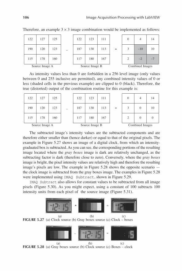
106 Image Acquisition Processing with LabVIEW
Therefore, an example 3 ¥ 3 image combination would be implemented as follows:
As intensity values less than 0 are forbidden in a 256 level image (only valuesbetween 0 and 255 inclusive are permitted), any combined intensity values of 0 orless (shaded cells in the previous example) are clipped to 0 (black). Therefore, thetrue (distorted) output of the combination routine for this example is:
The subtracted image�s intensity values are the subtracted components and aretherefore either smaller than (hence darker) or equal to that of the original pixels. Theexample in Figure 5.27 shows an image of a digital clock, from which an intensity-graduated box is subtracted. As you can see, the corresponding portions of the resultingimage located where the gray boxes image is dark are relatively unchanged, as thesubtracting factor is dark (therefore close to zero). Conversely, where the gray boxesimage is bright, the pixel intensity values are relatively high and therefore the resultingimage�s pixels are low. The example in Figure 5.28 shows the opposite scenario �the clock image is subtracted from the gray boxes image. The examples in Figure 5.28were implemented using IMAQ Subtract, shown in Figure 5.29.
IMAQ Subtract also allows for constant values to be subtracted from all imagepixels (Figure 5.30). As you might expect, using a constant of 100 subtracts 100intensity units from each pixel of the source image (Figure 5.31).
122 127 125 122 123 111 0 4 14
190 120 123 _ 187 130 113 = 3 �10 10
115 178 160 117 180 167 2 �2 �7
Source Image A Source Image B Combined Images
122 127 125 122 123 111 0 4 14
190 120 123 _ 187 130 113 = 3 0 10
115 178 160 117 180 167 2 0 0
Source Image A Source Image B Combined Images
(a) (b) (c)FIGURE 5.27 (a) Clock source (b) Gray boxes source (c) Clock � boxes
(a) (b) (c)FIGURE 5.28 (a) Gray boxes source (b) Clock source (c) Boxes � clock
1480_book.fm Page 106 Tuesday, June 24, 2003 11:35 AM

Image Processing 107
FIGURE 5.29 Subtract images � wiring diagram.
FIGURE 5.30 Subtract constant from image � wiring diagram.
FIGURE 5.31 Subtract constant from image.
1480_book.fm Page 107 Tuesday, June 24, 2003 11:35 AM

108 Image Acquisition Processing with LabVIEW
5.4.3 OTHER BASIC OPERATORS
5.4.4 AVERAGING
Image averaging is a well-tested method of minimizing acquired random imagenoise, hence increasing the signal-to-noise ratio (SNR). A common error when
Operator Description
Multiplies the pixels of two source images, or one source image with a constant. Be careful to match the source and destination images so that pixel intensity clipping does not occur (e.g., decrease the intensity range of the source images, or increase the destination image).
IMAQ Multiply
Divides the pixels of the Þrst source image with the pixels of the second source image or a constant.
IMAQ Divide
Computes a ratio between the two source images. Each pixel in Source Image A is multiplied by a constant and then divided by its equivalent Source Image B pixel. Unlike other basic operators, a temporary variable is used to perform this operation; so information is not lost due to compression
IMAQ MulDiv
Executes modulo division (remainder) of one image by another or an image by a constant
IMAQ ModuloFIGURE 5.32
Dst x y SrcA x y SrcB x y, , ,( ) = ( ) + ( )
Dst x ySrcA x y
SrcB x y,
,
,( ) = ( )
( )
Dst x yConst SrcA x y
SrcB x y,
,
,( ) =
( ){ }( )
Dst x y SrcA x y SrcB x y
SrcA x y
SrcB x y
, , ,
,
,
( ) = ( ) - ( ){ } ¥
( )( )
Í
ÎÍ
ú
ûú
1480_book.fm Page 108 Tuesday, June 24, 2003 11:35 AM

Image Processing 109
attempting image averaging is to add two images and then divide them by two,hoping for an image average (Figure 5.33). Although this technique will work whenthe added pixel values are not clipped to the maximum intensity, if the addition doesequal more than the maximum, compression will occur, as shown in Figure 5.34.
A better method is to scale down each of the source images before the addition(Figure 5.35) however, this reduces the dynamic range if rounding occurs, whichachieves the result shown in Figure 5.36.
FIGURE 5.33 Average images: The wrong way � wiring diagram.
FIGURE 5.34 (a) Source image A. (b) Source image B (c) The wrong way.
FIGURE 5.35 Average images: A better way � wiring diagram.
FIGURE 5.36 (a) Source image A (b) Source image B (c) A Better Way
1480_book.fm Page 109 Tuesday, June 24, 2003 11:35 AM

110 Image Acquisition Processing with LabVIEW
5.5 USER SOLUTION: IMAGE AVERAGING WITH LABVIEW
Don J. RothSenior Research EngineerNASA Glenn Research CenterCleveland, Ohioe-mail: [email protected]
Many data acquisition processes are besieged by noise, including those that areimage-based.1 Signal averaging is a simple and popular technique to reduce noiseor increase the signal-to-noise ratio (SNR). SNR is proportional to the square rootof the number of averages. Based on the circular buffer technique, the routines Ipresent allow the running image average of the most recent x number of images,with the number being continuously adjustable in real-time, without disruption ordiscontinuity of the averaging computation. The advantage of this is that you canmanage the trade-off between noise reduction and the amount of processing in thetime-domain during the test, if so desired. In other words, you can tune to, or �dialin,� the level of SNR desired while the experiment is running and actually see thein-situ effect on the image (Figure 5.37).
When dealing with continuous single shot measurements, a one-dimensionalarray is needed to hold the collection of point measurements. When dealing withwaveforms, a two-dimensional array is needed to hold the collection of one-dimen-sional waveforms. When dealing with images, a three-dimensional array is neededto hold the two-dimensional image frames. LabVIEW functions (such as initial-ize array, array subset and insert into array) need to be expanded to dealwith the different array sizes in each of the averaging schemes, as shown below.This is achieved by right clicking on the appropriate input terminal of the functionand selecting �add dimension� (Figure 5.38).
Image averaging was performed by indexing out the columns of the three-dimensional array and then using the LabVIEW Mean function (from the Mathe-matics, Probability and Statistics subfunction palette) on each column (one-dimen-sional array) within the three-dimensional array. To better visualize this, considereach image frame as a checkerboard of squares (pixels). Stack the checkerboardson top of each other. Now extract out the vertical columns at every location andcalculate the mean of each one. The result is a two-dimensional array of mean values(or an image average) (Figure 5.39).
The National Instruments Developer Zone shows an example running imageaverager using IMAQ Vision functions2 that operates somewhat differently than theone presented here. In the National Instruments example, after a speciÞed numberof images are averaged, the averaged image becomes the Þrst image for the new setof images to be averaged, whereas the routines presented here allow the runningimage average of the most recent x number of images.
1 Roth, Don J., LabVIEW Technical Resource, Vol. 8, No. 4, pp. 12�14.2 NI Developer Zone (http://zone.ni.com/) Example: Real-time Image Averaging.vi.
1480_book.fm Page 110 Tuesday, June 24, 2003 11:35 AM

Image Processing 111
FIGURE 5.37 Image averaging alternatives � Front panel example.
FIGURE 5.38 Image averaging alternatives � comparison with other averagers.
1480_book.fm Page 111 Tuesday, June 24, 2003 11:35 AM

112 Image Acquisition Processing with LabVIEW
In the example shown in Figure 5.37, a low-resolution sample image (89 ¥ 44pixels) plus simulated noise is provided as the input to demonstrate these routines.An unsigned 8-bit (U8) format with images scaled between 0 and 255 is used. Arraytransposition for the version using intensity graphs was necessary. A two-dimen-sional interpolation routine1 has been integrated to allow enlarging the image whileretaining the smoothing effect. The size of the active plotting area is adjusted interms of width and height in pixels based on the interpolation factor chosen (inter-polation factor numeric control will display when interpolation is selected in radiobutton control). The interpolation routine is only implemented in this example forthe intensity graph container but can easily be integrated into the examples usingIMAQ and Picture Control display containers.
For practical use of these routines, one would substitute NI-IMAQ routines thatperform continuous live image acquisitions from a CCD or other type of camera.The frame rate one obtains will be inversely proportional to the number of framesbeing averaged (as well as the physical size/number of pixels of the frames and sizeof intensity graph indicator). On a Compaq 1.5 GHz Xeon single processor-basedsystem, I was able to process about 50 fps with 10 frames averaged and a 1-msdelay in the while loop of the block diagram. Keep in mind a two-dimensional arrayof noise is calculated within each loop iteration while for an actual machine visionsituation, frame grabbing would be occurring instead and this will affect the trueframe rate achieved. A color table control routine is also included, allowing the userto modify the color table during acquisition, although a gray scale color table isprovided as the default.
FIGURE 5.39 Image averaging alternatives � how it works.
1 NI Developer Zone Example: 2D Interpolation demo.llb.
1480_book.fm Page 112 Tuesday, June 24, 2003 11:35 AM

Image Processing 113
5.6 OTHER TOOLS
Most of the other tools in the Image Processing palette of the Vision Toolkit speakfor themselves, but there are a few that are not completely intuitive.
5.6.1 SYMMETRY (MIRRORING AN IMAGE)
IMAQ Symmetry transforms an image to mirror along one or more axes (Figure5.40). Using IMAQ Symmetry is quite simple � all you need to deÞne is whichaxes to use (Figure 5.41).
FIGURE 5.40 Symmetry application.
FIGURE 5.41 Symmetry application � wiring diagram.
1480_book.fm Page 113 Tuesday, June 24, 2003 11:35 AM
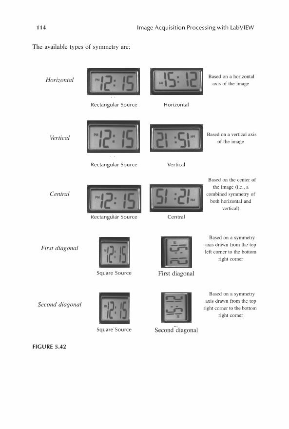
114 Image Acquisition Processing with LabVIEW
The available types of symmetry are:
Horizontal Based on a horizontal
axis of the image
Rectangular Source Horizontal
Vertical Based on a vertical axis
of the image
Rectangular Source Vertical
Central
Based on the center of the image (i.e., a
combined symmetry of both horizontal and
vertical)
Rectangular Source Central
First diagonal
Based on a symmetry axis drawn from the top left corner to the bottom
right corner
Square Source First diagonal
Second diagonal
Based on a symmetry axis drawn from the top
right corner to the bottom right corner
Square Source Second diagonal
FIGURE 5.42
1480_book.fm Page 114 Tuesday, June 24, 2003 11:35 AM

Image Processing 115
5.6.2 ROTATE
IMAQ Rotate allows you to rotate an image with single point ßoat accuracy (Figure5.43). This example (Figure 5.44) was achieved using a modiÞed version of ManualRectangular ROI Application.vi, discussed earlier.
As you can see, when image data is rotated, the image window itself does notrotate, leaving �blank� areas around the newly rotated section. The image data forthese areas is undeÞned, so IMAQ Rotate allows you to specify a replace value topaint them with. The replace value is speciÞed in intensity units between 0 and 255.
FIGURE 5.43 (a) Rectangular source. (b) Horizontal.
FIGURE 5.44 Rotate image application � wiring diagram.
1480_book.fm Page 115 Tuesday, June 24, 2003 11:35 AM
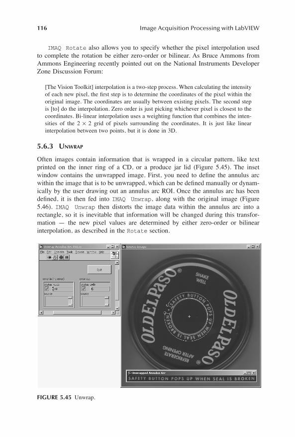
116 Image Acquisition Processing with LabVIEW
IMAQ Rotate also allows you to specify whether the pixel interpolation usedto complete the rotation be either zero-order or bilinear. As Bruce Ammons fromAmmons Engineering recently pointed out on the National Instruments DeveloperZone Discussion Forum:
[The Vision Toolkit] interpolation is a two-step process. When calculating the intensityof each new pixel, the Þrst step is to determine the coordinates of the pixel within theoriginal image. The coordinates are usually between existing pixels. The second stepis [to] do the interpolation. Zero order is just picking whichever pixel is closest to thecoordinates. Bi-linear interpolation uses a weighting function that combines the inten-sities of the 2 ¥ 2 grid of pixels surrounding the coordinates. It is just like linearinterpolation between two points, but it is done in 3D.
5.6.3 UNWRAP
Often images contain information that is wrapped in a circular pattern, like textprinted on the inner ring of a CD, or a produce jar lid (Figure 5.45). The insetwindow contains the unwrapped image. First, you need to deÞne the annulus arcwithin the image that is to be unwrapped, which can be deÞned manually or dynam-ically by the user drawing out an annulus arc ROI. Once the annulus arc has beendeÞned, it is then fed into IMAQ Unwrap, along with the original image (Figure5.46). IMAQ Unwrap then distorts the image data within the annulus arc into arectangle, so it is inevitable that information will be changed during this transfor-mation � the new pixel values are determined by either zero-order or bilinearinterpolation, as described in the Rotate section.
FIGURE 5.45 Unwrap.
1480_book.fm Page 116 Tuesday, June 24, 2003 11:35 AM

Image Processing 117
5.6.4 3D VIEW
A grayscale image has three dimensions � each pixel on a two-dimensional spatialplane has an intensity component, hence the third dimension. An often-useful methodof displaying these intensity maps is by using the Vision Toolkit�s 3D View, whereeach pixel�s intensity value is represented spatially (Figure 5.47). As you can see, thethree-dimensional representation is also artiÞcially shaded. This technique is achievedusing IMAQ 3D View (Figure 5.48). IMAQ 3D View is also useful to plot non-Visiontwo-dimensional arrays by Þrst converting them to IMAQ images (Figure 5.49).
The example in Figure 5.50 shows a two-dimensional array dataset plotted Þrstas a image (in a similar fashion to an intensity graph) and then as a 3D View image.
5.6.5 THRESHOLDING
Thresholding enables you to select ranges (often referred to as the threshold interval)of pixel intensity values in grayscale and color images, effectively compressing thevalues outside of the range to their respective extremes.
FIGURE 5.46 Unwrap � wiring diagram.
FIGURE 5.47 3D view.
I
I Range
I Range I Range
I RangeNew
Old Low
Old Low Old High
Old High
=<£ £>
Ï
ÌÔ
ÓÔ
0
255
1480_book.fm Page 117 Tuesday, June 24, 2003 11:35 AM

118 Image Acquisition Processing with LabVIEW
FIGURE 5.48 3D view � wiring diagram.
FIGURE 5.49 3D view: plot two-dimensional array � wiring diagram.
FIGURE 5.50 3D view � plot two-dimensional array.
1480_book.fm Page 118 Tuesday, June 24, 2003 11:35 AM

Image Processing 119
Consider a grayscale image:
Perhaps you are interested only in intensity values that fall within a particularrange, e.g., 140 and 175 inclusive. Performing a threshold operation on the previousimage would yield the following image:
You can also perform a binary threshold by suppressing the intensities outsideof the threshold interval to zero and highlighting those within the interval by settingtheir values to the maximum intensity values.
125 122 111 110 107
130 145 155 134 123
131 156 159 141 136
135 177 180 149 142
150 202 213 170 160
0 0 0 0 0
0 145 155 134 0
0 156 159 141 0
0 255 255 149 142
150 255 255 170 160
II Range I Range
Range I RangeNew
Old Low Old High
Low Old High
=< >
£ £ÏÌÓ
0
255
,
1480_book.fm Page 119 Tuesday, June 24, 2003 11:35 AM

120 Image Acquisition Processing with LabVIEW
Consider the previous image again. Performing a binary threshold using the sameinterval values of 140 and 175 yields:
For example, Figure 5.51 contains a barcode label. The label is relatively brightwhen compared with the rest of the image, so using a nonbinary threshold routinethat sets pixels with intensities higher than a value that is just lower than the labelwill achieve the result shown in Figure 5.52.
When used in binary mode, IMAQ Threshold also has a replace value input,so you can specify the intensity value to be used when the PUI�s value falls withinthe threshold interval (Figure 5.53). For example, setting a custom replace value of100 to the previous matrix image results in:
0 0 0 0 0
0 255 255 255 0
0 255 255 255 0
0 0 0 255 255
255 0 0 255 255
FIGURE 5.51 Power meter with barcode label.
1480_book.fm Page 120 Tuesday, June 24, 2003 11:35 AM

Image Processing 121
Applying the same replace value of 100 to the barcode label image above yieldsthe result in Figure 5.54.
0 0 0 0 0
0 100 100 100 0
0 100 100 100 0
0 0 0 100 100
100 0 0 100 100
FIGURE 5.52 Threshold example.
FIGURE 5.53 Threshold example � wiring diagram.
1480_book.fm Page 121 Tuesday, June 24, 2003 11:35 AM

122 Image Acquisition Processing with LabVIEW
5.6.6 EQUALIZATION
Equalization is similar to thresholding an image, except that it also spreads thethreshold interval intensities across the complete range permitted by the image type,redistributing the pixel values to linearize the accumulated histogram. Equalizationincreases the contrast of a particular range of intensities.
FIGURE 5.54 Threshold example � custom replace value.
FIGURE 5.55 Equalization example.
1480_book.fm Page 122 Tuesday, June 24, 2003 11:35 AM

Image Processing 123
For example, the image below contains a glare spot, where incident lighthas reßected from a glossy surface, creating a blind spot. Equalization can beused to enhance the image, effectively stretching the equalization range to coverthe complete intensity range, making it much easier to read the underlying text.The equalization example in Figure 5.55 was achieved using the code shown inFigure 5.56.
The equalization range is a cluster containing the elements described in Table5.3. Equalization can also be used to remove background data when an object�sintensities are very different from that of the background (Figure 5.57). Notice thatthe background is completely removed and the contrast of the leaves has beenincreased.
FIGURE 5.56 Equalization example � wiring diagram.
TABLE 5.3
Item DescriptionMinimum The minimum value is the smallest intensity to use during equalization. After the
equalization is complete, all pixel values that are less than or equal to the minimum in the original image are set to 0 for an 8-bit image. In 16-bit and ßoating-point images, these pixel values are set to the smallest pixel value found in the original image.
Maximum The maximum value is the highest intensity to use during equalization. After the equalization is complete, all pixel values that are greater than or equal to the maximum in the original image are set to 255 for an 8-bit image. In 16-bit and ßoating-point images, these pixel values are set to the largest pixel value found in the original image.
1480_book.fm Page 123 Tuesday, June 24, 2003 11:35 AM

124 Image Acquisition Processing with LabVIEW
FIGURE 5.57 Equalization example � removing a background.
1480_book.fm Page 124 Tuesday, June 24, 2003 11:35 AM

Image Processing 125
5.7 USER SOLUTION: QUICKTIME FOR LABVIEW
Christophe SalzmannSwiss Federal Institute of TechnologyLausanne, Switzerlande-mail: christophe.salzmann@epß.chWeb site: http://iawww.epß.ch
QuickTime is a free multimedia package from Apple (a fee-based Pro version isavailable, but not required to use the LabVIEW interface). It allows users toperform a wide variety of operations on images, movies and sounds, of which asubset has been provided to LabVIEW with the help of a CIN. As both QuickTimeand LabVIEW are platform independent, code written to exploit their strengths isalso cross-platform.
QuickTime can be seen as a set of APIs that supports a wide variety ofmultimedia tasks, implemented as a set of extensions under MacOS and DLLsunder Windows. Over the years, QuickTime has been extended to support manyof the current formats for compressing, transporting and storing images, videosand sounds and also handles 3D and VR objects, cubic panorama, MIDI music,etc. Many of the QuickTime functions are hardware accelerated, leveraging thegraphics processor as opposed to using the CPU for operations. Hardware accel-eration also permits applications to beneÞt from new hardware without requiringrecompilation of the source code.
5.7.1 QUICKTIME INTEGRATION TO LABVIEW
The output of many QuickTime operations results in an image displayed in the userinterface � the display of a given frame of a movie, for example. There are currentlytwo cross-platform methods of displaying images in LabVIEW: the use of an externalwindow and the use of the picture toolkit (although often popular, ActiveX solutionsare not cross-platform and therefore are not considered in this text). The externalwindow solution is similar to the IMAQ toolkit external window. The management ofthese external windows is not trivial and using the LabVIEW picture toolkit insteadcan alleviate many interfacing problems. A drawback of using the picture toolkit isthe display speed of the LabVIEW picture indicator, but as the speed of the graphicscard increases, this drawback tends not to be as noticed anymore. This solution alsosubstantially simpliÞes the internal management of the library, as there is no .c codeinvolved for the user interface, with native LabVIEW handling all aspects of it.
Great effort has been put in to this library, limiting the use of native QuickTimedialogs, replacing them with their LabVIEW equivalent, providing a greater ßexi-bility and familiarity to the user. The user can ask the library to provide the neededinformation in order to build a custom dialog, listing the image formats can berequested and displaying the results in a dialog ring, for example.
1480_book.fm Page 125 Tuesday, June 24, 2003 11:35 AM

126 Image Acquisition Processing with LabVIEW
5.7.1.1 QTLib: The QuickTime Library
In 1994, the ancestor of the QTLib existed for the Connectix (now Logitech) Quick-Cam, communicating through a serial link and displaying a grayscale grabbed imagein a LabVIEW intensity graph. Since then, it has evolved to support more camerasand frame grabbers and the integration of the picture toolkit to the standard versionof LabVIEW has permitted image display to be much faster. The current version ofQTLib adds QuickTime functions to manage grabbed images or other front panelelements, with the ability to save them as single image or as a movie.
The QTLib is implemented using a Fat-CIN, a technique that permits cross-platform capabilities by embedding multiple compiled codes into one Þle, with theappropriate platform speciÞc CIN automatically selected at run time using a dynamiccall (see Cross Platform CIN by Christophe Salzmann, LabVIEW TechnicalResource (LTR), Vol. 10, No. 1, 2002, at www.ltrpub.com for more informationconcerning Fat-CINs). There are six main usages for this library depicted by sixexamples VIs:
1. Reading single images2. Writing single images3. Reading movies (i.e., multiple images)4. Writing movies5. Video source frame grabbing6. Image transformation
5.7.1.2 Single Image Reading and Writing
QT_ImgOpen.vi (Figure 5.58) attempts to Þnd a QuickTime image importer thatsupports the Þles� encoding and will then decompress and return it in the ImageOut cluster. Then QT_QTImageToLVPict.vi converts the image to a LabVIEWpicture structure, appropriate to be drawn in a picture indicator. A warning isdisplayed if a suitable importer/decompressor was not found. The decompressionoperation can take some time and memory depending on the original image sizeand although QTLib will do its utmost to decompress the picture within the availablememory, it may fail. If this does occur, the image should be decompressed in parts,although this option is not yet available.
The WriteImage example takes an array of bytes representing an image andwrites them to the Þle speciÞed by the user. As QT_ImgSave.vi expects the imagean uncompressed 24-bit RGB image, you can convert a front panel element to thisformat using either PictToU8.vi or RefToU8.vi.
5.7.1.3 Reading Movies
The ReadMovie.vi (Figure 5.59) reads a selected movie frame by frame. Besidesthe native QuickTime movie format, various others are supported, including ani-mated GIF, ShockWave Flash and MPEG. Although some movie Þles can alsocontain more than one track (an audio, text or second video track for example),currently QTLib does not support them � only the primary video track is used.
1480_book.fm Page 126 Tuesday, June 24, 2003 11:35 AM

Image Processing 127
Also, it might be necessary for the software to drop frames or to extend the timeframes are displayed in order to play the movie in real-time, hence the Play at full speedbutton.
5.7.1.4 Writing Movies
Movie writing is similar to multiple sequential images writing (Figure 5.60). Cur-rently, only spatial compression is supported, as using a format with temporalcompression will trigger a new key frame for each frame. QT_MovieAddFrame.viadds an image to the created movie and the frame duration (expressed in the movietime base ticks, not in seconds) is speciÞed. Once all of the required frames areadded, the movie is closed with QT_MovieClose.vi.
5.7.1.5 Video Grabbing (Figure 5.61)
Video grabbing was the Þrst and only function of the initial version of QTLib andalthough the original version supported only one video input at a time, the currentversion supports up to 32 devices in parallel (Figure 5.61). QTLib has been suc-cessfully tested with USB, 1394 FireWire, serial and built-in digitizer boards. Asdescribed above, QTLib relies on video digitizer drivers to interface with imageacquisition hardware and although most of them respect the QuickTime standard,some do so only partially or not at all, so you should conÞrm your hardware willsupport the standard fully before purchasing it. Under Windows, the original QTLib
FIGURE 5.58 Using ReadImage and WriteImage.
FIGURE 5.59 Using ReadMovie.
1480_book.fm Page 127 Tuesday, June 24, 2003 11:35 AM

128 Image Acquisition Processing with LabVIEW
supported Video For Windows, which has many limitations including the lack ofconcurrent inputs. The use of Tim Molteno�s WinVDIG (see www.vdig.com formore information) alleviates this problem and permits the use of QuickTime standardAPIs across platforms.
A frame will be grabbed at the speciÞed size and returned as an image.QT_FGGrab.vi must be called as often has possible to keep up with the source�sframe rate (each frame has an ID associated to it, so you can see if a frame has beenmissed). It is also possible to modify various settings of the video inputs, such asbrightness and contrast, in real-time. Some video digitizer drivers have automaticsettings that overcome user control, while others may not provide control for all thestandard settings at all. The frame grabbing process occurs in parallel of otherLabVIEW tasks and then must stopped by calling QT_FGClose.vi (this VI alsoreleases all of the internal resources associated with the capture).
5.7.1.6 Image Transformation Functions
The image transformation function (Figure 5.62) applies one or more graphicaloperations (scale, rotation, skew, etc.) to a LabVIEW picture, or other LabVIEWfront panel elements that can be accessed through the Get Image method. Thisincludes picture indicators, graphs, charts, slides, strings, etc. For example, theTransformImage3.vi displays a 45û rotated thermometer. As picture indicators canreturn the mouse coordinates, it is possible to perform the reverse transformation to
FIGURE 5.60 Using WriteMovie.
FIGURE 5.61 Video grabbing example.
1480_book.fm Page 128 Tuesday, June 24, 2003 11:35 AM

Image Processing 129
map the mouse click back in the original coordinate. Then the appropriate action,like changing a slider value, can be taken to provide a real interactive solution.
5.7.1.7 Future Versions of QTLib
It is planned that QTLib will evolve in the future Þrst to keep pace with new releasesof QuickTime and LabVIEW and to add functions that could not be implementedin the current release of this library. The current version of the QTLib deals mostlywith Þles stored on the hard drive, although a future release will access memoryimage maps as well. Also, more transformations and effects will be added to theimage transformation VI.
5.7.1.8 For More Information
More detailed QuickTime information can be found at the Apple Web site(http://www.apple.com/quicktime) and an excellent introduction to QuickTime pro-gramming is Discovering Quicktime: An Introduction for Windows and MacintoshProgrammers, by George Towner and Apple Computer, published by Morgan Kauf-man, 1999.
FIGURE 5.62 Using TransformImage.
1480_book.fm Page 129 Tuesday, June 24, 2003 11:35 AM

130 Image Acquisition Processing with LabVIEW
5.8 FILTERS
Image Þlters are routines that either suppress or enhance data to meet a particularspeciÞed criterion. Typical Þlter uses include high contrast area enhancement, edgedetection and smoothing.
The two general types of Þlters that you may come across are linear (often referredto as a convolution) and nonlinear. Linear Þlters are designed to recalculate the valueof the PUI based on its original value and the values of those surrounding it. Thisconvolution often weights the effect surrounding pixels have on the PUI, usually withrespect to their distance from it (these weightings are reßected in the coefÞcients ofthe convolution kernel). An example convolution kernel is shown below:
The effect of this convolution kernel (hereafter referred to as the Þlter) is nothing.The recalculated value of the PUI is 1 time its original value, added to 0 times thevalues of those around it. A more useful example is:
This Þlter changes the value of the PUI to 1 time its original value, plus the sumof the North, East, South and West pixel values. Note: unless the intensity valuesof the used surrounding pixels are zero, the PUI�s value will become higher(brighter). If the PUI or its surrounding pixels� intensities sum to a value higherthan the maximum permitted for the image, intensity clipping will occur. A 256level grayscale image example using the above Þlter could be:
As an intensity value of 607 is forbidden in a 256 level image, the new PUIvalue will be clipped to 255 (white), which does not reßect the true nature of the
0 0 0
0 1 0
0 0 0
0 1 0
1 1 1
0 1 0
122 127 125 0 1 0
119 120 123 Æ 1 1 1 Æ 607
115 118 120 0 1 0
Image Data Filter New PUI Value
1480_book.fm Page 130 Tuesday, June 24, 2003 11:35 AM

Image Processing 131
Þlter. To avoid clipping, we can alter the previous kernel example to be a simpleaverager:
This Þlter assumes that the value of the original PUI is the most important(giving it a weighting of 1/2) and those at the North, East, South and West each haveequal importance of 1/8, so the same image example would be:
As all of the weightings of the Þlter add up to 1, there is no risk of the resultingPUI value exceeding the upper intensity limit of the pixel.
A 3 ¥ 3 kernel with positive elements has been used in the examples above, buta grid of practically any size and shape, with elements positive, zero or negativevalues can be deÞned as required by your application. If a kernel contains onlypositive elements, such as in the examples above, the effect is that of smoothing�low pass� Þlter. Conversely, if the elements are mixed positive and negative, asharpening �high pass� Þlter is achieved. The Vision Toolkit has a set of predeÞnedkernels for Gaussian, gradient, Laplacian and smoothing Þlters in standard sizes of3 ¥ 3, 5 ¥ 5 and 7 ¥ 7, although you can easily deÞne your own specialized Þltersof virtually any size.
5.8.1 USING FILTERS
You can use either the predeÞned Þlters built into the IMAQ Vision Toolkit, or createyour own for specialized applications. To apply a Þlter, you simply select (or deÞne)the appropriate kernel and then use IMAQ Convolute (Figure 5.63).
Connect your image source and kernel and IMAQ Convolute will do the rest.You may have also noticed the Divider (kernel sum) connector � it is a factor thatis applied to the sum of the obtained products. Usually, you can leave this terminalunwired (it defaults to zero), but if it is not equal to 0, the elements internal to thematrix are summed and then divided by this factor. This is not the same as normal-ization, where the output is scaled to fall between deÞned values (0 and 1 forexample), but is a raw operator.
0 1/8 0
1/8 1/2 1/8
0 1/8 0
122 127 125 0 1/8 0
119 120 123 Æ 1/8 1/2 1/8 Æ 121
115 118 120 0 1/8 0
Image Data Filter New PUI Value
1480_book.fm Page 131 Tuesday, June 24, 2003 11:35 AM
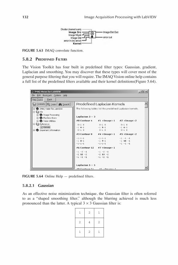
132 Image Acquisition Processing with LabVIEW
5.8.2 PREDEFINED FILTERS
The Vision Toolkit has four built in predeÞned Þlter types: Gaussian, gradient,Laplacian and smoothing. You may discover that these types will cover most of thegeneral purpose Þltering that you will require. The IMAQ Vision online help containsa full list of the predeÞned Þlters available and their kernel deÞnitions(Figure 5.64).
5.8.2.1 Gaussian
As an effective noise minimization technique, the Gaussian Þlter is often referredto as a �shaped smoothing Þlter,� although the blurring achieved is much lesspronounced than the latter. A typical 3 ¥ 3 Gaussian Þlter is:
FIGURE 5.63 IMAQ convolute function.
FIGURE 5.64 Online Help � predeÞned Þlters.
1 2 1
2 4 2
1 2 1
1480_book.fm Page 132 Tuesday, June 24, 2003 11:35 AM

Image Processing 133
Unlike a smoothing Þlter, the PUI weighting is greater than 1 and also greaterthan any of the neighboring pixels. This leads to a stronger inclination to the originalPUI value, which in turn promotes a much weaker smoothing effect. As you wouldexpect, a larger kernel grid invites the inßuence of pixels farther away, increasingthe blurring effect:
5.8.2.2 Gradient
Often one of the most interesting (and fun to play with!) Þlter families is the gradient.This Þlter is particularly useful when attempting to map intensity variations alonga speciÞc axis of the image. An example of a 45û gradient Þlter is:
This Þlter example seemingly �sweeps� through the image from the top rightcorner, highlighting variations in intensity, in the same manner as a Þrst-orderderivative. If you were to imagine this sweeping, as the Þlter detects an increase inintensity, it is marked lighter and decreases are marked darker (Figure 5.65).Although I have described this Þlter as having a �direction,� all noncumulative Þltersare purely directionless � the new image is built from artifacts of the source imageonly and therefore mathematically Þltering the pixels in differing directions (or ina random order) has no effect.
Another useful feature of the gradient Þlter is your ability to increase the apparentthickness of the edges detected. As you increase the size of your kernel, the thicknessalso increases (Figure 5.66).
As you can see from the 7 ¥ 7 kernel example, the image has become quitedistorted as the intensity gradients are more highlighted from the background, sothe value of increasing it to this level is questionable (depending on the softwareapplication�s purpose). In the previous example, the 5 ¥ 5 kernel looks to be a goodchoice and the effect of the Þlter is even more apparent when the negative of theimage is taken (Figure 5.67).
1 2 4 2 1
2 4 8 4 2
4 8 16 8 4
2 4 8 4 2
1 2 1 2 1
0 –1 –1
1 0 –1
1 1 0
1480_book.fm Page 133 Tuesday, June 24, 2003 11:35 AM

134 Image Acquisition Processing with LabVIEW
FIGURE 5.65 (a) Original shrub leaves image. (b) 45û Gradient Þltered image. (c) 125ûGradient Þltered image.
FIGURE 5.66 (a) 3 ¥ 3 45û Gradient Þltered image. (b) 5 ¥ 5 45û Gradient Þltered image.(c) 7 ¥ 7 45û Gradient Þltered image.
1480_book.fm Page 134 Tuesday, June 24, 2003 11:35 AM
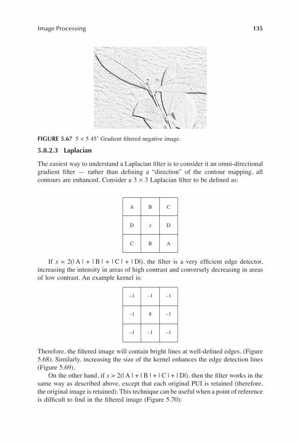
Image Processing 135
5.8.2.3 Laplacian
The easiest way to understand a Laplacian Þlter is to consider it an omni-directionalgradient Þlter � rather than deÞning a �direction� of the contour mapping, allcontours are enhanced. Consider a 3 ¥ 3 Laplacian Þlter to be deÞned as:
If x = 2(| A | + | B | + | C | + | D|), the Þlter is a very efÞcient edge detector,increasing the intensity in areas of high contrast and conversely decreasing in areasof low contrast. An example kernel is:
Therefore, the Þltered image will contain bright lines at well-deÞned edges, (Figure5.68). Similarly, increasing the size of the kernel enhances the edge detection lines(Figure 5.69).
On the other hand, if x > 2(| A | + | B | + | C | + | D|), then the Þlter works in thesame way as described above, except that each original PUI is retained (therefore,the original image is retained). This technique can be useful when a point of referenceis difÞcult to Þnd in the Þltered image (Figure 5.70):
FIGURE 5.67 5 ¥ 5 45û Gradient Þltered negative image.
A B C
D x D
C B A
�1 �1 �1
�1 8 �1
�1 �1 �1
1480_book.fm Page 135 Tuesday, June 24, 2003 11:35 AM

136 Image Acquisition Processing with LabVIEW
–1 –1 –1 –1 –1
–1 –1 –1 –1 –1
–1 –1 29 –1 –1
–1 –1 –1 –1 –1
–1 –1 –1 –1 –1
(a) (b)
FIGURE 5.68 (a) Original crushed terra cotta image. (b) 3x3 Laplacian Þltered image.
FIGURE 5.69 5 ¥ 5 Laplacian Þltered image.
1480_book.fm Page 136 Tuesday, June 24, 2003 11:35 AM

Image Processing 137
5.8.2.4 Smoothing
A smoothing Þlter is simply an averaging Þlter, blurring out features, details andobject shapes and is the most often used to, often inappropriately, minimize noise.The smoothing kernel assuages the variations in image intensity in the pixel neigh-boring the PUI. A simple smoothing kernel is:
As you can see, no weight is placed on the PUI � its calculated value is simplyan average of those around it, which all have the same weight, resulting in a blurredimage. As you would expect, a larger active kernel increases the blurring, as thedistant pixels begin to affect the resulting value of the PUI (Figure 5.71(a,b)).
5.8.3 CREATING YOUR OWN FILTER
Although the four general-purpose Þlter families provided with the Vision Toolkit arequite useful, they are by no means the only ones available. If you are unable to Þnd apre-deÞned Þlter to Þt your needs, designing a custom one is very easy. You can simplywire your kernel as a two-dimensional SGL array into IMAQ Convolute (Figure 5.72).
You can also use a Kernel string parser called IMAQ BuildKernel to constructa kernel array from a string. The code shown in Figure 5.73 yields the same resultas the example in Figure 5.72. This technique can be very useful when readingkernels from a text Þle, perhaps edited by a user not familiar with LabVIEW, orallowing Þlters to be altered as required after your application has been built,permitting you to distribute Þlters in a plug-in style.
It is good to model a Þlter before coding it, to get it right before openingLabVIEW. Find an excellent Web-based image convolution Þlter kernel utility at
(a) (b)
FIGURE 5.70 (a) Original crushed terra cotta image. (b) 5 ¥ 5 Laplacian Þltered image with PUI.
0 1 0
1 0 1
0 1 0
1480_book.fm Page 137 Tuesday, June 24, 2003 11:35 AM

138 Image Acquisition Processing with LabVIEW
http://www.cs.brown.edu/exploratory/research/applets/appletDescriptions/ÞlterKer-nel/home.html (Figure 5.74). This Java applet, developed by John F. Hughes and DaWoon Jung at Rhode Island�s Brown University, allows you to select an image,tweak standard kernels or deÞne your own and then view the effect your Þlter willhave. Using this utility could save you a lot of development time.
FIGURE 5.71 (a) Original King of Hearts image. (b) 5 ¥ 5 smoothing Þltered image.
FIGURE 5.72 Constant custom Þlter convolution kernel � wiring diagram.
FIGURE 5.73 Constant Þlter kernel parser � wiring diagram.
1480_book.fm Page 138 Tuesday, June 24, 2003 11:35 AM

Image Processing 139
FIGURE 5.74 Online Þlter kernel applet.
1480_book.fm Page 139 Tuesday, June 24, 2003 11:35 AM

1480_book.fm Page 140 Tuesday, June 24, 2003 11:35 AM

141
6
Morphology
When applied to vision, morphology (from the Greek word
morph,
meaning shapeor form) refers to the alteration of an image using computer routines. A more-common use for the term is the changing of an image in graduated steps (similar tothe �morphing� of an image of a baby to an adult), although this is a particular typeof morphology.
Occasionally, acquired images are not quite what we are looking for. They maycontain particle noise, or objects may have holes in them that we do not want ourvision routines noticing. When the acquired image is not suitable in these respects,then you need to morph.
6.1 SIMPLE MORPHOLOGY THEORY
Morphological operations are generally neighborhood based (the new value for thepixel under inspection (PUI) is determined from the values of its neighboring pixels).The two main types of binary morphological operations are
erosion
and
dilation
(other morphological operations exist, but are generally combinations of the two).Morphological operations are very similar to Þlters, except the kernels used aredependent on the original value of the PUI.
6.1.1 D
ILATION
Similar to the biological condition when referring to the human iris, dilation refersto the spatial expansion of an object with the potential of increasing its size, Þllingholes and connecting neighboring objects. Consider an image with the followingelements:
Simple dilation occurs when the following procedure is applied: if the PUI is1, then it retains its value; if it is 0, it becomes the logical OR of its cardinal (North,South, East and West) neighbors:
NW N NE
W
x
E
SW S SE
xx N E S W
otherwiseNewOld=
= $( ) =ÏÌÓ
1 1 1
0
, , , ,
1480_book.fm Page 141 Tuesday, June 24, 2003 11:35 AM

142
Image Acquisition Processing with LabVIEW
An example is shown below. Note that any PUIs with an original value of 1 areretained, small holes are Þlled and boundaries are retained:
6.1.2 E
ROSION
Similar to a small island in the middle of a river during water ßow, erosion wearsaway the edges of image features, decreasing its size, and potentially opening upholes in the object. Consider again the previous image with the following elements:
Simple erosion occurs when the following is applied: if the PUI is 0, then itretains its value; if it is 1 and all of its cardinal neighbors are also 1, then set thenew pixel value to 1 (otherwise set it to 0):
An erosion example is shown as follows:
6.1.3 C
LOSING
To �close� small holes and other background features in an image, all you need todo is Þrst dilate the source image, and then erode it:
Dilate
Þ
NW N NE
W
x
E
SW S SE
Erode
Þ
xx
x N E S WNewOld
Old
==
� ( ) =ÏÌÓ
0 0
1 1= 1 and , , ,
1480_book.fm Page 142 Tuesday, June 24, 2003 11:35 AM

Morphology
143
Although performing two seemingly opposite morphs on the source image maysuggest that it will result in the destination image being the same as the source, thisis not the case. Original image data is lost on executing the Þrst operation, and hencethe original image cannot be recovered.
As you can see, the small inner holes were Þlled, as was a portion of the upperinlet.
6.1.4 O
PENING
Opening an image (expanding holes and other background features in an image)requires the opposite sequence to closing: Þrst erode the source image, and thendilate it:
The opened image may not look much like its source, although the thinnerportions of the object have been successfully opened, and only the bulk area remains.
6.1.5 N
ONBINARY
M
ORPHOLOGY
Although the simplest method of morphology is to Þrst threshold an image, creatinga binary image (a pixel is either light or dark � there is no in-between), othermethods exist such as gray and color morphology.
Gray morphology is achieved by considering each of the neighboring colors asbinary couples, and performing binary morphology between them. This process is
Dilate Erode
Þ Þ
Erode Dilate
Þ Þ
I Erode Dilate IClosed Source= ( ){ }
I Dilate Erode IOpened Source= ( ){ }
1480_book.fm Page 143 Tuesday, June 24, 2003 11:35 AM

144
Image Acquisition Processing with LabVIEW
repeated for
n
colors
�1 (i.e., the number of color neighboring couples), and then thesemorphed images are weighted back using their respective gray levels (each morphedbinary is typically promoted to the next highest gray level) and recombined into animage with
n
colors
�1 colors.
6.2 PRACTICAL MORPHOLOGY
Simple dilation, erosion, opening and closing can be easily achieved using either
IMAQ Morphology
or
IMAQ GrayMorphology
1
(Figure 6.1).The morphological function performed on the source image in Figure 6.1 was
performed using the code shown in Figure 6.2. Similarly, both opening and closing
can be achieved using the same VIs. As you can see in Figure 6.3, the openingroutine discards the small specular objects around the main object, whereas theclosing routine attempts to include the specular data to the east of the circle,effectively closing the spaces between the solid object and close outlying objects(Figure 6.4)
FIGURE 6.1
Simple morphology � erosion and dilation.
1
These vision routines presume that the object of an image is the brightest section, and the backgroundis the darkest; therefore, you may need to invert an image before attempting practical morphology.
FIGURE 6.2
Simple morphology: erosion and dilation � wiring diagram.
1480_book.fm Page 144 Tuesday, June 24, 2003 11:35 AM

Morphology
145
6.3 THE STRUCTURING ELEMENT
You can change the way the morphing routines transform an image by deÞning acustom
structuring element
. A structuring element is a binary mask that deÞneswhich neighboring pixels are considered when performing a morphological func-tion. The previous examples have been executed using a standard structuringelement:
FIGURE 6.3
Simple morphology � opening and closing.
FIGURE 6.4
Simple morphology: opening and closing � wiring diagram.
0 1 0
1 1 1
0 1 0
1480_book.fm Page 145 Tuesday, June 24, 2003 11:35 AM
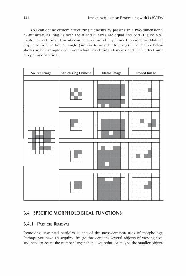
146
Image Acquisition Processing with LabVIEW
You can deÞne custom structuring elements by passing in a two-dimensional32-bit array, as long as both the
n
and
m
sizes are equal and odd (Figure 6.5).Custom structuring elements can be very useful if you need to erode or dilate anobject from a particular angle (similar to angular Þltering). The matrix belowshows some examples of nonstandard structuring elements and their effect on amorphing operation.
6.4 SPECIFIC MORPHOLOGICAL FUNCTIONS
6.4.1 P
ARTICLE
R
EMOVAL
Removing unwanted particles is one of the most-common uses of morphology.Perhaps you have an acquired image that contains several objects of varying size,and need to count the number larger than a set point, or maybe the smaller objects
Source Image Structuring Element Dilated Image Eroded Image
1480_book.fm Page 146 Tuesday, June 24, 2003 11:35 AM

Morphology
147
will be discarded in a future production process, so should be ignored when buildingstatistical datasets.
IMAQ Filter Particle
is a very powerful VI in the VisionToolkit, which can be used for particle removal (Figure 6.6).
The Selection Values input is an array of clusters (Figure 6.7).The cluster deÞnesthe particle removal method (Table 6.1). The cluster is placed inside an array, andit permits multiple selection criterion to be deÞned. For example, you can performa particle removal that removes particles smaller than a speciÞc area, and those thatdo not conÞrm to a deÞned circularity, all within one VI (each particle removal stepexecutes in the same order as they are deÞned in the array).
A simple particle removal example is shown in Figure 6.8. In this example, theselection values array has only one element, with the cluster values deÞned as shownin Table 6.2. This was achieved using the code shown in Figure 6.9.
IMAQ BasicParticle
was used to determine the number of particles bothbefore and after the routine was completed. This VI is also useful when you areinitially determining the lower and upper values of the particle removal, as it alsoreturns an array that describes each of the particles detected (Figure 6.10). Theclusters return the pixel and calibrated areas (if calibration data exists) of each
detected particle, and its global rectangle (a rectangle that is parallel to the image�sborder and bounds the particle) (Figure 6.11).
6.4.2 F
ILLING
P
ARTICLE
H
OLES
Once you have removed any unwanted particles from the image, a good next stepis to Þll any holes in the images objects. Filling holes gives you solid image objects,which are more easily counted and measured (Figure 6.12).
IMAQ FillHole
acceptsbinary source images and changes the intensity values of any detected hole pixels to 1
FIGURE 6.5
Custom structuring element.
FIGURE 6.6
IMAQ Filter Particle
.
1480_book.fm Page 147 Tuesday, June 24, 2003 11:35 AM

148
Image Acquisition Processing with LabVIEW
(maximum intensity in a binary image). As seen in Figure 6.12, holes ttouching the edgeof the image are not Þlled, as it is impossible from the information provided to determinewhether they are holes or outside edges of irregularly shaped objects (Figure 6.13).
6.4.3 D
ISTANCE
C
ONTOURING
6.4.3.1 IMAQ Distance
Distance contouring is a neat function that visually maps the relative distance of apixel to its border�s edge. More strictly, distance contouring encodes a pixel valueof a particle as a function of the location of that pixel in relation to the distance tothe border of the particle. As you might expect, the source image must have been createdwith a border size of at least 1, and be an 8-bit image. Using
IMAQ Distance
, you canalso deÞne whether the routine uses a square or hexagonal pixel frame during thetransformation (Figure 6.14).
IMAQ Distance
is a very simple VI to use, as shown in Figure 6.15.
FIGURE 6.7
Morphology selection values cluster.
TABLE 6.1Selection Values Cluster
Cluster Item Description
Parameter DeÞnes the type of removal to be performed. Examples include
area, center of mass position, segment lengths, orientation
and
circularity
.Lower value The lower value which the parameter is based on. For example, when using an
area
parameter, the lower value is the smallest area on which to base the area removal routine; if using the include interval, particles smaller than the lower value are discarded.
Upper value The upper value which the parameter is based on. For example, when using an area parameter, the upper value is the largest area on which to base the area removal routine; if using the include interval, particles larger than the lower value are discarded.
Interval Whether to include the range between the upper and lower values, or exclude them when applying the
parameter
routine.
1480_book.fm Page 148 Tuesday, June 24, 2003 11:35 AM

Morphology
149
FIGURE 6.8
Particle removal.
TABLE 6.2Selection Values Cluster Example
Cluster Item Value Description
Parameter Area (pixels) Particle removal is based on the pixel area of detected particles (a calibrated area routine is also available)
Lower value 0.00Upper value 3000.00Interval Include Process the routine using the values between and including
the lower (zero pixels area) and upper (3000 pixels area) values
FIGURE 6.9
Particle removal � wiring diagram.
1480_book.fm Page 149 Tuesday, June 24, 2003 11:35 AM

150
Image Acquisition Processing with LabVIEW
6.4.3.2 IMAQ Danielsson
Although
IMAQ Distance
is useful for fast distance contouring, as seen fromFigure 6.14, the transform is far from accurate. A much more accurate, yet slowerapproach is to use
IMAQ Danielsson
(Figure 6.16). The
Danielsson distance map
algorithm, which was devised by Erik Danielsson, is based on the Euclidian distancemap. The map values are coordinates giving the
x
and
y
distances to the nearestpoint on the boundary, and are stored as complex valued pixels. Then the absolutefunction is used to transform these into the radial distance. More information aboutthe Danielsson distance map can be found in the paper �Distance Maps for BoundaryDetect ion and Par t ic le Rebui lding,� by Frédér ique and Lefebvre(http://www.ici.ro/ici/revista/sic97_3/GUY.html).
IMAQ Danielsson
is eveneasier to use than
IMAQ Distance
, as it is not necessary to specify whether touse square or hexagonal pixel frames (Figure 6.17).
FIGURE 6.10
IMAQ basic particle basic reports.
FIGURE 6.11
The global rectangle.
Global Rectangle
Source Image
Detected Particle
1480_book.fm Page 150 Tuesday, June 24, 2003 11:35 AM

Morphology
151
6.4.4 B
ORDER
R
EJECTION
Objects are often intersected by the image border, and are therefore difÞcult tocharacterize. Figure 6.18 includes an irregular object that could be confused with acircle, and two circles with faults that could be assumed as holes. Although assump-
FIGURE 6.12
Fill holes.
FIGURE 6.13
Fill holes � wiring diagram.
1480_book.fm Page 151 Tuesday, June 24, 2003 11:35 AM

152
Image Acquisition Processing with LabVIEW
FIGURE 6.14
Distance example.
FIGURE 6.15
Distance example � wiring diagram.
FIGURE 6.16
Danielsson example.
Source Hexagon Square
1480_book.fm Page 152 Tuesday, June 24, 2003 11:35 AM

Morphology
153
tions could be made to extend these fragments to full objects, not enough informationis present to accurately do so. This is why it is often appropriate to ignore any objectsthat are touching the image border, and perhaps consider them in future acquiredframes if the objects are moving.
The example shown in Figure 6.19 counts and labels the total number of objectsthat are wholly within the image. This was achieved using
IMAQ RejectBorder
,which has very few inputs: the source and destination image data spaces and theconnectivity (Figure 6.20).
6.4.5 F
INDING
AND
C
LASSIFYING
CIRCULAR OBJECTS
If the image contains circular objects that you want to classify, a very simple VI touse is IMAQ Find Circles. This VI will search for circles in the image and return
FIGURE 6.17 Danielsson example � wiring diagram.
FIGURE 6.18 Irregular objects touching the image border.
FIGURE 6.19 Border rejection example.
Image Border
Irregular Object
Object with aSection Missing
Object witha Hole
1480_book.fm Page 153 Tuesday, June 24, 2003 11:35 AM

154 Image Acquisition Processing with LabVIEW
all sorts of information about them, including the number of circles detected, andtheir respective center positions, radii and calculated area (Figure 6.21).
IMAQ Find Circles uses a Danielsson distance map to determine the radiusof each object and can also separate perceived overlapping circles. This is imple-mented using the code shown in Figure 6.22, and an example application is shownin Figure 6.23.
FIGURE 6.20 Find and classify circular objects � wiring diagram.
FIGURE 6.21 Find and classify circular objects .
FIGURE 6.22 Find and classify circular objects � wiring diagram.
1480_book.fm Page 154 Tuesday, June 24, 2003 11:35 AM

Morphology 155
Detected circles with radii between 30 and 40 pixels are included in the search; therefore, the smaller objects are disregarded.
Detected circles with radii between 10 and 30 pixels are included in the search; therefore, the larger objects are disregarded.
All of the circular objects are detected, as the search radii range is between 10 and 40 pixels. Note that the two small circles that were overlapping have been separated and characterized correctly.
Decreasing the lower limit of the radii search range to 1 pixel has detected two extra circles, both of which are actually noise in the image.
FIGURE 6.23
1480_book.fm Page 155 Tuesday, June 24, 2003 11:35 AM

156 Image Acquisition Processing with LabVIEW
6.4.6 PARTICLE SEPARATION
If two or more particles are touching or overlapping in an image, you can separate themusing IMAQ Separation. This VI performs a series of morphological erosions andthen reconstructs the image based on any created object divisions (Figure 6.24).
If an isthmus is broken or removed during the erosion process, the particlesare reconstructed without the isthmus. The reconstructed particles generally havethe same size as their respective initial particles, although this can fail when thenumber of erosions is high. IMAQ Separation is simple to use (note that themajority of the code in Figure 6.25 is to label each particle with a number).
If the number of erosions is small, IMAQ BasicParticle can be used todetermine the area of the newly separated particles; if the number of erosions ishigh, particle counts andglobal rectangle measurements are generally still quiteaccurate.
FIGURE 6.24 Particle separation example.
FIGURE 6.25 Particle separation example � wiring diagram.
1480_book.fm Page 156 Tuesday, June 24, 2003 11:35 AM

Morphology 157
6.5 CASE STUDY: FIND AND CLASSIFY IRREGULAR OBJECTS
A user recently posted a question on the National Instruments Developers� Zonediscussion forum:
I want to read a barcode that is [a small part of] a big image�. I am not able to readthe barcode as I have to give the correct ROI, which in my case has to be setdynamically.
The image in question was indeed large (1600 ¥ 1400 pixels), and the positionthat the barcode label was attached to the object was undeÞned. The approach usedwas divided into several steps, as shown in Table 6.3.
The VI was coded as shown in Figure 6.26. As IMAQ BasicParticle wasused to Þnd the bounding rectangle of the barcode label, the position of the label(as long as it was completely within the source image) was irrelevant (Figure6.27).
TABLE 6.3
VI FunctionIMAQ Resample Resize the image to 800 ¥ 600 pixels (the extra image
information was not required)IMAQ Threshold Threshold the image to highlight the label (it is one of
the brightest areas of the source image)IMAQ FillHole Fill any holes in the objects that remain (including the
black numbers and bars of the actual barcode)IMAQ Particle Filter Filter out any objects that have calibrated areas outside
of a deÞned range (this removes objects that do not have the same area as the barcode label)
IMAQ BasicParticle Find the Bounding Rectangle of the remaining object (the barcode label)
IMAQ Extract Extract the barcode label from the source imageIMAQ Read Barcode Parse the label for its value
FIGURE 6.26 Search for label and read barcode � wiring diagram.
1480_book.fm Page 157 Tuesday, June 24, 2003 11:35 AM

158 Image Acquisition Processing with LabVIEW
FIGURE 6.27 Search for label and read barcode.
1480_book.fm Page 158 Tuesday, June 24, 2003 11:35 AM

Morphology 159
6.6 USER SOLUTION: DIGITAL IMAGING AND COMMUNICATIONS IN MEDICINE (DICOM) FOR LABVIEW
Chris ReedDevelopment EngineerDepartment of Medical PhysicsRoyal Perth Hospital, AustraliaTel +61-8-9224-2953/Fax +61-8-9224-1138e-mail: [email protected]
The DICOM Encoder is at the center of a suite of software tools designed for theacquisition and analysis of ultrasound images in cardiovascular research, althoughit can be easily adapted to any of the standard medical areas such as angiographyand nuclear medicine. The main function of the DICOM Encoder is to convert ananalog video signal (PAL or NTSC) into a DICOM-compatible digital Þle and logit to disk. This is achieved in real-time and at the full frame rate of the incomingvideo signal, using the National Instruments range of image acquisition cards. Thehighest quality signal is captured directly from the ultrasound machine, althoughprevious studies on analog tapes can also be converted into digital DICOM formatthrough a standard VCR. If required, a PCI expansion box can be used with a laptopto provide a portable solution for video capture and archiving. A standard DAQ cardcan also be used to acquire physiological data (e.g., pressure), but the latest approachis to display this information in the actual image, providing a cheaper solutionwithout being concerned with synchronizing the acquired data with the videosequence.
The DICOM Encoder was developed to bridge the gap between the old analogtechnology and the new digital world of DICOM and overcomes the followingproblems:
� Hardware limitations: ultrasound machines typically have limited ram andhard drive capacity, unlike that of a high-performance pc, greatly extend-ing the available capture time of individual studies from a minute or twoto over half an hour or more. The accessing and automated archiving ofsuch large Þles is also much quicker and easier.
� Pulse wave (pw) mode: common ultrasound machines are unable to cap-ture and store continuous video in pw mode. As the dicom softwarecaptures the raw signal directly from the ultrasound probe, there are nolimitations on which mode the ultrasound unit is in. This feature is essen-tial for techniques including blood ßow analysis, which requires the dop-pler velocity trace.
� Consistent frame rates: the dicom system can guarantee 25 fps (pal), 30fps (ntsc) sustained capture rates, regardless of image compression or size.
� Image resolution/quality: using the �camera� quality analog output fromthe ultrasound machines, it is possible to greatly improve the quality of
1480_book.fm Page 159 Tuesday, June 24, 2003 11:35 AM

160 Image Acquisition Processing with LabVIEW
the digital image stored to Þle as opposed to the traditional analog tape,currently considered the �gold standard.�
� File formats: the dicom Þle format offers random access to the data, aworldwide standard Þle format and no image quality degradation over time.
6.6.1 THE HARDWARE
Figure 6.28 shows the hardware system overview.
6.6.2 THE SOFTWARE
DICOM was developed using a number of software tools:
� LabVIEW 6.1� IMAQ Vision Toolkit 6.0� Intel JPEG Library v1.51� DicomObjects 4.1� LabVIEW Image Library v1.01
After a system frame rate hardware/software test is completed, the user is thenallowed to acquire a study. Relevant study information (patient name, hardware,medical details, etc) have already been entered and encoded in the DICOM HeaderInterface (Figure 6.29).
The Settings interface allows the user to select the image format (color/mono-chrome) and has other default settings that are used by other modules in the program(Figure 6.30).
Initially, the user can perform an auto exposure on the image to set the optimalbrightness level, or can manually adjust the white/black reference levels. When theRecord button is pressed, acquired images are encoded into JPEG format, displayedand logged to disk simultaneously. The study details (Þle size, number of frames,frame size and study length) are also updated. When the study is complete, the usercan calibrate the image to convert screen pixels into a known length, velocity or anyother physiological signal (pressure, ECG, etc.). All this information is embeddedinto the Þle according to the format of the DICOM Standard.
Although typical commercial medical devices may occasionally store a Þleas large as 20 MB, they are generally only a couple of megabytes. However,research studies can typically last up to 20 minutes, thus creating a single dataÞle that could be in excess of 1.2 GB. Standard DICOM Þles of this size cantake several minutes to save after acquisition, so a specialized fast save formatwas developed, allowing a study of any size to be ready for review immediatelyafter the acquisition is completed. This new format is not strictly DICOM com-patible, although a conversion utility is provided to convert the fast save data tothe standard format.
Any DICOM Þles can be read and displayed in the Edit/Review Interface,and all the study information is displayed in a separate window when the Detailsbutton is pressed. A horizontal pointer slide is used to display any frame in the
1480_book.fm Page 160 Tuesday, June 24, 2003 11:35 AM
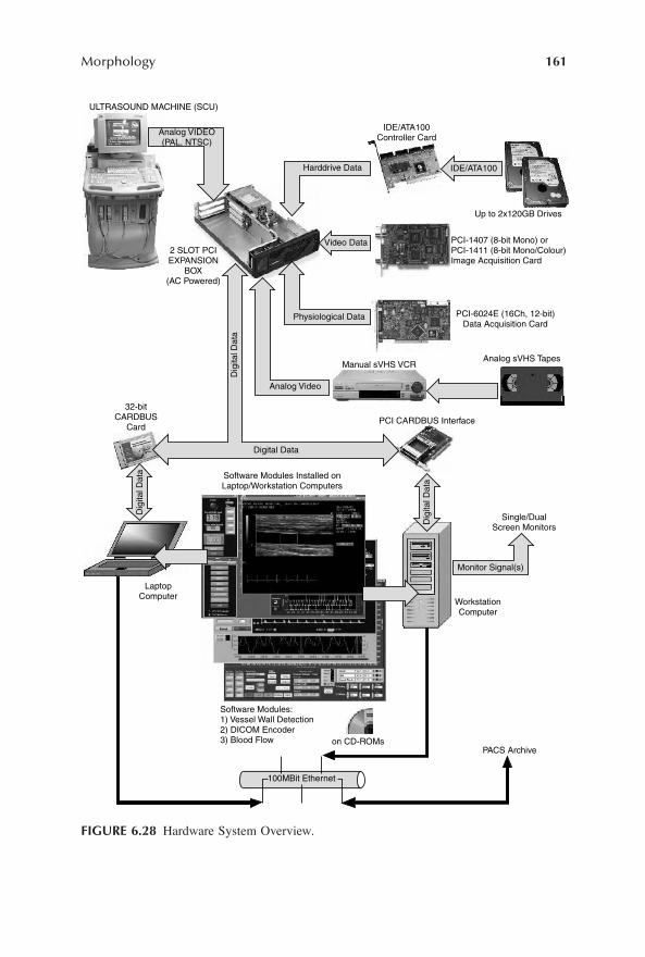
Morphology 161
FIGURE 6.28 Hardware System Overview.
ULTRASOUND MACHINE (SCU)
Analog VIDEO(PAL, NTSC)
IDE/ATA100Controller Card
2 SLOT PCIEXPANSION
BOX(AC Powered)
Up to 2x120GB Drives
PCI-1407 (8-bit Mono) orPCI-1411 (8-bit Mono/Colour)Image Acquisition Card
PCI-6024E (16Ch, 12-bit)Data Acquisition Card
Manual sVHS VCRAnalog sVHS Tapes
32-bitCARDBUS
CardPCI CARDBUS Interface
Single/DualScreen Monitors
Software Modules Installed onLaptop/Workstation Computers
LaptopComputer
WorkstationComputer
Software Modules:1) Vessel Wall Detection2) DICOM Encoder3) Blood Flow on CD-ROMs
PACS Archive
Harddrive Data IDE/ATA100
Video Data
Physiological Data
Digital Data
Dig
ital D
ata
Analog Video
Dig
ital D
ata
Dig
ital D
ata
Monitor Signal(s)
100MBit Ethernet
1480_book.fm Page 161 Tuesday, June 24, 2003 11:35 AM

162
Image Acquisition Processing with LabVIEW
study, and an XY Graph displays the length of the study and markers for the timethe user pressed paused during acquisition. It is also used to mark the start andend of a sequence, which can be converted into an MPEG or AVI movie usingany of the installed system codecs. The user also has a range of VCR-style buttonsto review the study, with the
Play Rate
control allowing rates up to eight timesnormal speed. By changing the
Search Mode
from
Normal
to
Index
, the user caninstantly jump to the start of each session using the pause markers as a reference(Figure 6.31).
FIGURE 6.29
The
Settings
dialog box.
FIGURE 6.30
The
Acquire
user interface.
1480_C06.fm Page 162 Tuesday, June 24, 2003 4:02 PM

Morphology 163
6.6.3 SUMMARY
The major lesson learned from developing this package was to use establishedsoftware wherever possible to reduce development time. Using LabVIEW and IMAQsimpliÞed development and provided a range of advanced features that linked thehardware and software together, albeit at a high cost. Using these two tools madethis part of the software relatively easy to accomplish. The most difÞcult aspect ofthe development was the understanding and interfacing to the DICOM Standard,which was achieved using an ActiveX toolkit and has so far proved remarkablyrobust in the latest version of LabVIEW, considering the problems in earlier versions.
6.6.4 ACKNOWLEDGMENTS
� Dr. David Harvey from Medical Connections, for his DicomObjectsActiveX component, which handles all aspects of the DICOM Standardand his expert knowledge of the Þeld (see www.medicalconnections.co.ukfor more information).
� Richard Weatherill for his help in developing the Encoder software. � Holger Lehnich from the Martin-Luther-University Halle-Wittenberg
Medical Faculty for the use of his Motion JPEG Encoder and its furtherdevelopment for the DICOM application.
� Icon Technologies for their LabVIEW Image Library and valued supportas a National Instruments Select Integrator/Alliance Member. See theirwebsite at http://www.icon-tech.com.au for more information.
FIGURE 6.31 The Edit and Review user interface.
1480_book.fm Page 163 Tuesday, June 24, 2003 11:35 AM

1480_book.fm Page 164 Tuesday, June 24, 2003 11:35 AM

165
7
Image Analysis
Image analysis is a nondestructive method of computing measurements and statisticsbased on the intensity values of an image�s pixels, and their respective spatial locationwithin that image. Analyzing an image can give you insight to objects that it mightcontain, and allows you to perform measurements on those objects, or veriÞcationon their presence.
7.1 SEARCHING AND IDENTIFYING (PATTERN MATCHING)
If you are looking for a particular object within an image,
IMAQ CountObjects
is not really going to help you, unless you speciÞcally know that theonly objects in your images are the type that you are looking for. What you willneed is a template of what you are looking for, a list of degrees of freedom thatyou are willing to accept, and a routine to search for the template within theacquired image.
Consider the image of a PCB shown in Figure 7.1. This PCB design has threesimilar circuits laid out on the board in parallel. If you were looking for theexistence of a particular component, an image of that component (or a suitableportion of it) would form your search template (Figure 7.2). By performing agrayscale pattern match, you are able to identify possible instances of the template(Figure 7.3).
FIGURE 7.1
Sample PCB.
1480_book.fm Page 165 Tuesday, June 24, 2003 11:35 AM

166
Image Acquisition Processing with LabVIEW
7.1.1 T
HE
T
EMPLATE
First you need to deÞne what you want the search routine to look for � the template.It is important to choose a template with high contrast, as the Vision Toolkit searchroutine does not simply try to Þnd exact matches to your template�s grayscaleintensity matrix. Instances of the template in the source image under differentambient lighting conditions and with different background information can often bedetected as well (Figure 7.4).
Another guideline is to try to include only the information you need in a template,as including image data around the required object template can cause the searchroutines to score a match poorly based on what may be irrelevant background data(Figure 7.5).
You can deÞne a template in one of two ways: the user can deÞne a templateby drawing an ROI (region of interest) over an existing image, or a template canpreviously exist as an image Þle. When you save a template as a PNG Þle, severalother details are embedded in the header of the Þle to aid in future pattern matching.These templates will open as standard PNG Þles when accessed using imagingsoftware (e.g., PaintShop Pro), but if you subsequently save an image to the PNG
format, the extra information will be stripped. The image Þle will be valid, but thetemplate portion of it will be lost.
7.1.2 T
HE
S
EARCH
There are several methods of performing a pattern match, and below is some limitedtheory on the main methods used in the vision industry.
FIGURE 7.2
Sample template
FIGURE 7.3
Sample template search � 3 matches found.
1480_book.fm Page 166 Tuesday, June 24, 2003 11:35 AM

Image Analysis
167
7.1.2.1 Cross Correlation
The mathematical process of image cross correlation is a simple one. Conceptually,the template is laid over the source image, and the intensity values for each corre-sponding pixel are individually multiplied, and then all of them are summed toproduce a single correlation value. The template is then moved one pixel, and theprocess is repeated until the whole source image has been covered, and a matrix ofcorrelation values has been created. The correlation value matrix is then scannedfor its highest value; this position generally refers to the position in the source imagethat most closely matches the template. Of course, the correlation matrix can haveseveral high values in it, corresponding to several instances of the template in thesource image.
FIGURE 7.4
(a) High contract template. (b) Background variance. (c) Lighting variance.
FIGURE 7.5
(a) Minimal template (b) Two instances found. (c) With background data. (d)One instance found.
1480_book.fm Page 167 Tuesday, June 24, 2003 11:35 AM

168
Image Acquisition Processing with LabVIEW
To explain the concept of cross correlation further, consider a source imagematrix of size a
¥
b, and a template image matrix of size c
¥
d (when c
£
a and d
£
b). If both the source image and template are normalized, the cross correlationmatrix is populated using the following equation:
If the images have not been normalized, then we must normalize them bydividing each element in the respective images by the square root of the sum of itssquares:
Consider a cross correlation example with a 3
¥
3 template matrix (Table 7.1).To make the example simpler, let us assume that both the source
S
xy
and template
T
xy
images have been normalized. Performing the cross correlation between theimages yields:
Some values used in the cross correlation are undeÞned (i.e., those cells onthe right and bottom of the matrix), and are consequently set to zero for calcu-lations. This makes Þnding matches of a partial template near the edges unlikely.
As you might imagine from the equation matrix shown previously, performinga cross correlation on large images can take some time, although increasing the sizeof the template will make the routine even slower. Also, if the rotation of the templateis not known, the cross correlation will need to be repeated at a range of angles toachieve rotation-invariant matches.
7.1.2.2 Scale Invariant and Rotation Invariant Matching
One of cross correlation�s biggest ßaws is its inability to match objects in a sourceimage that are either a different size to the template, or have been rotated. If this
TABLE 7.1
S
00
S
01
... ... S
0b
S
10
... ... ... S
1b
T
00
T
01
T
02
... ... ... ... ... T
10
T
11
T
12
... ... ... ... ... T
20
T
21
T
22
S
a0
S
a1
... ... S
ab
CrossCorrelationMatrix Template Sourcei j x y i x j yy
a
x
b
, , ,= ( )( )+( ) +( )
=
-
=
-
ÂÂ0
1
0
1
CrossCorrelationMatrix
Template Source
Template Source
i j
x y i x j yy
a
x
b
x y
y
a
x
b
x y
y
a
x
b,
, ,
, ,
=( )( )
( )Ê
ËÁÁ
�
¯�� ( )
Ê
ËÁÁ
�
¯��
+( ) +( )=
-
=
-
=
-
=
-
=
-
=
-
ÂÂ
ÂÂ ÂÂ0
1
0
1
2
0
1
0
12
0
1
0
1
1480_book.fm Page 168 Tuesday, June 24, 2003 11:35 AM

Image Analysis
169
issue is to be overcome, the template needs to be rescanned over the source imageusing different rotations and sizes (variances in both
x
and
y
). This can be extremelytime consuming; consider performing a cross correlation 360 times just to performa rotation-invariant match � and that is without subdegree accuracy.
Several techniques exist that can assist in speeding up scale and rotation invariantmatching. The most important method is to scan only for variations that are likely toexist. If your part is always the same size, and no spatial distortion exists, then do notscan for size variations. Similarly for rotation variance, if your part will be repeatedlyplaced at the same orientation, then you do not need to rescan the source image usinga range of different angles (cross correlation can typically detect object rotations ofaround
±
5
∞
without rescanning). If you predict that spatial distortions may exist, onlyscan for those that are likely, as removing scans that are unlikely to occur will decreasethe processing time required to complete a search. When objects may be rotated, it iscommon to place a small coordinate marker on the object that can be easily found andextract the rotation angle from it. Then with the template rotated to the new angle,perform a standard cross correlation.
7.1.2.3 Pyramidal Matching
Although the accuracy of cross correlation is quite good, it is a very slow techniqueto use. Pyramidal matching uses a similar searching technique, but subsamples boththe source image and template to smaller spatial resolutions, effectively reducingthe amount of data to be searched by up to 75%. As the resolutions are lower, morecare must be taken in deÞning what is a potential match, as the search is performed
���
��� ���
��� ��� ��� ���
��� ���
T S T S T S
T S T S T S
T S T S T S
00 00 10 10 20 20
01 01 11 11 21 21
02 02 12 12 22 22
¥( ) + ¥( ) + ¥( ) +
¥( ) + ¥( ) + ¥( ) +
¥( ) + ¥( ) + ¥( )
T S T S T S
T S T S T S
T S T S T S
00 10 10 20 20 30
01 11 11 21 21 31
02 12 12 22 22 32
¥( ) + ¥( ) + ¥( ) +
¥( ) + ¥( ) + ¥( ) +
¥( ) + ¥( ) + ¥( )
T S T S T S
T S T S T S
T S T S T S
a a a
a a a
a a a
00 0 10 1 0 20 2 0
01 1 11 1 1 21 2 1
02 2 12 1 2 22 2 2
¥( ) + ¥( ) + ¥( ) +
¥( ) + ¥( ) + ¥( ) +
¥( ) + ¥( ) + ¥( )
+ +
+ +
+ +
, ,
, ,
, ,
T S T S T S
T S T S T S
T S T S T S
00 01 10 11 20 21
01 02 11 12 21 22
02 03 12 13 22 23
¥( ) + ¥( ) + ¥( ) +
¥( ) + ¥( ) + ¥( ) +
¥( ) + ¥( ) + ¥( )
T S T S T S
T S T S T S
T S T S T S
a a a
a a a
a a a
00 1 10 1 1 20 2 1
01 2 11 1 2 21 2 2
02 3 12 1 3 22 2 3
¥( ) + ¥( ) + ¥( ) +
¥( ) + ¥( ) + ¥( ) +
¥( ) + ¥( ) + ¥( )
+ +
+ +
+ +
, ,
, ,
, ,
T S T S T S
T S T S T S
T S T S T S
b b b
b b b
b b b
00 0 10 1 20 2
01 0 1 11 1 1 21 2 1
02 0 2 12 1 2 22 2 2
¥( ) + ¥( ) + ¥( ) +
¥( ) + ¥( ) + ¥( ) +
¥( ) + ¥( ) + ¥( )+ + +
+ + +
, , ,
, , ,
T S T S T S
T S T S T S
T S T S T S
ab a b a b
a b a b a b
a b a b a b
00 10 1 20 2
01 1 11 1 1 21 2 1
02 2 12 1 2 22 2 2
¥( ) + ¥( ) + ¥( ) +
¥( ) + ¥( ) + ¥( ) +
¥( ) + ¥( ) + ¥( )
+ +
+ + + + +
+ + + + +
, ,
, , ,
, , ,
1480_book.fm Page 169 Tuesday, June 24, 2003 11:35 AM

170
Image Acquisition Processing with LabVIEW
on much less data, therefore only areas with very high matching results will beconsidered as correlating.
7.1.2.4 Complex Pattern Matching Techniques
Instead of attempting to simply match the template�s intensity matrix with theintensity matrix of a source image, other techniques are used such as
geometricmodeling
, which is the process of breaking down both the source and templateimages into simply deÞned geometric objects (Figure 7.6).
The source image is then searched using simpler and much faster binary shapematching routines. Another technique used is
nonuniform
spatial sampling. Considerthe following binary image sampled uniformly:
As there are sections of pixels with the same intensities as their neighbors, itcan be resampled nonuniformly:
The image is the same, but it is sampled across fewer irregularly shapedpixels.
FIGURE 7.6
(a) Original template. (b) Processed template. (c) Geometrically modelled.
1480_book.fm Page 170 Tuesday, June 24, 2003 11:35 AM

Image Analysis
171
7.1.3 A P
RACTICAL
E
XAMPLE
The example in Figure 7.7 uses
Interactive Pattern Matching Example.vi
(which is on the accompanying CD-ROM) to:
� Prompt the user to load an image to be searched.� Interactively deÞne a rectangular ROI (the search template).� Set search parameters.� Perform a pattern matching.
Once the source image has been loaded, the user deÞnes a ROI, and then pressesthe
Learn Template
button, which calls the code shown in Figure 7.8.As you can see, the ROI�s global rectangle is returned, and its corresponding under-
lying portion is extracted from the source image � this forms the search template. Thenext step is to train the system to recognize it, which is achieved by Þrst deÞning thelearn pattern parameters using
IMAQ Setup Learn Pattern
. This VI simply createsa learn pattern parameter string based on one input:
learn mode
. Learn mode speciÞesthe invariance mode to use when learning the pattern. You can choose from values shownin Table 7.2. Once the template is learned, the next step is to search for it. First, deÞnesearching criteria with
IMAQ Setup Match Pattern
. Like
IMAQ Setup Learn Pattern
,this VI simply constructs a match pattern parameter string based on its inputs (Table7.3). The actual searching process is executed in
IMAQ Match Pattern
. Feed the sourceimage, template and match pattern parameters (from
IMAQ Setup Match Pattern
)into this VI, and it will search the source for the template.
Two further methods of increasing the speed of the search include deÞning arectangle within the source image to be searched (if you know that the object isgoing to be in a particular area of the source image, then there is no sense in searchingthe whole image), and deÞning the
number of matches requested
. If you are surethat the image will only have a maximum number of instances of the search object,once they are found it wastes time looking for further instances (Figure 7.9).
The same pattern match could be even faster. Simply rotate the source imageand template 180
∞
before performing the search, which causes even less of the source
1480_book.fm Page 171 Tuesday, June 24, 2003 11:35 AM

172
Image Acquisition Processing with LabVIEW
image to be searched (the searching routine works from left to right, and thenfrom top to bottom), and the last of the three objects will be closer to the top ofthe image.
Simple pattern matching is achieved using the code shown in Figure 7.10.
FIGURE 7.7
Interactive pattern matching example.
FIGURE 7.8
Learn template � wiring diagram.
1480_book.fm Page 172 Tuesday, June 24, 2003 11:35 AM

Image Analysis
173
TABLE 7.2“Learn Mode” Cluster Elements
Value Description
Shift (default) Extracts information to specify shift (position) invariant pattern matchingRotation Extracts information to specify rotation invariant pattern matchingAll Extracts information to specify both shift and rotation invariant pattern
matching
TABLE 7.3”Setup Learn Pattern” Cluster Elements
Input Description
Minimum contrast This deÞnes the minimum contrast you expect to Þnd in the image, which assists the searching when the source image has lighting variances relative to the template image.
Match mode Sets the invariance mode to either shift (default) or rotation invariant.
Subpixel accuracy Set whether you want the search routines to use interpolation to attempt searches on a subpixel level. Enabling this option will increase the accuracy of the searching, but will increase the time required to complete the process, therefore should be used only when required.
Rotation angle ranges If you know that the part will be placed in front of the lens with a rotation of a particular range of angles (e.g., a PCB that will be orientated on a table at either 0, 90, 180 or 270
∞
), they can be deÞned to effectively eliminate searching for angles that do not exist. DeÞning appropriate rotation angle ranges can dramatically decrease the search time.
FIGURE 7.9
(a) 10 matches expected, 3 found. (b) Three matches expected, three found � faster.
1480_book.fm Page 173 Tuesday, June 24, 2003 11:35 AM

174
Image Acquisition Processing with LabVIEW
FIGURE 7.10
Search image � wiring diagram.
1480_book.fm Page 174 Tuesday, June 24, 2003 11:35 AM

Image Analysis
175
7.2 USER SOLUTION: CONNECTOR PIN INSPECTION USING VISION
N.D. Buck SmithCal-Bay Systems Inc.3070 Kerner Boulevard, Suite BSan Rafael, CA 94901Tel (415) 258-9400/Fax (415) 258-9288e-mail: [email protected] site: www.calbay.com
A generic inspection system (Figure 7.11) for verifying defects in pin alignment ofstandard male connectors was implemented using National Instruments LabVIEWand the Vision Toolkit. The optical system includes a Pulnix TM-200 camera witha Navitar TV-zoom lens and a Fostec ring light. The connector chassis is mountedon a X-Y stage with stepper motors controlled by a PCI-7344 motion controller cardand a NI MID-7602 motor drive. Images are acquired using a NI PCI-1408 IMAQcard, and the whole system is shrouded in a Þberglass enclosure mounted on aaluminum frame. The stage has pushpins on X and Y directions to register theconnector chassis to the same repeatable position on each load with respect to thecamera (Figure 7.12).
The
x
and
y
steppers are connected to the NI MID drive, which is connectedto the PCI-7344 motion controller in the PCI slot in the PC. Video output of thePulnix camera is fed to the PCI-1408 in the PC via a BNC cable. The Fostec ringlight is mounted on the zoom lens such that it provides uniform illumination for thewhole chassis.
FIGURE 7.11
Connector inspection system demonstration.
1480_book.fm Page 175 Tuesday, June 24, 2003 11:35 AM

176
Image Acquisition Processing with LabVIEW
The connector under test (Figure 7.13) is a 16
¥
7 pin connector, with the bentpin indicated.
7.2.1 T
HE
S
OFTWARE
There are two submodes for auto inspection, scan mode and single steppingmode. In
Auto Scan
mode, the software will automatically go to each connector,unto the number of connectors speciÞed and inspect them for any bent pins ormissing pins. The results are shown simultaneously on the display (Figure 7.14).When in
Single
Stepping
mode, the operator can step through each connectormanually, with the results displayed after each step.
In
Manual Mode
, the system can be moved to any connector using the arrowkeys. One can also move a speciÞed distance (in inches) by entering the
x
and ydistances, and then pressing GO. The speed of travel can be adjusted from slow tofast. After manually moving to a desired location for inspection, the ROI can bechanged by pressing the
Set ROI
button. Pressing the
Process
button analyzes the
FIGURE 7.12 Connector inspection system diagram.
FIGURE 7.13 A bent connector pin.
Fostec NI MIDDrive
PCI-1408PCI-7344
1480_book.fm Page 176 Tuesday, June 24, 2003 11:35 AM
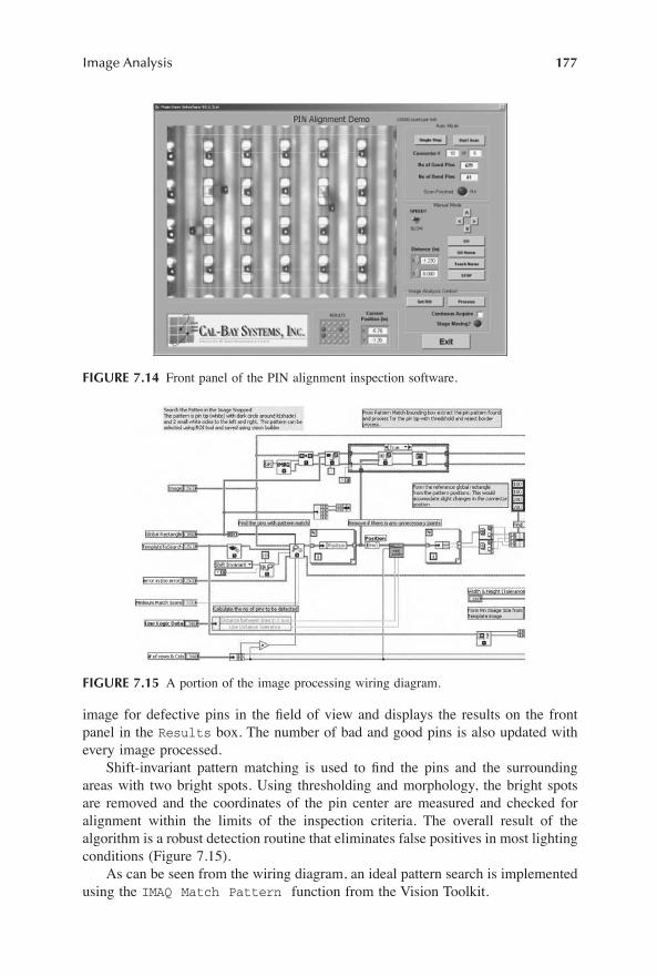
Image Analysis 177
image for defective pins in the Þeld of view and displays the results on the frontpanel in the Results box. The number of bad and good pins is also updated withevery image processed.
Shift-invariant pattern matching is used to Þnd the pins and the surroundingareas with two bright spots. Using thresholding and morphology, the bright spotsare removed and the coordinates of the pin center are measured and checked foralignment within the limits of the inspection criteria. The overall result of thealgorithm is a robust detection routine that eliminates false positives in most lightingconditions (Figure 7.15).
As can be seen from the wiring diagram, an ideal pattern search is implementedusing the IMAQ Match Pattern function from the Vision Toolkit.
FIGURE 7.14 Front panel of the PIN alignment inspection software.
FIGURE 7.15 A portion of the image processing wiring diagram.
1480_book.fm Page 177 Tuesday, June 24, 2003 11:35 AM

178 Image Acquisition Processing with LabVIEW
7.3 MATHEMATICAL MANIPULATION OF IMAGES
If you are not able to Þnd a VI within the Vision Toolkit that will perform thefunction that you need, and deÞning a custom Þlter (see Chapter 5) is not appropriate,then breaking an image into a two-dimensional array of intensity values and per-forming a custom mathematical process on them may be the only option available.
7.3.1 IMAGE TO TWO-DIMENSIONAL ARRAY
Converting an image to an array is quite simple using IMAQ ImageToArray (Figure7.16), which parses the image, and returns a two-dimensional array of 8-bit integersthat represent the intensity levels across the image (Figure 7.17). IMAQ ImageToAr-ray also has an optional rectangle input, so the user can deÞne a rectangular ROIof intensities to be returned.
7.3.2 IMAGE PORTIONS
Rather than returning a two-dimensional array of a complete image or a rectangularROI, IMAQ GetPixelValue, IMAQ GetRowCol and IMAQ GetPixelLine areuseful when you need to extract particular predeÞned portions of an image. In theexample shown in Figure 7.18, the user has selected a pixel in the middle of theimage, and IMAQ GetPixelValue has returned the intensity value of that pixel.IMAQ GetRowCol has also been used to return intensity contours of the horizontalrow and vertical column that intersect at the PUI, and IMAQ GetPixelLine returnsthe intensity values along an arbitrary line from the top left corner of the image tothe bottom right (Figure 7.19).
IMAQ SetPixelValue, IMAQ SetRowCol and IMAQ SetPixelLine acceptnew intensity value inputs, allowing you to set the intensity values of image portions(Figure 7.20). As you can see in Figure 7.21, the user can set the new intensity
FIGURE 7.16 Convert grayscale image to two-dimensional array.
1480_book.fm Page 178 Tuesday, June 24, 2003 11:35 AM

Image Analysis 179
value for the PUI. The user can also deÞne a multiplier for the selected row (thecurrent intensity values are multiplied by this number), and a divider for the selectedcolumn. Notice how the multiplied row seems noisy; this is because the calculatednew intensity values are more than 255 (the data is limited to an unsigned 8 bitinteger), therefore the new values wrap to lower levels.
FIGURE 7.17 Convert grayscale image to two-dimensional array � wiring diagram.
FIGURE 7.18 Grayscale image portions to mathematical values.
1480_book.fm Page 179 Tuesday, June 24, 2003 11:35 AM

180 Image Acquisition Processing with LabVIEW
FIGURE 7.19 Grayscale image portions to mathematical values � wiring diagram.
FIGURE 7.20 Mathematical values to grayscale image portions � wiring diagram.
FIGURE 7.21 Mathematical values to grayscale image portions.
1480_book.fm Page 180 Tuesday, June 24, 2003 11:35 AM

Image Analysis 181
7.3.3 FILLING IMAGES
You can use IMAQ FillImage to change every pixel in an image to a particularintensity value. The basic example in Figure 7.22 was achieved using the code shownin Figure 7.23. Filling an image with one intensity value is analogous to using theReplace Array Subset primitive, changing every value in a two-dimensional arrayto a particular value (Figure 7.24).
Filling images with a particular intensity value may be useful to effectivelydestroy the source image�s data, but IMAQ FillImage also has a mask input,allowing you to mask areas of the image so they are not Þlled. Consider the imageof the power meter in Figure 7.25. If a mask is created that covers the barcodelabel, the rest of the image can be easily Þlled. Once the masking has beenperformed, only the necessary image data is retained. Filling the image (Figure7.26) in this way also decreases the image�s Þle size when using a compressingimage Þle type (e.g., JPEG).
FIGURE 7.22 Fill image.
FIGURE 7.23 Fill image � wiring diagram.
1480_book.fm Page 181 Tuesday, June 24, 2003 11:35 AM

182 Image Acquisition Processing with LabVIEW
FIGURE 7.24 Fill Array.
FIGURE 7.25 Fill image with masking.
FIGURE 7.26 Fill image with masking � wiring diagram.
1480_book.fm Page 182 Tuesday, June 24, 2003 11:35 AM

Image Analysis 183
7.4 USER SOLUTION: IMAGE PROCESSING WITH MATHEMATICA LINK FOR LABVIEW
Dave RitterBetterVIEW Consulting13531 19th AvenueSouth Surrey, B.C., Canada V4A 6B3Tel (604) 535 2456/Fax (604) 501 6102e-mail: [email protected] site: http://www.bettervi.com
The IMAQ image processing tools are ideal for quickly developing a turnkeymachine vision solution. However, in the early stages of a project, it is oftenconvenient to acquire an image and experiment with it interactively. If you wouldlike to experiment with different processing techniques, or perhaps optimize thelighting placement and camera position, an interactive and immediate command-line interface offers some compelling advantages.
One powerful, command-driven request/response interface well suited to inter-active experimentation can be found in Mathematica from Wolfram Research. Math-ematica�s sophisticated symbolic capabilities and interactive �notebook� interfacemake it the tool of choice for countless scientists, researchers, and engineers world-wide, and with the help of BetterVIEW�s Mathematica Link for LabVIEW, you canintegrate Mathematica into your LabVIEW workßow. Not only does this solutionoffer you the power and immediacy of a command-line interface during the initialanalysis and design phases, it also permits you to develop turnkey, Mathematica-enabled VIs with complete access to Mathematica�s advanced symbolic, statistical,and mathematical capabilities.
Admittedly, this solution is not for everyone. However, if you are comfortablewith technical image processing terminology, and some of the underlying mathe-matical principles, introducing Mathematica and the Mathematica Link for Lab-VIEW into your workßow will permit you a much greater degree of control overthe low-level number-crunching details.
7.4.1 A TYPICAL LABVIEW/MATHEMATICA HYBRID WORKFLOW
In the initial phase, our objective is simply to acquire an image into Mathematicausing LabVIEW and National Instruments hardware. Once the image has beenacquired, we will process it interactively in the Mathematica notebook. When thisinitial experimentation phase is complete, we can determine whether to develop theÞnal application using IMAQ, or if we would prefer the lower-level control offeredby a hybrid LabVIEW/Mathematica solution.
Using Mathematica Link for LabVIEW, we begin by calling a LabVIEW-basedvideo capture VI to acquire the image, as shown in the notebook in Figure 7.27. Wehave the option of either passing the image data across the �link� as numerical data,or simply saving the image in a Þle. In this example, we have chosen to save theimage in a Þle to simplify the image data manipulations at both ends of the link.
1480_book.fm Page 183 Tuesday, June 24, 2003 11:35 AM

184 Image Acquisition Processing with LabVIEW
(The image acquisition VI is conÞgured to automatically save the acquired imagesinto the Mathematica �Images� folder.)
Once the image has been acquired, it is loaded into Mathematica for interactiveexperimentation, as shown below. While this initially may look like a lot of typingto do, it is important to note that this notebook can be saved in it entirety. All of
the processing steps can be duplicated exactly simply by specifying a new Þle nameand executing the notebook. As the notebook compiles a record of the entire sessionas you proceed, you can easily trace the path leading to the desired result. Further-more, you can accurately evaluate and compare today�s results with results fromdays, weeks, or even months past. All of the pertinent information is in the notebook,thus eliminating the need to keep accurate notes elsewhere � and much of theguesswork if others need to recreate your experiments (Figure 7.28).
It should be noted that the processing steps revealed in the Þgure take advantageof the Mathematica Digital Image Processing toolkit. However, because this toolkitis built entirely using native Mathematica functions, advanced users have the optionof developing their own sophisticated image processing tools to meet very speciÞcrequirements, or to avoid incurring the extra expense of the toolkit.
7.4.2 TAKING THE NEXT STEP
If you are involved in research, the interactive experimentation phase outlined abovemay provide all the results you are seeking. In other situations, this initial phasewill provide useful information if you are planning to process several images in asimilar fashion. Perhaps you ultimately want to develop a stand-alone image pro-cessing solution to automate the process for less sophisticated end users. At thispoint, you can turn to the IMAQ tools and develop a standard LabVIEW-basedsolution, or you can develop a hybrid Mathematica Link for LabVIEW application.
FIGURE 7.27 Mathematica notebook.
1480_book.fm Page 184 Tuesday, June 24, 2003 11:35 AM

Image Analysis 185
FIGURE 7.28 An interactive experimentation example.
1480_book.fm Page 185 Tuesday, June 24, 2003 11:35 AM

186 Image Acquisition Processing with LabVIEW
Link-based hybrids take advantage of LabVIEW�s easy-to-use GUI and Mathemat-ica�s advanced mathematical capabilities.
7.4.3 LABVIEW/MATHEMATICA HYBRID APPLICATIONS
A simple example of this hybrid approach is shown in Figure 7.29. This VI wasprepared as a demonstration of image processing using Mathematica Link for Lab-VIEW for NI Week 2002.
Note that the only National Instruments component in this system is LabVIEWitself. The image acquisition camera was an inexpensive Firewire Webcam, and theimage processing was accomplished using Mathematica and its Image Processingadd-ons. When compared with the cost of NI vision hardware and the IMAQ toolkit,this demonstrates a lower-cost option for less-critical image processing requirements.More information about Mathematica can be found at http://www.wolfram.com.Mathematica Link for LabVIEW is available from Wolfram or directly from Bet-terVIEW at http://www.bettervi.com.
FIGURE 7.29 A hybrid Mathematica-LabVIEW application.
FIGURE 7.30 Histograph example.
1480_book.fm Page 186 Tuesday, June 24, 2003 11:35 AM

Image Analysis 187
7.4.4 HISTOGRAMS AND HISTOGRAPHS
A histogram can be a very useful tool for determining the intensity distribution ofan image. The formal deÞnition of a histogram is
�a bar graph of a frequency distribution in which the widths of the bars are proportionalto the classes into which the variable has been divided and the heights of the bars areproportional to the class frequencies.
A more practical explanation is to consider a histogram as a bar chart of intensityagainst intensity occurrence, with uniform intensity bandwidths (Figure 7.30).
The Vision Toolkit has two VIs that compute the histogram of an image:IMAQ Histograph and IMAQ Histogram. IMAQ Histograph returns a clustercontaining the calculated histogram suitable for wiring directly into a front panelgraph. It also returns the histogram�s mean value and standard deviation (Figure7.31).
IMAQ Histogram returns a cluster of data that includes the same informationas IMAQ Histograph, but also contains the raw histogram as a one-dimensionalarray, the minimum and maximum values, and the histogram�s area (in pixels)(Figure 7.32 and Figure 7.33).
FIGURE 7.31 Histograph example � wiring diagram.
FIGURE 7.32 Histogram example.
1480_book.fm Page 187 Tuesday, June 24, 2003 11:35 AM

188 Image Acquisition Processing with LabVIEW
There is also the ability to deÞne an interval range over which the histogram isto be calculated. Both IMAQ Histogram and IMAQ Histograph allow the user tospecify the number of classes to sort the intensity values into, although the numberof obtained classes differs from the speciÞed value when the minimum and maximumboundaries are overshot in the interval range (Figure 7.34). The default number of
classes is 256, which is most appropriate for 8-bit images. This value gives acomplete class distribution: one class for each grayscale intensity in an 8-bit image.If the interval range minimum and maximum values are both set to zero (the default),the histogram will be calculated between 0 and 255 for 8 bit images. However, otherimage types will spread the number of classes between the lowest and highestdetected pixel intensities.
FIGURE 7.33 Histogram settings.
FIGURE 7.34 Histogram settings � wiring diagram.
1480_book.fm Page 188 Tuesday, June 24, 2003 11:35 AM

Image Analysis 189
7.5 USER SOLUTION: AUTOMATED INSTRUMENTATION FOR THE ASSESSMENT OF PERIPHERAL VASCULAR FUNCTION
Anne M. BrumÞeld and Aaron W. SchopperNational Institute of Occupational Safety and Health1095 Willowdale RoadMorgantown, WV 26505-2888Tel 304-285-6312/Fax 304-285-6265Email: [email protected]
Methods for quantifying the injurious effects of vibration are a major focus for thoseevaluating hand arm vibration syndrome (HAVS) in the workplace. The physiologicchanges in the microcirculation that occur following vibration exposure are not wellunderstood; therefore, methods for evaluating blood ßow in exposed worker popu-lations are of particular interest.
A nail press test (Figure 7.35) has been used by clinicians to assess peripheral circu-latory function. Following a 10-second press of the Þngernail, a visual determinationof the rate of blood ßow return is made, as evidenced by the return of color to theÞngernail. Of a qualitative and subjective nature, the test has been deemed mostmeaningful when used as one among several in a battery of health effect assessmenttests.1,2 New instrumentation representing an automated version of the nail press has
FIGURE 7.35 Initial user interface.
1 Olsen, N. (2002). Diagnostic aspects of vibration-induced white Þnger. Int. Arch. Occup. Environ.Health, 75: 6�13.2 Harada, N. (1987). Esthesiometry, nail compression and other function tests used in Japan for evaluatingthe hand�arm vibration syndrome. Scand. J. Work Environ. Health, 13: 330�333.
1480_book.fm Page 189 Tuesday, June 24, 2003 11:35 AM

190
Image Acquisition Processing with LabVIEW
been built utilizing a CMOS camera, and force and photoplethysmograph transducers.A LabVIEW interface, enabling simultaneous image and data acquisition, provides abasis for the standardization of the force application and duration. The raw data ispostprocessed and analyzed automatically, thereby eliminating observer subjectivity,and providing quantitative results with which worker populations can be evaluated.
7.5.1 T
HE
H
ARDWARE
The following components were incorporated into the system design (Figure 7.36):
• National Instruments AI-16XE-50 DAQ Card• National Instruments PCI-1411• National Instruments SC-2043-SG, strain gauge accessory• Miniature CMOS Camera (1/3 inch format, 510
×
492 array size)• Load cell• Photoplethysmograph transducer, power supply, amplifier (Biopac)
7.5.2 T
HE
S
OFTWARE
7.5.2.1 DAQ
An interactive front panel (Figure 7.35) provides access to a variety of VIs withina waiting state machine. Relevant subject data is entered by the operator, includingID number, finger and room temperature, handedness and finger designation, whichare incorporated into the appropriate file header or directory designation.
FIGURE 7.36
Image press prototype (rear view).
1480_C07.fm Page 190 Tuesday, June 24, 2003 4:13 PM

Image Analysis
191
The
Resting Preview
VI provides image and transducer verification, andallows focus and finger placement adjustments to be made while familiarizing thesubject with the procedure. The
Resting Data
VI collects 30 seconds of analoginput data, providing baseline measurements of the pulse volume and resting fingerforce. From these measurements, the
Resting Mean
global variable is populated,and target force values for subsequent use during the nail press are computed fromthis value. As images are not acquired here, data is gathered at a high collection rate(1024 Hz) and provides an additional resource of data for any subsequently desiredfrequency analysis measurements requiring higher resolution.
The
Nail Press
VI utilizes its front panel interface to instruct and prompt thesubject accordingly. The test consists of two sequences but starts only after theoccurrence of a hardware trigger. This trigger starts a counter on the DAQ card,which generates a square pulse wave that serves to initiate each buffer of the imageacquisition. During the initial sequence (the first 10 seconds), the interface providesan audible prompt and visual instructions to “Rest and Relax” while resting imagesand analog input data are gathered at 128 Hz. The subject is then instructed to “pressand hold” in order to reach a desired target force, calculated by adding a load cellcalibrated force to the RESTING MEAN global value. Once the target is exceeded,a countdown of 10 seconds begins, during which the subject maintains the targetforce level. The subject is then prompted to “rest and relax” for 20 additional secondsof data collection. A browser (Figure 7.37) is created which displays the imagesacquired during the press for verification of analysis results, and all images and rawdata are written to file for postprocessing and analysis. The generation of timestamped data for timing verification purposes was essential, as this VI was expandedand elaborated upon for functionality. The use of software synchronization was notproblematic at the low image acquisition rate (1 Hz); however, the use of hardwaresynchronization, which provides resolution in the order of nanoseconds, will be usedwhen higher collection rates are desired.
7.5.2.2 Postprocessing and Analysis
Characteristic force and blood volume responses during the nail press are shown inFigure 7.38. The nail press sequence may be reviewed within the
Image Analysis
VI, which cycles through the acquired images at a user-defined speed (Figure 7.39).As each image is displayed, a histogram is generated and data from this report isunbundled and saved for further analysis. Although acquired as RGB images, thehistograms are generated from their 8-bit representations. From the histogram data,selections are made for those classes demonstrating the most significant changeduring the press, and an evaluation of the pixel numbers within these bins over timegenerates a curve which, not surprisingly, resembles the curves of the force andblood volume results.
Critical to the automation of the nail press was the development of an algorithmthat could be applied in the analysis of all of the data. Such an algorithm wasdeveloped and incorporated into both the
Image Analysis
and
Data Analysis
VIs. The typical image, force and blood volume data all revealed steep slopes duringthe nail press; therefore, the data were analyzed by taking step derivatives along the
1480_C07.fm Page 191 Tuesday, June 24, 2003 4:13 PM

192
Image Acquisition Processing with LabVIEW
course of the press. Plotting the absolute values of these results reveals the areas ofmaximal change as defined by sharp peaks above baseline. The times correspondingto these peaks are calculated, and represent the times of maximal change during thenail press. The final results following the application of the step differentiationalgorithm to the image data, and the force and blood volume data respectively, areshown in Figure 7.40.
7.5.3 S
UMMARY
Using results gained from the developed instrumentation, it is possible to moreaccurately determine the times, which parallel the application of force and the returnof blood flow and color to the finger. As demonstrated, the accuracy of the result islimited by the resolution of the acquisition system; therefore increasing the imageacquisition rate above 1 Hz will certainly provide more precise determinations. Thisautomated system provides a valuable method for the evaluation of blood flow invibration-exposed worker populations.
FIGURE 7.37
Changes during a nail press.
FIGURE 7.38
Representative force and blood volume data.
1480_C07.fm Page 192 Tuesday, June 24, 2003 4:13 PM

Image Analysis 193
FIGURE 7.39 Pattern matching image analysis user interface.
FIGURE 7.40 Time extraction � load cell and photoplethysmograph data.
1480_book.fm Page 193 Tuesday, June 24, 2003 11:35 AM

194 Image Acquisition Processing with LabVIEW
7.6 INTENSITY PROFILES
Intensity proÞles are one of the most commonly used vision tools. They allow theuser to determine the pixel intensities and therefore their rates of change about aROI (Figure 7.41).
IMAQ ROIProfile uses the input image and a deÞned ROI to determine theintensity contour, which it returns in a format appropriate to wire directly to a frontpanel graph (Figure 7.42).
7.7 PARTICLE MEASUREMENTS
7.7.1 SIMPLE AUTOMATED OBJECT INSPECTION
One of the simplest machine vision VIs to begin toying with is IMAQ Count Objects.Although the name suggests that it will return a number of detected objects, it doesmuch more than that. Consider an acquired image of some pharmaceutical tablets
The simplest intensity proÞle is the point � a single value that represents the intensity of the PUI. IMAQ Light Meter (Point) is used to return this value from a deÞned x,y position.
Pixel Contour
A line intensity proÞle is a one-dimensional array of values that represent the intensity of the pixels along the line, as drawn from the Þrst to the last point. This example was achieved using IMAQ Light Meter (Line).
Line Contour
A closed ROI returns a one-dimensional array whose values trace around the ROI from the initial deÞned point in a clockwise direction. As shown in the example, the intensity proÞle midpoint is approximately 125 pixels of travel from the Þrst ROI point, therefore the Þrst 125 points of the proÞle correspond to the upper and right sides of the ROI. The values after 125 represent the lower and left sides of the ROI.
Closed ROI ContourFIGURE 7.41
1480_book.fm Page 194 Tuesday, June 24, 2003 11:35 AM

Image Analysis 195
(Figure 7.43). By using IMAQ Count Objects you can obviously count the numberof tablets, but it also returns quite a lot of information about each of them, includingeach tablet�s position with respect to the top left corner of the image, its boundingbox, and how many holes (if any) were detected within it.
FIGURE 7.42 Closed ROI contour � wiring diagram.
FIGURE 7.43 White tablets with a black background.
FIGURE 7.44 Count objects.
1480_book.fm Page 195 Tuesday, June 24, 2003 11:35 AM

196 Image Acquisition Processing with LabVIEW
This technique is very easily achieved by deÞning the settings of the searchroutine (Table 7.4). Although the search rectangle input suggests that by leavingit unwired it will search the whole image, this is not the case � you will need toset some sort of search rectangle either manually or programmatically for theIMAQ Count Objects routine to work (Figure 7.45).
As you can see from the example (Figure 7.44), 11 objects were detected(numerated from 0 to 10), including the irregularly positioned tablet on the rightside of the image, and the partially obscured tablet on the left. The tablet on its end
TABLE 7.4“Count Objects Settings” Cluster Elements
Setting DescriptionObjects You can select whether the search routine should look for dark or light
objects (with respect to the background).Threshold This is the grayscale intensity that is used as a threshold level.Ignore Objects touching Image Borders
If a detected image intersects the deÞned search rectangle, it is not included as a counted image.
Fill Holes within Objects If a detected object contains holes (regions within its bounds that are on the opposite side of the threshold descriptor) then they are Þlled, and the object is considered as a single entity.
Minimum Objects Size & Min Size
If an object is detected that is smaller than this size, it is ignored. This can be very useful when you do not have a perfectly populated image (e.g., excessive noise, dust or other contaminants are creating false �objects�).
Maximum Object Size & Max Size
As you might expect, any detected objects larger than the Max Size are ignored.
Show Search Area If set to true, a green box is overlaid on the image to show the search area.
Show Bounding Box As demonstrated in the example above, the bounding box of detected objects is shown as an overlaid red box with an integer corresponding to the object�s number (as referenced by the �objects� output array).
Show Object Center Also as demonstrated above, the center of the Bounding Box is drawn as a small dot overlaid on the image.
FIGURE 7.45 Count objects � wiring diagram.
1480_book.fm Page 196 Tuesday, June 24, 2003 11:35 AM

Image Analysis 197
is detected as an object, because this routine is simply looking for objects that standout from the background � not those that conform to particular predeÞned criteria,such as shape, color or size.
If the search rectangle is limited, IMAQ Count Objects will include objectspartially bound by the search rectangle, and return their positions, bounding boxes,and number holes with respect to the image within the search rectangle (Figure 7.46).
Setting the options to ignore objects that touch the search rectangle will consideronly objects that are wholly within the rectangle (Figure 7.47).
7.7.2 MANUAL SPATIAL MEASUREMENTS
Measuring the distance between two points can be very easily accomplished byusing Pythagoras� theorem (Figure 7.48). If we can determine the spatial coordi-nates of the two points between which we want to measure, then calculating the
FIGURE 7.46 Count objects � limited search rectangle.
FIGURE 7.47 Count objects � objects touching search rectangle.
1480_book.fm Page 197 Tuesday, June 24, 2003 11:35 AM

198 Image Acquisition Processing with LabVIEW
FIGURE 7.48 Pythagoras� Theorem.
FIGURE 7.49 Measure between points.
FIGURE 7.50 Measure between points � wiring diagram.
Distance x y x y x yA A B B( ) ( )[ ] = ( ) + ( ), D D2 2 Dxy
Axy
Bxy
dx
dy
X
Y
1480_book.fm Page 198 Tuesday, June 24, 2003 11:35 AM

Image Analysis 199
distance between them is trivial. For example, if a user draws a line ROI betweentwo points, the pixel distance between them can be easily determined (Figure 7.49and Figure 7.50).
While this is simple when we know the spatial positions of the two points, itbecomes more difÞcult when their coordinates must be determined programmatically.
7.7.3 FINDING EDGES PROGRAMMATICALLY
An edge in an image is generally deÞned as a feature interface with high contrast;if an image�s intensity changes dramatically within a small spatial range, then it canbe considered as an edge. The IMAQ Edge Tool can be used to detect and classifyedges in an image by inspecting the pixel intensity values along a trace applied tothe image. The example in Figure 7.51 obtains the pixel coordinates of points alonga line ROI drawn by the user, and uses them to search for edges.
The pixel coordinates are obtained using IMAQ ROIProfile, and are wired intoIMAQ Edge Tool. IMAQ Edge Tool outputs the number of edges detected, theircoordinates and an array of clusters detailing comprehensive information regardingeach of the edges (Figure 7.52).
IMAQ Edge Tool is conÞgured by deÞning the edge parameters to use duringthe search. Contrast speciÞes the threshold for the edge�s intensity differencebetween features � edges with a contrast less than this threshold are not treated asedges, and are subsequently ignored. The contrast is calculated as the difference
FIGURE 7.51 Finding edges and their parameters � wiring diagram.
FIGURE 7.52 Finding edges and their parameters.
1480_book.fm Page 199 Tuesday, June 24, 2003 11:35 AM

200 Image Acquisition Processing with LabVIEW
between the average pixel intensity before the edge and the average pixel intensityafter the edge over the Þlter width (Figure 7.53), which is the maximum andminimum number of pixels over which you deÞne an edge can occur. A small Þlterwidth ensures that the change in contrast occurs rapidly, whereas a larger Þlter widthallows for a more gradual change.
Consider a pixel position a. The contrast is determined by considering the pixelsalong the line of interest, both before and after a, that exist within the Þlter width:
The edge information array output of IMAQ Edge Tool contains an array ofclusters, each describing respective detected edges. The two elements of the clusterdescribe the position, which deÞnes the pixel coordinate location of the detectededge. This output is not the (x,y) position of the edge, nor does it represent the pixelnumber along the ROI where the edge is detected. When IMAQ Edge Tool executes,it searches the intensities that correspond to the pixel locations deÞned in the pixelcoordinates input. This input in not necessarily linear, nor continuous. It is possibleto deÞne the pixel coordinates, so that IMAQ Edge Tool inspects pixels that are farfrom each other. For example, the array shown in Figure 7.54 is an entirely validpixel coordinates input.
This example shows a spatial discontinuity between the 3rd and 4th elements.IMAQ Edge Tool does not interpolate between these coordinates, instead it considersthem as continuous, and applies the edge detection across them.
The edge information array output also contains the contrast of the detectededge, and the polarity. A polarity of 1 indicates a rising edge (the intensities arechanging from dark to light), whereas a polarity of �1 indicates a falling edge (lightto dark).The Þnal output cluster element is called score, and is unused.
FIGURE 7.53 Edge parameters.
Filter Width
Steepness
Con
trast
Distance Along Pixel Coordinate Path
Pix
el In
tens
ity
Contrast I x I xx a
x a
x a
x a
fw
fw
=È
Î
ÍÍÍ
ù
û
úúú∏
È
Î
ÍÍÍ
ù
û
úúú= -( )
=
=
= +( )Â Â( ) ( )
2
2
1480_book.fm Page 200 Tuesday, June 24, 2003 11:35 AM
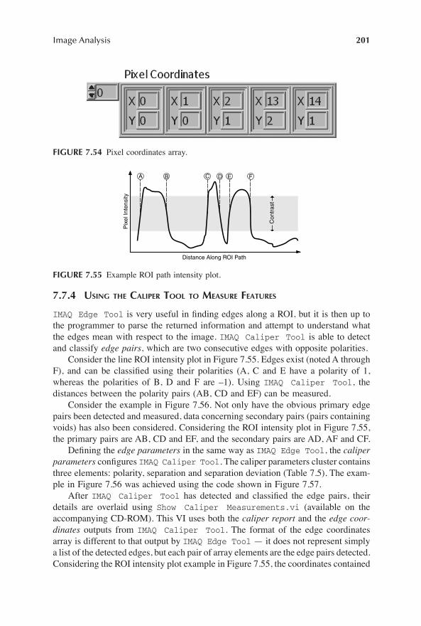
Image Analysis 201
7.7.4 USING THE CALIPER TOOL TO MEASURE FEATURES
IMAQ Edge Tool is very useful in Þnding edges along a ROI, but it is then up tothe programmer to parse the returned information and attempt to understand whatthe edges mean with respect to the image. IMAQ Caliper Tool is able to detectand classify edge pairs, which are two consecutive edges with opposite polarities.
Consider the line ROI intensity plot in Figure 7.55. Edges exist (noted A throughF), and can be classiÞed using their polarities (A, C and E have a polarity of 1,whereas the polarities of B, D and F are �1). Using IMAQ Caliper Tool, thedistances between the polarity pairs (AB, CD and EF) can be measured.
Consider the example in Figure 7.56. Not only have the obvious primary edgepairs been detected and measured, data concerning secondary pairs (pairs containingvoids) has also been considered. Considering the ROI intensity plot in Figure 7.55,the primary pairs are AB, CD and EF, and the secondary pairs are AD, AF and CF.
DeÞning the edge parameters in the same way as IMAQ Edge Tool, the caliperparameters conÞgures IMAQ Caliper Tool. The caliper parameters cluster containsthree elements: polarity, separation and separation deviation (Table 7.5). The exam-ple in Figure 7.56 was achieved using the code shown in Figure 7.57.
After IMAQ Caliper Tool has detected and classiÞed the edge pairs, theirdetails are overlaid using Show Caliper Measurements.vi (available on theaccompanying CD-ROM). This VI uses both the caliper report and the edge coor-dinates outputs from IMAQ Caliper Tool. The format of the edge coordinatesarray is different to that output by IMAQ Edge Tool � it does not represent simplya list of the detected edges, but each pair of array elements are the edge pairs detected.Considering the ROI intensity plot example in Figure 7.55, the coordinates contained
FIGURE 7.54 Pixel coordinates array.
FIGURE 7.55 Example ROI path intensity plot.C
ontr
ast
Distance Along ROI Path
Pix
el In
tens
ity
A B C D E F
1480_book.fm Page 201 Tuesday, June 24, 2003 11:35 AM

202 Image Acquisition Processing with LabVIEW
FIGURE 7.56 Using the caliper.
TABLE 7.5“Caliper Parameters” Cluster Elements
Element DescriptionPolarity This controls what are to be considered the leading and trailing edges
during the search. There are Þve possible polarity settings:None: All edges are considered as leading and trailing edges.Dark-Light: Leading=Dark, Trailing=LightLight-Dark: Leading=Light, Trailing=DarkDark-Dark: Both Leading and Trailing=DarkLight-Light: Both Leading and Trailing=Light
Separation SpeciÞes the expected spatial difference between the edge pairs. Only edge pairs around this value (within the tolerance deÞned by the separation deviation) are considered. If separation is set to 0, all edge pairs detected are considered.
Separation deviation DeÞnes the tolerance value for the separation between the edges.
FIGURE 7.57 Using the caliper � wiring diagram.
1480_book.fm Page 202 Tuesday, June 24, 2003 11:35 AM

Image Analysis 203
in the array would represent the edge pairs in the following order: AB, AD, AF, CD,CF, EF, therefore the array element values would be as shown in Figure 7.58.
7.7.5 RAKING AN IMAGE FOR FEATURES
7.7.5.1 Parallel Raking
Just as a garden rake has several tines that create parallel lines in the dirt, an imagerake is a series of parallel line ROIs, deÞned by their start and end points, and therelative distance between each line (Figure 7.59 and Figure 7.60).
Raking an image can be very useful when trying to Þnd a feature in an image.Consider the example in Figure 7.59. If the part were shifted vertically, a singlehorizontal line ROI may fail to locate the hole in the pin, whereas using a rake candetermine where the hole is, and its dimensions. IMAQ Rake is conÞgured using theinputs in Table 7.6. The IMAQ Rake function returns an array of clusters, whereeach array element corresponds to a rake line. The clusters contain an array ofclusters, each specifying the edge coordinates found along the rake line.
FIGURE 7.58 ROI intensity plot edge coordinates.
FIGURE 7.59 Parallel raking example.
FIGURE 7.60 Parallel raking example � wiring diagram.
1480_book.fm Page 203 Tuesday, June 24, 2003 11:35 AM

204 Image Acquisition Processing with LabVIEW
7.7.5.2 Concentric Raking
Concentric circles share a common origin (as an aside, concentricity is the oppositeto eccentricity), so concentric raking occurs when the rake lines follow circles witha common origin. Concentric raking is particularly useful when inspecting parts thathave features intersecting with circular features (Figure 7.61).
In the example (Figure 7.61), IMAQ Concentric Rake has found edges alongconcentric circular paths as deÞned by the annulus ROI. The positions of the detectededges are the output, and can be used to reconstruct a line model of the image, ordetect where sections of the cross beams are missing. IMAQ Concentric Rake useis similar to IMAQ Rake, except the scan direction is deÞned as either clockwise orcounterclockwise (default) (Figure 7.62).
TABLE 7.6“IMAQ Rake” Inputs
Input DescriptionEdge Parameters This input deÞnes what should be considered as an edge. See Section 7.7.3,
Finding Edges Programmatically, for more details.Scan Direction You can deÞne the direction that edges are searched for along the lines. The
following settings are permitted:Left to right (default)Right to leftTop to bottomBottom to top
Step Size DeÞnes the distance, in pixels, between the parallel lines inside the rectangular region.
FIGURE 7.61 Concentric raking example.
1480_book.fm Page 204 Tuesday, June 24, 2003 11:35 AM

Image Analysis 205
7.7.5.3 Spoke Raking
When you are searching for circular features in an image, spoke raking can be avery powerful tool. Similar to parallel raking, spoke raking performs edge detectionalong rake lines, although they are not parallel. When spoke raking, the rake linesare portions of radial lines (Figure 7.63).
An arc or circular object can be mapped using the edge coordinates (Figure7.64) output of IMAQ Spoke. IMAQ Spoke is conÞgured using the inputs shown inTable 7.7.
FIGURE 7.62 Concentric raking example � wiring diagram.
FIGURE 7.63 Spoke example.
1480_book.fm Page 205 Tuesday, June 24, 2003 11:35 AM

206 Image Acquisition Processing with LabVIEW
TABLE 7.7
Input DescriptionEdge Parameters This input deÞnes what should be considered as an edge. See section 7.7.3,
Finding Edges Programmatically, for more details.Scan Direction You can deÞne the direction that edges are searched for along the lines. The
following settings are permitted:Outside to inside (default)Inside to outside
Step Size DeÞnes the distance, in pixels, between the radial lines inside the region.
FIGURE 7.64 Spoke example � wiring diagram.
1480_book.fm Page 206 Tuesday, June 24, 2003 11:35 AM

Image Analysis 207
7.8 USER SOLUTION: SISSON-AMMONS VIDEO ANALYSIS (SAVA) OF CBFS
Bruce A. Ammons, Ph.D.President � Ammons Engineering8114 Flintlock Rd., Mt. Morris, MI 48458Tel (810) 687-4288/Fax (810) 687-6202e-mail: [email protected] site: http://www.ammonsengineering.comJoseph H. Sisson, M.D.Professor of MedicineUniversity of Nebraska Medical Center
The University of Nebraska Medical Center needed a fast, efÞcient, and easy touse system to accurately measure the beat frequency of ciliated cells. AmmonsEngineering designed the Sisson-Ammons Video Analysis (SAVA) system usingLabVIEW and IMAQ Vision to record video directly into the computer and analyzethe ciliary beat frequency (CBF), greatly reducing the time required to run eachexperiment.
7.8.1 INTRODUCTION
In the lungs, cells that line the trachea and bronchi (which are the conducting tubesof the lungs) have microscopic, hair-like appendages called cilia. Cilia beat in asynchronized pattern to propel mucus and inhaled particles out of the lungs. Dr.Joseph H. Sisson, Professor of Medicine at the University of Nebraska MedicalCenter, needed to upgrade a system developed using LabVIEW 2.1 in 1991 to afaster system using current technology. The system measures the CBF of airwaytissues to determine the effect of various reagents, such as those found in medicinesor in cigarette smoke. By adding the reagents to the cell samples and recording thechange in the CBF over time, the effects of the medicines or toxins can be quantiÞed.A typical experiment may have four or Þve different conditions with three or foursamples for each condition. The system needed to be capable of recording each ofthe samples in half-hour intervals.
7.8.2 MEASUREMENT OF CILIA BEAT FREQUENCY (CBF)
To measure the cilia beat frequency; ciliated cells are grown on tissue culturedishes and incubated for several days until the cells are stable. This gives thecells time to group together and attach to the surface of the dishes. Before addingany reagents, a baseline CBF measurement is made for each sample. After addingreagents to the samples, brief measurements (approximately 5 seconds in dura-tion) are recorded periodically for up to a 24-hour period. To measure the beatfrequency, a sample is placed under an inverted phase contrast microscope anda group of motile cells is located, as shown in Figure 7.65. Video is acquiredusing a high-speed digital video camera mounted on the microscope that is capable
1480_book.fm Page 207 Tuesday, June 24, 2003 11:35 AM

208 Image Acquisition Processing with LabVIEW
of capturing digital images at up to 85 fps. At a single point, the light intensity alternatesbetween light and dark each time cilia passes beneath the point. This variation in theintensity is used to measure the CBF. The operator selects a region of interest on thevideo image, which can be a point, a rectangle, or a line.
For each image in the video, the intensity of the pixels within the region isaveraged and converted to a waveform representing the average intensity over time.This waveform is analyzed using standard LabVIEW tools to extract the dominantfrequency and its amplitude.
The new system divides the CBF measurement process into two major phases.The Þrst is the recording of the video, and the second phase consists of two alternativeapproaches to measuring the frequencies. Single point analysis allows the operatorto choose the points of interest, and whole image analysis uses all of the points inthe image.
7.8.3 VIDEO RECORDING
During the video recording phase, a live digitized video image is continuouslydisplayed on the screen. The operator can adjust the frame rate, gain, and the numberof images to store. From these settings, the maximum analysis frequency, spectrumfrequency resolution, and video length in seconds are calculated and displayed. Atimer displays the amount of time elapsed since the start of the experiment.
The video is acquired directly into the computer�s memory using a circular bufferthat contains a video history of the last few seconds. The size of the buffer is slightlylarger than the number of images that will be recorded to disk. The video historyenables the operator to quickly select various points on the video and instantlymeasure the CBF at each point. Once the operator has located an area in the samplewith an adequate quantity of cells, they store the video to disk. The sample beinganalyzed is selected from the master list of samples, and the image sequence isstored along with the sample name, elapsed time and comments.
It is also possible to conÞgure the system to record video at regular intervalswithout any operator interaction. The operator can leave one sample of interest onthe microscope for recording over time. This way, the same cells are recorded atexact time intervals.
FIGURE 7.65 Locating cells using a microscope.
1480_book.fm Page 208 Tuesday, June 24, 2003 11:35 AM

Image Analysis 209
7.8.4 SINGLE POINT ANALYSIS
After recording the samples, the video is analyzed to determine the beat frequencies(Figure 7.66). Analysis of recorded samples can be done during the longer intervalsbetween recordings or after the experiment has been completed. The operator canselect any previously recorded sample from a list, which includes a summary ofanalysis results for each sample. The recorded video is displayed in a repeating loop,along with information about the sample name, date, time, elapsed time, and com-ments as shown below. The video can be paused, single stepped forward or backward,and any image can be exported in a variety of formats for inclusion in reports.
The same analysis tools available during the recording phase are available duringthe analysis phase, with a few extra features. The operator can store the results formultiple regions of interest, for which the mean and standard error are calculated.The results are automatically exported for graphing and inclusion in reports.
7.8.5 WHOLE IMAGE ANALYSIS
To signiÞcantly extend the capabilities of the system, a method to rapidly analyzelarge quantities of data was desired, and whole image analysis was the result. Theimage is divided into 4 ¥ 4 pixel blocks, and each block is analyzed using the sameroutines as the single point analysis. The result of the analysis is displayed in twointensity graphs, one for frequency and one for amplitude, as shown in Figure 7.67.The operator can eliminate values outside the valid range. An intensity graph and ahistograph of the remaining points are displayed, along with a statistical summaryof the data.
FIGURE 7.66 Single point analysis.
1480_book.fm Page 209 Tuesday, June 24, 2003 11:35 AM
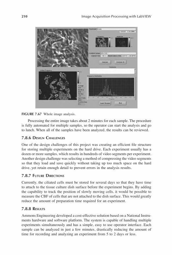
210 Image Acquisition Processing with LabVIEW
Processing the entire image takes about 2 minutes for each sample. The procedureis fully automated for multiple samples, so the operator can start the analysis and goto lunch. When all of the samples have been analyzed, the results can be reviewed.
7.8.6 DESIGN CHALLENGES
One of the design challenges of this project was creating an efÞcient Þle structurefor storing multiple experiments on the hard drive. Each experiment usually has adozen or more samples, which results in hundreds of video segments per experiment.Another design challenge was selecting a method of compressing the video segmentsso that they load and save quickly without taking up too much space on the harddrive, yet retain enough detail to prevent errors in the analysis results.
7.8.7 FUTURE DIRECTIONS
Currently, the ciliated cells must be stored for several days so that they have timeto attach to the tissue culture dish surface before the experiment begins. By addingthe capability to track the position of slowly moving cells, it would be possible tomeasure the CBF of cells that are not attached to the dish surface. This would greatlyreduce the amount of preparation time required for an experiment.
7.8.8 RESULTS
Ammons Engineering developed a cost-effective solution based on a National Instru-ments hardware and software platform. The system is capable of handling multipleexperiments simultaneously and has a simple, easy to use operator interface. Eachsample can be analyzed in just a few minutes, drastically reducing the amount oftime for recording and analyzing an experiment from 5 to 2 days or less.
FIGURE 7.67 Whole image analysis.
1480_book.fm Page 210 Tuesday, June 24, 2003 11:35 AM
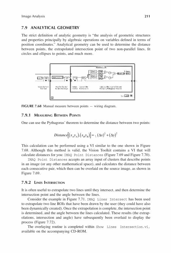
Image Analysis 211
7.9 ANALYTICAL GEOMETRY
The strict deÞnition of analytic geometry is �the analysis of geometric structuresand properties principally by algebraic operations on variables deÞned in terms ofposition coordinates.� Analytical geometry can be used to determine the distancebetween points, the extrapolated intersection point of two non-parallel lines, Þtcircles and ellipses to points, and much more.
7.9.1 MEASURING BETWEEN POINTS
One can use the Pythagoras� theorem to determine the distance between two points:
This calculation can be performed using a VI similar to the one shown in Figure7.68. Although this method is valid, the Vision Toolkit contains a VI that willcalculate distances for you: IMAQ Point Distances (Figure 7.69 and Figure 7.70).
IMAQ Point Distances accepts an array input of clusters that describe pointsin an image (or any other mathematical space), and calculates the distance betweeneach consecutive pair, which then can be overlaid on the source image, as shown inFigure 7.69.
7.9.2 LINES INTERSECTION
It is often useful to extrapolate two lines until they intersect, and then determine theintersection point and the angle between the lines.
Consider the example in Figure 7.71. IMAQ Lines Intersect has been usedto extrapolate two line ROIs that have been drawn by the user (they could have alsobeen dynamically created). Once the extrapolation is complete, the intersection pointis determined, and the angle between the lines calculated. These results (the extrap-olations, intersection and angle) have subsequently been overlaid to display theprocess (Figure 7.72).
The overlaying routine is completed within Show Lines Intersection.vi,available on the accompanying CD-ROM.
FIGURE 7.68 Manual measure between points � wiring diagram.
Distance x y x y x yA A B B( ) ( )[ ] = ( ) + ( ), D D2 2
1480_book.fm Page 211 Tuesday, June 24, 2003 11:35 AM

212 Image Acquisition Processing with LabVIEW
FIGURE 7.69 Point distances example.
FIGURE 7.70 Point distances example � wiring diagram.
FIGURE 7.71 Lines intersection example.
1480_book.fm Page 212 Tuesday, June 24, 2003 11:35 AM

Image Analysis 213
7.9.3 LINE FITTING
Fitting is a useful mathematical technique when used to discover trends in sampledata sets, and can be just as valuable when examining images. Parts under inspectionoften contain regular repeating structures, and line Þtting can be used as a qualitycontrol measure to ensure that parts are consistent. Consider Figure 7.73: A seriesof Australian ßags has been printed on a sheet, although one of the ßags has beenprinted with an incorrect alignment.
Using IMAQ Count Objects and IMAQ Fit Line, it is obvious that the thirdßag from the left is not in the correct position. The Federation star (the seven-pointedstar in the bottom left quadrant of the ßag) has been detected, and their centersdetermined. This data has been then passed to IMAQ Fit Line, which determinedthe line of best Þt. Features that are outside of a user-deÞned range of distancesfrom the Þtted line can then be regarded as inappropriate, and the part is failed(Figure 7.74).
IMAQ Fit Line does not perform a line of best Þt in the true mathematicalsense, as it can disregard some points that you include in the set to be considered.You are able to deÞne a pixel radius that deÞnes a corridor either side of the lineof best Þt, where only points within the corridor are considered. IMAQ Fit LineÞnds the line of best Þt by Þrst considering a subset of points that has beendeÞned, and subsequently calculating the mean square distance (MSD) of thisline (Figure 7.75).
FIGURE 7.72 Lines intersection example � wiring diagram.
FIGURE 7.73 Fit line example.
1480_book.fm Page 213 Tuesday, June 24, 2003 11:35 AM

214 Image Acquisition Processing with LabVIEW
The mean square distance is calculated using the following equation:
Once the MSD has been calculated, a new line of best Þt is determined using adifferent set of points, and its MSD is also calculated. This process is repeated untilall of the points in the input dataset have been considered (except those discardedfor lying outside of the pixel radius range), and the set with the lowest MSD isreturned as the line of best Þt.
The MSD approach of line Þtting was selected to minimize the impact of outlyingpoints. Consider the parallel rake application shown in Figure 7.76. If the applicationrequirement is to Þt a line to the edge of the spanner head blade, the four extremeright detected edge coordinates are erroneous, although they are perfectly validdetected edges, they do not form part of the feature that we are looking for, and areignored if the IMAQ Fit Line parameters are set appropriately.
7.9.4 CIRCLE AND ELLIPSE FITTING
If you are searching an image for a regular feature, it is often much faster to use arake and reconstruct shapes from the detected edges rather than using a patternmatch template. If you want either a circle or ellipse, the IMAQ Fit Circle andIMAQ Fit Ellipse analytical geometric tools can be helpful. IMAQ Fit Circlerequires a minimum of three points to function, although extra valid points willincrease its accuracy.
FIGURE 7.74 Fit line example � wiring diagram.
FIGURE 7.75 Line of best Þt determination.
Points not Consideredin this Set
d 0
d 1 d 2
d 3 d...
d n
Points Consideredin this Set
Line of Best Fit
MSD
d
n
a
a
n
= =
-
 2
0
1
1480_book.fm Page 214 Tuesday, June 24, 2003 11:35 AM
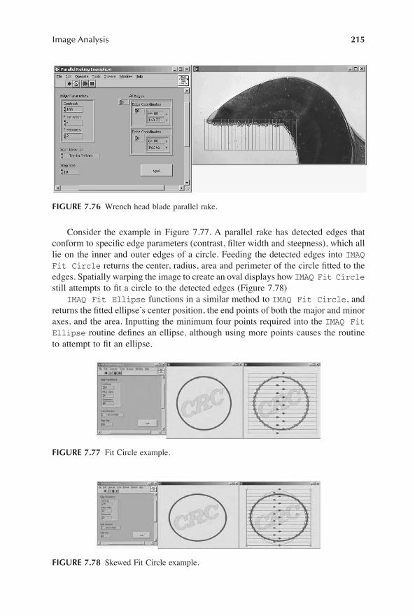
Image Analysis 215
Consider the example in Figure 7.77. A parallel rake has detected edges thatconform to speciÞc edge parameters (contrast, Þlter width and steepness), which alllie on the inner and outer edges of a circle. Feeding the detected edges into IMAQFit Circle returns the center, radius, area and perimeter of the circle Þtted to theedges. Spatially warping the image to create an oval displays how IMAQ Fit Circlestill attempts to Þt a circle to the detected edges (Figure 7.78)
IMAQ Fit Ellipse functions in a similar method to IMAQ Fit Circle, andreturns the Þtted ellipse�s center position, the end points of both the major and minoraxes, and the area. Inputting the minimum four points required into the IMAQ FitEllipse routine deÞnes an ellipse, although using more points causes the routineto attempt to Þt an ellipse.
FIGURE 7.76 Wrench head blade parallel rake.
FIGURE 7.77 Fit Circle example.
FIGURE 7.78 Skewed Fit Circle example.
1480_book.fm Page 215 Tuesday, June 24, 2003 11:35 AM

1480_book.fm Page 216 Tuesday, June 24, 2003 11:35 AM

217
8
Machine Vision
A generally accepted deÞnition of machine vision is �
�the analysis of images toextract data for controlling a process or activity.�
Machine vision is a subdisciplineof artiÞcial intelligence that uses video cameras or scanners to obtain informationabout a given environment, and to extract data from digital images about objects inthe image. Machine vision takes an image in and outputs some level of descriptionabout the objects in it (i.e., size, position, correlation, etc.). Although applicationsfor machine vision vary, there are generally only a few main categories:
� Quality assurance� Sorting� Material handling� Robot guidance� Calibration
Quality assurance
represents probably the largest number of machine visionapplications in use today. All that quality assurance machine vision systems do isinspect an image and decide whether the part should pass or fail, based on apredetermined set of rules. Although humans can be excellent quality assuranceinspectors, vision systems are appropriate when images need to be inspected athigh speed (often production lines require part inspection rates up to many complexparts per second), and for monotonous work. Vision systems do not become bored,or lack concentration; therefore, quality assurance can be much more highlycontrolled. Conversely, human inspectors can think and possibly expand or changethe pass/fail rules � this can be both advantageous and disadvantageous. If thehuman Þnds a ßaw in the product that is not part of the pass/fail criteria, then itcan be added. On the contrary, humans can interpret rules incorrectly, often leadingto quality assurance issues.
As its name suggests,
sorting
is the categorization of parts. Vision systems candetect part types based on predeÞned criteria and sort the parts accordingly. Thisdetection can also be an extension of quality assurance, where pass and fail partsare segregated, and the production process continues without human interaction.Sorting application examples include the sizing of apples in a packing plant, theremoval and remelting of excessively eccentric extruded copper tubes and the scrap-ping of Þber Bragg gratings that do not Þt a bandwidth template.
Materials handling
in hazardous environments can be simpliÞed and automatedusing machine vision. Often, materials need to be handled quickly, and in areas thatdo not conform to desirable working conditions for humans. When considering thestorage of products, warehouses populated by humans need to be well lit, and oftenuse climate control to keep workers comfortable, which could be inappropriate forthe product. Depending on the system used, machine vision systems can require
1480_book.fm Page 217 Tuesday, June 24, 2003 11:35 AM

218
Image Acquisition Processing with LabVIEW
minimal lighting or climate control to perform similar functions. Also, environmentsthat are extremely dangerous for humans such as bomb disposal, toxic waste han-dling, high radiation and high temperature environments can be managed usingmachine vision process control.
Robot guidance
often uses a close coupling of machine vision and robot controlin industries such as arc welding for car construction, spray-painting and machinetool loading and unloading. Robot guidance routines can also encapsulate learningfunctions based on images acquired using machine vision.
Calibration
of parts and assemblies can be automated using machine vision.Mechanical systems can be controlled, and their response monitored by a camera.A machine vision system can then analyze the part�s response to the mechanicalstimulus, and adjust the part to perform within a speciÞed range. Companies thatmanufacture calculators, thermostats and keyboards often use machine vision sys-tems to perform calibration.
National Instrument�s Vision Toolkit implementation of machine vision comprisesa varied tool palette, including functions that count and measure objects, distances andintensities; perform pattern matching; and read physical instrument displays.
Further information regarding machine vision theory can be found in the freeonline course
Introduction to Machine Vision
offered by Automated Vision Systems(http://www.autovis.com/courslst.html).
8.1 OPTICAL CHARACTER RECOGNITION
Optical character recognition (OCR) is the process of extracting textual data froman image, and is often used in the industrial world. From resolving the letters andnumbers on a license plate of a moving car to scanning a document and saving thetext to a Þle, OCR has become a widely accepted concept.
The IMAQ Vision OCR software is a toolkit purchased separately from theVision Toolkit, and adds several very powerful character recognition routines thatare able to quickly resolve text in a variety of ambient lighting conditions, fonts andprinting qualities.
Although the toolkit is particularly suited to reading alphanumeric charactersthat have been produced using conventional typesetting and printing, it is alsoable to read common fonts used in automotive, electronics and pharmaceuticalÞelds.
8.1.1 R
ECOGNITION
C
ONFIGURATION
To perform a simple OCR, start by calling
IMAQ OCR Recognition Config
toset the recognition parameters (there are quite a lot of them, as shown in Table 8.1).
8.1.2 C
ORRECTION
C
ONFIGURATION
After you have deÞned the recognition parameters, you can also invoke a correctionroutine called
IMAQ OCR Correction Config
. Using this VI will attempt to correctcommon textual errors based on whether you want to give preference to a particularcharacter type.
1480_book.fm Page 218 Tuesday, June 24, 2003 11:35 AM

Machine Vision
219
TABLE 8.1“IMAQ OCR Recognition Config” Parameters
Input Description
Maximum point size The OCR routine will only recognize text with a point size of this value or less (this value should be set to a value slightly above your expected point size).
Language The OCR routine can recognize characters in English, French and Spanish.
Character set If you know that the text you are trying to return has only uppercase letters, then you can instruct the OCR routine not to try and Þnd other characters (lowercase letters, numbers, punctuation, etc). Limiting the character set will not only increase the speed of the OCR routine dramatically, but also inhibit common errors (for example, mistaking
I
for
l
).Character type This input instructs the OCR routine to whether
the expected text is normal, italic or a mixture of both (note: type checking is performed on a word-level, so mixing normal and italic characters within a word may cause the OCR routine to fail).
Recognition mode There are four recognition modes:High Speed (Very fast, only good for low noise images with well spaced and deÞned characters).
Nominal (Down-samples images to 200 dpi before scanning to improve speed � nominal and balanced are identical when source images that are already 200 dpi or less).
Balanced (Good for a wide range of typeface variations and character qualities).
Unoptimized (Disables all recognition optimizations).
Auto correction When enabled, auto correction will cause the OCR routine to attempt to Þnd the closest match to characters that it does not recognize at all. If disabled, unrecognized characters are ignored.
Output delimiter This setting is only useful if you want to change the character that will appear between detected words. The available settings are None (disables the delimiter), Space (default), Tab, Comma and Full Stop (�Dot�).
1480_book.fm Page 219 Tuesday, June 24, 2003 11:35 AM

220
Image Acquisition Processing with LabVIEW
Several letters and numbers in the OCR�s character library look similar:
Using these example characters, you can see how simple text can be incorrectlyparsed:
Using
IMAQ
OCR
Correction
Config,
you can set the way ambiguouslydetected characters are interpreted. The VI has the inputs shown in Table 8.2.
8.1.3 OCR P
ROCESSING
Once you have set both the OCR recognition and correction parameters, all thatremains to do is to perform the OCR search. There are two OCR searchVIs availablein the Vision Toolkit:
IMAQ Basic OCR
and
IMAQ Complex OCR
. The only difference
Character Similar Characters
The letter
I 1 l i ! | / \ [ ] '
The letter
S 5 $
The letter
O
0 Ø
W
o
Printed String Possible OCR Results
ISO 9001 ISO 9001 1SO 900I !SO 900[
I$Ø 9WW| [50 9OO] \$Ø 9
WW
/
|S0 900| iSo 9oo! ...
TABLE 8.2“IMAQ OCR Correction Config” Inputs
Input Description
Character preference This input depends on whether you want the OCR routines to favor alphabetic or numeric characters, or neither. For example, setting the character preference to
alphabetic
will prevent errors such as ISO
Þ
1S0
.Method The method input is similar to the recognition mode input for
IMAQ OCR Recognition
ConÞg. Using this input, you are able to place more emphasis on whether the correction is faster or more accurate (default).
Aggressiveness Aggressiveness deÞnes to what extent the OCR search will attempt to parse a character that is ambiguous. When the OCR search detects a character that it is not sure about, it will compare it to a list of characters to Þnd a possible match, and setting the aggressiveness changes the list of characters to be searched:
Conservative List:
1I l | ! ] [ 0 O
Aggressive List:
1
I
l
|
! ]
[
0
O
2 Z 5 S 8 B
As you might expect, using the aggressive list will slow down OCR searching of ambiguous text.
1480_book.fm Page 220 Tuesday, June 24, 2003 11:35 AM

Machine Vision
221
between them is that
IMAQ Complex OCR
will output a report on each of the detectedcharacters � the actual OCR search and recognition routines are identical.
When performing the OCR, you can deÞne a few more parameters to make thesearch easier and faster. Both
IMAQ Basic OCR
and
IMAQ Complex OCR
have theinputs shown in Table 8.3.
8.1.4 P
RACTICAL
OCR
Figure 8.1 shows a VI that has performed an OCR on an image of a ßoppy disk. Asyou can see, the user has deÞned a region of interest (ROI) around some text on thesource image, and the
OCR Text
output on the front panel of the VI has detectedand resolved the text to read
LabVIEW
. This example was achieved using the OCRVIs as described previously, using the code shown in Figure 8.2.
Figure 8.3 shows an image with both alphabetic and numeric characters suc-cessfully detected.
8.1.5 D
ISTRIBUTING
E
XECUTABLES
WITH
E
MBEDDED
OCR C
OMPONENTS
If you intend to distribute your code as a stand-alone executable with OCRsoftware embedded, you must copy the
\OCR
folder and its contents from
\LabVIEW\Vi.lib\Vision\addons
to the folder where the executable programwill be located on any target machines, and copy
Imaqocr.dll, Kitres.dll,
TABLE 8.3
Input Description
Optional rectangle This input instructs the OCR search routine to only search a particular portion of the source image. If the user deÞnes a region of interest at run time, then it can be advantageous to pass it to this input, as it can dramatically speed up the search process.
Rotation angle If you know that the text you are looking for will be rotated at a particular angle, then it is a good idea to pass that value into the rotation angle input, otherwise the search engine may not detect the text.
Auto invert mode By default, the OCR search engine will detect both and
, but doing so requires two sequential searches. If you know that your text will be of one particular type, or you speciÞcally want to ignore text of one of the types, you can set the invert mode using this input. Setting an invert mode will also increase the speed of the OCR processing.
dark text on a light background lighttext on a dark background
1480_book.fm Page 221 Tuesday, June 24, 2003 11:35 AM

222
Image Acquisition Processing with LabVIEW
and
Neurokit.dll
to the Windows
®
system directory. Fortunately, this processcan be automated with the use of commonly available software installation
FIGURE 8.1
Interactive OCR example.
FIGURE 8.2
Interactive OCR example � wiring diagram.
FIGURE 8.3
Mixed alphabetic and numeric text.
1480_book.fm Page 222 Tuesday, June 24, 2003 11:35 AM

Machine Vision
223
packages, including the LabVIEW Application Builder and SDS Software�s
Setup2Go
(http://www.dev4pc.com). You are also required to purchase an OCRSoftware Run-Time License from National Instruments for each target PC.
8.2 PARSING HUMAN–MACHINE INFORMATION
You may have an experiment that uses physical displays that cannot be easilyreplaced with traditional data acquisition; therefore, acquiring an image of thephysical display and using machine vision to interpret it into a data space can beuseful. Machine vision is also helpful in the Þeld of quality, where physical instru-ments can be controlled by a DAQ system, and their results monitored with image-based quality control software, or when the incidence of human error is high whereoperators enter information by hand.
8.2.1 7-S
EGMENT
LCD
S
Reading 7-segment displays (either LCD or LED based) is faster and simpler thanoptical character recognition as a much smaller number of characters need to berecognized � numerical digits only. The Vision Toolkit ships with VIs that read 7-segment displays, and are very easy to use. Resolving 7-segment displays takes placein two steps: learning and reading.
Because an LCD or LED display may contain more than one digit, the learningroutines may need to detect several digits and return their respective ROIs; therefore,the Þrst step is call
IMAQ Get LCD ROI
. Subsequently use
IMAQ Read LCD
tosearch for 7-segment digits within the generated ROIs.
IMAQ Read LCD
also hasan output called segment status, which is an array of clusters that is populated withseven Boolean indicators arranged to simulate a 7-segment LCD digit. This outputcan be very useful if
IMAQ Read LCD
is not returning the values you expect, as itrepresents the segments that the VI could detect (Figure 8.4).
As you can see, the third digit is erroneous, so
IMAQ Read LCD
attempts tomatch the pattern with that of known digits. In this case, if we assume that the faultis that the upper segment has not been detected,
IMAQ Read LCD
will automaticallycorrect the output from
28?6
to
2886.IMAQ Read LCD
is incredibly tolerant to poor-quality source images, and isable to overcome variable lighting across the image and noise issues. As long as thelight drift (the difference between the average of the background pixel intensities inthe top left and bottom right corners) is below 90, the contrast between the segments
FIGURE 8.4
The segment status array.
1480_book.fm Page 223 Tuesday, June 24, 2003 11:35 AM

224
Image Acquisition Processing with LabVIEW
and background is at least 30, and each digit to be detected is larger than 18
¥
12pixels,
IMAQ Read LCD
is generally successful.As described previously, using the Vision Toolkit LCD VIs is quite simple. Figure
8.5 is an example application. As you can see, the user has deÞned the ROI toencompass the two digits on the right, and IMAQ Get LCD ROI has detected twodigits within the ROI. IMAQ Read LCD has then successfully determined that thetwo digits are both eights. This example was achieved using the code shown inFigure 8.6.
8.2.2 BARCODES
Labeling parts with machine-readable codes has become extremely common inrecent years. From every packaged product in a supermarket, to library books, andeven employee cards, barcodes are one of the cheapest and easiest systems that wecan introduce. LED or laser handheld barcode scanners are inexpensive and aresimple to interface to computers either through the PC�s serial port or in line withthe output of the keyboard (often known as a keyboard wedge). The Vision Toolkitincludes VIs that can resolve and read barcodes that are part of an image. If you arealready acquiring an image of an object for other vision-based reasons, it makes
FIGURE 8.5 Interactive 7-segment LCD example.
FIGURE 8.6 Interactive 7 segment LCD example � wiring diagram.
1480_book.fm Page 224 Tuesday, June 24, 2003 11:35 AM

Machine Vision 225
good sense to add barcode-reading code to limit the inßuence of human error whentracking work in progress (WIP).
8.2.2.1 One-Dimensional
The standard one-dimensional barcodes are the ones we are most accustomed to: arow of alternating black and white bars of varying widths representing the code. Anexample one-dimensional barcode is shown in Figure 8.7.
Reading one-dimensional barcodes with LabVIEW is achieved by using onlyone VI: IMAQ Read Barcode. Although most barcodes look quite similar, thereare many different standards currently in use. IMAQ Read Barcode can read thefollowing types:1
� Codabar� Code 39: often referred to Code 3 of 9� Interleaved 2 of 5� Code 93� Code 128: the most commonly used standard� EAN 8� EAN 13� MSI� UPCA
Figure 8.8 is a simple barcode reader example. This example is based on thecode in Figure 8.9. As you can see, IMAQ Read Barcode returns a cluster outputcalled extra info. This cluster contains the elements shown in Table 8.4.
8.2.2.2 Two-Dimensional
As the name suggests, two-dimensional barcodes allow you to represent data in atwo-dimensional matrix printed on a page. Data Matrix is a very common and areaefÞcient two-dimensional barcode symbology that uses a unique perimeter patternto help the barcode scanner determine each of the barcode�s cell locations (Figure8.10).
1 The Þrst three barcode types contain validation characters (similar to cyclic redundancy check errorcharacters), which can be subsequently used to validate the barcode when using the Vision Toolkit VIs.The other barcode types either have no such validation codes embedded in them, or any validation isperformed automatically because the barcode type requires the parsing routine to perform the decoding.
FIGURE 8.7 An example one-dimensional barcode.
1480_book.fm Page 225 Tuesday, June 24, 2003 11:35 AM
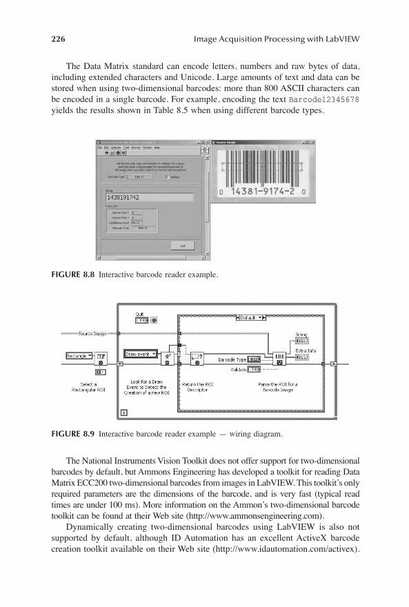
226 Image Acquisition Processing with LabVIEW
The Data Matrix standard can encode letters, numbers and raw bytes of data,including extended characters and Unicode. Large amounts of text and data can bestored when using two-dimensional barcodes: more than 800 ASCII characters canbe encoded in a single barcode. For example, encoding the text Barcode12345678yields the results shown in Table 8.5 when using different barcode types.
The National Instruments Vision Toolkit does not offer support for two-dimensionalbarcodes by default, but Ammons Engineering has developed a toolkit for reading DataMatrix ECC200 two-dimensional barcodes from images in LabVIEW. This toolkit�s onlyrequired parameters are the dimensions of the barcode, and is very fast (typical readtimes are under 100 ms). More information on the Ammon�s two-dimensional barcodetoolkit can be found at their Web site (http://www.ammonsengineering.com).
Dynamically creating two-dimensional barcodes using LabVIEW is also notsupported by default, although ID Automation has an excellent ActiveX barcodecreation toolkit available on their Web site (http://www.idautomation.com/activex).
FIGURE 8.8 Interactive barcode reader example.
FIGURE 8.9 Interactive barcode reader example � wiring diagram.
1480_book.fm Page 226 Tuesday, June 24, 2003 11:35 AM

Machine Vision 227
8.2.3 INSTRUMENT CLUSTERS
Soliton Automation has developed a Vision Toolkit-based inspection system thatinspects automotive instrument clusters for color, illumination and defects. The PC-based machine vision system uses National Instruments� image acquisition hardwareto capture images, and customized application software inspects the quality ofillumination, colors, sequences and currents. More information about this solution
TABLE 8.4“IMAQ Read Barcode–Extra Info” Cluster Elements
Cluster Element DescriptionSpecial character 1 Particular barcode types contain special leading
and trailing characters, as deÞned below (if special characters do not exist, these values are returned as 0):
� Codabar: start character� Code 128: function character (FNC)� EAN 8: Þrst country code� EAN 13: Þrst country code
Special character 2 This variable is similar to special character 1:� Codabar: stop character� EAN 8: second country code� EAN 13: second country code� UPCA: system number
ConÞdence level When IMAQ Read Barcode executes, it measures the relative widths of the dark and light bars in the barcode, and the conÞdence level reßects the level of error in these width measurements. ConÞdence level returns values between 0 (poor conÞdence) and 1000 (high conÞdence); generally conÞdence levels over 700 are acceptable.
FIGURE 8.10 An example of a two-dimensional barcode.
1480_book.fm Page 227 Tuesday, June 24, 2003 11:35 AM

228 Image Acquisition Processing with LabVIEW
and methods of including similar code into your own application can be found atSoliton Automation�s Web site (http://www.solitonautomation.com).
Barcode Barcode Type
Code 39 (3 of 9)
Code 128
(c)
Data Matrix
FIGURE 8.11
1480_book.fm Page 228 Tuesday, June 24, 2003 11:35 AM

229
Glossary
1-Bit Image
An image comprising pixels that contain only a single bit of infor-mation � each pixel is either on or off. Usually, �on� refers to white,while �off� is black.
4-Bit Image
An image Þle format that allows for 4 bits of image-based data perpixel. Such an image can contain up to 16 different colors or levels of gray.
8-Bit Image
An image where each pixel contains 8 bits of information. An 8-bit pixel can take on one of 256 possible values. There are two commontypes of 8-bit images: grayscale and indexed color. In grayscale images,each pixel is represented as one of 256 shades linearly distributed of grayfrom 0 (usually black) to 256 (usually white), and therefore does notrequire a palette (but often contains one anyway). Indexed color imagesalways contain a palette, and each pixel is an index to a color in the paletteof 256 colors.
24-Bit Image
A 24-bit image contains pixels made up of RGB byte triplets.
Additive Primary Colors
Red, green and blue; the colors used to create all othercolors when direct or transmitted light is used. They are called �additiveprimaries� because they produce white when superimposed.
Antialiasing
A method of Þlling data that has been missed due to undersampling.Antialiasing is often used to remove jaggies by interpolating valuesbetween pixels, reducing the stairstepping artifact often found in high-contrast digital images.
AOI
Area of interest; a rectangle within an image deÞned as two points withinthe image, with each side parallel with one of the image�s axes. See also
ROI.
Aspect Ratio
The proportion of an image�s size given in terms of the horizontallength vs. the vertical height. An aspect ratio of 4:3 indicates that theimage is 4/3 times as wide as it is high.
Bezier Curve
A curve created from endpoints and two or more control pointsthat serve as positions for the shape of the curve. Originated by P. Bezier.
Binary
A type of image in which the pixel values represent either light (1) ordark (0), with no intermediate shades of color.
Bit Block Transfer
A raster operation that moves a block of bits representingsome portion of an image or scene from one location in the frame bufferto another.
Bitmap
An image that contains a value for each of its pixels. See also
VectorImage
.
Bit Plane
A theoretical two-dimensional plane containing a single bit of memoryfor each pixel in an image.
Bounding Rectangle
The smallest rectangle that Þts around a given object, oftenrotationally restricted to be parallel to both image axes.
1480_book.fm Page 229 Tuesday, June 24, 2003 11:35 AM

230
Image Acquisition Processing with LabVIEW
BMP
Microsoft bitmap image Þle format extension.
Camera
An image sensing device where an image is formed on a plane, and theenergy of the image is sensed point by point.
Cartesian Coordinates
An equally spaced grid that uniquely assigns every pointin the space as a coordinate pair (two-dimensional:
x, y
) or triplet (three-dimensional:
x, y, z
). In imaging, each point is usually referred to as a
pixel
. Most images use the top-left as their origin (0,0). See also
Coordi-nates
.
Chroma-key
An image blending function which replaces pixels of a speciÞedhue range with pixels from a secondary image. This is often referred toas the
weatherman effect,
as weather forecasters often stand in front of asolid blue or green background, which is transformed into a weather map.
CIE
Commission Internationale de l�Eclairage.
The International Commissionof Illumination. The CIE is a standards organization that provides speci-Þcations for the description of device-independent color.
CMY/CMYK
Cyan, magenta, yellow, black. Printers coat paper with coloredpigments that remove speciÞc colors from the illumination light. CMY isthe subtractive color model that corresponds to the additive RGB model.Cyan, magenta and yellow are the color complements of red, green andblue. Due to the difÞculties of manufacturing pigments that will produceblack when mixed together, a separate black ink is often used and isreferred to as
K
(The symbol
B
cannot be used, as it represents blue).
Color Model/Space
A mathematical coordinate system used to assign numericalvalues to colors. There are many ways to deÞne such spaces, includingCMY, CMYK, IHS, HSL, HSV and RGB.
Compression
An image processing method of saving disk and memory require-ments by reducing the amount of space required to save a digital image.Image data is rewritten so that it is represented by a smaller set of data.See also
Lossless
and
Lossy
Compression.
Compression Ratio
The ratio of a Þle�s uncompressed size and its compressedsize.
Convolution
An image processing operation used to spatially Þlter an image,deÞned as a kernel. The size of the kernel, the numbers within it, andoften a single normalizer value deÞne the operation that will be appliedto the image. The kernel is applied to the image by placing the kernelover the image to be convolved and moving it through the image so thatit is individually centered over every pixel in the original image. See also
Kernel
.
Crop
An image processing method of removing a region near the edge of theimage, retaining a central area.
Decompression
Returning an image from a compressed format. See also
Com-pression
.
Dilation
See
Morphology
.
Dithering
The method of using neighborhoods of display pixels to represent oneimage intensity or color. This method allows low intensity resolutiondisplay devices to simulate higher resolution images. For example, a
1480_book.fm Page 230 Tuesday, June 24, 2003 11:35 AM
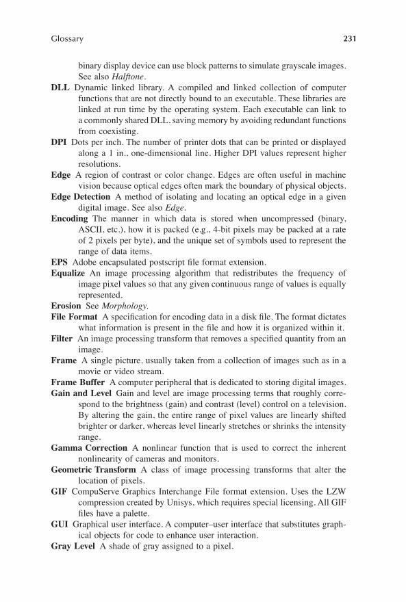
Glossary
231
binary display device can use block patterns to simulate grayscale images.See also
Halftone
.
DLL
Dynamic linked library. A compiled and linked collection of computerfunctions that are not directly bound to an executable. These libraries arelinked at run time by the operating system. Each executable can link toa commonly shared DLL, saving memory by avoiding redundant functionsfrom coexisting.
DPI
Dots per inch. The number of printer dots that can be printed or displayedalong a 1 in., one-dimensional line. Higher DPI values represent higherresolutions.
Edge
A region of contrast or color change. Edges are often useful in machinevision because optical edges often mark the boundary of physical objects.
Edge Detection
A method of isolating and locating an optical edge in a givendigital image. See also
Edge
.
Encoding
The manner in which data is stored when uncompressed (binary,ASCII, etc.), how it is packed (e.g., 4-bit pixels may be packed at a rateof 2 pixels per byte), and the unique set of symbols used to represent therange of data items.
EPS
Adobe encapsulated postscript Þle format extension.
Equalize
An image processing algorithm that redistributes the frequency ofimage pixel values so that any given continuous range of values is equallyrepresented.
Erosion
See
Morphology
.
File Format
A speciÞcation for encoding data in a disk Þle. The format dictateswhat information is present in the Þle and how it is organized within it.
Filter
An image processing transform that removes a speciÞed quantity from animage.
Frame
A single picture, usually taken from a collection of images such as in amovie or video stream.
Frame Buffer
A computer peripheral that is dedicated to storing digital images.
Gain and Level
Gain and level are image processing terms that roughly corre-spond to the brightness (gain) and contrast (level) control on a television.By altering the gain, the entire range of pixel values are linearly shiftedbrighter or darker, whereas level linearly stretches or shrinks the intensityrange.
Gamma Correction
A nonlinear function that is used to correct the inherentnonlinearity of cameras and monitors.
Geometric Transform
A class of image processing transforms that alter thelocation of pixels.
GIF
CompuServe Graphics Interchange File format extension. Uses the LZWcompression created by Unisys, which requires special licensing. All GIFÞles have a palette.
GUI
Graphical user interface. A computer�user interface that substitutes graph-ical objects for code to enhance user interaction.
Gray Level
A shade of gray assigned to a pixel.
1480_book.fm Page 231 Tuesday, June 24, 2003 11:35 AM

232
Image Acquisition Processing with LabVIEW
Grayscale
A type of image in which the pixel values are proportional to thelight intensity corresponding to a small spot in the image. Zero is usuallyblack and higher numbers indicate brighter pixels.
Halftone
The reproduction of a continuous-tone image on a device that does notdirectly support continuous output. This is done by displaying or printingpattern of small dots that from a distance can simulate the desired outputcolor or intensity.
Histogram
A tabulation of pixel value populations usually displayed as a barchart where the x axis represents all the possible pixel values and the yaxis is the total image count of each given pixel value. Each histogramintensity value or range of values is called a bin. Each bin contains apositive number that represents the number of pixels in the image thatfall within the bin�s range. When the collection of bins is charted, thegraph displays the intensity distributions of all the images pixels.
HSL
Hue, saturation and lightness. A method of describing colors as a triplet ofreal values. The hue represents the wavelength of the color, the saturationis the depth, and the lightness refers to how black or white a color is.
Huffman Encoding
A method of encoding symbols that varies the length of thecode in proportion to its information content. Groups of pixels that appearfrequently in an image are coded with fewer bits than those of loweroccurrence.
IHS
Intensity, hue and saturation.
Image Format
Refers to the speciÞcation under which an image has been savedto disk or in which it resides in computer memory. There are manycommonly used digital image formats in use, including TIFF, BMP, GIF,and JPEG. The image format speciÞcation dictates what image informa-tion is present and how it is organized in memory. Many formats supportvarious subformats.
Image Processing
The general term refers to a computer discipline whereindigital images are the main data object. This type of processing can bebroken down into several subcategories, including compression, imageenhancement, image Þltering, image distortion, image display and color-ing and image editing. See also
Machine Vision.
Intensity Graph
A native LabVIEW front panel indicator, which can display256 colors (selected, via a color table, from the available 16 million). Thevalue that is input to each pixel determines both the color and the intensitythat is displayed.
Jaggies
A term used to describe the visual appearance of lines and shapes inraster pictures that results from using a drawing grid of insufÞcient spatialresolution.
JPEG
Joint Photographic Experts Group image compression capable of bothlossy and lossless compression.
JPG
Joint Photographic Experts Group Þle format extension. See
JPEG
.
Kernel
A matrix of pixels that is used as an operator during an image convolu-tion. The kernel is set prior to the convolution in a fashion that willemphasize a particular feature of the image. Kernels are often used as
1480_book.fm Page 232 Tuesday, June 24, 2003 11:35 AM

Glossary
233
spatial Þlters, each one tuned to a speciÞc spatial frequency that theconvolution is intended to highlight. See also
Convolution
.
LZW
Lempel-Zev-Welch. An image compression method with lossless perfor-mance.
Level
See
Gain and Level
.
LUT
Look up table. A continuous block of computer memory that is initializedin such a fashion that it can be used to compute the values of a functionof one variable. The LUT is set up so that the functions variable is usedas an address or offset into the memory block. The value that resides atthis memory location becomes the functions output. Because the LUTvalues need only be initialized once, they are useful for image processingbecause of their inherent high speed. See also
Palette
.
Lossless Compression
A method of image compression where there is no lossin quality when the image is subsequently uncompressed (the uncom-pressed image is identical to its original). Lossless compression usuallyresults in a lower in compression ratio than lossy compression.
Lossy Compression
A method of image compression where some image qualityis sacriÞced in exchange for higher compression ratios. The amount ofquality degradation depends on the compression algorithm used, and itssettings.
Machine Vision
A subdiscipline of artiÞcial intelligence that uses video camerasor scanners to obtain information about a given environment. Machinevision processes extract information from digital images about objects inthe image. Machine vision takes an image in and outputs some level ofdescription about the objects in it (i.e., color, size, brightness). See also
Image Processing
.
Morphing
An imaging process where one image is gradually transformed intoa second image, where both images previously exist. The result is asequence of in-between images which when played sequentially give theappearance of the starting image being transformed to the second image.Morphing is made up of a collection of image processing algorithms. Thetwo major groups are warps and blends.
Morphology
A neighborhood image processing algorithm similar to image con-volution except that Boolean logic is applied instead of arithmetic. Thereare two types of morphology: binary and grayscale. The four major mor-phology operations are:� Erosion: a Þlter which tends to make bright objects smaller.� Dilation: a Þlter which tends to make bright objects larger.� Opening: an erosion followed by a dilation.� Closing: a dilation followed by an erosion.
Neighborhood Process
A class of image processing routines that works onneighborhoods of pixels at a time. Each pixel in the new image is com-puted as a function of the neighborhood of the pixel from the originalpixel. See also
Point Process.
MPEG
Moving Pictures Experts Group image compression.
1480_book.fm Page 233 Tuesday, June 24, 2003 11:35 AM

234
Image Acquisition Processing with LabVIEW
MUTEX
Mutual exclusion object. A program object that allows multiple pro-gram threads to share the same resource, such as Þle access, but notsimultaneously. When a program is started, a MUTEX is created with aunique name, and then any thread that needs the resource must lock theMUTEX from other threads while it is using the resource. The MUTEXis set to unlock when the data is no longer required or the routine isÞnished.
Overlay
An object, image or subimage that can be placed over a given image.The pixels from the original image are not altered, but the overlay can beviewed as if they had been. Usually used to place temporary text andannotation marks such as arrows and company logos over an image.
Packed Bits
When a binary image is usually stored in computer memory 8 pixelsper byte. Using this technique saves memory, but makes reading andwriting any individual pixel somewhat more difÞcult, as most PCs cannotdirectly access memory in chunks smaller than a byte.
Palette
A digital images palette is a collection of 3 LUTs, which are used todeÞne a given pixels display color; one LUT for red, one for green andone for blue. A palette image requires its palette in order to be displayedin a fashion that makes sense to the viewer (without a palette describingwhat color each pixel is to be displayed with, images are most likelydisplayed as randomly selected noise). A grayscale palette occurs wheneach of the 3 LUTs are linear, as since each color component (R, G, B)will be an equal value, any pixels input to them will be displayed in avarying shade of gray. See also
LUT
.
Pattern Recognition/Recognition
A subdiscipline of machine vision whereimages are searched for speciÞc patterns. Optical character recognition(OCR) is one type of pattern recognition, where images are searched forthe letters of the alphabet.
PCX
ZSoft Corporation picture Þle format extension.
Picture Indicator
A native LabVIEW front panel indicator that can display 32-bit color, using 8 bits for each color, R, G and B, with the left-most byte(
a
) unused. The intensity of each pixel in the picture control�s coloredimage is proportional (for a linear gamma curve) to the sum of the RGBvalues. The color of each pixel is determined by the ratio of the RBGvalues for that pixel.
Pixel
Picture element. The most fundamental element of a bitmap image.
Point Process
A class of image processing that mathematically transforms eachpixel individually, with no weighting from neighboring pixel intensities.
Posterize
A special effect that decreases the number of colors or grayscales inan image.
Pseudocolor
A method of assigning color to ranges of a grayscale image�s pixelvalues. Most often used to highlight subtle contrast gradients or for visu-ally quantifying pixel values. The applied color usually has no correspon-dence to the original, physical imaged scene.
Render
The process of displaying an image.
1480_book.fm Page 234 Tuesday, June 24, 2003 11:35 AM

Glossary
235
Resolution
There are two types of resolution in digital images: spatial andintensity. Spatial resolution is the number of pixels per unit of lengthalong the x and y axis, whereas intensity resolution is the number ofquantized brightness levels that a pixel can have.
RGB
Red, green, blue. A triplet of numeric values used to describe a color.
ROI
Region of interest. A speciÞcation structure that allows for the deÞnitionof arbitrarily shaped regions within a given image. A ROI is a placeholderthat remembers a location within an image. The ROI can encompass theentire image. See also
AOI.
Scan line
See Raster.
Screen Coordinates
Screen coordinates are those of the actual graphics displaycontroller, with its origin at the upper lefthand corner of the display. Seealso
Coordinates.Segment A contiguous section of a raster line deÞned in physical coordinates
by the triplet of its left-most point and length (x, y, l).Systems Integrator A service provider who can deliver a custom hardware and
software system, integrating various components from different manufac-turers, often writing custom software and fabricating custom hardware.
TGA TrueVision Corporation Þle format extension.TIFF Tagged Image File Format extension.Thumbnail A small copy of an image usually used to display many images on
the screen at once in a browser conÞguration.Transform An algorithm that alters an image, often written as xform. See also
Point Transform, Neighborhood Transform and Geometric Transform.Triplet Three numbers which when used together represent a single quantity or
location (e.g., RGB or x, y, z.)Umbras Portions of a shadow that are neither totally light nor totally dark.Video Signal A time varying signal where the amplitude of the signal is pro-
portional to the light sensed on a point in the image, and the elapsed timeidentiÞes the location of the sensed point in an image.
Video Stream A sequence of still images that are transmitted and displayed insynchronous order given the appearance of live motion.
WMF Microsoft Corporation Windows MetaFile Format Þle format extension.WPG Word Perfect Corporation Þle format extension.
1480_book.fm Page 235 Tuesday, June 24, 2003 11:35 AM

1480_book.fm Page 236 Tuesday, June 24, 2003 11:35 AM

237
Bibliography
TEXTS
IMAQ Vision Concepts Manual,
2002, National Instruments
LabVIEW Advanced Programming Techniques,
Bitter, Mohiuddin, andNawrocki, 2001, CRC Press LLC
LabVIEW Graphical Programming (2nd ed.),
Gary W. Johnson, 1997,McGraw Hill
LabVIEW Power Programming,
Gary W. Johnson, 1998, McGraw Hill
National Instruments Developer Zone,
http://zone.ni.com
National Instruments LabVIEW Zone,
http://www.ni.com/devzone/lvzone
Shape Analysis and ClassiÞcation,
Luciano da Fontoura Costa and RobertoMarcondes Cesar Jr., 2001, CRC Press LLC
The Engineering Handbook,
Richard C. Dorf, 2003, CRC Press LLC
The Image Processing Handbook (4th ed.),
John C. Russ, 2002, CRC Press
ONLINE RESOURCES
On a General Theory of Connectivity in Image Analysis, Ulisses Braga-Netoand John Goutsias, Center for Imaging Science and Department of Elec-trical and Computer Engineering, The Johns Hopkins University,http://cis.jhu.edu/~ulisses/papers/01-nsip.pdf
OpenG.org, the largest Open Source LabVIEW� development community,http://www.OpenG.org
The Info-LabVIEW Mailing List, http://www.info-labview.orgPattern Recognition in One Dimension, http://www.math-2000.comSearchVIEW.net, �The Starting Point for LabVIEW on the Net,�
http://www.searchview.netThe Find All VIs Project, David A. Moore, http://www.mooregoodideas.comWhat is Telecentricity?, Jim Michalski, Edmund Optics,
http://www.edmundoptics.com/techsupport/DisplayArticle.cfm?articleid=261
COMPLETELY IRRELEVANT RESOURCES
Calvin and Hobbes, Bill Watterson, http://www.ucomics.com/calvinandhobbesIndustrious 2001, Mono*Crafts, http://www.yugop.com/ver3/stuff/03/ßa.htmlMelvin Kaminsky�s biography, �I cut my Þnger: that�s tragedy. A man walks
into an open sewer and dies: that�s comedy!� http://us.imdb.com/M/person-biography?Mel+Brooks
1480_book.fm Page 237 Tuesday, June 24, 2003 11:35 AM

238
Image Acquisition Processing with LabVIEW
Tooheys Old Black Ale, http://www.australianbeers.com/beers/ tooheys_old/tooheys_old.htm
When in the USA, the author prefers Shiner Bock, http://www.shiner.com
1480_book.fm Page 238 Tuesday, June 24, 2003 11:35 AM
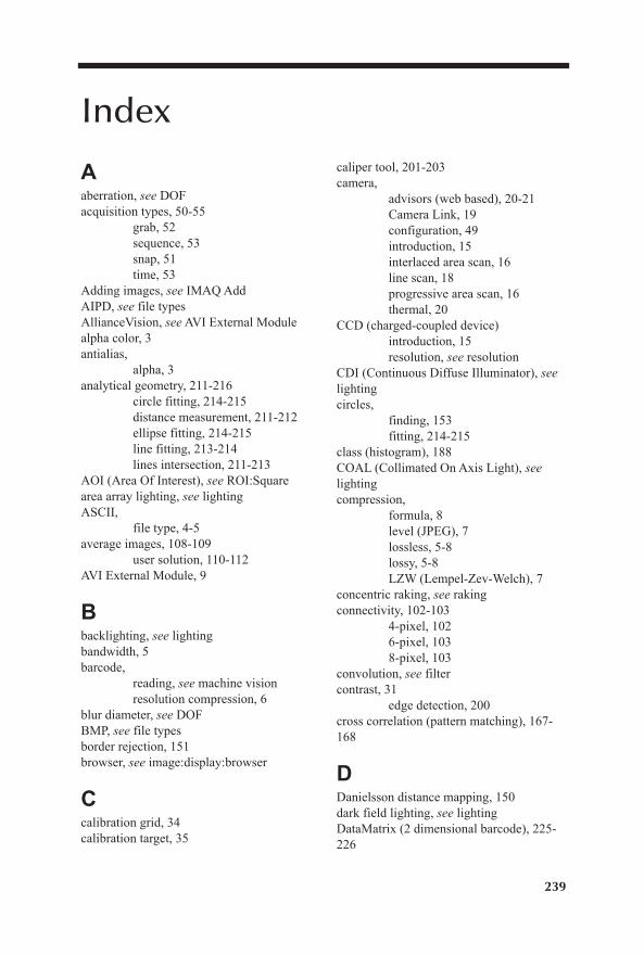
239
Index
A
aberration,
see
DOFacquisition types, 50-55
grab, 52sequence, 53snap, 51time, 53
Adding images,
see
IMAQ AddAIPD,
see
file typesAllianceVision,
see
AVI External Modulealpha color, 3antialias,
alpha, 3analytical geometry, 211-216
circle fitting, 214-215distance measurement, 211-212ellipse fitting, 214-215line fitting, 213-214lines intersection, 211-213
AOI (Area Of Interest),
see
ROI:Squarearea array lighting,
see
lightingASCII,
file type, 4-5average images, 108-109
user solution, 110-112AVI External Module, 9
B
backlighting,
see
lightingbandwidth, 5barcode,
reading,
see
machine visionresolution compression, 6
blur diameter,
see
DOFBMP,
see
file typesborder rejection, 151browser,
see
image:display:browser
C
calibration grid, 34calibration target, 35
caliper tool, 201-203camera,
advisors (web based), 20-21Camera Link, 19configuration, 49introduction, 15interlaced area scan, 16line scan, 18progressive area scan, 16thermal, 20
CCD (charged-coupled device)introduction, 15resolution,
see
resolutionCDI (Continuous Diffuse Illuminator),
see
lightingcircles,
finding, 153fitting, 214-215
class (histogram), 188COAL (Collimated On Axis Light),
see
lightingcompression,
formula, 8level (JPEG), 7lossless, 5-8lossy, 5-8LZW (Lempel-Zev-Welch), 7
concentric raking,
see
rakingconnectivity, 102-103
4-pixel, 1026-pixel, 1038-pixel, 103
convolution,
see
filtercontrast, 31
edge detection, 200cross correlation (pattern matching), 167-168
D
Danielsson distance mapping, 150dark field lighting,
see
lightingDataMatrix (2 dimensional barcode), 225-226
1480_idx.fm Page 239 Tuesday, June 24, 2003 2:08 PM

240
Image Acquisition Processing with LabVIEW
DataSocket Read,rip image from web page, 70
distance contouring, 148-151distance measurement,
see
analytical geometrydivider (kernel sum),
see
filterDOAL (Diffuse On Axis Light),
see
lightingDOF (Depth Of Field), 31dome lighting,
see
lighting
E
edge detection, 199-206edge pairs,
see
caliper toolellipse (fitting), 214-215equalization, 122-124extrapolation of lines,
see
analytical geometry
F
FFT (Fast Fourier transform),complex image types, 4
FOV (Field Of View), 30file types, 4-5
AIPD, 8BMP, 8Custom, 12GIF, 7JPEG, 7other, 8PNG, 8prototyping, 137-139TIFF, 7
fill,image portions, 181overlaid shapes, 78
filter, 130-139custom, 137directional,
see
gradientdirectionless,
see
Laplacianedge detection, 135Gaussian, 132gradient, 133Laplacian, 135linear, 130low pass, 131high pass, 131nonlinear, 130smoothing, 137
width,
see
edge detectionFireWire,
see
IEEE 1394frame overlaid shapes, 78frame grabber,
see
image:acquisition:hardwarefrequency,
complex image types, 4fitting,
see
analytical geometry
G
geometric modeling (pattern matching), 170geometery,
see
analytical geometeryGIF,
see
file typesglobal rectangle,
ROI creation, 95
H
histograph, 187-188histogram, 187-188HSL (Hue-Saturation-Luminance)
color representation, 2
I
ICO,
see
file types (other)IEEE 1394 (FireWire),
bus, 27-28cameras, 28camera configuration, 48introduction, 26NI-IMAQ for IEE 1394, 54repeater, 28
image,acquisition,
configuration, 47hardware, 25TWAIN, 59USB,
see
USBVGA signal, 59
analysis, data clusters, 10depth, 2display, 65-84browser, 74-77embed in panel, 71picture indicator, 68-70intensity graph, 67introduction, 65simple, 65-67
1480_idx.fm Page 240 Tuesday, June 24, 2003 2:08 PM

Index
241
types, 1Image Toolbox, The,
see
file types (other)
IMAQ Add, 103-105IMAQ BasicOCR, 220IMAQ BuildKernel, 137IMAQ CaliperTool, 201-203IMAQ ComplexOCR, 220IMAQ ConcentricRake, 204-205IMAQ Convolute, 131IMAQ CountObjects, 194-197IMAQ Danielsson, 150IMAQ Dispose, 66IMAQ Distance, 148IMAQ Divide, 108IMAQ EdgeTool, 199IMAQ Equalize, 123IMAQ Extract, 88IMAQ FillImage, 181IMAQ FindCircles, 153IMAQ FitCircle, 214-215IMAQ FitEllipse, 214-215IMAQ FitLine, 213-214IMAQ GetLCDROI, 223IMAQ GetPalette,
saving custom file formats, 11IMAQ GetPixelLine, 178IMAQ GetPixelRow, 178IMAQ GetRowCol, 178IMAQ Grab, 52IMAQ GrayMorphology, 144IMAQ Histograph, 187-188IMAQ Histogram, 187-188IMAQ ImageToArray,
intensity graph, 67mathematical manipulation of
images, 178IMAQ LightMeter(Line), 194IMAQ LightMeter(Point), 194IMAQ LinesIntersect,
see
analytical geometryIMAQ Modulo, 108IMAQ Morphology, 144IMAQ MulDiv, 108IMAQ Multiply, 108IMAQ OCRCorrectionConfig, 220-221IMAQ OCRRecognitionConfig, 218-219IMAQ Overlay Bitmap, 78IMAQ Overlay Text, 77
IMAQ PointDistances,
see
analytical geometryIMAQ Rake, 203-204IMAQ ReadBarcode, 225-226IMAQ Readfile,
reading image files, 9-13IMAQ ReadLCD, 223IMAQ RejectBorder, 153IMAQ ROI Profile, 86, 194, 199IMAQ Rotate, 115-116
interpolation, 116replace value, 115
IMAQ SetPixelLine, 178IMAQ SetPixelRow, 178IMAQ SetRowCol, 178IMAQ SetupLearnPattern, 171IMAQ SetupMatchPattern, 171IMAQ Sequence, 53IMAQ Snap, 51IMAQ Spoke,
see
rakingIMAQ Subtract, 105-107IMAQ Symmetry, 113-114IMAQ 3D View, 117IMAQ Threshold, 120-121IMAQ WindClose, 66IMAQ WindDraw, 66IMAQ WindLastEvent,
ROI tracing, 92use, 93
IMAQ WindSetup, 73IMAQ WindToolsMove, 81IMAQ WindToolsSetup, 81IMAQ WindToolsShow, 81IMAQ Writefile,
saving custom file formats, 11IMAQ Unwrap, 89
application, 116intensity graph,
see
image:display:intensity graphintensity profile, 195-195interlace fields, 16interlaced area scan,
see
scan typesinterlacing standards, 17-18interpolation,
bi-linear, 116zero-order, 116
interval range (histogram), 188iris,
see
DOFIVision Toolkit, 59
1480_idx.fm Page 241 Tuesday, June 24, 2003 2:08 PM
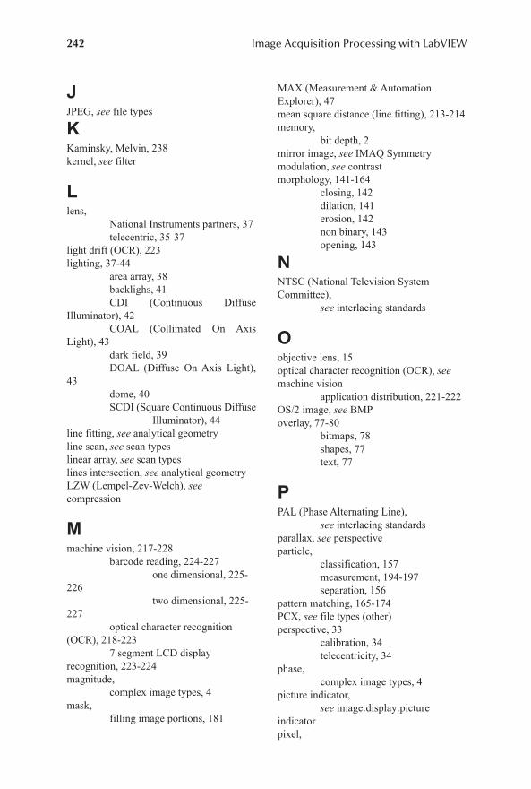
242
Image Acquisition Processing with LabVIEW
J
JPEG,
see
file types
K
Kaminsky, Melvin, 238kernel,
see
filter
L
lens,National Instruments partners, 37telecentric, 35-37
light drift (OCR), 223lighting, 37-44
area array, 38backlighs, 41CDI (Continuous Diffuse
Illuminator), 42COAL (Collimated On Axis
Light), 43dark field, 39DOAL (Diffuse On Axis Light),
43dome, 40SCDI (Square Continuous Diffuse
Illuminator), 44line fitting,
see
analytical geometryline scan,
see
scan typeslinear array,
see
scan typeslines intersection,
see
analytical geometryLZW (Lempel-Zev-Welch),
see
compression
M
machine vision, 217-228barcode reading, 224-227
one dimensional, 225-226
two dimensional, 225-227
optical character recognition (OCR), 218-223
7 segment LCD display recognition, 223-224magnitude,
complex image types, 4mask,
filling image portions, 181
MAX (Measurement & Automation Explorer), 47mean square distance (line fitting), 213-214memory,
bit depth, 2mirror image,
see
IMAQ Symmetrymodulation,
see
contrastmorphology, 141-164
closing, 142dilation, 141erosion, 142non binary, 143opening, 143
N
NTSC (National Television System Committee),
see
interlacing standards
O
objective lens, 15optical character recognition (OCR),
see
machine vision
application distribution, 221-222OS/2 image,
see
BMPoverlay, 77-80
bitmaps, 78shapes, 77text, 77
P
PAL (Phase Alternating Line),
see
interlacing standardsparallax,
see
perspectiveparticle,
classification, 157measurement, 194-197separation, 156
pattern matching, 165-174PCX,
see
file types (other)perspective, 33
calibration, 34telecentricity, 34
phase,complex image types, 4
picture indicator,
see
image:display:picture indicatorpixel,
1480_idx.fm Page 242 Tuesday, June 24, 2003 2:08 PM

Index
243
depth, 2radius (line fitting), 214
PNG,
see
files typesfile header, 8ROI information, 8
pointer,
see
image data clustersprofile,
see
intensity profileprogressive area scan,
see
scan typespolarity (edge detection), 200PXI (Portable eXtensions for Instrumentation), 26pyramidal pattern matching, 169pyroelectric,
see
camera:thermal
Q
QuickTime, 125
R
raking, 203-206concentric, 204-205parallel, 203-204spoke, 205-206
raster, 1recognition configuration (OCR), 218-219reflect image,
see
IMAQ Symmetryresolution, 30-31
calculation example, 31RGB (Red-Green-Blue)
color representation, 2ROI (Region Of Interest), 85-97
annulus arc ROI, 89descriptor, building manually, 93introduction, 85line ROI, 86oval ROI, 88rotated rectangle ROI, 89square ROI, 86tracing, 92rectangular ROI, 86
rotate image,
see
IMAQ Rotaterotational invariant pattern matching, 168-169RS-170,
see
interlacing standards
S
scale invariant pattern matching, 168-169scan types, 16
interlaced area scan, 16
line scan, 18progressive area scan, 16
SCDI (Square Continuous DiffuseIlluminator),
see
lightingSetup2Go application installation utility, 2237 segment LCD recognition,
see
machine visionskip table, 53spatial measurements (manual), 197-199spectrometer,
see
linear arrayspoke raking,
see
rakingstructuring element,
see
morphologysubtract images,
see
IMAQ Subtractsurface graph, 2surface plot, 2S-Video,
see
interlacing standards
T
tab-delimited,image file type, 5
telecentricity, 35-37template (pattern matching), 166thermoconductive,
see
camera:thermalthermoelectric,
see
camera:thermal3D data representation,
see
IMAQ 3D Viewthresholding an image, 118-122thumbnail,
see
image:display:browserTIFF,
see
file typestools palette,
see
vision window tools palettetransparency, 3TWAIN, 59type,
color, 3complex, 4grayscale, 2image, 1
U
Unwrap image,
see
IMAQ UnwrapUSB (Universal Serial Bus),
acquiring images, 56bus, 29cameras, 29introduction, 29
user solutions,
1480_idx.fm Page 243 Tuesday, June 24, 2003 2:08 PM

244
Image Acquisition Processing with LabVIEW
Automated Instrumentation for the
Assessment of Peripheral Vascular
Function, 189Combining High-Speed Imaging
and Sensors for Fast Event
Measurement, 60Connector Pin Inspection using
Vision, 175Digital Imaging and
Communications in Medicine (DICOM) for
LabVIEWDynamic Microscopy in Brain Research, 98Image Averaging with LabVIEW, 110Image Processing with Mathematica Link for LabVIEW, 183QuickTime for LabVIEW, 125Sisson-Ammons Video Analysis (SAVA) of CBFs, 207Webcam Image Acquisition, 56X-Ray Inspection System, 22
V
VFW (Video For Windows) image acquisition,
see
IVision ToolkitVGA signal, acquiring, 59Vidicon tube, 15vision window tools palette, 81-84
annulus tool, 83broken line tool, 83free tool, 83freehand line tool, 83line tool, 82oval tool, 82pan tool, 83point tool, 81polygon tool, 83rectangle tool, 82rotated rectangle tool, 83selection tool, 81zoom tool, 83
W
window,parent-child relationship, 73
WMF,
see
file types (other)
Z
Zou, George,
see
file types (other)
1480_idx.fm Page 244 Tuesday, June 24, 2003 2:08 PM


![[Penting]Data Acquisition With LabView](https://static.fdocuments.us/doc/165x107/577d20cf1a28ab4e1e93ced8/pentingdata-acquisition-with-labview.jpg)