Journal of ELECTRICAL ENGINEERING, VOL. 61, NO. 3, 2010, 149–156

IM BASED SPEED SERVODRIVEWITH LUENBERGER OBSERVER

Juraj Gacho — Milan Zalman∗

The article concerns observing states of the Induction Motor (IM) using a Luenberger observer in the speed servo drive.The movement of the motor and observer roots is analyzed for a variable speed. Following the analysis, a new method forgain evaluation of the IM magnetic flux observer is presented. This structure is extended by including an adaptive speedobserver. The functionality of the presented method is proved in simulations using MATLAB Simulink.

K e y w o r d s: induction motor, sensorless speed control, Luenberger observer

1 INTRODUCTION

Dynamic control of the IM belongs to the dominantapplications in the movement control area. In the fieldof IM control there are two noticeable two trends. Thefirst one is the control with limited measurability of thestate variables (without measuring mechanical quantities- Sensorless Control) mainly in speed drives, where themain accent is put to the quality of the state variablesobserving. The term sensorless means in this context thatsensors of mechanical quantities (position, speed, acceler-ation, torque) are not used. But if a given control struc-ture needs to have information about these quantities,they are obtained from observers. Electrical quantitieslike currents and voltages are measured in these systems.The reason for using sensorless control is that it is notnecessary to mount further sensors of mechanical quan-tities that would lead to higher costs. Furthermore themechanical sensor can be a next source of faults (mainlyin hostile environment). Using observers it is possible toreplace the older IM control types (scalar control) by su-perior control types (for example vector control) only bychanging the control algorithm.

The second trend is the closed loop dynamic controlwith focus on the speed and quality of the transient stateswith a feedback also from mechanical quantities of theIM (like position, speed). This approach is used mainlyin position systems.

In both approaches it can happen that for high-qualitycontrol also state values are needed which are not easilymeasurable in the particular structure and hence suchvalues have to be observed.

There are many methods to observe the angular speedand also further quantities needed for IM control (forexample the magnetic flux) and also many methods toobserve system parameters.

These methods can be divided into a few groups. Thereare estimators (open loop), which use the model of thesystems and also known parameters for the estimation.

Hence changes of the parameters have a strong influence

on the estimation precision. That is the reason why such

estimators are used only rarely. A few of such estimators

are mentioned in [1], [2].

Probably the largest group of the observers are based

on MRAS systems which use reference and adaptive mod-

els. Description and applications of the MRAS observers

can be found in [1], [2], [3], [4], [5], and many other works.

Applications using the extended Kalman filter (EKF)

are also often used for IM states observing. The extended

Kalman filter for observing angular speed and magnetic

flux can be found in [6], [7], [2]. The use of an extended

Luenberger observer for observing quantities of the AM

can be found in [8], [9], [10], [2]. This article concerns

the extended Luenberger observer for observing the IM

rotor magnetic flux in a speed servodrive structure with

an adaptive speed observer. In the article the calculation

is derived of the observer gains for an arbitrary position

of the observer poles and also a new method for observer

pole placement is introduced for observing the IM rotor

magnetic flux.

2 SPEED SENSORLESS DRIVE STRUCTURE

The base of the servodrive will be a squirrel cage IM.

The IM model in the stator coordinate system with state

variables is, ψr will be used. This model can be de-

scribed as

dx

dt= Ax + Bu

y = Cx

(1)

where respective matrices are

∗ Institute of Control and Industrial Informatics, Slovak University of Technology in Bratislava, Faculty of Electrical Engineering andInformation Technology, Ilkovicova 3, 812 19 Bratislava, Slovakia, juraj.gacho@amit.sk, milan.zalman@stuba.sk

ISSN 1335-3632 c© 2010 FEI STU

150 J. Gacho — M. Zalman: IM BASED SPEED SERVODRIVE WITH LUENBERGER OBSERVER

Fig. 1. Speed servodrive structure with state variable observing: SU - Starting unit (for smooth required angular speed slope, CC1, CC2- PS current controllers, MFC - PS magnetic flux controller, SC - speed controller

x =

[

isψr

]

; A =

− 1T1

(

kr

TrL′

s

− j krωL′

s

)

Lm

Tr

(

− 1Tr

+ jω)

=

[

a1 a2

a3 a4

]

B =

[

1L′

s

0

]

; C = [ 1 0 ] (2)

where

R1 = Rs +RrL2m

L2r

, T1 =L′

s

R1, Tr =

LrRr

, kr =LmLr(3)

σ = 1 −L2m

LsLr, L′

s = σLs (4,5)

In Tab.1 the symbols used in the IM model are de-scribed.

Table 1. Symbols used in the IM model

us — Stator voltageis — Stator currentΨs — Stator magnetic fluxRs — Stator resistanceLs — Stator inductanceur — Rotor voltageir — Rotor currentΨr — Rotor magnetic fluxRr — Rotor resistanceLr — Rotor inductanceLm — Magnetizing inductanceω — lectrical angular speedωs — Synchronous electrical angular speedωm — Mechanical angular speedϑ — Electrical rotor anglep′ — Number of the pole pairs

σ — Leakage factor

Used control structure for the speed servodrive withIM is presented in Fig. 1.

This article concerns mainly the IM observer block.

3 LUENBERGER OBSERVER

The Luenberger observer (LO) belongs to the group ofclosed loop observers. It is a deterministic type of observerbecause it is based on a deterministic model of the system.The basic LO is suitable only for linear time invariantsystem. This can be expressed as

dx

dt= Ax + Bu + K (y − Cx) (6)

where x is the vector of the observed state quantities andK is the observer gain matrix.

If the IM model is expressed in the stator coordinatesystem and if the elements of the stator current and rotormagnetic flux are chosen as state variables (equations (1),(2)), then we can talk about a time variant model becausethe parameters of the model can vary in time (due tochanges of the angular speed). Since the basic LO is notsuitable for the described type of system it is inevitableto use extended Luenberger observer (ELO). The ELO(unlike the basic LO) can be used also for nonlinear andtime variant systems.

The ELO design consists of two steps - appropriateselection of the observer poles and then calculation of theobserver gain matrix K .

For observing the elements of the rotor magnetic fluxvector via ELO algorithm an IM model will be used ex-pressed by equations (1).

Then the observer matrix can be written as

A0 = A − KC =

(

− 1T1

− k1

) (

kr

TrL′

s

− j krωL′

s

)

(

Lm

Tr

− k2

) (

− 1Tr

+ jω)

(7)

Journal of ELECTRICAL ENGINEERING 61, NO. 3, 2010 151

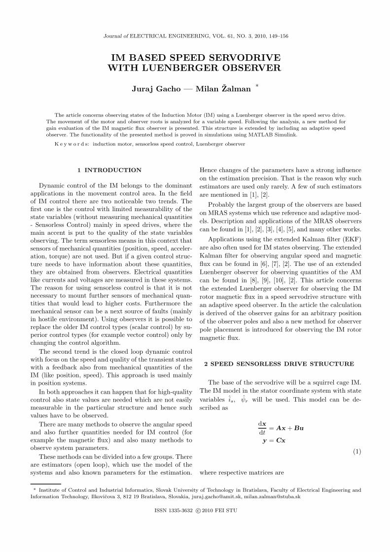
Fig. 2. Motor and observer pole placement

A special case of this type of the observer is the case when

coefficients k1 and k2 will be chosen to be zero and then

the observer matrix will be equal to the system matrix.

This approach was used in [11]. But the quality of such

an observer is not very good because there is no feedback

from the model and system outputs difference ((6), (25)).

Hence it is necessary to pay attention to the mentioned

coefficients design.

For calculation of the k1 and k2 coefficients the ob-server matrix can be written as

A0 = A − KC =

[

(a1 − k1) a2

(a3 − k2) a4

]

(8)

Observer poles placement as pLO = αejϕpIM with

constant turn angle

One of the often used possibilities how to place theobserver poles is that the poles will be (in comparisonwith the motor poles) multiplied by factor and moreoverturned by a fixed angle closer to the negative part of thereal axis. The observer poles can be then expressed as

pLO = αejϕpIM (9)

Experiments with such chosen observer poles can befound in [8].

For calculating the gain matrix coefficients k1 and k2

next equations can be used

g = |g| ejϕ = |g| (cosϕ+ j sinϕ) = gr + jgi (10)

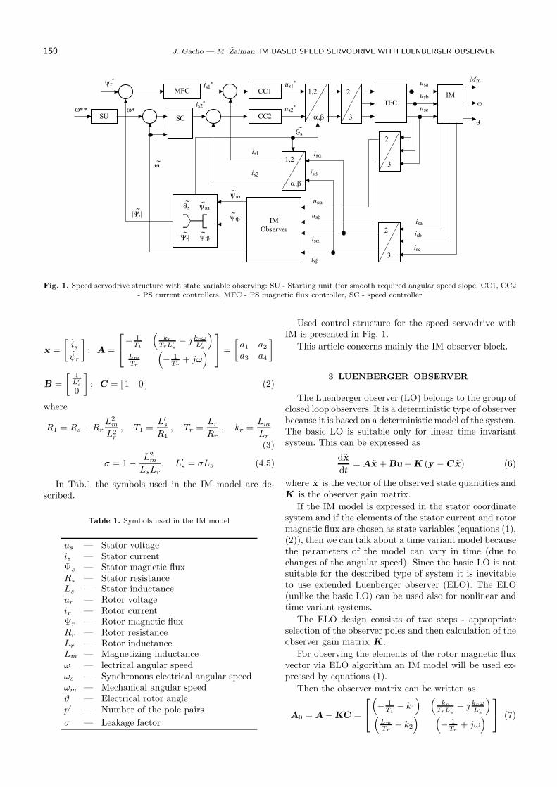
Fig. 3. Motor and observer poles for motor speed from interval-300 to 300 rad/s in continuous-time space

Fig. 4. Motor and observer poles angle for motor speed from in-terval -300 to 300 rad/s

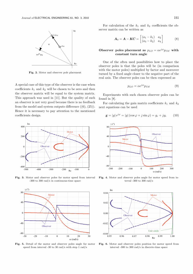
Fig. 5. Detail of the motor and observer poles angle for motorspeed from interval -30 to 30 rad/s with step 1 rad/s

Fig. 6. Motor and observer poles position for motor speed frominterval -300 to 300 rad/s in discrete-time space

152 J. Gacho — M. Zalman: IM BASED SPEED SERVODRIVE WITH LUENBERGER OBSERVER

If the original motor poles would be

pIM = |pIM | ejξ (11)

the observer poles can be written as

pLO = gpIM = |g| ejϕ |pIM | ejξ = |g| |pIM | ej(ξ+ϕ) (12)

That means it is possible to move the observer poles moreto the left side and turn them by a requested angle whichcan improve the system behavior. In this case coefficientsk1 and k2 can be written as

k1 = (g − 1)

(

1

T1+

1

Tr− jω

)

k2 = (g2 − 1)

(

L′

s

krT1−LmTr

)

−L′

s

krk1

(13)

or in components form

k11 = (gr − 1)

(

1

T1+

1

Tr

)

+ giω

k12 = (1 − gr)ω + gi

(

1

T1+

1

Tr

)

k21 =(

1 − g2r + g2

i

)

(

LmTr

−L′

s

krT1

)

−L′

s

krk11

k22 = 2grgi

(

L′

s

krT1−LmTr

)

−L′

s

krk12

(14)

It is necessary to mention that the changing sign ofthe turn angle is needed when the sign (direction) of theangular speed changes. (It will be expressed in the changeof the gi parameter sign in equations (14)).

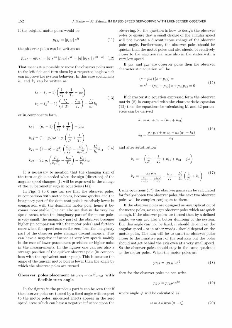
In Figs. 3 to 6 one can see that the observer poles,in comparison with motor poles, become quicker and theimaginary part of the dominant pole is relatively lower incomparison with the dominant motor pole, hence it be-comes more stable. One can also see that in the very lowspeed areas, when the imaginary part of the motor polesis very small, the imaginary part of the observer becomeshigher (in comparison with the motor poles) and further-more when the speed crosses the zero line, the imaginarypart of the observer poles changes discontinuously. Thiscan have a negative influence at very low speeds mainlyin the case of lower parameters precisions or higher noisein the measurements. In the figures one can see also astrange position of the quicker observer pole (in compar-ison with the equivalent motor pole). This is because theangle of the quicker motor pole is lower than the angle bywhich the observer poles are turned.

Observer poles placement as pLO = αejϕpIM with

flexible turn angle

In the figures in the previous part it can be seen that ifthe observer poles are turned by a fixed angle with respectto the motor poles, undesired effects appear in the zerospeed areas which can have a negative influence upon the

observing. So the question is how to design the observerpoles to ensure that a small change of the angular speedwill not evocate a discontinuous change of the observerpoles angle. Furthermore, the observer poles should bequicker than the motor poles and also should be relativelycloser to the negative real axis also in the states with avery low speed.

If po1 and po2 are observer poles then the observercharacteristic equation will be

(s− po1) (s− po2) =

= s2 − (po1 + po2) s+ po1po2 = 0(15)

If characteristic equation expressed form the observermatrix (8) is compared with the characteristic equation(15) then the equations for calculating k1 and k2 param-eters can be derived

k1 = a1 + a4 − (po1 + po2)

k2 =po1po2 + a2a3 − a4 (a1 − k1)

a2

(16)

and after substitution

k1 = −

(

1

T1+

1

Tr+ po1 + po2 − jω

)

k2 =po1po2

kr

TrL′

s

− j krωL′

s

+LmTr

−L′

s

kr

(

1

T1+ k1

)

(17)

Using equations (17) the observer gains can be calculatedfor freely-chosen two observer poles, the next two observerpoles will be complex conjugats to them.

If the observer poles are designed as -multiplication ofthe motor poles, we can get observer poles which are quickenough. If the observer poles are turned then by a definedangle, we can get also a better dumping of the system.But this angle can not be fixed, it should depend on theangular speed - or in other words - should depend on themotor poles. The aim will be to turn the observer polescloser to the negative part of the real axis but the polesshould not get behind the axis even at a very small speed.So the observer poles should stay in the same quadrantas the motor poles. When the motor poles are

pIM = |pIM | ejξ (18)

then for the observer poles ne can write

pLO = pIMαejϕ (19)

where angle ϕ will be calculated as

ϕ = λ ∗ nrm(π − ξ) (20)

Journal of ELECTRICAL ENGINEERING 61, NO. 3, 2010 153

Fig. 7. Motor and observer poles for motor speed from interval-300 to 300 rad/s in continuous-time space

Fig. 8. Motor and observer poles angle for motor speed from in-terval -300 to 300 rad/s

Fig. 9. Detail of the motor and observer poles angle for motor

speed from interval -30 to 30 rad/s with step 1 rad/s

Fig. 10. Motor and observer poles position for motor speed from

interval -300 to 300 rad/s in discrete-time space

Function nrm() recalculates the angle to be from the

range (−π , π〉 and λ is a real number from the range

〈0, 1〉 which defines how much will be the observer poles

turned to the negative part of the real axis. For λ = 0 the

observer poles will not be turned anyhow (in comparison

to the motor poles), for λ = 1 the observer poles will

be turned by an angle which ensures that the observer

poles will be on the real axis. This approach could be

described using figure Fig. 2 but the angle ϕ will depend

on the equivalent motor pole.

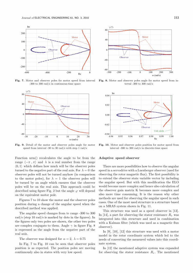
Figures 7 to 10 show the motor and the observer poles

position during a change of the angular speed when the

described method was applied.

The angular speed changes from te range -300 to 300

rad/s (step 10 rad/s is marked by dots in the figures). In

the figures only two poles are shown, the other two poles

are complex conjugats to them. Angle γ in figure Fig. 8

is expressed as the angle from the negative part of the

real axis.

The observer was designed for α = 2, λ = 0.75

In Fig. 7 to Fig. 10 can be seen that observer poles

position is as expected. The position poles are moving

continuously also in states with very low speed.

Adaptive speed observer

There are more possibilities how to observe the angularspeed in a servodrive with a Luenberger observer (used forobserving the rotor magnetic flux). The first possibility isto extend the observer state variable vector by includingthe angular speed. But with this modification the ELOwould become more complex and hence also calculation ofthe observer gain matrix K becomes more complex andalso more time consuming. It is the reason why othermethods are used for observing the angular speed in suchcases. One of the most used structure is a structure basedon a MRAS system shown in Fig. 11.

This structure was used as a speed observer in [13].In [14], a part for observing the stator resistance Rs wasintegrated into this structure and used in combinationwith a Kalman filter (which was used as a magnetic fluxobserver).

In [9], [10], [12] this structure was used with a motormodel in the rotor coordinate system which led to theneeds of converting the measured values into this coordi-nate system.

In [12] the mentioned adaptive system was expandedfor observing the stator resistance Rs . The mentioned

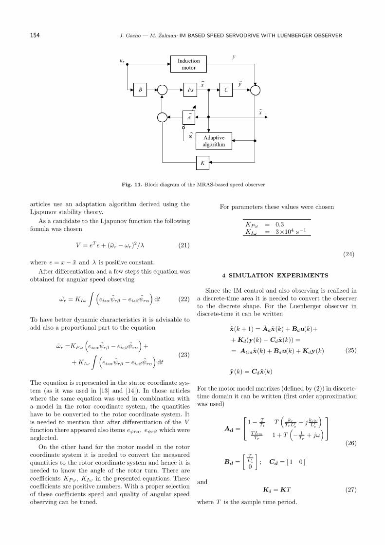
154 J. Gacho — M. Zalman: IM BASED SPEED SERVODRIVE WITH LUENBERGER OBSERVER

Fig. 11. Block diagram of the MRAS-based speed observer

articles use an adaptation algorithm derived using theLjapunov stability theory.

As a candidate to the Ljapunov function the followingfomula was chosen

V = eT e+ (ωr − ωr)2/λ (21)

where e = x− x and λ is positive constant.

After differentiation and a few steps this equation wasobtained for angular speed observing

ωr = KIω

∫

(

eisαψrβ − eisβψrα

)

dt (22)

To have better dynamic characteristics it is advisable toadd also a proportional part to the equation

ωr =KPω

(

eisαψrβ − eisβψrα

)

+

+KIω

∫

(

eisαψrβ − eisβψrα

)

dt(23)

The equation is represented in the stator coordinate sys-tem (as it was used in [13] and [14]). In those articleswhere the same equation was used in combination witha model in the rotor coordinate system, the quantitieshave to be converted to the rotor coordinate system. Itis needed to mention that after differentiation of the Vfunction there appeared also items eψrα, eψrβ which wereneglected.

On the other hand for the motor model in the rotorcoordinate system it is needed to convert the measuredquantities to the rotor coordinate system and hence it isneeded to know the angle of the rotor turn. There arecoefficients KPω, KIω in the presented equations. Thesecoefficients are positive numbers. With a proper selectionof these coefficients speed and quality of angular speedobserving can be tuned.

For parameters these values were chosen

KPω = 0.3KIω = 3×104 s−1

(24)

4 SIMULATION EXPERIMENTS

Since the IM control and also observing is realized ina discrete-time area it is needed to convert the observerto the discrete shape. For the Luenberger observer indiscrete-time it can be written

x(k + 1) = Adx(k) + Bdu(k)+

+ Kd(y(k) − Cdx(k)) =

= AOdx(k) + Bdu(k) + Kdy(k)

y(k) = Cdx(k)

(25)

For the motor model matrixes (defined by (2)) in discrete-time domain it can be written (first order approximationwas used)

Ad =

1 − TT1

T(

kr

TrL′

s

− j krωL′

s

)

TLm

Tr

1 + T(

− 1Tr

+ jω)

Bd =

[

TL′

s

0

]

; Cd = [ 1 0 ]

(26)

andKd = KT (27)

where T is the sample time period.

Journal of ELECTRICAL ENGINEERING 61, NO. 3, 2010 155

Fig. 12. Observed and real (from IM-model) magnetic flux magni-tude

Fig. 13. Detail of the observed and real (from IM-model) magneticflux magnitude

Fig. 14. Observed and real (from IM-model) speed

0.0

0.8

-0.8

-0.4

0.4

Im

-0.8 -0.4 0.0 0.4 0.8Re

Fig. 15. Rotor magnetic flux vector

IM model parameters

Pn = 1.1 kWn = 2840 min−1

p′ = 1cosϕ = 0.86η = 0.71Un = 380/220 V

In = 2.6/4.5 A

Mn = 3.7 NmJ = 0.002 kgmRs = 7.6 ΩRr = 3.7 ΩLs = 0.6015 HLr = 0.6015 HLm = 0.5796 H

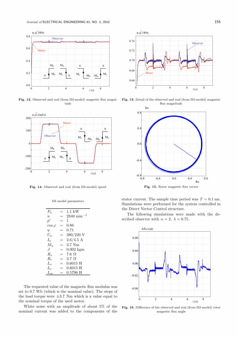
The requested value of the magnetic flux modulus wasset to 0.7 Wb (which is the nominal value). The steps ofthe load torque were ±3.7 Nm which is a value equal tothe nominal torque of the used motor.

White noise with an amplitude of about 5% of thenominal current was added to the components of the

stator current. The sample time period was T = 0.1 ms.Simulations were performed for the system controlled inthe Direct Vector Control structure.

The following simulations were made with the de-scribed observer with α = 2, λ = 0.75.

t (s)0 4 62 8

0.00

0.08

-0.08

-0.02

0.04

DJY (rad)

Fig. 16. Difference of the observed and real (from IM-model) rotor

magnetic flux angle

156 J. Gacho — M. Zalman: IM BASED SPEED SERVODRIVE WITH LUENBERGER OBSERVER

5 DISCUSSION AND CONCLUSIONS

The article concerns with the application of the ex-tended Luenberger observer for observing the rotor mag-netic flux of the induction motor. This observer was ap-plied to an IM model in a complex form. For the observerwith parameters α = 2, ϕ = 30 (modulus of the ob-server poles was twice greaterthan the modulus of themotor poles, and the observer poles were turned by 30degrees from the motor poles) the position of poles wasanalyzed during the speed change. There was seen somestrange behaviour of the observer poles in the states,when the angular speed is very low (increasing imagi-nary part of the observer poles and discontinuous changeof the observer poles, when the speed changed its direc-tion). Then a new method was proposed for designing theobserver poles position which suppressed the mentionedstrange behaviour. For simulation purposes the parame-ters of the new method were chosen as α = 2, λ = 0.75where α is a parameter (similar to the previous case)ratio of the observer and motor poles modulus and λexpresses the relative change of the observer and motorpoles phase (for the phase of the observer poles will bethe same as the phase of the motor poles, for the observerpoles will be turned by an angle which ensures that theobserver poles will be on the real axis). This method en-sures that the phases of the observer poles will be alwaysbetween the motor poles phases and the negative partof the real axis. Furthermore, the observer poles positionwill be changed continuously also when the angular speedchanges its direction.

Simulation experiments were made in a structure ofdirect vector control with the described magnetic fluxobserver and adaptive speed observer. The simulationexperiments show that the proposed observer can be usedin speed servodrives with IM also in low speed areas.

Acknowledgments

This article was elaborated as part of the grant projectVEGA 1/0690/09.

References

[1] ABELOVSK, M. : Observers of state parameters of sensorlessservo-drives with AM (Pozorovatele stavovych velicın bezsnıma-covych servopohonov s AM), Thesis, Department of Automationand Control, FEI STU, Bratislava, 2003. (in Slovak)

[2] VAS, P. : Sensorless Vector and Direct Torque Control, OxfordUniversity Press, New York, 1998.

[3] OHYAMA, K.—ASHER, G.—SUMNER, M. : Comparison ofthe Practical Performance and Operating Limits of SensorlessInduction Motor Drive using a Closed Loop Flux Observer anda Full Order Observer, EPE ’99, Lausanne 1999.

[4] ARMSTRONG, G.—ATKINSON, D. : A Comparison of ModelReference Adaptive System and Extended Kalman Filter Esti-mators for Sensorless Vector Drives, EPE ’97, Pages 1424-1429,Trondhaim 1997.

[5] SCHAUDER, C. : Adaptive Speed Identification for Vector Con-trol of Induction Motors without Rotational Transducers, IEEE

Trans. Ind. Appl. 28 No. 5, September/October (1992).

[6] BEIERKE, S.—VAS, P.—SIMOR, B.—STROANCH, A. : DSP-Controlled Sensorless AC Vector Drives Using The Extended

Kalman Filter, Intelligent Motion, 31–41, June 1997.

[7] Texas Instruments Sensorless Field Oriented Speed Control ofThree Phase AC Induction Motor using TMS320F240, TexasInstruments Europe, France, 1998.

[8] GRIVA, G.—FERRARIS, P.—PROFUMO, F.—BOJOI, R. :

Luenberger Observer for High Speed Induction Machine Drivesbased on a New Pole Placement Method, EPE 2001, Graz, 2001.

[9] MAES, J.—MELKEBEEK, J. : Adaptive Flux Observer forSensorless Induction Motor Drives with Enhanced Dynamic Per-

formance, EPE ’99, Lausanne, 1999.

[10] MAES, J.—MELKEBEEK, J. : Improved Adaptive Flux Ob-server for Wide Speed Range Sensorless Induction Motor Drives,Proc. Electromotion 6, 49-54, 1999.

[11] LEE, C., M.—CHEN, C., L. : Observer-based speed estimation

method for sensorless vector control of induction motors, IEEProc. Control Theory Appl. 145 No. 3, May 1998.

[12] MAES, J.—MELKEBEEK, J. : Speed-Sensorless Direct Torque

Control of Induction Motors Using an Adaptive Flux Obsetver,IEEE Trans. on Industry Applications v36 No. 3, 778–785May/June 1993.

[13] KUBOTA, H.—MATSUSE, K.—NAKANO, T. : DSP-Based

Speed Adaptive Flux Observer of Induction Motor, IEEE Trans.on Industry Applications 29 No. 2, 344–348 March/April 1993.

[14] MORA, J. L.—TORRALBA, A.—FRANQUELO, L. G. : ASpeed Adaptive Kalman Filter Observer For Induction Motors,

EPE 2001, Graz, 2001.

[15] GACHO, J. : Sensorless speed servo-drive with AM and obser-vation of state parameters by feedback observers (Bezsnmacovy

rychlostny servopohon s AM s pozorovanım stavovych velicınspa tnovzbovymi pozorovatel’mi), Thesis, Insitute of Control andIndustrial Informatics, FEI STU, Bratislava 2007. (in Slovak)

[16] ZALMAN, M.—ABELOVSKY, M.—JOVANKOVIC, J. : Ri-adenie v energetike, 137–142, Open speed servosystems with AM

(Otvorene rychlostne servosystemy s AM), Bratislava 2000.

Received 7 September 2009

Juraj Gacho (Ing, PhD) was born in Slovakia in 1974. Hereceived Ing. degree from the Faculty of Electrical Engineeringand Information Technology, Slovak University of Technologyin Bratislava in 1999 and PhD degree (in Automation andControl) from the same faculty in 2008. He is interested inposition control, sensorless speed control, and IM states ob-servers.

Milan Zalman (Prof PhD) was born in Slovakia in 1945.He received the MS and PhD degrees in automatic controlfrom the Slovak Technical University (STU) Bratislava in1968, 1981. He joined the Institute of Control and IndustrialInformatics, Faculty of Electrical Engineering STU where heis currently professor of automation and control. He led orparticipated in projects for industry and national researchprojects from automation of technological lines. In the lastdecade he leads national research projects in motion controlsystems with AC motors. His professional experience is in thedesign of intelligent motion control, sensorless induction mo-tor drives, fuzzy logic, neural networks and their applicationto servodrives, and implementation of DSP.