Illumination pattern optimization for fluorescence tomography: theory and simulation studies

This article has been downloaded from IOPscience. Please scroll down to see the full text article.

2010 Phys. Med. Biol. 55 2961

(http://iopscience.iop.org/0031-9155/55/10/011)

Download details:

IP Address: 128.97.129.45

The article was downloaded on 25/07/2010 at 10:14

Please note that terms and conditions apply.

View the table of contents for this issue, or go to the journal homepage for more

Home Search Collections Journals About Contact us My IOPscience

IOP PUBLISHING PHYSICS IN MEDICINE AND BIOLOGY

Phys. Med. Biol. 55 (2010) 2961–2982 doi:10.1088/0031-9155/55/10/011

Illumination pattern optimization for fluorescencetomography: theory and simulation studies

Joyita Dutta1, Sangtae Ahn1, Anand A Joshi2 and Richard M Leahy1

1 Signal and Image Processing Institute, Department of Electrical Engineering-Systems,University of Southern California, Los Angeles, CA 90089, USA2 Laboratory of Neuro Imaging, UCLA School of Medicine, Los Angeles, CA 90095, USA

E-mail: leahy@sipi.usc.edu

Received 14 October 2009, in final form 26 March 2010Published 30 April 2010Online at stacks.iop.org/PMB/55/2961

AbstractFluorescence molecular tomography is a powerful tool for 3D visualizationof molecular targets and pathways in vivo in small animals. Owing tothe high degrees of absorption and scattering of light through tissue, thefluorescence tomographic inverse problem is inherently ill-posed. In orderto improve source localization and the conditioning of the light propagationmodel, multiple sets of data are acquired by illuminating the animal surfacewith different spatial patterns of near-infrared light. However, the choice ofthese patterns in most experimental setups is ad hoc and suboptimal. This paperpresents a systematic approach for designing efficient illumination patterns forfluorescence tomography. Our objective here is to determine how to optimallyilluminate the animal surface so as to maximize the information content inthe acquired data. We achieve this by improving the conditioning of theFisher information matrix. We parameterize the spatial illumination patternsand formulate our problem as a constrained optimization problem that, for afixed number of illumination patterns, yields the optimal set of patterns. Forgeometric insight, we used our method to generate a set of three optimal patternsfor an optically homogeneous, regular geometrical shape and observed expectedsymmetries in the result. We also generated a set of six optimal patterns foran optically homogeneous cuboidal phantom set up in the transilluminationmode. Finally, we computed optimal illumination patterns for an opticallyinhomogeneous realistically shaped mouse atlas for different given numbers ofpatterns. The regularized pseudoinverse matrix, generated using the singularvalue decomposition, was employed to reconstruct the point spread functionfor each set of patterns in the presence of a sample fluorescent point sourcedeep inside the mouse atlas. We have evaluated the performance of our methodby examining the singular value spectra as well as plots of average spatial

0031-9155/10/102961+22$30.00 © 2010 Institute of Physics and Engineering in Medicine Printed in the UK 2961

2962 J Dutta et al

resolution versus estimator variance corresponding to different illuminationschemes.

(Some figures in this article are in colour only in the electronic version)

1. Introduction

Optical imaging techniques have long been popular for generating contrast representingmolecular processes in tissue. Over the past decade, their applications have extended frommicroscopy to macroscopic imaging of deep-tissue optical sources by exploiting the near-infrared (NIR) window where water, oxyhemoglobin, and deoxyhemoglobin, the primaryabsorbers in tissue, have relatively low absorption coefficients allowing light to penetrateseveral centimeters inside tissue (Weissleder and Ntziachristos 2003). The non-ionizingnature of NIR light, the availability of a variety of highly specific fluorescent probes, and,finally, low cost offer these methods some leverage over existing radiological techniques formolecular imaging (Hebden et al 1997). However, penetration depths of only a few centimetersare insufficient for most clinical deep-tissue imaging applications. Thus the success of 3Doptical imaging methods in clinical diagnostics is restricted to only a few applications. Theseinclude NIR spectroscopy and diffuse optical tomography used for mapping brain structureand function in neonates (Koizumi et al 2003, Villringer and Chance 1997, Hebden et al2002) and optical mammography for breast cancer screening (Ntziachristos and Chance 2001,Culver et al 2003). Optical tomographic methods show great promise in preclinical research,which is a valuable translational tool between in vitro studies and clinical applications.Fluorescence molecular tomography (FMT) and bioluminescence tomography (BLT) haveemerged as promising low-cost alternatives to PET and SPECT for functional imaging in smallanimals, thus greatly impacting diagnostics, drug discovery, and therapeutics (Ntziachristoset al 2005, Gibson et al 2005). Although plagued by tissue autofluorescence, FMT has manyadvantages over BLT. Compared to most bioluminescent probes, commonly used fluorophoresemit light at longer wavelengths (where tissues are less absorbing) consequently offering higherdetected signal strengths (Contag and Bachmann 2002, Hielscher 2005). Additionally multipleillumination patterns can be used to generate different mappings from the source space to thedetector space making the FMT problem less ill-posed than the BLT problem (Chaudhariet al 2005). The success of FMT can be attributed to a number of breakthroughs.

• The availability of a variety of new NIR fluorescent dyes, active or activatable fluorescentbiomarkers, and fluorescent proteins expressed by reporter genes has enabled visualizationof gene expression and several cellular and subcellular processes in vivo (Massoud andGambhir 2003, Shu et al 2009).

• Advances in instrumentation have led to the development of a range of imaging systemsfor time-domain, frequency-domain, and continuous-wave (CW) FMT (Kumar et al 2008,Godavarty et al 2005, Zavattini et al 2006). Some of the newer systems feature non-contacttomographic detection using CCD cameras with free-space detection geometries and/orinnovative optics for full-surface visualization, thus eliminating the need for optical fibersand matching fluids (Li et al 2009, Graves et al 2003, Patwardhan et al 2005).

• Finally, a number of theoretical and computational advances have led to the developmentof realistic forward models and robust inverse methods. Popular methods employed tomodel photon propagation through tissue for solving the forward problem include MonteCarlo methods (Hayakawa et al 2001, Boas et al 2002, Chen and Intes 2009) as well asanalytical and numerical solutions to the radiative transport equation (Klose et al 2002)

Illumination pattern optimization for fluorescence tomography 2963

and the diffusion equation (Rice et al 2001, Dutta et al 2008, Arridge et al 1993) subjectto different boundary conditions (Haskell et al 1994). These forward modeling schemescoupled with fast inversion techniques (Roy and Sevick-Muraca 2001, Ahn et al 2008,Zacharopoulos et al 2009) have made it feasible to reconstruct FMT images accuratelyand efficiently.

Despite their tremendous potential and increasing popularity, fluorescence tomographictechniques are confounded by high degrees of absorption and scattering of photons propagatingthrough tissue, making the FMT problem ill-posed. One approach for alleviating this problemand improving source localization is to harness spectral variations of tissue optical propertiesby using multispectral illumination and/or detection (Zacharakis et al 2005, Chaudhari et al2009). Another approach is to exploit the degree of freedom offered by external illuminationin FMT and design a set of spatial illumination patterns that improve the conditioning of theforward model matrix (Dutta et al 2009), and that is the focus of this paper.

FMT setups typically acquire data-sets corresponding to different surface illuminationpatterns. These patterns generate different excitation fields over the volume, which tune thesystem matrix. FMT setups available today employ illumination schemes chiefly guided bythe availability and simplicity of the light source. Several of these use laser sources withfocusing or diffuser lenses to generate point or distributed patch patterns (Graves et al 2003,Zavattini et al 2006, Li et al 2009). Other approaches include raster scanning (Patwardhan et al2005, Joshi et al 2006) and structured light or spatially modulated illumination patterns (Lukicet al 2009). Most of these approaches are ad hoc. Although various performance metricscould be used to theoretically compare these standard approaches, it is impossible to make anexhaustive set of comparisons, since, for a given number of illumination patterns being usedfor an experiment, infinitely many designs exist. Therefore, the question we address in thispaper is as follows: given a fixed number of illumination patterns, how do we design thesepatterns so as to maximize the information in the acquired data?

With the availability of Texas Instruments Digital Light Processor (DLP R©) chips(Hornbeck 1996, Dudley et al 2003) which work in the near-infrared range and give usprecise control over the spatial intensity distribution, it is feasible to generate any set of spatialillumination patterns with grayscale intensity variation (Gardner et al 2010, Bassi et al 2008,Konecky et al 2009, Belanger et al 2010). The focus of this paper is to compute the setof illumination patterns for CW FMT that maximize the information content in the data byimproving the conditioning of the Fisher information matrix. We formulate our problem asa constrained optimization problem that minimizes a cost function derived from the Fisherinformation matrix and computes the parameterized set of optimal spatial patterns.

Section 2 of this paper provides a description of the CW FMT problem. The formulationof the optimization problem that generates the optimal set of patterns is presented in section 3.In section 4, we describe the methods used to solve the forward and inverse problems, theoptimization procedure, and the performance metrics used to evaluate different illuminationschemes. Section 5 presents optimal patterns on a cylinder, a cuboidal tissue phantom, anda mouse atlas along with performance comparisons of illumination schemes for the atlas.Finally, a discussion of the results is presented in section 6.

2. Background

2.1. The forward problem

In continuous wave fluorescence molecular tomography (CW FMT), the 3D biodistribution ofthe fluorophore inside an animal volume is computed from the steady-state surface fluorescence

2964 J Dutta et al

photon density measured using a CCD camera. With the diffusion approximation, the CWFMT problem can be described by a set of coupled partial differential equations (PDEs)(Hutchinson et al 1995, Milstein et al 2004, Pogue and Patterson 2006):

[∇ · (−κ(r, λex)∇) + μa(r, λex)]�(r, λex) = w(r, λex), (1)

[∇ · (−κ(r, λem)∇) + μa(r, λem)]�(r, λem) = η(λem)q(r)�(r, λex). (2)

Here κ(r, λ) = 1/[3(μa(r, λ) + μ′s(r, λ))] is the diffusion coefficient and μa(r, λ) and

μ′s(r, λ), respectively, are the absorption and reduced scattering coefficients at a position r

and a wavelength λ. For a surface illumination pattern w(r, λex) at an excitation wavelengthλex, the corresponding excitation field, �(r, λex), over an animal volume, �, can be computedby solving (1). For a known fluorophore distribution q(r) and emission spectral coefficientη(λem), the emission field, �(r, λem), can be computed by solving (2) for the previouslycomputed excitation field. In FMT, we assume prior knowledge of the animal surfacegeometry and tissue optical properties, μa(r, λ) and μ′

s(r, λ). The diffusion approximationis valid under the condition μ′

s � μa . This assumption is valid for most tissue types atnear-infrared wavelengths, except near boundaries and in non-scattering parts of some organs(e.g. ventricles in the brain and alveolar sacs in the lungs) (Dehghani et al 1999). Appropriateboundary conditions must be imposed while solving (1) and (2) (Haskell et al 1994, Aronson1995). The Robin boundary condition, for example, requires that the total inwardly directedphoton current at the boundary be zero:

�(r, λex) + 2Gν · ∇(κ(r, λex)�(r, λex)) = 0, (3)

�(r, λem) + 2Gν · ∇(κ(r, λem)�(r, λem)) = 0. (4)

Here ν denotes the outward unit normal at position r on the boundary, ∂�, while G dependson the refractive index mismatch at the boundary (Schweiger et al 1995).

The PDEs (1) and (2) can be decoupled and solved subject to conditions (3) and (4),respectively, by replacing the source terms on the right-hand sides of (1) and (2) by pointsources (delta functions) at different locations. In a discretized domain with nd detector nodeson the animal surface and ns point source locations distributed inside the volume, the excitationforward model at an excitation wavelength λex can be expressed as a matrix Aex ∈ R

ns×nd ,with the j th column of this matrix representing the excitation field caused by illuminating thej th surface node. Similarly the emission forward model at an emission wavelength λem canbe expressed as a matrix Aem ∈ R

nd×ns . The j th column of this matrix represents the surfacefluorescence pattern due to the j th internal point source. For a set of p illumination patterns,we discretize the intensity distribution at the surface, w(r, λex), as a set of vectors wk ∈ R

nd ,where k = 1 : p. The solution to the forward problem is a system matrix dependent on Aex,Aem, and all the wk vectors.

The block of the system matrix corresponding to the kth illumination pattern can beobtained by diagonally scaling the emission forward model matrix by the excitation intensitiesat each internal point:

Ak = AemDexk . (5)

Here Dexk ∈ R

ns×ns is a diagonal matrix representing the excitation field due to wk and isgiven by

Dexk = diagi

(di

k

), (6)

where dik is the ith component of the vector dk computed from

Illumination pattern optimization for fluorescence tomography 2965

dk = Aexwk. (7)

The full system matrix, A ∈ Rpnd×ns , is obtained by vertically concatenating the individual

forward model matrices for a set of p different illumination patterns:

A = [A′1 A′

2 · · · A′p]′. (8)

Here the prime symbol (′) represents matrix transpose.

2.2. The inverse problem

The measured steady-state surface fluorescence patterns corresponding to p differentillumination patterns can be stacked up as a single data vector, b ∈ R

pnd . The unknownfluorophore distribution, q ∈ R

ns , can be computed by solving the following linear system ofequations:

Aq = b. (9)

CW FMT setups commonly employ one or more mirrors that make the entire surface of theobject (animal or phantom) visible in a single CCD camera image (Li et al 2009, Dutta et al2008, Chaudhari et al 2005). Such setups require CCD cameras with a high dynamic range.Mapping of this data from the CCD image space to the object space requires knowledge of theobject surface as well as calibration for various geometric and radiometric mapping parameters(Li et al 2009). The data vector, b, is obtained by interpolating CCD pixel-wise intensity valuesonto the surface mesh of the animal or phantom being imaged using the calibrated mappingscheme. Its size, therefore, depends on the mesh density.

We pose the image reconstruction problem as an optimization problem that seeks tominimize a regularized least-squares cost function:

q = arg minq

(1

2‖Aq − b‖2 +

α

2‖q‖2

). (10)

Here q is the reconstructed 3D fluorescent source distribution and α is the Tikhonovregularization parameter (Tikhonov and Arsenin 1977). The first term is a data-fitting term,while the second term is a regularization or a penalty term that smooths the reconstructedimage. The problem in (10) can be solved analytically using singular value decomposition(SVD) or using a variety of iterative methods, the former being the approach adopted in thispaper. Given the SVD, A = UΣV ′, of the system matrix, this problem can be solved usingthe regularized pseudoinverse method:

q = (A′A + αI)−1A′b= V (αI + Σ2)−1V ′(A′b). (11)

The system matrix, A, is typically very large in size, with many more rows (pnd) than columns(ns). It is often infeasible to store this large matrix in computer memory. To obtain the solutionin (11), it is sufficient to compute A′A and A′b as follows:

A′A =p∑

k=1

Dexk (Aem)′AemDex

k , (12)

A′b =p∑

k=1

dk ◦ ((Aem)′bk). (13)

Here ‘◦’ represents the Hadamard (entrywise) product and Dexk and dk can be computed from

(6) and (7), respectively. The matrix A′A ∈ Rns×ns is of the same size irrespective of the

2966 J Dutta et al

number of illumination patterns and/or the number of illumination/detection wavelengths. ItsSVD, A′A = V Σ2V ′, can be used in (11).

3. Formulation of the optimization problem

According to the Cramer Rao inequality, the inverse of the Fisher information sets a lowerbound on the variance of an unbiased estimator (Kay 1993). This establishes a reciprocitybetween the variance and the information content of an estimator. For a scalar estimator, theFisher information is a scalar, and the estimator variance can be minimized by maximizing thescalar Fisher information. However, when we are dealing with a vector estimator, the Fisherinformation is a matrix of elements, and there is no single scalar optimality criterion. In thefield of optimal design of experiments, a variety of different functionals of the eigenvaluesof the Fisher information matrix (FIM) are traditionally used as optimality criteria. Forexample, A-optimality minimizes the trace of the inverse of the FIM, D-optimality maximizesthe determinant of the FIM, and E-optimality maximizes the smallest eigenvalue of the FIM(Pukelsheim 1993). The approach that we present here is inspired by E-optimality. Ourgoal is to tune the FIM so that its singular value spectrum approaches that for the perfectlyconditioned case. Our method raises the entire spectrum in reference to the largest singularvalue. Then, for the same regularization parameter, a greater number of singular values (andthe corresponding singular vectors) will affect the solution in the optimal case, leading toimproved resolution characteristics.

In principle, an unlimited number of illumination patterns can be used. However, thiswould lead to lengthy data acquisition times (during which the animal needs to remainanesthetized), large data volumes, slow reconstruction, and possible redundancy in collecteddata, all of which are undesirable in practice. Therefore, we fix the number of patterns andseek to determine the optimal set for this given number.

3.1. Fisher information matrix

For an unknown vector q and an observed data vector b with probability density p(b), theFIM is given by (Kay 1993)

F = −E

[∂2

∂q2ln p(b)

]. (14)

We assume an additive white Gaussian noise model with the noise vector n ∼ N(0, σ 2

n I)

and the data vector b = Aq + n. Without loss of generality, we ignore the constant multiple,σ 2

n , in the covariance. Using (5) and (8), the Fisher information matrix for this system can beexpressed as

F = A′A =p∑

k=1

Dexk (Aem)′AemDex

k . (15)

Using (6), (7), and (15) the FIM can be expressed as a function of the set of illuminationpatterns, W = [w1w2 · · · wp], where W ∈ R

nd×p. We denote the ith row vector of Aex by(aex

i

)′and the ith column vector of Aem by aem

i . Then the ijth term of the FIM is given by

Fij =p∑

k=1

(w′

kaexi

)[(aem

i

)′aem

j

](w′

kaexj

)

=p∑

k=1

F emij · [(

aexi

)′wkw

′ka

exj

]

Illumination pattern optimization for fluorescence tomography 2967

= F emij ·

[(aex

i

)′p∑

k=1

(wkw′k)a

exj

]

= F emij · [(

aexi

)′WW ′aex

j

], (16)

where we have used the notations F emij = ((Aem)′Aem)ij = (

aemi

)′aem

j . This implies thatthe FIM can be conveniently represented as a Hadamard matrix product of two matrices, onedependent on the emission model and the other on the excitation model and the illuminationpatterns:

F = [(Aem)′Aem] ◦ [AexWW ′(Aex)′]. (17)

Introducing the notation F em = [(Aem)′Aem] and Gex = [AexWW ′(Aex)′], we can rewrite(17) as

F = F em ◦ Gex. (18)

3.2. Optimization problem formulation

For the system matrix, A = UΣV ′, to have a perfect condition number of 1, the diagonalmatrix Σ of singular values should be σI where σ is a singular value. Note that the singularvalue σ does not affect the condition number. Then the FIM for the ideal system is

F ideal = A′A = V Σ2V ′ = σ 2V V ′ = σ 2I. (19)

Thus, for perfect conditioning, F should approach F ideal. We would like to find a setof illumination patterns, W , which minimizes the relative difference of the resultant FIM,F (W ), and the ideal one, F ideal:

�(W , σ ) = ‖F (W ) − F ideal‖2F

‖F ideal‖2F

= ‖F (W ) − σ 2I‖2F

‖σ 2I‖2F

= 1

ns

∥∥∥∥ 1

σ 2F (W ) − I

∥∥∥∥2

F

= 1

ns

∥∥∥∥F

(W

σ

)− I

∥∥∥∥2

F

, (20)

where F (W ) is defined in (17) and ‖·‖F represents the Frobenius norm. The minimizer,(W , σ ), of the cost function, �(W , σ ), with the nonnegativity constraint W � 0 is notunique, since for any γ , �(γW , γ σ ) = �(W , σ ). We therefore first solve a simpleroptimization problem:

W opt = arg minW�0

‖F (W ) − I‖2F . (21)

Then we determine the scaling factor by imposing a power constraint, ‖W ‖F = β, on theillumination patterns. The final solution is given by

(W , σ ) = arg minσ,W�0,‖W ‖F =β

�(W , σ )

=(

β

‖W opt‖F

W opt,β

‖W opt‖F

). (22)

In practice, the illumination is scaled to exploit the maximum available source power and thusensure a high signal-to-noise ratio. Since the optimal solution, W , which minimizes �, is

2968 J Dutta et al

simply a scaled version of the solution W opt, we now focus on the simpler problem given in(21).

3.3. Dimensionality reduction

The formulated problem in (21) is fourth-order and non-convex with respect to the patterns W .W is of size nd ×p, which is typically large, and hence solving this problem is computationallyintensive (Dutta et al 2008). Additionally, the solutions are not necessarily spatially smooth.Smooth patterns are convenient for experimental implementation since calibration errors inmapping intensities from the light source to the object surface are likely to affect the accuracyof the forward model less. They are also desirable because an optimal set of patterns computedfor a mouse atlas can be meaningfully warped to any given mouse shape, as discussed laterin section 6. To allow smooth solutions and to enable speedier computation, we parameterizethe illumination patterns using a small number of spatially smooth basis functions. Thetransformation from the basis function domain to the spatial pattern domain is given by

wk = Lyk, W = LY . (23)

Here yk ∈ Rm is a vector of the linear coefficients of the basis functions for the kth illumination

pattern, L ∈ Rnd×m is a matrix whose columns are the basis vectors, and Y ∈ R

m×p withY = [y1 y2 · · · yp], m being the number of basis vectors used to encode each spatial pattern.Then, the FIM can be represented in terms of Y as follows:

F = ((Aem)′Aem) ◦ (AexLY Y ′L′(Aex)′). (24)

3.4. Modified optimization problem

With the inclusion of basis functions for dimensionality reduction, the modified optimizationproblem is as follows:

Y opt = arg minLY �0

‖F − I‖2F ,

W opt = LY opt.(25)

A gradient-based approach can be used to solve the optimization problem in (25). Our costfunction as a function of the argument yk , where k = 1 : p, is as follows:

� = ‖F − I‖2F =

ns∑i=1

ns∑j=1

(Fij − δij )2 =

ns∑i=1

ns∑j=1

�2ij , (26)

where δij is the Kronecker delta function and �ij is given by

�ij = F emij

(aex

i

)′L

(p∑

k=1

yky′k

)L′aex

j − δij . (27)

The gradient, ∇k�, of the cost function with respect to the kth argument vector, yk , is givenby

∇k� =ns∑

i=1

ns∑j=1

2�ij∇k(Fij − δij )

=ns∑

i=1

ns∑j=1

2�ijFemij

(∇kGexij

). (28)

Illumination pattern optimization for fluorescence tomography 2969

∇kGexij in (28) can be computed as follows:

∇kGexij = ∇k

((aex

i

)′L

(p∑

l=1

yly′l

)L′aex

j

)

= ∇k

((aex

i

)′Lyky

′kL

′aexj

)= L′(aex

j

(aex

i

)′+ aex

i

(aex

j

)′)Lyk. (29)

Substituting (29) in (28), we have

∇k� =ns∑

i=1

ns∑j=1

2�ijFemij L′(aex

j

(aex

i

)′+ aex

i

(aex

j

)′)Lyk. (30)

3.5. Extension to multispectral detection

Our formulation can be extended for application to multispectral detection. We assume that,for each illumination pattern, fluorescence data are collected over s wavelength bins. Thefluorescent dye is assumed to have an emission spectral coefficient ηl at the lth wavelengthbin. Then the block of the system matrix corresponding to the kth illumination pattern is givenby

Ak =

⎡⎢⎢⎢⎣

η1Aem1 Dex

k

η2Aem2 Dex

k

...

ηsAems Dex

k

⎤⎥⎥⎥⎦ . (31)

The Fisher information matrix for this case is

F =s∑

l=1

p∑k=1

(η2

l Dexk

(Aem

l

)′Aem

l Dexk

)

=(

s∑l=1

η2l

(Aem

l

)′Aem

l

)◦ (AexWW ′(Aex)′)

= F em−ms ◦ Gex, (32)

where F em−ms = (∑sl=1 η2

l

(Aem

l

)′Aem

l

). The FIM retains the Hadamard product form with

the illumination-dependent matrix Gex unchanged. This implies that, once the multispectralemission model-dependent F em−ms matrix is precomputed, the optimization problem can besolved for the multispectral emission case without any additional computational cost.

4. Methods

The optimization problem formulated in section 3 can be solved to obtain the optimalset of patterns for a given number of patterns, p. This problem is first solved for anoptically homogeneous symmetric solid shape—a cylinder—to gather geometric intuition.Next, we solve this problem for an optically homogeneous cuboidal phantom set up in thetransillumination mode with the top face illuminated and the bottom face used for detection.Finally, we solve the same problem for an optically inhomogeneous and realistically shapedmouse atlas. We perform source localization studies using the optimal patterns on the mouseatlas and evaluate the performance of the patterns based on appropriate metrics.

2970 J Dutta et al

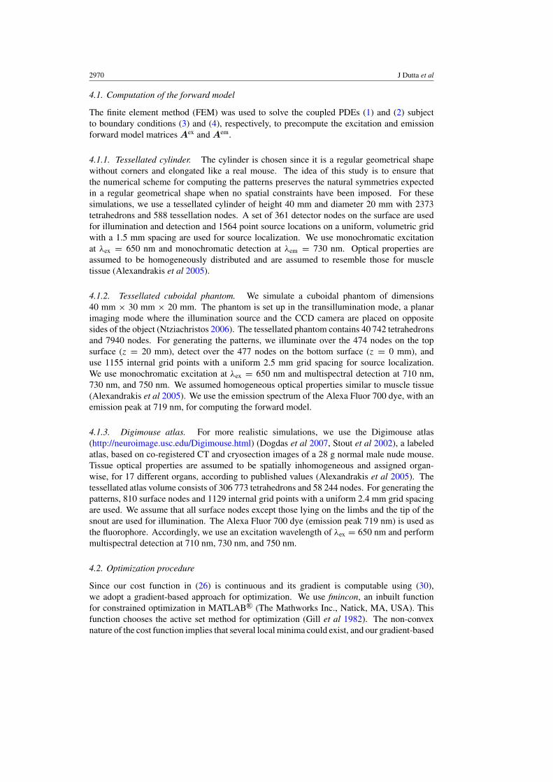
4.1. Computation of the forward model

The finite element method (FEM) was used to solve the coupled PDEs (1) and (2) subjectto boundary conditions (3) and (4), respectively, to precompute the excitation and emissionforward model matrices Aex and Aem.

4.1.1. Tessellated cylinder. The cylinder is chosen since it is a regular geometrical shapewithout corners and elongated like a real mouse. The idea of this study is to ensure thatthe numerical scheme for computing the patterns preserves the natural symmetries expectedin a regular geometrical shape when no spatial constraints have been imposed. For thesesimulations, we use a tessellated cylinder of height 40 mm and diameter 20 mm with 2373tetrahedrons and 588 tessellation nodes. A set of 361 detector nodes on the surface are usedfor illumination and detection and 1564 point source locations on a uniform, volumetric gridwith a 1.5 mm spacing are used for source localization. We use monochromatic excitationat λex = 650 nm and monochromatic detection at λem = 730 nm. Optical properties areassumed to be homogeneously distributed and are assumed to resemble those for muscletissue (Alexandrakis et al 2005).

4.1.2. Tessellated cuboidal phantom. We simulate a cuboidal phantom of dimensions40 mm × 30 mm × 20 mm. The phantom is set up in the transillumination mode, a planarimaging mode where the illumination source and the CCD camera are placed on oppositesides of the object (Ntziachristos 2006). The tessellated phantom contains 40 742 tetrahedronsand 7940 nodes. For generating the patterns, we illuminate over the 474 nodes on the topsurface (z = 20 mm), detect over the 477 nodes on the bottom surface (z = 0 mm), anduse 1155 internal grid points with a uniform 2.5 mm grid spacing for source localization.We use monochromatic excitation at λex = 650 nm and multispectral detection at 710 nm,730 nm, and 750 nm. We assumed homogeneous optical properties similar to muscle tissue(Alexandrakis et al 2005). We use the emission spectrum of the Alexa Fluor 700 dye, with anemission peak at 719 nm, for computing the forward model.

4.1.3. Digimouse atlas. For more realistic simulations, we use the Digimouse atlas(http://neuroimage.usc.edu/Digimouse.html) (Dogdas et al 2007, Stout et al 2002), a labeledatlas, based on co-registered CT and cryosection images of a 28 g normal male nude mouse.Tissue optical properties are assumed to be spatially inhomogeneous and assigned organ-wise, for 17 different organs, according to published values (Alexandrakis et al 2005). Thetessellated atlas volume consists of 306 773 tetrahedrons and 58 244 nodes. For generating thepatterns, 810 surface nodes and 1129 internal grid points with a uniform 2.4 mm grid spacingare used. We assume that all surface nodes except those lying on the limbs and the tip of thesnout are used for illumination. The Alexa Fluor 700 dye (emission peak 719 nm) is used asthe fluorophore. Accordingly, we use an excitation wavelength of λex = 650 nm and performmultispectral detection at 710 nm, 730 nm, and 750 nm.

4.2. Optimization procedure

Since our cost function in (26) is continuous and its gradient is computable using (30),we adopt a gradient-based approach for optimization. We use fmincon, an inbuilt functionfor constrained optimization in MATLAB R© (The Mathworks Inc., Natick, MA, USA). Thisfunction chooses the active set method for optimization (Gill et al 1982). The non-convexnature of the cost function implies that several local minima could exist, and our gradient-based

Illumination pattern optimization for fluorescence tomography 2971

(a) (b) (c)

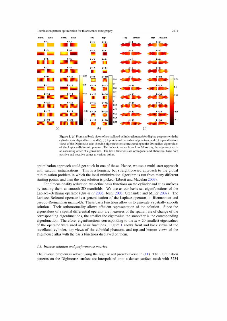
Figure 1. (a) Front and back views of a tessellated cylinder (flattened for display purposes with thecylinder axis aligned horizontally), (b) top views of the cuboidal phantom, and (c) top and bottomviews of the Digimouse atlas showing eigenfunctions corresponding to the 20 smallest eigenvaluesof the Laplace–Beltrami operator. The index k varies from 1 to 20 sorting the eigenvectors inan ascending order of eigenvalues. The basis functions are orthogonal and, therefore, have bothpositive and negative values at various points.

optimization approach could get stuck in one of these. Hence, we use a multi-start approachwith random initializations. This is a heuristic but straightforward approach to the globalminimization problem in which the local minimization algorithm is run from many differentstarting points, and then the best solution is picked (Liberti and Maculan 2009).

For dimensionality reduction, we define basis functions on the cylinder and atlas surfacesby treating them as smooth 2D manifolds. We use as our basis set eigenfunctions of theLaplace–Beltrami operator (Qiu et al 2006, Joshi 2008, Grenander and Miller 2007). TheLaplace–Beltrami operator is a generalization of the Laplace operator on Riemannian andpseudo-Riemannian manifolds. These basis functions allow us to generate a spatially smoothsolution. Their orthonormality allows efficient representation of the solution. Since theeigenvalues of a spatial differential operator are measures of the spatial rate of change of thecorresponding eigenfunctions, the smaller the eigenvalue the smoother is the correspondingeigenfunction. Therefore, eigenfunctions corresponding to the m = 20 smallest eigenvaluesof the operator were used as basis functions. Figure 1 shows front and back views of thetessellated cylinder, top views of the cuboidal phantom, and top and bottom views of theDigimouse atlas with the basis functions displayed on them.

4.3. Inverse solution and performance metrics

The inverse problem is solved using the regularized pseudoinverse in (11). The illuminationpatterns on the Digimouse surface are interpolated onto a denser surface mesh with 3234

2972 J Dutta et al

nodes. For source localization studies, a uniform grid of 9192 point sources with a 1.2 mmspacing is used. Our simulation setup uses surface data from all nodes on the atlas surfaceexcept those lying on the limbs and the tip of the snout.

In order to comparatively assess different illumination schemes, we need to establishappropriate performance metrics. We use two approaches for comparing the performanceof different illumination patterns. The first approach is to examine the conditioning ofthe system matrix corresponding to a specific illumination pattern by looking at its singularvalue distribution. The second approach is to look at average resolution–variance curves toexamine the behavior of the inverse solution.

4.3.1. Condition number. The condition number of a matrix is given by the ratio of its largestto its smallest singular value. Although this is a good figure-of-merit for the robustness ofthe system, the point spread functions (and, hence, the reconstruction results for any sourcedistribution) depend on the singular values as well as the singular vectors (Chaudhari et al2005). So in addition to looking at the condition number, we analyze properties of the pointspread functions corresponding to different source locations inside the animal volume.

4.3.2. Resolution–variance analysis. The mean squared error of an estimator can bedecomposed as a sum of the squared bias and the variance. As the regularization parameteris increased, the estimator variance decreases while the estimator bias increases (resolutionworsens) and vice versa. Resolution–variance curves, which signify this inherent tradeoff, arecommonly used to assess image reconstruction quality (Qi and Leahy 1999, Meng et al 2003,Chaudhari et al 2009). These curves are obtained by sweeping the regularization parametersover a range of values, computing the variance and resolution of the point spread functions,and plotting these two quantities against each other for the different values of the regularizationparameter. A lower lying curve implies superior resolution for the same noise variance forthe estimator corresponding to an illumination scheme. Since the regularized pseudoinverseoperator in (11) is a linear operator, it can be completely characterized in terms of its pointspread functions.

When the regularized pseudoinverse method is used for reconstruction, the spatialresolution and noise variance of the estimator can be computed in a closed form, thuseliminating the need for computationally expensive Monte Carlo simulations. For a truesource distribution q, the mean value of the estimator for a regularization parameter α can beexpressed in terms of the SVD, A = UΣV ′, of the system matrix as

E[q] = V Σ2(αI + Σ2)−1V ′q. (33)

We would like to compute the spatial resolution from the point spread function, PSFj , for thej th unit point source. For this source, q = ej , where ej is a unit vector with 1 as the j thelement. Then PSFj can be computed by substituting q = ej in (33):

PSFj = V Σ2(αI + Σ2)−1V ′ej . (34)

The spatial resolution is measured as the full width at half maximum (FWHM) computed fromPSFj . Then the average spatial resolution over n different point source locations inside theobject is a function of the regularization parameter, α:

δav(α) = 1

n

n∑j=1

FWHM{PSFj }

= 1

n

n∑j=1

FWHM{V Σ2(αI + Σ2)−1V ′ej }. (35)

Illumination pattern optimization for fluorescence tomography 2973

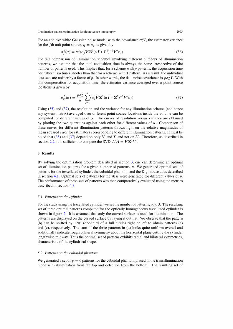
For an additive white Gaussian noise model with the covariance σ 2n I , the estimator variance

for the j th unit point source, q = ej , is given by

σ 2j (α) = σ 2

n (e′jV Σ2(αI + Σ2)−2V ′ej ). (36)

For fair comparison of illumination schemes involving different numbers of illuminationpatterns, we assume that the total acquisition time is always the same irrespective of thenumber of patterns used. This implies that, for a scheme with p patterns, the acquisition timeper pattern is p times shorter than that for a scheme with 1 pattern. As a result, the individualdata-sets are noisier by a factor of p. In other words, the data noise covariance is pσ 2

n I . Withthis compensation for acquisition time, the estimator variance averaged over n point sourcelocations is given by

σ 2av(α) = pσ 2

n

n

n∑j=1

(e′jV Σ2(αI + Σ2)−2V ′ej ). (37)

Using (35) and (37), the resolution and the variance for any illumination scheme (and henceany system matrix) averaged over different point source locations inside the volume can becomputed for different values of α. The curves of resolution versus variance are obtainedby plotting the two quantities against each other for different values of α. Comparison ofthese curves for different illumination patterns throws light on the relative magnitudes ofmean squared error for estimators corresponding to different illumination patterns. It must benoted that (35) and (37) depend on only V and Σ and not on U . Therefore, as described insection 2.2, it is sufficient to compute the SVD A′A = V Σ2V ′.

5. Results

By solving the optimization problem described in section 3, one can determine an optimalset of illumination patterns for a given number of patterns, p. We generated optimal sets ofpatterns for the tessellated cylinder, the cuboidal phantom, and the Digimouse atlas describedin section 4.1. Optimal sets of patterns for the atlas were generated for different values of p.The performance of these sets of patterns was then comparatively evaluated using the metricsdescribed in section 4.3.

5.1. Patterns on the cylinder

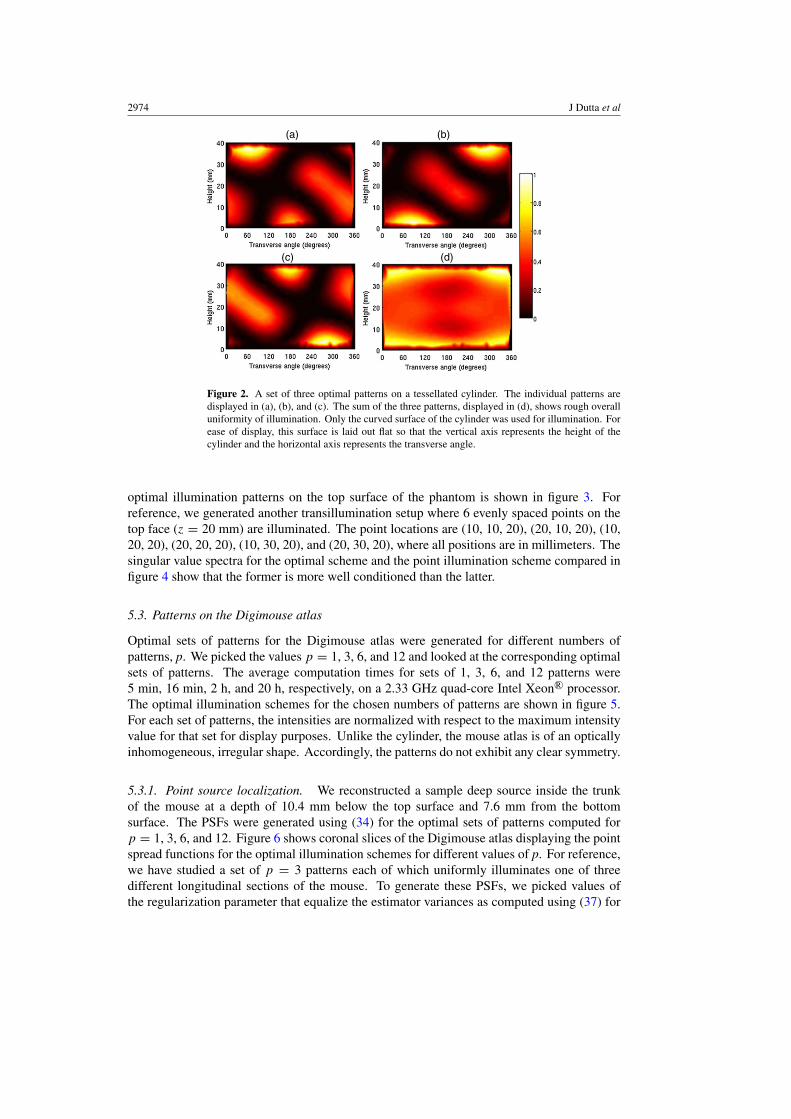
For the study using the tessellated cylinder, we set the number of patterns, p, to 3. The resultingset of three optimal patterns computed for the optically homogeneous tessellated cylinder isshown in figure 2. It is assumed that only the curved surface is used for illumination. Thepatterns are displayed on the curved surface by laying it out flat. We observe that the pattern(b) can be shifted by 120◦ (one-third of a full circle) right or left to obtain patterns (a)and (c), respectively. The sum of the three patterns in (d) looks quite uniform overall andadditionally indicate rough bilateral symmetry about the horizontal plane cutting the cylinderlengthwise midway. Thus the optimal set of patterns exhibits radial and bilateral symmetries,characteristic of the cylindrical shape.

5.2. Patterns on the cuboidal phantom

We generated a set of p = 6 patterns for the cuboidal phantom placed in the transilluminationmode with illumination from the top and detection from the bottom. The resulting set of

2974 J Dutta et al

(a) (b)

(c) (d)

Figure 2. A set of three optimal patterns on a tessellated cylinder. The individual patterns aredisplayed in (a), (b), and (c). The sum of the three patterns, displayed in (d), shows rough overalluniformity of illumination. Only the curved surface of the cylinder was used for illumination. Forease of display, this surface is laid out flat so that the vertical axis represents the height of thecylinder and the horizontal axis represents the transverse angle.

optimal illumination patterns on the top surface of the phantom is shown in figure 3. Forreference, we generated another transillumination setup where 6 evenly spaced points on thetop face (z = 20 mm) are illuminated. The point locations are (10, 10, 20), (20, 10, 20), (10,20, 20), (20, 20, 20), (10, 30, 20), and (20, 30, 20), where all positions are in millimeters. Thesingular value spectra for the optimal scheme and the point illumination scheme compared infigure 4 show that the former is more well conditioned than the latter.

5.3. Patterns on the Digimouse atlas

Optimal sets of patterns for the Digimouse atlas were generated for different numbers ofpatterns, p. We picked the values p = 1, 3, 6, and 12 and looked at the corresponding optimalsets of patterns. The average computation times for sets of 1, 3, 6, and 12 patterns were5 min, 16 min, 2 h, and 20 h, respectively, on a 2.33 GHz quad-core Intel Xeon R© processor.The optimal illumination schemes for the chosen numbers of patterns are shown in figure 5.For each set of patterns, the intensities are normalized with respect to the maximum intensityvalue for that set for display purposes. Unlike the cylinder, the mouse atlas is of an opticallyinhomogeneous, irregular shape. Accordingly, the patterns do not exhibit any clear symmetry.

5.3.1. Point source localization. We reconstructed a sample deep source inside the trunkof the mouse at a depth of 10.4 mm below the top surface and 7.6 mm from the bottomsurface. The PSFs were generated using (34) for the optimal sets of patterns computed forp = 1, 3, 6, and 12. Figure 6 shows coronal slices of the Digimouse atlas displaying the pointspread functions for the optimal illumination schemes for different values of p. For reference,we have studied a set of p = 3 patterns each of which uniformly illuminates one of threedifferent longitudinal sections of the mouse. To generate these PSFs, we picked values ofthe regularization parameter that equalize the estimator variances as computed using (37) for

Illumination pattern optimization for fluorescence tomography 2975

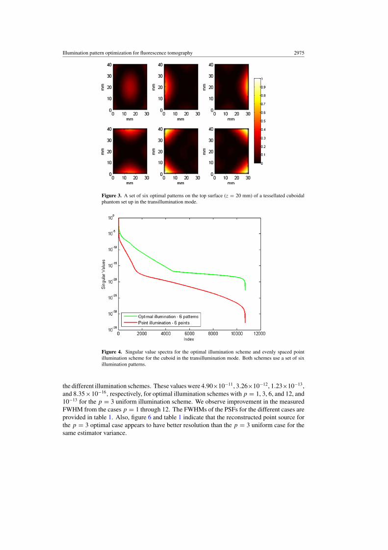
Figure 3. A set of six optimal patterns on the top surface (z = 20 mm) of a tessellated cuboidalphantom set up in the transillumination mode.

Figure 4. Singular value spectra for the optimal illumination scheme and evenly spaced pointillumination scheme for the cuboid in the transillumination mode. Both schemes use a set of sixillumination patterns.

the different illumination schemes. These values were 4.90×10−11, 3.26×10−12, 1.23×10−13,and 8.35×10−16, respectively, for optimal illumination schemes with p = 1, 3, 6, and 12, and10−13 for the p = 3 uniform illumination scheme. We observe improvement in the measuredFWHM from the cases p = 1 through 12. The FWHMs of the PSFs for the different cases areprovided in table 1. Also, figure 6 and table 1 indicate that the reconstructed point source forthe p = 3 optimal case appears to have better resolution than the p = 3 uniform case for thesame estimator variance.

2976 J Dutta et al

(d)

(a) (b)

(c)

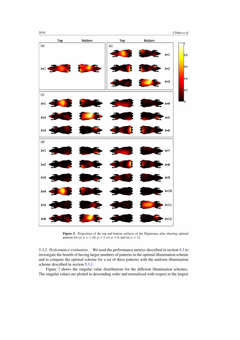
Figure 5. Projections of the top and bottom surfaces of the Digimouse atlas showing optimalpatterns for (a) p = 1, (b) p = 3, (c) p = 6, and (d) p = 12.

5.3.2. Performance evaluation. We used the performance metrics described in section 4.3 toinvestigate the benefit of having larger numbers of patterns in the optimal illumination schemeand to compare the optimal scheme for a set of three patterns with the uniform illuminationscheme described in section 5.3.1.

Figure 7 shows the singular value distributions for the different illumination schemes.The singular values are plotted in descending order and normalized with respect to the largest

Illumination pattern optimization for fluorescence tomography 2977

(a) (b) (c) (d) (e)

Figure 6. Point spread functions for (a) optimal patterns for p = 12, (b) optimal patterns forp = 6, (c) optimal patterns for p = 3, (d) uniform patterns for p = 3, and (e) optimal pattern forp = 1.

Table 1. Full width at half maximum of point spread functions in figure 6.

Pattern type FWHM (mm)

Optimal, p = 12 1.20Optimal, p = 6 1.20Optimal, p = 3 1.63Uniform, p = 3 3.02Optimal, p = 1 5.91

singular value. The condition numbers of the system matrices are provided in table 2.The condition numbers clearly improve as p is increased from 1 through 12. The optimalillumination pattern for p = 3 is observed to generate a better conditioned system matrix thanthe p = 3 uniform illumination scheme.

The plots of average resolution versus average variance for the different illuminationschemes are shown in figure 8. These are obtained by averaging resolution and variancefor n = 250 randomly picked sources on the uniform source grid for different values of theregularization parameter. The regularization parameter was swept over values within the range10−30–10−4. The best possible FWHM is 1.2 mm, which is the grid spacing. As explainedin section 4.3.2, the idea underlying these curves is the trade-off between resolution andvariance, which implies that, a decrease in estimator variance is accompanied by an increasein FWHM and vice versa. The intensities of the different sets were normalized to ensure thatall sets of patterns have the same average intensity. As expected, as p goes from 1 to 12, thecurves lie lower. In other words, the resolution–variance properties improve. Also, figure 8indicates that, for the same average variance, the p = 3 optimal illumination pattern offersbetter average resolution than the p = 3 uniform illumination scheme.

2978 J Dutta et al

Figure 7. Singular value distributions for different illumination schemes.

Figure 8. Average resolution versus variance curves for different illumination schemes.

Table 2. Condition numbers of the system matrix for different illumination schemes.

Pattern type Condition number

Optimal, p = 12 2.5575 × 109

Optimal, p = 6 1.3466 × 1010

Optimal, p = 3 7.1619 × 1011

Uniform, p = 3 2.8376 × 1012

Optimal, p = 1 3.3014 × 1013

Illumination pattern optimization for fluorescence tomography 2979

6. Discussion

We have developed an optimization framework for generating optimal spatial illuminationpatterns for CW FMT based on an approach that seeks to improve the condition number of theFisher information matrix. We formulated our problem as a constrained optimization problemwhich, for a given number of patterns, can be solved to compute the set of optimal patternswhich maximize the information content in the acquired data. Our formulation assumes ani.i.d. Gaussian noise model. The fourth-order, non-convex cost function was minimized in thepresence of a non-negativity constraint using a gradient-based approach. A multi-start methodwith random initializations was used to ensure global convergence. The dimensionality ofthe optimization problem was reduced using a set of geometrical basis functions defined onthe 2D manifold representing the surface of the object being imaged. Eigenfunctions of theLaplace–Beltrami operator were used as basis functions owing to their spatial smoothness andorthogonality. To ensure that this numerical approach is geometrically meaningful, we lookedat optimal patterns generated for an optically homogeneous tessellated cylinder and observedradial and bilateral symmetries that are intrinsic to the cylindrical shape. We then applied thismethod to compute optimal patterns for an optically homogeneous cuboidal phantom in thetransillumination mode. We compared this scheme with an evenly spaced point illuminationscheme by examining the singular value spectra and showed that the optimal scheme is morewell-conditioned than the point illumination scheme. Finally, we used our method to computeoptimal patterns for the optically inhomogeneous and realistically shaped Digimouse atlas.The obtained patterns look smooth and physically realizable. For the same number of patterns,p = 3, the optimal set was shown to perform better than a uniform illumination scheme onthe basis of condition number and average resolution versus variance curves. Since typicalFMT experimental setups use a larger number of illumination patterns, we have generatedoptimal patterns for up to p = 12 and presented their singular value spectra and averageresolution–variance characteristics. For fair comparison, the variance was computed based onthe assumption of equality of total data acquisition times for different values of p.

In our simulations, we have assumed that the entire surface of the mouse except for thelimbs and the tip of the snout is being illuminated. However, in an experimental setting, itmay not be feasible to illuminate the entire mouse surface at one go. For such applications,our formulation can be easily modified to introduce spatial constraints on the illuminationpatterns. Another useful modification of our formulation would be its extension to includemultispectral excitation. Owing to the larger variability of tissue optical properties at theexcitation wavelengths of commonly used fluorescent dyes and proteins, for the same numberof wavelength bins, multispectral excitation typically leads to a better conditioned systemmatrix than multispectral detection (Chaudhari et al 2009). We, therefore, believe that optimalillumination coupled with multispectral excitation will allow us to pack more informationinto the acquired data for a given number of illumination patterns and a given number ofwavelengths.

Currently, the main limitation of our method is the large computation time requiredto generate large numbers of patterns. We, therefore, would like to explore more efficientnumerical implementations that will enable us to compute larger sets of patterns. This willalso allow us to investigate the benefits of using large (say > 20) sets of patterns and, in theprocess, determine the minimum number of patterns that can be used without making theacquired data overly redundant.

The framework for generating optimal patterns assumes prior knowledge of mouse surfacetopography and tissue optical properties and requires the forward problem to be solved priorto the optimization procedure. It might not be feasible to repeat the optimization procedure

2980 J Dutta et al

for each animal in between the surface profiling and fluorescence data acquisition steps of anexperiment. An alternative approach would be to use the atlas as a surrogate and to warp itssurface to match that of the target mouse being imaged (Joshi et al 2009), and, in doing so,we can warp the optimal patterns onto the surface of the target.

Acknowledgments

This work was supported by the National Cancer Institute under grants R01CA121783 andR44CA138243.

References

Ahn S, Chaudhari A J, Darvas F, Bouman C A and Leahy R M 2008 Fast iterative image reconstruction methods forfully 3D multispectral bioluminescence tomography Phys. Med. Biol. 53 3921–42

Alexandrakis G, Rannou F R and Chatziioannou A F 2005 Tomographic bioluminescence imaging by use of acombined optical-pet (OPET) system: a computer simulation feasibility study Phys. Med. Biol. 50 4225–41

Aronson R 1995 Boundary conditions for diffusion of light J. Opt. Soc. Am. A 12 2532–9Arridge S R, Schweiger M, Hiroaka M and Delpy D T 1993 A finite element approach for modeling photon transport

in tissue Med. Phys. 20 299–309Bassi A, D’Andrea C, Valentini G, Cubeddu R and Arridge S 2008 Temporal propagation of spatial information in

turbid media Opt. Lett. 33 2836–8Belanger S, Abran M, Intes X, Casanova C and Lesage F 2010 Real-time diffuse optical tomography based on

structured illumination J. Biomed. Opt. 15 016006Boas D, Culver J, Stott J and Dunn A 2002 Three dimensional Monte Carlo code for photon migration through

complex heterogeneous media including the adult human head Opt. Express 10 159–70Chaudhari A J, Ahn S, Levenson R, Badawi R D, Cherry S R and Leahy R M 2009 Excitation spectroscopy in

multispectral optical fluorescence tomography: methodology, feasibility and computer simulation studies Phys.Med. Biol. 54 4687–704

Chaudhari A J, Darvas F, Bading J R, Moats R A, Conti P S, Smith D J, Cherry S R and Leahy R M 2005 Hyperspectraland multispectral bioluminescence optical tomography for small animal imaging Phys. Med. Biol. 50 5421–41

Chen J and Intes X 2009 Time-gated perturbation Monte Carlo for whole body functional imaging in small animalsOpt. Express 17 19566–79

Contag C H and Bachmann M H 2002 Advances in in vivo bioluminescence imaging of gene expression Annu. Rev.Biomed. Eng. 4 235–60

Culver J P, Choe R, Holboke M J, Zubkov L, Durduran T, Slemp A, Ntziachristos V, Chance B and Yodh A G2003 Three-dimensional diffuse optical tomography in the parallel plane transmission geometry: evaluation ofa hybrid frequency domain/continuous wave clinical system for breast imaging Med. Phys. 30 235–47

Dehghani H, Delpy D T and Arridge S R 1999 Photon migration in non-scattering tissue and the effects on imagereconstruction Phys. Med. Biol. 44 2897

Dogdas B, Stout D, Chatziioannou A and Leahy R M 2007 Digimouse: a 3D whole body mouse atlas from CT andcryosection data Phys. Med. Biol. 52 577–87

Dudley D, Duncan W M and Slaughter J 2003 Emerging digital micromirror device (DMD) applications Proc.SPIE 4985 14–25

Dutta J, Ahn S, Joshi A A and Leahy R M 2009 Optimal illumination patterns for fluorescence tomography IEEE Int.Symp. on Biomedical Imaging: From Nano to Macro, 2009 (ISBI ’09) pp 1275–8

Dutta J, Ahn S and Leahy R M 2008 Optimized illumination patterns for fluorescence tomography World MolecularImaging Conf., 2008 (WMIC’08) Abstract Book (Nice, France)

Dutta J, Ahn S, Li C, Chaudhari A J, Cherry S R and Leahy R M 2008 Computationally efficient perturbative forwardmodeling for 3D multispectral bioluminescence and fluorescence tomography Proc. SPIE 6913 69130

Gardner C, Dutta J, Mitchell G, Ahn S, Li C, Harvey P, Gershman R, Sheedy S, Mansfield J, Cherry S R, Leahy R Mand Levenson R 2010 Improved in vivo fluorescence tomography and quantitation in small animals using anovel multiview, multispectral imaging system Proc. Biomed. Optics (BIOMED) Topical Meeting (OSA) BTuF1

Gibson A P, Hebden J C and Arridge S R 2005 Recent advances in diffuse optical imaging Phys. Med. Biol.50 R1–43

Gill P E, Murray W and Wright M H (ed) 1982 Practical Optimization (New York: Academic)

Illumination pattern optimization for fluorescence tomography 2981

Godavarty A, Sevick-Muraca E M and Eppstein M J 2005 Three-dimensional fluorescence lifetime tomography Med.Phys. 32 992–1000

Graves E E, Ripoll J, Weissleder R and Ntziachristos V 2003 A submillimeter resolution fluorescence molecularimaging system for small animal imaging Med. Phys. 30 901–11

Grenander U and Miller M 2007 Pattern Theory: From Representation to Inference (New York: Oxford UniversityPress)

Haskell R C, Svaasand L O, Tsay T T, Feng T C, McAdams M S and Tromberg B J 1994 Boundary conditions forthe diffusion equation in radiative transfer J. Opt. Soc. Am. A 11 2727–40

Hayakawa C K, Spanier J, Bevilacqua F, Dunn A K, You J S, Tromberg B J and Venugopalan V 2001 PerturbationMonte Carlo methods to solve inverse photon migration problems in heterogeneous tissues Opt. Lett. 26 1335–7

Hebden J C, Arridge S R and Delpy D T 1997 Optical imaging in medicine: I. Experimental techniques Phys. Med.Biol. 42 825–40

Hebden J C, Gibson A, Yusof R M, Everdell N, Hillman E M C, Delpy D T, Arridge S R, Austin T, Meek J H andWyatt J S 2002 Three-dimensional optical tomography of the premature infant brain Phys. Med.Biol. 47 4155–66

Hielscher A H 2005 Optical tomographic imaging of small animals Curr. Opin. Biotechnol. 16 79–88Hornbeck L J 1996 Digital light processing and mems: reflecting the digital display needs of the networked society

Proc. SPIE 2783 2–13Hutchinson C, Lakowicz J and Sevick-Muraca E 1995 Fluorescence lifetime-based sensing in tissues: a computational

study Biophys. J. 68 1574–82Joshi A A 2008 Geometric methods for image registration and analysis PhD Thesis University of Southern California,

Los AngelesJoshi A A, Chaudhari A, Li C, Shattuck D, Dutta J, Leahy R M and Toga A W 2009 Posture matching and elastic

registration of a mouse atlas to surface topography range data IEEE Int. Symp. on Biomedical Imaging: FromNano to Macro, 2009 (ISBI ’09) pp 366–9

Joshi A, Bangerth W and Sevick-Muraca E M 2006 Non-contact fluorescence optical tomography with scanningpatterned illumination Opt. Express 14 6516–34

Kay S M 1993 Fundamentals of Statistical Signal Processing: Estimation Theory (Englewood Cliffs, NJ: PrenticeHall)

Klose A D, Netz U, Beuthan J and Hielscher A H 2002 Optical tomography using the time-independent equation ofradiative transfer: Part 1. Forward model J. Quant. Spectrosc. Radiat. Transfer 72 691–713

Koizumi H, Yamamoto T, Maki A, Yamashita Y, Sato H, Kawaguchi H and Ichikawa N 2003 Optical topography:practical problems and new applications Appl. Opt. 42 3054–62

Konecky S D, Mazhar A, Cuccia D, Durkin A J, Schotland J C and Tromberg B J 2009 Quantitative optical tomographyof sub-surface heterogeneities using spatially modulated structured light Opt. Express 17 14780–90

Kumar A, Raymond S, Dunn A, Bacskai B and Boas D 2008 A time domain fluorescence tomography system forsmall animal imaging IEEE Trans. Med. Imaging 27 1152–63

Li C, Mitchell G S, Dutta J, Ahn S, Leahy R M and Cherry S R 2009 A three-dimensional multispectralfluorescence optical tomography imaging system for small animals based on a conical mirror design Opt.Express 17 7571–85

Liberti L and Maculan N (ed) 2009 Global Optimization: From Theory to Implementation (New York: Springer)Lukic V, Markel V A and Schotland J C 2009 Optical tomography with structured illumination Opt. Lett. 34 983–5Massoud T F and Gambhir S S 2003 Molecular imaging in living subjects: seeing fundamental biological processes

in a new light Genes Dev. 17 545–80Meng L, Rogers W, Clinthorne N and Fessler J 2003 Feasibility study of compton scattering enchanced multiple

pinhole imager for nuclear medicine IEEE Trans. Nucl. Sci. 50 1609–17Milstein A B, Stott J J, Oh S, Boas D A, Millane R P, Bouman C A and Webb K J 2004 Fluorescence optical diffusion

tomography using multiple-frequency data J. Opt. Soc. Am. A 21 1035–49Ntziachristos V 2006 Fluorescence molecular imaging Annu. Rev. Biomed. Eng. 8 1–33Ntziachristos V and Chance B 2001 Probing physiology and molecular function using optical imaging: applications

to breast cancer Breast Cancer Res. 3 41–6Ntziachristos V, Ripoll J, Wang L and Weissleder R 2005 Looking and listening to light: the evolution of whole-body

photonic imaging Nat. Biotechnol. 23 313–20Patwardhan S, Bloch S, Achilefu S and Culver J 2005 Time-dependent whole-body fluorescence tomography of probe

bio-distributions in mice Opt. Express 13 2564–77Pogue B W and Patterson M S 2006 Review of tissue simulating phantoms for optical spectroscopy, imaging and

dosimetry J. Biomed. Opt. 11 041102

2982 J Dutta et al

Pukelsheim F 1993 Optimal Design of Experiments (Wiley Series in Probability and Mathematical Statistics) (NewYork: Wiley)

Qi J and Leahy R 1999 A theoretical study of the contrast recovery and variance of map reconstructions from pet dataIEEE Trans. Med. Imaging 18 293–305

Qiu A, Bitouk D and Miller M 2006 Smooth functional and structural maps on the neocortex via orthonormal basesof the Laplace–Beltrami operator IEEE Trans. Med. Imaging 25 1296–306

Rice B W, Cable M D and Nelson M B 2001 In vivo imaging of light-emitting probes J. Biomed. Opt. 6 432–40Roy R and Sevick-Muraca E M 2001 Three-dimensional unconstrained and constrained image-reconstruction

techniques applied to fluorescence, frequency-domain photon migration Appl. Opt. 40 2206–15Schweiger M, Arridge S R, Hiraoka M and Delpy D T 1995 The finite element method for the propagation of light

in scattering media: boundary and source conditions Med. Phys. 22 1779–92Shu X, Royant A, Lin M Z, Aguilera T A, Lev-Ram V, Steinbach P A and Tsien R Y 2009 Mammalian expression

of infrared fluorescent proteins engineered from a bacterial phytochrome Science 324 804–7Stout D, Chow P, Silverman R, Leahy R M, Lewis X, Gambhir S and Chatziioannou A 2002 Creating a whole body

digital mouse atlas with PET, CT and cryosection images Mol. Imag. Biol. 4 S27Tikhonov A N and Arsenin V Y 1977 Solutions of Ill-Posed Problems (Washington, DC: V H Winston and Sons)Villringer A and Chance B 1997 Non-invasive optical spectroscopy and imaging of human brain function Trends

Neurosci. 20 435–42Weissleder R and Ntziachristos V 2003 Shedding light onto live molecular targets Nature Med. 9 123–8Zacharakis G, Kambara H, Shih H, Ripoll J, Grimm J, Saeki Y, Weissleder R and Ntziachristos V 2005 Volumetric

tomography of fluorescent proteins through small animals in vivo Proc. Natl Acad. Sci. USA 102 18252–7Zacharopoulos A D, Svenmarker P, Axelsson J, Schweiger M, Arridge S R and Andersson-Engels S 2009 A matrix-

free algorithm for multiple wavelength fluorescence tomography Opt. Express 17 3042–51Zavattini G, Vecchi S, Mitchell G, Weisser U, Leahy R M, Pichler B J, Smith D J and Cherry S R 2006 A hyperspectral

fluorescence system for 3d in vivo optical imaging Phys. Med. Biol. 51 2029–43